Embed Size (px)
Citation preview

FIN501 Asset PricingLecture 06 Mean-Variance & CAPM (1)
LECTURE 06:MEAN-VARIANCE ANALYSIS & CAPM
Markus K. Brunnermeier

FIN501 Asset PricingLecture 06 Mean-Variance & CAPM (2)
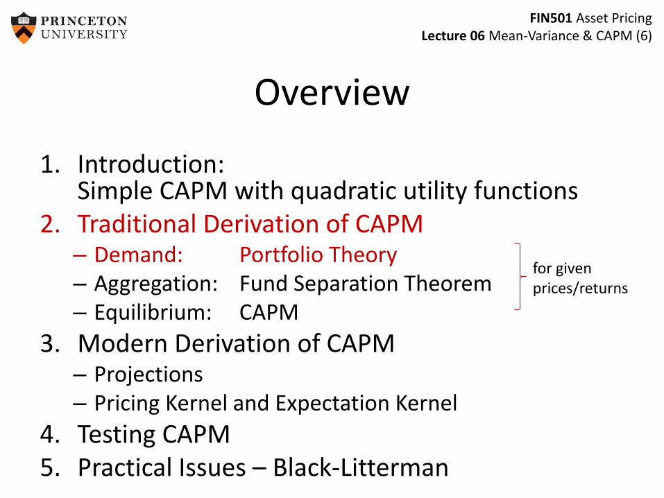
Overview
1. Introduction: Simple CAPM with quadratic utility functions(from beta-state price equation)
2. Traditional Derivation of CAPM– Demand: Portfolio Theory– Aggregation: Fund Separation Theorem– Equilibrium: CAPM
3. Modern Derivation of CAPM– Projections– Pricing Kernel and Expectation Kernel
4. Testing CAPM5. Practical Issues – Black-Litterman
for given prices/returns

FIN501 Asset PricingLecture 06 Mean-Variance & CAPM (3)
Recall State-price Beta model
Recall:
𝐸 𝑅ℎ − 𝑅𝑓 = 𝛽ℎ𝐸 𝑅∗ − 𝑅𝑓
Where 𝛽ℎ ≔cov 𝑅∗,𝑅ℎ
var 𝑅∗
very general – but what is 𝑅∗ in reality?
FIN501 Asset PricingLecture 06 Mean-Variance & CAPM (4)
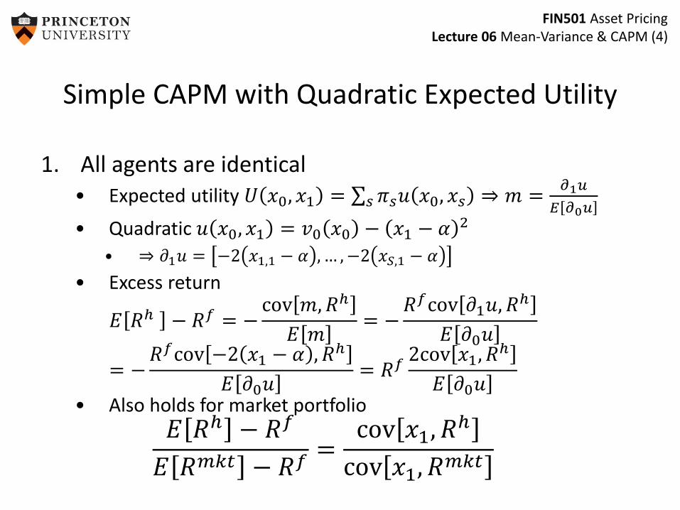
Simple CAPM with Quadratic Expected Utility
1. All agents are identical• Expected utility 𝑈 𝑥0, 𝑥1 = 𝑠 𝜋𝑠𝑢 𝑥0, 𝑥𝑠 ⇒ 𝑚 =
𝜕1𝑢
𝐸 𝜕0𝑢
• Quadratic 𝑢 𝑥0, 𝑥1 = 𝑣0 𝑥0 − 𝑥1 − 𝛼 2
• ⇒ 𝜕1𝑢 = −2 𝑥1,1 − 𝛼 , … , −2 𝑥𝑆,1 − 𝛼
• Excess return
𝐸 𝑅ℎ − 𝑅𝑓 = −cov 𝑚, 𝑅ℎ
𝐸 𝑚= −
𝑅𝑓cov 𝜕1𝑢, 𝑅ℎ
𝐸 𝜕0𝑢
= −𝑅𝑓cov −2 𝑥1 − 𝛼 , 𝑅ℎ
𝐸 𝜕0𝑢= 𝑅𝑓
2cov 𝑥1, 𝑅ℎ
𝐸 𝜕0𝑢• Also holds for market portfolio
𝐸 𝑅ℎ − 𝑅𝑓
𝐸 𝑅𝑚𝑘𝑡 − 𝑅𝑓=
cov 𝑥1, 𝑅ℎ
cov 𝑥1, 𝑅𝑚𝑘𝑡

FIN501 Asset PricingLecture 06 Mean-Variance & CAPM (5)
Simple CAPM with Quadratic Expected Utility
𝐸 𝑅ℎ − 𝑅𝑓
𝐸 𝑅𝑚𝑘𝑡 − 𝑅𝑓=
cov 𝑥1, 𝑅ℎ
cov 𝑥1, 𝑅𝑚𝑘𝑡
2. Homogenous agents + Exchange economy⇒ 𝑥1 = aggr. endowment and is perfectly correlated with 𝑅𝑚
𝐸 𝑅ℎ − 𝑅𝑓
𝐸 𝑅𝑚𝑘𝑡 − 𝑅𝑓=
cov 𝑅𝑚𝑘𝑡, 𝑅ℎ
var 𝑅𝑚𝑘𝑡
Since 𝛽ℎ =cov 𝑅ℎ,𝑅𝑚𝑘𝑡
var 𝑅𝑚𝑘𝑡
Market Security Line𝐸 𝑅ℎ = 𝑅𝑓 + 𝛽ℎ 𝐸 𝑅𝑚𝑘𝑡 − 𝑅𝑓
NB: 𝑅∗ = 𝑅𝑓 𝑎+𝑏1𝑅𝑚𝑘𝑡
𝑎+𝑏1𝑅𝑓 in this case 𝑏1 < 0 !
FIN501 Asset PricingLecture 06 Mean-Variance & CAPM (6)
Overview
1. Introduction: Simple CAPM with quadratic utility functions
2. Traditional Derivation of CAPM– Demand: Portfolio Theory– Aggregation: Fund Separation Theorem– Equilibrium: CAPM
3. Modern Derivation of CAPM– Projections– Pricing Kernel and Expectation Kernel
4. Testing CAPM5. Practical Issues – Black-Litterman
for given prices/returns

FIN501 Asset PricingLecture 06 Mean-Variance & CAPM (7)
Definition: Mean-Variance Dominance& Efficient Frontier
• Asset (portfolio) A mean-variance dominatesasset (portfolio) B if 𝜇𝐴 ≥ 𝜇𝐵 and 𝜎𝐴 < 𝜎𝐵 or if 𝜇𝐴 > 𝜇𝐵 while 𝜎𝐴 ≤ 𝜎𝐵.
• Efficient frontier: loci of all non-dominated portfolios in the mean-standard deviation space. By definition, no (“rational”) mean-variance investor would choose to hold a portfolio not located on the efficient frontier.

FIN501 Asset PricingLecture 06 Mean-Variance & CAPM (8)
Expected Portfolio Returns & Variance
• Expected returns (linear)
– 𝜇ℎ ≔ 𝐸 𝑟ℎ = 𝒘ℎ′𝝁, where each 𝑤𝑗 =ℎ𝑗
𝑗 ℎ𝑗
• Variance
– 𝜎ℎ2 ≔ var 𝑟ℎ = 𝒘′𝑉𝒘
= 𝑤1 𝑤2𝜎1
2 𝜎12
𝜎21 𝜎22
𝑤1
𝑤2
= 𝑤12𝜎1
2 + 𝑤22𝜎2
2 + 2𝑤1𝑤2𝜎12 ≥ 0
Everything is in returns(like all prices =1)
FIN501 Asset PricingLecture 06 Mean-Variance & CAPM (9)
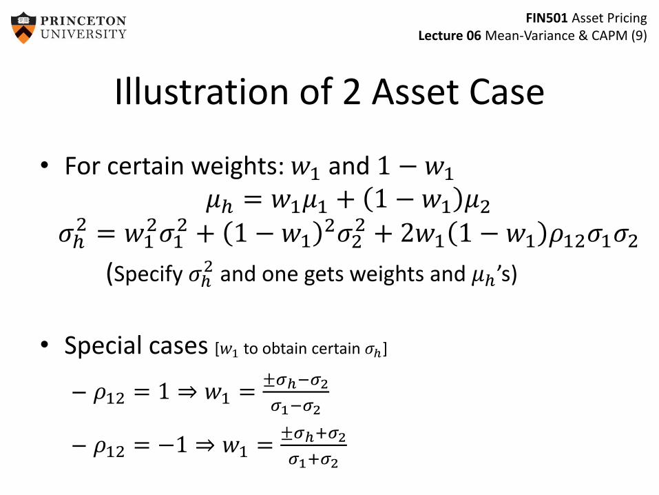
Illustration of 2 Asset Case
• For certain weights: 𝑤1 and 1 − 𝑤1
𝜇ℎ = 𝑤1𝜇1 + 1 − 𝑤1 𝜇2
𝜎ℎ2 = 𝑤1
2𝜎12 + 1 − 𝑤1
2𝜎22 + 2𝑤1 1 − 𝑤1 𝜌12𝜎1𝜎2
(Specify 𝜎ℎ2 and one gets weights and 𝜇ℎ’s)
• Special cases [𝑤1 to obtain certain 𝜎ℎ]
– 𝜌12 = 1 ⇒ 𝑤1 =±𝜎ℎ−𝜎2
𝜎1−𝜎2
– 𝜌12 = −1 ⇒ 𝑤1 =±𝜎ℎ+𝜎2
𝜎1+𝜎2

FIN501 Asset PricingLecture 06 Mean-Variance & CAPM (10)
For 𝜌12 = 1 ⇒ 𝑤1 =±𝜎ℎ−𝜎2
𝜎1−𝜎2
𝜎ℎ = 𝑤1𝜎1 + 1 − 𝑤1 𝜎2
𝜇ℎ = 𝑤1𝜇1 + 1 − 𝑤1 𝜇2 = 𝜇1 +𝜇2 − 𝜇1
𝜎2 − 𝜎1±𝜎ℎ − 𝜎1
Lower part is irrelevant
𝜇ℎ = 𝜇1 +𝜇2 − 𝜇1
𝜎2 − 𝜎1−𝜎ℎ − 𝜎1
The Efficient Frontier: Two Perfectly Correlated Risky Assets
𝜇2
𝜇1
𝜇ℎ
𝜎1 𝜎2𝜎ℎ

FIN501 Asset PricingLecture 06 Mean-Variance & CAPM (11)
For 𝜌12 = −1 ⇒ 𝑤1 =±𝜎𝑝+−𝜎2
𝜎1+𝜎2
𝜎ℎ = 𝑤1𝜎1 − 1 − 𝑤1 𝜎2
𝜇ℎ = 𝑤1𝜇1 + 1 − 𝑤1 𝜇2 =𝜎2
𝜎1 + 𝜎2𝜇1 +
𝜎1
𝜎1 + 𝜎2𝜇2 ±
𝜇2 − 𝜇1
𝜎1 + 𝜎2𝜎𝑝
The Efficient Frontier: Two Perfectly Negative Correlated Risky Assets
𝜇1
slope: 𝜇2−𝜇1
𝜎1+𝜎2
slope: −𝜇2−𝜇1
𝜎1+𝜎2
intercept: 𝜎2𝜎1+𝜎2
𝜇1+𝜎1
𝜎1+𝜎2𝜇2
𝜇2
𝜎1 𝜎2

FIN501 Asset PricingLecture 06 Mean-Variance & CAPM (12)
s1 s2
E[r2]
E[r1]
For 𝜌12 ∈ −1,1
The Efficient Frontier: Two Imperfectly Correlated Risky Assets

FIN501 Asset PricingLecture 06 Mean-Variance & CAPM (13)
For 𝜎1 = 0
The Efficient Frontier: One Risky and One Risk-Free Asset
𝜇2
𝜇1
𝜇ℎ
𝜎1 𝜎2𝜎ℎ

FIN501 Asset PricingLecture 06 Mean-Variance & CAPM (14)
Efficient frontier with n risky assets
• A frontier portfolio is one which displays minimum variance among all feasible portfolios with the same expected portfolio return.
• min𝒘
1
2𝒘′𝑉𝒘
– 𝜆: 𝒘′𝝁 = 𝜇ℎ, 𝑗 𝑤𝑗 𝔼 𝑟𝑖 = 𝜇ℎ
– 𝛾: 𝒘′𝟏 = 1, 𝑗 𝑤𝑗 = 1
• Result: Portfolio weights are linear in expected portfolio return 𝑤ℎ = 𝓰 + 𝓱𝜇ℎ
– If 𝜇ℎ = 0, 𝑤ℎ = 𝓰
– If 𝜇ℎ = 1, 𝑤ℎ = 𝓰 + 𝓱• Hence, 𝓰 and 𝓰 + 𝓱 are portfolios on the frontier
s
𝔼[𝑟]

FIN501 Asset PricingLecture 06 Mean-Variance & CAPM (15)
𝜕ℒ
𝜕𝑤= 𝑉𝒘 − 𝜆𝝁 − 𝛾𝟏 = 0
𝜕ℒ
𝜕𝜆= 𝜇ℎ − 𝒘′𝝁 = 0
𝜕ℒ
𝜕𝛾= 1 − 𝒘′𝟏 = 0
The first FOC can be written as:𝑉𝒘 = 𝜆𝝁 + 𝛾𝟏𝒘 = 𝜆𝑉−1𝝁 + 𝛾𝑉−1𝟏𝝁′𝒘 = 𝜆 𝝁′𝑉−1𝝁 + 𝛾 𝝁′𝑉−1𝟏 skip

FIN501 Asset PricingLecture 06 Mean-Variance & CAPM (16)
• Noting that 𝝁′𝒘ℎ = 𝑤ℎ′ , combining 1st and 2nd FOC
𝜇ℎ = 𝝁′𝒘ℎ = 𝜆 𝝁′𝑉−1𝝁𝐵
+ 𝛾 𝝁′𝑉−1𝟏𝐴
• Pre-multiplying the 1st FOC by 1 yields𝟏′𝒘ℎ = 𝒘ℎ
′ 𝟏 = 𝜆(𝟏′𝑉−1𝝁 + 𝛾 𝟏′𝑉−1𝟏 = 11 = 𝜆(𝟏′𝑉−1𝝁)
𝐴
+ 𝛾 𝟏′𝑉−1𝟏𝐶
• Solving for 𝜆, 𝛾
𝜆 =𝐶𝜇ℎ − 𝐴
𝐷, 𝛾 =
𝐵 − 𝐴𝜇ℎ
𝐷𝐷 = 𝐵𝐶 − 𝐴2
skip

FIN501 Asset PricingLecture 06 Mean-Variance & CAPM (17)
• Hence, 𝒘ℎ = 𝜆𝑉−1𝝁 + 𝛾𝑉−1𝟏 becomes
𝒘ℎ =𝐶𝜇ℎ − 𝐴
𝐷𝑉−1𝝁 +
𝐵 − 𝐴𝜇ℎ
𝐷𝑉−1𝟏
=1
𝐷𝐵 𝑉−1𝟏 − 𝐴 𝑉−1𝝁
𝓰
+1
𝐷𝐶 𝑉−1𝝁 − 𝐴 𝑉−1𝟏
𝓱
𝜇ℎ
• Result: Portfolio weights are linear in expected portfolio return 𝒘ℎ = 𝓰 + 𝓱𝜇ℎ
– If 𝜇ℎ = 0, 𝒘ℎ = 𝓰– If 𝜇ℎ= 1, 𝒘ℎ = 𝓰 + 𝓱
• Hence, 𝓰 and 𝓰 + 𝓱 are portfolios on the frontier
skip

FIN501 Asset PricingLecture 06 Mean-Variance & CAPM (18)
Characterization of Frontier Portfolios
• Proposition: The entire set of frontier portfolios canbe generated by ("are convex combinations" 𝓰 of)and 𝓰 + 𝓱.
• Proposition: The portfolio frontier can be describedas convex combinations of any two frontierportfolios, not just the frontier portfolios 𝓰 and 𝓰 +𝓱.
• Proposition: Any convex combination of frontierportfolios is also a frontier portfolio.
skip

FIN501 Asset PricingLecture 06 Mean-Variance & CAPM (19)
…Characterization of Frontier Portfolios…
• For any portfolio on the frontier,
𝜎2 𝜇ℎ = 𝓰 + 𝓱𝜇ℎ ′𝑉 𝓰 + 𝓱𝜇ℎ
with 𝓰 and 𝓱 as defined earlier.
Multiplying all this out and some algebra yields:
𝜎2 𝜇ℎ =𝐶
𝐷𝜇ℎ −
𝐴
𝐶
2
+1
𝐶
skip
FIN501 Asset PricingLecture 06 Mean-Variance & CAPM (20)
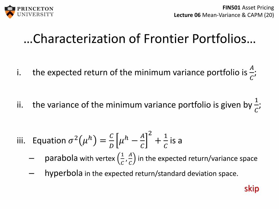
…Characterization of Frontier Portfolios…
i. the expected return of the minimum variance portfolio is𝐴
𝐶;
ii. the variance of the minimum variance portfolio is given by1
𝐶;
iii. Equation 𝜎2 𝜇ℎ =𝐶
𝐷𝜇ℎ −
𝐴
𝐶
2+
1
𝐶is a
– parabola with vertex1
𝐶,𝐴
𝐶in the expected return/variance space
– hyperbola in the expected return/standard deviation space.
skip

FIN501 Asset PricingLecture 06 Mean-Variance & CAPM (21)
Figure 6-3 The Set of Frontier Portfolios: Mean/Variance Space
𝐸 𝑟ℎ =𝐴
𝐶±
𝐷
𝐶𝜎2 −
1
𝐶

FIN501 Asset PricingLecture 06 Mean-Variance & CAPM (22)
Figure 6-4 The Set of Frontier Portfolios: Mean/SD Space

FIN501 Asset PricingLecture 06 Mean-Variance & CAPM (23)
Figure 6-5 The Set of Frontier Portfolios: Short Selling Allowed

FIN501 Asset PricingLecture 06 Mean-Variance & CAPM (24)
Efficient Frontier with risk-free asset
The Efficient Frontier: One Risk Free and n Risky Assets

FIN501 Asset PricingLecture 06 Mean-Variance & CAPM (25)
Efficient Frontier with risk-free asset
• min𝒘
1
2𝒘′𝑉𝒘
– s.t. 𝒘′𝝁 + 1 − 𝑤𝑇𝟏 𝑟𝑓 = 𝜇ℎ
– FOC
• 𝒘ℎ = 𝜆𝑉−1 𝝁 − 𝑟𝑓𝟏
• Multiplying by 𝝁 − 𝑟𝑓𝟏𝑇
yields 𝜆 =𝜇ℎ−𝑟𝑓
𝝁−𝑟𝑓𝟏′𝑉−1 𝝁−𝑟𝑓𝟏
– Solution
• 𝒘ℎ =𝑉−1 𝝁−𝑟𝑓𝟏 𝜇ℎ−𝑟𝑓
𝐻2 , where 𝐻 = 𝐵 − 2𝐴𝑟𝑓 + 𝐶(𝑟𝑓)2

FIN501 Asset PricingLecture 06 Mean-Variance & CAPM (26)
Efficient frontier with risk-free asset
• Result 1: Excess return in frontier excess return
cov 𝑟ℎ, 𝑟𝑝 = 𝒘ℎ′ 𝑉𝒘𝑝 = 𝒘ℎ
′ 𝝁 − 𝑟𝑓𝟏𝐸 𝑟𝑝 − 𝑟𝑓
𝐻2
=𝐸 𝑟ℎ − 𝑟𝑓 𝐸 𝑟𝑝 − 𝑟𝑓
𝐻2
var 𝑟𝑝 =𝐸 𝑟𝑝 − 𝑟𝑓 2
𝐻2
𝐸 𝑟ℎ − 𝑟𝑓 =cov 𝑟ℎ, 𝑟𝑝
var 𝑟𝑝𝛽ℎ,𝑝
𝐸 𝑟𝑝 − 𝑟𝑓
(Holds for any frontier portfolio 𝑝, in particular the market portfolio)

FIN501 Asset PricingLecture 06 Mean-Variance & CAPM (27)
Efficient Frontier with risk-free asset
• Result 2: Frontier is linear in 𝐸 𝑟 , 𝜎 -space
var 𝑟ℎ =𝐸 𝑟ℎ − 𝑟𝑓
2
𝐻2
𝐸 𝑟ℎ = 𝑟𝑓 + 𝐻𝜎ℎ
where 𝐻 is the Sharpe ratio
𝐻 =𝐸 𝑟ℎ − 𝑟𝑓
𝜎ℎ

FIN501 Asset PricingLecture 06 Mean-Variance & CAPM (28)
Overview
1. Introduction: Simple CAPM with quadratic utility functions
2. Traditional Derivation of CAPM– Demand: Portfolio Theory – Aggregation: Fund Separation Theorem– Equilibrium: CAPM
3. Modern Derivation of CAPM– Projections– Pricing Kernel and Expectation Kernel
4. Testing CAPM5. Practical Issues – Black-Litterman
for given prices/returns

FIN501 Asset PricingLecture 06 Mean-Variance & CAPM (29)
Aggregation: Two Fund Separation
• Doing it in two steps:
– First solve frontier for n risky asset
– Then solve tangency point
• Advantage:
– Same portfolio of n risky asset for different agents with different risk aversion
– Useful for applying equilibrium argument (later)
Recall HARA class of preferences

FIN501 Asset PricingLecture 06 Mean-Variance & CAPM (30)
Optimal Portfolios of Two Investors with Different Risk Aversion
Two Fund Separation
Price of Risk == highest
Sharpe ratio

FIN501 Asset PricingLecture 06 Mean-Variance & CAPM (31)
Mean-Variance Preferences
• 𝑈 𝜇ℎ, 𝜎ℎ with 𝜕𝑈
𝜕𝜇ℎ> 0,
𝜕𝑈
𝜕𝜎ℎ2 < 0
– Example: 𝐸 𝑊 −𝜌
2var 𝑊
• Also in expected utility framework– Example 1: Quadratic utility function (with portfolio return 𝑅)
• 𝑈 𝑅 = 𝑎 + 𝑏𝑅 + 𝑐𝑅2
• vNM: 𝐸 𝑈 𝑅 = 𝑎 + 𝑏𝐸 𝑅 + 𝑐𝐸 𝑅2 = 𝑎 + 𝑏𝜇ℎ + 𝑐𝜇ℎ2 + 𝑐𝜎ℎ
2 =𝑔 𝜇ℎ, 𝜎ℎ
– Example 2: CARA Gaussian• asset returns jointly normal ⇒ 𝑖 𝑤𝑖𝑟𝑖 normal
• If 𝑈 is CARA ⇒ certainty equivalent is 𝜇ℎ −𝜌
2𝜎ℎ
2

FIN501 Asset PricingLecture 06 Mean-Variance & CAPM (32)
Overview
1. Introduction: Simple CAPM with quadratic utility functions
2. Traditional Derivation of CAPM– Demand: Portfolio Theory – Aggregation: Fund Separation Theorem– Equilibrium: CAPM
3. Modern Derivation of CAPM– Projections– Pricing Kernel and Expectation Kernel
4. Testing CAPM5. Practical Issues – Black-Litterman
for given prices/returns

FIN501 Asset PricingLecture 06 Mean-Variance & CAPM (33)
Equilibrium leads to CAPM
• Portfolio theory: only analysis of demand– price/returns are taken as given
– composition of risky portfolio is same for all investors
• Equilibrium Demand = Supply (market portfolio)
• CAPM allows to derive– equilibrium prices/ returns.
– risk-premium

FIN501 Asset PricingLecture 06 Mean-Variance & CAPM (34)
The CAPM with a risk-free bond
• The market portfolio is efficient since it is on the efficient frontier.
• All individual optimal portfolios are located on the half-line originating at point (0, 𝑟𝑓).
• The slope of Capital Market Line (CML):𝐸 𝑅𝑚𝑘𝑡 −𝑅𝑓
𝜎𝑚𝑘𝑡
𝐸 𝑅ℎ = 𝑅𝑓 +𝐸 𝑅𝑚𝑘𝑡 − 𝑅𝑓
𝜎𝑚𝑘𝑡𝜎ℎ
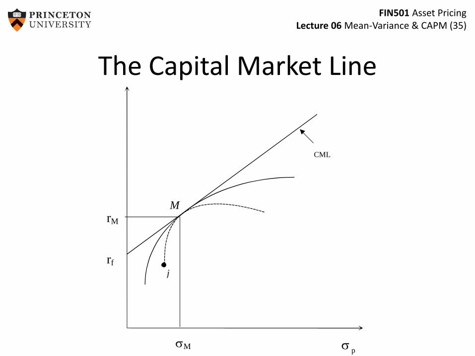
FIN501 Asset PricingLecture 06 Mean-Variance & CAPM (35)
sp
j
MrM
sM
rf
CML
The Capital Market Line

FIN501 Asset PricingLecture 06 Mean-Variance & CAPM (36)
The Security Market Line
bbi
bM
= 1
rf
E(rM
)
E(ri)
E(r)
slope SML = (E(ri)-r
f) /b
i
SML
FIN501 Asset PricingLecture 06 Mean-Variance & CAPM (37)
Overview
1. Introduction: Simple CAPM with quadratic utility functions
2. Traditional Derivation of CAPM– Demand: Portfolio Theory
– Aggregation: Fund Separation Theorem
– Equilibrium: CAPM
3. Modern Derivation of CAPM– Projections
– Pricing Kernel and Expectation Kernel
4. Practical Issues
for given prices/returns
FIN501 Asset PricingLecture 06 Mean-Variance & CAPM (38)
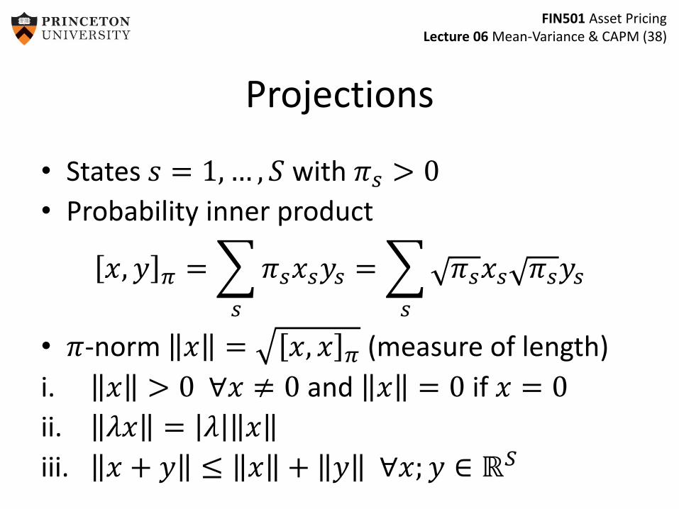
Projections
• States 𝑠 = 1, … , 𝑆 with 𝜋𝑠 > 0
• Probability inner product
𝑥, 𝑦 𝜋 =
𝑠
𝜋𝑠𝑥𝑠𝑦𝑠 =
𝑠
𝜋𝑠𝑥𝑠 𝜋𝑠𝑦𝑠
• 𝜋-norm 𝑥 = 𝑥, 𝑥 𝜋 (measure of length)
i. 𝑥 > 0 ∀𝑥 ≠ 0 and 𝑥 = 0 if 𝑥 = 0
ii. 𝜆𝑥 = 𝜆 𝑥
iii. 𝑥 + 𝑦 ≤ 𝑥 + 𝑦 ∀𝑥; 𝑦 ∈ ℝ𝑆

FIN501 Asset PricingLecture 06 Mean-Variance & CAPM (39)
)shrinkaxes
x x
y y
x and y are 𝜋-orthogonal iff 𝑥, 𝑦 𝜋 = 0, i.e. 𝐸 𝑥𝑦 = 0
FIN501 Asset PricingLecture 06 Mean-Variance & CAPM (40)
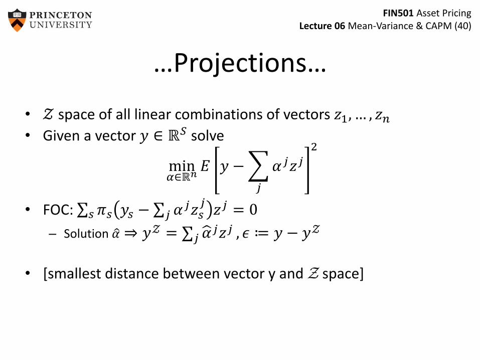
…Projections…
• 𝒵 space of all linear combinations of vectors 𝑧1, … , 𝑧𝑛
• Given a vector 𝑦 ∈ ℝ𝑆 solve
min𝛼∈ℝ𝑛
𝐸 𝑦 −
𝑗
𝛼𝑗𝑧𝑗
2
• FOC: 𝑠 𝜋𝑠 𝑦𝑠 − 𝑗 𝛼𝑗𝑧𝑠𝑗
𝑧𝑗 = 0
– Solution 𝛼 ⇒ 𝑦𝒵 = 𝑗 𝛼𝑗𝑧𝑗 , 𝜖 ≔ 𝑦 − 𝑦𝒵
• [smallest distance between vector y and Z space]
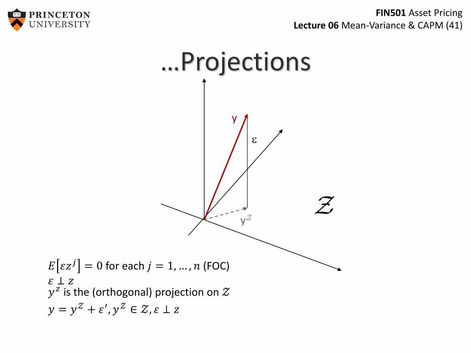
FIN501 Asset PricingLecture 06 Mean-Variance & CAPM (41)
y
yZ
e
𝐸 𝜀𝑧𝑗 = 0 for each 𝑗 = 1, … , 𝑛 (FOC)
𝜀 ⊥ 𝑧𝑦𝑧 is the (orthogonal) projection on 𝒵
𝑦 = 𝑦𝒵 + 𝜀′, 𝑦𝒵 ∈ 𝒵, 𝜀 ⊥ 𝑧
…Projections

FIN501 Asset PricingLecture 06 Mean-Variance & CAPM (42)
Expected Value and Co-Variance…squeeze axis by 𝜋𝑠
x
(1,1)
𝑥, 𝑦 = 𝐸 𝑥𝑦 = cov 𝑥, 𝑦 + 𝐸 𝑥 𝐸 𝑦𝑥, 𝑥 = 𝐸 𝑥2 = var 𝑥 + 𝐸 𝑥 2
𝑥 = 𝐸 𝑥2
𝑥 = 𝑥 + 𝑥
𝑥
𝑥

FIN501 Asset PricingLecture 06 Mean-Variance & CAPM (43)
…Expected Value and Co-Variance
• 𝑥 = 𝑥 + 𝑥 where – 𝑥 is a projection of 𝑥 onto 1
– 𝑥 is a projection of 𝑥 onto 1 ⊥
• 𝐸 𝑥 = 𝑥, 1 𝜋 = 𝑥, 1 𝜋 = 𝑥 1,1 𝜋 = 𝑥
• var 𝑥 = 𝑥, 𝑥 𝜋 = var[ 𝑥]
– 𝜎𝑥 = 𝑥 𝜋
• cov 𝑥, 𝑦 = cov 𝑥, 𝑦 = 𝑥, 𝑦 𝜋
• Proof: 𝑥, 𝑦 𝜋 = 𝑥, 𝑦 𝜋 + 𝑥, 𝑦 𝜋
– 𝑦, 𝑥 𝜋 = 𝑦, 𝑥 𝜋 = 0, 𝑥, 𝑦 𝜋 = 𝐸 𝑦 𝐸 𝑥 + cov[ 𝑥, 𝑦]
scalar slight abuse of notation

FIN501 Asset PricingLecture 06 Mean-Variance & CAPM (44)
Overview
1. Introduction: Simple CAPM with quadratic utility functions
2. Traditional Derivation of CAPM– Demand: Portfolio Theory – Aggregation: Fund Separation Theorem– Equilibrium: CAPM
3. Modern Derivation of CAPM– Projections– Pricing Kernel and Expectation Kernel
4. Testing CAPM5. Practical Issues – Black-Litterman
for given prices/returns
FIN501 Asset PricingLecture 06 Mean-Variance & CAPM (45)
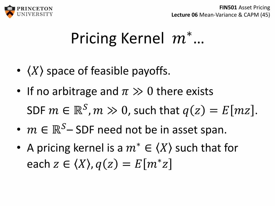
Pricing Kernel 𝑚∗…
• 𝑋 space of feasible payoffs.
• If no arbitrage and 𝜋 ≫ 0 there exists
SDF 𝑚 ∈ ℝ𝑆, 𝑚 ≫ 0, such that 𝑞 𝑧 = 𝐸 𝑚𝑧 .
• 𝑚 ∈ ℝ𝑆– SDF need not be in asset span.
• A pricing kernel is a 𝑚∗ ∈ 𝑋 such that for
each 𝑧 ∈ 𝑋 , 𝑞 𝑧 = 𝐸 𝑚∗𝑧

FIN501 Asset PricingLecture 06 Mean-Variance & CAPM (46)
…Pricing Kernel - Examples…
• Example 1:
– 𝑆 = 3, 𝜋𝑠 =1
3
– 𝑥1 = 1,0,0 , 𝑥2 = 0,1,1 and 𝑝 =1
3,2
3
– Then 𝑚∗ = 1,1,1 is the unique pricing kernel.
• Example 2:
– 𝑥1 = 1,0,0 , 𝑥2 = 0,1,0 , 𝑝 =1
3,2
3
– Then 𝑚∗ = 1,2,0 is the unique pricing kernel.

FIN501 Asset PricingLecture 06 Mean-Variance & CAPM (47)
…Pricing Kernel – Uniqueness
• If a state price density exists, there exists a unique pricing kernel.
– If dim 𝑋 = 𝑆 (markets are complete), there are exactly 𝑚 equations and 𝑚 unknowns
– If dim 𝑋 < 𝑆, (markets may be incomplete)
For any state price density (=SDF) 𝑚 and any 𝑧 ∈ 𝑋
𝐸 𝑚 − 𝑚∗ 𝑧 = 0
𝑚 = 𝑚 − 𝑚∗ + 𝑚∗ ⇒ 𝑚∗is the “projection” of 𝑚
on 𝑋• Complete markets ⇒ 𝑚∗ = 𝑚 (SDF=state price density)

FIN501 Asset PricingLecture 06 Mean-Variance & CAPM (48)
Expectations Kernel 𝑘∗
• An expectations kernel is a vector 𝑘∗ ∈ 𝑋
– Such that 𝐸 𝑧 = 𝐸 𝑘∗𝑧 for each 𝑧 ∈ 𝑋
• Example
– 𝑆 = 3, 𝜋𝑠 =1
3, 𝑥1 = 1,0,0 , 𝑥2 = 0,1,0
– Then the unique 𝑘∗ = 1,1,0
• If 𝜋 ≫ 0, there exists a unique expectations kernel.
• Let 𝐼 = 1, … , 1 then for any 𝑧 ∈ 𝑋𝐸 𝐼 − 𝑘∗ 𝑧 = 0
– 𝑘∗is the “projection” of 𝐼 on 𝑋– 𝑘∗ = 𝐼 if bond can be replicated (e.g. if markets are complete)
FIN501 Asset PricingLecture 06 Mean-Variance & CAPM (49)
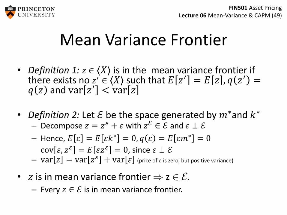
Mean Variance Frontier
• Definition 1: 𝑧 ∈ 𝑋 is in the mean variance frontier if there exists no 𝑧′ ∈ 𝑋 such that 𝐸 𝑧′ = 𝐸 𝑧 , 𝑞 𝑧′ =𝑞 𝑧 and var 𝑧′ < var 𝑧
• Definition 2: Let ℰ be the space generated by 𝑚∗and 𝑘∗
– Decompose 𝑧 = 𝑧𝜀 + 𝜀 with 𝑧ℰ ∈ ℰ and 𝜀 ⊥ ℰ
– Hence, 𝐸 𝜀 = 𝐸 𝜀𝑘∗ = 0, 𝑞 𝜀 = 𝐸 𝜀𝑚∗ = 0
cov 𝜀, 𝑧𝜀 = 𝐸 𝜀𝑧𝜀 = 0, since 𝜀 ⊥ ℰ– var 𝑧 = var 𝑧𝜀 + var 𝜀 (price of 𝜀 is zero, but positive variance)
• 𝑧 is in mean variance frontier ) z 2 E.– Every 𝑧 ∈ ℰ is in mean variance frontier.

FIN501 Asset PricingLecture 06 Mean-Variance & CAPM (50)
Frontier Returns…
• Frontier returns are the returns of frontier payoffs with non-zero prices.
[Note: R indicates Gross return]
𝑅𝑘∗ =𝑘∗
𝑞 𝑘∗=
𝑘∗
𝐸 𝑚∗
𝑅𝑚∗ =𝑚∗
𝑞 𝑚∗=
𝑚∗
𝐸 𝑚∗𝑚∗
• If 𝑧 = 𝛼𝑚∗ + 𝛽𝑘∗ then
𝑅𝑧 =𝛼𝑞 𝑚∗
𝛼𝑞 𝑚∗ + 𝛽𝑞 𝑘∗
𝜆
𝑅𝑚∗ +𝛽𝑞 𝑘∗
𝛼𝑞 𝑚∗ + 𝛽𝑞 𝑘∗
1−𝜆
𝑅𝑘∗
• graphically: payoffs with price of p=1.

FIN501 Asset PricingLecture 06 Mean-Variance & CAPM (51)
𝑚∗
Mean-Variance Return Frontierp=1-line = return-line (orthogonal to 𝑚∗)
𝑋 = RS = R3
Mean-Variance Payoff Frontier
e

FIN501 Asset PricingLecture 06 Mean-Variance & CAPM (52)
0𝑚∗
(1,1,1)
expected return
standard deviation
Mean-Variance (Payoff) Frontier
NB: graphical illustrated of expected returns and standard deviation changes if bond is not in payoff span.
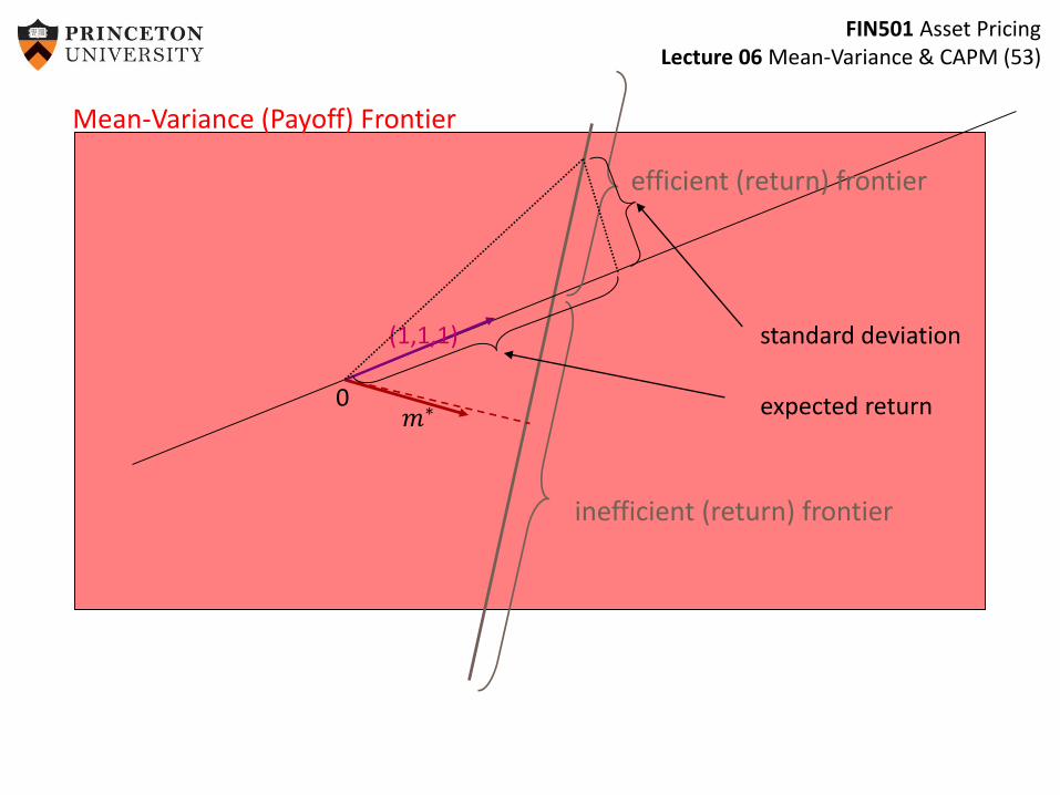
FIN501 Asset PricingLecture 06 Mean-Variance & CAPM (53)
0𝑚∗
(1,1,1)
inefficient (return) frontier
efficient (return) frontier
expected return
standard deviation
Mean-Variance (Payoff) Frontier
FIN501 Asset PricingLecture 06 Mean-Variance & CAPM (54)
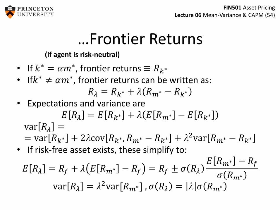
…Frontier Returns
• If 𝑘∗ = 𝛼𝑚∗, frontier returns ≡ 𝑅𝑘∗
• If𝑘∗ ≠ 𝛼𝑚∗, frontier returns can be written as:𝑅𝜆 = 𝑅𝑘∗ + 𝜆 𝑅𝑚∗ − 𝑅𝑘∗
• Expectations and variance are𝐸 𝑅𝜆 = 𝐸 𝑅𝑘∗ + 𝜆 𝐸 𝑅𝑚∗ − 𝐸 𝑅𝑘∗
var 𝑅𝜆 == var 𝑅𝑘∗ + 2𝜆cov 𝑅𝑘∗ , 𝑅𝑚∗ − 𝑅𝑘∗ + 𝜆2var 𝑅𝑚∗ − 𝑅𝑘∗
• If risk-free asset exists, these simplify to:
𝐸 𝑅𝜆 = 𝑅𝑓 + 𝜆 𝐸 𝑅𝑚∗ − 𝑅𝑓 = 𝑅𝑓 ± 𝜎 𝑅𝜆
𝐸 𝑅𝑚∗ − 𝑅𝑓
𝜎 𝑅𝑚∗
var 𝑅𝜆 = 𝜆2var[𝑅𝑚∗] , 𝜎 𝑅𝜆 = 𝜆 𝜎 𝑅𝑚∗
(if agent is risk-neutral)
FIN501 Asset PricingLecture 06 Mean-Variance & CAPM (55)
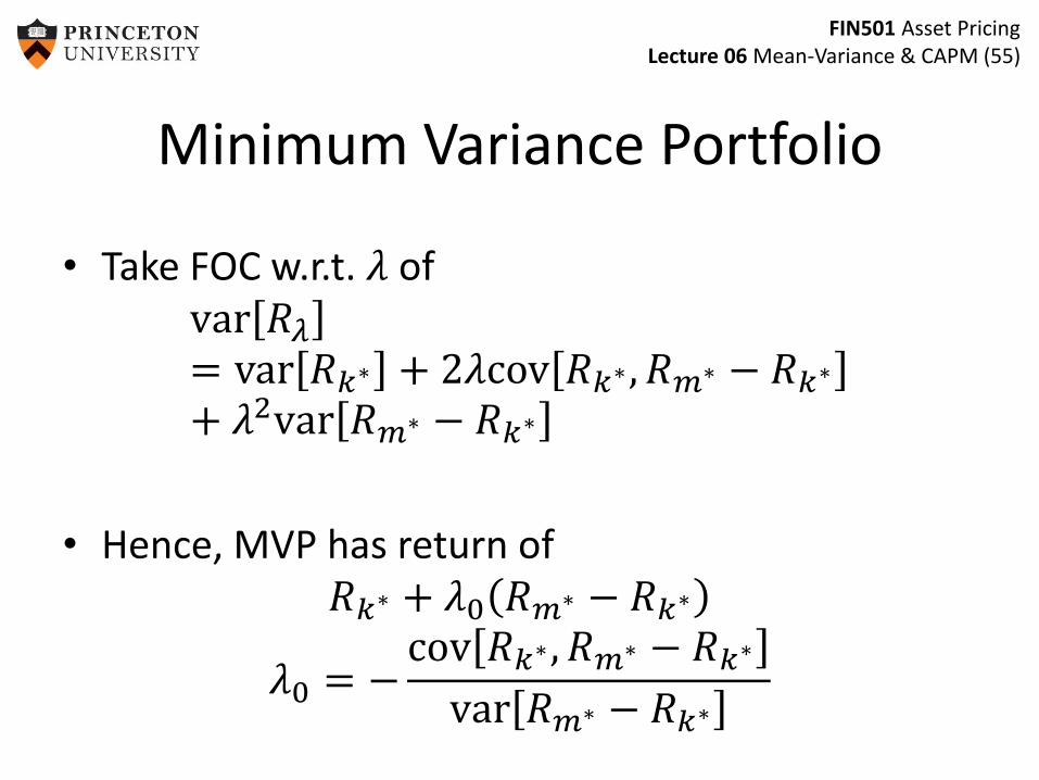
Minimum Variance Portfolio
• Take FOC w.r.t. 𝜆 ofvar 𝑅𝜆
= var 𝑅𝑘∗ + 2𝜆cov 𝑅𝑘∗ , 𝑅𝑚∗ − 𝑅𝑘∗
+ 𝜆2var 𝑅𝑚∗ − 𝑅𝑘∗
• Hence, MVP has return of𝑅𝑘∗ + 𝜆0 𝑅𝑚∗ − 𝑅𝑘∗
𝜆0 = −cov 𝑅𝑘∗ , 𝑅𝑚∗ − 𝑅𝑘∗
var 𝑅𝑚∗ − 𝑅𝑘∗

FIN501 Asset PricingLecture 06 Mean-Variance & CAPM (56)
(1,1,1)
Illustration of MVP
Minimum standard deviation
Expected return of MVP
𝑋 = ℝ2 and 𝑆 = 3
FIN501 Asset PricingLecture 06 Mean-Variance & CAPM (57)
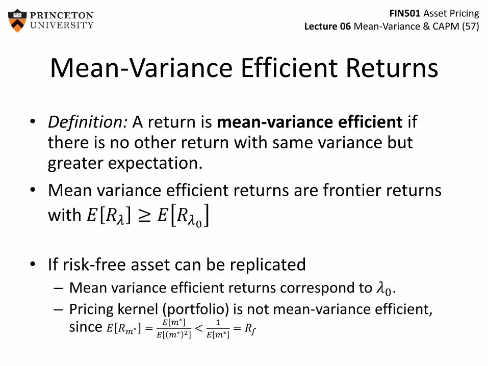
Mean-Variance Efficient Returns
• Definition: A return is mean-variance efficient if there is no other return with same variance but greater expectation.
• Mean variance efficient returns are frontier returns
with 𝐸 𝑅𝜆 ≥ 𝐸 𝑅𝜆0
• If risk-free asset can be replicated– Mean variance efficient returns correspond to 𝜆0.
– Pricing kernel (portfolio) is not mean-variance efficient, since 𝐸 𝑅𝑚∗ =
𝐸 𝑚∗
𝐸 𝑚∗ 2 <1
𝐸 𝑚∗ = 𝑅𝑓

FIN501 Asset PricingLecture 06 Mean-Variance & CAPM (58)
Zero-Covariance Frontier Returns
• Take two frontier portfolios with returns𝑅𝜆 = 𝑅𝑘∗ + 𝜆 𝑅𝑚∗ − 𝑅𝑘∗ and 𝑅𝜇 = 𝑅𝑘∗ + 𝜇 𝑅𝑚∗ − 𝑅𝑘∗
• cov 𝑅𝜇 , 𝑅𝜆 = var 𝑅𝑘∗ + 𝜆 + 𝜇 cov 𝑅𝑘∗ , 𝑅𝑚∗ − 𝑅𝑘∗ +𝜆𝜇var 𝑅𝑚∗ − 𝑅𝑘∗
• The portfolios have zero co-variance if
𝜇 = −var 𝑅𝑘∗ + 𝜆cov 𝑅𝑘∗ , 𝑅𝑚∗ − 𝑅𝑘∗
cov 𝑅𝑘∗ , 𝑅𝑚∗ − 𝑅𝑘∗ + 𝜆var 𝑅𝑚∗ − 𝑅𝑘∗
• For all 𝜆 ≠ 𝜆0, 𝜇 exists– 𝜇 = 0 if risk-free bond can be replicated

FIN501 Asset PricingLecture 06 Mean-Variance & CAPM (59)
(1,1,1)
Illustration of ZC Portfolio…
arbitrary portfolio p
Recall:
cov 𝑥, 𝑦 = 𝑥, 𝑦 𝜋
𝑋 = ℝ2 and 𝑆 = 3

FIN501 Asset PricingLecture 06 Mean-Variance & CAPM (60)
(1,1,1)
…Illustration of ZC Portfolio
arbitrary portfolio p
ZC of p
Green lines do not necessarily cross.
FIN501 Asset PricingLecture 06 Mean-Variance & CAPM (61)
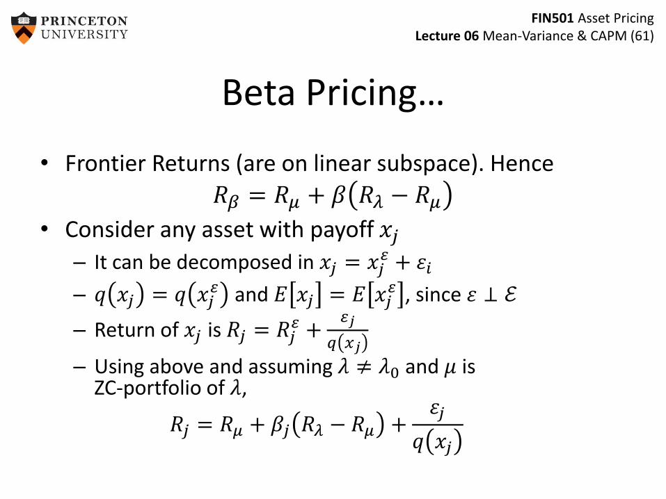
Beta Pricing…
• Frontier Returns (are on linear subspace). Hence
𝑅𝛽 = 𝑅𝜇 + 𝛽 𝑅𝜆 − 𝑅𝜇
• Consider any asset with payoff 𝑥𝑗
– It can be decomposed in 𝑥𝑗 = 𝑥𝑗𝜀 + 𝜀𝑖
– 𝑞 𝑥𝑗 = 𝑞 𝑥𝑗𝜀 and 𝐸 𝑥𝑗 = 𝐸 𝑥𝑗
𝜀 , since 𝜀 ⊥ ℰ
– Return of 𝑥𝑗 is 𝑅𝑗 = 𝑅𝑗𝜀 +
𝜀𝑗
𝑞 𝑥𝑗
– Using above and assuming 𝜆 ≠ 𝜆0 and 𝜇 is ZC-portfolio of 𝜆,
𝑅𝑗 = 𝑅𝜇 + 𝛽𝑗 𝑅𝜆 − 𝑅𝜇 +𝜀𝑗
𝑞 𝑥𝑗

FIN501 Asset PricingLecture 06 Mean-Variance & CAPM (62)
…Beta Pricing
• Taking expectations and deriving covariance
• 𝐸 𝑅𝑗 = 𝐸 𝑅𝜇 + 𝛽𝑗 𝐸 𝑅𝜆 − 𝐸 𝑅𝜇
• cov 𝑅𝜆, 𝑅𝑗 = 𝛽𝑗var 𝑅𝜆 ⇒ 𝛽𝑗 =cov 𝑅𝜆,𝑅𝑗
var 𝑅𝜆
– Since 𝑅𝜆 ⊥𝜀𝑗
𝑞 𝑥𝑗
• If risk-free asset can be replicated, beta-pricing equation simplifies to
𝐸 𝑅𝑗 = 𝑅𝑓 + 𝛽𝑗 𝐸 𝑅𝜆 − 𝑅𝑓
• Problem: How to identify frontier returns

FIN501 Asset PricingLecture 06 Mean-Variance & CAPM (63)
Capital Asset Pricing Model…
• CAPM = market return is frontier return– Derive conditions under which market return is frontier return
– Two periods: 0,1.
– Endowment: individual 𝑤1𝑖 at time 1, aggregate 𝑤1 = 𝑤1
𝑋 +
𝑤1𝑌 , where 𝑤1
𝑋 , 𝑤1𝑌 are orthogonal and 𝑤1
𝑋 is the
orthogonal projection of 𝑤1 on 𝑋 .
– The market payoff is 𝑤1𝑋
– Assume 𝑞 𝑤1𝑋 ≠ 0, let 𝑅𝑚𝑘𝑡 =
𝑤1𝑋
𝑞 𝑤1𝑋 , and assume that
𝑅𝑚𝑘𝑡 is not the minimum variance return.

FIN501 Asset PricingLecture 06 Mean-Variance & CAPM (64)
…Capital Asset Pricing Model
• If 𝑅0 is the frontier return that has zero covariance with 𝑅𝑚𝑘𝑡 then, for every security j,
• 𝐸 𝑅𝑗 = 𝐸 𝑅0 + 𝛽𝑗 𝐸 𝑅𝑚𝑘𝑡 − 𝐸 𝑅0 with
𝛽𝑗 =cov 𝑅𝑗,𝑅𝑚𝑘𝑡
var 𝑅𝑚𝑘𝑡
• If a risk free asset exists, equation becomes, 𝐸[𝑅𝑗] = 𝑅𝑓 + 𝛽𝑗 𝐸 𝑅𝑚𝑘𝑡 − 𝑅𝑓
• N.B. first equation always hold if there are only two assets.

FIN501 Asset PricingLecture 06 Mean-Variance & CAPM (65)
Overview
1. Introduction: Simple CAPM with quadratic utility functions
2. Traditional Derivation of CAPM– Demand: Portfolio Theory – Aggregation: Fund Separation Theorem– Equilibrium: CAPM
3. Modern Derivation of CAPM– Projections– Pricing Kernel and Expectation Kernel
4. Testing CAPM5. Practical Issues – Black-Litterman
for given prices/returns

FIN501 Asset PricingLecture 06 Mean-Variance & CAPM (66)
Practical Issues
• Testing of CAPM
• Jumping weights
– Domestic investments
– International investment
• Black-Litterman solution

FIN501 Asset PricingLecture 06 Mean-Variance & CAPM (67)
Testing the CAPM
• Take CAPM as given and test empirical implications
• Time series approach– Regress individual returns on market returns
𝑅𝑖𝑡 − 𝑅𝑓𝑡 = 𝛼𝑖 + 𝛽𝑖𝑚 𝑅𝑚𝑡 − 𝑅𝑓𝑡 + 𝜀𝑖𝑡
– Test whether constant term 𝛼𝑖 = 0
• Cross sectional approach– Estimate betas from time series regression– Regress individual returns on betas
𝑅𝑖 = 𝜆 𝛽𝑖𝑚 + 𝛼𝑖
– Test whether regression residuals 𝛼𝑖 = 0
FIN501 Asset PricingLecture 06 Mean-Variance & CAPM (68)
Empirical Evidence
• Excess returns on high-beta stocks are low
• Excess returns are high for small stocks
– Effect has been weak since early 1980s
• Value stocks have high returns despite low betas
• Momentum stocks have high returns and low betas

FIN501 Asset PricingLecture 06 Mean-Variance & CAPM (69)
Reactions and Critiques
• Roll Critique– The CAPM is not testable because composition of true
market portfolio is not observable
• Hansen-Richard Critique– The CAPM could hold conditionally at each point in
time, but fail unconditionally
• Anomalies are result of “data mining”
• Anomalies are concentrated in small, illiquid stocks
• Markets are inefficient – “joint hypothesis test”
FIN501 Asset PricingLecture 06 Mean-Variance & CAPM (70)
Practical Issues
• Estimation– How do we estimate all the parameters we need for
portfolio optimization?
• What is the market portfolio?– Restricted short-sales and other restrictions– International assets & currency risk
• How does the market portfolio change over time?– Empirical evidence– More in dynamic models

FIN501 Asset PricingLecture 06 Mean-Variance & CAPM (71)
Overview
1. Introduction: Simple CAPM with quadratic utility functions
2. Traditional Derivation of CAPM– Demand: Portfolio Theory – Aggregation: Fund Separation Theorem– Equilibrium: CAPM
3. Modern Derivation of CAPM– Projections– Pricing Kernel and Expectation Kernel
4. Testing CAPM5. Practical Issues – Black Litterman
for given prices/returns
FIN501 Asset PricingLecture 06 Mean-Variance & CAPM (72)
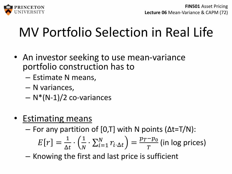
MV Portfolio Selection in Real Life
• An investor seeking to use mean-variance portfolio construction has to– Estimate N means,– N variances,– N*(N-1)/2 co-variances
• Estimating means– For any partition of [0,T] with N points (∆t=T/N):
𝐸 𝑟 =1
Δ𝑡⋅
1
𝑁⋅ 𝑖=1
𝑁 𝑟𝑖⋅Δ𝑡 =𝑝𝑇−𝑝0
𝑇(in log prices)
– Knowing the first and last price is sufficient

FIN501 Asset PricingLecture 06 Mean-Variance & CAPM (73)
Estimating Means
• Let 𝑋𝑘 denote the logarithmic return on the market, with 𝑘 =1, … , 𝑛 over a period of length ℎ– The dynamics to be estimated are:
𝑋𝑘 = 𝜇 ⋅ Δ + 𝜎 ⋅ Δ ⋅ 𝜖𝑘
where the 𝜖𝑘are i.i.d. standard normal random variables.– The standard estimator for the expected logarithmic mean rate of
return is:
𝜇 =1
ℎ⋅
1
𝑛
𝑋𝑘
– The mean and variance of this estimator
𝐸 𝜇 =1
ℎ⋅ 𝐸
1
𝑛
𝑋𝑘 =1
ℎ⋅ 𝑛 ⋅ 𝜇 ⋅ Δ = 𝜇
𝑉𝑎𝑟 𝜇 =1
ℎ2⋅ 𝑉𝑎𝑟
1
𝑛
𝑋𝑘 =1
ℎ2⋅ 𝑛 ⋅ 𝜎2 ⋅ Δ =
𝜎2
ℎ– The accuracy of the estimator depends only upon the total length of the observation period (h), and not upon the number of
observations (n).
where ℎ is length of observation𝑛 number of observationsΔ = 𝑛/ℎ

FIN501 Asset PricingLecture 06 Mean-Variance & CAPM (74)
Estimating Variances
• Consider the following estimator: 𝜎2 =
1
ℎ⋅ 𝑖=1
𝑛 𝑋𝑘2
• The mean and variance of this estimator:
𝐸 𝜎2 =1
ℎ⋅
𝑖=1
𝑛
𝐸 𝑋𝑘2 =
1
ℎ⋅ 𝑛 ⋅ 𝜇2 ⋅ Δ2 + 𝜎2 ⋅ Δ = 𝜎2 + 𝜇2 ⋅
ℎ
𝑛
𝑉𝑎𝑟 𝜎2 =1
ℎ2⋅ 𝑉𝑎𝑟
𝑖=1
𝑛
𝑋𝑘2 =
1
ℎ2⋅
𝑖=1
𝑛
𝑉𝑎𝑟 𝑋𝑘2 =
𝑛
ℎ2⋅ 𝐸 𝑋𝑘
4 − 𝐸 𝑋𝑘2 2
=2 ⋅ 𝜎4
𝑛+
4 ⋅ 𝜇2 ⋅ ℎ
𝑛2
– The estimator is biased b/c we did not subtract out the expected return from each realization.
– Magnitude of the bias declines as n increases. – For a fixed h, the accuracy of the variance estimator can be
improved by sampling the data more frequently.

FIN501 Asset PricingLecture 06 Mean-Variance & CAPM (75)
Estimating variances:Theory vs. Practice
• For any partition of [0, 𝑇] with 𝑁 points (Δ𝑡 = 𝑇/𝑁):
𝑉𝑎𝑟 𝑟 =1
𝑁⋅
𝑖=1
𝑁
𝑟𝑖⋅Δ𝑡 − 𝐸 𝑟 2 → 𝜎2 𝑎𝑠 𝑁 → ∞
• Theory: Observing the same time series at progressively higher frequencies increases the precision of the estimate.
• Practice:– Over shorter interval increments are non-Gaussian
– Volatility is time-varying (GARCH, SV-models)
– Market microstructure noise

FIN501 Asset PricingLecture 06 Mean-Variance & CAPM (76)
Estimating covariances:Theory vs. Practice
• In theory, the estimation of covariances shares the features of variance estimation.
• In practice:– Difficult to obtain synchronously observed time-series -> may require
interpolation, which affects the covariance estimates.
– The number of covariances to be estimated grows very quickly, such that the resulting covariance matrices are unstable (check condition numbers!).
– Shrinkage estimators (Ledoit and Wolf, 2003, “Honey, I Shrunk the Covariance Matrix”)

FIN501 Asset PricingLecture 06 Mean-Variance & CAPM (77)
Unstable Portfolio Weights
• Are optimal weights statistically different from zero?– Properly designed regression yields portfolio weights
– Statistical tests for significance of weight
• Example: Britton-Jones (1999) for international portfolio– Fully hedged USD Returns
• Period: 1977-1966
• 11 countries
– Results• Weights vary significantly across time and in the cross section
• Standard errors on coefficients tend to be large

FIN501 Asset PricingLecture 06 Mean-Variance & CAPM (78)
Britton-Jones (1999)1977-1996 1977-1986 1987-1996
weights t-stats weights t-stats weights t-stats
Australia 12.8 0.54 6.8 0.20 21.6 0.66
Austria 3.0 0.12 -9.7 -0.22 22.5 0.74
Belgium 29.0 0.83 7.1 0.15 66 1.21
Canada -45.2 -1.16 -32.7 -0.64 -68.9 -1.10
Denmark 14.2 0.47 -29.6 -0.65 68.8 1.78
France 1.2 0.04 -0.7 -0.02 -22.8 -0.48
Germany -18.2 -0.51 9.4 0.19 -58.6 -1.13
Italy 5.9 0.29 22.2 0.79 -15.3 -0.52
Japan 5.6 0.24 57.7 1.43 -24.5 -0.87
UK 32.5 1.01 42.5 0.99 3.5 0.07
US 59.3 1.26 27.0 0.41 107.9 1.53

FIN501 Asset PricingLecture 06 Mean-Variance & CAPM (79)
Black-Litterman Appraoch
• Since portfolio weights are very unstable, we need to discipline our estimates somehow– Our current approach focuses only on historical data
• Priors– Unusually high (or low) past return may not (on average) earn the same
high (or low) return going forward– Highly correlated sectors should have similar expected returns– A “good deal” in the past (i.e. a good realized return relative to risk)
should not persist if everyone is applying mean-variance optimization.
• Black Litterman Approach– Begin with “CAPM prior”– Add views on assets or portfolios– Update estimates using Bayes rule

FIN501 Asset PricingLecture 06 Mean-Variance & CAPM (80)
Black-Litterman Model: Priors
• Suppose the returns of 𝑁 risky assets (in vector/matrix notation) are 𝑟 ∼ 𝒩(𝜇, Σ)
• CAPM: The equilibrium risk premium on each asset is given by: Π = 𝛾 ⋅ Σ ⋅ 𝑤𝑒𝑞
– 𝛾 is the investors coefficient of risk aversion.
– 𝑤𝑒𝑞 are the equilibrium (i.e. market) portfolio weights.
• The investor is assumed to start with the following Bayesian prior (with imprecision):
𝜇 = Π + 𝜖𝑒𝑞 where 𝜖𝑒𝑞 ∼ 𝑁 0, 𝜏 ⋅ Σ– The precision of the equilibrium return estimates is assumed to be
proportional to the variance of the returns.– 𝜏 is a scaling parameter

FIN501 Asset PricingLecture 06 Mean-Variance & CAPM (81)
Black-Litterman Model: Views
• Investor views on a single asset affect many weights. • “Portfolio views”
– Investor views regarding the performance of K portfolios (e.g. each portfolio can contain only a single asset)
– P: K x N matrix with portfolio weights– Q: K x 1 vector of views regarding the expected returns of
these portfolios
• Investor views are assumed to be imprecise:𝑃 ⋅ 𝜇 = 𝑄 + 𝜖𝑣 where 𝜖𝑣 ∼ 𝑁(0, Ω)
– Without loss of generality, Ω is assumed to be a diagonal matrix
– 𝜖𝑒𝑞 and 𝜖𝑣 are assumed to be independent

FIN501 Asset PricingLecture 06 Mean-Variance & CAPM (82)
Black-Litterman Model: Posterior
• Bayes rule:
𝑓 𝜃 𝑥 =𝑓(𝜃, 𝑥)
𝑓 𝑥=
𝑓 𝑥 𝜃 ⋅ 𝑓(𝜃)
𝑓(𝑥)
• Posterior distribution:– If 𝑋1, 𝑋2 are normally distributed as:
𝑋1
𝑋2∼ 𝑁
𝜇1
𝜇2,
Σ11 Σ12
Σ21 Σ22
– Then, the conditional distribution is given by𝑋1|𝑋2 = 𝑥 ∼ 𝑁 𝜇1 + Σ12Σ22
−1 𝑥 − 𝜇2 , Σ11 − Σ12Σ22−1Σ21

FIN501 Asset PricingLecture 06 Mean-Variance & CAPM (83)
Black-Litterman Model: Posterior
• The Black-Litterman formula for the posterior distribution of expected returns
𝐸 𝑅 𝑄= 𝜏 ⋅ Σ −1 + 𝑃′ ⋅ Ω−1 ⋅ 𝑃 −1
⋅ 𝜏 ⋅ Σ −1 ⋅ Π + 𝑃′ ⋅ Ω−1 ⋅ 𝑄
var 𝑅 𝑄 = 𝜏 ⋅ Σ −1 + 𝑃′ ⋅ Ω−1 ⋅ 𝑃 −1

FIN501 Asset PricingLecture 06 Mean-Variance & CAPM (84)
Black Litterman: 2-asset Example
• Suppose you have a view on the equally
weighted portfolio 1
2𝜇1 +
1
2𝜇2 = 𝑞 + 𝜀𝑣
• Then
𝐸 𝑅 𝑄 = 𝜏 ⋅ Σ −1 +1
2Ω
−1
⋅ 𝜏 ⋅ Σ −1 ⋅ Π +𝑞
2Ω
var 𝑅 𝑄 = 𝜏 ⋅ Σ −1 +1
2Ω
−1
FIN501 Asset PricingLecture 06 Mean-Variance & CAPM (85)
Advantages of Black-Litterman
• Returns are adjusted only partially toward the investor’s views using Bayesian updating– Recognizes that views may be due to estimation error– Only highly precise/confident views are weighted heavily.
• Returns are modified in way that is consistent with economic priors– Highly correlated sectors have returns modified in the
same direction.
• Returns can be modified to reflect absolute or relative views.
• Resulting weight are reasonable and do not load up on estimation error.