Market Size, Service Quality, and Competition in Bankingfaculty.insead.edu/dick/personal/documents/Marketsize... · · 2009-06-26Market Size, Service Quality, and Competition in

ASTRID A. DICK

Market Size, Service Quality, and Competition

in Banking

Local banking markets depict enormous variation in population size. Yet thispaper finds that the nature of bank competition across markets is strikinglysimilar. First, markets remain similarly concentrated regardless of size. Sec-ond, the number of dominant banks is roughly constant across markets ofdifferent size; it is the number of fringe banks that increases with market size.Third, service quality increases in larger markets and is higher for dominantbanks. The findings suggest that banks use fixed-cost quality investmentsto capture the additional demand when market size grows, thereby raisingbarriers to entry.

JEL codes: G21, L1Keywords: banks, market size, quality, sunk costs.

LOCAL BANKING MARKETS depict enormous variation in the sizeof their populations. Does this variation imply that the nature of competition amongbanks in big cities such as Boston or San Francisco should be different from thatin small towns like Enid, Oklahoma, and Pocatello, Idaho? Should we expect largerbanking markets to be less concentrated than smaller ones? These questions arerelevant, as antitrust analysis devotes substantial resources to predicting the effectof different levels of market concentration on consumer welfare. The findings inthis paper indicate that the answer to both questions is no. First, I find that bankingmarkets remain concentrated around similar levels regardless of market size. Second,

The opinions expressed do not necessarily reflect those of the Federal Reserve System or the FederalReserve Bank of New York. This paper is based on earlier work titled “Market Structure and Quality: AnApplication to the Banking Industry,” from the author’s Ph.D. dissertation, and it circulated previouslyunder the title “Competition in Banking: Exogenous or Endogenous Sunk Costs?” The author is gratefulto the editor, anonymous referees, as well as Susan Athey, Evren Ors, and Nancy Rose for their insightfulcomments. She would also like to thank Allen Berger, Steve Berry, Paul Ellickson, Timothy Hannan,Michael Orlando, Julio Rotemberg, Michael Salinger, as well as participants at the International IndustrialOrganization Conference, the Federal Reserve Bank of Chicago Bank Competition and Structure Confer-ence, and a Federal Reserve Bank of New York seminar for their suggestions. Any remaining errors arethe author’s.

ASTRID A. DICK is an Economist at the Federal Reserve Bank of New York (E-mail:[email protected]).

Received September 26, 2004; and accepted in revised form September 8, 2005.

Journal of Money, Credit and Banking, Vol. 39, No. 1 (February 2007)C© 2007 The Ohio State University

50 : MONEY, CREDIT AND BANKING

the number of dominant banks in a market is roughly constant across markets ofdifferent size. The difference across markets is in the level of service quality, whichtends to increase in larger markets and is higher for dominant banks.

The introduction of quality in the study of competition alters the interpretation ofcertain empirical correlations between the number of firms, market concentration, andconduct used in antitrust policy. For instance, the empirical finding that markets withfewer banks tend to have lower deposit rates and higher loan rates has been historicallytaken to imply a less competitive conduct by banks and therefore have a negativeeffect on consumers. However, once quality is introduced, there is no unambiguousimplication for consumer welfare from the empirical correlation between prices andthe number of banks in a market. Some consumers might be happier paying a higherprice to a bank in exchange for higher quality service. Thus, our finding that qualityis relevant in banking suggests that quality should be incorporated into the analysis ofconsumer welfare and therefore antitrust analysis. For example, antitrust authoritiesfocus on market concentration to determine whether a contemplated merger mightraise anticompetitive concerns. In the context of this paper, a relevant question mightbe whether the new bank would provide a higher level of quality. For example, will themerger broaden the ATM network available to consumers? By the same token, higherquality investments by banks could make potential entry harder. If the post-mergerbank becomes dominant in the market and has a large branch network, will it facecompetition from other dominant banks that also have large branch networks?

Sutton (1991)1 provides a mechanism for why we might observe the industry struc-ture documented here, by jointly considering the effect of endogenous product qualityon the relationship between market concentration and market size. The theory dis-criminates among industries by analyzing the interplay of exogenous and endogenouselements of sunk fixed costs. When the latter element is large relative to the setupcosts of the firm, the theory predicts that markets remain concentrated regardless ofsize, such that market concentration converges to a strictly positive value. The cen-tral idea is that if firms can shift consumer demand by changing their investmentsin quality, when the market expands, firms will raise their provision of quality byincurring greater fixed costs, thereby raising barriers to entry. Thus, as markets grow,we should see not a larger number of firms, but a greater investment in fixed costs.Since offering a higher quality product does not affect the marginal cost of producingthe good, firms can offer higher quality without a change in price. Thus, consumerswould always prefer the higher quality good, and those firms that do not offer highquality would be driven out of the market.2

1. Sutton (1991) builds especially on two earlier papers by Shaked and Sutton (1983, 1987).2. While Sutton’s work makes robust predictions across a broad class of competition models about the

relationship between market concentration and market size, empirical research testing these predictions hasnevertheless been scant. Sutton (1991) provides a cross-country analysis of various industries in an attemptto find empirical counterparts to the theory. Ellickson (Forthcoming) applies the Sutton framework to theempirical study of U.S. supermarkets. His work is the first to test the theory’s predictions on a large dataset of markets within a single industry. Recently, Berry and Waldfogel (2003) examine the relationshipbetween market size and product quality in the newspaper and restaurant industries, where the qualityproduction processes are believed to differ.

ASTRID A. DICK : 51

This paper tests these aspects of the theory in the banking industry, using a cross-section of U.S. metropolitan markets. If competition occurs mainly through endoge-nous quality, we should observe that even large markets remain concentrated, whilebanks provide higher quality in larger markets. I define a bank to be dominant if it isin the set of banks with the largest shares that jointly control over half of the depositsin a given market, though the results are robust to alternative definitions. I measurebank quality through a set of variables, including advertising intensity, branch density,branch staffing, geographic diversification of the bank network, and employee com-pensation. To the extent that these are provided mostly through fixed-cost investmentsand that they shift consumer demand, I conclude that the endogenous quality modelof Sutton (1991) is a likely explanation for the results.

In particular, I find a lower bound to concentration that converges asymptotically to apositive value. This market structure appears to be sustained by investments in servicequality that increase with market size. Moreover, there is an asymmetric structurein the market represented by a few dominant banks, which are usually large andgeographically diversified, and a fringe of small, rather local, banks. While the numberof dominant banks in a market remains unchanged with market size, the numberof fringe competitors varies across markets of different size. Dominant banks alsoprovide a higher level of quality than do fringe banks: they advertise more, have largerbranch networks with bigger staffs that operate over larger geographic areas, and payhigher salaries (after controlling for various bank characteristics such as product mix,as well as local factors). Furthermore, banks do not appear to carve out areas within therelevant geographic banking market; rather, they compete with each other closely. Interms of the product market, however, dominant and fringe banks appear to focus on afew different sectors. Dominant banks appear to focus more on retail (households) andon providing credit lines for financing on demand, while fringe banks appear to focusmore on small business customers. This evidence suggests that all banks in a marketdo not compete in the same way and that large market banks use quality investmentsto capture the additional demand when market size expands, thereby raising barriersto entry.

The rest of the paper is organized as follows. Section 1 describes the data, presentssome basic characteristics of banking markets, and offers definitions used in theanalysis. Section 2 analyzes the structure of markets across sizes and the asymmetryof banks in a market. Section 3 examines quality investments in banking. Section 4discusses the empirical findings. Section 5 provides an analysis of competition withinbanking markets, while Section 6 considers some implications for antitrust policy.Section 7 concludes.

1. THE BANKING INDUSTRY: DATA AND BACKGROUND

1.1 Data Sources

The data are based on a cross-section for 2002 and are from several sources. Bankcharacteristics are derived from balance sheet and income statement information in theReport of Condition and Income (Call Reports) of the Federal Financial Institutions


TABLE 1

PERCENTILES FOR THE NUMBER OF BANKS ACROSS MSA MARKETS

5% 10% 25% Median 75% 90% 95%

Number of banks (mean = 22) 6 8 11 15 25 41 57Number of branches (mean = 157) 23 30 42 80 168 376 562

NOTE: Year 2002.

Examination Council (FFIEC).3 Branch deposits are from the Federal Deposit Insur-ance Corporation’s (FDIC) Summary of Deposits.4 Demographic variables are fromthe U.S. Census Bureau and the Bureau of Economic Analysis, while housing pricesare from the Office of Federal Housing Enterprise Oversight. The sample includesall metropolitan markets and all FDIC-insured commercial banks in the U.S. TheAppendix presents summary statistics and a description of the variables used in theanalysis.

Given the format of the data, there are several possible levels of aggregation.My approach is to define the relevant geographic banking market at the level of themetropolitan statistical area (MSA), a geographic unit defined by the U.S. Census Bu-reau that consists of a large population nucleus, together with adjacent communities,that comprises one or more counties. This market definition in banking is supported bysurveys of consumers and businesses as well as by the bulk of the empirical bankingliterature. Moreover, antitrust analysis of mergers in the banking industry has reliedon the definition of market at the MSA level.5

1.2 Basic Characteristics of Banking Markets

In the U.S., there are 318 MSA banking markets, which represent 87% oftotal dollar deposits. These markets are geographically distinct and largely inde-pendent, at least in terms of the identities of the banks that make up each market. Inparticular, while some banks in the U.S. operate in various markets and are nationalbrand names, over 80% of banks operate in a single MSA market. Even for thosebanks that operate in more than one market, demand conditions, and to some extentcost factors, are likely independent across markets.

Table 1 shows the distribution of MSA markets in terms of the number of banksand branches in them. The average number of banks in an MSA is 22, with as fewas 3 banks in New London, Connecticut, and with as many as 243 in Chicago. Onaverage, an MSA has a total of 157 branches. Adjusted by population, there is an

3. The data are for the fourth quarter, except for a few minor variables that are reported only for thesecond quarter.

4. Note that while thrifts are not included in this analysis, their joint deposit share is less than 5% onaverage, with a median close to zero. Moreover, the evidence suggests that thrifts and banks are not closesubstitutes (see Adams, Brevoort, and Kiser Forthcoming).

5. For a detailed discussion of the relevant geographic market definition, see Dick (2002) and thereferences therein.

ASTRID A. DICK : 53

TABLE 2

DISTRIBUTION OF BANKING MARKETS BY POPULATION SIZE

Number ofPopulation MSA markets Percent HHI 25th 75th C1 25th 75th

100K or less 16 5.03 2,375 1,529 2,827 0.35 0.24 0.40100K–200K 96 30.19 1,943 1,483 2,259 0.31 0.24 0.34200K–500K 102 32.08 1,759 1,287 1,983 0.29 0.21 0.35500K–1M 42 13.21 1,742 1,391 1,947 0.30 0.24 0.341M–2M 35 11.01 1,939 1,450 2,348 0.32 0.25 0.372M+ 27 8.49 1,636 1,350 1,941 0.30 0.25 0.35Total 318 100.00

NOTES: Year 2002. The last columns show the average and 25th and 75th percentiles for the distribution of two concentration measures. TheHerfindahl-Hirschman index (HHI) is the sum of squared market shares, multiplied by 10,000. C1 is the largest deposit share in market.

average of 21,000 persons per bank in a given MSA, and 4,000 per branch. Note thatmarkets with more banks also have a disproportionately greater number of branchescompared with smaller markets.

In terms of the distribution of market sizes, Table 2 shows a tabulation of MSAs byvarious population size categories. While the bulk of markets has between 100,000and 500,000 people,6 the remaining 40% of markets show enormous variation in size,from less than 100,000 to up to several million.

While markets present huge variation in size, they are actually quite similar in termsof industry concentration. The average Herfindahl-Hirschman index7 (HHI) acrossMSA markets is around 1,850,8 and it shows little variation across market sizes, ascan be seen in the third column of Table 2. In fact, unlike what we might expect, adoubling in market size is sometimes associated with an increase in concentration,instead of a decrease. The same pattern is observed in the 25th and 75th percentilesof the distribution (the next two columns). The conclusion is similar if we consideran alternative measure of market concentration, such as the largest deposit share ina given market (referred to as C1), depicted in the last three columns of the table.The C1 is an average of 30% and shows almost no variation across market sizes. Interms of the entire distribution of concentration in our sample, the HHI is lowest inHuntington, West Virginia, with a measure of 500 (even though it has only 22 banksand is a small market), and highest in Hartford, Connecticut (which has 11 banks),where the HHI is 7,400. Percentiles for the distribution across markets are shown inTable 3.

Definitions: Dominant and fringe banks. Banking markets usually include manybanks, with great variation in their market shares, and with most banks holding only

6. The median MSA size is 1,500 square miles.7. The Herfindahl-Hirschman index is a concentration measure constructed as the sum of the squares of

the market share of deposits at the local market level. Here, following the practice of the Antitrust Divisionof the Department of Justice, I multiply it by a factor of 10,000.

8. The Antitrust Division defines the threshold of a highly concentrated market at 1,800.


TABLE 3

CONCENTRATION PERCENTILES ACROSS MSA MARKETS

5% 10% 25% Median 75% 90% 95%

HHI 900 1,065 1,406 1,695 2,086 2,674 3,254C1 0.18 0.19 0.24 0.28 0.35 0.42 0.48

NOTES: Year 2002. Based on deposit shares. HHI: Herfindahl-Hirschman index multiplied by 10,000. C1: largest deposit share in market.

a very small portion of the market. This is likely to give rise to an asymmetric marketstructure, which will be explored later in the paper. For this purpose, I define twotypes of banks in the analysis: dominant and fringe. Dominant banks are the set ofleading banks with the largest market shares that jointly hold over half of the market’sdeposits. All other banks are in the fringe.9 For robustness purposes, some otherdefinitions of dominant banks are also used.10 Moreover, since a fringe bank in oneMSA is sometimes classified as dominant in another market (only 20% of the time),11

I also drop these observations to test for sensitivity. None of the results is affected bythese exercises.

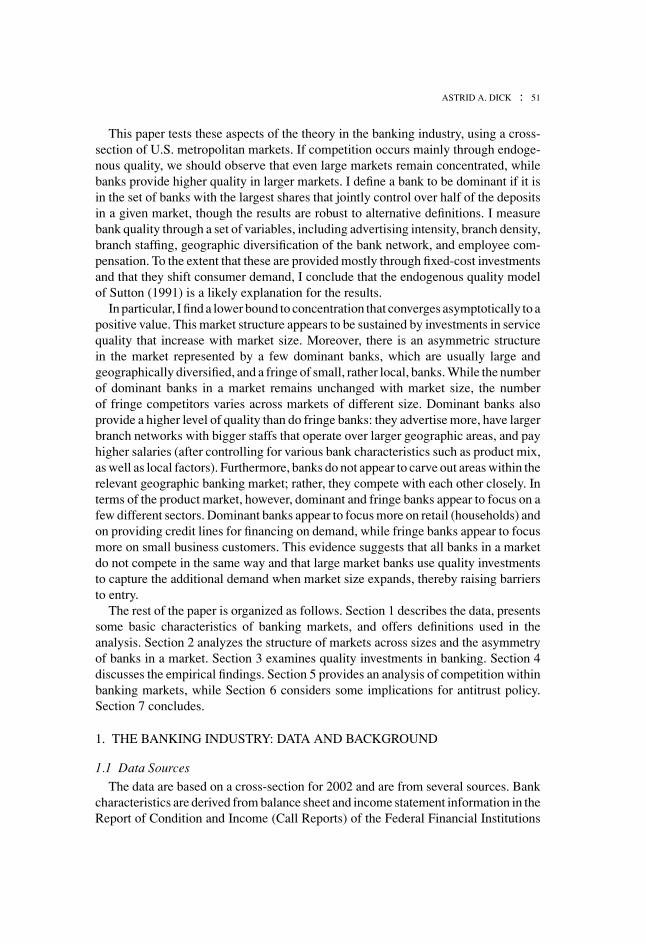
Market equilibrium. To draw generalizations from the current study, we would ide-ally like to analyze markets in equilibrium. The underlying assumption is that theindustry reached equilibrium in 2002, the year of the analysis. The assumption seemsreasonable given the tremendous shakeout the sector experienced throughout the lastthree decades and, in particular, in the 1990s, with the introduction of nationwidebranching throughout 1994–97.12 Figure 1 shows the number of bank mergers peryear for 1993–2003.13 There is an average of 393 mergers per year, and the number

9. This dominant/fringe bank definition appears to set an appropriate dividing line between banktypes. Taking the ranked distribution of market shares, the drop in market share from the last dominantbank to the next fringe bank is always bigger than (i) the drop between the last two dominant banks, and(ii) the drop between this fringe bank and the next—both in absolute and relative terms.

10. In particular, I define a dominant bank as one with the largest market share (or, alternatively, thosebanks with the largest two/three market shares). I also try defining dominance at 40% and 60%, insteadof the current 50% of market deposits. The results are robust (though not as strong sometimes), and thenumber of dominant banks is reduced/increased by around 25% (using the 40 and 60 “cuts,” respectively).

11. This is consistent with the empirical evidence. Dick (2006) finds that if a bank is dominant in theMSA of a given U.S. region (where a region covers several states), it is likely that it is also dominant inthe other MSAs within the region. Also, note that there is a lot of overlap in the identities of the dominantbanks across MSAs. For instance, out of a total of 4,091 banks in the sample, only 8% (346 banks) aredominant banks in a single MSA. The average number of markets in which these 346 banks are dominantis 2.5, with Bank of America at the top of the distribution with dominance in 94 of the 318 MSA marketsstudied in the paper.

12. Regulatory restrictions affecting the ability of banks to diversify geographically have decreaseddramatically. Deregulation of unit banking and limited branch banking occurred gradually throughout1970–94 in most states. Intrastate branching deregulation began in some states even before the 1970s,while interstate banking started as early as 1978. The process of deregulation of geographic expansionculminated in 1994 with the passage of the Riegle-Neal Interstate Banking and Branching Efficiency Act,which permitted nationwide branching as of June 1997.

13. The information in the figure is based on the author’s calculation using Banking Holding Companydata from the Federal Reserve Bank of Chicago.

ASTRID A. DICK : 55

FIG. 1. Bank Mergers per Annum (1993–2003)

each year decreases steadily since 1998. In addition, I find that the banks that havenegative (accounting) profits in 2002 and that would likely exit the market, tend to bepart of the fringe. Thus, the basic market structure between dominant and fringe banks,documented later in this paper, should not be affected by these industry developmentsin any significant manner.14

Compelling evidence is found in Dick’s (2006) analysis of branching deregulationduring 1993–99, where the structure of markets is shown to remain almost intactthroughout the period. In particular, she finds that MSA markets have between twoand three dominant banks across time, with no changes in concentration. In fact, onlyregional concentration increases (where a region covers several states and includesmany banking markets) following a reduction in the number of banks that have domi-nance over both a region and the markets within it. This suggests that market structureis persistent as time evolves, with variation only in the identities of the banks in themarket.

2. STRUCTURE OF BANKING MARKETS

2.1 Market Structure across Market Sizes

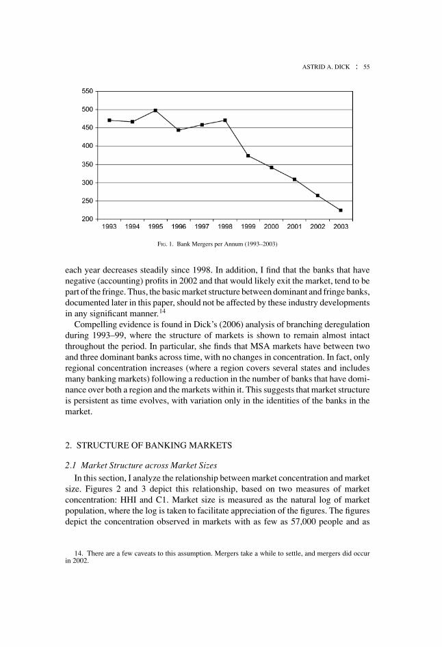
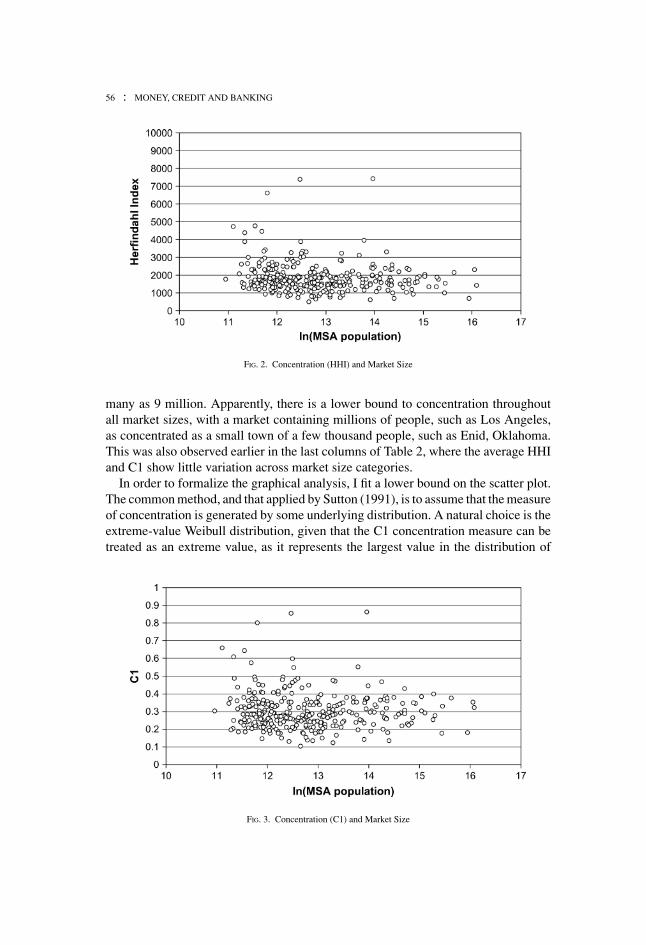
In this section, I analyze the relationship between market concentration and marketsize. Figures 2 and 3 depict this relationship, based on two measures of marketconcentration: HHI and C1. Market size is measured as the natural log of marketpopulation, where the log is taken to facilitate appreciation of the figures. The figuresdepict the concentration observed in markets with as few as 57,000 people and as

14. There are a few caveats to this assumption. Mergers take a while to settle, and mergers did occurin 2002.


FIG. 2. Concentration (HHI) and Market Size

many as 9 million. Apparently, there is a lower bound to concentration throughoutall market sizes, with a market containing millions of people, such as Los Angeles,as concentrated as a small town of a few thousand people, such as Enid, Oklahoma.This was also observed earlier in the last columns of Table 2, where the average HHIand C1 show little variation across market size categories.

In order to formalize the graphical analysis, I fit a lower bound on the scatter plot.The common method, and that applied by Sutton (1991), is to assume that the measureof concentration is generated by some underlying distribution. A natural choice is theextreme-value Weibull distribution, given that the C1 concentration measure can betreated as an extreme value, as it represents the largest value in the distribution of

FIG. 3. Concentration (C1) and Market Size

ASTRID A. DICK : 57

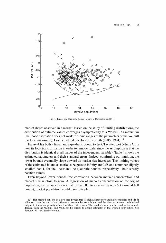
FIG. 4. Linear and Quadratic Lower Bounds to Concentration (C1)

market shares observed in a market. Based on the study of limiting distributions, thedistribution of extreme values converges asymptotically to a Weibull. As maximumlikelihood estimation does not work for some ranges of the parameters of the Weibull(no local maximum), I use a method developed by Smith (1985, 1994).15

Figure 4 fits both a linear and a quadratic bound to the C1 scatter plot (where C1 isnow its logit transformation in order to remove scale, since the assumption is that thedistribution is identical at all values of the independent variable). Table 4 shows theestimated parameters and their standard errors. Indeed, confirming our intuition, thelower bounds eventually slope upward as market size increases. The limiting valuesof the estimated bound as market size goes to infinity are 0.58 and a number slightlysmaller than 1, for the linear and the quadratic bounds, respectively—both strictlypositive values.

Even beyond lower bounds, the correlation between market concentration andmarket size is close to zero. A regression of market concentration on the log ofpopulation, for instance, shows that for the HHI to increase by only 5% (around 100points), market population would have to triple.

15. The method consists of a two-step procedure: (i) pick a shape for candidate schedules and (ii) fita line such that the sum of the difference between the lower bound and the observed values is minimizedsubject to the nonnegativity of each of these differences. The residuals can then be used as the samplederived from the Weibull, and MLE can be carried to obtain estimates of the Weibull distribution. SeeSutton (1991) for further details.


TABLE 4

LOWER BOUND ESTIMATION PARAMETERS

Linear QuadraticC1 = a + b/(lnS) C1 = a + b/(lnS) + c/(lnS)2

a 0.31 (0.68) 23.22 (3.96)∗∗b −31.22 (8.60)∗∗ −676.31 (102.82)∗∗c — 4494.80 (663.94)∗∗α 2.112 (0.090)∗∗ 1.585 (0.074)∗∗s 1.394 (0.039)∗∗ 1.190 (0.043)∗∗

C∞1 0.58 1.00†

NOTES: Standard errors in parentheses. C1 is the logit transformation of C 1. S is market size (population). α and s are Weibull parameters.C∞

1 is the limiting value of the distribution. †Approximation of 1 − ε, where ε is an extremely small number; ∗∗significant at 1%.

The fact that market concentration does not decrease as markets grow large is anextremely rich finding all in itself. For instance, it allows us to easily rule out variousmodels of bank competition, based on some very general characteristics and withouta formal model. First, we know that homogeneous goods industries will depict marketfragmentation as market size grows, regardless of the form of competition (whetherbanks are perfect competitors, at one extreme, or play a Cournot game, at the other).16

The number of banks sustainable by the market increases as setup costs decrease rela-tive to market size, and this phenomenon drives market concentration unambiguouslydownward. The above insight might not be very informative, however, since it iseasy to conclude through mere observation that homogeneous product competition isnot the appropriate model for banks (note, though, that much of the recent bankingliterature has rested implicitly and sometimes explicitly on this assumption).

Second, we also know that even some differentiated-goods industries will becomeless concentrated as market size increases. One example is that of single-product firmsthat are differentiated on a horizontal dimension (a la Hotelling), where products havedifferent attributes, as opposed to being better or worse. As market size grows, thisis like the spatial line (or circle, where banks are located) becoming longer, such thatmore firms can enter the market and take up the additional demand created by thelarger market.

Third, even in the case of quality competition or vertical differentiation, we canenvision situations in which the market structure fragments as market size grows. Thisoccurs in industries in which quality is provided mostly through variable costs. For in-stance, Berry and Waldfogel (2003) document this relationship for restaurants, which,albeit differentiated on quality, incur mostly greater variable costs in order to providebetter food (larger marginal costs), resulting in large markets being unconcentrated.

While we can rule out these competition models with a single finding, we are still leftwith several others that are consistent with it. The observed market structure couldarise under two main forms of competition: horizontal differentiation (no quality)with multiproduct firms, and vertical differentiation with quality provided mostly

16. Except monopoly, which does not interest us here.

ASTRID A. DICK : 59

TABLE 5

BANKING MARKETS BY POPULATION AND NUMBER OF DOMINANT BANKS

Number of dominant banks

Population 1 2 3 4 5 6 8 Total markets

<100K 2 8 5 1 0 0 0 16100K–200K 3 47 38 7 1 0 0 96200K–500K 3 32 45 13 6 2 1 102500K–1M 1 14 21 5 0 1 0 421M–2M 1 15 15 2 1 1 0 35>2M 0 14 10 2 0 1 0 27Total 10 130 134 30 8 5 1 318

In percentages†<100K 13% 50% 31% 6% 0% 0% 0% 100%100K–200K 3% 49% 40% 7% 1% 0% 0% 100%200K–500K 3% 31% 44% 13% 6% 2% 1% 100%500K–1M 2% 33% 50% 12% 0% 2% 0% 100%1M–2M 3% 43% 43% 6% 3% 3% 0% 100%>2M 0% 52% 37% 7% 0% 4% 0% 100%Total 3% 41% 42% 9% 3% 2% 0% 100%

NOTES: Year 2002. Dominant banks are defined as those that jointly control over half of the deposits in the market. †Out of total markets inthe given market size category.

through fixed costs, as described earlier. In the first case, markets might remainconcentrated because banks are able to develop several niche product markets asmarket size grows (product proliferation). Note that in the case of banking, however,the number of products is unlikely to be correlated with market size. In the secondcase, firms will invest in quality as market size grows, thereby raising barriers toentry. The following section will provide material to help discriminate between thesepossibilities.

FINDING 1: There exists a lower bound to concentration in banking markets, asmarket structure remains concentrated throughout all market sizes. Moreover, thecorrelation between market concentration and market size is close to zero.

2.2 Asymmetry and Number of Banks across Market Sizes

In this section, I explore further the industrial structure of banking markets byanalyzing asymmetry among firms.

Table 5 presents a tabulation of markets according to population and number ofdominant banks (for ease of interpretation, I also provide, in the lower panel, thenumber of markets in each cell as a percentage of the total markets in a given populationcategory).17 The table provides evidence of a striking fact: regardless of market size,the bulk of markets (83% of the MSAs) have either 2 or 3 dominant banks (with

17. Ellickson (Forthcoming) finds a similar structure for supermarkets.


FIG. 5. Deposit Share Lorenz Curve—Selected MSAs by Market Size Group

the rest of the markets having 1 to 8, with none in the 7 dominant bank category).Moreover, the correlation between the population and the number of dominant banksin a market is almost zero (0.03). This is interesting especially when contrasted withmodels in which fixed-cost quality does not play a role, such that the number of firmsgrows with market size as the number of consumers served per firm stays constant.

Deposit Lorenz curves18 provide another way to appreciate the fact that fewbanks control most of the market, regardless of the number of banks serving it andthe market size. Figure 5 shows several Lorenz curves for deposits, where banksare ranked on the x-axis according to their share of market deposits, while they-axis shows the cumulative share of deposits. Given the large number of MSAmarkets, for ease of analysis, the figure depicts only six markets, one for eachsize category19 (as defined in Table 2). The only apparent difference among themarkets is in the length of the tail of the curve, which grows in the number ofbanks serving the market. Below the 50% cumulative share line, markets differlittle

This description indicates that as markets grow, the number of dominant banksremains virtually unchanged. Naturally, as markets grow in population size, they alsotend to expand in the number of banks, yet this growth is only reflected in the length ofthe tail of the fringe and does not affect the dominant bank-fringe structure observedin smaller markets. Indeed, the number of banks in a market is highly correlated with

18. In a market with symmetric firms, the Lorenz curve would be a straight line, since all firms wouldhave the same market share. Thus, the closer the curves get to the y-axis, the more asymmetric, and thereforethe more concentrated, the market becomes.

19. The markets chosen are those that are most representative of the Lorenz curve structure withintheir population size category, both in terms of the number of firms and the market population. However,even if markets were chosen randomly, the figure would be similar. The markets shown in the figureare, in decreasing order of population size: Philadelphia, Pennsylvania; Fort Lauderdale, Florida; Vallejo-Fairfield-Napa, California; Hunstville, Alabama; Punta Gorda, Florida; and Pocatello, Idaho.

ASTRID A. DICK : 61

population size (0.77), yet the number of dominant banks is almost independent ofpopulation and the total number of banks in the market.

FINDING 2: Given a concentrated, asymmetric structure where dominant and fringebanks coexist, the number of dominant banks remains virtually unchanged with marketsize, with only the number of fringe banks increasing with market size.

3. QUALITY PROVISION IN BANKING

This section explores the provision of quality by banks in terms of the types ofcosts involved. To the extent that quality is offered by incurring mostly fixed costs,as opposed to variable costs, we should expect quality to increase with market size asbanks take up the additional demand and prevent entry by offering a higher qualityservice.

As far as the setup costs involved in opening a bank in the U.S. (“exogenous”fixed costs), the amount of capital needed averages around $7 million. However,there appears to be no legal minimum and there is great variation across states.A small portion of these setup costs are actually sunk costs, such as filing fees,branch construction costs, and legal fees.20 The process takes at least 7 months, and itincludes: (i) forming the organizing group (usually with a minimum of 5 individuals)that is capable of jointly holding at least a quarter of the bank’s capital; (ii) submittingan application to the corresponding regulatory authority (based on the type of charterchosen) with a filing fee of around $15,000; (iii) regulatory review; (iv) raising capital;and (v) regulatory approval.

The bank might also incur “endogenous” fixed costs if it chooses to invest inthings like advertising and certain types of quality. The key is that these investmentsshould involve mostly an increase in fixed outlays, as opposed to unit variable costs.In this section, I explore some of the most likely components of endogenous sunkcosts in banking. The data available do not allow for a complete and direct measureof these costs, but some observable bank characteristics provide an approximation.While some of the measures are far from perfect, the advantage is that many types ofinvestments are explored here.

3.1 Advertising and branding.

Advertising and developing a brand name are likely to be an important compo-nent of a bank’s endogenous sunk costs. According to surveys by the AmericanBankers Association, roughly 1% of bank operating costs, on average, was devotedto advertising in 1996, while total bank marketing expenditures were close to $4billion in 2001. Anecdotal evidence suggests that in the 1990s “[bank] marketinghas moved from a back room operation . . . to a front line strategic function.”21

20. Based on anecdotal evidence from Richardson (2003), “5 Phases of De Novo Formation,”Bankmark/Startabank (found in www.nubank.com). The amount of capital also depends on the type ofcharter and financial institution chosen, as well as the types of services the bank wants to provide.

21. “The Banks, They Are A’ Changin’,” D. Asher, Newspaper Association of America, 2003.


For instance, according to National Leading Advertising, BankAmerica Corp. wasthe 125th largest U.S. advertiser in 1996, with total expenditures of $145 million.Further evidence suggests that banks invest a growing fraction of their advertisingresources on branding campaigns and brand building, as well as on the developmentof in-house brand marketing departments and branding strategies.22 The importanceof branding in banking is also evident from the way in which merging banks choosetheir new brand name by keeping the bank name that customers are more familiarwith and/or is the strongest brand.23

Advertising outlays are likely to be correlated with the number of bank branches,based on anecdotal evidence on the greater role of the branch in the bank’s advertisingdecisions. Indeed, branches are a form of advertising for banks.24 There is plenty ofanecdotal evidence on how banks hope to attract customers using their branches, usu-ally with stylish merchandising and customer service.25 Banks become more visibleto consumers through their branches; in fact, banks are known to put clocks outsidetheir branches for this reason. Also, based on Radecki, Wenninger, and Orlow (1996),a typical branch has expenses of around $700,000 per year, and while the largestcomponent of this cost is staff compensation, advertising is usually part of it.

Given the scarcity of advertising data until recently, there is no academic work inthe area, with the exception of Ors (2003), who analyzes the role of advertising incommercial banking using new data for the period 2001–2002. Ors argues that adver-tising increases bank profitability and concludes that nonprice competition throughadvertising plays an important role in the industry.

Advertising expenditure data have become recently available for most banks in theCall Reports. In the analysis, I use advertising intensity, defined as marketing ex-penses normalized by assets.26 Only banks with advertising expenditure-to-operatingincome over 1% are required to report their advertising expenditures to the supervi-sory authorities. However, some banks report it even though they are not required todo so. In total, 56% of banks in the sample report their advertising expenses (with6% of them doing so voluntarily). Since the correlation between other noninterest

22. For instance, a search of “bank branding” on the American Banker magazine database finds thou-sands of articles, suggesting the prevalence of branding as a part of bank business.

23. A good example is the large NationsBank and BankAmerica merger in 1998: the BankAmericaname was chosen because of “its longer history” and “its patriotic feel which has more intrinsic appeal thanthe NationsBank name” (“Brand Name to Be Unveiled in Ads Tonight,” C. Guillam, American Banker,Sept. 30, 1998).

24. “With micromarketing, the promotional decisions are shifted from the corporate staff to the indi-vidual branches, where more is known about customers and prospects, such as where they live and whatthey buy. . . . There are less [sic] expensive television commercials and highly effective outdoor displays”(“It Pays to Think Small in Marketing,” K. Pelz, American Banker, March 4, 2002).

25. For example, some banks have tried installing coffee shops and “investment bars” within theirbranches (“Bank Branches Take a Page from Retail’s Book,” San Francisco Business Times, Sept. 2001).

26. I use advertising data at the banking holding company level, since much of the advertising by largemultibank holding companies gives name recognition to all banks in the holding (for example, televisionadds for JP Morgan Chase are not specific to the bank in a particular state). Moreover, banks might expensesome advertising at the banking holding company level. Thus, examining advertising at the bank level mayunderestimate the advertising of the largest banks. This, however, should be less of a concern for 2002,since by then most banking organizations had most of their assets in a single bank charter.

ASTRID A. DICK : 63

expenses—which include advertising and is reported by all banks in our sample—and advertising is close to 1, it is not difficult to impute the value for the fraction ofbanks that do not report the data. I do this using the coefficient from a regression ofadvertising intensity on noninterest expenses (also normalized by assets) based ona sample of reporting banks.27 Advertising should be a relatively clean measure ofquality, given that it is clearly unrelated to the number of customers of a bank: an adhas a given price regardless of how many people it reaches or how many get to seeit.

Branch and ATM networks. To the extent that banks open branches mostly in responseto their own market targets, as opposed to their existing customers’ needs, branchand ATM networks constitute another example of an endogenous fixed cost. Theanecdotal evidence indicates that banks open branches in the hope of shifting demandand thus attracting new customers. For instance, the CEO of Bank of America, one ofthe largest U.S. banks, has said that “customers especially want face-to-face contactwhen opening accounts and getting loans,” when explaining the bank’s ambitiousbranching strategy and the commitment to branch expansion industry-wide.28 A recentFDIC study on bank branch growth finds that this growth follows population andemployment growth, thus offering further evidence of the role of branches in shiftinga bank’s own demand (Spieker 2004). In a structural deposit demand study, Dick(2002) finds that branches play a major role in a consumer’s choice of bank.

At least some of the branch and ATM installation costs are clearly sunk (net ofany resale value).29 Once a facility is built, it is hard to recoup the incurred costs.As Radecki, Wenninger, and Orlow (1996) point out, the typical bank branch costsroughly $1 million to build. While a portion of this expense is for equipment, whichmay be removed and installed elsewhere,30 most of the cost covers construction.There is also anecdotal evidence suggesting that branches represent sunk costs. Forinstance, such evidence supported one of the main arguments for Internet banking(The European Internet Report, Morgan Stanley Dean Witter, June 1999).31

While the cost of opening a single branch might not be exactly fixed with respectto output, a bank’s overall branch density cost is likely to be largely independent ofoutput levels. In other words, branch networks are at least somewhat independent ofthe number of customers using them. While a consumer might do most of her bankingwith a single bank branch, she should still value the convenience of her bank’s overallnetwork. There is no question that the quality of an ATM card increases to the userwith the number of venues where the consumer can use it. Moreover, while in theory

27. The coefficient from this regression is 0.02 and it is significant at the 1% level of confidence.28. “Big Players Are Finding A Bottom in Branching,” American Banker, June 24, 2002.29. Some of the cost of branches could later be recouped if the bank is able to sell them in a merger or

acquisition.30. This is overly optimistic. In an era of rapid computer obsolescence, the salvage value of the

equipment is likely to be small. Also, the marketing research, the staff training costs, and the fraction ofemployees’ time involved in opening a new branch are clearly lost for good.

31. See also Sullivan (2001), based on a survey of banks and their website services.


there exists a maximum number of customers that a single branch can serve (or,for that matter, that a given employee or computer system memory can serve), itis unlikely to be binding in practice. This is suggested by the popularity in recentyears of the in-store or supermarket branch—a full-service branch located within alarge retail outlet—as a way to expand customer bases relative to a conventional bankbranch (Radecki, Wenninger, and Orlow 1996). Banks find these branches attractivenot only for cost-reduction purposes, but also because they provide access to largeflows of potential and existing customers (even though they have smaller staffs thantraditional branches): the typical supermarket averages 20,000–30,000 customers aweek, while the typical bank branch averages just 2,000–4,000 weekly customers(Williams 1997).

As a measure of a bank’s branch network in a market, I use branch density, defined asthe number of branches per square mile in a market. Data on ATMs are not available.However, the correlation between the number of ATMs and branches of a bank isactually 80%, based on a sample of almost 1,500 bank-market observations in 1998from Cirrus, the largest ATM network.32

As other measures of quality, I use the number of employees per branch; the geo-graphic diversification, measured as the number of states in which the bank operates;and salary per employee. The number of employees and a bank’s geographic di-versification have also been found to affect significantly the consumer’s choice ofdepository institution in Dick (2002), who uses a structural product-differentiateddemand model.

From the consumer’s perspective, more of each of these attributes is likely to bea good thing. Branch density and geographic diversification embody the size of theoverall bank network, and therefore the convenience to the consumer. The number ofemployees per branch captures some of the quality provided at the branch, since thelarger the branch staff, the shorter the waiting times and the greater the availabilityof valued human interaction.

Salary per employee is used here as an alternative measure of quality unrelated tobank size. In particular, salary paid to the bank’s employees should be correlated toquality, as more highly qualified employees, who can provide better service and ex-pertise, are more expensive. This is likely correlated with the degree of sophisticationof the products offered by the bank. Note, however, that salary could also be correlatedwith the degree of horizontal differentiation of a bank, as banks may choose to operatein different segments of the market, and therefore controlling for business focus mightbe important. Since one would expect wages to be higher in larger markets, salaryper employee is adjusted for local costs, using housing prices.

3.2 Sunk Costs across Market Sizes

I now turn to the relationship between quality and market size. Panel A of Table 6(Panel B is discussed in the next section) reports MSA-level regressions of quality

32. I thank Tim Hannan and Robin Prager of the Federal Reserve Board for kindly sharing the Cirrusdata.

ASTRID A. DICK : 65

TABLE 6

OLS REGRESSIONS OF QUALITY (BASE CASE)

Dependent variable

Advertising Branch Employees Number of Salary perintensity density per branch states employee

Explanatory variable (i) (ii) (iii) (iv) (v)

Panel ALn(population) 0.007 0.157 0.120 0.213 1.834

(0.002)∗∗ (0.037)∗∗ (0.014)∗∗ (0.031)∗∗ (0.323)∗∗Median income (’000) −0.000 0.013 0.002 −0.004 −0.052

(0.000)† (0.004)∗∗ (0.001) (0.003) (0.031)Observations 318 318 318 318 318R-squared 0.04 0.17 0.29 0.14 0.10Panel BDominant bank indicator 0.021 0.828 0.407 0.874 4.025

(0.008)∗∗ (0.039)∗∗ (0.035)∗∗ (0.196)∗∗ (0.582)∗∗MSA fixed effects YES YES YES YES YESObservations 6,670 6,669 6,717 6,798 6,670R-squared 0.10 0.47 0.17 0.20 0.17

NOTES: Year 2002. †significant at 10%; ∗significant at 5%; ∗∗significant at 1%. Standard errors are in parentheses. Advertising intensity (%)is defined in terms of assets. Branch density is number of branches per square mile, multiplied by 100. Employees per branch and number ofbranches are in logs. Salary per employee is in thousands. Panel A: Level of observation: MSA. The dependent variable is a deposit marketshare weighted average. Panel B: Level of observation: bank ∗ market. Standard errors are adjusted for within-bank dependence. Dominantfirms are defined as those who jointly control over half of the deposits in the market.

correlates on the log of population (controlling for median income), where quality ismeasured as the weighted average of the banks in the market (by deposit share).33

Quality is positively and significantly associated with market size for all measures,suggesting that banks provide higher quality, on average, in larger markets. Theresults imply, roughly, that for an increase in market population from the 25th tothe 75th percentile of the distribution, there is a 30% increase in branch density andgeographic coverage (the number of states in which the bank operates), a 14% increasein advertising intensity, and a 7% increase in branch staffing and in employee salary(adjusting for local prices).34

Presumably, much of the quality I measure here is driven by household demand,commonly referred to as retail; as a result, controlling for the degree of horizontaldifferentiation of the banks that make up the market could be important. Thus, Iintroduce a retail loan and a retail deposit ratio.35 Moreover, what we really want to

33. The results are even stronger if quality is added across banks or if the maximum quality in the marketis used. However, the weighted average is more appropriate here. Larger markets have more firms (due toa larger fringe set), so adding the quality will always bias the results toward finding an increase in qualitywith increases in market size. The idea behind using a weighted average is to capture the representativebank in the market.

34. Note that the results in this section are robust to clustering errors by region, since the error of MSAswithin a given region might not be independent.

35. I construct retail business as four-person family residential mortgages and loans to individuals,on the loan side, and small-time deposits and savings, on the deposit side (the measures are imperfect,however, given the data availability).


know is whether a given set of banks in a market provides more quality than another,otherwise similar, set of banks that operates in smaller markets. For instance, banks inlarger markets might be bigger, and bigger banks tend to engage more in non-depositbusiness such as off-balance sheet activities and lending to large firms. For this reason,I introduce further controls for bank size, fee income, and the characteristics of theloan and deposit portfolio. Bank size is constructed as deposits outside the market (inlogs) to diminish the high collinearity between assets and market size. The rest of thebank characteristics are constructed in terms of assets, except for the small businessand agricultural loans indicators, which take on a value of 0 or 1.

Lastly, since we might expect other market characteristics to influence the qualitychoice of a bank, I control for the level of education, age distribution, level of prices,and population density (population over MSA square miles). The latter is a particularlyrelevant control in the regression for branch staffing, since traveling in more crowdedareas might be slower and more costly and branches might also have longer lines.36

I also introduce the housing price index to account for local costs (except in the lastcolumn, since salary per employee has already been adjusted by this index).

Table 7 introduces in the earlier regressions these further market characteristics37

and a set of bank characteristics to capture the degree of retail business and otheractivities of banks in the market for both the loan and deposit portfolio. Note thatI use a one-year lag on these variables to avoid potential endogeneity, since qualityshould have an effect on demand for these services. The coefficients on market sizeremain positive and significant—though they decrease in magnitude—except for ad-vertising, where the coefficient is no longer significant (the coefficient is still positivebut decreases substantially). The coefficients remain economically significant as well(branch density increases by 23% with an increase in population from the 25th to the75th percentile, while geographic coverage increases by 13% and branch staffing andsalary per employee increase by 3%). The fit of the regression increases substantiallyin all cases, with more than half of the variation in branch staffing and geographiccoverage being explained by the regressors.

While our measures of quality are imperfect, similar results are obtained for all ofthem. This is a clear indication that unlike market structure, which does not vary muchacross markets, service characteristics differ significantly between large and smallmarkets. These results suggest that there is a role for endogenous quality competitionin banking.

FINDING 3: Quality increases with market size.

3.3 Sunk Costs across Banks

Having established a clear distinction among banks in terms of market presence, Inow explore whether dominant banks differ from other banks in terms of the servicequality they provide customers.

36. While market population and population density show a positive correlation (38%), the results arenot affected by including both in the regression (the results are only stronger when population density isremoved).

37. Demographic variables are known to be highly correlated. As a result, I have kept a few relevantvariables but corroborated that the results are robust to using a different set of demographic variables.

ASTRID A. DICK : 67

TABLE 7

OLS REGRESSIONS OF QUALITY AND MARKET SIZE

Dependent variable

Advertising Branch Employees Number Salary perintensity density per branch of states employee


Ln(population) 0.002 0.123 0.058 0.092 0.670(0.002) (0.039)∗∗ (0.014)∗∗ (0.023)∗∗ (0.349)†

Median income (’000) −0.000 0.013 0.000 −0.009 −0.086(0.000) (0.004)∗∗ (0.001) (0.002)∗∗ (0.035)∗

Pop. under 20 years (%) 0.002 −0.005 −0.002 −0.047 0.158(0.001)∗∗ (0.014) (0.005) (0.008)∗∗ (0.123)

High school grads (%) −0.001 0.041 −0.011 −0.031 0.021(0.000)† (0.009)∗∗ (0.003)∗∗ (0.005)∗∗ (0.082)

Population density 0.000 0.000 0.000 0.000 0.001(0.000) (0.000)∗∗ (0.000) (0.000) (0.000)∗∗

Housing price index 0.000 −0.001 0.002 −0.002(0.000)∗∗ (0.002) (0.001)∗ (0.001)†

Bank size 0.000 0.028 0.001 0.090 −0.001(0.001) (0.012)∗ (0.004) (0.007)∗∗ (0.107)

Retail loan ratio 0.001 0.009 0.003 −0.012 0.003(0.000)∗∗ (0.006) (0.002) (0.003)∗∗ (0.052)

Retail deposit ratio −0.001 0.008 −0.013 0.013 −0.051(0.000) (0.008) (0.003)∗∗ (0.005)∗∗ (0.071)

Real estate loans −0.115 0.170 −0.647 0.461 −8.256(0.024)∗∗ (0.479) (0.169)∗∗ (0.284) (4.332)†

Comm. & ind. loans 0.074 2.646 0.083 −0.571 −6.679(0.066) (1.298)∗ (0.459) (0.770) (11.766)

Leases 0.294 4.312 −0.333 10.764 16.69(0.167)† (3.270) (1.157) (1.941)∗∗ (29.621)

Commitment lines 0.003 −0.039 −0.036 0.154∗∗ 0.278(0.005) (0.097) (0.034) (0.058)∗∗ (0.883)

Mostly small −0.067 −1.349 −0.064 0.719 −2.820business loans (0.050) (0.986) (0.349) (0.586) (8.920)

Mostly small 0.009 −0.390 −0.415 −0.035 −12.784agricultural loans (0.019) (0.376) (0.133)∗∗ (0.223) (3.393)∗∗

Demand deposits 0.343 −0.593 −0.966 0.574 −12.116(0.075)∗∗ (1.460) (0.516) (0.867) (13.236)

Non-transaction deposits 0.018 0.220 −0.703 −1.003 −11.272(0.041) (0.803) (0.284)∗ (0.477)∗ (7.275)

Fee income 0.220 1.255 −0.988 −1.438 35.361(0.177) (3.458) (1.223) (2.053) (31.347)

Observations 318 318 318 318 318R-squared 0.31 0.40 0.52 0.69 0.29

NOTES: Year 2002. Level of observation: MSA; †significant at 10%; ∗significant at 5%; ∗∗significant at 1%. Standard errors are in parentheses.Advertising intensity (%) is defined in terms of assets. Branch density is number of branches per square mile, multiplied by 100. Employeesper branch and number of branches are in logs. Salary per employee is in thousands.

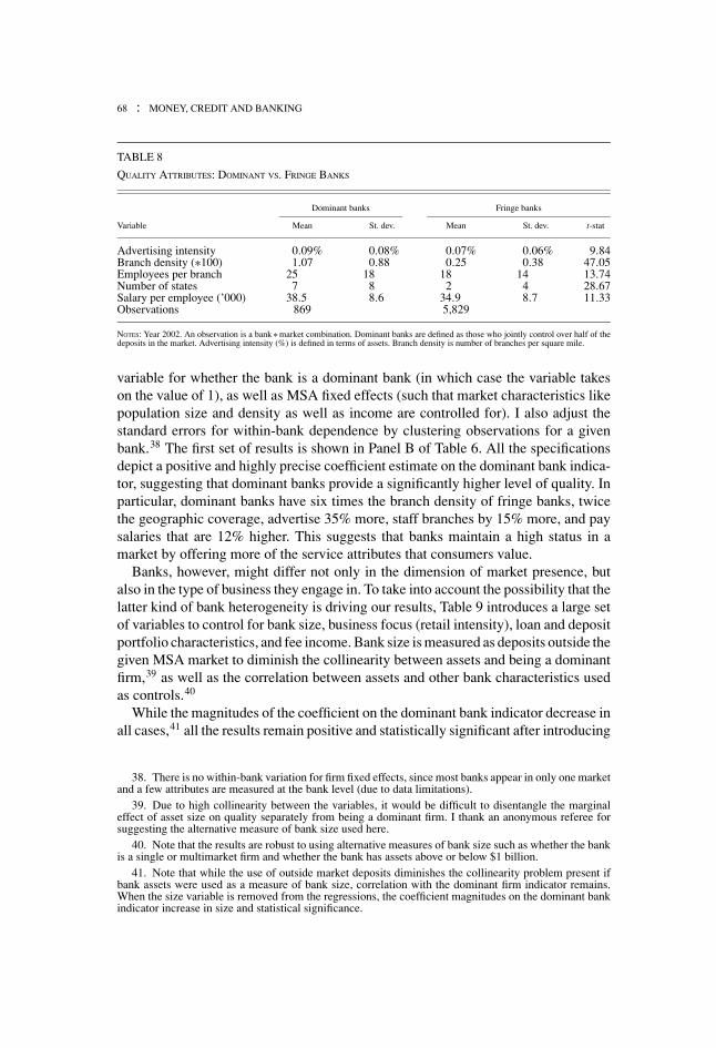
Table 8 shows means for various quality measures for dominant and fringe banks.The raw means, which are statistically different across bank types (as evidencedby the t-statistics in the last column), show that dominant banks do relatively moreadvertising and provide higher quality according to all of our measures. They havemore branches per square mile, more employees at the branch, a larger geographicpresence, and pay higher salaries.

I test for the significance of these quality differences by controlling for other fac-tors. In particular, I estimate quality of bank j in market m as a function of an indicator


TABLE 8

QUALITY ATTRIBUTES: DOMINANT VS. FRINGE BANKS

Dominant banks Fringe banks

Variable Mean St. dev. Mean St. dev. t-stat

Advertising intensity 0.09% 0.08% 0.07% 0.06% 9.84Branch density (∗100) 1.07 0.88 0.25 0.38 47.05Employees per branch 25 18 18 14 13.74Number of states 7 8 2 4 28.67Salary per employee (’000) 38.5 8.6 34.9 8.7 11.33Observations 869 5,829

NOTES: Year 2002. An observation is a bank ∗ market combination. Dominant banks are defined as those who jointly control over half of thedeposits in the market. Advertising intensity (%) is defined in terms of assets. Branch density is number of branches per square mile.

variable for whether the bank is a dominant bank (in which case the variable takeson the value of 1), as well as MSA fixed effects (such that market characteristics likepopulation size and density as well as income are controlled for). I also adjust thestandard errors for within-bank dependence by clustering observations for a givenbank.38 The first set of results is shown in Panel B of Table 6. All the specificationsdepict a positive and highly precise coefficient estimate on the dominant bank indica-tor, suggesting that dominant banks provide a significantly higher level of quality. Inparticular, dominant banks have six times the branch density of fringe banks, twicethe geographic coverage, advertise 35% more, staff branches by 15% more, and paysalaries that are 12% higher. This suggests that banks maintain a high status in amarket by offering more of the service attributes that consumers value.

Banks, however, might differ not only in the dimension of market presence, butalso in the type of business they engage in. To take into account the possibility that thelatter kind of bank heterogeneity is driving our results, Table 9 introduces a large setof variables to control for bank size, business focus (retail intensity), loan and depositportfolio characteristics, and fee income. Bank size is measured as deposits outside thegiven MSA market to diminish the collinearity between assets and being a dominantfirm,39 as well as the correlation between assets and other bank characteristics usedas controls.40

While the magnitudes of the coefficient on the dominant bank indicator decrease inall cases,41 all the results remain positive and statistically significant after introducing

38. There is no within-bank variation for firm fixed effects, since most banks appear in only one marketand a few attributes are measured at the bank level (due to data limitations).

39. Due to high collinearity between the variables, it would be difficult to disentangle the marginaleffect of asset size on quality separately from being a dominant firm. I thank an anonymous referee forsuggesting the alternative measure of bank size used here.

40. Note that the results are robust to using alternative measures of bank size such as whether the bankis a single or multimarket firm and whether the bank has assets above or below $1 billion.

41. Note that while the use of outside market deposits diminishes the collinearity problem present ifbank assets were used as a measure of bank size, correlation with the dominant firm indicator remains.When the size variable is removed from the regressions, the coefficient magnitudes on the dominant bankindicator increase in size and statistical significance.

ASTRID A. DICK : 69

TABLE 9

OLS REGRESSIONS OF QUALITY OF DOMINANT VS. FRINGE BANKS

Dependent variable



Dominant bank indicator 0.010 0.693 0.227 0.196 1.663(0.005)∗ (0.032)∗∗ (0.026)∗∗ (0.110)† (0.424)∗∗

Bank size 0.000 0.011 0.005 0.061 0.087(0.000) (0.001)∗∗ (0.002)∗ (0.008)∗∗ (0.043)∗

Retail loan ratio 0.038 0.035 0.151 0.144 −2.811(0.010)∗∗ (0.037) (0.077)∗ (0.123) (1.480)†

Retail deposit ratio 0.008 0.465 −0.543 0.293 −2.648(0.018) (0.055)∗∗ (0.162)∗∗ (0.255) (2.333)

Real estate loans −0.004 −0.120 0.182 −0.261 0.543(0.023) (0.044)∗∗ (0.123) (0.142)† (1.762)

Comm. & ind. loans 0.072 0.109 0.693 0.489 22.887(0.020)∗∗ (0.082) (0.180)∗∗ (0.246)∗ (3.403)∗∗

Leases 0.112 2.118 1.512 11.428 18.841(0.136) (0.435)∗∗ (0.898)† (2.946)∗∗ (15.756)

Commitment lines 0.004 −0.007 0.259 0.023 0.156(0.003) (0.007) (0.111)∗ (0.029) (0.301)

Mostly small −0.006 −0.019 −0.139 0.034 −0.423business loans (0.004)† (0.013) (0.029)∗∗ (0.039) (0.455)

Mostly small −0.008 0.028 −0.109 −0.039 −1.719agricultural loans (0.003)∗∗ (0.012)∗ (0.024)∗∗ (0.054) (0.480)∗∗

Demand deposits 0.035 0.045 −1.585 −0.670 −18.420(0.025) (0.090) (0.352)∗∗ (0.348)† (5.085)∗∗

Non-transaction deposits −0.010 −0.383 −0.721 −1.221 −10.063(0.027) (0.075)∗∗ (0.242)∗∗ (0.230)∗∗ (2.800)∗∗

Fee income 0.715 −0.780 3.083 0.791 40.502(0.141)∗∗ (0.262)∗∗ (1.178)∗∗ (1.331) (26.706)

MSA fixed effects YES YES YES YES YESObservations 6,670 6,669 6,717 6,798 6,670R-squared 0.19 0.52 0.33 0.62 0.29

NOTES: Year 2002. Adjusted for within-bank dependence standard errors are in parentheses; †significant at 10%; ∗significant at 5%;∗∗significant at 1%. A single observation is a bank ∗ market combination. Dominant banks are defined as those who jointly control over halfof the deposits in the market. Advertising intensity (%) is defined in terms of assets. Branch density is number of branches per square mile,multiplied by 100. Employees per branch and number of branches are in logs. Salary per employee is in thousands. Bank size is defined asdeposits outside the given MSA market, in logs.

the additional set of regressors. They also remain economically significant (dominantbanks have five times the branch density of fringe banks, 41% more geographiccoverage, 17% more advertising, 8% more branch staffing, and 5% higher salaries).This is strong evidence that dominant banks are indeed different and provide higherservice quality42—at least in terms of our measures—relative to fringe banks.43

42. Note that Bank of America, which is the top advertiser among banks in the U.S. (Financial ServicesAdvertising Report, American Banker, May 17, 2005), is also at the top of the distribution in terms of thenumber of times it is dominant in a market in our sample (94 out of 318 MSAs).

43. Dominant banks are different from fringe banks in other measures of quality as well. For instance,based on a survey of banks by the Federal Reserve, larger banks, which tend to be dominant in localmarkets (as will be seen in the next section), had much higher website adoption rates since the adventof the Internet, especially for websites with informational as well as transactional capabilities (Sullivan2001).


We established earlier that larger markets have higher quality than do smallermarkets. Coupled with the finding that dominant banks offer higher quality than dofringe banks, an implication of this might be that dominant banks in larger marketsoffer higher quality than do dominant banks in smaller markets. To explore thispossibility, I introduce a dummy variable for large MSAs and an interaction termbetween the dominant bank indicator and this large MSA indicator. The large MSAindicator takes the value of 1 if the MSA has a population greater than 1 million (over20% of the MSAs) and 0 otherwise. Since the regression now includes: (i) a dominantbank indicator, (ii) a large MSA indicator, and (iii) an interaction term between thetwo (plus controls and MSA fixed effects), the large MSA indicator captures whetherfringe banks in large MSAs provide levels of quality different from those of fringebanks in small MSAs (the base case is a fringe bank in a small MSA). Thus, thisregression allows us to explore the quality differences among dominant banks inlarge versus small markets, and the same for fringe banks.

The results, shown in Table 10, indicate that dominant banks in large MSAs providea significantly higher level of branch density and geographic coverage relative todominant banks in smaller markets. The rest of the coefficients on the interactionterm are also positive but not statistically significant (though advertising intensity issignificant at the 13% level). On the contrary, fringe banks show a lower level ofbranch density in larger MSAs relative to their counterparts in small markets, andmost of the other coefficients are negative (though not statistically significant).

This structure of two groups of banks might arise when some fraction of consumersare very sensitive to quality and the rest are less so or do not care at all. Then,the low-quality sector will tend toward fragmentation, as evidenced by the largernumber of fringe banks observed in larger markets—what certain models of horizontaldifferentiation predict should happen when market size grows. Thus, banking marketsappear to have a small number of leading banks that are high-quality providers,coexisting with a large fringe of lower quality banks that might focus on a differentset of consumers.

FINDING 4: Dominant banks provide higher quality than do fringe banks. Moreover,dominant banks in larger markets provide higher quality than do dominant banks insmaller markets.

4. DISCUSSION

The above findings suggest that competition among banks involves endogenoussunk costs. Banks appear to arrange themselves across a quality spectrum, with twotypes of firms emerging: the high-quality dominant banks and the lower quality fringebanks. The structure of the market appears to pivot on the competition among dom-inant banks that compete in quality. Since the number of fringe banks grows withmarket size, we might also infer that unlike dominant banks, competition amongfringe banks is not driven by the fixed-cost provision of quality.

ASTRID A. DICK : 71

TABLE 10

OLS REGRESSIONS OF DOMINANT AND FRINGE BANK QUALITY IN LARGE VS. SMALL MSAS

Dependent variable



Dominant bank indicator 0.008 0.553 0.218 0.140 1.630(0.004)† (0.028)∗∗ (0.024)∗∗ (0.083)† (0.451)∗∗

Large MSA −0.046 −0.568 0.260 −0.279 −1.83(0.033) (0.196)∗∗ (0.208) (0.274) (2.444)

Dominant bank ∗ 0.010 0.813 0.049 0.277 0.169Large MSA (0.007) (0.099)∗∗ (0.049) (0.133)∗ (0.969)

Bank size 0.000 0.010 0.005 0.061 0.0870.000 (0.001)∗∗ (0.002)∗ (0.008)∗∗ (0.043)∗

Retail loan ratio 0.038 0.021 0.150 0.137 −2.815(0.010)∗∗ (0.036) (0.077)† (0.120) (1.481)†

Retail deposit ratio 0.008 0.490 −0.542 0.302 −2.643(0.018) (0.055)∗∗ (0.162)∗∗ (0.251) (2.326)

Real estate loans −0.003 −0.082 0.184 −0.248 0.552(0.023) (0.043)† (0.122) (0.140) (1.755)

Comm. & ind. loans 0.072 0.098 0.691 0.482 22.883(0.020)∗∗ (0.079) (0.180)∗∗ (0.245)∗ (3.404)∗∗

Leases 0.110 2.053 1.507 11.391 18.822(0.136) (0.425)∗∗ (0.896)† (2.956)∗∗ (15.757)

Commitment lines 0.004 −0.005 0.258 0.023 0.156(0.003) (0.007) (0.111)∗ (0.029) (0.300)

Mostly small −0.006 −0.030 −0.139 0.029 −0.426business loans (0.004)† (0.013)∗ (0.029)∗∗ (0.039) (0.455)

Mostly small −0.008 0.025 −0.109 −0.041 −1.72agricultural loans (0.003)∗∗ (0.011)∗ (0.024)∗∗ (0.054) (0.480)∗∗

Demand deposits 0.036 0.120 −1.580 −0.637 −18.396(0.025) (0.093) (0.350)∗∗ (0.343)† (5.046)∗∗

Non-transaction deposits −0.009 −0.329 −0.717 −1.196 −10.046(0.027) (0.073)∗∗ (0.241)∗∗ (0.228)∗∗ (2.771)∗∗

Fee income 0.716 −0.726 3.089 0.819 40.507(0.141)∗∗ (0.261)∗∗ (1.176)∗∗ (1.329) (26.708)

MSA fixed effects YES YES YES YES YESObservations 6,670 6,669 6,717 6,798 6,670R-squared 0.19 0.56 0.33 0.63 0.29

NOTES: Year 2002. Adjusted for within-bank dependence standard errors are in parentheses; †significant at 10%; ∗significant at 5%;∗∗significant at 1%. A single observation is a bank ∗ market combination. Dominant banks are defined as those who jointly control over halfof the deposits in the market. A dominant bank in a large MSA is a dominant bank with presence in an MSA market with population greaterthan 1,000,000. Advertising intensity (%) is defined in terms of assets. Branch density is number of branches per square mile. Employees perbranch and number of branches are in logs. Salary per employee is in thousands. Branch density is multiplied by 100. Bank size is defined asdeposits outside the given MSA market, in logs.

Given the variation in quality investments across market sizes documented in thispaper, the results suggest that large branch networks act as an entry deterrent becauseentrants are not able to match the size and density of the networks of the incumbents.Incumbents are presumably able to spread over a larger customer base the additionalfixed-cost investments that a larger branch network entails, without necessarily chang-ing their prices. If this is indeed the case, we would expect incumbents to expand theirbranch networks in order to dominate a market, as opposed to several competitors


entering and branching extensively to mimic the quality of the incumbents. In thissense, the time of entry into the market might play a role.44

The results are congruous to those in a recent paper by Cohen and Mazzeo (2005),who find that banks in rural areas invest in denser branch networks when they facecompetition from multimarket banks, whereas they choose to have fewer brancheswhen the competition is made up of single-market banks or thrifts. An interest-ing piece of evidence is presented in Berger, Leusner, and Mingo (1997), who findthat banks have twice as many branches as would be required to minimize costs.Thus, the authors conclude that for this overbranching to be optimal, banks mustexpect to raise revenues as consumers value the extra convenience of a larger branchnetwork.

Other models, without endogenous quality, could explain the observed marketstructure, but none can explain the positive correlation between market size and prod-uct quality (such as homogeneous goods, horizontal differentiation). For instance, amodel of Bertrand competition, in which marginal costs are constant and asymmetricacross banks, could explain the fact that there is the same number of banks acrossmarket sizes, but not the escalation in quality investments we document here.45 Sim-ilarly, a model of scale economies could explain why large markets have such a smallnumber of dominant banks, but not why smaller markets do not appear to tend towardmonopoly.46 Even if antitrust regulation has influenced this outcome,47 there is stillno role for the escalation of quality in such a model, as economies of scale alonewould give rise to concentrated equilibria.48 Even taken descriptively, however, thefindings of this paper are rather striking and suggest strategic behavior in the bankingindustry. The straightforward fact that markets remain similarly concentrated acrossall market sizes, even taken in isolation, provides interesting insight into the waysbanks compete with each other.

44. Many dynamic stories are consistent with the market structure documented in this paper, as thereare several mechanisms that could lead a firm to become dominant in the market. The fact that dominantbanks tend to be older might suggest an early-mover advantage into local markets, sustained by customerswitching costs, as well as informational barriers, as in Dell’Ariccia, Friedman, and Marquez (1999).Berger and Dick (Forthcoming) find that the earlier a bank enters, the larger its market share is relative toother banks (controlling for firm, market, and time effects, as well as number of years in the market).

45. Moreover, the implicit assumption here of homogeneous goods is not a good one for banks, giventhe empirical evidence.

46. Yet there is no single MSA market with a single dominant firm, and both small and large marketsappear to have a similar number of dominant banks.

47. In particular, regulation that does not allow mergers that would result in a single bank having overhalf of the market’s deposits. Given this paper’s definition of “dominant,” a lower bound on the HHI insuch a market would be 2,500, above the Department of Justice Antritrust Division’s high concentrationthreshold of 1,800.

48. In terms of the evidence on economies of scale in banking, extensive empirical work in the fieldsuggests that they exist for small-sized banks, while scale diseconomies are experienced by banks of largersize (see Berger and Mester 1997 for a survey of this literature). In addition, while some bank productsmight show increasing returns to scale in production (for example, electronic payment processes), thereappear to be decreasing returns to scale in management as banks grow into larger organizations. However,Hughes et al. (2000) argue that standard techniques to estimate scale economies do not appropriatelyaccount for the interplay between bank capital, risk, and managerial preferences in the production functionof the bank, and, as a result, they find scale economies are much larger once the adjustment is made.

ASTRID A. DICK : 73

While a dynamic and historical analysis of the banking industry is outside the scopeof this paper, it is useful to point out certain features of the industry’s development.The dual market structure of leading banks that advertise heavily along with a localfringe of non-advertisers (or advertisers on a much smaller scale) has existed fora long time, but the profile of the banks in each group has changed over time—inparticular, in the group of advertisers. In the latter group, big-market banks havehistorically advertised and enjoyed a brand image, but in the last decade they haveusually increased their geographic diversification dramatically, sometimes going fromregional or even local banks that just happened to enter first to national brand nameslike Bank of America (usually through a merger by buying one of the largest marketbanks). In the dynamism that the industry experienced throughout the 1980s, andespecially the 1990s with the 1994 passage of the Riegle-Neal Act, which allowednationwide branching, the fact that the big brand names became the leaders acrosslocal banking markets is consistent with the framework provided in this paper.

5. COMPETITION ANALYSIS: CARVING OUT “NEIGHBORHOODS” ANDPRODUCT MARKETS

The previous sections established that banking markets remain concentrated re-gardless of market size and that roughly the same number of dominant banks serveeach market, as predicted by a model in which banks compete on fixed-cost qualityinvestments. This structure, however, is consistent with various models of “localized”competition. One might ask, for instance, whether banks are able to carve out geo-graphic areas (“neighborhoods”) or product markets within the relevant geographicmarket. Using much of the insight provided by Ellickson (Forthcoming) in his studyof market segmentation for supermarkets, I now examine: (i) whether dominant bankscontrol geographic areas or instead compete head-to-head within a given MSA, (ii)whether dominant and fringe banks serve different geographic areas within the MSA,and (iii) whether dominant and fringe banks carve out different product markets.

5.1 Do Dominant Banks Control Geographic Areas or Compete Head-to-Headwithin a Given MSA?

While the bulk of the evidence suggests that the relevant geographic market is atthe MSA level, one might ask whether dominant banks either segment the marketor compete head-to-head within a given MSA (at a minimum, this is useful as asensitivity analysis of the results on market structure to the particular relevant marketdefinition). For instance, suppose that in a given market, dominant bank A has tenbranches. Then, another dominant bank B in that market, with ten branches as well,could have each one of them located near bank As branches, or alternatively, locatedin very different “neighborhoods” of the MSA.

To explore this, I break each MSA down into cities (or towns) and counties. Thereare 8,563 cities and 842 counties for the 318 MSAs present in the sample. Cities are


rather small sections within the MSA, with an average of 27 per MSA.49 Countiesare much larger areas, comprising several cities and towns. An average MSA hasbetween two and three counties. At this point, it is worth noting that any referencein this analysis to dominant or fringe banks is based on the earlier definitions, at thelevel of the MSA.

Breaking MSA markets down into cities and counties suggests that dominant banksdo not carve out geographic market niches within the MSA.50 First, counties servedby only one bank are few; moreover, they are controlled mostly by fringe banks.In particular, only 5 out of a total of 842 counties actually have a single bank, andnone of these 5 counties are controlled by a dominant bank. Cities with a single bankrepresent 42% of all cities, and only one-third of these cities has a dominant bankas the monopolist. Note, however, that the area covered by these cities appears to bevery small: over 90% of the monopoly cities have only one branch. Thus, an area witha single branch can hardly be a carved-out market “niche.”

Second, if there is one dominant bank in a given area, it is likely that there isanother dominant bank. In particular, outside the monopoly areas described above,the number of dominant banks is above one in most cities and counties. The number ofdominant banks usually ranges from two to three in both cities and counties. Moreover,conditional on there being two or more banks in the area, about half of cities and only10% of counties have a single dominant bank. This fact is relevant if one believesthat competition from another dominant bank is important in curtailing the marketpower of an incumbent dominant bank. These findings suggest that at various levelsof disaggregation within the MSA, dominant banks do not appear to hold distinctgeographic areas, and instead seem to compete head-to-head.

5.2 Do Dominant and Fringe Banks Serve Different Geographic Areas withina Given MSA?

An alternative possibility to market segmentation is that dominant and fringe banksserve distinct geographic areas within the MSA. This possibility is easily ruled outby the data.

First, most areas have dominant banks overlapping with fringe banks. Monopolyareas, as mentioned earlier, are rare. Areas with multiple banks but with only onebank type represent a small portion (13% of cities and 7% of counties) and are mostlyserved by fringe banks. Moreover, these areas tend to be geographically small, withtwo to three banks serving them and one or two branches per bank.

49. In the Boston MSA, for instance, some cities and towns include Boston, East Boston, Braintree,Brookline, Cambridge, Belmont, Chelsea, and Newton.

50. Note that I also calculated the market shares at the county level for dominant firms and found thatthe distribution of shares is very similar to that observed at the MSA level. In particular, whenever thereis geographic overlap in counties between dominant firms (most cases, as shown), their market shares arealso similar: among dominant firms, the largest share is 0.28 while the second largest share is 0.17 (medianand mean). Thus, a situation in which two banks are located in the same two counties but market sharesare split at a very high and a very low level in one and the reverse in the other county does not seem tohold. This makes sense since such would hardly be an enforceable equilibrium, given that both banks arecompeting for the same customers and geographically close.

ASTRID A. DICK : 75

FIG. 6. Dominant versus Fringe Branch Locations in Philadelphia MSA

Second, dominant and fringe banks tend to locate their branches near each other.Figure 6 shows the location of each branch throughout the Philadelphia MSAmarket,51 which is fairly representative of other MSA markets in this respect. Thecircles in the figure represent branches belonging to Philadelphia’s dominant banks,while the triangles depict branches of the fringe. The amount of overlap betweenthese two types of banks over the MSA is striking: most circles in the figure have atriangle next to it.

The evidence indicates that even at the level of analysis of such a small unit as acity, dominant banks do not appear to be segmenting the market away from fringebanks, but tend to serve the same geographic areas. Indeed, the dominant/fringe bankstructure documented at the level of the MSA appears to be relevant even withinsmaller geographic areas within it.

5.3 Do Dominant and Fringe Banks Carve out Different Product Markets?

This section explores whether dominant banks serve different customers from thoseof fringe banks, as well as other characteristics. While the analysis is mostly descrip-tive, it is another way of exploring the dual bank structure found earlier. The anal-ysis focuses on several balance sheet and income statement items for both types ofinstitutions, in order to gain insight into their asset and liability portfolio, productmix, and performance.

51. Note that most, but not all, of the branches in the Philadelphia MSA are shown on the map. Themapping software was able to match up to 73% of the branch addresses in our data.


First, note that dominant banks are significantly larger than fringe banks.52 Themedian asset size is $25 billion, versus $249 million for the median fringe bank. Interms of bank products, one significant difference between dominant and fringe banksis in the proportion of assets allocated to commitment or credit lines (an off-balancesheet item): while dominant banks allocate close to 40% of their assets to commitmentlines, fringe banks dedicate about half of this. The central feature of a commitmentis that a borrower has the option to take the loan on demand over some specifiedperiod of time, thus representing great value to a bank’s client. Given the nature of acommitment, this might be suggestive of a difference in service quality between thetwo bank types (emphasizing earlier findings in this paper), as opposed to a distinctproduct market niche.

Another marked difference between dominant and fringe banks is in the proportionof small loans (defined as less than $100,000 in the FFIEC form reported by banks tothe regulatory agencies). While 8% of business loans and 17% of agricultural loansare small in the case of fringe banks, the proportion of these loans is significantlysmaller in the case of dominant banks (0.3% and 5%, respectively). Although thiscould simply be driven by the regulatory restrictions on the loan size that smallerbanks can offer, there is, in fact, an extensive literature that documents the focus ofsmaller banks on lending to small firms, known as “relationship” lending (Berger et al.2005, Cole, Goldberg, and White 2004). On the liability side, dominant banks appearto have lower ratios of demand, non-transaction, and time deposits over $100,000,which might be reflective of their different funding structures.

In terms of retail business (households, as defined here), dominant banks depict alarger share on both the loan and deposit sides (42% and 64%, respectively, against38% and 59% for fringe banks). This is consistent with the branching strategiesof dominant banks, which, as we saw earlier, have much larger branch networkscompared with fringe banks—to the extent that branches are provided primarily toserve the retail sector. Indeed, in the earlier bank-level regression analysis, the shareof retail deposits is positively associated with branch density.

In terms of prices,53 the differences are usually small, though they are all statis-tically significant. Dominant banks do charge slightly higher interest rates on loansto individuals (mostly credit card loans), charge higher fees on checking accounts,and pay lower interest rates on deposits. This could be related to quality differencesbetween the two types of banks, documented earlier.

Dominant banks appear to perform much better than fringe banks in terms of ac-counting profits. While fringe banks enjoy a return on equity of 11%, with a largestandard deviation of 9 percentage points, dominant banks’ profits are more concen-trated around 15%. In fact, while the number of dominant banks losing money isnegligible, many of the fringe banks (over 8%) are making negative profits, whichexplains the higher turnover in fringe banks. Dominant banks, however, might bechoosing a higher level of risk, as their credit portfolio has a slightly higher level

52. This difference, as well as the other differences between dominant and fringe banks described inthis section, is statistically significant.

53. Prices are imputed using the income/expense flows from the income statement, adjusted by thecorresponding balance sheet stocks.

ASTRID A. DICK : 77

of charge-off losses in terms of assets (0.9% versus 0.5% of the fringe)—though inlight of their profitability, these are likely to be priced appropriately. They also showslightly lower operating costs (3.1% versus 3.3%) and a higher reliance on noninterestincome (2.0% versus 1.4%), both in terms of assets.

The descriptive analysis suggests that dominant banks focus more on retail business,as well as offering financing on demand. Fringe banks appear to focus more on servingsmaller businesses. It is difficult, however, to interpret the results on prices, costs, andprofits, given that only one year is analyzed and the overall nature of the analysis.

FINDING 5: Banks do not carve out areas within the relevant geographic bankingmarket, but rather compete with each other closely. However, in terms of the productmarket, dominant and fringe banks might focus on a few different sectors.

6. IMPLICATIONS FOR ANTITRUST POLICY

The regularities in market structure across markets found above do not appearto be unique to the specific year of our analysis, but seem to persist over time. Asmentioned earlier, Dick (2006) finds that the structure of markets remained almostintact throughout 1993–99 during the implementation of nationwide branching. Thus,the implications that follow from the analysis in terms of antitrust regulation and theimpact of industry consolidation could be significant.

Even beyond the Sutton (1991) model, the introduction of quality investment inthe study of competition alters the interpretation of certain empirical correlationsbetween the number of firms, market concentration, and prices used in antitrust policy.In particular, the finding that markets with fewer banks tend to have lower depositrates and higher loan rates (Rhoades 1996, Amel 1997) has historically been taken toimply a less competitive conduct by banks and therefore a bad thing for consumers.Also, Hannan and Prager (2004) find higher bank prices (lower deposit rates) inlarger markets, while Hannan (2001, 2002) finds that large banks charge higher fees,on average, than do small banks. Note that while an increase in prices following anincrease in quality is not a prediction of the Sutton model (since quality is assumedto be provided mostly through sunk cost investments that do not affect price-costmargins), the findings of this paper suggest that bank quality plays an important roleand therefore needs to be incorporated into the analysis of consumer welfare. Whileit is not clear from the literature whether prices are higher due to higher fixed-costquality, variable-cost quality characteristics, or other factors affecting larger marketsand larger firms, if consumers are receiving higher quality and are benefiting as aresult, they are not necessarily hurt by the higher prices they have to pay for them.Thus, once quality is controlled for, there is no unambiguous implication one canmake about consumer welfare from the empirical correlation between prices and thenumber of banks in a market. This paper documents not only a role for quality in bankcompetition, but also the existence of a dual industry structure in which, if anything,the total number of banks in each segment might be a more informative statistic thanthe total number of banks in the market.


Both the Department of Justice and the Federal Reserve Board54 focus on marketconcentration to determine whether a contemplated merger might cause anticompeti-tive concerns (see Amel 1997). In particular, their criteria include whether a proposedmerger would result in a market HHI greater than 1,800 and increase it by more than200 points (the “1,800/200 rule”) and whether the market share of the post-mergerbank would be 35% or more of deposits. In light of the current findings, a relevantquestion might be whether the new bank would provide a higher level of quality. Forexample, will the merger increase the ATM network available to consumers? If thepost-merger bank becomes dominant, will it have competition from other dominantbanks? Will the new bank be one of the big advertisers in the market (which canprovide insight into other areas)? Will it be a regional bank with a large network overseveral nearby states and is this feature one that the consumers in the market are likelyto value? The use of marginal utility estimates on both price and nonprice attributes(such as those provided in Dick 2002) can provide an estimate of the consumer surpluseffects associated with the likely changes in quality and pricing after the merger.

Lastly, whenever a proposed merger violates the above-mentioned screen, regula-tors consider what are supposed to be mitigating factors for the potential anticom-petitive effects of the merger. These include the case of an unusually large numberof competitors, based on the presumption that the number of banks in a market has apositive effect on competition, as well as the case of a recent trend toward deconcen-tration in the market where the merger is to take place. Yet in light of the analysis inthis paper, it should matter whether the new bank becomes a dominant bank, as thecompetition effects from other dominant banks should be quite different from those offringe banks. In addition, a trend toward deconcentration in a market could simply bethe result of fringe bank entry, which should not affect significantly the competitiveenvironment of a market.

7. CONCLUDING REMARKS

This paper’s findings, taken by themselves, constitute a set of novel and strikingstylized facts and results that can be useful in future theoretical and empirical workon the banking industry. Coupled with the insight of Sutton’s (1991) work, they alsoprovide a nuanced picture of how banks compete and what is behind the observedstructure in banking markets.

This paper might also contribute to the empirical literature on the relationshipsbetween market concentration, market size, and quality. While the theory of marketstructure and quality offers a set of robust predictions, the body of empirical work doc-umenting them is small. While this study focuses on the banking industry, Ellickson(Forthcoming) and Berry and Waldfogel (2003) obtain similar findings for supermar-kets and newspapers, respectively, suggesting that much of retail competition may be

54. The Federal Deposit Insurance Corporation and the Office of the Comptroller of the Currency alsohave regulatory authority, but they have not been very active in antitrust enforcement in recent years.

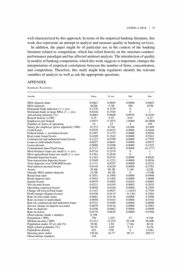
ASTRID A. DICK : 79

well characterized by this approach. In terms of the empirical banking literature, thiswork also represents an attempt to analyze and measure quality in banking services.

In addition, the paper might be of particular use in the context of the bankingliterature related to competition, which has relied heavily on the structure-conduct-performance paradigm and has affected antitrust analysis. The introduction of qualityin models of banking competition, which this work suggests is important, changes theinterpretation of empirical correlations between the number of firms, concentration,and competition. Therefore, this study might help regulators identify the relevantvariables of analysis as well as ask the appropriate questions.

APPENDIX

SUMMARY STATISTICS

Variable Mean St. dev. Min Max

MSA deposit share 0.0467 0.0805 0.0000 0.8603MSA deposits 442M 2.3B 2M 107BDominant bank indicator (1 = yes) 0.1278 0.3339 0 1Dominant bank in large MSA (1 = yes) 0.0246 0.1548 0 1Advertising intensity (%) 0.0684 0.0608 0.0070 0.4249Branch density (∗100) 0.35 0.55 0.01 4.23Employees per branch 2.9937 5.1075 1.0000 26.0000Number of states of operation 19 15 4 199Salary per employee (price adjusted) (’000) 35.372 8.748 18.088 83.609Cash/Assets 0.0529 0.0432 0.0006 0.6448Federal funds + securities/Assets 0.2497 0.1375 0.0000 0.9858Real estate loans/Assets 0.4189 0.1542 0.0000 0.9241Commercial and industrial loans/Assets 0.1223 0.0790 0.0000 0.7595Loans to individuals/Assets 0.0627 0.0681 0.0000 0.9675Leases/Assets 0.0088 0.0208 0.0000 0.4103Commitment lines/Total loans 0.2117 0.6674 0.0000 43.2771Most business loans are small (1 = yes) 0.0716 0.2579 0 1Most agricultural loans are small (1 = yes) 0.1561 0.3630 0 1Demand deposits/Assets 0.1162 0.0743 0.0000 0.8826Non-transaction deposits/Assets 0.5949 0.1233 0.0000 0.9036Time deposits over $100,000/Assets 0.1171 0.0797 0.0000 0.8252Non-interest income/Assets 0.0145 0.0229 0.0000 0.3782Assets 29.8B 99.3B 3.1M 622BOutside MSA market deposits 14.5B 50.1B 0 >310BRetail loan ratio 0.3851 0.1905 0.0000 0.9998Retail deposit ratio 0.5942 0.1402 0.0000 1.0000Equity/Assets 0.0979 0.0405 0.0265 0.8003Net income/Assets 0.0331 0.0195 0.0003 0.3835Operating expenses/Assets 0.0058 0.0104 0.0000 0.2305Charge-off losses/Total loans 0.1147 0.0927 −1.0453 0.7769Profit margin (Equity/Assets) 0.0106 0.0115 −0.1361 0.2284Rate on real estate loans 0.0661 0.0136 0.0008 0.1898Rate on loans to individuals 0.0058 0.0163 0.0000 0.5102Rate on commercial and industrial loans 0.0721 0.0289 0.0000 0.6000Service charge on deposit accounts 0.0070 0.0116 0.0000 0.2982Rate on deposits 0.0196 0.0062 0.0000 0.0909Rate on leases 0.0776 0.0625 0.0000 0.9768Observations (bank ∗ market) 6,798Population (’000) 730 1,225 57 9,768Median income (’000) 53.411 11.015 29.100 96.000Population under 20 yrs old (%) 28.06 2.84 17.66 40.26High school graduates (%) 18.70 4.69 8.13 34.58Population density 422 938 6 13,061Housing price index 139.66 16.77 99.13 209.33Observations (market) 318


DESCRIPTION OF VARIABLES

Variable Description

Dominant bank indicator (1 = yes) Bank is in set of banks with largest shares that jointly holdover half of the market’s deposits

Dominant bank in large MSA (1 = yes) Bank is dominant bank in MSA with population over 1MAdvertising intensity Marketing expenses/AssetsBranch density Number of branches in local market/Square miles of local

marketEmployees per branch Number of bank employees/Number of branchesNumber of states Number of states in which the bank has branchesSalary per employee (price adjusted) Salary expense/Number of employees, adjusted by the

Housing Price IndexMost business loans are small (1 = yes) If all or substantially all of the dollar volume of loans

secured by nonfarm nonresidential properties andcommercial and industrial loans have amounts of$100,000 or less

Most agricultural loans are small (1 = yes) If all or substantially all of the dollar volume of loanssecured by nonfarm farmland and loans to financeagricultural production and other loans to farmers haveamounts of $100,000 or less

Retail loan ratio Real estate loans secured by 1–4 family residentialproperties + Loans to individuals, over Loans

Retail deposit ratio Savings deposits + Time deposits of less than $100,000,over Deposits

LITERATURE CITED

Adams, Robert M., Kenneth Brevoort, and Elizabeth K. Kiser. (Forthcoming) “Who Competeswith Whom? The Case of Depository Institutions.” Journal of Industrial Economics.

Amel, Dean F. (1997) “Antitrust Policy in Banking: Current and Future Prospects.” Proceedingsof the 33th Annual Conference on Bank Structure and Competition, Federal Reserve Bankof Chicago.

Berger, Allen N., and Astrid A. Dick. (Forthcoming) “Entry into Banking Markets and theEarly-Mover Advantage.” Journal of Money, Credit, and Banking.

Berger, Allen N., John H. Leusner, and John J. Mingo. (1997) “The Efficiency of BankBranches.” Journal of Monetary Economics, 40, 141–62.

Berger, Allen N., and Loretta J. Mester. (1997) “Inside the Black Box: What Explains Dif-ferences in the Efficiencies of Financial Institutions.” Journal of Banking and Finance, 21,895–947.

Berger, Allen N., Nathan H. Miller, Mitchell A. Petersen, Raghuram G. Rajan, and JeremyC. Stein. (2005) “Does Function Follow Organizational Form? Evidence from the LendingPractices of Large and Small Banks.” Journal of Financial Economics, 76, 237–69.

Berry, Steven, and Joel Waldfogel. (2003) “Product Quality and Market Size.” NBER WorkingPaper No. 9675.

Cohen, Andrew, and Michael Mazzeo. (2005) “Investment Strategies and Market Structure:An Empirical Analysis of Bank Branching Decisions.” Working paper.

Cole, Rebel A., Lawrence G. Goldberg, and Lawrence J. White. (2004) “Cookie-cutter versusCharacter: The Micro Structure of Small Business Lending by Large and Small Banks.”Journal of Financial and Quantitative Analysis, 39, 227–51.

ASTRID A. DICK : 81

Dell’Ariccia, Giovanni, Ezra Friedman, and Robert Marquez. (1999) “Adverse Selection as aBarrier to Entry in the Banking Industry.” Rand Journal of Economics, 30, 515–34.

Dick, Astrid A. (2002) “Demand Estimation and Consumer Welfare in the Banking Industry.”Finance and Economics Discussion Series, Federal Reserve Board, 2002–58.

Dick, Astrid A. (2006) “Nationwide Branching and Its Impact on Market Structure, Qualityand Bank Performance.” Journal of Business, 79, 567–92.

Ellickson, Paul B. (Forthcoming) “Does Sutton Apply to Supermarkets?” Rand Journal ofEconomics.

Hannan, Timothy H. (2001) “Retail Fees of Depository Institutions, 1994–99.” Federal ReserveBulletin, 1–11.

Hannan, Timothy H. (2002) “Retail Fees of Depository Institutions, 1997–2001.” FederalReserve Bulletin, 405–13.

Hannan, Timothy, and Robin Prager. (2004) “The Competitive Implications of MultimarketBank Branching.” Journal of Banking and Finance, 28, 1889–1914.

Hughes, Joseph P., William Lang, Loretta J. Mester, and Choon-Geol Moon. (2000) “Recov-ering Risky Technologies Using the Almost Ideal Demand System: An Application to U.S.Banking.” Journal of Financial Services Research, 18, 5–27.

Ors, Evren. (2003) “The Role of Advertising in Commercial Banking.” Proceedings of the 39thAnnual Conference on Bank Structure and Competition, Federal Reserve Bank of Chicago,454–70.

Radecki, Lawrence J., John Wenninger, and Daniel K. Orlow. (1996) “Bank Branches inSupermarkets.” Current Issues in Economics and Finance, Federal Reserve Bank of NewYork, 2.

Rhoades, Stephen A. (1996) “Competition and Bank Mergers: Directions for Analysis fromAvailable Evidence.” The Antitrust Bulletin, 41, 339–64.

Shaked, Avner, and John Sutton. (1983) “Natural Oligopolies.” Econometrica, 51, 1469–84.

Shaked, Avner, and John Sutton. (1987) “Product Differentiation and Industrial Structure.”Journal of Industrial Economics, 36, 131–46.

Smith, Richard L. (1985) “Maximum Likelihood Estimation in a Class of Nonregular Cases.”Biometrika, 72, 67–90.

Smith, Richard L. (1994) “Nonregular Regression.” Biometrika, 81, 173–83.

Spieker, Ronald. (2004) “Bank Branch Growth Has Been Steady—Will It Continue?” FDICFuture of Banking Study.

Sullivan, Richard J. (2001) “Performance and Operation of Commercial Bank Web Sites.”Financial Industry Perspectives, Federal Reserve Bank of Kansas City, 23–33.

Sutton, John. (1991). Sunk Cost and Market Structure: Price Competition, Advertising, andthe Evolution of Concentration. Cambridge: MIT Press.

Williams, Christopher A. (1997) “Banks Go Shopping for Customers.” The RegionalEconomist, Federal Reserve Bank of St. Louis, October, 12–13.

Documents

Market Size, Service Quality, and Competition in Bankingfaculty.insead.edu/dick/personal/documents/Marketsize... · · 2009-06-26Market Size, Service Quality, and Competition in