Discussion Paper No. 820

MARKET SIZE AND

VERTICAL STRUCTURE IN THE RAILWAY INDUSTRY

Noriaki Matsushima Fumitoshi Mizutani

October 2011

The Institute of Social and Economic Research Osaka University

6-1 Mihogaoka, Ibaraki, Osaka 567-0047, Japan

Market Size and Vertical Structure in the Railway Industry∗

Noriaki Matsushima†

Institute of Social and Economic Research, Osaka University

Fumitoshi Mizutani

Graduate School of Business Administration, Kobe University

October 7, 2011

Abstract

We provide a theoretical framework to discuss the relation between market size and

vertical structure in the railway industry. The framework is based on a simple downstream

monopoly model with two input suppliers, labor forces and the rail infrastructure firm. The

operation of the downstream firm (i.e., the train operating firm) generates costs on the rail

infrastructure firm. We show that the downstream firm with a larger market size is more

likely to integrate with the rail infrastructure firm. This is consistent with the phenomenon

in the railway industry.

JEL classification: L22, L13, R32

Key words: vertical integration, railway industry, market size, vertical coordination

∗The authors gratefully acknowledge financial support from Grant-in-Aid for Encouragement of Young Sci-entists and for Basic Research from the Japanese Ministry of Education, Science and Culture. Any errors arethe responsibility of the authors.

†Corresponding author: Noriaki Matsushima, Institute of Social and Economic Research, Osaka University,Mihogaoka 6-1, Ibaraki, Osaka 567-0047, Japan. Phone: +81-6-6879-8571. E-mail: nmatsush@iser.osaka-u.ac.jp

1

1 Introduction

Vertically integrated and separated firms coexist in many industries, a typical case being the

rail industry. An important issue in the rail industry is whether to pursue a vertical sepa-

ration policy, whereby a rail company is divided into two organizations, one responsible for

rail operation and the other for rail infrastructure. There have been several variations in the

vertical separation policy, including functional accounting separation (e.g. France in late 90s),

organizational separation of rail operations and infrastructure (e.g. the UK, Netherlands), or

organizational separation involving a holding company (e.g. Germany). While vertical sepa-

ration has been carried out in some countries, massive horizontal separation of former state

railways has been adopted in others (e.g. the UK and Japan). One important aim of orga-

nizational reforms in the rail industry is to create a competitive environment, with a vertical

separation policy viewed as one option for stimulating competition.

There are quite clear policy differences between Europe and Japan. While vertical sepa-

ration is a common policy in the European Union, vertical integration is still the structure

of choice in the Japanese rail industry, notwithstanding the increasing incidence of vertical

separation in local areas in Japan, such as in the cases of Aomori Railway and Sanriku Rail-

way. While there are many examples of vertically separated railways in Europe, theoretical

studies describing behavior resulting from this policy are few. We therefore provide an analytic

framework to investigate this problem.

This paper investigates what factors determine the organization structure of railway com-

panies. We construct a simple model including three players: a train operating company (firm

T ), a rail infrastructure company (firm R), and a labor union (group L). Firm R and group L

respectively supply an essential input (e.g., the usage of rails) and labor force to firm T . Using

those factors, firm T supplies some units of the travel service to consumers who enjoy the travel

service. By comparing their profits in the two situations of vertical integration and vertical

separation, firms R and T determine whether or not they should be integrated vertically. We

take into account the following factor: the operation by firm T generates costs on firm R.

2

Those costs include track maintenance, electrical systems maintenance, and the depreciation

of infrastructure. Firm R must pay a daily effort to reduce those track-related costs. This

factor is important in ordinal track maintenance activities in the railway industry.

We show that firms R and T decide to integrate vertically if and only if the market size

is large or the parameter related to the effort cost is small. The intuition behind the result is

as follows. The quantity supplied by firm T depends on the input prices set by group L and

firm R. Because the inputs supplied by group L and firm R are perfect complements, the sum

of the input prices affects the quantity supplied by firm T . A higher input price set by an

input supplier reduces the quantity supplied by firm T . Anticipating the shrink in quantity,

another input supplier sets a lower input price. That is, the strategic interaction between the

two suppliers is strategic substitution. Vertical separation is a credible commitment to set

a higher input price of firm R. The rent-shifting from group L to firm R is beneficial from

the viewpoint of firms R and T . This effect depends on the market size. An increase in the

market size enhances the quantity supplied by firm T . The increase in the quantity enlarges

the importance of the reduction in per unit costs caused by the operation of firm T . That is,

the vertical coordination between firms R and T becomes more important. To enhance the

benefit from the effort for per unit cost reductions, firm R lowers its input price to increase the

quantity supplied by firm T . This implies that the rent-shifting effect of vertical separation

becomes weak as the market size increases. The negative effect of coordination failure caused

by vertical separation dominates the positive effect of the rent-shifting if the market size is

large. Therefore, firms R and T vertically integrate if the market size is large. The result

captures the conjecture suggested by Williamson (1985, p. 94): A larger firm will also be more

likely to integrate if economies of scale in the “upstream” process result in lower costs for the

large firm’s own-production compared to a small firm.

The key feature of this model is that more than one input is required for the final product

of the downstream monopolist.1 This feature is consistent with the examples mentioned above.

1 This setting is related to models with complementary suppliers (Economides and Salop (1992), Nalebuff

(2000), Baldwin and Woodard (2007), Casadesus-Masanell et al. (2007), and Maruyama and Minamikawa

(2009)). Those papers discuss how mergers among complementary suppliers appear and/or how those mergers

3

The model can be also applied to other industries. For instance, in the aircraft industry

two major firms, Airbus and Boeing, rely heavily on firm-specific inputs (e.g., engines, wings,

horizontal stabilizers) produced by independent manufacturers, and then sell their aircraft to

airline companies, which are final customers (Beelaerts van Blokland et al. (2008)).

Several researchers have investigated how the structure of vertical organizations is deter-

mined in competitive environments (Bonanno and Vickers (1988), Gal-Or (1999), Choi and

Yi (2000), Chen (2001, 2005), Lin (2006), Arya et al. (2008), Matsushima (2009)). Although

these papers consider downstream competition to derive results for vertical separation, we show

that vertical separation is profitable even with only one downstream firm. Two exceptions are

Laussel (2008) and Matsushima and Mizuno (2009) who explicitly incorporate complementary

inputs in attempts to examine why vertical integration does not occur. Besides several differ-

ences in the setup, the present paper differs from Laussel (2008) and Matsushima and Mizuno

(2009) as our focus is primarily on the relation among vertical separation, market size, and

the difficulty to reduce operation costs. The last factor is not incorporated into the models in

Laussel (2008) and Matsushima and Mizuno (2009).

In a broad sense, since Coase’s seminal work (1937), researchers have discussed the problem

of vertical integration/separation with a transaction-cost-based approach. The related papers

mainly deal with well-known hold-up problems that illustrate the underinvestment hypothesis

(e.g., Grout (1984) and Tirole (1986)). Coase (1937) suggested that transaction costs might be

avoided or reduced via other organizational structures, and Klein et al. (1978) and Williamson

(1979) suggested vertical integration as an organizational response. The focus of this approach

has been on comparing costs internal to a transaction, between organizing the transaction

within a firm or through the market.2 Complementary to the transaction-cost based approach,

change equilibrium outcomes. Such complementary suppliers provide their products directly to consumers.

This setting is quite different from ours. Note that the meaning of the term ‘vertical integration’ in these

papers is different from that in our paper. Although a merger among complementary suppliers is called ‘vertical

integration’ in these papers, in our model the term indicates a merger between an upstream and a downstream

firm.

2 Using the property rights approach to address the question of whether vertical integration can escape the

hold-up problem, Grossman and Hart (1986) and Hart and Moore (1990) considered how a particular ownership

4

this paper incorporating multiple inputs into the standard models with vertical relations.

The remainder of the paper is organized as follows: Section 2 explains the basic model

and shows the main result. Section 3 extends the basic model. Section 4 provides concluding

remarks.

2 Model

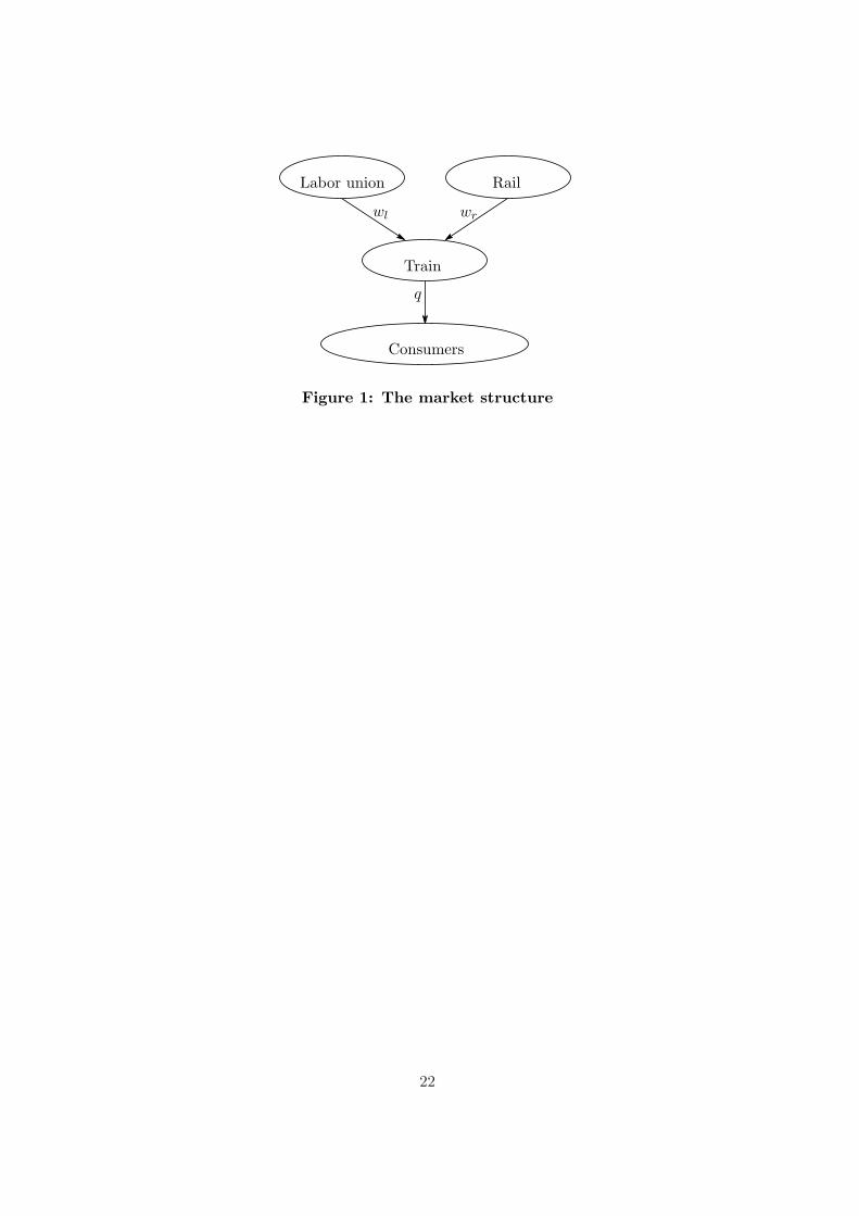
We explain the market structure in this paper.

There are three players related to train service provision to consumers. Firm T (Train

operating company) supplies some units of the train operation service to consumers. Firm R

(Rail infrastructure company) supplies an essential input (call it product r), in this case track

related to infrastructure, to firm T . Group L (Labor union) supplies labor (call it product l)

to firm T . Consumers enjoy the train travel service. Inverse demand for the service is given as

follows:

p = α − βq, (1)

where p is the price, q is the quantity supplied by firm T , and α and β are positive constants.3

Firm T needs one unit of product l and one unit of product r to produce one unit of train

travel service. Firm R and group L individually offer per unit wholesale price wr and per unit

wage of labor wl to firm T . The following figure depicts the market structure in this model.

[Figure 1 here]

Firm T generates a cost for firm R. The cost is positively correlated to the quantity supplied

by firm T , q. We assume that the cost is Cq where C is a positive constant.

structure affects the parties’ exposure to hold-ups. Che and Sakovics (2008) provided an excellent brief survey of

the hold-up problem. The topic of vertical foreclosure is also related to the problem of vertical integration. The

vertical foreclosure issue primarily concerns the relation between vertical integration and the competitiveness of

downstream firms (e.g., Ordover et al. (1990) and Hart and Tirole (1990)). See also O’Brien and Shaffer (1992),

McAfee and Schwartz (1994), Gaudet and Long (1996), Ma (1997), Riordan (1998), and Choi and Yi (2000).

Rey and Tirole (2007) provide an excellent survey of the literature.

3In Section 3.1, we use a more generalized demand function.

5

Let u briefly mention the cost structure in the railway industry. The role of a train operating

company (firm T ) is to provide service by running trains. Although the train operating company

holds rolling stock and employees such as engineers and conductors, this company borrows rail

tracks from a rail infrastructure company (firm R), to which it pays infrastructure charges.

The rail infrastructure company holds rail infrastructure, maintaining tracks and electrical

systems. Therefore, while the main costs of the train operating company are for labor, energy,

administration, rolling stock, and infrastructure rental, the main costs of the rail infrastructure

company are for track maintenance, electrical systems maintenance, and the depreciation of

infrastructure. We believe that this accurately summarizes the cost structure of this industry.

Firm R has an ability to reduce C through its effort. The constant C changes from c to c−e

if firm R pays its effort e and incurs the effort cost γe2 where c and γ are positive constants.

Assumption 1 To secure that the equilibrium price p is positive, we assume that βγ ≥ 1/3.

Given the quantity supplied by firm T is q, the consumer surplus is given as follows:

CS ≡∫ q

0(α − βm) dm − (α − βq)q =

βq2

2.

The social surplus is the sum of the consumer surplus and the total profits in this market.

We investigate the incentive of firms R and T to integrate vertically. To do so, we consider

two vertical structures: (1) Firms R and T are vertically separated; (2) Firms R and T are

vertically integrated.

Vertical separation When firms R and T are vertically separated, the objective functions

of the three players are given as follows:

πL = wlq, πT = (p − wl − wr)q, πR = wrq − (c − e)q − γe2.

In standard oligopoly models with labor unions, each downstream firm negotiates with its

labor union, which maximizes the product of its wage level and number of employees (for

examples, see Horn and Wolinsky (1988a,1988b), Davidson (1988), Dowrick (1989), Mumford

6

and Dowrick (1994), Naylor (2002), Lommerud et al. (2003), and Lommerud et al. (2009)).

The model used here is the standard one concerning the objective function of labor union.

In this case, the game runs as follows:

1. Group L and firm R offer per unit wage level (wl) and per unit wholesale price (i.e.,

infrastructure charge) (wr) to firm T .

2. Given the wage level and the wholesale price, firm R sets its effort level e and firm T sets

the amount of service q simultaneously.

Note that the timing of the game implies that firm R’s effort does not have a nature of

investment (credible commitment). If it has a nature of investment, the timing of the effort

choice should be earlier than that of wage setting. Firm R’s cost generated by firm T is related

to the operation of firm T . Firm R has to pay its daily effort to reduce this cost. To capture

the property of the cost-reducing efforts, we have assumed that the effort level e is determined

after the wage and the wholesale price are determined. We discuss how the timing structure

affects the decision of vertical integration/separation in Section 3.2.

Vertical integration When firms R and T are vertically integrated (call them firm I), the

objective functions of the two players are given as:

πL = wlq, πI = (p − wl)q − (c − e)q − γe2,

where I indicates the integrated firm. πI is the sum of πT and πR in the case of vertical

separation. The game runs as follows:

1. Group L offers per unit wage level (wl) to I.

2. Given the wage level, I sets its effort level e and the amount of service q simultaneously.

2.1 Vertical separation

We solve the game by backward induction.

7

In the second stage, the profits of firms T and R are given as:

πT = (α − βq − wl − wr)q,

πR = wrq − (c − e)q − γe2.

The first-order conditions of the firms lead to the quantity supplied by firm T and the effort

level of firm R given the wage level and the wholesale price:∂πT

∂q= α − 2βq − wl − wr = 0,

∂πR

∂e= q − 2γe = 0,

→

q(wl, wr) =

α − wl − wr

2β,

e(wl, wr) =α − wl − wr

4βγ.

In the first stage, anticipating the outcome in the second stage, group L and firm R maximize

their objectives:

πL = wlq(wl, wr) =wl(α − wl − wr)

2β,

πR = wrq(wl, wr) − (c − e(wl, wr))q(wl, wr) − γ(e(wl, wr))2

=(α − wl − wr)(α − wl + (8βγ − 1)wr − 8βγc)

16β2γ.

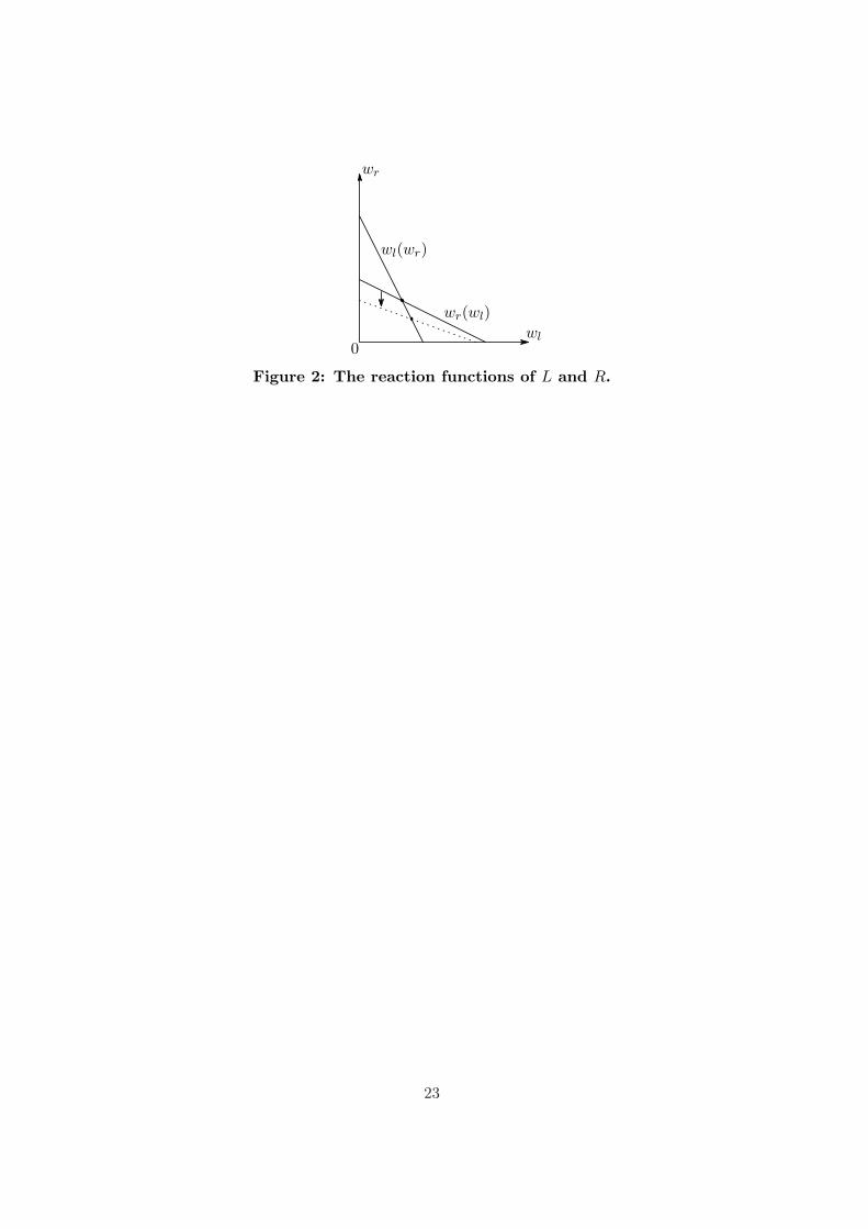
Their reaction functions are given by the following functions and summarized as Figure 2.

wl(wr) =α − wr

2, wr(wl) =

(4βγ − 1)α + 4βγc − (4βγ − 1)wl

8βγ − 1.

[Figure 2 here]

When the market size increases (i.e., a decrease in β), the reaction function of R moves down-

ward (see Figure 2). To understand the reason, we can rewrite the profit of firm R as follows:

πR = (wr − c)q(wl, wr) + {e(wl, wr)q(wl, wr) − γ(e(wl, wr))2}

=8β(wr − c)(α − wl − wr)

16β2γ+

(α − wl − wr)2

16β2γ.

The first term is the direct net profit through its input. The second term is the ‘gain’ from the

reduction of the negative externalities caused by firm T . This equation shows that an increase in

the market size (i.e., a decrease in β) enhances the relative importance of the gain from the cost

8

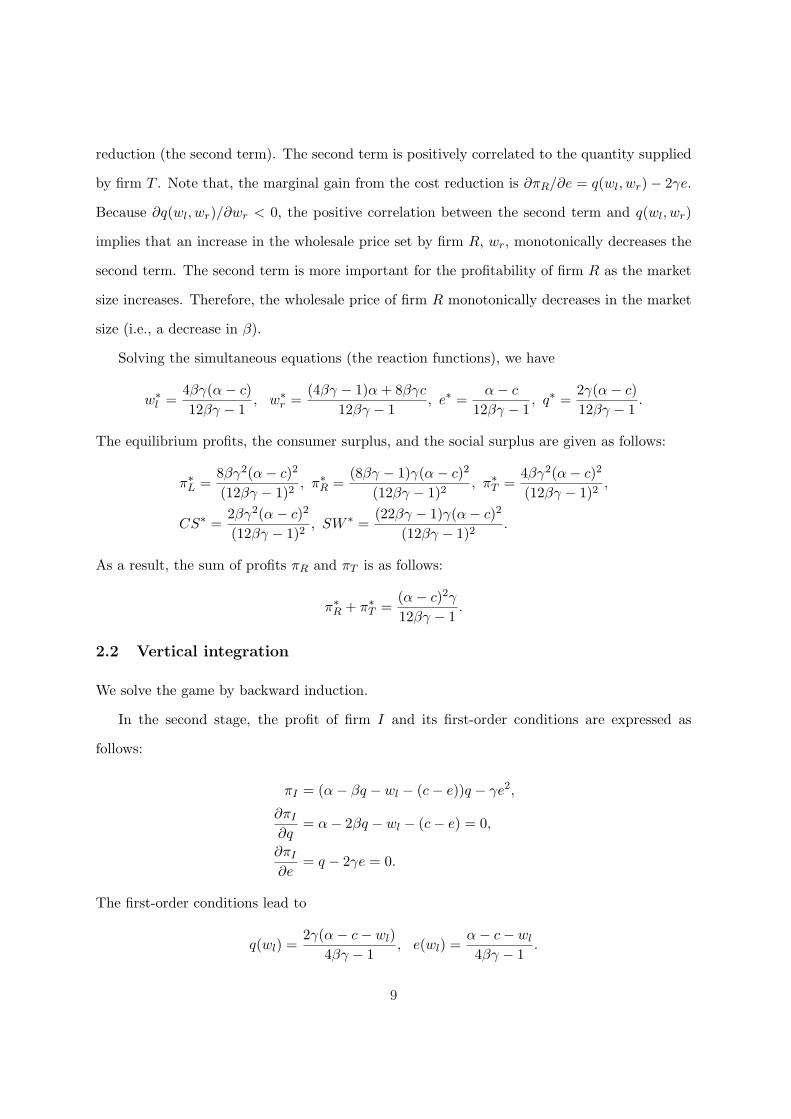
reduction (the second term). The second term is positively correlated to the quantity supplied

by firm T . Note that, the marginal gain from the cost reduction is ∂πR/∂e = q(wl, wr) − 2γe.

Because ∂q(wl, wr)/∂wr < 0, the positive correlation between the second term and q(wl, wr)

implies that an increase in the wholesale price set by firm R, wr, monotonically decreases the

second term. The second term is more important for the profitability of firm R as the market

size increases. Therefore, the wholesale price of firm R monotonically decreases in the market

size (i.e., a decrease in β).

Solving the simultaneous equations (the reaction functions), we have

w∗l =

4βγ(α − c)12βγ − 1

, w∗r =

(4βγ − 1)α + 8βγc

12βγ − 1, e∗ =

α − c

12βγ − 1, q∗ =

2γ(α − c)12βγ − 1

.

The equilibrium profits, the consumer surplus, and the social surplus are given as follows:

π∗L =

8βγ2(α − c)2

(12βγ − 1)2, π∗

R =(8βγ − 1)γ(α − c)2

(12βγ − 1)2, π∗

T =4βγ2(α − c)2

(12βγ − 1)2,

CS∗ =2βγ2(α − c)2

(12βγ − 1)2, SW ∗ =

(22βγ − 1)γ(α − c)2

(12βγ − 1)2.

As a result, the sum of profits πR and πT is as follows:

π∗R + π∗

T =(α − c)2γ12βγ − 1

.

2.2 Vertical integration

We solve the game by backward induction.

In the second stage, the profit of firm I and its first-order conditions are expressed as

follows:

πI = (α − βq − wl − (c − e))q − γe2,

∂πI

∂q= α − 2βq − wl − (c − e) = 0,

∂πI

∂e= q − 2γe = 0.

The first-order conditions lead to

q(wl) =2γ(α − c − wl)

4βγ − 1, e(wl) =

α − c − wl

4βγ − 1.

9

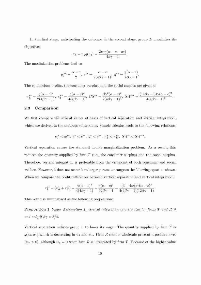
In the first stage, anticipating the outcome in the second stage, group L maximizes its

objective:

πL = wlq(wl) =2wlγ(α − c − wl)

4βγ − 1.

The maximization problems lead to

w∗∗l =

α − c

2, e∗∗ =

α − c

2(4βγ − 1), q∗∗ =

γ(α − c)4βγ − 1

.

The equilibrium profits, the consumer surplus, and the social surplus are given as

π∗∗L =

γ(α − c)2

2(4βγ − 1), π∗∗

I =γ(α − c)2

4(4βγ − 1), CS∗∗ =

βγ2(α − c)2

2(4βγ − 1)2, SW ∗∗ =

(14βγ − 3)γ(α − c)2

4(4βγ − 1)2.

2.3 Comparison

We first compare the several values of cases of vertical separation and vertical integration,

which are derived in the previous subsections. Simple calculus leads to the following relations:

w∗l < w∗∗

l , e∗ < e∗∗, q∗ < q∗∗, π∗L < π∗∗

L , SW ∗ < SW ∗∗.

Vertical separation causes the standard double marginalization problem. As a result, this

reduces the quantity supplied by firm T (i.e., the consumer surplus) and the social surplus.

Therefore, vertical integration is preferable from the viewpoint of both consumer and social

welfare. However, it does not occur for a larger parameter range as the following equation shows.

When we compare the profit differences between vertical separation and vertical integration:

π∗∗I − (π∗

R + π∗T ) =

γ(α − c)2

4(4βγ − 1)− γ(α − c)2

12βγ − 1=

(3 − 4βγ)γ(α − c)2

4(4βγ − 1)(12βγ − 1).

This result is summarized as the following proposition:

Proposition 1 Under Assumption 1, vertical integration is preferable for firms T and R if

and only if βγ < 3/4.

Vertical separation induces group L to lower its wage. The quantity supplied by firm T is

q(wl, wr) which is decreasing in wl and wr. Firm R sets its wholesale price at a positive level

(wr > 0), although wr = 0 when firm R is integrated by firm T . Because of the higher value

10

of wr in the case of vertical separation, the monopoly power of group L for firm T is weaker

than that in the case of vertical integration. This means that a portion of the monopoly profit

of group L is transferred to firm R through ‘competition’ between the complementary input

suppliers (Cournot (1838) and Sonnenschein (1968)). The rent-shifting from group L to firm R

is beneficial from the viewpoint of firms R and T . However, this effect depends on the market

size. As explained earlier, as the market size becomes larger (i.e., β becomes smaller), the

wholesale price of firm R, wR, becomes lower. This lower wholesale price allows group L to set

a higher wage, wL. This means that the rent-shifting effect is weak if the market size is large.

Therefore, the negative effect of coordination failure caused by vertical separation dominates

the positive effect of the rent-shifting if the market size is large (i.e., β is small).

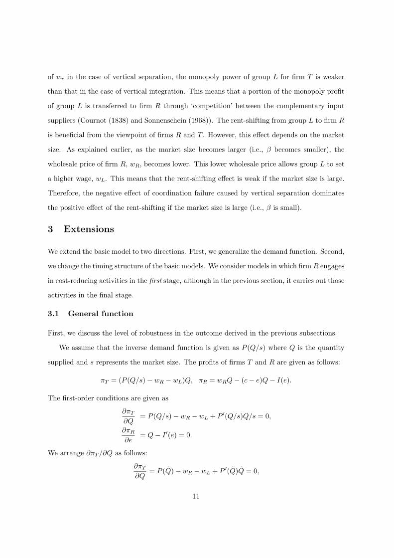
3 Extensions

We extend the basic model to two directions. First, we generalize the demand function. Second,

we change the timing structure of the basic models. We consider models in which firm R engages

in cost-reducing activities in the first stage, although in the previous section, it carries out those

activities in the final stage.

3.1 General function

First, we discuss the level of robustness in the outcome derived in the previous subsections.

We assume that the inverse demand function is given as P (Q/s) where Q is the quantity

supplied and s represents the market size. The profits of firms T and R are given as follows:

πT = (P (Q/s) − wR − wL)Q, πR = wRQ − (c − e)Q − I(e).

The first-order conditions are given as

∂πT

∂Q= P (Q/s) − wR − wL + P ′(Q/s)Q/s = 0,

∂πR

∂e= Q − I ′(e) = 0.

We arrange ∂πT /∂Q as follows:

∂πT

∂Q= P (Q) − wR − wL + P ′(Q)Q = 0,

11

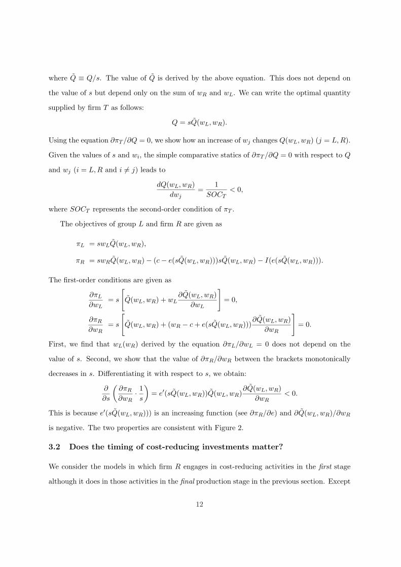
where Q ≡ Q/s. The value of Q is derived by the above equation. This does not depend on

the value of s but depend only on the sum of wR and wL. We can write the optimal quantity

supplied by firm T as follows:

Q = sQ(wL, wR).

Using the equation ∂πT /∂Q = 0, we show how an increase of wj changes Q(wL, wR) (j = L,R).

Given the values of s and wi, the simple comparative statics of ∂πT /∂Q = 0 with respect to Q

and wj (i = L,R and i = j) leads to

dQ(wL, wR)dwj

=1

SOCT< 0,

where SOCT represents the second-order condition of πT .

The objectives of group L and firm R are given as

πL = swLQ(wL, wR),

πR = swRQ(wL, wR) − (c − e(sQ(wL, wR)))sQ(wL, wR) − I(e(sQ(wL, wR))).

The first-order conditions are given as

∂πL

∂wL= s

[Q(wL, wR) + wL

∂Q(wL, wR)∂wL

]= 0,

∂πR

∂wR= s

[Q(wL, wR) + (wR − c + e(sQ(wL, wR)))

∂Q(wL, wR)∂wR

]= 0.

First, we find that wL(wR) derived by the equation ∂πL/∂wL = 0 does not depend on the

value of s. Second, we show that the value of ∂πR/∂wR between the brackets monotonically

decreases in s. Differentiating it with respect to s, we obtain:

∂

∂s

(∂πR

∂wR· 1s

)= e′(sQ(wL, wR))Q(wL, wR)

∂Q(wL, wR)∂wR

< 0.

This is because e′(sQ(wL, wR))) is an increasing function (see ∂πR/∂e) and ∂Q(wL, wR)/∂wR

is negative. The two properties are consistent with Figure 2.

3.2 Does the timing of cost-reducing investments matter?

We consider the models in which firm R engages in cost-reducing activities in the first stage

although it does in those activities in the final production stage in the previous section. Except

12

the timing structures, the structures of the games are the same with those in the previous

section. We explain the timing of the games.

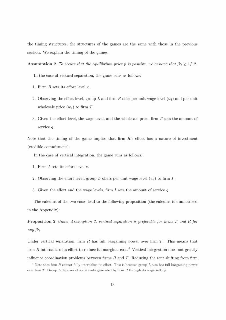
Assumption 2 To secure that the equilibrium price p is positive, we assume that βγ ≥ 1/12.

In the case of vertical separation, the game runs as follows:

1. Firm R sets its effort level e.

2. Observing the effort level, group L and firm R offer per unit wage level (wl) and per unit

wholesale price (wr) to firm T .

3. Given the effort level, the wage level, and the wholesale price, firm T sets the amount of

service q.

Note that the timing of the game implies that firm R’s effort has a nature of investment

(credible commitment).

In the case of vertical integration, the game runs as follows:

1. Firm I sets its effort level e.

2. Observing the effort level, group L offers per unit wage level (wl) to firm I.

3. Given the effort and the wage levels, firm I sets the amount of service q.

The calculus of the two cases lead to the following proposition (the calculus is summarized

in the Appendix):

Proposition 2 Under Assumption 2, vertical separation is preferable for firms T and R for

any βγ.

Under vertical separation, firm R has full bargaining power over firm T . This means that

firm R internalizes its effort to reduce its marginal cost.4 Vertical integration does not greatly

influence coordination problems between firms R and T . Reducing the rent shifting from firm4 Note that firm R cannot fully internalize its effort. This is because group L also has full bargaining power

over firm T . Group L deprives of some rents generated by firm R through its wage setting.

13

T to group L is more important from the viewpoint of the firms. Therefore, vertical separation

is always preferable.

This result is quite different from that in the previous section. In this section, the effort

cost of firm R is sunk before the wage and the wholesale price are determined. In the previous

section, however, cost is incurred when firm T sets its quantity supplied after the procurement

conditions are determined. This implies that a coordination problem exists between firms R

and T . The discussion in this section clarifies that, in the vertical structure discussed here, the

key factor of vertical integration is not the sunk-investment but the problem of coordination.

4 Concluding remarks

Vertically integrated and separated firms coexist in many industries, including railway. We have

provided an analytic framework to investigate this problem. We show that the downstream

firm which has the larger market size is more likely to integrate with the rail infrastructure firm.

This is consistent with the phenomenon in the Japanese railway industry. The result captures

the conjecture suggested by Williamson (1985, p. 94): A larger firm will also be more likely

to integrate if economies of scale in the “upstream” process result in lower costs for the large

firm’s own-production compared to a small firm. Because many empirical studies infer that

the hypothesis of transaction cost economics holds (Lafontaine and Slade (2007)), we believe

that our prediction can be applied to many economic environments.

As Proposition 1 states, if market size increases, vertical integration is preferable, as shown

in current empirical findings of Mizutani and Uranishi (2011) regarding the rail industry. By

applying the total cost function to 30 railway organizations from 23 OECD countries for the 14

years between 1994 and 2007, Mizutani and Uranishi (2011) evaluate whether or not vertical

separation caused a reduction in costs. The authors show that vertical separation effects with

lower train density tend to reduce the total cost of a railway organization but as train density

increases, vertical separation causes total costs to increase. This result means that vertical

integration is preferable in the case of high train density while vertical separation is preferable

in the opposite case. In their empirical analysis, train density is used but the measure (i.e.

14

train density) is highly related to market size. The definition of train density is measured by

how many trains run in a given railway network. If the market size is larger, then more train

services are required in the market. Therefore, if rail organizations have a large market, it

means that the rail organizations have larger train density. Thus, current empirical results

support our theoretical implication.

As mentioned above, while vertical separation is a common policy in the European Union,

vertical integration is still the structure of choice in the Japanese rail industry. Among vertical

separation options, there are many variations. Within the largely vertically separated Euro-

pean rail industry, opinions have been voiced against the separation policy. Keeping in mind

these various circumstances, we will provide theoretical background that may prove helpful in

evaluating vertical separation policy in the rail industry.

In conclusion, our theoretical results show that policy related to vertical separation depends

on market size, with vertical integration appropriate in rail organizations with a large market

and vertical separation preferable in organizations with a small market. Based on our theoret-

ical results, the European Commission’s policy, which is that vertical separation policy should

be applied everywhere, is not correct.

There are several ways to extend the monopoly model discussed here. Considering an

oligopoly model is a natural extension of the current model. For instance, we can consider

a situation in which two rail operation companies use the rails owned by two infrastructure

firms. In Japan, some vertically integrated railway companies use their own rails cooperatively

by operating their own trains from a terminal station owned by one of the companies to another

terminal station owned by the other company. We think that an extended model can capture

the essence of the Japanese and the EU railway industries and should be considered for future

research.

15

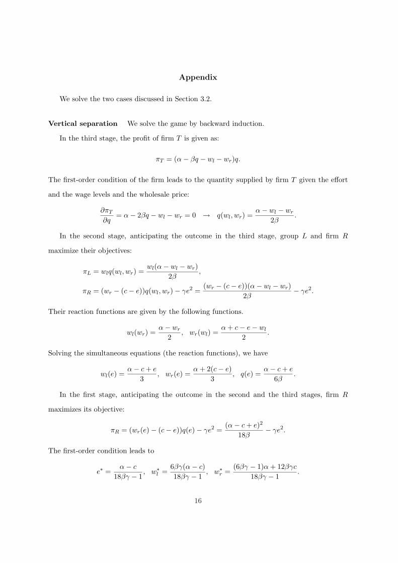
Appendix

We solve the two cases discussed in Section 3.2.

Vertical separation We solve the game by backward induction.

In the third stage, the profit of firm T is given as:

πT = (α − βq − wl − wr)q.

The first-order condition of the firm leads to the quantity supplied by firm T given the effort

and the wage levels and the wholesale price:

∂πT

∂q= α − 2βq − wl − wr = 0 → q(wl, wr) =

α − wl − wr

2β.

In the second stage, anticipating the outcome in the third stage, group L and firm R

maximize their objectives:

πL = wlq(wl, wr) =wl(α − wl − wr)

2β,

πR = (wr − (c − e))q(wl, wr) − γe2 =(wr − (c − e))(α − wl − wr)

2β− γe2.

Their reaction functions are given by the following functions.

wl(wr) =α − wr

2, wr(wl) =

α + c − e − wl

2.

Solving the simultaneous equations (the reaction functions), we have

wl(e) =α − c + e

3, wr(e) =

α + 2(c − e)3

, q(e) =α − c + e

6β.

In the first stage, anticipating the outcome in the second and the third stages, firm R

maximizes its objective:

πR = (wr(e) − (c − e))q(e) − γe2 =(α − c + e)2

18β− γe2.

The first-order condition leads to

e∗ =α − c

18βγ − 1, w∗

l =6βγ(α − c)18βγ − 1

, w∗r =

(6βγ − 1)α + 12βγc

18βγ − 1.

16

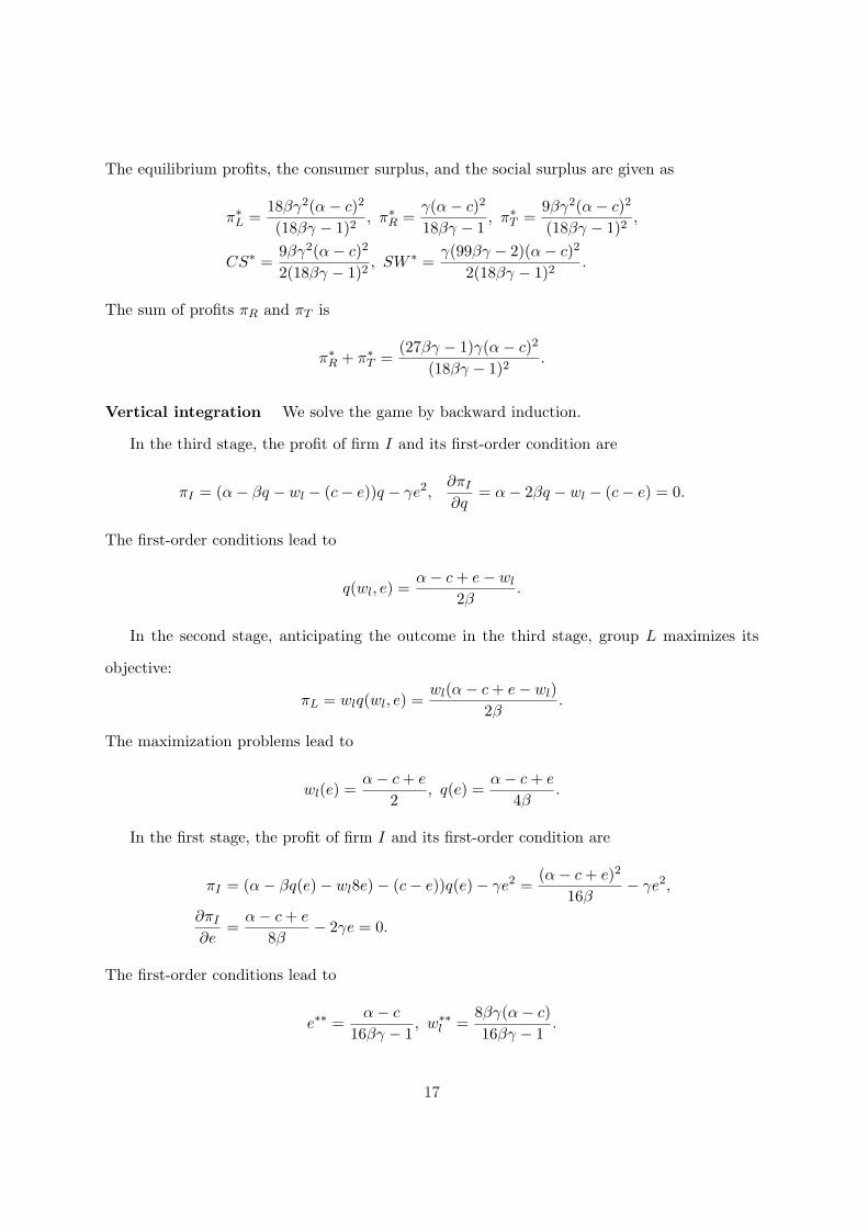
The equilibrium profits, the consumer surplus, and the social surplus are given as

π∗L =

18βγ2(α − c)2

(18βγ − 1)2, π∗

R =γ(α − c)2

18βγ − 1, π∗

T =9βγ2(α − c)2

(18βγ − 1)2,

CS∗ =9βγ2(α − c)2

2(18βγ − 1)2, SW ∗ =

γ(99βγ − 2)(α − c)2

2(18βγ − 1)2.

The sum of profits πR and πT is

π∗R + π∗

T =(27βγ − 1)γ(α − c)2

(18βγ − 1)2.

Vertical integration We solve the game by backward induction.

In the third stage, the profit of firm I and its first-order condition are

πI = (α − βq − wl − (c − e))q − γe2,∂πI

∂q= α − 2βq − wl − (c − e) = 0.

The first-order conditions lead to

q(wl, e) =α − c + e − wl

2β.

In the second stage, anticipating the outcome in the third stage, group L maximizes its

objective:

πL = wlq(wl, e) =wl(α − c + e − wl)

2β.

The maximization problems lead to

wl(e) =α − c + e

2, q(e) =

α − c + e

4β.

In the first stage, the profit of firm I and its first-order condition are

πI = (α − βq(e) − wl8e) − (c − e))q(e) − γe2 =(α − c + e)2

16β− γe2,

∂πI

∂e=

α − c + e

8β− 2γe = 0.

The first-order conditions lead to

e∗∗ =α − c

16βγ − 1, w∗∗

l =8βγ(α − c)16βγ − 1

.

17

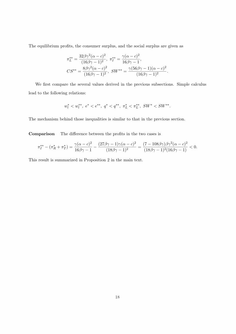
The equilibrium profits, the consumer surplus, and the social surplus are given as

π∗∗L =

32βγ2(α − c)2

(16βγ − 1)2, π∗∗

I =γ(α − c)2

16βγ − 1,

CS∗∗ =8βγ2(α − c)2

(16βγ − 1)2, SW ∗∗ =

γ(56βγ − 1)(α − c)2

(16βγ − 1)2.

We first compare the several values derived in the previous subsections. Simple calculus

lead to the following relations:

w∗l < w∗∗

l , e∗ < e∗∗, q∗ < q∗∗, π∗L < π∗∗

L , SW ∗ < SW ∗∗.

The mechanism behind those inequalities is similar to that in the previous section.

Comparison The difference between the profits in the two cases is

π∗∗I − (π∗

R + π∗T ) =

γ(α − c)2

16βγ − 1− (27βγ − 1)γ(α − c)2

(18βγ − 1)2=

(7 − 108βγ)βγ2(α − c)2

(18βγ − 1)2(16βγ − 1)< 0.

This result is summarized in Proposition 2 in the main text.

18

References

Arya, A., Mittendorf, B., and Sappington, D.E.M., 2008, ‘The Make-or-Buy Decision in thePresence of a Rival: Strategic Outsourcing to a Common Supplier’, Management Science54, pp. 1747–1758.

Baldwin, C.Y., and Woodard, C.J., 2007, ‘Competition in Modular Clusters’, Working Paper,Harvard Business School.

Beelaerts van Blokland, W.W.A., Verhagen, W.J.C., and Santema, S.C., 2008, ‘The Effects ofCo-Innovation on the Value-Time Curve: A Quantitative Study on Product Level’, Journalof Business Market Management 2, pp. 5–24.

Bonanno, G. and Vickers, J., 1988, ‘Vertical Separation’, Journal of Industrial Economics 36,pp. 257–265.

Casadesus-Masanell, R., Nalebuff, B., and Yoffie, D., 2007, ‘Competing Complements’, WorkingPaper, Harvard Business School.

Che, Y.-K. and Sakovics, J., 2008, ‘Hold-up Problem’, in Durlauf, S.N. and Blume, L.E. (eds.),The New Palgrave Dictionary of Economics, Second Edition, (Macmillan, London).

Chen, Y., 2001, ‘On Vertical Mergers and Their Competitive Effects’, RAND Journal of Eco-nomics 32, pp. 667–685.

Chen, Y., 2005, ‘Vertical Disintegration’, Journal of Economics and Management Strategy 14,pp. 209–229.

Choi, J. P. and Yi, S.-S., 2000, ‘Vertical Foreclosure with the Choice of Input Specifications’,RAND Journal of Economics, 31, pp. 717–743.

Coase, R. 1937, ‘The Nature of the Firm’, Economica 4, pp. 386–405.

Cournot, A. 1838, ‘Researches into the Mathematical Principles of the Theory of Wealth’,(Macmillan, New York); English translation, N. Bacon, 1897.

Davidson, C., 1988, ‘Multiunit Bargaining in Oligopolistic Industries’, Journal of Labor Eco-nomics 6, pp. 397–422.

Dowrick, S., 1989, ‘Union-Oligopoly Bargaining’, Economic Journal 99, pp. 1123–1142.

Economides, N. and Salop, S.C., 1992, ‘Competition and Integration Among Complements,and Network Market Structure’, Journal of Industrial Economics 40, pp. 105–123.

Gal-Or, E., 1999, ‘Vertical Integration or Separation of the Sales Function as Implied by Com-petitive Forces’, International Journal of Industrial Organization 17, pp. 641–662.

Gaudet, G. and Long, N.V., 1996, ‘Vertical Integration, Foreclosure, and Profits in the Presenceof Double Marginalization’, Journal of Economics and Management Strategy 5, pp. 409–432.

19

Grossman, S. and Hart, O., 1986, ‘The Costs and Benefits of Ownership: A Theory of Lateraland Vertical Integration’, Journal of Political Economy 94, pp. 691–719.

Grout, P. 1984, ‘Investment and Wages in the Absence of Binding Contracts: A Nash Bargain-ing Approach’, Econometrica 52, pp. 449–460.

Hart, O. and Moore, J., 1990, ‘Property Rights and the Nature of the Firm’, Journal of PoliticalEconomy 98, pp. 1119–1158.

Hart, O. and Tirole, J., 1990, ‘Vertical Integration and Market Foreclosure’, Brookings Paperson Economic Activity: Microeconomics, pp. 205–276.

Horn, H. and Wolinsky, A., 1988a, ‘Bilateral Monopolies and Incentives for Merger’, RANDJournal of Economics 19, pp. 408–419.

Horn, H. and Wolinsky, A., 1988b, ‘Worker Substitutability and Patterns of Unionization’,Economic Journal 98, pp. 484–497.

Klein, B., Crawford, R. and Alchian, A., 1978, ‘Vertical Integration, Appropriable Rents, andthe Competitive Contracting Process’, Journal of Law and Economics 21, pp. 297–326.

Lafontaine, F. and Slade, M., 2007, ‘Vertical Integration and Firm Boundaries: The Evidence’,Journal of Economic Literature 45, pp. 629–685.

Laussel, D., 2008, ‘Buying Back Subcontractors: The Strategic Limits of Backward Integration’,Journal of Economics and Management Strategy 17, pp. 895–911.

Lin, P., 2006, ‘Strategic Spin-Offs of Input Divisions’, European Economic Review 50, pp.977–993.

Lommerud, K.E., Meland, F., and Sørgard, L., 2003, ‘Unionised Oligopoly, Trade Liberalisationand Location Choice’, Economic Journal 113, 782–800.

Lommerud, K.E., Meland, F., and Straume, O.R., 2009, ‘Can Deunionization Lead to Interna-tional Outsourcing?’, Journal of International Economics 77, 109–119.

Ma, C.-T. A., 1997, ‘Option Contracts and Vertical Foreclosure’, Journal of Economics andManagement Strategy 6, pp. 725–753.

Maruyama, M. and Minamikawa, K., 2009, Vertical Integration, Bundled Discounts and Wel-fare, Information Economics and Policy 21, pp. 62–71.

Matsushima, N., 2009, ‘Vertical Merger and Product Differentiation’, Journal of IndustrialEconomics, 57, pp. 812–834.

Matsushima, N. and Mizuno, T., 2009, ‘Vertical Separation as a Defense Against Strong Sup-pliers’, ISER Discussion Paper 0755, Osaka University.

McAfee, R.P. and Schwartz, M., 1994, ‘Opportunism in Multilateral Vertical Contracting:Nondiscrimination, Exclusivity, and Uniformity’, American Economic Review 84, pp. 210–30.

20

Mizutani, F. and Uranishi, S., 2011, ‘Does Vertical Separation Reduce Cost? An EmpiricalAnalysis of the Rail Industry in OECD Countries,’ Discussion Paper Series No.2011-28,Graduate School of Business Administration, Kobe University.

Mumford, K. and Dowrick, S., 1994, ‘Wage Bargaining with Endogenous Profits, OvertimeWorking and Heterogeneous Labor’, Review of Economics and Statistics 76, pp. 329–336.

Nalebuff, B.J., 2000, ‘Competing Against Bundles’, in Peter J. Hammond and Gareth D.Myles, eds., Incentives, Organization, and Public Economics: Papers in Honour of SirJames Mirrlees pp. 323–336, (Oxford University Press, Oxford, UK).

Naylor, R.A., 2002, ‘Industry Profits and Competition under Bilateral Oligopoly’, EconomicsLetters 77, pp. 169–175.

O’Brien, D.P. and Shaffer, G., 1992, ‘Vertical Control with Bilateral Contracts’ RAND Journalof Economics 23, pp. 299–308.

Ordover, J., Saloner, G., and Salop, S., 1990, ‘Equilibrium Vertical Foreclosure’, AmericanEconomic Review, 80, pp. 127–142.

Rey, P. and Tirole, J., 2007, ‘A Primer on Foreclosure’, in Armstrong, M. and Porter, R.H.(eds.), Handbook of Industrial Organization, Vol. 3 (Elsevier, Amsterdam, The Nether-lands).

Riordan, M.H. 1998, ‘Anticompetitive Vertical Integration by a Dominant Firm’, AmericanEconomic Review 88, pp. 1232–1248.

Sonnenschein, H., 1968, ‘The Dual of Duopoly Is Complementary Monopoly: or, Two ofCournot’s Theories Are One’, Journal of Political Economy 76, pp. 316–318.

Tirole, J., 1986, ‘Procurement and Renegotiation’, Journal of Political Economy 94, pp. 235–259.

Williamson, O. 1979, ‘Transaction-Cost Economics: the Governance of Contractual Relations’,Journal of Law and Economics 22, pp. 233–262.

Williamson, O. 1985, The Economic Institutions of Capitalism: Firms, Markets, RelationalContracting, (The Free Press, New York, USA).

21

Labor union Rail

Train

Consumers

q

wl wr

Figure 1: The market structure

22

wl

wr

0

wl(wr)

wr(wl)

Figure 2: The reaction functions of L and R.

23