Market Segmentation and Software Security:

Pricing Patching Rights

Terrence August∗

Rady School of ManagementUniversity of California, San Diego

Korea University Business School

Duy Dao†

Rady School of ManagementUniversity of California, San Diego

Kihoon Kim‡

Korea University Business School

June 2018

Forthcoming in Management Science

Abstract

The patching approach to security in the software industry has been less effective than desired.One critical issue with the status quo is that the endowment of “patching rights” (the abilityfor a user to choose whether security updates are applied) lacks the incentive structure toinduce better security-related decisions. However, producers can differentiate their productsbased on the provision of patching rights. By characterizing the price for these rights, theoptimal discount provided to those who relinquish rights and have their systems automaticallyupdated in a timely manner, and the consumption and protection strategies taken by users inequilibrium as they strategically interact due to the security externality associated with productvulnerabilities, it is shown that the optimal pricing of these rights can segment the market in amanner that leads to both greater security and greater profitability. This policy greatly reducesunpatched populations and has a relative hike in profitability that is increasing in the extentto which patches are bundled together. Social welfare may decrease when automated patchingcosts are small because strategic pricing contracts usage in the market and also incentivizesloss-inefficient choices. However, welfare benefits when the policy either (i) greatly expandsautomatic updating in cases where it is minimally observed, or (ii) significantly reduces thepatching process burden of those who most value the software.

∗Rady School of Management, University of California, San Diego, La Jolla, CA 92093-0553. Visiting IlJinProfessor, Korea University Business School, Seoul, Korea, 136-701. e-mail: taugust@ucsd.edu

†Rady School of Management, University of California, San Diego, La Jolla, CA 92093-0553. e-mail:dddao@ucsd.edu@ucsd.edu

‡Korea University Business School, Seoul, Korea, 136-701. e-mail: kihoon@korea.ac.kr

1 Introduction

Patchable – but unpatched – vulnerabilities consistently allow attackers to compromise widely used

software such as systems provided by Microsoft, Adobe, and OpenSSL (US-CERT 2015). In fact,

64% of the top exploit samples in 2014 targeted patchable vulnerabilities from 2012 and prior

(HP Security Research 2015). As much as 85% of targeted security attacks could be prevented

by patching application and operating system vulnerabilities, in addition to employing whitelisting

and access control strategies, according to the Canadian Cyber Incident Response Centre (CCIRC

2014).

However, many users do not promptly install patches. Less than 29% of Windows operating

systems stay up to date according to OPSWAT, which collects data from software users through

its security platform (OPSWAT 2014). As a typical example, Microsoft released a patch on March

14, 2017, following revelation of a critical vulnerability’s existence (Microsoft 2017b). Two months

later, despite the patch having been made available, the WannaCry ransomware attack struck over

200,000 computers across over 150 countries that had not yet patched (Lohr and Alderman 2017,

Greenberg 2017). One month later and despite global media attention received by WannaCry,

many users and organizations had still not patched, and, as a result, the NotPetya ransomware was

able to spread by exploiting the same vulnerability (Microsoft 2017a).

In fact, many systems continue to remain unpatched long after patches are released. HP in-

dicates in its recent Cyber Risk Report 2015, that “... the majority of exploits discovered by our

teams attempt to exploit older vulnerabilities. By far the most common exploit is CVE-2010-2568,

which roughly accounts for a third of all discovered exploit samples” (HP Security Research 2015).

CVE-2010-2568, a Windows shell vulnerability that allows for remote code execution, was discov-

ered in June of 2010. The patch for this vulnerability was released weeks later in August of 2010.

Despite the patch being available for over six years, this vulnerability was still being exploited by

attackers at the time of the report.

Massive financial losses are being incurred directly by those whose unpatched systems get com-

promised. The WannaCry attack cost billions of dollars due to productivity losses, mitigation

efforts, paid ransom, and lost files (Berr 2017). In the case of NotPetya, a single organization,

Maersk, incurred direct losses in the range of $200-$300 million because the attack forced it to halt

shipping operations at 76 port terminals (Thomson 2017). Moreover, the presence of compromised

systems imposes indirect losses on all users. These systems can be leveraged in other criminal

1

activities such as spam (Levchenko et al. 2011), distributed denial-of-service attacks (Fitzgerald

2015), and even the conducting of click fraud campaigns (Ingram 2015).

Observing today’s cybersecurity attack landscape, the current patching process for security has

been less effective than desired (August et al. 2014). Why aren’t users patching? The growing

reality is that security is not a technical problem, it’s an economic one. Even though security

patches are available, many users are not deploying them because it is not in their economic best

interest to do so. For organizations, enterprise deployment of patches is a costly process. Extensive

testing of patches in development and staging environments, roll-out of updates onto production

servers, and final testing is both time consuming and resource intensive. Moreover, in aggregate

there is a deluge of patches that system administrators must continuously monitor and process. For

end users, the situation is regrettably similar because security patching is often not considered to be

a priority. The deployment of updates and system rebooting is instead viewed as an inconvenience,

particularly when users feel their own productivity is of greater concern.

Taking these costs into consideration, a software vendor can substantially increase security in an

incentive-compatible way by encouraging improved user behavior. In particular, it can differentiate

its software product by pricing patching rights.1 Specifically, the vendor should charge users for the

right to choose for themselves whether patches are installed or not installed on their systems. The

status quo is that all users are endowed with patching rights, and a substantial portion of them elect

not to patch as a result. By charging for patching rights, users who would otherwise have elected

not to patch under the status quo must now examine whether it is worth paying for this right

to remain unpatched. This decision is non-trivial as the expected security losses one would incur

when retaining rights and remaining unpatched depends on the security behaviors of all other

users in aggregate. On the flip side, by foregoing patching rights, users will have their systems

automatically (and immediately2) patched by the vendor, and pay a different price. However,

automatic deployment of patches also comes with risk because patches are not always stable. For

example, some users encounter the “Blue Screen of Death” when applying a patch from Microsoft

(Westervelt 2014, Sarkar and LeBlanc 2018). As another example of this risk, the cryptocurrency

1Our work is based on the original idea that patching rights should be managed. Having been first introducedqualitatively in a perspectives piece (August et al. 2014), our paper is the first to formally model and analyze thevalue of patching rights.

2In our study, automatic updates are assumed to be applied either immediately or within a reasonably shorttime frame so as to reduce security risk. This type of automatic update is consistent with those provided by manyleading software vendors (e.g., Microsoft, Oracle, Adobe, Google, etc.). There are some examples where firms manageautomatic updates but do so in an delayed manner, such as was the case with Apple taking three months to patchthe vulnerability exploited by the Flashback trojan (Hick 2012). This behavior is not in the spirit of the automatedpatching being modeled here.

2

exchange QuadrigaCX recently lost $14 million when inadequate patch testing failed to reveal that

their process of transferring ether (a cryptocurrency) was incompatible with an Ethereum client

software update (Higgins 2017). Considering these trade-offs, vendors have an incentive to target

certain users with lower prices in equilibrium in exchange for their patching rights, hence these

users will ultimately cause less of a security externality while benefitting from discounted software

prices.

Many researchers are working toward improving security and understanding why patch avail-

ability alone has not led to very secure outcomes; our work aims to contribute toward progress on

this front. In our model of security, users can choose whether to purchase a software product and

additionally whether to remain patched, unpatched, or have their systems automatically updated

in a timely manner by a software vendor. In this setting, examining the impact of optimally priced

patching rights (PPR) on security, profitability, and overall economic value gives rise to insights

that have promising practical implications to the software industry. Historically software compa-

nies have not differentiated on patching rights, but our insights may impel vendors to consider

how a more profitable, more secure ecosystem can be achieved as a result. A discussion of how

the essence of a PPR policy can be implemented as a component of a software vendor’s overall

versioning strategy follows our main results.

2 Literature Review

This work is related to three broad areas in the literature: (i) product differentiation and mar-

ket segmentation, (ii) economics of information security, and (iii) economics of product bundling.

With regard to the first stream, to the best of our knowledge, our paper is the first to examine

how beneficial segmentation in software markets can be constructed by differentiation on software

patching rights. More specifically, the focus is on a monopolist’s product mix/line decisions when

the quality-differentiated dimension concerns patching rights, as opposed to competition-driven

product differentiation. Within the second area, this work is most closely related to a strand that

studies the management of security patches. For the third area, our paper adds to a strand that

examines the impact of mixed bundling on a monopolist’s profit and social welfare.

Beginning with the first area, there is a well-developed literature in economics, marketing, op-

erations management and information systems that examines the monopolist’s problem of whether

to offer and how to price quality-differentiated goods. In this vein, classic papers focus on char-

3

acterizing the general optimal non-linear price schedule that incentivizes each consumer to select

the quality that is designed for her specific type (Mussa and Rosen 1978, Maskin and Riley 1984).

Subsequent literature explored how these schedules react to various changes in consumer charac-

teristics such as income dispersion and taste preferences (Moorthy 1984, Gabszewicz et al. 1986,

Desai 2001, Villas-Boas 2009), firm characteristics such as production technology and marketing

costs (Villas-Boas 2004, Debo et al. 2005, Netessine and Taylor 2007), and non-intrinsic charac-

teristics such as strategic delays (Moorthy and Png 1992, Chen 2001, August et al. 2015). Within

this body of work, our paper is most closely related to those that focus on consumer characteristics

in that an automated patching version essentially modifies the costs incurred by consumers.

There are two critical contributions that our model adds to this portion of literature. First,

the qualities that comprise product mix in our setting are endogenously determined in equilibrium

by consumption decisions; this is a significant context-specific trait where users who do not patch

their systems weakly reduce the quality of the software product for other users. Second, the

price schedule is not based on the product that gets consumed but rather the rights retained by the

consumer. Thus, our model admits interesting possibilities where consumers opt for the same rights

(giving access to the same quality level) but then separate based on their own subsequent patching

decisions (resulting in different effective qualities) – effective quality of the product is inclusive of

security attacks which are endogenously determined by the strategic protection behaviors employed

in equilibrium.

With regard to the second area of literature, our paper is close to work that studies the man-

agement of security patches. Researchers examine the timing of security patch release and its

application (Beattie et al. 2002, Cavusoglu et al. 2008, Dey et al. 2015), vulnerability disclosure

policy (Cavusoglu et al. 2007, Arora et al. 2008, Ransbotham et al. 2012), vendor patch policy

(Lahiri 2012 and Kannan et al. 2013), and users’ patching incentives (August and Tunca 2006,

Choi et al. 2010). Our work is closest to the latter group of papers which construct models that

endogenize users’ patching decisions. Consistent with this work and models of vaccination (see,

e.g., Brito et al. 1991), negative externalities stemming from unpatched behavior are modeled with

further generalization to include risk that is independent of patching populations. While interesting

in their own right, our model does not include other attack-related effects such as hiding effects

(Gupta and Zhdanov 2012), zero-day vulnerabilities (August and Tunca 2011), or strategic attack-

ers (Png and Wang 2009, Kannan et al. 2013). However, ours is the first to include both standard

and automated patching options for users while also modeling the security externality. Inclusion of

4

automated patching permits a characterization of the natural consumer market segmentation that

arises in equilibrium as users strategically respond to security risk and expanded patching options.

An understanding of equilibrium consumption and security behavior serves to inform how security

enhancements should be marketed. Also, an automated patching option is the logical choice for the

baseline product in a policy where patching rights are contracted, which is the focus of our work.

Toward addressing users’ incentives, August and Tunca (2006) examine the efficacy of patching

rebates. Patching rebates work by having the vendor subsidize patching costs in order to get more

users to patch rather than remaining unpatched and contributing to security risk. August and

Tunca (2006) show that these rebates can be very effective at improving behavior and security.

They also show that if standard patching costs are large, it is not efficient to incentivize lower

valuation users to incur these costs. One nice feature of the PPR policy is it does not require

lower valuation users to incur these patching costs. Rather, it incentivizes them to have patches

automatically deployed and instead incur potential system instability losses due to automated

deployment. Since these losses tend to be lower, PPR works by incentivizing these users to engage

in more appropriate and economical patching behaviors.

Finally, our work is related to a third body of literature examining a monopolist’s decision

regarding pure and mixed bundling. Under a PPR policy, software is unbundled from the right to

decide whether or not to apply security patches.3 There exists a well-developed literature on the

bundling of physical products and information goods spanning the fields of economics, marketing,

and information systems. Under moderate costs associated with automated patching, our proposed

partial mixed bundling scheme (PPR) can simultaneously improve the software vendor’s profit

as well as security relative to the pure bundling alternative status quo. Several related works

share the similar qualitative conclusion in which mixed bundling is favored over pure bundling

and unbundled sales (see, e.g., Adams and Yellen 1976, Schmalensee 1984, McAfee et al. 1989,

Venkatesh and Kamakura 2003). These works show that bundling effectively extracts consumer

surplus under various distributions of reservation values. In our work, partial mixed bundling when

involving patching rights can possibly result in a slight decrease in social welfare, but it can also

drive increases in social welfare depending on the quality of automated patching solutions and the

extent to which security risk is reduced.

3The status quo of providing software bundled with patching rights is in a sense pure bundling. PPR is partialmixed bundling: a bundle of software with patching rights and software alone without patching rights (Stremerschand Tellis 2002). Because patching rights have no standalone value, mixed bundling does not include the sale ofpatching rights.

5

In comparison to physical goods, information goods are typically assumed to have zero marginal

costs, which enable the monopolist to bundle many information goods economically; this makes

sense particularly when their valuations are correlated (Bakos and Brynjolfsson 1999). If two infor-

mation goods provide highly asymmetric values to consumers, partial mixed bundling is optimal;

the higher valuation good should not be sold separately not to cannibalize the sale of the bundle

(Eckalbar 2010, Bhargava 2013). Idiosyncratic to our context, patching rights cannot be sold sepa-

rately because they only have value to those who buy software. Unlike prior work on bundling, our

model involves a security externality from unpatched software usage. Partial mixed bundling of

two information goods has been shown to be optimal when only one good has a direct externality

on consumer utility (Prasad et al. 2010). However, in our model, as more consumers purchase the

automated patching version, other consumers become more willing to pay for the bundled version

with patching rights due to the increased level of security.

3 Model Description and Consumer Market Equilibrium

3.1 Model

There is a continuum of consumers whose valuations of a software product lie uniformly on V =

[0, 1]. Consumers are exposed to security risks associated with the software’s use. In particular, a

vulnerability can arise in the software, in which case the vendor makes a security patch available

to all users of the software. Because the security vulnerability can be used by malicious hackers to

exploit systems, users who do not apply the security patch are at risk.

The vendor offers two options for users to protect their respective systems. In doing so, the ven-

dor prices the software based on whether patching rights are granted to the consumer. Specifically,

if a consumer elects to purchase the software and retain full patching rights, she pays the price

p≥ 0. Having this right means that she can choose whether to patch the software or not patch the

product and do so according to her own preferences. If she decides to patch the software, she will

incur an expected cost of patching denoted cp> 0. This standard patching cost accounts for the

money and effort that a consumer must exert in order to verify, test, and roll-out patched versions

of existing systems.4

4Standard patching processes require considerable care, essentially coming down to labor costs associated withsystem administrators and developers spending time to complete all of the tasks in the patching process (Beres andGriffin 2009). Studies find that standard patching costs tend to be on the order of one thousand dollars per server(Bloor 2003, Forbath et al. 2005, Beres and Griffin 2009). Modeling the cost of standard patching as a constantis common in the literature that examines topics related to patching costs as can be seen in Beattie et al. (2002),

6

If she decides not to patch the software, then she faces the risk of an attack. Two classes of

security losses are incurred: (i) those that are dependent on the size of the unpatched population

of users, and (ii) those that are independent of the unpatched population size. For the dependent

case, if she decides not to patch the software, the probability she is hit by a security attack is given

by πsu, where πs ∈ (0, 1] is the probability an attack appears and u is the size of the unpatched

population of users.5 This reflects the negative security externality imposed by unpatched users of

the software. If she is successfully attacked, then she will incur expected security losses that are

positively correlated with her valuation. For simplicity, the correlation is assumed to be of first

order, i.e., the loss that a consumer with valuation v suffers if she is hit by an attack is αsv where

αs > 0 is a constant. The quantity πsαs is referred to as dependent risk throughout the paper.

The dependent case directly captures any attack that spreads through vulnerable populations and

is agnostic to the specific attack vector or mechanism by which spreading occurs.

The dependent case also indirectly captures any type of security attack where the incentives of

the malicious individual for constructing the attack is positively related to the unpatched population

size. For example, if large vulnerable populations are more attractive to hackers because it becomes

easier to penetrate hosts or the return on their efforts becomes higher when infecting more hosts,

then the dependent case applies. On the other hand, unpatched users can also face risk from attacks

that are independent of the size of the unpatched population. This class can include targeted attacks

and other forms of background risk. Using analogous notation, the likelihood of an independent

attack is denoted by πi ∈ (0, 1], and similarly πiαi is referred to as independent risk, where αi > 0

is a constant.

If the consumer instead elects to purchase the software and relinquish patching rights, she pays

the price δp, where δ≥ 0. In this case, the vendor retains full control over patching the software

and will automatically and immediately do so to better protect the user population.6 From an

implementation point of view, this software version would not give users much or any control over

patch deployment (e.g., the typical options can be grayed out in this version). The user incurs a

cost of automated patching, ca> 0, which is associated with both inconvenience and configuration

August and Tunca (2006), Choi et al. (2010) and Cavusoglu et al. (2008).5The size of the unpatched population u is determined by the consumer strategies in equilibrium. Therefore, by

the definition of V, u∈ [0, 1].6This is fairly easy to enforce in interconnected networks. For example, vendors such as Adobe and Matlab enforce

real-time license checks for their subscription-based offerings. While it is always possible to circumvent protections,most paying customers are unlikely to break the license agreement. Our model assumes immediate patch deploymentfor simplicity. The essence of our results only require that patchers, whether automated or standard, complete tasksin a relatively timely manner that distinguishes them from those who do not patch.

7

of the system to handle automatic deployment of security patches.7 There is always some risk

associated with an automatically deployed patch causing a user’s system to become unstable or

even crash because a vendor cannot test for compatibility of the patch with every possible user

system configuration. This probability that the automated patch is problematic is denoted by

πa ∈ (0, 1]. The loss associated with an automated patch deployment failure is again positively

correlated with her valuation. Assuming first-order correlation, denoted αa> 0, her expected loss

associated with automated patching is given by πaαav.8

Each consumer decides whether to buy, B, or not buy, NB. Similarly, for her patching de-

cision, she chooses one of patch, P , not patch, NP , and automatically patch, AP . In order to

choose P or NP , she must pay the price p to retain patching rights. By choosing AP , she delegates

patching rights to the vendor and pays the price δp. The consumer action space is then given by

S=({B}× {P,NP,AP}) ∪ (NB,NP ). In a consumer market equilibrium, each consumer maxi-

mizes her expected utility given the equilibrium strategies for all consumers. For a given strategy

profile σ : V → S, the expected utility for consumer v is given by:

U(v, σ)�

⎧⎪⎪⎪⎪⎪⎪⎨⎪⎪⎪⎪⎪⎪⎩

v − p− cp if σ(v)= (B,P ) ;

v − p− πsαsu(σ)v − πiαiv if σ(v)= (B,NP ) ;

v − δp− ca − πaαav if σ(v)= (B,AP ) ;

0 if σ(v)= (NB,NP ) ,

(1)

where

u(σ)�∫V11{σ(v) = (B,NP )} dv . (2)

To avoid trivialities and without loss of generality, the parameter space is reduced to cp, ca ∈ (0, 1)

and πaαa ∈ (0, 1 − ca), which ensures automated patching is economical.

7Our model can examine any relationship between cp and ca. For example, it can capture the commonly observedsituation in which users are choosing between: (i) completing all tasks associated with the rigorous, standard patchingapproach and incurring cp, or (ii) doing the bare minimum to deploy patches automatically without verification andincurring a lower cost, ca <cp, related to deployment. The model can also handle situations where ca ≥ cp, to studyscenarios in which users aim to achieve all tasks associated with standard patching but in an automated manner.

8The loss factor πaαa captures in expectation major patch failures that would lead to severe backlash against thevendor. An increased likelihood of such events is represented by a higher πaαa, which will affect the value of a PPRpolicy.

8

3.2 Consumer Market Equilibrium

Before examining how patching rights should be priced, it is necessary to characterize how con-

sumers segment across strategies for an arbitrary set of prices in equilibrium. Endogenous deter-

mination of the security externality that results from usage and patching decisions complicates the

situation. The consumer with valuation v selects an action that solves the following maximization

problem:

maxs∈S

U(v, σ) , (3)

where the strategy profile σ is composed of σ−v (which is taken as fixed) and the choice being

made, i.e., σ(v) = s. Her optimal action that solves (3) is denoted s∗(v). The equilibrium strategy

profile is denoted σ∗, and it satisfies the requirement that σ∗(v) = s∗(v) for all v ∈V.

Lemma 1 There exists a unique equilibrium consumer strategy profile σ∗ that is characterized by

thresholds vb, va, vp ∈ [0, 1]. For each v ∈V, it satisfies either

σ∗(v) =

⎧⎪⎪⎪⎪⎪⎪⎨⎪⎪⎪⎪⎪⎪⎩

(B,P ) if vp<v≤ 1 ;

(B,NP ) if vb<v≤ vp ;

(B,AP ) if va<v≤ vb ;

(NB,NP ) if 0≤ v≤ va ,

(4)

or

σ∗(v) =

⎧⎪⎪⎪⎪⎪⎪⎨⎪⎪⎪⎪⎪⎪⎩

(B,P ) if vp<v≤ 1 ;

(B,AP ) if va<v≤ vp ;

(B,NP ) if vb <v≤ va ;

(NB,NP ) if 0≤ v≤ vb .

(5)

Lemma 1 establishes that if a population of patched consumers arises in equilibrium, it will

consist of a segment of consumers with the highest valuations. These consumers prefer to shield

themselves from any valuation-dependent losses born when either remaining unpatched (security

losses) or using automated patching (instability losses). Importantly, this segment need not arise

(e.g., the upper threshold satisfies vp=1 in cases where valuation-dependent losses are smaller than

patching costs). The middle segments, composed of consumers who elect for automated patching

or to remain unpatched, can be ordered either way depending on the relative strength of the losses

under each strategy.

9

4 Pricing Patching Rights

Since the value of patching is most applicable under higher security risk, our study centers on regions

such that patching is worthwhile (i.e., either independent risk or dependent risk is reasonably

high). There are several merits to begin analysis with high independent risk. First, based on

user incentives, this case is inherently simpler and ultimately admits closed-form solutions of the

consumer market thresholds and prices that arise in equilibrium. This helps build intuition into

how a PPR policy tends to affect equilibrium behaviors. Second, the impact of high independent

risk is similar in nature to that of high dependent risk in that both tend to reduce unpatched

populations as users become unwilling to bear higher risk. In this light, certain limit effects on

thresholds and profitability will be the same and can be characterized more easily in a simplified

setting. Third, examination of this case underscores why capturing dependent risk is essential to a

comprehensive understanding of interdependent security settings, which propels the remainder of

the paper.

4.1 High Independent Risk

For convenience, parameter sets satisfying πiαi > 1 are examined as a proxy for the case of high

independent risk. Section A of the Appendix provides a complete characterization of the parameter

conditions and thresholds for each possible consumer market structure that can arise in equilibrium.

There are three possible structures, with the two most relevant to the current discussion having

threshold orderings given by 0<va<vp< 1 and 0<vp< 1. These two structures obtain under

broad conditions which, in turn, can be satisfied under equilibrium pricing decisions. Under high

independent risk, no user will elect to be unpatched, which is to say there is no security externality

in equilibrium.

Turning toward equilibrium pricing, the vendor’s profit function is given by

Π(p, δ) = p

∫V1{σ∗(v|p,δ)∈{(B,NP ),(B,P )}}dv + δp

∫V1{σ∗(v|p,δ)=(B,AP )}dv , (6)

noting that marginal costs are assumed to be negligible for information goods. Given an interest

in determining the benefit of optimally pricing the right for a user to determine whether or not

to install patches on her system, it is useful to first present a characterization of the equilibrium

when this right is not priced. In this reference case, referred to throughout the paper as the status

quo, standard practice for the industry is that δ=1 such that the price is the same regardless

10

of patching behavior. In this case, the vendor chooses a price p for the software by solving the

following problem:

maxp∈[0,∞)

Π(p, δ)

s.t. (vb, va, vp) are given by σ∗(· | p, δ),δ=1.

(7)

Given a price p∗ that solves (7), the profit associated with this optimal price are denoted by

ΠSQ � Π(p∗, 1).

Lemma 2 (Status Quo) Suppose that πiαi> 1 and δ=1 (i.e., when patching rights are not

priced).

(i) If cp − πaαa < ca < 1− πaαa − (1− cp)√1− πaαa, then

p∗ =1− πaαa − ca

2, (8)

and σ∗ is characterized by 0<va<vp< 1 such that the lower tier of users prefers automated

patching.

(ii) On the other hand, if ca ≥ 1− πaαa − (1− cp)√1− πaαa, then

p∗=1− cp

2, (9)

and σ∗ is characterized by 0<vp< 1 such that there is no user of automated patching in

equilibrium.

Lemma 2 presents the equilibrium behavior under the status quo reference case. Part (i)

establishes that as long as the cost of standard patching (cp) and automated patching (ca) satisfy

conditions where ca is moderate, both standard patching and automated patching are observed

strategies in equilibrium. On the other hand, as ca increases to a higher level, only standard

patching is observed. Lemma 2 highlights that high independent risk essentially squeezes out

unpatched behaviors, leading to the absence of a security externality in equilibrium. It is useful

to understand the role of PPR in this context as it will serve as a contrastable reference point for

when externalities become a driving force.

When patching rights are priced, the vendor jointly selects a price and multiplier (p, δ) to

11

maximize his profits. His pricing problem is formulated as follows:

max(p,δ)∈[0,∞)2

Π(p, δ)

s.t. (vb, va, vp) are given by σ∗(·|p, δ).(10)

Under the optimal choices (p∗, δ∗) which solve (10), the optimal profit under priced patching rights

is denoted by ΠP �Π(p∗, δ∗).9

Lemma 3 (PPR) Suppose that πiαi> 1 and patching rights are priced by the vendor.

(i) If cp − πaαa < ca < cp(1− πaαa), then

p∗ =1− cp

2, (11)

δ∗ =1− ca − πaαa

1− cp, (12)

and σ∗ is characterized by 0<va<vp< 1 such that the lower tier of users prefers automated

patching.

(ii) On the other hand, if ca ≥ cp(1− πaαa), then

p∗=1− cp

2, (13)

δ∗ = 1, (14)

and σ∗ is characterized by 0<vp< 1 such that there is no user of automated patching in

equilibrium.

Lemma 3 formally establishes that PPR can greatly expand the region of the parameter space

on which automated patching is observed, relative to the status quo. Specifically, when the condi-

tion 1− πaαa − (1− cp)√1− πaαa≤ ca<cp(1− πaαa) is satisfied, then automated patching arises

(0<va<vp< 1) when patching rights are priced whereas it does not arise (0<vp< 1) in the status

quo. When part (i) of Lemma 3 is satisfied, then patching rights are priced in a way that consumers

who select automated patching in equilibrium form the lower tier of the consumer market. In equi-

librium, the vendor charges the “premium” p∗(1− δ∗) for patching rights; alternatively, p∗(1− δ∗)9Going forward, subscripts “SQ” and “P” indicate a particular measure refers to the outcome under the status

quo and under a PPR policy, respectively, for consistency.

12

can be considered the “discount” given to users who agree to have their systems automatically

updated to reduce security risk.

By (11) and (12), it is easy to see that the premium charged for patching rights is only greater

than the cost of automated patching (ca) when standard patching costs (cp) are small enough. To

understand why, the software vendor has an incentive to charge a high price for his software when

standard patching costs are small. One can think of his product as being better software that is

easily maintained via a cost-effective, rigorous patching process. Therefore, the vendor can achieve

a sizable user population, most of which elects for standard patching, even when charging a high

price. Because of the attractiveness of standard patching, it is necessary to provide a significant

discount to incentivize users to prefer the automated patching option. This is reflected in (12);

the optimal price multiplier (δ∗) decreases as standard patching costs (cp) decrease. From the

other perspective, the patching rights premium p∗(1 − δ∗) is substantial and can be an incentive-

compatible option only for high-valuation users. Low-valuation users necessarily find the patching

rights premium too high to bear and instead opt for automated patching in equilibrium.

Proposition 1 When πiαi > 1, if cp − πaαa<ca< 1 − πaαa − (1 − cp)√1− πaαa, the relative

increase in profitability of pricing patching rights is given by

ΠP −ΠSQ

ΠSQ=

(1− πaαa)(ca − cp + πaαa)2

πaαa(1− ca − πaαa)2, (15)

where

ΠSQ =(1− ca − πaαa)

2

4(1− πaαa). (16)

Proposition 1 formally establishes the extent to which a PPR policy can increase profitability for

the vendor. In the context of our overall study, what is important to emphasize here is that the

vendor can have strong incentives to leverage an automated patching version toward discriminatory

purposes. In particular, under high independent risk, Lemmas 2 and 3 establish that no unpatched

usage arises in equilibrium and so it is not the case that the PPR policy being employed aims to

reduce the security externality. The segmentation behavior seen here solely targets extraction of

surplus from high-valuation users by inducing them to pay the patching rights premium. These

users have much to lose in the event of any system failure occurring due to patch instability, and thus

are willing to pay to retain control and continue to exercise diligence in their patching processes.

Users whose valuations are not high will find it incentive-compatible to relinquish patching

rights. In fact, a sizable segment of consumers switch from standard patching towards automated

13

patching when patching rights are priced. As the proofs of part (i) of Lemmas 2 and 3 establish,

the user type indifferent between using automated patching and not even buying the software (va)

is identical both in the status quo and under PPR. Viewed in that light, the pricing of patching

rights does not expand usage in the market, instead only serving to encourage some users to make

less loss-efficient security choices yet benefitting vendor profitability.

This proposition also shows that a PPR policy always outperforms a mandated automated

patching policy. The reason is because mandating automated patching is a special case of a priced

patching rights policy. Specifically, the decision problem when mandating automatic patching can

be formulated in the same manner as the PPR problem, subject to an additional constraint that

the price of patching rights is prohibitively high (i.e., p = 1). As seen in the utility function given

by (1), setting such a price makes the strategies of being unpatched (B, NP ) and using standard

patching processes (B, P ) infeasible to consumers, and the vendor chooses a price multiplier (δ) to

maximize profits with all consumers now only considering automated patching (B, AP ). Because

the price p = 1 is feasible but never chosen in the original problem, mandating automatic patching

leads to strictly lower profits.

A vendor’s patch release frequency impacts PPR’s relative profitability. A frequent patch release

policy imposes additional burden on those who follow a standard patching policy. In our model

abstraction, higher frequency corresponds to higher standard patching costs (i.e., higher cp). By

equation (15), the relative profitability of PPR is decreasing in standard patching costs. Because

higher standard patching costs naturally incentivize users to shift toward automated patching usage

rather than unpatched usage (due to high independent risk πiαi), the upside of PPR becomes

limited. More frequently released patches can also reduce costs associated with patch instability

because problems are much easier to diagnose when scope is narrower. In (15), relative profitability

is similarly decreasing as instability risk (πaαa) decreases. Overall, the relative value of PPR is

generally higher when patches tend to be bundled together.

Proposition 1 highlights the discriminatory forces at work when the vendor can separately price

an automated patching version of his product without being concerned about security externalities.

On the other hand, equilibrium consumer market outcomes marked by no user being unpatched

call attention to the source of the risk. In particular, one might ponder why independent risk (πiαi)

is high if nobody is unpatched. Even if only a few users out of a large population were unpatched,

should we expect them to face high risk? This line of thought suggests that security risk and the

size of the unpatched population may naturally have some dependence which is the focus of the

14

next section.

4.2 Low Independent Risk

When independent risk is more moderate in nature (i.e., explicitly bounded above), equilibrium

outcomes now differ under high dependent risk. In contrast to the prior section, in equilibrium there

exists a segment of unpatched users regardless of dependent risk being high. The characterization of

the thresholds that emerge in the equilibrium consumer market structure become significantly more

complex, satisfying a nonlinear system of equations. Therefore, asymptotic analysis is employed,

which is commonly found in microeconomic studies.10

As before, it is helpful to first characterize the consumer market equilibrium when patching

rights are freely included.

Lemma 4 (Status Quo) There exists αs such that when αs> αs, if πiαi < min[

cpπaαa

1+cp−ca,

cp1+cp

],

δ=1 (i.e., when patching rights are not priced),

(i) if cp − πaαa < ca < 1− πaαa − (1− cp)√1− πaαa, then

p∗ =1

2(1−πaαa−ca)+

2c2a(πaαa − 1)((πaαa − 1)(2πaαa − πiαi − 1) + ca(2πaαa + πiαi − 3))

(−πaαa + ca + 1)3πsαs+Ka ,

(17)

and σ∗ is characterized by 0<vb <va<vp< 1 such that the lower tier of users remain un-

patched and the middle tier prefers automated patching.

(ii) On the other hand, if ca > 1− πaαa − (1− cp)√1− πaαa, then

p∗=1− cp

2− 2c2p(1− 3cp + πiαi(1 + cp))

(1 + cp)3πsαs+Kb , (18)

and σ∗ is characterized by 0<vb <vp< 1 such that there is no user of automated patching in

equilibrium.11

10Its use can be expected here due to the complexity of the game and corresponding equilibrium characterization(some examples of studies using asymptotic analysis include Li et al. 1987, Laffont and Tirole 1988, MacLeod andMalcomson 1993, Pesendorfer and Swinkels 2000, Muller 2000, Tunca and Zenios 2006, August and Tunca 2006, Peiet al. 2011 among many others). Miller (2006) and Cormen et al. (2009) provide comprehensive treatments of themathematical foundation underlying asymptotic analysis. Due to model complexity in this region, some boundaries donot have explicit functional forms. However, the objective of the analysis is the identification of regions of applicabilityin terms of parameter characteristics, which is the focus of our formalized results.

11The existence of αs is proven in the Appendix. The characterization of constants denoted by K and enumeratedby a subscript are similarly provided.

15

Part (i) of Lemma 4 provides the reference case when the cost of automated patching is relatively

moderate. An immediate observation is that when patching rights are free as in the status quo, the

consumer segment whose equilibrium strategy is to use automated patching is always the middle

tier. This occurs because when a user compares an automated patching strategy to an unpatched

strategy, the price is the same for both options. Therefore, the former strategy is preferred to the

latter as long as the condition v[πsαsu(σ∗)+πiαi−πaαa]>ca is satisfied. Notably, this condition is

monotone in v which is to say that if it is satisfied for any user with valuation v, it is also satisfied

for any user with a valuation higher than v. As a result, the automated patching segment of users

always form the middle tier. Contrasting this to the previous section, under high independent

security risk the automated patching segment formed the lowest tier. This cannot happen in the

current region when patching rights are endowed.12

These observations highlight an important potential impact of a PPR policy; if the premium

charged for patching rights, p(1 − δ), is greater than the cost of automated patching (ca) and the

unpatched population, u(σ∗), decreases enough in equilibrium, then the lower tier can instead be

composed of users who strategically choose automated patching. In this sense, a PPR policy can

fundamentally change segmentation behavior in the consumer market, which in turn can have a

significant impact on security and profitability. The following lemma formalizes the equilibrium

strategies under PPR.

Lemma 5 (PPR) Suppose that αs> αs, πiαi < min[

cpπaαa

1+cp−ca,

cp1+cp

], and that patching rights are

priced by the vendor.

(i) If ca < min [πaαa − cp, cp(1− πaαa)], then

p∗ = p+

(2πaαacp

(πiαic

2a + ca(−πaαaπiαi + 3πaαacp − 2cpπiαi) + cp(πaαa(πaαa + πiαi)+

cp(πiαi − 3πaαa))))(

πsαs(−πaαa + ca − cp)3

)−1

+Kc, (19)

12Under low independent risk whenever a standard patching population arises in equilibrium, there must also be apopulation of unpatched users. Otherwise, a standard patching user would deviate to being unpatched and bear norisk.

16

δ∗ = δ −(4cpπaαa(πaαa + ca − 1)

(πiαic

2a + ca(−πaαaπiαi + 3πaαacp − 2πiαicp)+

cp(πaαa(πaαa + πiαi) + cp(πiαi − 3πaαa))))(

πsαs(cp − 1)2(πaαa − ca + cp)3

)−1

+Kd,

(20)

and σ∗ is characterized by 0<va<vb<vp< 1 under optimal pricing, where p=1−cp2 and

δ= 1−πaαa−ca1−cp

, such that the lower tier of users prefer automated patching and the middle

tier remains unpatched ;

(ii) if |πaαa − cp| < ca < cp(1− πaαa), then

p∗ = p+ca(ca − cpπaαa + cp)(ca(1− πiαi) + (1− πaαa)(−πiαi + 2cp − 1))

πsαs(1 + ca − πaαa)3+Ke, (21)

δ∗ = δ−(2ca(c2a+(πaαa−1)

(πaαa+c2p−2cpπaαa

))(ca(πiαi−1)+(πaαa−1)(−πiαi+2cp−1))

)((cp − 1)2πsαs(−πaαa + ca + 1)3

)−1

+Kf , (22)

and σ∗ is characterized by 0<vb<va<vp< 1 under optimal pricing such that the lower tier

of users remains unpatched and the middle tier prefers automated patching ;

(iii) if ca > cp(1− πaαa), then

p∗ = p− 2c2p(1− 3cp + πiαi(1 + cp))

(cp + 1)3πsαs+Kg, (23)

δ∗ = 1, (24)

and σ∗ is characterized by 0<vb<vp< 1 under optimal pricing.

Lemma 5 demonstrates that a restructuring of the consumer market can indeed be the equi-

librium outcome when patching rights are priced. Specifically, if the patching costs are small such

that part (i) of Lemma 5 is satisfied, then the equilibrium patching rights are priced in a way

that consumers who select automated patching in equilibrium form the lower tier of the consumer

market. This outcome more closely resembles the structure that emerges in part (i) of Lemma 3,

with a similar driving force. Specifically, small standard patching costs prompt a high patching

rights premium that low-valuation users are unwilling to assume.

17

On the other hand, when the patching rights premium is limited, the equilibrium price and

discount induce a consumer market structure that remains consistent with what unfolds under the

status quo, but differs from the case of high independent risk. Part (ii) of Lemma 5 shows that this

structure is characterized by the threshold ordering 0<vb <va<vp< 1, which matches the ordering

in the first part of Lemma 4. Thus, under both the status quo and under PPR, the middle tier is

incentivized to select the automated patching option in equilibrium. Finally, part (iii) of Lemma 5

establishes that if the loss factor associated with automated patching losses (i.e., patch instability)

becomes too large, the vendor is best off not providing a discount in exchange for patching rights.

Rather, he prices the software such that users do not elect for automated patching in equilibrium.

Figure 1 demonstrates how pricing patching rights significantly affects the consumer market

structures that are obtained in equilibrium. Each panel illustrates the consumer market structure

threshold characterization that obtains in equilibrium as a function of standard patching (cp) and

automated patching (ca) costs. Panel (a) shows that four possible market structures can arise in

the status quo under conditions in which both independent risk (πiαi=0.15) and patch instability

risk (πaαa=0.4) are reasonably low such that unpatched and automated patching behaviors can be

observed. When standard patching costs are relatively high as in Region (I), it becomes impractical

to conduct standard patching processes. In this case, even high-valuation consumers are willing

to bear the patch instability risk associated with automated patching, hence the consumer market

structure is characterized by the absence of a standard patching segment (i.e., a threshold ordering

of 0<vb <va< 1). At the other extreme, in Regions (III) and (IV) where standard patching costs

are relatively low, automated patching is not observed in equilibrium. The consumer market struc-

ture has a threshold ordering of either 0<vb <vp< 1 or 0<vp< 1 due to the cost effectiveness of

standard patching processes (the absence of va is akin to unobserved automated patching). Finally,

when standard patching and automated patching costs have an intermediate relationship as seen in

Region (II), the vendor’s pricing leads to an equilibrium characterized by all user segments being

represented. In particular, the threshold ordering that arises in equilibrium is 0<vb<va<vp< 1

where the automated patching segment notably consists of the middle tier of valuations.

When patching rights are priced, there are two distinct changes to user behavior that are

illustrated in panel (b) of Figure 1. First, the region over which automated patching is preferred

by some consumers in equilibrium significantly expands under PPR. Panel (b) uses grayscale to

illustrate how Region (II) expands and splits into two sub-regions; dark gray delineates the common

region across both panels, and light gray delineates the expansion under PPR. For this to occur,

18

0 0.1 0.2 0.3 0.4 0.5 0.6Cost of Automated Patching (ca)

0

0.1

0.2

0.3

0.4

0.5

0.6

0.7

0.8

0.9

1

Costof

StandardPatching(c

p)

(a) Endowed Patching Rights (SQ)

0 0.1 0.2 0.3 0.4 0.5 0.6Cost of Automated Patching (ca)

0

0.1

0.2

0.3

0.4

0.5

0.6

0.7

0.8

0.9

1

Costof

StandardPatching(c

p)

(b) Priced Patching Rights

(II)

(I)

(IV)

(III)

(V) (I)

(VI)

(VII)

(III)

(II)

(IV)

Consumer Market Segments Represented

Region (I) [Non-Using / Non-Patching / Automated Patching]Region (II) [Non-Using / Non-Patching / Automated Patching / Standard Patching]Region (III) [Non-Using / Non-Patching / Standard Patching]Region (IV) [Non-Using / Standard Patching]Region (V) [Non-Using / Automated Patching / Non-Patching]Region (VI) [Non-Using / Automated Patching / Non-Patching / Standard Patching]Region (VII) [Non-Using / Automated Patching / Standard Patching]

Figure 1: Characterization of equilibrium consumer market structures under endowed (SQ) andpriced patching rights (PPR) policies for high dependent risk. Panel (a) illustrates the endowed caseor status quo, whereas panel (b) illustrates the PPR policy. Region labels describe the consumersegments that arise in each region in order of increasing consumer valuations (from left to right).Grayscale highlights the market structure with all segments represented, its expansion under PPR,and the reordering of segments that occurs, i.e., Region (VI). Independent security risk (πiαi=0.15)and automated patch instability risk (πaαa=0.4) are chosen to ensure unpatched and automatedpatching behaviors are present.

the region of the parameter space over which automated patching behavior is absent under the

status quo shrinks upon pricing patching rights. This is easily visualized by Regions (III) and (IV)

decreasing in size when moving from panel (a) to panel (b). The expansion of automated patching

behavior is a critical effect of PPR because it goes hand-in-hand with a decreased unpatched

population which helps to reduce security risk.

Second, a PPR policy can create entirely new market structures that are not observed under

the status quo. Region (VI) of panel (b) illustrates a region of the parameter space in which the

19

threshold characterization is now given by the ordering 0<va<vb <vp< 1 where the automated

patching segment consists of the lower tier of valuations. Specifically, when patching rights are

endowed as in the status quo, it is not possible to get low-valuation users to adopt the automated

patching solution; instead, they remain as unpatched, externality-contributing users. Under PPR

and low standard patching costs (hence a high premium as discussed previously) and low automated

patching costs, it becomes no longer incentive-compatible for these users to remain being unpatched.

However, this behavior can change as ca increases. This is illustrated as a shift from Region (VI)

to either Region (II) or Region (III) in panel (b) of Figure 1 where lower valuation users once again

prefer to be unpatched.

Building on this understanding of how PPR affects usage, the following proposition provides

greater clarity into the strategic behavior underlying the vendor’s pricing as well as its impact on

security.

Proposition 2 There exists a bound αs such that when αs > αs, if cp − πaαa<ca< 1 − πaαa −(1 − cp)

√1− πaαa and πiαi < min

[cpπaαa

1+cp−ca,

cp1+cp

], then a PPR policy can improve profits while

reducing the security externality generated by unpatched users as compared to when patching rights

are not priced. When ca < min [πaαa − cp, cp(1− πaαa)], the relative increase in profitability is

given by

ΠP −ΠSQ

ΠSQ=

(1− πaαa)(ca − cp + πaαa)2

πaαa(1− ca − πaαa)2+

((πaαa−ca+cp)

2M−4πaαa(1−πaαa)(1−πaαa−ca)

(−πaαa + ca + cp)(πaαa((ca + 2)cp + ca) + ca(1− cp)(cp − ca)− 2cp(πaαa)

2)(ca − cp(1− πaαa))+

4πiαi(πaαa−1)(−πaαa+ca+1)(−πaαa+ca−cp)((πaαa)

3(πaαa)2(ca+cp+1)−πaαa(ca−1)(ca+cp)+

ca(ca−cp)2)(ca+cp(πaαa−1))

)(πaαaπsαs(−πaαa+ca+1)2(πaαa+ca−1)3(πaαa−ca+cp)

2

)−1

+Kh ,

(25)

where

M = 4ca(πaαa−1)(πaαa+ca−cp)((πaαa + ca)

(πaαa(2− πaαa) + ca(πaαa − 2) + 2cp(πaαa − 1)2

)− πaαa

),

(26)

ΠSQ =(1− ca − πaαa)

2

4(1− πaαa)+ca(1− ca − πaαa)((1 − πaαa)(πaαa − πiαi) + ca(2− πaαa − πiαi))

(1 + ca − πaαa)2πsαs+Ki ,

(27)

20

and the reduction in the size of the unpatched population is given by

u∗SQ − u∗P =

(c2a(πaαa − 2) + ca(πaαa + cp(2− 3πaαa)) + πaαa(πaαa − 1)(cp − πaαa)

)πsαs(−πaαa + ca + 1)(πaαa − ca + cp)

+ Kj .

(28)

When |πaαa − cp| < ca < cp(1− πaαa), the relative increase in profitability is given by

ΠP −ΠSQ

ΠSQ=

(1− πaαa)(ca − cp + πaαa)2

πaαa(1− ca − πaαa)2+

(M+(−πaαa+ca+1)

(4πiαica(πaαa−1)(πaαa+ca−cp)

(ca + cp(πaαa − 1))))(

πaαaπsαs(−πaαa + ca + 1)2(πaαa + ca − 1)3)−1

Kk , (29)

where ΠSQ is given by (27) and the reduction in the size of the unpatched population is given by

u∗SQ − u∗P =(1− πaαa)(πaαa + ca − cp)

πsαs(−πaαa + ca + 1)+Kl . (30)

Proposition 2 highlights an important message from our study: software vendors should consider

differentiation of their products based on patching rights. Simply providing patches for security

vulnerabilities of software to users as a security strategy has not worked well. In many cases, it

leads to large unpatched user populations as these users determine it is not in their best interest

to patch. The externality they cause is detrimental to security and to the vendor’s profitability.

Proposition 2 formally establishes that the proper pricing of patching rights can increase profits

for vendors to an extent characterized in (25) and (29), and simultaneously reduce the size of the

unpatched population. Thus, there are potentially large economic and security benefits associated

with a PPR policy, and this can be an important paradigm shift for the software industry.

Product differentiation is an important topic studied in economics and marketing, and the

versioning of information goods has further nuanced findings (Bhargava and Choudhary 2001, 2008,

Johnson and Myatt 2003). In particular, for these goods which have a negligible marginal cost of

reproduction, a software vendor finds it optimal to release only one product (no versioning) when

consumers heterogeneous taste for quality is uniformly distributed. In such a case, cannibalization

losses outweigh differentiation benefits. In the current work, Proposition 2 demonstrates that if

the versioning is instead on patching rights, a versioning strategy is once again optimal for the

vendor. In this case, the software vendor can profitably benefit by increasing the price of the

version with patching rights (p∗) relative to the price point under the status quo. By doing so,

21

while concurrently decreasing the price of the version without patching rights (δ∗p∗), there are

several effects as consumers strategically respond. First, a higher p∗ puts pressure on any user

who would be unpatched under the status quo to reconsider the trade-off. Under the status quo

equilibrium consumer market structure (i.e., 0<vb<va<vp< 1), the unpatched users form the

lower tier of the consumer market (those with valuations between [vb, va]). Because patching rights

are endowed to all users under the status quo, these users remain unpatched and contribute to

a larger security externality. Under PPR, a higher p∗ makes it now more expensive to remain in

the population as an unpatched user causing this externality. Second, given the new equilibrium

prices, it becomes relatively cheaper to opt for automated patching at a discount of p∗(1−δ∗). This

provides additional incentives to encourage better security behaviors. On the other hand, a higher

price can be detrimental to usage and associated revenues, and a reduced unpatched population

can create incentives for users who were patching under the status quo to now remain unpatched.

The net impact of these effects depends on which consumer market structure is induced by the

vendor’s new prices. As Lemma 5 demonstrates, the vendor may induce a segmentation character-

ization with threshold orderings of either 0<va<vb <vp< 1 or 0<vb <va<vp< 1. For the latter

structure which matches the status quo, the threshold vb increases and threshold va decreases rela-

tive to the status quo in equilibrium under PPR. Thus, the size of the unpatched population (i.e.,

u= va−vb) shrinks as it is compressed on both ends. However, the threshold vp increases because of

the patching rights premium. In aggregate, the vendor is able to increase profitability by charging

a premium to high-tier consumers (valuations in [vp, 1]) who are willing to pay the premium to

protect from valuation-dependent losses and to low tier consumers (valuations in [vb, va]) who are

willing to pay the premium because of the smaller security externality that is associated with a

smaller equilibrium unpatched user population.

For the other threshold ordering that takes the form 0<va<vb <vp< 1, there is a restructuring

in the consumer market segments (see the discussion following Lemma 5). It is in the vendor’s best

interest to have a relatively large patching rights premium in this region which makes the retaining

of patching rights only incentive compatible for the middle and higher-valuation users (valuations

in [vb, 1]). Low-valuation users respond to a substantial discount by forgoing patching rights and

switching to automated patching. Because low-valuation users tend to be the ones with reduced

incentives to patch and protect themselves, the market segmentation that occurs also leads to a

smaller unpatched population and less resultant security risk. In a similar spirit to the discussion

above, this is profitable to the vendor as it is able to raise prices due to greater security and greater

22

willingness to pay to retain patching rights by middle and high-valuations users.

The relative improvement in profitability associated with PPR in (25) and (29) highlights the

type of market characteristics where efforts for a vendor to reexamine patching rights is more fruit-

ful. In particular, the relative improvement in profitability is increasing in the cost of automated

patching (ca) and decreasing in standard patching costs (cp). As the cost of automated patching

increases through the relevant region (see Proposition 2), under the status quo the vendor necessar-

ily reduces the software’s price to make the automated patching option continue to be affordable.

This is important because it prevents a significant loss in users resulting from higher security risk

that can arise if the automated patching option becomes too costly. On the other hand, under PPR

the vendor can achieve a similar effect by strategically adjusting the discount targeted to the users

of the automated patching option rather than the entire user population. With regard to standard

patching costs, when they decrease the vendor achieves a relatively larger increase in profits. In this

case, the premium charged to users who elect to retain patching rights can be increased because

these costs are lower.

Section 4.1 establishes that high independent risk (πiαi) precludes a segment of unpatched users

from forming in equilibrium. Provided that the level of risk satisfies an explicit lower bound, small

changes in risk cannot affect profitability. However, when independent risk is at a low to moderate

level, it can impact the profitability of a PPR policy.

Corollary 1 There exists a bound αs such that when αs > αs, if πiαi < min[

cpπaαa

1+cp−ca,

cp1+cp

], then

the increase in profitability associated with PPR decreases in αi.

Corollary 1 shows that the profitability of PPR tends to decrease in unpatched risk that is inde-

pendent of the size of the unpatched population. Said differently, the value of a PPR policy is

higher for the vendor when users have lower inherent incentives to patch. In today’s computing

environment, the most commonly exploited vulnerabilities are ones with patches available, some

having been available for years. This observed, persistent unpatched usage of software is strongly

suggestive that πiαi itself must be limited in magnitude; this is a necessary condition for unpatched

usage to exist. These observations coupled with Corollary 1 imply that real-world parameter sets

tend to be on a portion of the space where a PPR policy has relatively increased profitability.

Figure 2 illustrates how the value of PPR is affected under varying security-loss environments.

The percentage increase in profitability is plotted under three parameter sets. Case A represents a

baseline case with moderate standard patching costs (cp = 0.6) and automated patching instability

23

0 0.5 1 1.5 2 2.5 3 3.5 4 4.5 5Severity of Unpatched Security Risk (log(πsαs) + 1)

0

5

10

15

20

25

30

Percentage

Increase

inProfitabilityunder

PPR,( 10

0×

ΠPPR−Π

SQ

ΠSQ

) %

A: Baseline

C: Increased Automated Patching Risk

B: Decreased StandardPatching Cost

Figure 2: Percentage increase in profitability under priced patching rights: the impact of changes inautomated patching instability losses and standard patching costs. Case A illustrates the baselinewhich employs moderate patching costs (cp = 0.6) and automated patching risk (πaαa = 0.55).Case B decreases patching costs slightly (cp = 0.5), whereas Case C increases automated patchingrisk slightly (πaαa = 0.65). Independent security risk (πiαi=0.15) and automated patching costs(ca=0.1) are selected to ensure unpatched and automated patching behaviors are present.

risk (πaαa = 0.55). In Case B, standard patching costs are decreased slightly (cp = 0.5) while

automated patching instability risk (πaαa = 0.55) is held constant. Similarly, in Case C, auto-

mated patching instability risk is increased slightly (πaαa = 0.65) while standard patching costs

are held constant (cp = 0.6). Both status quo pricing and PPR induce the same consumer market

structure characterization with a threshold ordering of 0<vb <va<vp< 1 under sufficiently high

dependent risk (i.e., the right-hand side of the figure starting near 3.5 on the x-axis) for all curves.

Proposition 2 establishes that, under these market characteristics, the percentage increase in prof-

itability decreases in standard patching costs (cp); this can be seen by comparing curve A to B in

the right-hand side of the figure. On the other hand, the relative profit improvement increases in

automated patching instability risk (πaαa) which can be observed by similarly comparing curve A

to C in the same region. Figure 2 demonstrates that a PPR policy can significantly boost profits

even under relatively moderate security risk.

Section 4.1 examines how a vendor’s patch release frequency impacts the value of PPR in terms

of relative profitability for the vendor. Some of the insights from that discussion carry over here

24

despite some consumers remaining unpatched in equilibrium even under high effective security risk.

In addition, the following corollary establishes how a vendor’s patch release frequency impacts risk

associated with unpatched usage.

Corollary 2 There exists a bound αs such that when αs > αs, if πiαi < min[

cpπaαa

1+cp−ca,

cp1+cp

]and

cp − πaαa<ca< 1 − πaαa − (1 − cp)√1− πaαa, then the reduction in the size of the unpatched

population, u∗SQ − u∗P , is decreasing in cp and increasing in πaαa.

For software vendors whose market outcomes currently have all segments represented under status

quo pricing, the impact on security would be greater for software with bundled patch releases

than for more frequent patch releases. Software with bundled patch releases have higher expected

automated patching losses that push low-valuation consumers toward unpatched usage. In this

sense, vendors who currently bundle their patches instead of using a frequent patch release strategy

have the most to gain in terms of improving software security through a PPR policy.

Another interesting implication of our model concerns a comparison of prices under the status

quo and under optimal PPR. As Eckalbar (2010) demonstrates, the bundled price is higher for

mixed bundling than for pure bundling. Thus, one might expect that if p∗SQ is the price under the

status quo, then δ∗p∗ <p∗SQ<p∗ is satisfied in equilibrium when patching rights are priced. That is,

users who want to retain patching rights pay a premium and users who opt for automated patching

receive a discount relative to the status quo. However, the following proposition demonstrates that

the vendor may strategically raise both prices in equilibrium, in comparison to status quo pricing.

Proposition 3 There exists a bound αs such that when αs > αs, if cp − πaαa<ca< 1 − πaαa −(1− cp)

√1− πaαa and πiαi < min

[cpπaαa

1+cp−ca,

cp1+cp

], when either

(i) ca < min[πaαa − cp, cp(1− πaαa),

πiαi(2πaαa−1)−12πaαa+πiαi−3 − πaαa

], or

(ii) |πaαa − cp| < ca < min[cp(1− πaαa),

(1−πaαa)(πiαi−2cp+1)−4πaαa−πiαi+5

],

the vendor prices patching rights such that both p∗ and δ∗p∗ are higher than the common price,

p∗SQ, when patching rights are endowed to all users.

Not only does the endowment of patching rights lead to excessive security risk due to poor patching

behavior, it also fails to reflect the value of security provision being offered by the vendor. Vendors

who create better, more secure solutions for their customers should be able to harvest some of that

value creation via increased prices. Proposition 3 highlights this important point by characterizing

25

broad regions where the vendor increases the price of both options above the single price offered in

the case of the status quo. This occurs for a lower level of automated patching costs (ca), and the

reason both prices increase is twofold. First, users who prefer to retain patching rights are willing

to pay more for smaller unpatched populations (i.e., reduced security risk) and control over their

own patching process. Second, the value associated with cost-efficient and more secure, automated

patching options is more readily harvested when users of this option are ungrouped from users who

choose not to patch under the status quo. A PPR policy helps to enable this separation. Thus,

when a vendor differentiates in this manner based on “rights,” he can simultaneously increase prices,

encourage more secure behaviors, and generate higher profits. The outcome under this business

strategy is noteworthy because it is starkly different than one in which security protections are sold

and those who opt out are both unprotected and cause a larger security externality.

Proposition 3 suggests that usage may become more restricted under PPR. Moreover, it is

unclear how specific costs associated with security would be affected as consumers strategically

adapt their usage and protection decisions. Proposition 2 demonstrates that PPR can reduce the

size of the unpatched population relative to the status quo, which in turn implies the risk associated

with security attacks decreases. However, the magnitude of losses associated with these attacks

critically depends on who actually bears them as they are valuation-dependent and consumers’

equilibrium strategies will shift when patching rights are priced. The expected losses associated

with security attacks stemming from the unpatched population u(σ∗) can be expressed

SL�∫V1{σ∗(v)=(B,NP )} (πsαsu(σ

∗) + πiαi) vdv . (31)

In a similar fashion, the expected losses associated with configuration and instability of automated

patching are denoted by

AL�∫V1{σ∗(v)=(B,AP )}ca + πaαavdv , (32)

and the total costs associated with standard patching by

PL�∫V1{σ∗(v)=(B,P )}cpdv . (33)

The net impact of consumers changing their patching strategies (standard patching, remaining

unpatched, and electing for automated patching) on these security-related costs is unclear. In

order to examine these concerns in aggregate, it is useful to define total security-related costs as

26

the sum of these three components:

L�SL+AL+ PL , (34)

in which case social welfare can be expressed as

W �∫V1{σ∗(v)∈{(B,NP ),(B,AP ),(B,P )}}vdv − L. (35)

The following proposition establishes that when automated patching costs are not too large,

PPR can in totality have a negative effect on social welfare. This result is interesting in that both

losses associated with security attacks and total costs associated with standard patching can be

shown to decrease when patching rights are priced, and yet PPR can still be detrimental from a

welfare perspective.

Proposition 4 There exists a bound αs such that when αs > αs, if cp − πaαa<ca< 1 − πaαa −(1 − cp)

√1− πaαa and πiαi < min

[cpπaαa

1+cp−ca,

cp1+cp

], then PPR can either decrease or increase se-

curity attack losses, but leads to a small decrease in social welfare. Technically, PLP <PLSQ,

ALP >ALSQ, WP <WSQ and

(i) if ca < min [πaαa − cp, cp(1− πaαa)], and

4c2pπaαa

−ca + cp + πaαa− (ca(2− πaαa) + πaαa(1− πaαa))

2

(1 + ca − πaαa)(1− πaαa)> 0 , (36)

then SLP > SLSQ ;

(ii) otherwise, SLP ≤SLSQ .

The parameter region in Proposition 4 corresponds to automated patching costs (ca) being relatively

lower and satisfying the conditions of Lemmas 4 (first part) and 5. Recalling that under PPR, the

consumer market structure can be characterized by automated patchers being either in the middle

tier (i.e., 0<vb <va<vp< 1) or in the lower tier (i.e., 0<va<vb<vp< 1) in equilibrium, first

consider the former case where the consumer market structure matches the characterization under

the status quo. By pricing patching rights, the vendor will induce an expansion of the consumer

segment that elects for automated patching on both sides. That is, some unpatched users as

well as some standard patching users under the status quo will now choose automated patching.

27

Additionally, some unpatched users are now out of the market due to the increase in the price p∗

associated with retained patching rights (technically, the threshold vb increases). Therefore, losses

associated with unpatched security attacks and costs associated with standard patching are both

lower in comparison to the status quo, i.e., SLP <SLSQ and PLP <PLSQ.

However, expansion of the consumer segment choosing automated patching turns out to be

costly. In particular, because consumers have the opportunity to relinquish patching rights to save

the premium (1−δ∗)p∗, those that make up the expansion of this segment may incur greater security

investments and system instability losses in order to avoid paying this premium. For example, at

the higher end of the valuation space, a consumer may have incurred only cp under status quo

pricing but when incentivized to shift to automated patching because of the discount, she now

incurs a security cost of ca + πaαav which is valuation-dependent and can exceed cp. A similar

increase in costs can arise at the lower end as consumers shift from losses associated with security

attacks to investments and instability losses associated with automated patching. Proposition 4

establishes that the decrease in usage and increased aggregate costs incurred related to automated

patching ultimately outweigh the reduction in security attack losses and standard patching costs

from a welfare perspective. From the software vendor’s perspective, the ability to market product

offerings as geared to reduce security risk and attack losses while increasing profits is enticing, and

having awareness of the impact on welfare can help shape these initiatives.

When the vendor’s pricing behavior induces a restructuring of segmentation in the consumer

market (i.e., 0<va<vb <vp< 1), the outcome is similar but has some nuanced differences. In this

case, consumers whose equilibrium strategy is to retain patching rights but not patch (users with

valuations between vb and vp) have higher valuations than those preferring this strategy under the

status quo case. Thus, even though the size of the unpatched population, u(σ∗), decreases under

PPR, the higher valuations of the consumers exhibiting the risky, unpatched behavior can result in

them incurring higher losses when bearing security attacks. It hinges on whether u(σ∗) decreases

sufficiently to offset the higher valuations of the risky population. In part (i) of Proposition 4, the

conditions required for the restructured consumer market as laid out in Lemma 5 appear. Further,

(36) provides the condition whereupon security attack losses are, in fact, higher under PPR, despite

the reduction in unpatched usage. One can think of this outcome as characterized by fewer attacks

but on higher value targets leading to greater losses in equilibrium. This condition tends to be

satisfied as the likelihood of automated patch instability increases, which provides more incentive

for consumers to remain unpatched instead. With the potential of security attack losses to also

28

increase, welfare is even further suppressed compared to the status quo.

Encouragingly, there are several regions where social welfare is positively impacted by PPR as

well. One example is when automated patching costs are at a level large enough that an automated

patching segment is absent under the status quo but small enough that this segment arises when

patching rights are priced (see the second part of Lemma 4 and Lemma 5).

Proposition 5 There exists a bound αs such that, when αs > αs, if 1−πaαa−(1−cp)√1− πaαa<ca

<cp(1− πaαa) and πiαi < min[

cpπaαa

1+cp−ca,

cp1+cp

], then PPR leads to decreased security attack losses

and an increase in social welfare. Technically, SLP <SLSQ, PLP <PLSQ, ALP >ALSQ, and

WP >WSQ.

Proposition 5 examines a higher cost of automated patching in which case, under status quo pricing,

the consumer market equilibrium is characterized by an absence of automated patching (i.e., the

threshold ordering of 0<vb <vp< 1 in Lemma 4). One can think of this as a context where

automated patching technology is somewhat inferior and users elect not to use it in equilibrium.

This behavior can result in a large unpatched population and substantial security risk, causing

many potential consumers to prefer not to be users of the product. Thus, the value of a PPR

policy can be lucrative if it provides sufficient incentives to reduce unpatched behavior and expand

usage. Under an optimally set PPR policy, users who were unpatched under the status quo are

incentivized by a discount to use the automated patching option. In that automated patching is

an inferior technology in this context, these users may bear greater costs and instability losses

associated with automated patching in exchange for receiving this discount. These greater costs

are detrimental to welfare.

On the other hand, because the unpatched population is significantly reduced, losses associated

with security attacks are lower (SLP <SLSQ). Moreover, because the vendor makes the automated

patching available at a discount, usage in the market for the software expands. In fact, when the

loss factor on automated patching technology (πaαa) is at the high end of the focal region, both

the price of the product with patching rights (p∗) and without (δ∗p∗) can be lower than the price

under the status quo (p∗SQ). Thus, usage in the market can expand substantially, and the additional

surplus generated from these consumers who were non-users under the status quo helps to benefit

welfare. Proposition 5 establishes that the net effect of these factors is positive, and PPR has a

positive influence on social welfare.

While a PPR policy is quite effective at reducing unpatched populations and losses associated

29

1 1.5 2 2.5 3 3.5 4Severity of Unpatched Risk (log(πsαs))

0.176

0.178

0.18

0.182

0.184

0.186

0.188

0.19

0.192

0.194Social

Welfare

(WSQ,W

P)

Endowed Patching Rights (SQ)[Non-Using / Non-Patching / Automated Patching / Standard Patching]

Priced Patching Rights (PPR)[Non-Using / Automated Patching / Non-Patching]

Priced Patching Rights (PPR)[Non-Using / Non-Patching / Automated Patching / Standard Patching]

Figure 3: Beneficial impact of priced patching rights on social welfare as unpatched security riskbecomes lower. The parameter values (ca =0.1, αi=0.2, πi=0.1, αa=3.5, πa=0.1, and cp =0.4)are chosen so that all consumer segments are represented in equilibrium when patching rights areendowed. In such cases, social welfare has been shown to be relatively depressed under higherunpatched security risk which is consistent with the right-hand side of the figure. The consumersegments that arise in each region are presented in order of increasing consumer valuations (fromleft to right) in the legend.

with security attacks, Propositions 4 and 5 demonstrate that its impact of welfare can be mixed

when security risk is large. Focusing on relatively smaller automated patching costs as in Propo-

sition 4, Figure 3 further illustrates how welfare is impacted as the security loss factor becomes

smaller. As can be seen in the left-hand portion of the figure, a PPR policy can also be beneficial

to social welfare relative to the status quo strategy as unpatched security risk (πsαs) decreases.

Under the status quo, the consumer market equilibrium is characterized by the threshold ordering

0<vb <va<vp< 1 throughout the plot. However, two distinct consumer market structures are

represented under PPR. To the right of the discontinuity, the characterization of thresholds re-

mains consistent with the status quo, while to the left of the discontinuity (hence lower πsαs), the

30

threshold ordering becomes 0<va<vb < 1. In other words, as unpatched security risk decreases,

patching rights are priced in a way that significantly restructures the equilibrium consumer strate-

gies in comparison to the status quo: consumers with high valuations retain patching rights but

choose to remain unpatched, and consumers with lower valuations forgo patching rights and either

shift to automated patching or exit the market.

What is most interesting about this reshuffling is that the consumers who were causing the

security risk no longer do so and, as a result, the consumers who were incurring standard patching

costs to shield themselves from the security risk also no longer need to do so. Organizations

have long carried a large financial burden associated with the rigorous patching processes that

they are forced to employ to limit risk. If the ecosystem becomes safer, these organizations could

reduce these investments while keeping that risk exposure limited. This is the generalizable insight

brought to light here – a PPR policy not only reduces security risk, it enables high-valuation users

to avoid incurring typically large patching costs. The net result of PPR is that total costs related to

automated patching increase (the automated patching population expands), costs associated with

standard patching disappear (patching burden is relieved), and security attack losses stemming

from unpatched usage is reduced (significant reduction in the size of the unpatched population).

As a result, social welfare can increase under PPR in comparison to the status quo as the security

loss factor decreases out of region covered by Proposition 4.

Figure 4 illustrates the finding from Proposition 5 that social welfare increases under PPR for

a high security loss factor when the costs of automated patching are slightly elevated. This can be

seen in the right-hand portion of the figure. Moreover, Figure 4 numerically demonstrates that the

benefits to welfare extend to a much broader range of security losses. In summary, a PPR policy

presents an opportunity for vendors of proprietary software to not only improve profits, but also

to improve welfare by decreasing the magnitude of the externality generated by unpatched usage,

even to the degree that the patching burden can be relieved.

5 Discussion and Concluding Remarks

In the current state of affairs, both software end users and system administrators are faced with a

barrage of security patches. However, because users are endowed with the right to choose whether

or not to apply these security updates, a large portion of the user base ultimately chooses to remain

unpatched, leaving their systems prone to security attacks. These users contribute to a security

31

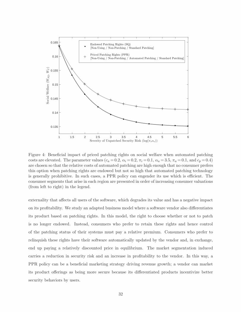
1 1.5 2 2.5 3 3.5 4 4.5 5 5.5 6Severity of Unpatched Security Risk (log(πsαs))

0.135

0.14

0.145

0.15

0.155

0.16

0.165

Social

Welfare

(WSQ,W

P)

Endowed Patching Rights (SQ)[Non-Using / Non-Patching / Standard Patching]

Priced Patching Rights (PPR)[Non-Using / Non-Patching / Automated Patching / Standard Patching]

Figure 4: Beneficial impact of priced patching rights on social welfare when automated patchingcosts are elevated. The parameter values (ca =0.2, αi=0.2, πi=0.1, αa=3.5, πa=0.1, and cp =0.4)are chosen so that the relative costs of automated patching are high enough that no consumer prefersthis option when patching rights are endowed but not so high that automated patching technologyis generally prohibitive. In such cases, a PPR policy can engender its use which is efficient. Theconsumer segments that arise in each region are presented in order of increasing consumer valuations(from left to right) in the legend.

externality that affects all users of the software, which degrades its value and has a negative impact

on its profitability. We study an adapted business model where a software vendor also differentiates

its product based on patching rights. In this model, the right to choose whether or not to patch

is no longer endowed. Instead, consumers who prefer to retain these rights and hence control

of the patching status of their systems must pay a relative premium. Consumers who prefer to

relinquish these rights have their software automatically updated by the vendor and, in exchange,

end up paying a relatively discounted price in equilibrium. The market segmentation induced

carries a reduction in security risk and an increase in profitability to the vendor. In this way, a

PPR policy can be a beneficial marketing strategy driving revenue growth; a vendor can market

its product offerings as being more secure because its differentiated products incentivize better

security behaviors by users.

32

A PPR policy is a very effective way to improve software security. The size of unpatched users

decreases in equilibrium under PPR which, in turn, tends to lead to a decrease in losses associated

with security attacks on systems running the software. In some cases, the firm may raise both the

price of the premium version with patching rights and the price of the “discounted” version without

patching rights relative to the optimal price offered under the status quo. This demonstrates how

a software firm can extract value from a combination of improved automated patching technology

and a pricing strategy that incentivizes better security outcomes that are valued by consumers. A

PPR policy can negatively affect social welfare when usage in the market significantly contracts,

but in many cases it increases welfare as a result of the lower resulting security risk.

Our study is a simplification of a software vendor’s versioning strategy which, more practically,

can involve managing numerous quality-differentiated versions, bundled security/feature updates,

interim update versus major release cycles, and planned obsolescence. The intent of our simplifica-

tion is to put a spotlight on the value of PPR as a tool that provides incentives for lower-valuation

users to engage in better behaviors that help reduce the effective security externality. Even in

the complex settings that exist in the software industry, the ideas and insights stemming from

our work can improve software outcomes if, however implemented, lower-valuation users ultimately

select versions that remain up to date with security patches. In the software industry, vendors

have taken greater actions to ensure that versions of their products stay updated (e.g., the offering

of automatic updates, configuring of default options to turn automatic updates on, and even ver-

sions of software which forcibly update). Our work helps clarify the impact of actions that aim to

incentivize lower-valuation users to forgo patching rights.

Despite the benefits, there are many frictions associated with the essence of a PPR policy

which can cause vendors to resist adoption. First, by forcibly updating users who choose to forgo

patching rights for discounted versions of the software, the vendor is exposing these users to system

instability risk. While these losses are internal to the model and part of the trade-off evaluated

by users, vendors may shy away from additional exposure to liability. Second, whenever there is

a patch that leads to severe instability, vendors may likely receive backlash from consumers and

incur damage to their reputation. In this regard, any vendor strategy that eliminates patching

rights from a market segment may go hand-in-hand with investments in patch quality. In that

many software vendors have been providing the option of automatic updates for years now, they

have made significant progress on patch stability. In order for more vendors to consider adoption of

a PPR policy (or practical variants), assurance of patch stability will be critical because the policy

33

leaves the targeted consumer tier with little recourse.

5.1 Alternative Models and Application Domains of PPR

The manner in which software is licensed and updated is constantly changing due to technology

disruptions and the developing needs of consumers. While there is some diversity in observed

licensing strategies in the software industry, the current work focuses on an important and large

class of software products where patches are predominantly made freely available to users who then

make decisions whether or not to install them. This class includes versions of software products

from an extensive list of top vendors such as Microsoft, Oracle, Symantec, VMware, and IBM.13

We discuss both alternative models to PPR and other potential application domains of PPR,

highlighting in the latter whether PPR-type policies are likely to be effective in the domain of

interest.

Some producers make software source code available for free and build revenue models around

service and support (e.g., Red Hat Enterprise Linux, Elasticsearch, and Oracle Java). In this open-

source domain, when software is made available for free, developers have no obligation to provide

patches. One approach that has been observed is the offering of patches only to paying customers

who have contracted for support. This alternative model involves charging for patches. Oracle

has done this by offering the patches only for paying customers of its freely available open-source

Java software (Krill 2015). We examine how this strategy compares to PPR. First, it is important

to understand what happens when an OSS developer does not provide patches to its users. In

such a setting, a consumer’s options can include: (i) use the software for free and be unpatched,

risking security attacks, (ii) not use the software, and (iii) leverage the open-source nature of the

software to self-patch.14 Because the software has zero price, if the effective security risk is low,

all consumers will use the software and obtain positive surplus in equilibrium. On the other hand,

if the effective security risk exceeds a certain bound, then users can only enter until the size of

the unpatched population reaches a critical size upon which dependent risk wipes out all surplus

derived from any unpatched use of the software.

In such a context, the offering of a patch alone will significantly improve welfare. Patches

enable high-valuation users to shield themselves from risk, which in turn can reduce the security

13Examples of specific software products that can be installed on-premises and maintained by users include Mi-crosoft Windows, Microsoft Office, Microsoft SQL Server, Oracle Database, Oracle WebLogic Server, Norton An-tivirus, Symantec Endpoint Protection, VMware Workstation, and IBM WebSphere.

14Only a select group of users might have the capability to self-patch.

34

externality that decays the surplus of users who choose to remain unpatched. Suppose a vendor

offers patches only to those who agree to pay for them as part of a support package. This provides

users the additional usage option to pay for patches. Examining conditions analogous to Section 4.2,

the equilibrium consumer market structure will be characterized by both patched and unpatched

usage. Because high-valuation consumers can now patch and protect themselves from attack, social

surplus will increase in equilibrium in comparison to the case where it is mostly wiped out in the

presence of high risk and patch unavailability.

One can compare our PPR policy to this alternative model where an OSS developer prices

the patch itself. A PPR policy will tend to dominate this alternative model both in terms of

profitability and in terms of welfare. It is straightforward to see why it is more profitable. Because

a PPR policy charges premia for both unpatched and standard patched usage and even a positive

price for automatic patched usage, it generates a lot of direct revenue. The alternative model

requires all the revenues to come from higher-valuation users who need to be willing to pay for

access to patches. By giving the software away for free, one’s revenue model typically hinges on the

creation of positive network effects and leveraging those to create higher willingness-to-pay within

the higher-value segment. However, this alternative model has payment tied to security patches,

which means that the higher value segment will only be willing to pay for patches if the security

risk is large. This suggests that risk stemming from expanded usage is necessarily required, but

that lies in stark contrast to any sort of positive network effects strategy. These opposing effects

handicap this model in comparison to the PPR policy being advocated here.

In terms of social welfare, this alternative model suffers relative disadvantages dependent upon

the region of concern. If automated costs are comparable to standard patching costs, a PPR strategy

expands overall usage relative to the status quo by incentivizing more users to select automated

patching. This usage expansion is also much larger than can be expected under the alternative

model because in that case users have fewer options and cannot readily shield risk without paying a

premium – this lies in contrast to the PPR strategy where unpatched users are provided incentives

instead to reduce risk. If automated patching costs are large and it becomes difficult to incentivize

automated patching, then the alternative model can in fact generate greater usage than under a

PPR policy. However, expanded usage of the free product increases the externality to the point

where unpatched users gain no surplus in the alternative model. Therefore, even in this case, the

PPR policy achieves higher welfare with a smaller user segment, where they derive positive surplus

from the reduced security risk.

35

Even for OSS providers who are not charging for patches, a PPR policy can be a valuable option.

In particular, OSS providers who are already employing other monetization strategies can easily

implement the essence of a PPR policy and benefit via improved security and revenues. On the

other hand, OSS providers who are not currently differentiating their offerings and whose mission is

perhaps more squarely centered on public good are not likely to be good candidates for PPR. Such

providers may find both the concept of giving up rights and charging for software to be inconsistent

with their mission.

Next, there are many producers who offer subscriptions for access to SaaS (e.g., Salesforce

CRM, Workday, and NetSuite). In this domain, a vendor manages the patching process directly so

that consumers no longer make a decision about whether or not to patch. However, this certainly

comes at a cost to the provider, which ultimately gets reflected in the price consumers pay. SaaS

software tends to run on a fairly limited set of servers under the control of the vendor, whereas

in the on-premises model the number of systems running software tends to be much larger with

decision-making rights being distributed. In the case of on-premises software studied in our model,

it is often the case that patchable vulnerabilities are exploited. This occurs because malicious

individuals study the vulnerability that has been addressed in the patch, and then exploit the

same vulnerability hoping to successfully attack some subset of users who remain in an unpatched

state. In the case of SaaS, the approach to finding vulnerabilities differs significantly as both the

software as well as patches to the software remain internal to the vendor. Malicious agents must

find vulnerabilities in the interface to the SaaS product itself. On the consumer side, it can be the

case that companies (particularly small and medium-sized businesses) fully commit to the cloud

as part of their IT strategies, which may introduce correlated risks on cloud platforms and make

it difficult to analyze a PPR strategy in an context where a vendor additionally offers both on-

premises and SaaS alternatives. Because of the many differences in characteristics that surface when

comparing SaaS to on-premises software, a PPR policy does not fit the SaaS domain very well.

However, studying the role of PPR under the additional complexity of mixed offerings (SaaS and

on-premises) is potentially a fruitful direction for future research because of the distinct security

risks associated with the different licensing models (August et al. 2014)

the service. Comparing this model to pricing patching rights, we find that when the service

quality is high enough, then the SaaS model outperforms pricing patching rights both in terms of

profitability and in terms of welfare. This is clear since consumers incur no patching losses to be

shielded from attack, which then allows the vendor to extract more surplus and be more profitable.

36

On the other extreme, when γ is low enough, then the software is of poor quality so that the SaaS

model is outperformed by pricing patching rights. When γ is in an intermediate range, then the

SaaS model outperforms pricing patching rights in terms of welfare while pricing patching rights is

more profitable. Under high security risk, the equilibrium market size under a priced patching rights

strategy in which all market segments are present (either 0<vb <va<vp< 1 or 0<va<vb <vp< 1)

would be larger than the total market size under the SaaS model. However, consumers incur losses

through either patching or bearing security risks that ultimately make welfare worse off in aggregate.

Software producers have long shielded themselves from liability using well-crafted license agree-

ments. However, the increasing breadth of software use in riskier operating environments (including

the critical infrastructure, biomedical products, and automobiles) comes with increased exposure

to strict liability. In particular, liability concerns come to the forefront in software contexts where

system failure can lead to safety or health hazards. For example, researchers have demonstrated the

ability to hack into automotive systems and hijack control over brakes and steering from drivers;

vulnerabilities such as these can be utilized to cause physical harm to citizens (Greenberg 2015). In

application domains with this property, a PPR policy may be inappropriate. In our model, these

settings would be characterized as having high automated patching risk (i.e., a large πaαa param-

eter), in which case a PPR strategy is shown to be weakly dominated. Intuitively, manufacturers

would likely not agree to have embedded software on products such as pacemakers automatically

updated. In the presence of strict liability, assurance of quality takes precedence.

Many issues tackled in this paper will become increasingly salient as the Internet of things

(IoT) comes of age. With IoT, the explosion of interconnected devices will be accompanied by both

increased vulnerabilities and increased threats as malicious actors evolve to exploit new possibilities.

The standard patching processes employed by organizations will face significant challenges with the

scale of device growth and their complex interactions. IoT’s scale will require a greater level of

automation in patch management. The extent and type of human interaction taking place with

software that drives servers, laptops, tablets and phones is fundamentally different than that with

the embedded software that drives IoT devices. This, in turn, may necessitate greater sophistication

with the automated management of IoT devices. In this landscape, IoT presents as both a challenge

and opportunity for security interventions like a PPR policy. For PPR to be effective in this domain,

automated patching technology must first improve and attain a service level where minimal failure

rates are observed. Until then, it may be premature to consider a PPR policy for IoT devices.

37

5.2 Concluding Remarks

Standard patching costs (cp) may increase with factors such as the relative size of a user firm,

for instance, depending on the number of servers on which they run the software product. A

primary driver is that a larger number of users require a higher number of servers likely in different

environments and configurations on which to patch the software, driving up the patching costs

proportional to the number of servers. Our results however continue to hold with consideration

of this dimension: In our model, each host can be considered to be a single server and a large

corporation can be thought to have a number of different servers. Our analysis is unaffected

provided each decision maker owns at most countably many hosts. It may also be the case that

two organizations conducting the same tasks associated with a rigorous, standard patching process

would have some variation in the costs incurred. For example, there may be some variation around

one thousand dollars per server. Having some variation in this regard will not qualitatively change

any of our results for two reasons. First, given the nature of the tasks being performed, there will

always be a primary, valuation-independent component of these costs which is currently captured.

Second, inclusion of a valuation-dependent component will ultimately be swamped by the valuation-

dependent losses that are currently present in the model. In particular, in our model, both losses

due to system instability and losses due to security attacks are valuation-dependent. Importantly,

both of these losses are much more strongly associated with valuation than the residual component

of patching costs, which limits its impact.

We focus on the case where a software vendor releases and immediately applies automatic

updates to all systems that have opted in to this form of patching. One interesting extension would

be to explore the dynamics of automated patch deployment. In particular, some vendors may prefer

to slowly roll out an automated update to subsets of systems that have opted-in and subsequently

ramp up roll out as the vendor builds confidence in the quality of its patch (as measured by

monitoring of systems that have been updated). Another related extension would be to explore

how a vendor’s investment in patch quality interacts with this dynamic deployment strategy.

Our study constructs a model of a monopolist software vendor to study PPR. In practice,

essentially no sector is monopolistic and there is some competition in any industry and market.

However, as long as the firms in the market have some market power (which is true in almost every

industry and market, and certainly for the software industry), a monopolistic model captures most

of the insights that would come out from the intended arguments in an oligopoly model of the same

38

situation in a much clearer and transparent way. In general, increased competition will negatively

affect firm profits and likewise the profitability of PPR, and studying competition-related questions

would be an interesting direction for future research.

Under the framework of a PPR policy, the consumers who pay a premium to retain patching

rights need no additional monitoring by the proprietary vendor or OSS provider to examine patching

status. However, consumers who benefit financially in exchange for these rights must have their

systems automatically updated per the contract. This requires a careful implementation that

entails the monitoring of systems. First, the updating of systems need not be in full control by

the vendor nor instantaneous to derive the benefits of this policy. For example, consumers can be

given a time window to apply patches before they are forcefully installed. This gives users some

leeway operationally. Second, vendors can modify the implementation of PPR to the environment

in which they reside. For example, mobile application developers could give a discount to users

willing to automatically update their software, and even give a slightly greater discount to those

who are willing to receive those updates immediately through their mobile data plan. Lastly, a

user can always disconnect her system from the Internet to avoid the deployment of automated

security updates. In this case, although the patches are not installed, the externality imposed by

this unpatched system would also be partially reduced.

Acknowledgments

The authors thank Anandhi Bharadwaj (the department editor), the associate editor, and the

anonymous reviewers for their valuable comments and suggestions throughout the review process.

The authors also thank the participants at the Workshop on the Economics of Information Secu-

rity 2016, Conference on Information Systems and Technology 2016, INFORMS 2016, Theory in

Economics of Information Systems 2018, as well as the participants in research seminars at Ko-

rea University, University of Utah, University of Minnesota, and University of Calgary for their

helpful discussions. This material is based upon work partially supported by the National Science

Foundation under Grant No. CNS-0954234.

References

Adams, W. J. and J. L. Yellen (1976). Commodity bundling and the burden of monopoly. TheQuarterly Journal of Economics 90 (3), 475–498.

Arora, A., R. Telang, and H. Xu (2008). Optimal policy for software vulnerability disclosure.Management Science 54 (4), 642–656.

39

August, T., R. August, and H. Shin (2014). Designing user incentives for cybersecurity. Commu-nications of the ACM 57 (11), 43–46.

August, T., D. Dao, and H. Shin (2015). Optimal timing of sequential distribution: The impactof congestion externalities and day-and-date strategies. Marketing Science 34 (5), 755–774.

August, T., M. F. Niculescu, and H. Shin (2014). Cloud implications on software network struc-ture and security risks. Information Systems Research 25 (3), 489–510.

August, T. and T. I. Tunca (2006). Network software security and user incentives. ManagementScience 52 (11), 1703–1720.

August, T. and T. I. Tunca (2011). Who should be responsible for software security? A com-parative analysis of liability policies in network environments. Management Science 57 (5),934–959.

Bakos, Y. and E. Brynjolfsson (1999). Bundling information goods: Pricing, profits, and effi-ciency. Management Science 45 (12), 1613–1630.

Beattie, S., S. Arnold, C. Cowan, P. Wagle, and C. Wright (2002, November). Timing theapplication of security patches for optimal uptime. Proceedings of LISA ’02: Sixteenth SystemsAdministration Conference, 233–242.

Beattie, S., S. Arnold, C. Cowan, P. Wagle, C. Wright, and A. Shostack (2002). Timing theapplication of security patches for optimal uptime. Proceedings of the 16th USENIX conferenceon system administration, 233–242.

Beres, Y. and J. Griffin (2009). Optimizing network patching policy decisions. HP Laboratories.

Berr, J. (2017). ”wannacry” ransomware attack losses could reach $4 billion. CBS News Mon-eyWatch. Available at https://www.cbsnews.com/news/wannacry-ransomware-attacks-

wannacry-virus-losses/.

Bhargava, H. K. (2013). Mixed bundling of two independently valued goods. Management Sci-ence 59 (9), 2170–2185.

Bhargava, H. K. and V. Choudhary (2001). Information goods and vertical differentiation. Jour-nal of Management Information Systems 18 (2), 89–106.

Bhargava, H. K. and V. Choudhary (2008). Research note: When is versioning optimal forinformation goods? Management Science 54 (5), 1029–1035.

Bloor, B. (2003). The patch problem: It’s costing your business real dollars. http://www.

netsense.info/downloads/PatchProblemReport_BaroudiBloor.pdf.

Brillinger, D. (1966). The analyticity of the roots of a polynomial as functions of the coefficients.Mathematics Magazine 39 (3), 145–147.

Brito, D. L., E. Sheshinski, and M. D. Intriligator (1991, June). Externalities and compulsoryvaccinations. J. Public Econ. 45 (1), 69–90.

Cavusoglu, H., H. Cavusoglu, and S. Raghunathan (2007). Efficiency of vulnerability disclosuremechanisms to disseminate vulnerability knowledge. IEEE Transactions on Software Engi-neering 33 (3), 171–185.

Cavusoglu, H., H. Cavusoglu, and J. Zhang (2008). Security patch management: Share theburden or share the damage? Management Science 54 (4), 657–670.

CCIRC (2014, October). Top 4 strategies to mitigate targeted cyber intrusions. Available athttp://www.publicsafety.gc.ca/cnt/ntnl-scrt/cbr-scrt/tp-strtgs-eng.aspx.

40

Chen, F. (2001). Market segmentation, advanced demand information, and supply chain perfor-mance. Manufacturing & Service Operations Management 3 (1), 53–67.

Choi, J. P., C. Fershtman, and N. Gandal (2010). Network security: Vulnerabilities and disclosurepolicy. Journal of Industrial Economics 58 (4), 868–894.

Cormen, T. H., C. E. Leiserson, R. L. Rivest, and C. Stein (2009, July). Introduction to Algo-rithms (3 ed.). U.S.A.: The MIT Press.

Debo, L. G., L. B. Toktay, and L. N. V. Wassenhove (2005). Market segmentation and producttechnology selection for remanufacturable products. Management Science 51 (8), 1193–1205.

Desai, P. S. (2001). Quality segmentation in spatial markets: When does cannibalization affectproduct line design? Marketing Science 20 (3), 265–283.

Dey, D., A. Lahiri, and G. Zhang (2015). Optimal policies for security patch management. Journalon Computing 27 (3), 462–477.

Eckalbar, J. C. (2010). Closed-form solutions to bundling problems. Journal of Economics &Management Strategy 19 (2), 513–544.

Fitzgerald, D. (2015, May). Level 3 tries to waylay hackers. The Wall Street Journal.

Forbath, T., P. Kalaher, and T. O’Grady (2005). The total cost of security patch management.Wipro Technologies, Ltd..

Gabszewicz, J. J., A. Shaked, J. Sutton, and J.-F. Thisse (1986). Segmenting the market: Themonopolist’s optimal product mix. Journal of Economic Theory 39 (2), 273–289.

Greenberg, A. (2015, July). Hackers remotely kill a jeep on the highway - with me in it. WIRED.

Greenberg, A. (2017, May). The wannacry ransomware hackers made some real amateur mistakes.Fortune.

Gupta, A. and D. Zhdanov (2012). Growth and sustainability of managed security services net-works: An economic perspective. MIS Quarterly 36 (4), 1109–1130.

Hick, M. (2012, June). Apple acknowledges Flashback malware with update. Huffington PostUK.

Higgins, S. (2017). Ethereum client update issue costs cryptocurrency exchange $14 million.Available at https://www.coindesk.com/ethereum-client-exchange-14-million/.

HP Security Research (2015, February). Hp cyber risk report 2015. Available at http://www8.hp.com/us/en/software-solutions/cyber-risk-report-security-vulnerability/.

Ingram, M. (2015, July). Mobile botnets are costing advertisers $1 billion in ad fraud, studyshows. Fortune.

Johnson, J. P. and D. P. Myatt (2003, Jun). Multiproduct quality competition: Fighting brandsand product line pruning. The American Economic Review 93 (3), 748–774.

Kannan, K., M. S. Rahman, and M. Tawarmalani (2013, Jan). Economic and policy implicationsof restricted patch distribution. Working paper, Purdue University and University of Calgary.

Krill, P. (2015, April). Oracle to end publicly available security fixes for java 7 this month.InfoWorld.

Laffont, J.-J. and J. Tirole (1988). The dynamics of incentive contracts. Econometrica 56 (5),1153–1175.

41

Lahiri, A. (2012). Revisiting the incentive to tolerate illegal distribution of software products.Decision Support Systems 53 (2), 357–367.

Levchenko, K., A. Pitsillidis, N. Chachra, B. Enright, M. Felegyhazi, C. Grier, T. Halvorson,C. Kanich, C. Kreibich, H. Liu, D. McCoy, N. Weaver, V. Paxson, G. M. Voelker, and S. Sav-age (2011). Click trajectories: End-to-end analysis of the spam value chain. In Proceedingsof the 2011 IEEE Symposium on Security and Privacy, SP ’11, Washington, DC, USA, pp.431–446. IEEE Computer Society.

Li, L., R. D. McKelvey, and T. Page (1987). Optimal research for Cournot oligopolists. Journalof Economic Theory 42 (1), 140–166.

Lohr, S. and L. Alderman (2017, May). The fallout from a global cyberattack: ‘a battle werefighting every day’. The New York Times.

MacLeod, W. B. and J. M. Malcomson (1993). Investments, holdup, and the form of marketcontracts. American Economic Review 83 (4), 811–837.

Maskin, E. and J. Riley (1984). Monopoly with incomplete information. RAND Journal of Eco-nomics 15 (2), 171–196.

McAfee, R. P., J. McMillan, and M. D. Whinston (1989, May). Multiproduct monopoly, com-modity bundling, and correlation of values. The Quarterly Journal of Economics 104 (2),371–383.

Microsoft (2017a). New ransomware, old techniques: Petya adds worm capabilities. MicrosoftMalware Protection Blog Post. Available at https://blogs.technet.microsoft.com/mmpc/2017/06/27/new-ransomware-old-techniques-petya-adds-worm-capabilities/.

Microsoft (2017b). Wannacrypt ransomware worm targets out-of-date systems. Microsoft Mal-ware Protection Blog Post. Available at https://blogs.technet.microsoft.com/mmpc/

2017/05/12/wannacrypt-ransomware-worm-targets-out-of-date-systems/.

Miller, P. D. (2006). Applied Asymptotic Analysis, Volume 75 of Graduate Studies in Mathemat-ics. Providence, Rhode Island: American Mathematical Society.

Moorthy, K. S. (1984). Market segmentation, self-selection, and product line design. MarketingScience 3 (4), 288–307.

Moorthy, K. S. and I. Png (1992). Market segmentation, cannibalization, and the timing ofproduct introductions. Management Science 38 (3), 345–359.

Muller, H. M. (2000). Asymptotic efficiency in dynamic principal-agent problems. Journal ofEconomic Theory 91, 292–301.

Mussa, M. and S. Rosen (1978). Monopoly and product quality. Journal of Economic The-ory 18 (2), 301–317.

Netessine, S. and T. A. Taylor (2007). Product line design and production technology. MarketingScience 26 (1), 101–117.

OPSWAT (2014, October). Antivirus and operating system report. Available at https://www.opswat.com/resources/reports/antivirus-october-2014.

Pei, P. P.-E., D. Simchi-Levi, and T. I. Tunca (2011). Sourcing flexibility, spot trading, andprocurement contract structure. Operations Research 59 (3), 578–601.

Pesendorfer, W. and J. M. Swinkels (2000). Efficiency and information aggregation in auctions.American Economic Review 90 (3), 499–525.

42

Png, I. P. and Q. Wang (2009). Information security: Facilitating user precautions vis-a-visenforcement against attackers. Journal of Management Information Systems 26 (2), 97–121.

Prasad, A., R. Venkatesh, and V. Mahajan (2010). Optimal bundling of technological productswith network externality. Management Science 56 (12), 2224–2236.

Ransbotham, S., S. Mitra, and J. Ramsey (2012). Are markets for vulnerabilities effective? MISQuarterly 36 (1), 43–64.

Sarkar, D. and B. LeBlanc (2018). Announcing windows 10 insider preview build 17134 for fast.Windows Blog Post. Available at https://blogs.windows.com/windowsexperience/2018/04/16/announcing-windows-10-insider-preview-build-17134-for-fast/.

Schmalensee, R. (1984, January). Gaussian demand and commodity bundling. The Journal ofBusiness 57 (1), S211–S230.

Stremersch, S. and G. J. Tellis (2002, January). Strategic bundling of products and prices: Anew synthesis for marketing. Journal of Marketing 66, 55–72.

Thomson, I. (2017). Notpetya ransomware attack cost us $300m shipping giant Maersk. The Reg-ister. Available at https://www.theregister.co.uk/2017/08/16/notpetya_ransomware_

attack_cost_us_300m_says_shipping_giant_maersk/.

Tunca, T. I. and S. A. Zenios (2006). Supply auctions and relational contracts for procurement.M&SOM 8 (1), 43–67.

US-CERT (2015). Top 30 targeted high risk vulnerabilities. US-CERT Alert (TA15-119A). Avail-able at https://www.us-cert.gov/ncas/alerts/TA15-119A.

Venkatesh, R. and W. A. Kamakura (2003). Optimal bundling and pricing under a monopoly:Contrasting complements and substitutes from independently valued products. The Journalof Business 76 (2), 211–231.

Villas-Boas, J. M. (2004). Communication strategies and product line design. Marketing Sci-ence 23 (3), 304–316.

Villas-Boas, J. M. (2009). Product variety and endogenous pricing with evaluation costs. Man-agement Science 55 (8), 1338–1346.

Westervelt, R. (2014). Microsoft fixes faulty windows security patch that was causing bluescreen of death for some. Available at http://www.crn.com/news/security/300073858/

microsoft-fixes-faulty-windows-security-patch-that-was-causing-blue-screen-

of-death-for-some.htm.

43

Online Supplement for

Market Segmentation and Software Security:Pricing Patching Rights

Terrence August, Duy Dao, and Kihoon Kim

(Rady School of Management, Haskayne School of Business,and Korea University Business School)

Proofs of Propositions

A High πiαi

1 Status Quo

Lemma A.1 When πiαi > 1, under the status quo, i.e., δ=1, the complete threshold characteri-

zation of the consumer market equilibrium is as follows:

(I) (0 < va < 1), where va = p+ca1−πaαa

:

(A) p+ ca + πaαa < 1

(B) cp ≥ ca + πaαa

(C) cp ≥ ca+pπaαa

1−πaαa

(II) (0 < va < vp < 1), where va = p+ca1−πaαa

and vp =cp−caπaαa

:

(A) cp < ca + πaαa

(B) cp >ca+pπaαa

1−πaαa

(III) (0 < vp < 1), where vp = p+ cp:

(A) cp + p < 1

(B) cp ≤ ca+pπaαa

1−πaαa

Proof of Lemma A.1: This is a sub-case in the proof of Lemma A.2, by setting δ = 1. �

Proof of Lemma 2: We prove that if πiαi> 1 and δ=1 (i.e., when patching rights are not

priced), then if cp − πaαa < ca < 1− πaαa − (1− cp)√1− πaαa, we have that

p∗=1− πaαa − ca

2, (A.1)

A.1

and σ∗ is characterized by 0<va<vp< 1 such that the lower tier of users prefers automated patch-

ing. On the other hand, if ca ≥ 1− πaαa − (1− cp)√1− πaαa, then

p∗=1− cp

2, (A.2)

and σ∗ is characterized by 0<vp< 1 such that there is no user of automated patching in equilibrium.

Suppose 0 < va < 1 is induced. Then the profit function is ΠI(p) = p(1 − va). Using Lemma

A.1, we have that va = p+ca1−πaαa

. The optimal price is found to be p∗1 = 12 (1− ca − πaαa) with the

corresponding profit Π∗I =

(1−ca−πaαa)2

4(1−πaαa).

Similarly, suppose instead that 0 < va < vp < 1 is induced. Then the profit function is

ΠII(p) = p(1 − va). Using Lemma A.1, we have that va = p+ca1−πaαa

. Again, the optimal price is

found to be p∗2 =12 (1− ca − πaαa) with the corresponding profit Π∗

II =(1−ca−πaαa)2

4(1−πaαa).

Lastly, suppose that 0 < vp < 1 is induced. Then the profit function is ΠIII(p) = p(1 − vp).

Using Lemma A.1, we have that vp = cp + p. Now, the optimal price is found to be p∗3 =1−cp2 with

the corresponding profit Π∗III =

(1−cp)2

4 .

We next find conditions under which the maximizing price for each case indeed induces that

market structure. For 0 < va < 1, we need the set of conditions for Case (I) in Lemma A.1 to hold

for p∗1. To satisfy the first condition, we need p+ca+πaαa < 1 for p = p∗1 =12 (1− ca − πaαa). This

simplifies to ca+πaαa < 1, which is a preliminary model assumption. Then we need cp ≥ ca+pπaαa

1−πaαa

to hold for p = p∗1 as well, which simplifies to ca ≤ (2cp−πaαa)(1−πaαa)2−πaαa

. We also needed the condition

ca ≤ cp − πaαa for this case to hold. Since(2cp−πaαa)(1−πaαa)

2−πaαa> cp − πaαa follows from 0 < cp < 1

and 0 < πaαa < 1, then the condition under which p∗1 would induce 0 < va < 1 is ca ≤ cp − πaαa.

Similarly, for Case (II), the condition under which p∗2 would induce 0 < va < vp < 1 is cp−πaαa <

ca <(2cp−πaαa)(1−πaαa)

2−πaαa. And lastly, for Case (III), the condition under which p∗3 would induce

0 < vp < 1 is ca ≥ cp − 12 (1 + cp) πaαa. Note that cp − 1

2 (1 + cp) πaαa <(2cp−πaαa)(1−πaαa)

2−πaαa, so that

when cp − 12 (1 + cp)πaαa < ca <

(2cp−πaαa)(1−πaαa)2−πaαa

, we’ll need to compare Π∗II and Π∗

III .

Next, we find the conditions under which the maximal profits of each case dominate the other

cases. In particular, when ca < cp − 12 (1 + cp)πaαa, then Π∗

I = Π∗II > Π∗

III . Since cp − πaαa <

cp− 12 (1 + cp) πaαa from cp < 1, this implies that 0 < va < 1 will be the resulting consumer market

structure for ca ≤ cp−πaαa. Also, 0 < va < vp < 1 will be the resulting consumer market structure

for cp − πaαa < ca < cp − 12 (1 + cp) πaαa.

Also, for ca >(2cp−πaαa)(1−πaαa)

2−πaαa, we have that Π∗

III > Π∗II , so that 0 < vp < 1 will be the

resulting market structure when ca >(2cp−πaαa)(1−πaαa)

2−πaαa.

In between cp − 12 (1 + cp)πaαa < ca <

(2cp−πaαa)(1−πaαa)2−πaαa

, we find the conditions under which

Π∗II dominates Π∗

III . Comparing the profits, we find that Π∗II ≥ Π∗

III when ca ≤ 1 − πaαa − (1 −cp)√

(1− πaαa). Then we note that cp − 12 (1 + cp)πaαa < 1 − πaαa − (1 − cp)

√(1− πaαa) <

(2cp−πaαa)(1−πaαa)2−πaαa

always holds, so that the resulting market structure when cp − πaαa < ca <

1 − πaαa − (1 − cp)√1− πaαa is 0 < va < vp < 1, and the resulting market structure when

ca ≥ 1− πaαa − (1− cp)√1− πaαa is 0 < vp < 1. �

A.2

2 Pricing Patching Rights

Lemma A.2 When πiαi > 1, under PPR, the complete threshold characterization of the consumer

market equilibrium is as follows:

(I) (0 < va < 1), where va = δp+ca1−πaαa

:

(A) δp+ ca + πaαa < 1

(B) cp + (1− δ)p ≥ ca + πaαa

(C) cp ≥ ca+p(πaαa−(1−δ))1−πaαa

(II) (0 < va < vp < 1), where va = δp+ca1−πaαa

and vp =(1−δ)p+cp−ca

πaαa:

(A) cp + (1− δ)p < ca + πaαa

(B) cp >ca+p(πaαa−(1−δ))

1−πaαa

(III) (0 < vp < 1), where vp = p+ cp:

(A) cp + p < 1

(B) cp ≤ ca+p(πaαa−(1−δ))1−πaαa

Proof of Lemma A.2: First, we establish the general threshold-type equilibrium structure. The

proof of this is a sub-case of the argument in Lemma A.4, with the size of the unpatched user

population u = 0 since πiαi > 1. This establishes the threshold-type consumer market equilibrium

structure.

Next, we characterize in more detail each outcome that can arise in equilibrium, as well as the

corresponding parameter regions. For Case (I), in which all consumers who purchase choose the

automated patching option, i.e., 0 < va < 1, based on the threshold-type equilibrium structure,

we have u = 0. For this market structure to be an equilibrium, we need va > 0, va < 1, the

consumer v = 1 weakly preferring (B,AP ) over (B,P ), and the consumer v = va weakly preferring

(NB,NP ) over (B,P ).

The condition va > 0 is satisfied by our assumption that πaαa < 1, since va = δp+ca1−πaαa

. Then for

va < 1, we need δp+ ca +πaαa < 1. For v = 1 to weakly prefer (B,AP ) over (B,P ), it needs to be

the case that v− δp− ca−πaαav ≥ v−p− cp for v = 1. This simplifies to cp+(1− δ)p ≥ ca+πaαa.

For v = va to weakly prefer (NB,NP ) over (B,P ), it needs to be the case that 0 ≥ v − p− cp for

v = va = δp+ca1−πaαa

. This simplifies to cp ≥ ca+p(πaαa−(1−δ))1−πaαa

.

Next, for case (II), in which the top tier purchases (B,P ) but the lower tier of consumers

purchase (B,AP ), i.e., 0 < va < vp < 1, we have va = δp+ca1−πaαa

and vp =(1−δ)p+cp−ca

πaαa. Following

the same steps as before, we find the corresponding conditions for which case (II) arises. For this

case to arise, we need va > 0, vp > va, and vp < 1. Again, va > 0 is satisfied under πaαa < 1,

one of the preliminary assumptions of the model. To have vp > va, we need(1−δ)p+cp−ca

πaαa> δp+ca

1−πaαa.

This simplifies to cp > ca+p(πaαa−(1−δ))1−πaαa

. Lastly, to have vp < 1, we need(1−δ)p+cp−ca

πaαa< 1. This

simplifies to cp + (1− δ)p < ca + πaαa.

A.3

Lastly, for case (III), in which consumers who purchase are all standard patching, choosing

(B,P ), vp = p + cp. For this case to be an equilibrium, we need vp > 0, vp < 1, v = vp preferring

(NB,NP ) over (B,AP ), and v = vp preferring (B,P ) over (B,AP ). The condition vp > 0 is

satisfied. For vp < 1, we need the condition cp+p < 1. For v = vp to prefer (NB,NP ) over (B,AP ),

we need 0 ≥ v− δp− ca−πaαav for v = vp = cp+p. This becomes cp+(1− δ)p ≤ ca+(cp+p)πaαa.

Lastly, for v = vp to prefer (B,P ) over (B,AP ), we need v − p − cp ≥ v − δp − ca − πaαav for

v = vp = cp + p. This also simplifies to cp ≤ ca+p(πaαa−(1−δ))1−πaαa

. This concludes the proof of the

consumer market equilibrium for the PPR case when πiαi > 1. �

Proof of Lemma 3: We prove that if πiαi > 1 and patching rights are priced by the vendor,

then if cp − πaαa < ca ≤ cp(1− πaαa), we have

p∗ =1− cp

2, (A.3)

δ∗ =1− ca − πaαa

1− cp, (A.4)

and σ∗ is characterized by 0<va<vp< 1 such that the lower tier of users prefers automated patch-

ing. On the other hand, if ca > cp(1− πaαa), then

p∗=1− cp

2, (A.5)

and σ∗ is characterized by 0<vp< 1 such that there is no user of automated patching in equilibrium.

Suppose 0 < va < 1 is induced. Then the profit function is ΠI(p, δ) = δp(1− va). Using Lemma

A.2, we have that va = δp+ca1−πaαa

. Similar to the status quo case, the optimal price and discount

satisfies δ∗1p∗1 =1−ca−πaαa

2 with the corresponding profit Π∗I =

(1−ca−πaαa)2

4(1−πaαa). Notice in this case that

there is not a unique maximizer, and in fact, the optimal (p∗, δ∗) traces out an isoprofit curve.

Next, suppose that 0 < va < vp < 1 is induced. Then the profit function is ΠII(p, δ) = p(1 −vp)+δp(vp−va). Using Lemma A.2, we have that va = δp+ca

1−πaαaand vp =

(1−δ)p+cp−caπaαa

. From the first-

order condition for p, we have p∗2(δ) =(1−πaαa)(−cp(1−δ)+πaαa)−ca(1−δ−πaαa))

2((1−δ)2−πaαa(1−2δ))with the second-order

condition satisfied. Then maximizing ΠII(p∗2(δ), δ) with respect to δ, we find that δ∗2 = 1−ca−πaαa

1−cp,

and so p∗2 = p∗2(δ∗2) =

1−cp2 . The corresponding profit is ΠII =

14

(1− 2cp +

(ca−cp)2

πaαa+ c2a

1−πaαa

).

Lastly, suppose that 0 < vp < 1 is induced. Then the profit function is ΠIII(p, δ) = p(1 − vp).

Using Lemma A.2, we have that vp = cp + p. As in the case when patching rights aren’t priced,

the optimal price is found to be p∗3 =1−cp2 with the corresponding profit Π∗

III =(1−cp)2

4 .

We next find conditions under which the maximizing price for each case indeed induces that

market structure. For 0 < va < 1, we need the set of conditions for Case (I) in Lemma A.2 to

hold for p∗1. For δp + ca + πaαa < 1 to hold for the p∗1 and δ∗1 , we need ca + πaαa < 1, which

is one of the preliminary assumptions of the model to not rule out automated patching for every

consumer. Secondly, for cp+(1−δ)p ≥ ca+πaαa, we need 1−ca−πaαa ≥ δ(1+ca+πaαa−2cp). If

1 + ca − 2cp + πaαa ≤ 0, then any δ satisfies this condition. Otherwise, we need δ ≤ 1−ca−πaαa1+ca+πaαa−2cp

.

Note that in this case, 1−ca−πaαa1+ca+πaαa−2cp

> 0 so that such a δ (the corresponding p∗1(δ)) can be found.

Last, we need cp + (1− δ)p ≥ ca + (cp + p)πaαa to hold for the profit-maximizing p∗1 and δ∗1 . This

A.4

simplifies to δ(ca+(1−2cp)(1−πaαa)) ≤ (1−πaαa)(1−ca−πaαa). Then if ca+(1−2cp)(1−πaαa) ≤ 0,

any δ satisfies this condition. Otherwise, we’ll need δ ≤ (1−πaαa)(1−ca−πaαa)ca+(1−2cp)(1−πaαa)

. Note in this case that(1−πaαa)(1−ca−πaαa)ca+(1−2cp)(1−πaαa)

> 0 so that such a δ (and the corresponding p∗1(δ)) can be found. In summary,

0 < va < 1 can always be induced in equilibrium by some p and δ, given a set of parameters

ca, πaαa, and cp that satisfy the preliminary model assumptions.

Similarly, for Case (II), the condition under which p∗2 would induce 0 < va < vp < 1 is cp −πaαa < ca ≤ cp(1 − πaαa). And lastly, for Case (III), we need δ ≥ −2ca+(1+cp)(1−πaαa)

1−cpfor cp ≤

ca + (1− δ)p+ (cp + p)πaαa to hold for p = p∗3. This means that 0 < vp < 1 can always be induced

in equilibrium using p∗3 by setting a high enough δ, given a set of parameters ca, πaαa, and cp that

satisfy the preliminary model assumptions.

Next, we find the conditions under which the maximal profits of each case dominate each other.

First, note that Π∗I ≥ Π∗

III iff ca ≤ 1− πaαa − (1− cp)√1− πaαa.

Next, note that Π∗II − Π∗

I =(ca+πaαa−cp)2

4πaαa, so that if 0 < va < vp < 1 can be induced, then it

will dominate 0 < va < 1. Also, Π∗II − Π∗

III =(ca−cp(1−πaαa))2

4πaαa(1−πaαa), so that if 0 < va < vp < 1 can be

induced, then it will dominate 0 < vp < 1 as well. Therefore, when cp − πaαa < ca < cp(1− πaαa),

then 0 < va < vp < 1 will be the equilibrium market structure.

Furthermore, consider the boundaries of this region. When ca = cp − πaαa, then the profit of

the adjacent region is Π∗I =

(1−cp)2

4(1−πaαa)while Π∗

II =(1−cp)2

4(1−πaαa)as well. Similarly, at the other end,

when ca = cp(1 − πaαa), then Π∗III = 1

4 (1− cp)2 = Π∗

II . This means that 0 < va < 1 will be the

equilibrium market structure for ca ≤ cp − πaαa and 0 < vp < 1 will be the equilibrium market

structure for ca ≥ cp(1 − πaαa). Note that if ca ≥ cp(1 − πaαa), then−2ca+(1+cp)(1−πaαa)

1−cp≤ 1 so

that δ∗3 = 1 can be chosen to induce 0 < vp < 1 in equilibrium. �

Proof of Proposition 1: We show that for πiαi > 1, if cp − πaαa<ca< 1 − πaαa − (1 −cp)

√1− πaαa, the increase in profitability under PPR is given by

ΠP −ΠSQ

ΠSQ=

(1− πaαa)(ca − cp + πaαa)2

πaαa(1− ca − πaαa)2. (A.6)

First, note that 1−πaαa−(1−cp)√1− πaαa < cp(1−πaαa), since 0 < cp < 1 and 0 < πaαa < 1.

Hence, when cp − πaαa<ca< 1− πaαa − (1− cp)√1− πaαa, in both the status quo case and when

patching rights are priced, the equilibrium consumer market structure is 0 < va < vp < 1. Then

from the proof of Lemma 3 above, the profit under PPR is ΠP = 14

(1− 2cp +

(ca−cp)2

πaαa+ c2a

1−πaαa

)and from the proof of Lemma 2, the status quo case has ΠSQ = (1−ca−πaαa)2

4(1−πaαa). Simplifying, we have

ΠP−ΠSQ

ΠSQ=

(1−πaαa)(ca−cp+πaαa)2

πaαa(1−ca−πaαa)2. �

A.5

B Low πiαi

1 Status Quo

Lemma A.3 Under the status quo, i.e., δ=1, the complete threshold characterization of the con-

sumer market equilibrium is as follows:

(I) (0 < va < 1), where va = p+ca1−πaαa

:

(A) p+ ca + πaαa < 1

(B) cp ≥ ca + πaαa

(C) (ca + p)πiαi ≥ ca + p(πaαa)

(D) cp ≥ ca + (cp + p)πaαa

(E) πiαi > πaαa and ca + p(πaαa) ≤ (ca + p)πiαi

(II) (0 < vb < 1), where vb =12 +

−1+πiαi+√

(1−πsαs−πiαi)2+4pπsαs

2πsαs:

(A) 1− 2cp + πiαi + πsαs ≤√

4pπsαs + (1− πsαs − πiαi)2

(B) πiαi < 1− p

(C) (1−πaαa)(1−πiαi)+(−1+2ca+2p+πaαa)πsαs ≥ (1−πaαa)√

4pπsαs + (1− πsαs − πiαi)2

(D) Either 1 + πiαi + πsαs − 2πaαa > 0 and p < (1−πaαa)(−πaαa+πiαi+πsαs)πsαs

and 2(πaαa +

ca) +√

(πiαi + πsαs − 1)2 + 4pπsαs ≥ πiαi + πsαs + 1, or(− 2πaαa+πiαi +πsαs +1 < 0 or p > (1−πaαa)(−πaαa+πiαi+πsαs)πsαs

)and πaαa(πiαi+

πsαs)+2πsαs(ca+p)+1 ≥ πaαa+πiαi+πsαs+(1−πaαa)√

(πiαi + πsαs − 1)2 + 4pπsαs,

or

p = (1−πaαa)(−πaαa+πiαi+πsαs)πsαs

(III) (0 < vb < va < 1), where vb is the most positive root of the cubic f1(x) � (1−πaαa)πsαsx3+

((1 − πaαa)(1 − πiαi) − caπsαs − pπsαs)x2 + (p(−1 + πaαa) + p(−1 + πiαi))x + p2 and

va = cavbvb(1−πaαa)−p :

(A) (πaαa + ca − 1)(πaαa − πiαi + ca) > πsαs(πaαa + ca + p− 1)

(B) πiαi(ca + p) < ca + p(πaαa)

(C) πaαa ≤ cp − ca

(IV) (0 < vb < va < vp < 1), where vb is the most positive root of f1(x) and va = cavbvb(1−πaαa)−p

and vp =cp−caπaαa

:

(A) cp < ca + πaαa

(B) cp(1− πaαa) > ca

(C) cp(πaαa)2(−ca + cp(1 − πaαa)) + πsαs(−ca + cp)

2(ca − cp(1 − πaαa) + πaαap) − (ca −cp)(ca + cp(−1 + πaαa))πaαaπiαi < 0

(D) ca + p(πaαa) > (ca + p)πiαi

A.6

(V) (0 < vb < vp < 1), where vb is the most positive root of f2(x) � πsαsx3 + (1 − πiαi − (cp +

p)πsαs)x2 − p(2− πiαi)x+ p2 and vp =

cpvbvb−p :

(A) (−1 + cp + p)πsαs < (1− cp)(−cp + πiαi)

(B) πiαi <cp

cp+p

(C) (1−πaαa)(ca+pπaαa)(ca+pπaαa−(ca+p)πiαi)+(ca+p)2(ca−cp+(cp+p)πaαa)πsαs ≥ 0

(D) ca + p(πaαa) > 0

(E) Either ca + cp(−1 + πaαa) ≥ 0, or

ca + cp(−1 + πaαa) < 0 and πaαa(ca + cp(−1 + πaαa))(cpπaαa + (ca − cp)πiαi) ≤(−ca + cp)

2(ca − cp + (cp + p)πaαa)πsαs

(VI) (0 < va < vp < 1), where va = p+ca1−πaαa

and vp =cp−caπaαa

:

(A) cp < ca + πaαa

(B) cp > ca + (cp + p)πaαa

(C) (cp − ca)πiαi ≥ cpπaαa

(D) πiαi > πaαa and ca + pπaαa ≤ (ca + p)πiαi

(VII) (0 < vp < 1), where vp = p+ cp:

(A) cp + p < 1

(B) ca + (cp + p)πaαa ≥ cp

(C) (cp + p)πiαi ≥ cp

Proof of Lemma A.3: This is proven as a sub-case in the proof of Lemma A.4. �

Proof of Lemma 4: Technically, we prove the existence of α1 such that if πiαi < min[πaαa,

cp1+cp

],

then for αs > α1, p∗ is set so that

1. if cp − πaαa < ca < 1 − πaαa − (1 − cp)√1− πaαa, then σ∗(v) is characterized by 0 < vb <

va < vp < 1 under optimal pricing, and

2. if ca > 1 − πaαa − (1 − cp)√1− πaαa, then σ∗(v) is characterized by 0 < vb < vp < 1 under

optimal pricing.

The sketch of the proof is as follows. From Lemma A.3, a unique consumer market equilibrium

arises, given a price p. Within each region of the parameter space defined by Lemma A.3, the

thresholds va, vb, and vp are smooth functions of the parameters, including p. In the cases where

the thresholds are given in closed-form, this is clear. In the cases where these thresholds are

implicitly defined as the root of some cubic equation, then the smoothness of the thresholds in the

parameters follows from the Implicit Function Theorem. Specifically, for each of those cases, the

threshold defined was the most positive root v∗b of a cubic function of vb, f(vb, p) = 0. Moreover,

A.7

the cubic f(vb, p) has two local extrema in vb and is negative to the left of v∗b and positive to the

right of it (f(v∗b −ε, p) < 0 and f(v∗b +ε, p) > 0 for arbitrarily small ε > 0). Therefore, ∂f∂vb

(vb, p) �= 0

so that the Implicit Function Theorem applies. The thresholds being smooth in p implies that the

profit function for each case of the parameter space defined by Lemma A.3 is smooth in p. We find

the profit-maximizing price within the compact closure of each case, so that the price that induces

the largest profit among the cases will be the equilibrium price set by the vendor.

Having given the sketch of the proof, we now proceed with the proof. The conditions of this

lemma precludes candidate market structures from arising in equilibrium. Specifically, cp−πaαa <

ca rules out Cases (I) and (III) of Lemma A.3, and πiαi < min[

cpπaαa

1+cp−ca,

cp1+cp

]rules out Cases (VI)

and (VII). We consider the remaining possible consumer equilibria that can be induced when the

vendor sets prices optimally. Suppose 0 < vb < 1 is induced. By part (II) of Lemma A.3, we obtain

vb = 12 +

−1+πiαi+√

(1−πsαs−πiαi)2+4pπsαs

2πsαs. The profit function in this case is Π(p) = p(1 − vb(p)).

Let CII be the compact closure of the region of the parameter space defining 0 < vb < 1, given in

part (II) of Lemma A.3. By the Weierstrass extreme value theorem, there exists a p in CII that

maximizes Π(p). This p may be on the boundary, and we show that the vendor’s profit function

is continuous across region boundaries later. Otherwise, if this p is interior, the unconstrained

maximizer satisfies the first-order condition Π′(p) = 0.

Using the first-order condition and letting

Q1 �√

(−πiαi + πsαs + 1)2(πsαs(πiαi − 1) + (πiαi − 1)2 + (πsαs)

2),

the roots of Π′(p) = 0 are −(πiαi)2+2πiαi(1−2πsαs)+πsαs(4−πsαs)−1

9πsαs∓ Q1

9πsαs.

However, −(πiαi)2+2πiαi(1−2πsαs)+πsαs(4−πsαs)−1−Q1

9πsαs< 0 for πsαs > 1 − πiαi, so for πsαs >

1− πiαi, the unconstrained maximizer is given by

pII =− (πiαi)

2 + 2πiαi(1− 2πsαs) + πsαs(4− πsαs)− 1 +Q1

9πsαs. (A.7)

The second-order condition is satisfied if Q1 + 2(πsαs(πiαi − 1) + (πiαi − 1)2 + (πsαs)

2)> 0,

which holds when πsαs > 1− πiαi. Substituting (A.7) into the profit function, we obtain

ΠII =1

54 (πsαs)2

(((πiαi)

2 −Q1 + 2πiαi(2πsαs − 1) + πsαs(πsαs − 4) + 1)

(√5 (πiαi)

2 + 4Q1 + 2πiαi(πsαs − 5) + πsαs(5πsαs − 2) + 5 + 3πiαi − 3πsαs − 3

)). (A.8)

On the other hand, suppose 0<vb<va<vp< 1 is induced. By part (IV) of Lemma A.3, we

obtain that vb is the most positive root of the cubic

f1(x) � (1− πaαa)πsαsx3 + ((1 − πaαa)(1− πiαi)− caπsαs − pπsαs)x

2+

(p(−1 + πaαa) + p(−1 + πiαi))x+ p2. (A.9)

A.8

The profit function is ΠIV (p) = p(1− vb(p)). Let CIV be the compact closure of the region of the

parameter space defining 0 < vb < va < vp < 1, given in part (IV) of Lemma A.3. Again, by the

Weierstrass extreme value theorem, there exists a p in CIV that maximizes Π(p). This p may be on

the boundary, and we show that the vendor’s profit function is continuous across region boundaries

later. Otherwise, if this p is interior, the unconstrained maximizer satisfies the first-order condition

Π′(p) = 0. The first-order condition is given by

Π′IV (p) = (1− vb(p))− pv′b(p) = 0. (A.10)

By equating (A.9) to 0 and implicitly differentiating, we have that

v′b(p) =vb(p)(πaαa + πiαi − πsαsvb(p)− 2) + 2p

vb(p)(−2(πaαa − 1)(πiαi − 1) + 2πsαs(ca + p) + 3πsαs(πaαa − 1)vb(p))− p(πaαa + πiαi − 2)(A.11)

Substituting this into (A.10) and re-writing (A.9), we have that vb(p∗) and p∗ simultaneously

need to solve

(1− πaαa)πsαsv3b + ((1− πaαa)(1 − πiαi)− caπsαs − pπsαs)v

2b+

(p(−1 + πaαa) + p(−1 + πiαi))vb + p2 = 0, and (A.12)

1−vb− p(2p + vb(πaαa + πiαi − πsαsvb − 2))

vb(−2(πaαa − 1)(πiαi − 1) + 2πsαs(ca + p) + 3πsαsvb(πaαa − 1)) − p(πaαa + πiαi − 2)= 0.

(A.13)

Letting

Q2 �√(πaαa + πiαi + πsαs(vb − 2)vb − 2)2 − 8(vb − 1)vb(πsαs(2ca + 3vb(πaαa − 1))− 2(πaαa − 1)(πiαi − 1))

and solving (A.13) for p, we have that p is either 14

(−πaαa − πiαi − πsαsv2b + 2πsαsvb + 2−Q2

)or 1

4

(−πaαa − πiαi − πsαsv2b + 2πsαsvb + 2 +Q2

). We can rule out the larger root when πsαs >

2+πaαa+πiαi since when πsαs > 2+πaαa+πiαi, then Q2 > −2+4vb+πaαa+πiαi−(2−vb)vbπsαs.

This is equivalent to the larger root for p∗ being greater than vb, which can’t happen in equilibrium.

Therefore,

p(vb) =1

4

(−πaαa − πiαi − πsαsv2b + 2πsαsvb + 2−Q2

)(A.14)

Substituting this into (A.12), we have that vb(p∗) solves

((πaαa+πiαi−2)2+4v2b (πaαa(4πiαi+5πsαs−4)+2πiαi(πsαs−2)+πsαs(πsαs−4ca−7)+4)−4πsαsvb(πaαa + πiαi − 2ca − 2) + 3(πsαs)

2v4b − 2πsαsv3b (11πaαa + πiαi + 4πsαs − 12)− 16vb−

2vb((πaαa)

2 + 2πaαa(3πiαi − 4) + πiαi(πiαi − 8)) )

+(πsαsvb(3vb−2)−(2vb−1)(πaαa+πiαi−2))Q2 = 0

(A.15)

A generalization of the Implicit Function Theorem gives that vb is not only a smooth function of

the parameters, but it’s also an analytic function of the parameters so that it can be represented

A.9

locally as a Taylor series of its parameters (Brillinger 1966). More specifically, since f ′1(x) �= 0 at

the root for which vb is defined, there exists an α1 > 0 such that for αs > α1, vb =∑∞

k=0ak

(πsαs)k

for some coefficients ak .

Substituting this into (A.15), we have πsαs

(a30((2a0−1)πaαa−2a0+ca+1)

a0−2

)+∑∞

k=0Ak

(πsαs)k= 0. Then

a0 = 0 or a0 = 1+ca−πaαa2(1−πaαa)

are the only solutions for a0 that make the first term 0. However, if

a0 = 0, then πsαs

(a30((2a0−1)πaαa−2a0+ca+1)

a0−2

)+∑∞

k=0Ak

(πsαs)kbecomes c2a +

∑∞k=1

Ak

(πsαs)k. Note that

c2a +∑∞

k=1Ak

(πsαs)k> 0 for large enough πsαs so that there exists no coefficients Ak such that

c2a +∑∞

k=1Ak

(πsαs)k= 0 for αs > α1, a contradiction.

Thus a0 = 1+ca−πaαa2(1−πaαa)

. Substituting vb = 1+ca−πaαa2(1−πaαa)

+∑∞

k=1 akξk into (A.15), we have that

a1(−πaαa+ca+1)3+2ca(πaαa−1)((πaαa−1)(πaαa−πiαi)+c2a+ca(2πaαa+πiαi−3))2(πaαa−1)(3πaαa+ca−3) +

∑∞k=1

Ak

(πsαs)k= 0. Solving for

a1 to make this first term zero, we have a1 =2ca(1−πaαa)((1−πaαa)(−πaαa+πiαi)+c2a+ca(2πaαa+πiαi−3))

(−πaαa+ca+1)3.

Using vb =1+ca−πaαa2(1−πaαa)

+2ca(1−πaαa)((1−πaαa)(−πaαa+πiαi)+c2a+ca(2πaαa+πiαi−3))

(−πaαa+ca+1)3πsαs+∑∞

k=2ak

(πsαs)k, we

can solve for a2, a3, and so on recursively by repeatedly substituting this expression for vb into(A.15) and solving for the coefficients to make the expression zero. Doing this, we find that thethreshold vb is

vb =1 + ca − πaαa

2(1− πaαa)+2ca(1− πaαa)

((1− πaαa)(−πaαa + πiαi) + c2a + ca(2πaαa + πiαi − 3)

)(−πaαa + ca + 1)3πsαs

+

∞∑k=2

ak

(1

πsαs

)k

,

(A.16)

and substituting this into (A.14), we have that the optimal price set by the vendor is

p∗IV =1

2(1−πaαa−ca)+

2c2a(πaαa − 1)((πaαa − 1)(2πaαa − πiαi − 1) + ca(2πaαa + πiαi − 3))

(−πaαa + ca + 1)3πsαs+

∞∑k=2

bk

(1

πsαs

)k

.

(A.17)

The corresponding profit is given as

Π∗IV =

(πaαa + ca − 1)2

4(1− πaαa)+ca(πaαa + ca − 1)((πaαa − 1)(πaαa − πiαi) + ca(πaαa + πiαi − 2))

(−πaαa + ca + 1)2πsαs+

∞∑k=2

ck

(1

πsαs

)k

.

(A.18)

As a matter of notation, we will use ak, bk, and ck to denote coefficients in the Taylor expan-

sions without referring to specific expressions throughout the appendix. These will be used across

different cases, and they don’t refer to the same quantities or expressions across cases.

Lastly, suppose 0<vb<vp< 1 is induced. The profit function in this case is ΠV (p) = p(1−vb(p)),

where vb is the most positive root of f2(x) � πsαsx3+(1−πiαi−(cp+p)πsαs)x

2−p(2−πiαi)x+p2

by part (V) of Lemma A.3. Omitting the algebra (similar to the previous case), there exists an

α2 > 0 such that for αs > α2, the unconstrained maximizer is given as

p∗V =1− cp

2− 2c2p(1− 3cp + πiαi(1 + cp))

(1 + cp)3πsαs+

∞∑k=2

bk

(1

πsαs

)k

, (A.19)

A.10

and the profit induced is given as

ΠV =1

4(1− cp)

2 +(1− cp)cp (2cp − πiαi(1 + cp))

(1 + cp)2πsαs+

∞∑k=2

ck

(1

πsαs

)k

. (A.20)

To compare profits, we note that there exists α3 > 0 such that for αs > α3, (A.8) can be

expressed as the Taylor series

ΠII =(1− πiαi)

2

4πsαs+

∞∑k=2

ck

(1

πsαs

)k

. (A.21)

Then comparing (A.21) with either (A.18) or (A.20), we find that (A.8) is dominated by the

other two profits when αs exceeds an implicit bound (say, αs > α1, for some α1 > 0).

Next, using (A.17) with Lemma A.3, we find the conditions under which the interior optimal

price of 0 < vb < va < vp < 1 would indeed induce this market structure. First, we still need the

conditions cp < ca+πaαa and cp(1−πaαa) > ca. Next, for cp(πaαa)2(−ca+cp(1−πaαa))+πsαs(−ca+

cp)2(ca − cp(1− πaαa) + πaαap)− (ca − cp)(ca + cp(−1 + πaαa))πaαaπiαi < 0 to hold for p = p∗IV ,

we need −12

((cp − ca)

2(−2ca + 2cp + (−1 + ca − 2cp)πaαa + (πaαa)2))πsαs+

∞∑k=0

Ak

(1

πsαs

)k

< 0

for some coefficients Ak. There exists α4 > 0 such that if αs > α4, then ca <(2cp−πaαa)(1−πaαa)

2−πaαa

is sufficient for this condition to hold. Note that(2cp−πaαa)(1−πaαa)

2−πaαa< cp(1 − πaαa), so ca <

(2cp−πaαa)(1−πaαa)2−πaαa

is the tighter bound on ca. Lastly, for ca + p(πaαa) > (ca + p)πiαi to hold for

p = p∗IV , we need ca− 12πaαa(−1+ca+πaαa)− 1

2πiαi(1+ca−πaαa)+∞∑k=0

Bk

(1

πsαs

)k

> 0 for some

coefficients Bk > 0. It suffices to have ca > (1−πaαa)(πaαa−πiαi)(−2+πaαa+πiαi)

. Since πiαi < πaαa follows from one

of the assumptions of this lemma (πiαi <cpπaαa

1+cp−ca), this condition is automatically satisfied since

ca > 0.

In summary, the optimal price 0 < vb < va < vp < 1 indeed induces this market structure when

cp − πaαa < ca <(2cp−πaαa)(1−πaαa)

2−πaαafor α > α4.

Similarly, using (A.19) with Lemma A.3, there exists α5> 0 such that when αs > α5, the optimal

price of 0 < vb < vp < 1 indeed induces the correct market structure when ca > cp − 12 (1 + cp)πaαa

and πiαi <2cp1+cp

.

Let α1 be the max of α1, α1, α2, α3, α4, and α5. Then for αs > α1, if ca > cp − πaαa, we have

that (A.8) is dominated. Moreover, since cp − 12(1 + cp)πaαa <

(2cp−πaαa)(1−πaαa)2−πaαa

, there will be a

region in which the interior maximizers of both 0 < vb < va < vp < 1 and 0 < vb < vp < 1 induce

their corresponding cases.

Comparing (A.18) with (A.20), we see that (A.18) is greater when 2ca(1 − πaαa) < c2a + (1 −πaαa)(cp(2−cp)−πaαa), which can be written as ca < 1−πaαa−(1−cp)

√1− πaαa. Note that for any

cp ∈ [0, 1], we have that cp− 12(1+cp)πaαa < 1−πaαa−(1−cp)

√1− πaαa <

(2cp−πaαa)(1−πaαa)2−πaαa

from

πaαa ∈ (0, 1). Therefore, for αs > α1, if cp−πaαa < ca ≤ 1−πaαa−(1−cp)√1− πaαa, then σ∗(v) is

characterized by 0<vb<va<va< 1 under optimal pricing, and if ca > 1−πaαa−(1−cp)√1− πaαa,

then σ∗(v) is characterized by 0<vb<vp< 1 under optimal pricing. �

A.11

2 Pricing Patching Rights

Lemma A.4 Under PPR, the complete threshold characterization of the consumer market equilib-

rium is as follows:

(I) (0 < va < 1), where va = δp+ca1−πaαa

:

(A) δp+ ca + πaαa < 1

(B) (1− δ)p + cp ≥ ca + πaαa

(C) (ca + δp)πiαi ≥ ca + p(−1 + δ + πaαa)

(D) cp + (1− δ)p ≥ ca + (cp + p)πaαa

(E) Either πiαi < πaαa and πaαa − πiαi + ca ≤ (1− δ)p, or

πiαi > πaαa and ca + p(−1 + δ + πaαa) ≤ (ca + δp)πiαi, or

πiαi = πaαa and (1− δ)p − ca ≥ 0

(II) (0 < va < vb < 1), where va = δp+ca1−πaαa

and vb =−πaαa+πiαi+πsαs+

√(−πaαa+πiαi+πsαs)2−4πsαs(ca+(δ−1)p)

2πsαs:

(A) (1− δ)p − ca > 0

(B) (2πsαs)(ca+δp)1−πaαa

< −πaαa+πiαi+πsαs+√

(−πaαa + πiαi + πsαs)2 − 4πsαs(ca + (δ − 1)p)

(C) (1− δ)p < πaαa − πiαi + ca

(D) πaαa − πiαi + πsαs > 0

(E) πaαa + πiαi + πsαs ≤√

(−πaαa + πiαi + πsαs)2 − 4πsαs(ca + (δ − 1)p) + 2cp

(III) (0 < va < vb < vp < 1), where va = δp+ca1−πaαa

, vb is the most positive root of the cubic

f3(x) � πsαsx2(ca−cp+(δ−1)p+πaαax)+(ca+(δ−1)p+πaαax)(ca+(δ−1)p+x(πaαa−πiαi)),

and vp =cpvb

ca−(1−δ)p+πaαavb:

(A) (1− δ)p − ca ≥ 0

(B) πaαa > cp

(C) πsαs(−πaαa − ca + cp − δp + p) < (cp − πaαa)(cp − πiαi)

(D) πiαi(ca + δp) + πaαacp > πiαi(cp + p)

(E) Either ca + p(πaαa + δ) ≤ p, or

ca+ p(πaαa+ δ) > p and πsαs(ca+ δp)2(ca+πaαa(cp+ p)− cp+(δ− 1)p)+ (πaαa−1)(ca + p(πaαa + δ − 1))(πiαi(ca + δp)− ca − p(πaαa + δ − 1)) > 0

(IV) (0 < vb < 1), where vb =12 +

−1+πiαi+√

(1−πsαs−πiαi)2+4pπsαs

2πsαs:

(A) 1− 2cp + πiαi + πsαs ≤√

4pπsαs + (1− πsαs − πiαi)2

(B) πiαi < 1− p

(C) (1−πaαa)(1−πiαi)+(−1+2ca+2δp+πaαa)πsαs ≥ (1−πaαa)√

4pπsαs + (1− πsαs − πiαi)2

A.12

(D) Either 1 + πiαi + πsαs − 2πaαa > 0 and p < (1−πaαa)(−πaαa+πiαi+πsαs)πsαs

and 2(πaαa +

ca − (1− δ)p) +√

(πiαi + πsαs − 1)2 + 4pπsαs ≥ πiαi + πsαs + 1, or(−2πaαa+πiαi+πsαs+1 < 0 or p > (1−πaαa)(−πaαa+πiαi+πsαs)

πsαs

)and πaαa(πiαi+

πsαs)+2πsαs(ca+δp)+1 ≥ πaαa+πiαi+πsαs+(1−πaαa)√

(πiαi + πsαs − 1)2 + 4pπsαs,

or

p = (1−πaαa)(−πaαa+πiαi+πsαs)πsαs

and (1− δ)p − ca ≤ 0

(V) (0 < vb < va < 1), where vb is the most positive root of the cubic f4(x) � (1−πaαa)πsαsx3+

((1 − πaαa)(1 − πiαi) − caπsαs − δpπsαs)x2 + (p(−1 + πaαa) + p(−1 + πiαi))x + p2 and

va = (ca−(1−δ)p)vbvb(1−πaαa)−p :

(A) (1− δ)p − ca < 0

(B) (πaαa + ca − 1− (1− δ)p)(πaαa − πiαi + ca − (1− δ)p) > πsαs(πaαa + ca + δp − 1)

(C) πiαi(ca + δp) < ca + p(−1 + δ + πaαa)

(D) πaαa ≤ (1− δ)p + cp − ca

(VI) (0 < vb < va < vp < 1), where vb is the most positive root of f4(x) and va = (ca−(1−δ)p)vbvb(1−πaαa)−p

and vp =(1−δ)p+cp−ca

πaαa:

(A) (1− δ)p − ca < 0

(B) cp + (1− δ)p < ca + πaαa

(C) cp(1− πaαa) + (1− δ)p > ca

(D) cp(πaαa)2(−ca+(1−δ)p+cp(1−πaαa))+πsαs(−ca+(1−δ)p+cp)

2(ca−cp(1−πaαa)+

(πaαa − 1 + δ)p)− (ca − cp − (1− δ)p)(ca − (1− δ)p − cp(1− πaαa))πaαaπiαi < 0

(E) ca + p(−1 + δ + πaαa) > (ca + δp)πiαi

(VII) (0 < vb < vp < 1), where vb is the most positive root of f5(x) � πsαsx3 + (1 − πiαi − (cp +

p)πsαs)x2 − p(2− πiαi)x+ p2 and vp =

cpvbvb−p :

(A) (−1 + cp + p)πsαs < (1− cp)(−cp + πiαi)

(B) πiαi <cp

cp+p

(C) (1−πaαa)(ca+(πaαa− (1−δ))p)(ca+p(πaαa− (1−δ))− (ca+δp)πiαi)+(ca+δp)2(ca−cp − (1− δ)p + (cp + p)πaαa)πsαs ≥ 0

(D) ca + p(δ + πaαa) > p

(E) Either ca − (1− δ)p + cp(−1 + πaαa) ≥ 0, or

ca + cp(−1 + πaαa) < 0 and πaαa(ca − (1 − δ)p + cp(−1 + πaαa))(cpπaαa + (ca −cp − (1− δ)p)πiαi) ≤ (−ca + cp + (1− δ)p)2(ca − cp − (1− δ)p + (cp + p)πaαa)πsαs

(VIII) (0 < va < vp < 1), where va = δp+ca1−πaαa

and vp =(1−δ)p+cp−ca

πaαa:

(A) cp + (1− δ)p < ca + πaαa

A.13

(B) cp + (1− δ)p > ca + (cp + p)πaαa

(C) (cp − ca + (1− δ)p)πiαi ≥ cpπaαa

(D) Either πiαi < πaαa and cpπaαa + πiαi(ca − cp − (1− δ)p) ≤ 0, or

πiαi > πaαa and ca + p(−1 + δ + πaαa) ≤ (ca + δp)πiαi, or

πiαi = πiαi and (1− δ)p − ca ≥ 0

(IX) (0 < vp < 1), where vp = p+ cp:

(A) cp + p < 1

(B) ca + (cp + p)πaαa ≥ cp + (1− δ)p

(C) (cp + p)πiαi ≥ cp

Proof of Lemma A.4: First, we establish the general threshold-type equilibrium structure.

Given the size of unpatched user population u, the net payoff of the consumer with type v for

strategy profile σ is written as

U(v, σ)�

⎧⎪⎪⎪⎨⎪⎪⎪⎩

v − p− cp if σ(v)= (B,P ) ;

v − p− πsαsuv − πiαiv if σ(v)= (B,NP ) ;

v − δp− ca − πaαav if σ(v)= (B,AP ) ;

0 if σ(v)= (NB,NP ) .

(A.22)

Note σ(v)= (B,P ) if and only if

v − p− cp ≥ v − p− πsαsuv − πiαiv ⇔ v ≥ cpπsαsu+ πiαi

, and

v − p− cp ≥ v − δp − ca − πaαav ⇔ v ≥ (1− δ)p + cp − caπaαa

, and

v − p− cp ≥ 0 ⇔ v ≥ cp + p,

which can be summarized as

v ≥ max

(cp

πsαsu+ πiαi,(1− δ)p + cp − ca

πaαa, cp + p

). (A.23)

By (A.23), if a consumer with valuation v0 buys and patches the software, then every consumer

with valuation v > v0 will also do so. Hence, there exists a threshold vp ∈ (0, 1] such that for all

v ∈ V, σ∗(v)= (B,P ) if and only if v ≥ vp. Similarly, σ(v) ∈ {(B,P ), (B,NP ), (B,AP )}, i.e., theconsumer purchases one of the alternatives, if and only if

v − p− cp ≥ 0 ⇔ v ≥ cp + p, or

v − p− πsαsuv − πiαiv ≥ 0 ⇔ v ≥ p

1− πsαsu− πiαi, or

v − δp − ca − πaαav ≥ 0 ⇔ v ≥ δp + ca1− πaαa

,

A.14

which can be summarized as

v ≥ min

(cp + p,

p

1− πsαsu− πiαi,δp+ ca1− πaαa

). (A.24)

Let 0 < v1 ≤ 1 and σ∗(v) ∈ {(B,P ), (B,NP ), (B,AP )}, then by (A.24), for all v > v1,

σ∗(v) ∈ {(B,P ), (B,NP ), (B,AP )}, and hence there exists a v ∈ (0, 1] such that a consumer with

valuation v ∈ V will purchase if and only if v ≥ v.

By (A.23) and (A.24), v ≤ vp holds. Moreover, if v < vp, consumers with types in [v, vp] choose

either (B,NP ) or (B,AP ). A purchasing consumer with valuation v will prefer (B,NP ) over

(B,AP ) if and only if

v − p− πsαsuv − πiαiv > v− δp− ca − πaαav ⇔ v (πaαa − πsαsu− πiαi) > (1− δ)p− ca. (A.25)

This inequality can be either v > (1−δ)p−caπaαa−πsαsu−πiαi

or v < (1−δ)p−caπaαa−πsαsu−πiαi

, depending on the

sign of πaαa − πsαsu − πiαi. Consequently, there can be two cases for (B,NP ) and (B,AP ) in

equilibrium: first, there exists vu ∈ [v, vp] such that σ(v) = (B,NP ) for all v ∈ [vu, vp), and

σ(v) = (B,AP ) for all v ∈ [vd, vu) where vd = v. In the second case, there exists vd ∈ [v, vp] such

that σ(v) = (B,AP ) for all v ∈ [vd, vp), and σ(v) = (B,NP ) for all v ∈ [vu, vd), where vu = v. If

πaαa−πsαsu−πiαi = 0, then depending on the sign of (1−δ)p−ca, all consumers unilaterally prefer

either (B,NP ) or (B,AP ); e.g., if (1− δ)p > ca, all consumers prefer (B,AP ), and if (1− δ)p < ca,

then all consumers prefer (B,NP ). Finally, if (1 − δ)p = ca, then all consumers are indifferent

between (B,NP ) and (B,AP ), in which case only the size of the consumer population u matters in

equilibrium, i.e., πaαa − πsαsu− πiαi = 0 in equilibrium. Technically, there are multiple equilibria

in this case; however, utility of each consumer and the vendor’s profit are the same in all equilibria.

So, without loss of generality, we focus on the threshold-type equilibrium in this case. In summary,

we have established the threshold-type consumer market equilibrium structure.

Next, we characterize in more detail each outcome that can arise in equilibrium, as well as the

corresponding parameter regions. For Case (I), in which all consumers who purchase choose the

automated patching option, i.e., 0 < va < 1, based on the threshold-type equilibrium structure, we

have u = 0. We prove the following claim related to the corresponding parameter region in which

Case (I) arises.

Claim 3 The equilibrium that corresponds to case (I) arises if and only if the following conditions

are satisfied:

δp + ca + πaαa < 1 and (1− δ)p + cp ≥ ca + πaαa and

(ca + δp)πiαi ≥ ca + p(−1 + δ + πaαa) and cp + (1− δ)p ≥ ca + (cp + p)πaαa and{πiαi < πaαa and πaαa − πiαi + ca ≤ (1− δ)p, or

πiαi > πaαa and ca + p(−1 + δ + πaαa) ≤ (ca + δp)πiαi, or

πiαi = πaαa and (1− δ)p − ca ≥ 0

}. (A.26)

In this case, the threshold for the consumer indifferent between purchasing the automated

A.15

patching option and not purchasing at all, va, satisfies

va =δp + ca1− πaαa

. (A.27)

For this to be an equilibrium, we it is necessary and sufficient to have 0 < va < 1, type v = 1

prefers (B,AP ) over (B,P ), and all v prefer (B,AP ) over (B,NP ). Note that type v = 1 preferring

(B,AP ) over (B,P ) implies that v < 1 does the same, by (A.23). Also, the type v = va preferring

(NB,NP ) over both (B,NP ) and (B,P ) implies that all v < va do the same, by (A.24).

We always have va > 0 from our model assumptions, namely πaαa < 1. To have va < 1, a

necessary and sufficient condition is δp + ca + πaαa < 1.

For v = 1 to weakly prefer (B,AP ) over (B,P ), a necessary and sufficient condition is 1− δp−ca − πaαa ≥ 1− p− cp, which reduces to (1− δ)p ≥ πaαa + ca − cp.

The condition for all v to prefer (B,AP ) over (B,NP ) depends on the magnitude of πiαi. If

πiαi < πaαa, then if v = 1 prefers (B,AP ) over (B,NP ), then all v < 1 do too. Therefore, a

necessary and sufficient condition is v − δp − ca − πaαav ≥ v − p − (πsαsu(σ) + πiαi)v for v = 1.

With u(σ) = 0, this becomes ca + pδ + πaαa ≤ p + πiαi. So if πiαi < πaαa, then we need the

condition ca + pδ + πaαa ≤ p+ πiαi.

On the other hand, if πiαi > πaαa, then v = va preferring (B,AP ) over (B,NP ) implies

that all v > va do too. Hence, a necessary and sufficient condition is for v − δp − ca − πaαav ≥v − p− (πsαsu(σ) + πiαi)v for v = va. This simplifies to ca + p(−1 + δ + πaαa) ≤ (ca + δp)πiαi.

In the case of πiαi = πaαa, we need (1 − δ)p − ca ≥ 0 for everyone to weakly prefer (B,AP )

over (B,NP ).

We also need v = va to weakly prefer (NB,NP ) over both (B,NP ) and (B,P ), so that all

v < va do too. We need 0 ≥ v − p − πiαiv and 0 ≥ v − p − cp for v = va. These simplify to

(ca + δp)πiαi ≥ ca + p(−1 + δ + πaαa) and cp + (1− δ)p ≥ ca + (cp + p)πaαa. Altogether, Case (I)

arises if and only if the condition in (A.26) occurs. �

Next, for Case (II), in which there are no consumers choosing (B,P ) but the upper tier of

consumers is unpatched while the bottom tier chooses automated patching, i.e., 0 < va < vb < 1,

we have u = 1− vb. Following the same steps as before, we prove the following claim related to the

corresponding conditions for which Case (II) arises.

Claim 4 The equilibrium that corresponds to Case (II) arises if and only if the following conditions

are satisfied:

(1− δ)p − ca > 0 and (1− δ)p < πaαa − πiαi + ca and πaαa − πiαi + πsαs > 0 and

(2πsαs)(ca + δp)

1− πaαa< −πaαa + πiαi + πsαs +

√(−πaαa + πiαi + πsαs)2 − 4πsαs(ca + (δ − 1)p) and

πaαa + πiαi + πsαs ≤√

(−πaαa + πiαi + πsαs)2 − 4πsαs(ca + (δ − 1)p) + 2cp. (A.28)

In this case, the threshold for the consumer indifferent between purchasing the automated

patching option and not purchasing at all, va, again satisfies

va =δp + ca1− πaαa

. (A.29)

A.16

The threshold for the consumer indifferent between being unpatched an purchasing the auto-

mated patching option, vb, satisfies

vb =(1− δ)p − ca

πaαa − πsαsu− πiαi. (A.30)

Using u = 1−vb, we find that vb solves a quadratic equation. To find which root is the solution,

we note that vb must satisfy πaαa − πsαsu − πiαi > 0 since higher types choose (B,NP ) over

(B,AP ) by (A.25). This implies (1− δ)p− ca > 0 in order for vb > 0. Using this, we find that the

root of the quadratic which specifies vb is given by

vb =πsαs + πiαi − πaαa +

√(πaαa − πsαs − πiαi)2 + 4πsαs((1 − δ)p − ca)

2πsαs. (A.31)

For this to be an equilibrium, we need 0 < va < vb < 1 and type v = 1 prefers (B,NP ) over

(B,P ). Note that type v = 1 preferring (B,NP ) over (B,P ) implies that v < 1 does the same, by

(A.23). This also implies that vb prefers (B,AP ) over (B,P ), so that v < vb also prefer (B,AP )

over (B,P ), again by (A.23). Moreover, type v = va preferring (NB,NP ) over both (B,NP ) and

(B,P ) implies that all v < va do the same, by (A.24).

Again, we always have va > 0 from our model assumptions, namely πaαa < 1. For vb < 1, an

equivalent condition is (1− δ)p < ca + πaαa − πiαi and πiαi < πsαs + πaαa.

For va < vb, it is equivalent for√

(πaαa − πsαs − πiαi)2 + 4πsαs((1 − δ)p − ca) > (2πsαs)(

ca+δp1−πaαa

)+

πaαa − πsαs − πiαi.

For type v = 1 to weakly prefer (B,NP ) over (B,P ), we equivalently have the condition

πaαa + πsαs + πiαi − 2cp ≤√(πaαa − πsαs − πiαi)2 + 4πsαs((1− δ)p − ca). These conditions can

all be found in (A.28). �

Next, for case (III), in which all segments are represented and the middle tier is unpatched,

i.e., 0 < va < vb < vp < 1, we have u = vp − vb. Following the same steps as before, we prove the

following claim related to the corresponding parameter region in which case (III) arises.

Claim 5 The equilibrium that corresponds to case (III) arises if and only if the following conditions

are satisfied:

(1−δ)p−ca ≥ 0 and πaαa > cp and πsαs(−πaαa−ca+cp−δp+p) < (cp−πaαa)(cp−πiαi) and

πiαi(ca + δp) + πaαacp > πiαi(cp + p) and{(ca + p(πaαa + δ) ≤ p

)or

(ca + p(πaαa + δ) > p and

πsαs(ca + δp)2(ca + πaαa(cp + p)− cp + (δ − 1)p)+

(πaαa − 1)(ca + p(πaαa + δ − 1))(πiαi(ca + δp)− ca − p(πaαa + δ − 1)) > 0

)}. (A.32)

In this case, the threshold for the consumer indifferent between purchasing the automated

A.17

patching option and not purchasing at all, va, again satisfies

va =δp + ca1− πaαa

. (A.33)

To solve for the thresholds vb and vp, using u = vp − vb, note that they solve

vb =(1− δ)p − ca

πaαa − πsαs(vp − vb)− πiαi, and (A.34)

vp =cp

πsαs(vp − vb) + πiαi. (A.35)

From (A.34), we have πsαs(vp − vb) + πiαi = πaαa − (1−δ)p−cavb

, while from (A.35), we have

πsαs(vp − vb) + πiαi =cpvp. Equating these two expressions and solving for vp in terms of vb, we

have

vp =cpvb

ca − (1− δ)p + vbπaαa. (A.36)

Plugging this expression for vp into (A.35) and noting that ca − (1− δ)p+ vbπaαa > 0 in order

for vp > 0, we find that vb must be a zero of the cubic equation:

f1(x) � (ca− (1− δ)p+xπaαa)(ca− (1− δ)p+x(πaαa−πiαi))+x2πsαs(ca− cp− (1− δ)p+xπaαa).

(A.37)

To find which root of the cubic vb must be, first note that πaαa − πsαsu − πiαi > 0 for

consumers of higher valuation to prefer (B,NP ) over (B,AP ) by (A.25). From that, we have

that (1 − δ)p − ca > 0 in order for vb > 0. To pin down the root of the cubic, note that the

cubic’s highest order term is πsαsπaαax3, so lim

x→−∞ f1(x) = −∞ and limx→∞ f1(x) = ∞. We find

f1(0) = ((1 − δ)p − ca)2 > 0 and f1

((1−δ)p−ca

πaαa

)= − cpπsαs((1−δ)p−ca)2

(πaαa)2< 0, while 0 < (1−δ)p−ca

πaαa.

We note that from (A.34), we have that vb >(1−δ)p−ca

πaαa, so it follows that vb is the largest (i.e.,

most positive) root of the cubic. Then using (A.36), we solve for vp.

For this to be an equilibrium, a necessary and sufficient condition is 0 < va < vb < vp < 1.

This tells us that all v ∈ [vp, 1] have the same preferences and will purchase (B,P ), all v ∈ [vb, vp)

have the same preferences and will purchase (B,NP ), and all v ∈ [va, vb) have the same preferences

and will purchase (B,AP ). Finally, all v < va have the same preferences and will not purchase in

equilibrium.

For vp < 1, using (A.36), a necessary and sufficient condition for this to hold is (1− δ)p− ca <

vb(πaαa − cp). Since (1 − δ)p − ca > 0 (again, from vb > 0), we need πaαa > cp. To have

vb >(1−δ)p−caπaαa−cp

, a necessary and sufficient condition is that f1

((1−δ)p−caπaαa−cp

)< 0 so that the third root

of f1(x) is greater than(1−δ)p−caπaαa−cp

. Omitting the algebra, this simplifies to πsαs(−πaαa − ca + cp −δp + p) < (cp − πaαa)(cp − πiαi).

For vb < vp, using (A.36), it is equivalent to have vb <(1−δ)p−ca+cp

πaαa. A necessary and sufficient

condition for this is that f1

((1−δ)p−ca+cp

πaαa

)> 0 so that the third root of f1(x) is smaller than

(1−δ)p−ca+cpπaαa

. This condition becomes πiαi(ca + δp) + πaαacp > πiαi(cp + p).

For va < vb, using (A.27), an equivalent condition is vb >δp+ca1−πaαa

. Since vb >(1−δ)p−cA

πaαa(by the

A.18

construction of vb above as the largest root of the cubic), it follows that if(1−δ)p−cA

πaαa≥ δp+ca

1−πaαa, then

we don’t need any extra conditions. The condition (1−δ)p−cAπaαa

≥ δp+ca1−πaαa

simplifies to (1−δ−πaαa)p ≥ca. Otherwise, if (1 − δ − πaαa)p < ca, then we need f1

(δp+ca1−πaαa

)< 0 for va < vb. This condition

is πsαs(ca + δp)2(ca + πaαa(cp + p) − cp + (δ − 1)p) + (πaαa − 1)(ca + p(πaαa + δ − 1))(πiαi(ca +

δp)− ca − p(πaαa + δ − 1)) > 0, which is given in (A.32). �

Next, for case (IV), in which all consumers who purchase are unpatched, i.e., 0 < vb < 1, we

have u = 1 − vb. Following the same steps as before, we prove the following claim related to the

corresponding parameter conditions for which case (IV) arises.

Claim 6 The equilibrium that corresponds to case (IV) arises if and only if the following conditions

are satisfied:

1− 2cp + πiαi + πsαs ≤√

4pπsαs + (1− πsαs − πiαi)2 and πiαi < 1− p and

(1−πaαa)(1−πiαi)+(−1+2ca+2δp+πaαa)πsαs ≥ (1−πaαa)√

4pπsαs + (1− πsαs − πiαi)2 and{(1 + πiαi + πsαs − 2πaαa > 0 and p <

(1− πaαa)(−πaαa + πiαi + πsαs)

πsαsand

2(πaαa + ca − (1− δ)p) +√

(πiαi + πsαs − 1)2 + 4pπsαs ≥ πiαi + πsαs + 1

)or((

− 2πaαa + πiαi + πsαs + 1 < 0 or p >(1− πaαa)(−πaαa + πiαi + πsαs)

πsαs

)and

πaαa(πiαi+πsαs)+2πsαs(ca+δp)+1 ≥ πaαa+πiαi+πsαs+(1−πaαa)√

(πiαi + πsαs − 1)2 + 4pπsαs

)or(

p =(1− πaαa)(−πaαa + πiαi + πsαs)

πsαsand (1− δ)p − ca ≤ 0

)}. (A.38)

To solve for the threshold vb, using u = 1− vb, we solve

vb =p

1− πsαs(1− vb)− πiαi. (A.39)

For this to be an equilibrium, we have that 1−πsαsu−πiαi > 0, otherwise all consumers would

prefer (NB,NP ) over (B,NP ), which can’t happen in equilibrium. Using 1−πsαs(1−vb)−πiαi > 0,

we find the right root of the quadratic for vb to be

vb =1

2+

−1 + πiαi +√(1− πsαs − πiαi)2 + 4pπsαs

2πsαs. (A.40)

For this to be an equilibrium, the necessary and sufficient conditions are that 0 < vb < 1, type

v = 1 weakly prefers (B,NP ) to both (B,AP ) over (B,P ), and v = vb weakly prefers (NB,NP )

over (B,AP ).

For 0 < vb < 1, it is equivalent to have πiαi < 1− p.

For v = 1 to prefer (B,NP ) over (B,P ), we need 1−2cp+πiαi+πsαs ≤√

4pπsαs + (1− πsαs − πiαi)2.

For v = vb to weakly prefer (NB,NP ) over (B,AP ), we need 0 ≥ vb−δp−ca−πaαavb. This sim-

plifies to (1−πaαa)(1−πiαi)+(−1+2ca+2δp+πaαa)πsαs ≥ (1−πaαa)√

4pπsαs + (1− πsαs − πiαi)2.

A.19

For everyone to prefer (B,NP ) over (B,AP ), the condition needed depends on whether u(σ) >πaαa−πiαi

πsαs, as seen in (A.25). If u(σ) > πaαa−πiαi

πsαs, then lower valuation consumers would prefer

(B,NP ) over (B,AP ) so that a sufficient condition for everyone to prefer (B,NP ) over (B,AP )

is that v = 1 weakly prefers (B,NP ) over (B,AP ). On the other hand, if u(σ) < πaαa−πiαiπsαs

, then

higher valuation consumers prefer (B,NP ) over (B,AP ) so that the condition would be v = vbweakly prefers (B,NP ) over (B,AP ).

The condition u(σ) > πaαa−πiαiπsαs

is equivalent to 1 + πiαi + πsαs − 2πaαa > 0 and p <(1−πaαa)(−πaαa+πiαi+πsαs)

πsαs.

The condition that v = 1 weakly prefers (B,NP ) over (B,AP ) is v−p−((1−vb)πsαsv+πiαiv) ≥v−δp−ca−πaαav for v = vb. This simplifies to 2(πaαa+ca−(1−δ)p)+

√(πiαi + πsαs − 1)2 + 4pπsαs ≥

πiαi + πsαs + 1.

The condition that v = vb weakly prefers (B,NP ) over (B,AP ) is πaαa(πiαi+πsαs)+2πsαs(ca+

δp) + 1 ≥ πaαa + πiαi + πsαs + (1− πaαa)√

(πiαi + πsαs − 1)2 + 4pπsαs.

Lastly, if u(σ) = πaαa−πiαiπsαs

, then everyone will prefer (B,NP ) over (B,AP ) if (1− δ)p− ca ≤ 0.

The conditions of these subcases are given in (A.38).

Next, for case (V), in which the lower tier of purchasing consumers is unpatched while the upper

tier does automated patching, i.e., 0 < vb < va < 1, we have u = va − vb. Following the same steps

as before, we prove the following claim related to the corresponding parameter region in which case

(V) arises.

Claim 7 The equilibrium that corresponds to case (V) arises if and only if the following conditions

are satisfied:

(1−δ)p−ca < 0 and (πaαa+ca−1−(1−δ)p)(πaαa−πiαi+ca−(1−δ)p) > πsαs(πaαa+ca+δp−1) and

πiαi(ca + δp) < ca + p(−1 + δ + πaαa) and πaαa ≤ (1− δ)p + cp − ca. (A.41)

To solve for the thresholds vb and va, using u = va − vb, note that they solve

vb =p

1− πsαs(va − vb)− πiαi, and (A.42)

va =(1− δ)p − ca

πaαa − πsαs(va − vb)− πiαi. (A.43)

From (A.42), we have πsαs(va− vb)+πiαi = 1− pvb, while from (A.43), we have πsαs(va− vb)+

πiαi = πaαa − (1−δ)p−cava

. Equating these two expressions and solving for va in terms of vb, we have

va =vb(−ca + (1− δ)p)

p− vb(1− πaαa). (A.44)

Plugging this expression for va into (A.42), we find that vb must be a zero of the cubic equation:

f2(x) � (1−πaαa)πsαsx3+((1−πaαa)(1−πiαi)−caπsαs−δpπsαs)x

2−p(2−πaαa−πiαi)x+p2.

(A.45)

A.20

To find which root of the cubic vb must be, first note that πaαa − πsαsu − πiαi < 0 for

consumers of higher valuation to prefer (B,NP ) over (B,AP ) by (A.25). From that, we have that

ca−(1−δ)p > 0 in order for va > 0. To pin down the root of the cubic, note that the cubic’s highest

order term is πsαs(1−πaαa)x3, so lim

x→−∞ f2(x) = −∞ and limx→∞ f2(x) = ∞. We find f2(0) = p2 > 0

and f2

(p

1−πaαa

)= −p2πsαs(ca−(1−δ)p)

(1−πaαa)2< 0. Since lim

x→∞ f2(x) = ∞, there exists a root larger thanp

1−πaαa. Note that from (A.42), we have vb >

p1−πaαa

. Therefore, vb is the largest root of the cubic,

lying past p1−πaαa

. Then using (A.44), we solve for va.

For this to be an equilibrium, the necessary and sufficient conditions are 0 < vb < va < 1 and

type v = 1 prefers (B,AP ) over (B,P ). Type v = 1 preferring (B,AP ) over (B,P ) ensures v < 1

does so too, by (A.23). Moreover, since type v = va is indifferent between (B,AP ) and (B,NP ),

and since (B,AP ) is preferred over (B,P ), by transitivity, it follows that type va prefers (B,NP )

over (B,P ). It follows that v < va prefers (B,NP ) over (B,P ) as well by (A.23).

For va < 1, using (A.44), an equivalent condition for this to hold is p + vb(−1 + ca − p(1 −δ) + πaαa) < 0. If ca − p(1 − δ) ≥ 1 − πaαa, then this case can’t happen. Otherwise, if ca −p(1 − δ) < 1 − πaαa, then this condition becomes vb > p

1−ca+p(1−δ)−πaαa. This is equivalent to

f2(p

1−ca+p(1−δ)−πaαa) > 0, which simplifies to (πaαa+ca−1−(1−δ)p)(πaαa−πiαi+ca−(1−δ)p) >

πsαs(πaαa + ca + δp − 1).

For va > vb, using (A.44), it is equivalent to require vb <ca+pδ1−πaαa

. For this to happen, we need

the condition f2(ca+pδ1−πaαa

) > 0, which simplifies to πiαi(ca + δp) < ca + p(−1 + δ + πaαa).

For vb > 0, this holds by construction of vb as the largest root of f2(x) (which was shown to be

larger than p1−πaαa

> 0), so no additional conditions are needed.

Finally, for type v = 1 to prefer (B,AP ) over (B,P ), a necessary and sufficient condition is

πaαa ≤ (1− δ)p + cp − ca. The conditions above are summarized in (A.41). �

Next, for case (VI), in which all segments are represented and the middle tier does automated

patching, i.e., 0 < vb < va < vp < 1, we have u = va − vb. Following the same steps as before, we

prove the following claim related to the corresponding parameter region in which case (VI) arises.

Claim 8 The equilibrium that corresponds to case (VI) arises if and only if the following conditions

are satisfied:

(1− δ)p − ca < 0 and cp + (1− δ)p < ca + πaαa and cp(1− πaαa) + (1− δ)p > ca and

cp(πaαa)2(−ca+(1−δ)p+cp(1−πaαa))+πsαs(−ca+(1−δ)p+cp)

2(ca−cp(1−πaαa)+(πaαa−1+δ)p)−(ca − cp − (1− δ)p)(ca − (1− δ)p − cp(1 − πaαa))πaαaπiαi < 0 and

ca + p(−1 + δ + πaαa) > (ca + δp)πiαi. (A.46)

To solve for the thresholds vb and va, using u = va − vb, note that they solve

vb =p

1− πsαs(va − vb)− πiαi, and (A.47)

va =(1− δ)p − ca

πaαa − πsαs(va − vb)− πiαi. (A.48)

These are the same as (A.42) and (A.43). Using the exact same argument, it follows that vb

A.21

is the largest root of the cubic f2(x), lying past ca−(1−δ)p1−πaαa

. Note that the largest root vb is indeed

larger p1−πaαa

in this case as well since vb = pva−ca+p(1−δ)+va(1−πaαa)

and (1 − δ)p − ca < 0. Then

using (A.44), we solve for va.

In this case, however, we also have a standard patching population, with the standard patching

threshold given by vp =cp−(ca−(1−δ)p)

πaαa.

For this to be an equilibrium, the necessary and sufficient conditions are 0 < vb < va < vp < 1.

This tells us that all v ∈ [vp, 1] have the same preferences and will purchase (B,P ), all v ∈ [va, vp)

have the same preferences and will purchase (B,AP ), and all v ∈ [vb, va) have the same preferences

and will purchase (B,NP ). Finally, all v < vb have the same preferences and will not purchase in

equilibrium.

For vp < 1, the necessary and sufficient condition is cp + (1− δ)p < ca + πaαa.

For va < vp, using (A.44) to write va in terms of vb, it is equivalent to write vb((1 − δ)p − ca +

cp(1− πaαa)) > p((1− δ)p − ca + cp).

If −ca+ cp(1−πaαa)+ p(1− δ) > 0, then we can rewrite this as vb >p((1−δ)p−ca+cp)

(1−δ)p−ca+cp(1−πaαa). This

is equivalent to f2(p((1−δ)p−ca+cp)

(1−δ)p−ca+cp(1−πaαa)) < 0, which simplifies to cp(πaαa)

2(−ca + (1− δ)p+ cp(1−πaαa)) +πsαs(−ca+ (1− δ)p+ cp)

2(ca − cp(1−πaαa)+ (πaαa− 1+ δ)p)− (ca − cp − (1− δ)p)(ca −(1− δ)p − cp(1− πaαa))πaαaπiαi < 0.

On the other hand, if −ca+ cp(1−πaαa)+p(1− δ) < 0, then we need vb <p((1−δ)p−ca+cp)

(1−δ)p−ca+cp(1−πaαa).

If p((1 − δ)p − ca + cp) ≥ 0, then this can’t happen since the denominator is negative and vb > 0.

If p((1 − δ)p − ca + cp) < 0, thenp((1−δ)p−ca+cp)

(1−δ)p−ca+cp(1−πaαa)< p. However, vb > p

1−πaαa, so this can’t

happen either. Therefore, −ca + cp(1− πaαa) + p(1− δ) < 0 rules out this case.

Lastly, if −ca + cp(1 − πaαa) + p(1 − δ) = 0, then this vb((1 − δ)p − ca + cp(1 − πaαa)) >

p((1 − δ)p − ca + cp) becomes 0 > ((1 − δ)p − ca + cp). This simplifies to 0 < cpπaαa, which can’t

happen.

Therefore, the conditions for va < vp are cp(1−πaαa)+ (1− δ)p > ca and cp(πaαa)2(−ca+(1−

δ)p+ cp(1− πaαa)) + πsαs(−ca + (1− δ)p+ cp)2(ca − cp(1− πaαa) + (πaαa − 1 + δ)p)− (ca − cp −

(1− δ)p)(ca − (1− δ)p − cp(1− πaαa))πaαaπiαi < 0.

For vb < va, again using (A.44) to write va in terms of vb, this simplifies to vb <ca+pδ1−πaαa

. This

can equivalently be expressed as f2

(ca+pδ1−πaαa

)> 0, which simplifies to ca + p(−1 + δ + πaαa) >

(ca + δp)πiαi.

For 0 < vb, no condition is needed since vb is defined to be the largest root of the cubic, which

was shown to be larger than p1−πaαa

.

A summary of the above necessary and sufficient conditions is given in (A.46). �

Next, for case (VII), in which there are no automated patching users while the lower tier is

unpatched and the upper tier is patched, i.e., 0 < vb < vp < 1, we have u = vp − vb. Following the

same steps as before, we prove the following claim related to the corresponding parameter region

in which case (VII) arises.

Claim 9 The equilibrium that corresponds to case (VII) arises if and only if the following condi-

A.22

tions are satisfied:

(−1 + cp + p)πsαs < (1− cp)(−cp + πiαi) and πiαi <cp

cp + pand

(1− πaαa)(ca + (πaαa − (1− δ))p)(ca + p(πaαa − (1− δ)) − (ca + δp)πiαi)+

(ca + δp)2(ca − cp − (1− δ)p + (cp + p)πaαa)πsαs ≥ 0 and ca + p(δ + πaαa) > p and{(ca − (1− δ)p + cp(−1 + πaαa) ≥ 0

)or(

ca+cp(−1+πaαa) < 0 and πaαa(ca−(1−δ)p+cp(−1+πaαa))(cpπaαa+(ca−cp−(1−δ)p)πiαi) ≤

(−ca + cp + (1− δ)p)2(ca − cp − (1− δ)p + (cp + p)πaαa)πsαs

)}. (A.49)

To solve for the thresholds vb and vp, using u = vp − vb, note that they solve

vb =p

1− πsαs(vp − vb)− πiαi, and (A.50)

vp =cp

πsαs(vp − vb) + πiαi. (A.51)

From (A.50), we have πsαs(vp− vb)+πiαi = 1− pvb, while from (A.51), we have πsαs(vp− vb)+

πiαi =cpvp. Equating these two expressions and solving for vp in terms of vb, we have

vp =cpvbvb − p

. (A.52)

Plugging this expression for vp into (A.50), we find that vb must be a zero of the cubic equation:

f3(x) � πsαsx3 + (1− πiαi − πsαs(cp + p))x2 − (2− πiαi)px+ p2. (A.53)

To find which root of the cubic vb must be, note that the cubic’s highest order term is πsαsx3,

so limx→−∞ f3(x) = −∞ and lim

x→∞ f3(x) = ∞. We find f3(0) = p2 > 0, and f3(p) = −cpπsαsp2 < 0.

Since vb − p > 0 in equilibrium, we have that vb is the largest root of the cubic, lying past p. Then

using (A.52), we solve for vp.

For this to be an equilibrium, the necessary and sufficient conditions are 0 < vb < vp < 1,

type v = vp prefers (B,P ) over (B,AP ), and type v = vb prefers (NB,NP ) to (B,AP ). Type

v = vp preferring (B,P ) over (B,AP ) ensures v > vp also prefer (B,P ) over (B,AP ), by (A.23).

Moreover, type v = vb preferring (NB,NP ) over (B,AP ) ensures v < vb do so too, by (A.24).

For vp < 1, a necessary and sufficient condition for this to hold is vb >p

1−cp. This is equivalent

to f3(p

1−cp) < 0. This simplifies to (−1 + cp + p)πsαs < (1− cp)(−cp + πiαi).

For vp > vb, a necessary and sufficient condition is vb < cp+p. This is equivalent to f3(cp+p) > 0,

or πiαi <cp

cp+p .

We don’t need any conditions for vb > 0, since by construction, vb > p > 0.

For type v = vp to prefer (B,P ) over (B,AP ), a necessary and sufficient condition iscpvbvb−p ≥

cp−(ca−(1−δ)p)πaαa

. This simplifies to vb(ca− (1−δ)p−cp(1−πaαa)) ≥ p(ca− (1−δ)p−cp). This can be

A.23

broken down into three cases, depending on the sign of ca− (1−δ)p−cp(1−πaαa) (also considering

the case when the factor is zero). When ca− (1− δ)p− cp(1−πaαa) = 0, the left side is 0 while the

right side is negative, so this inequality holds. If ca−(1−δ)p−cp(1−πaαa) > 0, then the inequality

becomes vb ≥ pca−(1−δ)p−cp

ca−(1−δ)p−cp(1−πaαa). But

ca−(1−δ)p−cpca−(1−δ)p−cp(1−πaαa)

< 1, and since vb > p by construction,

this inequality holds without further conditions. On the other hand, if ca−(1−δ)p−cp(1−πaαa) < 0,

then we need vb ≤ pca−(1−δ)p−cp

ca−(1−δ)p−cp(1−πaαa). So we need f3

(p(ca−(1−δ)p−cp)

ca−(1−δ)p−cp(1−πaαa)

)≥ 0. Omitting the

algebra, this simplifies to πaαa(ca − (1− δ)p+ cp(−1+ πaαa))(cpπaαa + (ca − cp − (1− δ)p)πiαi) ≤(−ca + cp + (1− δ)p)2(ca − cp − (1− δ)p + (cp + p)πaαa)πsαs.

For v = vb to prefer (NB,NP ) to (B,AP ), a necessary and sufficient condition is vb ≤ δp+ca1−πaαa

,

which becomes f3

(δp+ca1−πaαa

)≥ 0. This simplifies to ca > (1−δ−πaαa)p and (1−πaαa)(ca+(πaαa−

(1−δ))p)(ca+p(πaαa−(1−δ))−(ca+δp)πiαi)+(ca+δp)2(ca−cp−(1−δ)p+(cp+p)πaαa)πsαs ≥ 0.

The conditions are summarized in (A.49). �Next, for case (VIII), in which there are no unpatched users while the lower tier chooses au-

tomated patching and the upper tier chooses standard patching, i.e., 0 < va < vp < 1, we have

u = 0. Following the same steps as before, we prove the following claim related to the corresponding

parameter region in which case (VIII) arises.

Claim 10 The equilibrium that corresponds to case (VIII) arises if and only if the following con-

ditions are satisfied:

cp+(1−δ)p < ca+πaαa and cp+(1−δ)p > ca+(cp+p)πaαa and (cp−ca+(1−δ)p)πiαi ≥ cpπaαa and{(πiαi < πaαa and cpπaαa + πiαi(ca − cp − (1− δ)p) ≤ 0

)or(

πiαi > πaαa and ca + p(−1 + δ + πaαa) ≤ (ca + δp)πiαi

)or(

πiαi = πiαi and (1− δ)p − ca ≥ 0

)}. (A.54)

In this case, the threshold for the consumer indifferent between purchasing the automated

patching option and not purchasing at all, va, satisfies

va =δp + ca1− πaαa

, (A.55)

and the consumer indifferent between choosing automated patching and standard patching is given

by

vp =(1− δ)p + cp − ca

πaαa, (A.56)

For this to be an equilibrium, it is necessary and sufficient to have 0 < va < vp < 1, no one

prefers (B,NP ) over (B,AP ), and no one prefers (B,NP ) over (B,P ).

For vp < 1, this is equivalently written as cp + (1− δ)p < ca + πaαa.

To have va < vp, a necessary and sufficient condition is cp + (1− δ)p > ca + (cp + p)πaαa.

We always have va > 0 from our model assumptions, namely πaαa < 1.

To ensure that no one prefers (B,NP ) over (B,P ), it suffices to make v = vp weakly prefer

A.24

(B,P ) over (B,NP ) so that everyone of higher valuation would also have the same preference (by

(A.23)). This condition then becomes (cp − ca + (1− δ)p)πiαi ≥ cpπaαa.

To ensure that no one prefers (B,NP ) over (B,AP ), we need (πaαa − (πsαsu(σ) + πiαi))v ≤(1 − δ)p − ca. In this case, u(σ) = 0 so that there are three cases, depending on the sign of

πaαa − πiαi.

If πaαa > πiαi, then higher valuation consumers prefer (B,NP ) over (B,AP ), so a necessary

and sufficient condition is for v = vp to weakly prefer (B,AP ) over (B,NP ). This becomes

cpπaαa + πiαi(ca − cp − (1− δ)p) ≤ 0.

On the other hand, if πaαa < πiαi, then lower valuation consumers prefer (B,NP ) over (B,AP ).

In this case, a necessary and sufficient for no one to prefer (B,NP ) over (B,AP ) is for v = va to

weakly prefer (B,AP ) over (B,NP ). This simplifies to ca + p(−1 + δ + πaαa) ≤ (ca + δp)πiαi.

Lastly, if πaαa = πiαi, then we need (1 − δ)p − ca ≥ 0 for everyone to prefer (B,AP ) over

(B,NP ). Altogether, Case (VIII) arises if and only if the condition in (A.54) occurs. �Lastly, for case (IX), in which all users choose standard patching, i.e., 0 < vp < 1, we have

u = 0. Following the same steps as before, we prove the following claim related to the corresponding

parameter region in which case (IX) arises.

Claim 11 The equilibrium that corresponds to case (IX) arises if and only if the following condi-

tions are satisfied:

cp + p < 1 and ca + (cp + p)πaαa ≥ cp + (1− δ)p and (cp + p)πiαi ≥ cp. (A.57)

In this case, the threshold for the consumer indifferent between choosing the standard patching

option and not purchasing at all, vp, satisfies

vp = cp + p. (A.58)

For this to be an equilibrium, it is necessary and sufficient to have 0 < vp < 1, v = vp prefers

(NB,NP ) over both (B,NP ) and (B,AP ), and v = vp prefers (B,P ) over both (B,NP ) and

(B,AP ).

For vp < 1, this is equivalently written as cp + p < 1.

For v = vp to weakly prefer (NB,NP ) over (B,NP ), we need 0 ≥ vp − p − πiαivp, which

simplifies to (cp + p)πiαi ≥ cp.

For v = vp to weakly prefer (NB,NP ) over (B,AP ), we need ca+(cp+ p)πaαa ≥ cp+(1− δ)p.

For v = vp to weakly prefer (B,P ) over (B,NP ) and (B,AP ), the conditions will be the same

as above since v = vp is indifferent between (NB,NP ) and (B,P ).

Altogether, Case (IX) arises if and only if the condition in (A.57) occurs.

This completes the proof of the general consumer market equilibrium for the proprietary case. �

Proof of Lemma 5: Technically, we prove that there exists an α2 such that if πiαi < min[

cpπaαa

1+cp−ca,

cp1+cp

],

then for αs > α2, p∗ and δ∗ are set so that

1. if ca < min [πaαa − cp, cp(1− πaαa)], then σ∗(v) is characterized by 0<va<vb <vp< 1 under

optimal pricing,

A.25

2. if |πaαa − cp| < ca < cp(1 − πaαa), then σ∗(v) is characterized by 0<vb<va<vp< 1 under

optimal pricing, and if

3. if ca > cp(1− πaαa), then σ∗(v) is characterized by 0<vb<vp< 1 under optimal pricing.

The sketch of the proof is similar to that of Lemma 4. Using Lemma A.4 instead of Lemma

A.3, we find the profit-maximizing price within the compact closure of each case, so that the price

that induces the largest profit among the cases will be the equilibrium price set by the vendor.

The conditions of this lemma precludes certain candidate market structures from arising in

equilibrium. Specifically, using Lemma A.4, πiαi < min[πaαa,

cp1+cp

]rules out Cases (VIII) and

(IX). We consider the remaining consumer structures that can arise when the vendor sets prices

optimally.

Suppose 0 < va < 1 is induced. By part (I) of Lemma A.4, we obtain va = δp+ca1−πaαa

. The profit

function in this case is ΠI(p, δ) = δp(1 − va(p, δ)). Let CI be the compact closure of the region

of the parameter space defining 0 < va < 1, given in part (I) of Lemma A.4. By the Weierstrass

extreme value theorem, there exists p and δ in CI that maximizes Π(p, δ). This p and δ combination

may be on the boundary, and we show that the vendor’s profit function is continuous across region

boundaries later. Otherwise, if this p and δ are interior, the unconstrained maximizer satisfies the

first-order conditions.

Differentiating the profit function with respect to p, we have that p∗I(δ) = 1−ca−πaαa2δ . The

second-order condition gives ∂2

∂p2Π(p, δ) = − 2δ2

1−πaαa. We see that

ΠI � Π(p∗(δ), δ) =(1− ca − πaαa)

2

4(1− πaαa)(A.59)

for any δ, so this is the maximal profit of this case.

On the other hand, suppose 0<va<vb < 1 is induced. By part (II) of Lemma A.4, we obtain that

va = δp+ca1−πaαa

and vb =−πaαa+πiαi+πsαs+

√(−πaαa+πiαi+πsαs)2−4πsαs(ca+(δ−1)p)

2πsαs. The profit function

in this case is

ΠII(p, δ) = p(1− vb(p, δ)) + δp(vb(p, δ) − va(p, δ)).

The first-order condition in p yields

(δ − 1)p√(−πaαa + πiαi + πsαs)2 − 4πsαs(ca + (δ − 1)p)

+

δ

(−πaαa + πiαi + πsαs +

√(−πaαa + πiαi + πsαs)2 − 4πsαs(ca + (δ − 1)p)

2πsαs− ca + δp

1− πaαa

)+

δp

(− δ

1− πaαa− δ − 1√

(−πaαa + πiαi + πsαs)2 − 4πsαs(ca + (δ − 1)p)

)−

−πaαa + πiαi + πsαs +√

(−πaαa + πiαi + πsαs)2 − 4πsαs(ca + (δ − 1)p)

2πsαs+ 1 = 0. (A.60)

A.26

Letting X =√

(−πaαa + πiαi + πsαs)2 − 4πsαs(ca + (δ − 1)p), we can rewrite this as

X2+

(−πaαa + πiαi +

πsαs(πaαa + δ(πaαa + 2ca + 4δp − 1)− 1)

(δ − 1)(πaαa − 1)

)X+2πsαs(1−δ)p = 0. (A.61)

Similarly, the first-order condition in δ can be written as

X2 +

(−πaαa + πiαi +

πsαs(πaαa + 2ca + 4δp − 1)

πaαa − 1

)X + 2πsαs(1− δ)p = 0. (A.62)

Using the first-order conditions together, we have that X(1 − ca − 2pδ − πaαa) = 0. If X = 0,

then using the definition of X, we have that (1 − δ)p = 4caπsαs−(−πaαa+πiαi+πsαs)2

4πsαs. However, if

πsαs > πaαa − πiαi + 2√

(ca + 1)(πaαa − πiαi + ca + 1) + 2ca + 2, then δp > 1 + p. This can’t

happen in equilibrium since δp < 1 for consumers to be willing to pay for the automated patching

option. Therefore, it cannot be the case that X = 0.

Then from X(1 − ca − 2pδ − πaαa) = 0, we have that δ∗(p) = 1−ca−πaαa2p . Plugging this back

into the profit function and maximizing over p again, we have two roots for p:

p = −(

1

18πsαs

)(πsαs(πaαa + 8πiαi) + 2(πaαa − πiαi)

2 + 2(πsαs)2 − 3(ca + 3)πsαs∓

2√

(πaαa − πiαi + πsαs)2 ((πaαa − πiαi)2 + (πsαs)2 + πsαs(−πaαa + πiαi − 3ca))

)(A.63)

However, when

πsαs >1

8(1− πiαi)

((πaαa)

2 − 2πaαa + 8(πiαi)2 + c2a + 2caπaαa − 8caπiαi + 6ca + 9−

16πiαi − (πaαa − 4πiαi + ca +3)√

(πaαa − 1)(πaαa + 8πiαi − 9) + c2a + 2ca(πaαa − 4πiαi + 3),

)(A.64)

then the smaller root will be negative while the larger root is positive. Therefore, the equilibrium

price of this case is

p∗II = −(

1

18πsαs

)(πsαs(πaαa + 8πiαi) + 2(πaαa − πiαi)

2 + 2(πsαs)2 − 3(ca + 3)πsαs−

2√

(πaαa − πiαi + πsαs)2 ((πaαa − πiαi)2 + (πsαs)2 + πsαs(−πaαa + πiαi − 3ca))

). (A.65)

The equilibrium discount of this case is given as

δ∗II = (9πsαs(πaαa+ ca− 1))

(πsαs(πaαa+8πiαi)+ 2(πaαa−πiαi)

2 +2(πsαs)2 − 3πsαs(ca+3)−

2√

(πaαa − πiαi + πsαs)2 ((πaαa − πiαi)2 + (πsαs)2 + πsαs(−πaαa + πiαi − 3ca))

)−1

. (A.66)

The equilibrium profit is given as Π∗II = ΠII(p

∗II , δ

∗II). As we had done in Lemma 4, we can

A.27

characterize the profit of this case using Taylor series. In particular, there exists an α6 such for

that αs > α6, the maximal profit of this case is

Π∗II =

(1− ca − πaαa)2

4(1 − πaαa)+

(ca + πaαa − πiαi)2

4πsαs+

∞∑k=2

ck

(1

πsαs

)k

(A.67)

for some coefficients ck. As done before in Lemma 4, we will use ak, bk, ck, and dk to denote

coefficients in the Taylor expansions without referring to specific expressions. These will be used

across different cases, and they don’t refer to the same quantities or expressions across cases.

On the other hand, suppose 0<va<vb <vp< 1 is induced. By part (III) of Lemma A.4, we

obtain that va = δp+ca1−πaαa

, vb is the most positive root of the cubic f3(x) � πsαsx2(ca − cp + (δ −

1)p+ πaαax) + (ca + (δ − 1)p+ πaαax)(ca + (δ − 1)p+ x(πaαa − πiαi)), and vp =cpvb

ca−(1−δ)p+πaαavb.

The profit function in this case is

ΠIII(p, δ) = p(1− vb(p, δ)) + δp(vb(p, δ) − va(p, δ)). (A.68)

As we had done in Lemma 4, we employ asymptotic analysis to characterize the equilibrium

prices and profit of this case. In particular, since vb is the most positive root of the cubic equation

f3(x) � πsαsx2(ca− cp+(δ− 1)p+πaαax)+ (ca+(δ− 1)p+πaαax)(ca+(δ− 1)p+x(πaαa−πiαi))

(and since f ′(x) �= 0 at the value of x that defines vb), it follows that vb is an analytic function

of the parameters. Letting vb = A0 +∑∞

k=1 dk

(1

πsαs

)k, the cubic equation defining vb becomes

A20(ca − cp − p(1 − δ) + A0πaαa)πsαs +

∑∞k=0 ek

(1

πsαs

)k= 0 for some coefficients ek. For this

equation to hold, we must have A0 = 0 or A0 =cp−ca+(1−δ)p

πaαa. The double root A0 = 0 corresponds

to the two solutions of the cubic converging to zero, while A0 =cp−ca+(1−δ)p

πaαa> 0 corresponds to

the largest root of cubic.

Then substituting vb =cp−ca+(1−δ)p

πaαa+ A1

πsαs+∑∞

k=2 dk

(1

πsαs

)kinto f3(x) (the cubic equation

defining vb), we havecp(ca+(δ−1)p)(πiαi−2A1)+A1(ca+(δ−1)p)2+c2p(A1+πaαa−πiαi)

πaαa+∑∞

k=1 ek

(1

πsαs

)k= 0

for some coefficients ek. Solving for A1 gives A1 = − cp(πiαi(ca+(δ−1)p)+cp(πaαa−πiαi))(ca−cp+(δ−1)p)2

. Successively

iterating in this way, we can solve for the coefficients in the Taylor series for vb, giving

vb(p, δ) =−ca + cp − δp + p

πaαa− (cp(πiαi(ca + (δ − 1)p) + cp(πaαa − πiαi)))

πsαs(ca − cp + (δ − 1)p)2+

(cpπaαa(ca + (δ − 1)p)(πiαi(ca + (δ − 1)p) + cp(πaαa − πiαi))(πiαi(ca + (δ − 1)p) + cp(2πaαa − πiαi)))

(πsαs)2(ca − cp + (δ − 1)p)5+

∞∑k=3

dk

(1

πsαs

)k

(A.69)

Substituting (A.69) into the profit function (A.68), differentiating with respect to p for the

first-order condition, and then substituting in p =∑∞

k=0 ak

(1

πsαs

)kto iteratively solve for the

A.28

coefficients ak as done above for vb(p, δ), we get

p∗(δ) = −ca(πaαa + δ − 1) + (πaαa − 1)(πaαa + cp(δ − 1))

2 (2δ(πaαa − 1)− πaαa + δ2 + 1)+(

πsαs

(− πaαa(δ − 1)(πaαa − 1) + ca

(δ(3πaαa − 2)− πaαa + δ2 + 1

)−cp(πaαaδ

2 + 2πaαaδ − πaαa + δ2 − 2δ + 1) )3)−1((

2πaαacp(δ−1)(πaαa−1)(2δ(πaαa − 1)− πaαa + δ2 + 1

)(πiαic

2a

(δ(3πaαa − 2)− πaαa + δ2 + 1

)+ca

(cp((πaαa)

2(5δ−3)+πaαa

(δ2(3−πiαi)−δ(5πiαi+6)+

2πiαi+3)− 2πiαi(δ− 1)2

)−πaαaπiαi(δ− 1)(πaαa− 1))+ cp

(πaαa(δ− 1)(πaαa− 1)(πaαa+πiαi)+

cp((πaαa)

2(δ2 − 6δ + 3

)+ πaαa

(δ2(πiαi − 3) + 2δ(πiαi + 3)− πiαi − 3

)+

πiαi(δ − 1)2)))))

+

∞∑k=2

ak

(1

πsαs

)k

. (A.70)

Substituting (A.70) into the profit function (A.68), differentiating with respect to δ for the

first-order condition, and then substituting in δ =∑∞

k=0 bk

(1

πsαs

)kto iteratively solve for the

coefficients bk, we get

δ∗III =1− πaαa − ca

1− cp−(4cpπaαa(πaαa + ca − 1)

(πiαic

2a + ca(−πaαaπiαi + 3πaαacp − 2πiαicp)+

cp(πaαa(πaαa +πiαi)+ cp(πiαi − 3πaαa))))

(πsαs(cp − 1)2(πaαa− ca + cp)3)−1 +

∞∑k=2

bk

(1

πsαs

)k

(A.71)

for some coefficients bk.

Substituting this into (A.70), we have that

p∗III =1− cp

2+

2πaαacp(πiαic

2a + ca(−πaαaπiαi + 3πaαacp − 2cpπiαi) + cp(πaαa(πaαa + πiαi) + cp(πiαi − 3πaαa))

)πsαs(−πaαa + ca − cp)3

+

∞∑k=2

ak

(1

πsαs

)k

(A.72)

The second-order conditions are satisfied, and the profit at this maximizer is given as

Π∗III =

1

4

(c2a

1− πaαa+

(ca − cp)2

πaαa− 2cp + 1

)+

cp(πaαa + ca − cp)(πiαi(ca − πaαa) + cp(2πaαa − πiαi))

πsαs(πaαa − ca + cp)2+

∞∑k=2

ck

(1

πsαs

)k

(A.73)

Next, suppose 0<vb< 1 is induced. By part (IV) of Lemma A.4, we obtain that vb = 12 +

A.29

−1+πiαi+√

(1−πsαs−πiαi)2+4pπsαs

2πsαs. The profit function in this case is

ΠIV (p, δ) = p(1− vb(p, δ)). (A.74)

For brevity of exposition, we will just quickly give the optimal prices and profits after writing

the profit function for the remaining cases. The derivation is the same as these previous cases.

The optimal price is given as

p∗IV =1

9πsαs

(− (πiαi)

2 + 2πiαi(1− 2πsαs) + πsαs(4− πsαs)− 1+

√(−πiαi + πsαs + 1)2 (πsαs(πiαi − 1) + (πiαi − 1)2 + (πsαs)2)

)(A.75)

The discount δ can be any δ high enough to satisfy the conditions of part (IV) of Lemma A.4

are met under optimal pricing. The profit induced by the optimal price is given as

Π∗IV =

1

54(πsαs)2

(((πiαi)

2 −√

(−πiαi + πsαs + 1)2(πsαs(πiαi − 1) + (πiαi − 1)2 + (πsαs)2

)+

2πiαi(2πsαs − 1) + πsαs(πsαs − 4) + 1

)(3πiαi − 3πsαs − 3 +

(5(πiαi)

2+

4√

(−πiαi + πsαs + 1)2(πsαs(πiαi − 1) + (πiαi − 1)2 + (πsαs)2

)+2πiαi(πsαs−5)+πsαs(5πsαs−2)+5

)1/2))(A.76)

To compare this with the asymptotic profit expressions for the other cases, it will be helpful to

also represent the above profit as a Taylor series. There exists α7 > 0 such that for αs > α7, the

profit above can be written as

Π∗IV =

1

4πsαs− 1

8(πsαs)2+

∞∑k=2

ck

(1

πsαs

)k

(A.77)

Next, suppose 0<vb<va< 1 is induced. By part (V) of Lemma A.4, we obtain that vb is

the most positive root of the cubic f4(x) � (1 − πaαa)πsαsx3 + ((1 − πaαa)(1 − πiαi) − caπsαs −

δpπsαs)x2 + (p(−1 + πaαa) + p(−1 + πiαi))x + p2 and va = (ca−(1−δ)p)vb

vb(1−πaαa)−p . The profit function in

this case is

ΠV (p, δ) = δp(1 − va(p, δ)) + p(va(p, δ) − vb(p, δ)). (A.78)

The optimal price, if interior, is given as

p∗V =(1− πiαi)(−πaαa + ca + 1)

4(1 − πaαa)−((πiαi − 1)2

((πaαa − 1)2 + ca(3πaαa − 2πiαi − 1)

))16(caπsαs(πaαa − 1))

+

∞∑k=2

ak

(1

πsαs

)k

.

(A.79)

A.30

The optimal discount, if interior, is given as

δ∗V =2(1− πaαa)(1 − πaαa − ca)

(1− πiαi)(1− πaαa + ca)+

(1− πaαa)(πaαa + ca − 1)((πaαa − 1)2 + ca(3πaαa − 2πiαi − 1)

)2caπsαs(−πaαa + ca + 1)2

+∞∑k=2

bk

(1

πsαs

)k

. (A.80)

The profit induced by the interior maximizer in this case is given by

Π∗V =

(πaαa + ca − 1)2

4(1− πaαa)+

(ca(1− πiαi)

2)

4(πsαs(1− πaαa))+

∞∑k=2

ck

(1

πsαs

)k

. (A.81)

Next, suppose 0<vb<va<vp< 1 is induced. By part (VI) of Lemma A.4, we obtain that vb is

the most positive root of f4(x), va = (ca−(1−δ)p)vbvb(1−πaαa)−p , and vp =

(1−δ)p+cp−caπaαa

. The profit function in

this case is

ΠV I(p, δ) = δp(vp(p, δ) − va(p, δ)) + p((1− vp(p, δ)) + (va(p, δ)− vb(p, δ))). (A.82)

The optimal price, if interior, is given as

p∗V I =1− cp

2+ca(ca − cpπaαa + cp)(ca(1− πiαi) + (1− πaαa)(−πiαi + 2cp − 1))

πsαs(1 + ca − πaαa)3+

∞∑k=2

ak

(1

πsαs

)k

.

(A.83)

The optimal discount, if interior, is given as

δ∗V I =1− ca − πaαa

1− cp−

2ca(c2a + (πaαa − 1)

(πaαa + c2p − 2cpπaαa

))(ca(πiαi − 1) + (πaαa − 1)(−πiαi + 2cp − 1))

(cp − 1)2πsαs(−πaαa + ca + 1)3+

∞∑k=2

bk

(1

πsαs

)k

.

(A.84)

The profit induced by the interior maximizer in this case is given by

Π∗V I =

1

4

(c2a

1− πaαa+

(ca − cp)2

πaαa− 2cp + 1

)+

ca(1 − cp)(ca(1− πiαi) + (1− πaαa)(cp − πiαi))

πsαs(−πaαa + ca + 1)2+

∞∑k=2

ck

(1

πsαs

)k

. (A.85)

Lastly, suppose 0<vb <vp< 1 is induced. By part (VII) of Lemma A.4, we obtain that vb is

the most positive root of f5(x) � πsαsx3 + (1 − πiαi − (cp + p)πsαs)x

2 − p(2 − πiαi)x + p2 and

vp =cpvbvb−p . The profit function in this case is

ΠV II(p, δ) = p(1− vb(p, δ)). (A.86)

A.31

The optimal price, if interior, is given as

p∗V II =1− cp

2−(2c2p(πiαi(cp + 1)− 3cp + 1)

)(cp + 1)3πsαs

+∞∑k=2

ak

(1

πsαs

)k

. (A.87)

The discount δ can be any δ high enough to satisfy the conditions of part (VII) of Lemma A.4

are met under optimal pricing. The profit induced by the interior maximizer in this case is given

by

Π∗V II =

1

4(1− cp)

2 − cp(1− cp)(πiαi(cp + 1)− 2cp)

(cp + 1)2πsαs+

∞∑k=2

ck

(1

πsαs

)k

. (A.88)

To find the conditions under which the interior maximizer of each case indeed induces the

correct market structure, we follow the same steps as in Lemma 4 by finding the conditions under

which the interior maximizer satisfies the conditions of the cases in Lemma A.4. For brevity, we

omit the algebra.

To have 0<vb <va<vp< 1 be induced by the maximizing prices given by (A.83) and (A.84),

the conditions are |cp − πaαa| < ca < cp(1 − πaαa) and πiαi <(ca+cp(1−πaαa))

1+ca−πaαa. Note that

(ca+cp(1−πaαa))1+ca−πaαa

>cpπaαa

1+cp−cafrom 0 < cp < 1, 0 < ca < 1, and 0 < πaαa < 1, so that the condi-

tion of the lemma πiαi <cpπaαa

1+cp−caimplies πiαi <

(ca+cp(1−πaαa))1+ca−πaαa

.

To have 0<va<vb<vp< 1 be induced by the maximizing prices given by (A.72) and (A.71), the

conditions are ca < min [cp(1− πaαa), πaαa − cp] and πiαi <2cpπaαa

cp−ca+πaαa. Note that

2cpπaαa

cp−ca+πaαa>

cpπaαa

1+cp−cafrom 0 < πaαa < 1 and 0 < ca < cp(1 − πaαa), so that the condition of the lemma

πiαi <cpπaαa

1+cp−caimplies πiαi <

2cpπaαa

cp−ca+πaαa.

To have 0<vb <vp< 1 be induced by the maximizing price given by (A.87), the conditions are

πiαi <2cp1+cp

and δ ≥ −2ca+(1+cp)(1−πaαa)1−cp

. Note that the condition πiαi <2cp1+cp

holds since one of

the conditions of this lemma is πiαi <cp

1+cp. Then given any parameters in the parameter space

satisfying the lemma, this case 0<vb<vp< 1 can always be induced with any δ large enough to

satisfy these conditions.

Now we compare the maximizing profits of each case to establish the lemma. By comparing

(A.73) and (A.85) with (A.59), (A.67), (A.81), (A.77), and (A.88), it follows that there exists

α8 > 0 such that if αs > α8, if either 0<vb<va<vp< 1 or 0<va<vb <vp< 1 can be induced

by their maximizing prices, then they will because they dominate the profits of the other cases.

Furthermore, since (A.73) can only be achieved when ca < min [cp(1− πaαa), πaαa − cp] and (A.85)

can only be achieved when |cp − πaαa| < ca < cp(1− πaαa) (which doesn’t overlap with the region

over which (A.73) can be achieved), it follows that p∗ and δ∗ are set so that

1. if ca < min [πaαa − cp, cp(1− πaαa)], then σ∗(v) is characterized by 0<va<vb <vp< 1 under

optimal pricing,

2. if |πaαa − cp| < ca < cp(1 − πaαa), then σ∗(v) is characterized by 0<vb<va<vp< 1 under

optimal pricing.

When ca = cp(1 − πaαa), then the maximal profit when inducing 0<vb<vp< 1 equals the

maximal profits when inducing either 0<va<vb<vp< 1 or 0<vb <va<vp< 1. Furthermore, for

ca ≥ cp(1 − πaαa), by comparing (A.88) with (A.59), (A.67), (A.81), and (A.77), it follows that

A.32

there exists α9 > 0 such that if αs > α9, then the profit of 0<vb<vp< 1 will dominate the other

cases. Also, δ = 1 can be set to induce this case since δ = 1 satisfies δ ≥ −2ca+(1+cp)(1−πaαa)1−cp

when

ca ≥ cp(1 − πaαa). Altogether, when αs > α2 � max[α8, α9] and if πiαi < min[

cpπaαa

1+cp−ca,

cp1+cp

],

then p∗ and δ∗ are set so that

1. if ca < min [πaαa − cp, cp(1− πaαa)], then σ∗(v) is characterized by 0<va<vb <vp< 1 under

optimal pricing,

2. if |πaαa − cp| < ca < cp(1 − πaαa), then σ∗(v) is characterized by 0<vb<va<vp< 1 under

optimal pricing, and if

3. if ca > cp(1− πaαa), then σ∗(v) is characterized by 0<vb<vp< 1 under optimal pricing.

�

Proof of Proposition 2: We focus on the region in which all segments are represented under

optimal pricing in the base case. Specifically, for αs > α1, by Lemma 4, we have that p∗ is set so thatif cp−πaαa < ca < 1−πaαa− (1−cp)

√1− πaαa, then σ∗(v) is characterized by 0<vb<va<vp< 1

under optimal pricing. By Lemma 5, for αs > α2, when patching rights are priced under the same

parameter region, there are two cases: either 0<va<vb<vp< 1 is induced or 0<vb<va<vp< 1

is induced. Specifically, p∗ and δ∗ are set so that

(i) if ca < min [πaαa − cp, cp(1− πaαa)], then σ∗(v) is characterized by 0<va<vb<vp< 1 under

optimal pricing, and

(ii) if |πaαa − cp| < ca < cp(1 − πaαa), then σ∗(v) is characterized by 0<vb <va<vp< 1 under

optimal pricing.

In either case, since cp(1 − πaαa) > 1 − πaαa − (1 − cp)√1− πaαa using the assumptions that

0 < cp < 1 and 0 < πaαa < 1, we have that cp − πaαa < ca < 1 − πaαa − (1 − cp)√1− πaαa

is a subset of the union of the regions ca < min [πaαa − cp, cp(1− πaαa)] and |πaαa − cp| < ca <

cp(1 − πaαa). Moreover, the intersection of cp − πaαa < ca < 1 − πaαa − (1 − cp)√1− πaαa with

either ca < min [πaαa − cp, cp(1− πaαa)] or |πaαa − cp| < ca < cp(1− πaαa) is non-empty.

In the first case, the induced profit under optimal pricing in the status quo case when patching

rights aren’t priced is given by (A.18), and induced profit when patching rights are priced is given

by (A.73). The fractional increase in profit is given by

ΠP −ΠSQ

ΠSQ=

(1− πaαa)(ca − cp + πaαa)2

πaαa(1− ca − πaαa)2+

((πaαa−ca+cp)

2M−4πaαa(1−πaαa)(1−πaαa−ca)

(−πaαa + ca + cp)(πaαa((ca + 2)cp + ca) + ca(1− cp)(cp − ca)− 2cp(πaαa)

2)(ca − cp(1− πaαa))+

4πiαi(πaαa−1)(−πaαa+ca+1)(−πaαa+ca−cp)((πaαa)

3(πaαa)2(ca+cp+1)−πaαa(ca−1)(ca+cp)+

ca(ca−cp)2)(ca+cp(πaαa−1))

)(πaαaπsαs(−πaαa+ca+1)2(πaαa+ca−1)3(πaαa−ca+cp)

2

)−1

+Kh ,

(A.89)

A.33

where

M = 4ca(πaαa−1)(πaαa+ca−cp)((πaαa + ca)

(πaαa(2− πaαa) + ca(πaαa − 2) + 2cp(πaαa − 1)2

)− πaαa

)(A.90)

and Kh is a term of order O(

1(πsαs)2

).

Moreover, the reduction in the size of the unpatched population when patching rights are priced

is given by

u(σ∗|SQ)−u(σ∗|PPR) =

(c2a(πaαa − 2) + ca(πaαa + cp(2− 3πaαa)) + πaαa(πaαa − 1)(cp − πaαa)

)πsαs(−πaαa + ca + 1)(πaαa − ca + cp)

+

∞∑k=2

dk

(1

πsαs

)k

, (A.91)

which is strictly positive when ca < min [πaαa − cp, cp(1− πaαa)].

Similarly, in the second case, the induced profit under optimal pricing in the status quo case

when patching rights aren’t priced is given by (A.18), and induced profit when patching rights are

priced is given by (A.85). The fractional increase in profit is given by

ΠP −ΠSQ

ΠSQ=

(1− πaαa)(ca − cp + πaαa)2

πaαa(1− ca − πaαa)2+

(M+(−πaαa+ca+1)

(4πiαica(πaαa−1)(πaαa+ca−cp)

(ca + cp(πaαa − 1))))(

πaαaπsαs(−πaαa + ca + 1)2(πaαa + ca − 1)3)−1

Kk , (A.92)

where Kk is a term of order O(

1(πsαs)2

).

Moreover, the reduction in the size of the unpatched population when patching rights are priced

is given by

u(σ∗|SQ)− u(σ∗|PPR) =(1− πaαa)(πaαa + ca − cp)

πsαs(−πaαa + ca + 1)+

∞∑k=2

dk

(1

πsαs

)k

, (A.93)

which is strictly positive when |πaαa − cp| < ca < cp(1− πaαa).

In both cases, pricing patching rights increases the vendor’s profit and reduces the equilibrium

size of the unpatched population as compared to when patching rights aren’t priced. �

Proof of Corollary 1: Differentiating (A.89) and (A.92) with respect to αi, we have that in

either case, the profit difference between pricing patching rights and the status quo case decreases

in αi.In the first case when 0<va<vb <vp< 1 is induced under pricing patching rights, the derivative

of the profit difference with respect to αi is given as

d

dαi

(Π∗

P −Π∗SQ

)=

πi

(− c3a + c2a(2cp + 1) + ca(πaαa(πaαa − 1)− c2p + cpπaαa

)+ cp(πaαa − 1)(cp − πaαa)

)πsαs(−πaαa + ca + 1)(−πaαa + ca − cp)

+

∞∑k=2

ck

(1

πsαs

)k

, (A.94)

A.34

which is negative when ca < min [πaαa − cp, cp(1− πaαa)].

In the second case when 0<vb<va<vp< 1 is induced under pricing patching rights, the deriva-

tive of the profit difference with respect to αi is given as

d

dαi

(Π∗

P −Π∗SQ

)= − caπi(πaαa + ca − cp)

πsαs(−πaαa + ca + 1)+

∞∑k=2

ck

(1

πsαs

)k

, (A.95)

which is negative when |πaαa − cp| < ca < cp(1− πaαa). �

Proof of Corollary 2: Following the proof of Proposition 2, the reduction in the size of the

unpatched population under the conditions of the corollary is given either by (A.91) or (A.93),

depending on the parameters (with the conditions also given in the proof of Proposition 2).

In the first case, ddcp

[u(σ∗|SQ)− u(σ∗|PPR)] = 2πaαa(ca−πaαa)(ca−cp−πaαa)2πsαs

+∑∞

k=2 dk

(1

πsαs

)k. Using

ca < πaαa − cp (one of the conditions for this case, from Lemma 5), there exists αs such that

αs > αs implies that ddcp

[u(σ∗|SQ)− u(σ∗|PPR)] < 0.

Also,

d

d(πaαa)[u(σ∗|SQ)− u(σ∗|PPR)] =

1

πsαs

(1 + (2(cp − ca)(c

3a − (1 + 2ca(1 + ca))cp) + 4(ca − cp)

(c2a−(1+ca)cp)πaαa−2(c2a−cacp+c2p)(πaαa)2)((1+ca−πaαa)

2(−ca+cp+πaαa)2)−1

)+

∞∑k=2

dk

(1

πsαs

)k

.

(A.96)

There exists αs such that αs > αs implies that this is strictly positive, since ca < πaαa − cp in

this parameter region and πaαa + ca < 1 from our initial model assumptions.

In the second case, ddcp

[u(σ∗|SQ)− u(σ∗|PPR)] = −(1−πaαa)(1+ca−πaαa)πsαs

+∑∞

k=2 dk

(1

πsαs

)k. There

exists αs such that αs > αs implies that ddcp

[u(σ∗|SQ)− u(σ∗|PPR)] is strictly negative.

Also, dd(πaαa)

[u(σ∗|SQ)− u(σ∗|PPR)] =−c2a+ca(1+cp−2πaαa)+(1−πaαa)2

(1+ca−πaαa)2πsαs+∑∞

k=2 dk

(1

πsαs

)k.

Note that −c2a+ca(1+cp−2πaαa)+(1−πaαa)2 > 0, using ca < cp(1−πaαa) and ca > πaαa−cp

(from Lemma 5). Therefore, for sufficiently large πsαs,d

d(πaαa)[u(σ∗|SQ)− u(σ∗|PPR)] > 0. �

Proof of Proposition 3: Under the conditions of the Proposition 3, when patching rights are

priced, there are two cases in equilibrium by Lemma 5: either 0<va<vb<vp< 1 is induced or

0<vb <va<vp< 1 is induced. In either case, we show that the optimal discount δ∗ < 1. It follows

that it suffices to show that the price of the automated patching option can be higher when patching

rights are priced than compared to the status quo case for low ca.

In the first region when ca < min [πaαa − cp, cp(1− πaαa)], then σ∗(v) is characterized by

0<va<vb <vp< 1 under optimal pricing. The discount when pricing patching rights is given in

(A.71). Under the conditions ca < min [πaαa − cp, cp(1− πaαa)], there exists α3 > 0 such that

αs > α3 implies the expression for δ∗ given in (A.71) is bounded above by 1. To prove the lemma

for this case, it suffices to show that the price of the automated patching option can be greater

than the common status quo price across both options.

A.35

The price of the automated patching option when patching rights aren’t priced is given in

(A.17). Using (A.72) and (A.71), when patching rights are priced, the automated patching option

has price

δ∗p∗ =1

2(1− ca − πaαa) +

∞∑k=2

ak

(1

πsαs

)k

. (A.97)

Comparing (A.97) with (A.17), the price of the automated patching option when patching rights

are priced is greater than the common price in the base case when ca < πiαi(2πaαa−1)−12πaαa+πiαi−3 − πaαa.

The intersection of this with the parameter region of this case is non-empty when πaαa < 1+πiαi2 .

The argument for the second case (in which 0<vb <va<vp< 1 is induced in equilibrium) is

similar and is omitted for brevity. We find that δ∗p∗ is greater than the price of the status quo case

if ca <(1−πaαa)(πiαi−2cp+1)

−4πaαa−πiαi+5 . The intersection of this with the parameter region of this case, namely

with the condition ca > πaαa − cp, is non-empty also when πaαa < 1+πiαi2 . �

Proof of Proposition 4: Using Lemma 4, the status quo pricing induces 0<vb <va<vp< 1 mar-

ket structure. Using Lemma 5, the vendor induces either 0<va<vb <vp< 1 or 0<vb<va<vp< 1

under PPR. Using the definition of social welfare in (35), the social welfare under status quo pricing

is given by

WSQ =

∫ 1

vb(p∗)vdv −

(∫ vp(p∗)

va(p∗)ca + πaαavdv +

∫ va(p∗)

vb(p∗)((va(p

∗)− vb(p∗))πsαs + πiαi)vdv + cp(1− vp(p

∗))

),

(A.98)

where p∗ is the equilibrium price in the status quo case, given in (A.17). Using its asymptotic

expansion, this can be written as

WSQ =1

8

(πaαa − 3c2a

πaαa − 1+

4(ca − cp)2

πaαa+ 2ca − 8cp + 3

)+

∞∑k=1

ck

(1

πsαs

)k

. (A.99)

When pricing patching rights, one of the two cases will arise. In the first case, the social welfare

is given as

WP =

∫ 1

va(p∗,δ∗)vdv −

(∫ vb(p∗,δ∗)

va(p∗,δ∗)ca + πaαavdv+

∫ vp(p∗,δ∗)

vb(p∗,δ∗)((vp(p

∗, δ∗)− vb(p∗, δ∗))πsαs + πiαi)vdv + cp(1− vp(p

∗, δ∗))), (A.100)

where δ∗ and p∗ are given in (A.71) and (A.72) respectively. In the second case, the social welfare

is given as

WP =

∫ 1

vb(p∗,δ∗)vdv −

(∫ vp(p∗,δ∗)

va(p∗,δ∗)ca + πaαavdv+

∫ va(p∗,δ∗)

vb(p∗,δ∗)((va(p

∗, δ∗)− vb(p∗, δ∗))πsαs + πiαi)vdv + cp(1− vp(p

∗, δ∗))), (A.101)

where δ∗ and p∗ are given in (A.84) and (A.83) respectively.

A.36

In both cases, the asymptotic expression for the equilibrium welfare is given as

WP =3

8

(c2a

1− πaαa+

(ca − cp)2

πaαa− 2cp + 1

)+

∞∑k=1

ck

(1

πsαs

)k

. (A.102)

Comparing (A.99) and (A.102) reveals that pricing patching rights in this region of the param-

eter space hurts welfare.

We further characterize which losses drive this result. We define the total attack-related losses

under status quo pricing with

SLSQ�∫V1{σ∗(v)=(B,NP )|SQ} (πsαsu(σ

∗|SQ) + πiαi) vdv , (A.103)

the total costs associated with automated patching under status quo pricing with

ALSQ�∫V1{σ∗(v)=(B,AP )|SQ}ca + πaαavdv , (A.104)

and the total costs associated with standard patching under status quo pricing with

PLSQ�∫V1{σ∗(v)=(B,P )|SQ}cpdv . (A.105)

Specifically, the loss measures when 0<va<vb<vp< 1 is induced in equilibrium under status

quo pricing are given as follows.

SLSQ = −(((πaαa(πaαa − 1) + ca(πaαa − 2))((πaαa − 1)(πaαa − πiαi) + ca(πaαa+

πiαi − 2)))

)(2(πsαs(πaαa − 1)(−πaαa + ca + 1))

)−1

+∞∑k=2

ck

(1

πsαs

)k

, (A.106)

ALSQ =

((πaαa(πaαa − 1) + ca(πaαa − 2))

((πaαa − 1)3(πaαa − πiαi) + c3a(3πaαa + πiαi − 4)+

c2a(πaαa−1)(3πaαa−πiαi−2)+ca(πaαa−1)2(πaαa+πiαi−2)))

(2πsαs(πaαa−1)(−πaαa+ca+1)3

)−1

−(((πaαa)

2 + πaαa(ca − 2cp − 1)− 2ca + 2cp)(ca(πaαa − 2) + (πaαa − 1)(πaαa+

2cp))

)(8(πaαa(πaαa − 1)2

))−1

+

∞∑k=2

ck

(1

πsαs

)k

, (A.107)

and

PLSQ =cp(πaαa + ca − cp)

πaαadv +

∞∑k=2

ck

(1

πsαs

)k

. (A.108)

A.37

Similarly, we define the total attack-related losses under PPR with

SLP �∫V1{σ∗(v)=(B,NP )|PPR} (πsαsu(σ

∗|PPR) + πiαi) vdv , (A.109)

the total costs associated with automated patching under PPR with

ALP �∫V1{σ∗(v)=(B,AP )|PPR}ca + πaαavdv , (A.110)

and the total costs associated with standard patching under PPR with

PLP �∫V1{σ∗(v)=(B,P )|PPR}cpdv . (A.111)

In the first case, in which 0<va<vb <vp< 1 is induced under PPR, the loss measures in

equilibrium are given as follows.

SLP =cp(πiαi(πaαa − ca + cp)− 2πaαacp)

πsαs(−πaαa + ca − cp)+

∞∑k=2

ck

(1

πsαs

)k

, (A.112)

ALP =

(cp(2cpπaαa

((πaαa)

2 + c2a − πaαa(2ca + cp)− 3cacp + 2c2p)+ πiαi(−πaαa + ca − cp)

((πaαa)

2 − 2caπaαa + (ca − cp)2) ))(

πsαs(−πaαa+ca−cp)3

)+cp(πaαa + ca − cp)

2πaαa+

∞∑k=2

ck

(1

πsαs

)k

,

(A.113)

and

PLP =

(cpπaαa(πaαa+ca+cp)(πiαi(πaαa−ca+cp)+cp(−3πaαa−ca+cp))

)(πsαs(πaαa−ca+cp)

3

)−1

+

(ca + cp(πaαa − 1))(ca(2πaαa − 3) + (πaαa − 1)(2πaαa + cp))

8πaαa(πaαa − 1)2+

∞∑k=2

ck

(1

πsαs

)k

. (A.114)

Comparing these measures across status quo pricing and pricing patching rights, we have that

ALP > ALSQ, PLSQ > PLP , and if4c2pπaαa

−ca+cp+πaαa− (ca(2−πaαa)+πaαa(1−πaαa))2

(1+ca−πaαa)(1−πaαa)> 0 , then SLP >

SLSQ. Otherwise, SLP ≤SLSQ .

In the second case, in which 0<vb <va<vp< 1 is induced under PPR, the loss measures in

equilibrium are given as follows.

SLP = −((ca − πaαacp + cp)(−πiαi(−πaαa + ca + 1) + ca − πaαacp + cp))

2(πsαs(πaαa − 1)(−πaαa + ca + 1))+

∞∑k=2

ck

(1

πsαs

)k

,

(A.115)

A.38

ALP =

((c4a(1− πiαi)− c3a(πaαa − 1)(πiαi(cp − 2) + cp)− c2a(πaαa − 1)

( − πaαa + πaαac2p+

πiαi(2πaαa+cp(4−3πaαa)−3)+πaαacp−4cp+3)+ca(πaαa−1)2(2πaαa−2πiαi+cp(−πaαa(πiαi+5)+

3πiαi+4cp(πaαa−1)+3))+πaαa(cp−1)(πaαa−1)3(cp−πiαi)))(

2πsαs(πaαa−1)(−πaαa+ca+1)3)−1

+

(ca + cp(πaαa − 1))(ca(2πaαa − 3) + (πaαa − 1)(2πaαa + cp))

8πaαa(πaαa − 1)2+

∞∑k=2

ck

(1

πsαs

)k

, (A.116)

and

PLP =cacp(ca(πiαi − 1) + (πaαa − 1)(−πiαi + 2cp − 1))

πsαs(−πaαa + ca + 1)2+cp(πaαa + ca − cp)

2πaαa+

∞∑k=2

ck

(1

πsαs

)k

.

(A.117)

Comparing these measures across status quo pricing and pricing patching rights, we have that

ALP > ALSQ, PLSQ > PLP , and SLP < SLSQ always holds under the conditions of this case .

�

Proof of Proposition 5: When 1−πaαa−(1−cp)√1− πaαa<ca <cp(1−πaαa), then by Lemmas

4 and 5, status quo pricing induces 0<vb<va<vp< 1 while pricing patching rights induces either

0<va<vb <vp< 1 or 0<vb<va<vp< 1.

So the welfare expression under PPR is the same as in the proof of Proposition 4. Now however,

the welfare under status quo pricing is given as

WSQ =

∫ 1

vb(p∗)vdv −

(∫ vp(p∗)

vb(p∗)((vp(p

∗)− vb(p∗))πsαs + πiαi)vdv + cp(1− vp(p

∗))

), (A.118)

where p∗ is the equilibrium price in the status quo case, given in (A.19). Using its asymptotic

expansion, this can be written as

WSQ =3

8(1− cp)

2 +

∞∑k=1

ck

(1

πsαs

)k

. (A.119)

Comparing (A.119) to (A.102) reveals that, for sufficiently high πsαs, pricing patching rights

in this region of the parameter space improves welfare. Defining the specific losses for when

0<vb <vp< 1 arises under status quo pricing, we derive the following loss measures.

SLSQ = −cp(πiαi(cp + 1)− 2cp)

(cp + 1)πsαs+

∞∑k=2

ck

(1

πsαs

)k

, (A.120)

ALSQ = 0 , (A.121)

A.39

and

PLSQ =cp(πiαi(cp + 1)

(c2p + 1

)+ 2cp

(−2c2p + cp − 1))

(cp + 1)3πsαs− 1

2(cp−1)cp+

∞∑k=2

ck

(1

πsαs

)k

. (A.122)

Comparing these with their respective measures given in the proof of Proposition 4, we find

SLP <SLSQ, PLP <PLSQ, and ALP >ALSQ. �

A.40