Embed Size (px)
Citation preview

Electronic copy available at: https://ssrn.com/abstract=3015701
1
Market Segmentation and Limits to Arbitrage under Negative
Interest Rates: Evidence from the Bank of Japan’s QQE*
Takahiro Hattori
Ministry of Finance Japan, Hitotsubashi University
This version 2017/8
Abstract
This paper decomposes the bond yield into the segmentation factor using a unique
Japanese dataset. To control for the channel of future expectations and the term
premium, we take advantage of data on the government guaranteed bond, which is an
asset identical to the government bond, except for liquidity, and the fact that it has not
been institutionally affected by demand from the Bank of Japan. We extend the model
of Krishnamurthy et al. (2015) to capture the liquidity factor explicitly. Our result shows
that the market has segmented during the time when the government bond yield became
negative, although the segmentation factor is small during ‘normal’ times.
JEL codes: E43, E52, E58, E65, G12, G14
Keywords: Preferred Habitat, Market Segmentation, Quantitative Easing, Term
Structure of Interest Rate, Zero Lower Bound
* The author would like to thank Junko Koeda, Masazumi Hattori, Etsuro Shioji,
Toshiaki Watanabe, Takashi Unayama and seminar participants at Keio University and
Summer Workshop on Economic Theory. The views expressed in this paper are those
of the author and not those of the Ministry of Finance or the Policy Research Institute.
Electronic copy available at: https://ssrn.com/abstract=3015701
2
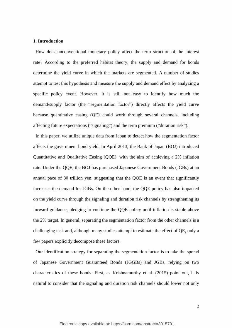
1. Introduction
How does unconventional monetary policy affect the term structure of the interest
rate? According to the preferred habitat theory, the supply and demand for bonds
determine the yield curve in which the markets are segmented. A number of studies
attempt to test this hypothesis and measure the supply and demand effect by analyzing a
specific policy event. However, it is still not easy to identify how much the
demand/supply factor (the “segmentation factor”) directly affects the yield curve
because quantitative easing (QE) could work through several channels, including
affecting future expectations (“signaling”) and the term premium (“duration risk”).
In this paper, we utilize unique data from Japan to detect how the segmentation factor
affects the government bond yield. In April 2013, the Bank of Japan (BOJ) introduced
Quantitative and Qualitative Easing (QQE), with the aim of achieving a 2% inflation
rate. Under the QQE, the BOJ has purchased Japanese Government Bonds (JGBs) at an
annual pace of 80 trillion yen, suggesting that the QQE is an event that significantly
increases the demand for JGBs. On the other hand, the QQE policy has also impacted
on the yield curve through the signaling and duration risk channels by strengthening its
forward guidance, pledging to continue the QQE policy until inflation is stable above
the 2% target. In general, separating the segmentation factor from the other channels is a
challenging task and, although many studies attempt to estimate the effect of QE, only a
few papers explicitly decompose these factors.
Our identification strategy for separating the segmentation factor is to take the spread
of Japanese Government Guaranteed Bonds (JGGBs) and JGBs, relying on two
characteristics of these bonds. First, as Krishnamurthy et al. (2015) point out, it is
natural to consider that the signaling and duration risk channels should lower not only

3
JGB yields but also JGGB yields in the same way, such that taking the spread of JGBs
and JGGBs enables us to cancel out these two components. Second, the important
institutional feature of QQE is that the BOJ does not purchase JGGBs. This means that
a demand shock caused by the BOJ only affects JGBs, not JGGBs. We note that JGGBs
are an identical asset to JGBs except in relation to liquidity. Exploiting this clear
characteristic as a laboratory, we decompose the spread into the segmentation and
liquidity factors.
Our result shows that the arbitrage between JGBs and JGGBs should be sufficient
during times when the JGB yields are positive, suggesting that the segmentation factor
has a relatively small effect on determination of the yield curve. However, the
importance of the segmentation factor is drastically amplified when the JGB yields
become negative. Intuitively, although the purchases by the BOJ push the JGB yields
deep into negative territory, there are no investors for JGGBs if the yields hit the zero
lower bound (ZLB). Figure 1 shows the time series for the spread of JGGBs and JGBs,
indicating that only the JGB yields have become negative, whereas the JGGB yields hit
the ZLB. This suggests that the markets clearly exhibit segmentation among JGBs and
JGGBs. This result is consistent with the theoretical implications proposed by Vayanos
and Vila (2009) and Greenwood and Vayanos (2014). In these papers, the arbitrageurs
absorb shocks to the demand and supply of a specific maturity’s bonds and, if the
arbitrageurs are confronted with a large limitation to arbitrage, the term structure of the
bond shows extreme segmentation.
The mechanism of the market segmentation between JGBs and JGGBs under ZLB is
quite simple. The JGB yield can move into negative territory because the BOJ

4
purchases JGBs with a negative yield.1 From the investors’ points of view, even if they
hold JGBs with negative yields, they can earn the zero yield (or even a positive return)
as long as the BOJ purchases JGBs with a negative yield. On the other hand, JGGBs
have not been purchased by the BOJ and, therefore, investors have no incentive to buy
JGGBs that yield an interest rate of less than zero.
Our paper is related to several strands of literature that focus on the segmentation
factor using spreads. Krishnamurthy and Vissing-Jorgensen (2011) study the Federal
Reserve quantitative easing policies during 2008–11, using the spread between the very
highest quality corporate bonds and comparable maturity government debt.
Krishnamurthy and Vissing-Jorgensen (2012) find that the higher is the supply of
government debt, the larger is the spread of the very highest quality corporate bonds.
Badoer and James (2016) present results that are consistent with Krishnamurthy and
Vissing-Jorgensen (2011, 2012). Krishnamurthy et al. (2015) focus on the spread
between the OIS swap rate and government bond yields to evaluate the European
Central Bank’s policy.
Our paper contributes to the existing literature in the following ways. First, this paper
is the first to describe how the ZLB affects the term structure in the context of the
preferred habitat theory. Numerous studies, including Dai et al. (2007), Koeda (2013),
and Christensen (2015), use regime switch models to examine the dynamics of bond
yields, including ZLB. In contrast to these studies, in our paper, identification is
achieved by using the institutional information of QQE, under which the BOJ only
purchases JGBs (not JGGBs), and we provide an interpretation of the regime shift in the
context of the preferred habitat theory.
1 The BOJ purchased JGBs with negative yields for the first time on September 9, 2014. This
preceded the implementation of the QQE with a Negative Interest Rate policy.

5
Second, compared with the previous studies, we utilize an asset that is more ideal for
analysis, the government guaranteed bond. For example, Krishnamurthy and
Vissing-Jorgensen (2011, 2012) and Krishnamurthy et al. (2015) are based on a
significant nondefault component, although high rated bonds and the OIS swap rate
could contain a slight default risk or a counterparty risk. To overcome this problem, we
use the JGGB, which has the same credit risk as the JGB and nonderivative assets. In
addition, our paper extends the existing literature by for the first time explicitly dealing
with the liquidity factor, which is nonnegligible for the asset pricing.
Third, we construct a liquidity measure using the spread of JGGBs and JGBs,
controlling for the segmentation factor. The liquidity measure is available publically
through our website (https://sites.google.com/site/hattori0819/data). Although there are
many studies that construct the liquidity measure by interpreting the spread of
government guaranteed bonds and government bonds, this is the first paper to explicitly
control the segmentation factor in this literature.
The remainder of the paper is organized as follows. Section 2 describes the features of
QQE and JGGBs. Section 3 contains the model and estimation strategy and Section 4
describes the data. Section 5 presents the results and the robustness check and Section 6
concludes.
2. Description of QQE and JGGBs
2.1 Government guaranteed bonds as a liquidity premium under positive JGB yields
Incorporated administrative agencies run businesses for public purposes in Japan in
their role as government agencies. The central government guarantees their debt up to a
maximum amount provided in the budget. The incorporated administrative agencies
issue bonds and the central government explicitly and fully guarantees these bonds. In
6
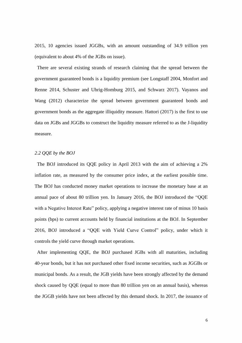
2015, 10 agencies issued JGGBs, with an amount outstanding of 34.9 trillion yen
(equivalent to about 4% of the JGBs on issue).
There are several existing strands of research claiming that the spread between the
government guaranteed bonds is a liquidity premium (see Longstaff 2004, Monfort and
Renne 2014, Schuster and Uhrig-Homburg 2015, and Schwarz 2017). Vayanos and
Wang (2012) characterize the spread between government guaranteed bonds and
government bonds as the aggregate illiquidity measure. Hattori (2017) is the first to use
data on JGBs and JGGBs to construct the liquidity measure referred to as the J-liquidity
measure.
2.2 QQE by the BOJ
The BOJ introduced its QQE policy in April 2013 with the aim of achieving a 2%
inflation rate, as measured by the consumer price index, at the earliest possible time.
The BOJ has conducted money market operations to increase the monetary base at an
annual pace of about 80 trillion yen. In January 2016, the BOJ introduced the “QQE
with a Negative Interest Rate” policy, applying a negative interest rate of minus 10 basis
points (bps) to current accounts held by financial institutions at the BOJ. In September
2016, BOJ introduced a “QQE with Yield Curve Control” policy, under which it
controls the yield curve through market operations.
After implementing QQE, the BOJ purchased JGBs with all maturities, including
40-year bonds, but it has not purchased other fixed income securities, such as JGGBs or
municipal bonds. As a result, the JGB yields have been strongly affected by the demand
shock caused by QQE (equal to more than 80 trillion yen on an annual basis), whereas
the JGGB yields have not been affected by this demand shock. In 2017, the issuance of
7
JGBs was about 103 trillion yen (on an annual basis)2, with 935 trillion yen of
outstanding JGBs, indicating that the BOJ purchases 78% of JGBs issued and 9% of
JGBs outstanding.
The BOJ has strengthened the forward guidance of the QQE in two ways.3 First, it has
released a statement of its intention to achieve the 2% price target as early as possible,
with a time horizon of about two years. Second, the BOJ has stated its intention to
continue with QQE as long as it is necessary to maintain the 2% target in a stable
manner. This forward guidance policy should affect the yield curve through the
channels of the expectation hypothesis and the term premium.
3. Model and Estimation Strategy
3.1 Determinants of the yields of JGBs and JGGBs
Following Krishnamurthy et al. (2015), we decompose the JGB yield into several
components:
r𝑡𝐽𝐺𝐵(𝑇) =
1
𝑇∫ 𝐸[𝑖𝑡]𝑑𝑡 + 𝑇𝑒𝑟𝑚𝑃𝑟𝑒𝑚𝑖𝑢𝑚𝑡(𝑇)𝑇
0+𝐶𝑟𝑒𝑑𝑖𝑡𝑅𝑖𝑠𝑘𝑡
𝐽𝐺𝐵(𝑇) + 𝑆𝑒𝑔𝑡𝐽𝐺𝐵(𝑇). (1)
The first component is the expectations hypothesis component of the yield (the
“signaling channel”) and the second component is a term premium (the “duration
channel”). The third component reflects the premium for sovereign risk and the last
component is the segmentation factor. The segmentation factor arises if the investors
confront some limitation to arbitrage and this factor becomes negative when this factor
2 This sum excludes redemption of the National Debt from the total issuance of the interest-bearing
bond (117.4 trillion JPY). 3 See http://www.bis.org/review/r140304c.pdf for details.

8
reduces the yield.
We model the yield of JGGBs as follows:
r𝑡𝐽𝐺𝐺𝐵(𝑇) =
1
𝑇∫ 𝐸[𝑖𝑡]𝑑𝑡 + 𝑇𝑒𝑟𝑚𝑃𝑟𝑒𝑚𝑖𝑢𝑚𝑡(𝑇) + 𝐶𝑟𝑒𝑑𝑖𝑡𝑅𝑖𝑠𝑘𝑡
𝐽𝐺𝐵(𝑇)𝑇
0
+
𝐿𝑖𝑞𝑢𝑖𝑑𝑖𝑡𝑦𝑡(𝑇)+𝑆𝑒𝑔𝑡𝐽𝐺𝐺𝐵(𝑇). (2)
The first, second, and third components of eq. (2) are identical to those of eq. (1). The
credit risk of JGBs and JGGBs is identical because the Japanese government explicitly
guarantees JGGBs. The fourth component is the liquidity factor, which is in sharp
contrast to Krishnamurthy et al. (2015). Previous studies (see Vayanos and Wang 2012
and Schwarz 2017) treat the spread between the government guaranteed bond and the
government bond as the aggregate illiquidity measure, concluding that this modeling is
a natural extension of Krishnamurthy et al. (2015). The final component is a
segmentation factor of JGGBs. To identify the segmentation factor, we differentiate eqs.
(1) and (2), as follows:
𝑆𝑝𝑟𝑒𝑎𝑑𝑡(𝑇) = 𝐿𝑖𝑞𝑢𝑖𝑑𝑖𝑡𝑦𝑡(𝑇) + 𝑆𝑒𝑔𝑡(𝑇). (3)
This equation shows the spread of JGGBs and JGBs, decomposed into the liquidity
and segmentation factors ( 𝑆𝑒𝑔𝑡(T) ≔ 𝑆𝑒𝑔𝑡𝐽𝐺𝐺𝐵(𝑇) − 𝑆𝑒𝑔𝑡
𝐽𝐺𝐵(𝑇) ). 𝑆𝑝𝑟𝑒𝑎𝑑𝑡(𝑇)
increases (decreases) when 𝑆𝑒𝑔𝑡𝐽𝐺𝐵(𝑇) decreases (increases) the JGB yields. As we
have already pointed out, QQE policy has only affected JGBs (not JGGBs) and the
demand for JGBs is dominated by the BOJ under its QQE policy. Thus, 𝑆𝑒𝑔𝑡(T)
should reflect the demand for JGBs from the BOJ after 2013/4. 𝑆𝑝𝑟𝑒𝑎𝑑𝑡(𝑇) should

9
increase when the QQE affects the demand for JGBs as long as the liquidity factor is
stable.
3.2 Kalman filter and identification
Now, we represent eq. (3) as the state-space representation and use Kalman filtering to
decompose the spread into the liquidity and segmentation factors. The state-space model
is best suited to our analysis for two reasons. First, it enables the measurement problem
to be overcome explicitly. As Bank of Japan (2017) and Hattori (2017) show, the
movement of the bond liquidity could depend on the definition of the liquidity measure,
suggesting that the liquidity measure could contain measurement errors. Second, this
approach is supported by the existing literature and is commonly used for decomposing
the yield spread; see, for example, Feldhütter and Lando (2008) and Krishnamurthy et al.
(2015).
To use the state-space representation, we assume that the liquidity and segment factors,
which are the state variables, follow a first-order vector autoregression:
[𝑥1,𝑡𝑥2,𝑡
] = [𝛼1𝛼2] + [
𝛽1 00 𝛽2
] [𝑥1,𝑡−1𝑥2,𝑡−1
] + [𝑢1𝑡𝑢2𝑡
], (4)
where 𝑢𝑡 is a vector of mutually uncorrelated standard normal disturbances.
The measurement equation is:
[𝑦1,𝑡𝑦2,𝑡
] = 𝐻 [𝑥1,𝑡𝑥2,𝑡
] + [𝑤1𝑡
𝑤2𝑡] = [
1 10 1
] [𝑥1,𝑡𝑥2,𝑡
] + [𝑤1𝑡
𝑤2𝑡], (5)
where 𝑤𝑡 is a vector of mutually uncorrelated standard normal disturbances. As in

10
Krishnamurthy et al. (2015), identification should be made by the choice of H. In Table
1, we present our identification. As eq. (3) indicates, the spread of JGGBs and JGBs
should be affected simultaneously by the liquidity and segmentation factors. On the
other hand, the liquidity measure should be affected only by the liquidity factor.
We use a Kalman filter and smoother to extract the unobserved factor 𝑥𝑡 to use the
observed 𝑦𝑡.
4. Data
4.1 Measurement of liquidity
We use the yield curve fitting noise as the measure of the liquidity factor in eq. (5).
The yield curve fitting error is the liquidity measure proposed by Hu et al. (2013).
Vayanos and Wang (2012) summarize this measure and the government guaranteed
bond spreads as the aggregate liquidity measure, so it is natural to use the yield curve
fitting error as the measure of the liquidity factor in eq. (5).
Following Hu et al. (2013), we construct the noise measure by fitting daily data for
JGBs into a smooth yield curve, using the approach in Svensson (1994), and then
compute the mean squared errors as the illiquidity premium. The yield curve fitting
noise is calculated on a daily basis. For a robustness check, we also use the bid–ask
spread of the JGB yields.
4.2 Data description
We estimate the zero-coupon yield of JGBs and JGGBs using Reference Statistical
Prices [Yields] for OTC Bond Transactions, compiled by the Japan Securities Dealers
Association (JSDA). The JSDA collects bond prices and coupons on a daily basis from
18 main securities firms and provides the data on its website. We employ a spline-based

11
approach to estimate the zero-coupon yield. Following Steeley (1991) and Kikuchi and
Shintani (2012), we interpolate the discount factors based on the B-spline method.
We use the JSDA data to compute the yield curve fitting noise. We remove from the
data the T-bills and coupon-bearing bonds with remaining maturities of more than 10
years. In addition, we use the bid–ask spread of JGBs from Bloomberg as our
alternative measure of the liquidity premium. The bid–ask spread is constructed using
10-year on-the-run JGBs.
Table 2 shows the fundamental statistics of the yield curve fitting noise and bid–ask
spreads. The means (standard deviations) of the yield curve fitting noise and bid–ask
spreads are 1.19 bps (0.33 bps) and 1.19 bps (0.37 bps), respectively, which indicates
that the liquidity premiums measured using these definitions are very similar.
5. Estimation Results
5.1 Decomposition of the spread of JGBs and JGGBs
Figure 2 depicts the two-year, five-year, and 10-year segmentation and liquidity factors,
which are decomposed by the Kalman filter. Table 3 shows the estimation results. As
noted in Section 3.2, the measurement of the liquidity factor for Kalman filtering is the
yield curve fitting noise proposed by Hu et al. (2013); this measurement method will be
replaced with the alternative method for a robustness check in the next section.
Figure 2 highlights three facts. First, the segmentation factor was low and stable during
the time when the JGB yield remained positive. This implies that the signaling and
duration channels were the main causes of the large reduction in interest rates after the
introduction of the QQE and that the arbitrage between JGGBs and JGBs was sufficient
during this period.
Second, the segmentation factor increased during the time when the JGB yield

12
became negative, indicating that the market for JGBs and JGGBs was sharply
segmented. We interpret that the segmentation factor of JGBs (𝑆𝑒𝑔𝑡𝐽𝐺𝐵(𝑇)) was largely
responsible for the increase in the segmentation factor (𝑆𝑒𝑔𝑡(T)). As noted in Section 3,
the segmentation factor of JGBs (𝑆𝑒𝑔𝑡𝐽𝐺𝐵(𝑇)) should have a negative value when the
BOJ’s demand as a result of the QQE pushes the JGB yield into negative territory. In
addition, the segmentation factor of JGGBs (𝑆𝑒𝑔𝑡𝐽𝐺𝐺𝐵(𝑇)) should remain unchanged
during the period when JGGBs hit the ZLB because investors have no incentive to hold
negative-yield JGGBs and the demand for JGGBs could not change in this
circumstance.
Third, the two-year segmentation factor was larger than the 10-year segmentation
factor during the period when the market segmented because the short-term JGB yields
fell much more deeply into negative territory. In contrast, particularly after the end of
2016, the 10-year JGB yields became positive, driving a decrease in the segmentation
factor.
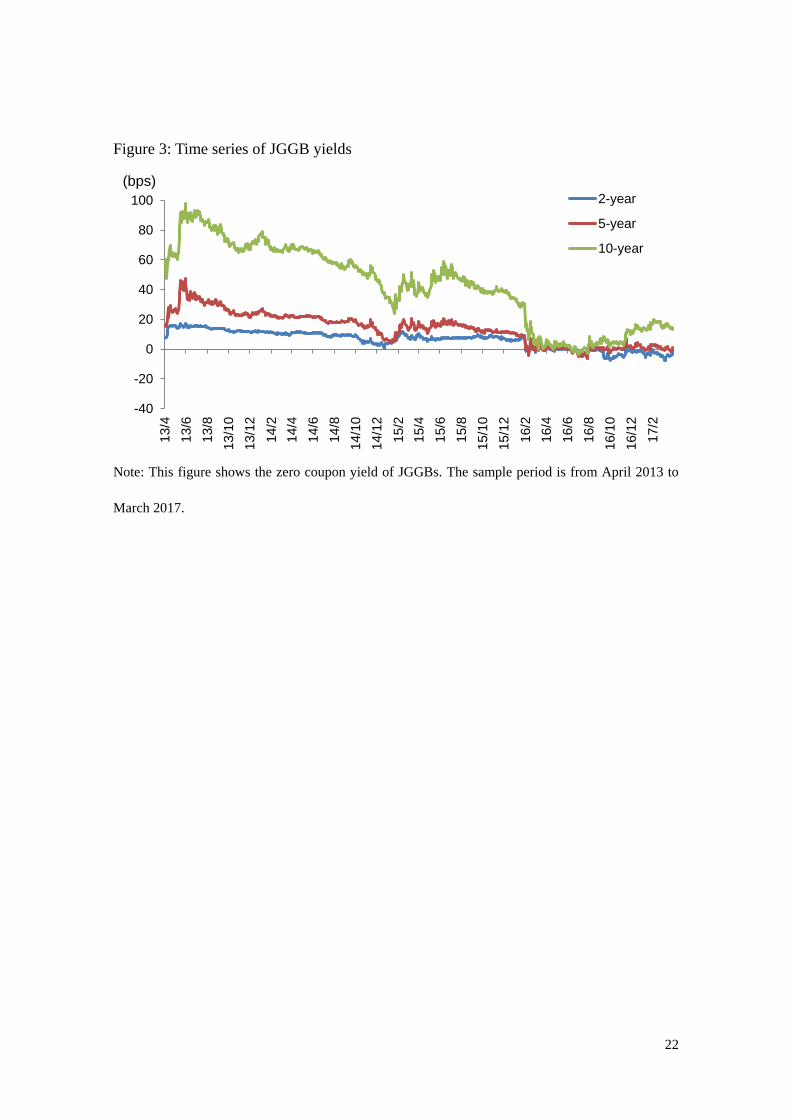
As noted in the Introduction, the mechanism of the market segmentation between
JGBs and JGGBs under ZLB is as follows. The JGB yields are able to move into
negative territory because the BOJ purchases JGBs with negative yields. On the other
hand, JGGBs have not been purchased by the BOJ, so that there is no incentive for
investors to buy JGGBs that yield an interest rate of less than zero. Figure 3 shows the
time series of JGGB yields, clearly indicating that the JGGB yields hit the ZLB and that
the segmentation factor of JGGBs (𝑆𝑒𝑔𝑡𝐽𝐺𝐺𝐵(𝑇)) could not be negative, in contrast to
the segmentation factor of JGBs (𝑆𝑒𝑔𝑡𝐽𝐺𝐵(𝑇)).
The Kalman filter enables us to separate the segmentation and liquidity factors from
the spread of JGGBs and JGBs and we have uploaded this liquidity measure on our
13
website (https://sites.google.com/site/hattori0819/data) for future research. Hattori
(2017) interprets the spread of JGGBs and JGBs as a liquidity premium, referring to it
as the “J-liquidity measure”. Thus, we refer to our new estimate of the liquidity measure
as the “modified J-liquidity measure”.
5.2 Robustness check
In this section, we conduct the robustness check. We examine an alternative measure
of the liquidity factor and find our results to be robust. As noted in Section 3.2, we use
the bid–ask spread of 10-year on-the-run JGBs as the measure of the liquidity factor.
Figure 4 shows the decomposition of the JGGB spread based on this alternative
measure and confirms the same trend found as discussed in Section 4.1. The
segmentation factor was low and stable during the time when the JGB yields remained
positive, but increased when the JGB yields became negative. The short-term
segmentation factor was larger than the long-term segmentation factor.
The difficulty is that there is limited availability of data on the liquidity premium on a
daily basis. However, we consider that our results are robust because the other liquidity
measure, made on a monthly basis, is stable during the time when JGB yields became
negative (the spread of JGGBs and JGBs increased drastically). Figure 5 shows the
Amihud (2002) measure and turnover, which are the liquidity measures made on a
monthly basis (see the definition in the Appendix) as well as the yield curve fitting noise
and the bid–ask spread, indicating that these measures are relatively stable when the
JGB yields become negative. These facts also confirm that the liquidity factor was
stable during the time when the JGB yields became negative, suggesting that the
segmentation factor strengthens when the JGB yields become negative.

14
6. Conclusion
This paper attempts to show that the segmentation factor has strengthened when
arbitrageurs face limits to arbitrage. To accomplish this goal, we focus on JGGBs,
which are an identical asset to JGBs except for their liquidity, and we take the spread of
these yields to control for the signaling and duration channels. Significantly, under the
QQE, the BOJ exclusively purchases JGBs, so we can utilize the different treatment of
JGBs and JGGBs under the QQE.
Our results indicate that the spread increased sharply when the JGGB yields hit the
ZLB, although the spread is relatively stable as long as the JGB yields are positive. The
negative yields of JGGBs discourage arbitrageurs from holding JGGBs, but they still
purchase JGBs because the BOJ purchases JGBs with negative yields. This situation
creates a structural break in the arbitrage activities between JGGB and JGB markets,
making the market segmented. Our results contribute to the existing literature on the
preferred habit theory, proposed by Vayanos and Vila (2009) and Greenwood and
Vayanos (2014), and to the empirical research on segmentation factors (Krishnamurthy
and Vissing-Jorgensen 2011, 2012, Krishnamurthy et al. 2015).
In addition, we contribute to the literature with the liquidity measure that we have
developed. Many studies focus on government guaranteed bonds to construct liquidity
premiums, but the existing literature does not explicitly examine segmentation factors.
We have provided these data on our website to assist future academic research.

15
REFERENCES
Amihud, Y., 2002. Illiquidity and stock returns: cross-section and time series effects.
Journal of Financial Markets 5, 31–56.
Badoer. D., James, C., 2016. The determinants of long-term corporate debt issuances.
The Journal of Finance 71 (1), 457–492.
Bank of Japan., 2017. Liquidity Indicators in the JGB Markets.
Christensen, J., 2015. A Regime-Switching Model of the Yield Curve at the Zero
Bound. Federal Reserve Bank of San Francisco Working Paper 2013-34.
Dai, Q., Singleton, K., Yang, W., 2007. Regime shifts in a dynamic term structure
model of U.S. treasury bond yields. Review of Financial Studies, 20 (5), 1669–1706.
Greenwood, R., Vayanos, D., 2014. Bond supply and excess bond returns. Review of
Financial Studies 27 (3), 663–713.
Feldhütter, P., Lando, D., 2008. Decomposing swap spreads. Journal of Financial
Economics 88, 375–405.
Hattori, T., 2017. J-liquidity Measure: The Term Structure of the Liquidity Premium
and the Decomposition of the Municipal Bond Spread. PRI Discussion Paper Series (No.
17A-03).
Hu, X., Pan, J., Wang, J., 2013. Noise as information for illiquidity. The Journal of
Finance 68 (6), 2341–2382.
Kikuchi, K., Shintani, K., 2012. Comparative analysis of zero coupon yield curve
estimation methods using JGB price data. Monetary and Economic Studies 30.
Koeda, J., 2013. Endogenous monetary policy shifts and the term structure: evidence
from Japanese Government Bond yields. Journal of the Japanese and International
Economies, 29, 170–188.
Krishnamurthy, A., Nagel, S., Vissing-Jørgensen, A., 2015. ECB policies involving
government bond purchases: impact and channels. Unpublished working paper,
Stanford University, University of Michigan and University of California Berkeley.
Krishnamurthy, A., Vissing-Jorgensen, A., 2011. The effects of quantitative easing on
interest rates: channels and implications for policy. Brookings Papers on Economic
Activity Fall, 215–265.
Krishnamurthy, A., Vissing-Jorgensen., A., 2012. The aggregate demand for Treasury
debt. Journal of Political Economy 120 (2), 233–267.

16
Longstaff, F.A., 2004. The flight-to-liquidity premium in U.S. Treasury bond prices.
Journal of Business 77, 511–526.
Monfort, A., Renne, J.-P., 2014. Decomposing euro-area sovereign spreads: credit and
liquidity risks. Review of Finance 18, 2103–2151.
Schwarz, K., 2017. Mind the Gap: Disentangling Credit and Liquidity in Risk Spreads.
Working Paper.
Schuster, P., Uhrig-Homburg, M., 2015. Limits to arbitrage and the term structure of
bond illiquidity premiums. Journal of Banking and Finance 57, 143–159.
Steeley, J., 1991. Estimating the gilt-edged term structure: basis splines and confidence
intervals. Journal of Business, Finance and Accounting, 18 (4), 513–29.
Svensson, L.E.O., 1994. Estimating and Interpreting Forward Rates: Sweden 1992–
1994. Unpublished working paper 4871. National Bureau of Economic Research,
Cambridge, MA.
Vayanos, D., Vila, J.-L., 2009. A Preferred-habitat Model of the Term Structure of
Interest Rates. Unpublished working paper. London School of Economics, London, UK.
Vayanos, D., Wang, J., 2012. Market Liquidity—Theory and Empirical Evidence.
NBER Working Paper, 18251.
17
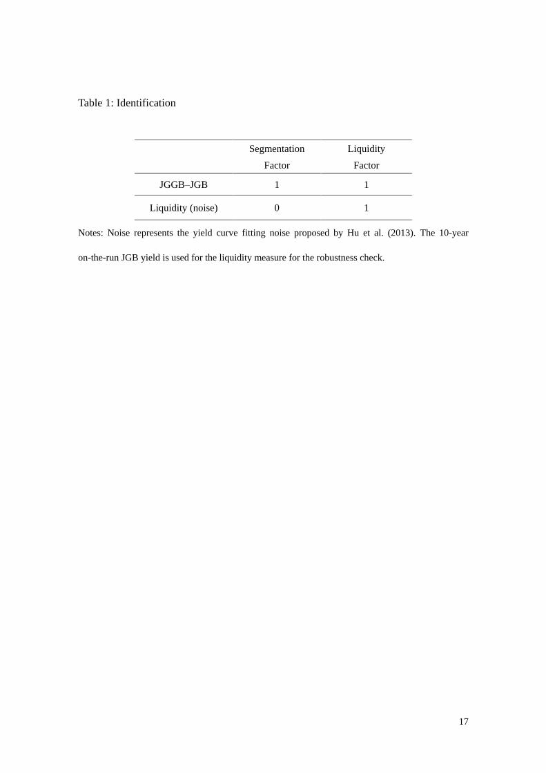
Table 1: Identification
Segmentation
Factor
Liquidity
Factor
JGGB–JGB 1 1
Liquidity (noise) 0 1
Notes: Noise represents the yield curve fitting noise proposed by Hu et al. (2013). The 10-year
on-the-run JGB yield is used for the liquidity measure for the robustness check.

18
Table 2: Summary Statistics
N Mean Median Max Min SD Skewness Kurtosis JB
Yield curve
fitting noise 979 1.19 1.18 2.61 0.56 0.33 0.71 4.13 135
Bid–ask spread 979 1.19 1.00 3.00 0.50 0.37 2.81 12.31 4,831
Notes: This table shows the summary statistics for the yield curve fitting noise and the bid–ask
spread of 10-year on-the-run JGB yields. JB stands for Jarque–Bera test statistic. The sample period
is from April 2013 to March 2017. The data frequency is daily.

19
Table 3: Estimation Results
Parameters 2-year 5-year 10-year
1 0.0071 0.0071 0.0138
(0.016) (0.016) (0.019)
2 0.0582 0.0579 0.0648
(0.013) (0.013) (0.014)
1 0.9992 0.9992 0.9952
(0.001) (0.001) (0.001)
2 0.9717 0.9718 0.9683
(0.006) (0.006) (0.007)
No. of Obs. 1472 1472 1472
Notes: This table presents the parameter estimates resulting from the Kalman filters. The t-statistics
are presented in parentheses.

20
Figure 1: The spread of JGGBs and JGBs (5-year)
Notes: This figure shows the time series of yield of 5-year JGBs and 5-year JGGBs. We interpret the
spread of JGGBs and JGBs as the sum of the liquidity and segmentation factors. The sample period
is from April 2013 to March 2017. The data frequency is daily.
0
5
10
15
20
25
30
35
-50-40-30-20-10
0102030405060
13/4
13/6
13/8
13/1
0
13/1
2
14/2
14/4
14/6
14/8
14/1
0
14/1
2
15/2
15/4
15/6
15/8
15/1
0
15/1
2
16/2
16/4
16/6
16/8
16/1
0
16/1
2
17/2
JGB:5-year JGGB:5-year Difference:Liquidity+Segmentation(right)
(bps)

21
Figure 2: Estimation results (yield curve fitting noise)
2-year
5-year
10-year
Note: This figure shows the decomposition of the spread of JGGBs and JGBs into the segmentation
and liquidity factors based on the Kalman filter. The measurement of the liquidity factor uses the
yield curve fitting noise proposed by Hu et al. (2013). The highlighted period indicates when the
JGB yields were negative. The sample period is from April 2013 to March 2017.
-10
0
10
20
30
40
13
/4
13
/6
13
/8
13
/10
13
/12
14
/2
14
/4
14
/6
14
/8
14
/10
14
/12
15
/2
15
/4
15
/6
15
/8
15
/10
15
/12
16
/2
16
/4
16
/6
16
/8
16
/10
16
/12
17
/2
negative yield zone
segmentation factor
liquidity factor
(bps)
-10
0
10
20
30
40
13/4
13/6
13/8
13/1
0
13/1
2
14/2
14/4
14/6
14/8
14/1
0
14/1
2
15/2
15/4
15/6
15/8
15/1
0
15/1
2
16/2
16/4
16/6
16/8
16/1
0
16/1
2
17/2
negative yield zone
segmentation factor
liquidity factor
(bps)
-505
101520253035
13/4
13/6
13/8
13/1
0
13/1
2
14/2
14/4
14/6
14/8
14/1
0
14/1
2
15/2
15/4
15/6
15/8
15/1
0
15/1
2
16/2
16/4
16/6
16/8
16/1
0
16/1
2
17/2
negative yield zone
segmentation factor
liquidity factor
(bps)
22
Figure 3: Time series of JGGB yields
Note: This figure shows the zero coupon yield of JGGBs. The sample period is from April 2013 to
March 2017.
-40
-20
0
20
40
60
80
100
13/4
13/6
13/8
13/1
0
13/1
2
14/2
14/4
14/6
14/8
14/1
0
14/1
2
15/2
15/4
15/6
15/8
15/1
0
15/1
2
16/2
16/4
16/6
16/8
16/1
0
16/1
2
17/2
2-year
5-year
10-year
(bps)

23
Figure 4: Estimation results (bid–ask spread)
2-year
5-year
10-year
Note: This figure shows the decomposition of the spread of JGGBs and JGBs into the segmentation
and liquidity factors, based on the Kalman filter. The measurement of the liquidity factor is based on
the bid–ask spread of 10-year on-the-run JGBs. The highlighted period indicates when the JGB
yields became negative.
0
10
20
30
40
13/4
13/6
13/8
13/1
0
13/1
2
14/2
14/4
14/6
14/8
14/1
0
14/1
2
15/2
15/4
15/6
15/8
15/1
0
15/1
2
16/2
16/4
16/6
16/8
16/1
0
16/1
2
17/2
negative yield zone
segmentation factor
liquidity factor
0
10
20
30
40
13/4
13/6
13/8
13/1
0
13/1
2
14/2
14/4
14/6
14/8
14/1
0
14/1
2
15/2
15/4
15/6
15/8
15/1
0
15/1
2
16/2
16/4
16/6
16/8
16/1
0
16/1
2
17/2
negative yield zone
segmentation factor
liquidity factor
-5
0
5
10
15
20
25
30
35
13/4
13/6
13/8
13/1
0
13/1
2
14/2
14/4
14/6
14/8
14/1
0
14/1
2
15/2
15/4
15/6
15/8
15/1
0
15/1
2
16/2
16/4
16/6
16/8
16/1
0
16/1
2
17/2
negative yield zone
segmentation factor
liquidity factor

24

25
Figure 5: Other liquidity measures
Note: This figure shows the liquidity measure on a monthly basis (noise, turnover, Amihud, bid–ask
spread). The noise and turnover use the monthly average of the daily base data. The definitions of
Amihud and turnover are provided in the Appendix. The sample period is from April 2013 to March
2017.
-2
-1
0
1
2
3
4
13/4
13/6
13/8
13/1
0
13/1
2
14/2
14/4
14/6
14/8
14/1
0
14/1
2
15/2
15/4
15/6
15/8
15/1
0
15/1
2
16/2
16/4
16/6
16/8
16/1
0
16/1
2
17/2
noise turnover Amihud bidaskspread

26
Appendix
1. Amihud measure
Amihud (2002) constructs an illiquidity measure, defined as the following ratio:
𝐴𝑚𝑖ℎ𝑢𝑑 = 𝑎𝑣𝑒𝑟𝑎𝑔𝑒 (|𝑟𝑡|
𝑉𝑜𝑙𝑢𝑚𝑒𝑡),
where 𝑟𝑡 is the return and 𝑉𝑜𝑙𝑢𝑚𝑒𝑡 is the trading volume on day 𝑡. This captures the
price impact, reflecting the price response associated with trading volume. We calculate
this measure using daily data on JGB futures from Bloomberg and compute the monthly
average.
2. Turnover (negative)
The annualized turnover is the annualized trading volume divided by the amount
outstanding. To convert this to a measure of illiquidity, we take the negative of turnover.