Market Quality and Contagion in

Fragmented Markets

Rohit Rahi

Jean-Pierre Zigrand

SRC Discussion Paper No 2

September 2013

ISSN xxx-xxxx

Abstract Financial market liquidity has become increasingly fragmented across multiple trading platforms. We propose an intuitive welfare-based market quality metric that can properly aggregate local market conditions across both securities and trading venues. Our analysis rests on a general equilibrium model with segmented markets. Arbitrageurs reap profits by effectively providing intermediation services (i.e. “liquidity"). Our market quality measure is equal to the additional consumption enjoyed by investors as a result of this intermediation, and can be represented by means of a number of observable proxies. The model is especially well-suited to study the contagion-like effects of liquidity shocks. JEL classification: G10, G20, D52, D53. Keywords: Fragmented markets, intermediation, arbitrage, liquidity, contagion. This paper is published as part of the Systemic Risk Centre’s Discussion Paper Series. The support of the Economic and Social Research Council (ESRC) in funding the SRC is gratefully acknowledged [grant number ES/K002309/1]. Acknowledgements This paper was circulated earlier under the title “A Theory of Strategic Intermediation and Endogenous Liquidity”. The authors thank the late Sudipto Bhattacharya, Douglas Gale, Joel Peress, Tano Santos, José Scheinkman as well as participants at workshops and seminars at several universities for helpful discussions. Rohit Rahi is Reader in Finance at the Department of Finance and Financial Markets Group, and Research Associate of Systemic Risk Centre, London School of Economics and Political Science. Jean-Pierre Zigrand is Reader in Finance at the Department of Finance and Financial Markets Group, and Co-Director of Systemic Risk Centre, London School of Economics and Political Science. Published by Systemic Risk Centre The London School of Economics and Political Science Houghton Street London WC2A 2AE All rights reserved. No part of this publication may be reproduced, stored in a retrieval system or transmitted in any form or by any means without the prior permission in writing of the publisher nor be issued to the public or circulated in any form other than that in which it is published. Requests for permission to reproduce any article or part of the Working Paper should be sent to the editor at the above address. © R Rahi, J-P Zigrand, submitted 2013

1 Introduction

One of the most disruptive recent changes in the financial industry has been thewidespread proliferation of trading venues following the Regulation National MarketSystem (Reg NMS) in the US and the Markets in Financial Instruments Directive(MiFID) in Europe. The same stocks are traded not only on several exchanges butalso on alternative trading systems such as Multilateral Trading Facilities (MTFs),Electronic Communication Networks (ECNs) and various Dark Pools.1 The regu-lations, which were designed to enhance competition between trading venues, havein turn spawned a new breed of intermediary in the form of high-frequency traders(HFTs) or latency arbitrageurs2 who trade simultaneously across multiple tradingvenues in order to exploit, and thus reduce or eliminate, price discrepancies. A verylarge percentage of trading volume has been attributed to such traders.3 There isgrowing concern that competition in security markets in the US and Europe has ledto trading liquidity becoming fragmented across too many venues. At the same time,the HFTs, who provide liquidity and help to align prices across venues, have beenviewed with suspicion by the press, the traditional real-money investors and even bythe regulators who to some extent created the need for this intermediation.

The Flash Crash of May 6th 2010, in which the Dow Jones index fell nearly10% only to recover a few minutes later, has accelerated that discussion and hasbrought the topic of modern market making to the forefront. Attention has focusedon the interconnectedness of trading venues and the implications for liquidity andwelfare. For instance, a report by the CFTC and SEC (CFTC and SEC (2010))points out that during the Flash Crash, “hot-potato volumes” spiked up as HFTspassed securities around in a musical chair-like fashion within and across tradingvenues, and shocks were transmitted across markets for stocks, options and futuresin a complex fashion. When latency arbitrageurs withdrew from the markets andprices of identical securities diverged across trading venues, panic set in as market

1Examples at the time of writing are BATS (merged with Chi-X), Turquoise, Burgundy, ITGPosit, Equiduct, QuoteMTF, Liquidnet, UBS MTF, Sigma X MTF, Instinet Blockmatch, NomuraNX and Smartpool.

2Examples of HFTs include proprietary quantitative hedge funds and market makers at firmssuch as Citadel Group, D.E. Shaw Group, Renaissance Technologies, Getco, Optiver, Knight andTradebot, as well as trading desks in some of the major investment banks.

3Various sources estimate that the fraction of equity trades involving HFT algorithms is 60–70%in the US, 30% in the UK, 40% in Europe, and 30% in Japan (see, for instance, Beddington et al.(2013)). The TABB group estimates that annual aggregate profits from latency arbitrage currentlyexceed $21bn, Donefer (2008) provides a range of $15-25bn, and Strasbourg (2011) estimates thatHFT profits in the US were around $7.2bn in 2009. Other observers believe profits to be smaller.Even if these estimates are in the right ballpark, it is unfortunately not known what fraction ofthe profits are due to cross-trading-venue arbitrage as opposed to within-venue market making,although an indirect indication points to large profits: Kearns et al. (2010) have estimated that hadHFTs had perfect foresight, they could have reaped about $21bn of within-venue market makingprofits in US markets. Since HFTs do not have perfect foresight, actual within-venue profits arebound to be much smaller, and given the estimates of overall HFT profits, across-venue profits arelikely to be sizable.

2

participants no longer trusted the price discovery mechanism.4 This suggests thatconventional measures of intermediation and liquidity provision may not adequatelyreflect market conditions when trading and liquidity are fragmented.

And yet the bulk of academic research on financial markets still relies on a priceformation mechanism on a single centralized market, leaving regulators with no mod-eling tools to rigorously understand the impact of new policy initiatives designed toinfluence diverse trading platforms. In Europe, for instance, policy makers haveindicated that models that explicitly account for fragmented markets in a generalequilibrium setting are desperately needed to think through the MiFID 2 processthat is currently under review and to engage in economic impact and market qualityanalysis. They have also indicated that it is not sufficient to merely account forthe fact that the same stocks are traded across multiple trading venues, but thatthe model ought to be flexible enough to allow for stocks, derivatives on stocks,exchange-traded funds and related securities traded on distinct venues,5 while pro-viding guidance on how market quality is affected by fragmentation and the resultinglinkages created by latency arbitrageurs. This paper can be viewed as a first step inthat direction.

We propose a simple model that explicitly allows for multiple assets traded inmultiple markets or venues6 that are linked by profit-motivated arbitrageurs or in-termediaries. We specifically focus on cross-venue market making and abstract fromwithin-venue market making. We model intermediaries as imperfectly competitivewith entry into the intermediation business unrestricted but entailing a fixed cost(say in terms of human capital, software, or co-location of servers at the various mar-

4Consider for example the E-Mini index futures contract traded on CME Globex and the SPYexchange-traded fund traded on NYSE, both of which track the S&P500. During the Flash Crash,trading in the E-Mini was paused for 5 seconds while trading in SPY continued. Uncertaintiesabout pricing accuracy, exacerbated by the uncoordinated introduction of circuit breakers, ledmany arbitrageurs to cease operating their cross-market strategies. For four minutes, very profitablearbitrage mispricings occurred (for details see CFTC and SEC (2010) and Hunsader (2010)). For adetailed analysis of financial stability in computer-based trading environments, the reader is referredto Chapter 4 of Beddington et al. (2013).

5As an example, consider the SPY exchange-traded fund that we alluded to in footnote 4. SPYenters into a no-arbitrage relationship with the portfolio of equities underlying the S&P500 index.In addition, there are over 2000 options on SPY. Each such option needs to satisfy no-arbitragerelationships not only with SPY, but also with all sorts of combinations of other options on SPY.Furthermore, SPY options are traded on six options exchanges simultaneously, adding anotherlayer of law-of-one price relationships. Finally, options on SPY are closely related to options on theS&P500 itself as well as to options on the S&P500 futures contract.

6While the “venue” metaphor is a helpful one and fits some situations such as latency arbitragein which the same or similar securities are traded simultaneously on multiple trading venues, itis equally natural to think of the segmentation as being functional rather than geographical, e.g.in terms of investors restricted to certain asset classes (on-the-run versus off-the-run bonds, stockindex arbitrage, equities versus derivatives on those equities, investment grade versus junk bondsetc.). A trading venue can also be interpreted as an over-the-counter (OTC) market in which anintermediary trades with a clientele; the intermediary then tries to offload the exposure from thisOTC trade either with offsetting OTC counterparties or in the organized markets.

3

ket centers). Just as in the real world where latency arbitrageurs hit limit order bidsand asks by market orders (in the US by using intermarket sweep orders to bypassthe Order Protection Rule), the intermediaries in our model use market orders tohit the net excess demand schedules left by the marginal investors on each tradingvenue. In equilibrium, gains from trade are intermediated and local valuations andliquidities are aggregated across trading venues through an arbitrage network.

This framework allows us to address common questions about the fragmentedstructure of modern financial markets. If cross-venue arbitraging is competitive,are equilibrium allocations and prices identical to those that would obtain in aneconomy with a single centralized and perfectly competitive venue? What is theeffect of barriers to entry into the intermediation sector? What are the relationshipsbetween volumes, liquidity and welfare across trading venues? How is a liquidityshock affecting one venue transmitted through the entire network connected by suchintermediaries? Whatever the reputation of cross-venue arbitrageurs, they wouldseem to provide a valuable service and given the general equilibrium setting of ourmodel, we can answer welfare questions in a straightforward manner. Is the liquidityoffered by latency arbitrageurs welfare-improving, and if yes, how can it be measured?How can the overall welfare be disaggregated into the contributions of individualsecurities? If intermediaries can design and trade securities to extract maximumprofits, what is the effect on welfare?

We define market quality as the welfare gains achieved in equilibrium throughthe trading of securities via intermediaries. These gains are reflected in state pricesacross trading venues, before and after intermediation, and can be quantified asthe additional consumption enjoyed by investors as a result of the intermediation.Market quality can thus be viewed as intermediated liquidity that channels gainsfrom trade across multiple trading venues. Intermediaries provide liquidity in thevery direct sense of being the counterparties to trades made possible by their diversecustomer base that reaches across various clienteles or market centers.

Trading liquidity is often regarded as a salient feature of well-functioning secu-rity markets. Traditional liquidity metrics such as depth (the market impact of atrade), breadth (the size of bid-ask spreads), volume, transaction costs, as well astimeliness and ease of execution of trades can be viewed as symptoms or attributes ofan appropriate provision of liquidity that exploits gains from trade. Unfortunately,such measures are rarely welfare-based, not least because they view assets one byone and ignore interdependencies across assets and markets. A particular asset maynot be liquid in those metrics, but substitutes may be liquid enough to compensatefor it in a way that the underlying payoff is liquid. Looking at the liquidity of onesecurity or on one platform is therefore unlikely to reveal the whole story and a globalmetric is needed, such as the one proposed in this paper. We characterize some ofthe relationships between our metric and the conventional measures or attributes.While relying on the attributes themselves is no doubt useful for market practition-ers, thinking of them as sufficient proxies for market quality or overall welfare canbe misleading.

4

The main contributions of our paper are the following.First, and relative to conventional measures of liquidity, our metric is not only

welfare-based, but it also has the advantage that it can be aggregated and disag-gregated easily, across securities as well as trading venues. For instance, it is notobvious how one can infer the overall quality of a market from the spreads or vol-umes of individual securities. Usually this involves picking a few assets that aredeemed representative of the market as a whole. Furthermore, since identical assets,or more generally payoffs, may not exist on multiple trading venues, one would needto compare substitute assets. Both points raise a Pandora’s box of judgmental issueswhich can be avoided entirely by using a metric built on state prices instead.

Second, we derive useful proxies of our market quality metric that can in principlebe empirically estimated. One such proxy is equilibrium volume per unit of depth.Neither high volume nor depth are necessarily desirable attributes of a financialmarket, for if a market is deep and yet attracts little volume, it does not serve auseful role. Our measure of market quality can also be deduced directly from thecosts of entry into the intermediation sector, for such costs determine the degree ofcompetition between intermediaries and therefore the gains from trade realized.

Third, our model provides a coherent framework for understanding recent marketphenomena. For instance, much has been made of the design of unwise complexsecurities. We evaluate the impact on market quality of equilibrium asset innovationby intermediaries designed to extract the maximum surplus from investors (as isthe case for example with many categories of OTC derivatives). We find that suchinnovation enhances overall market quality, mainly because intermediaries find itoptimal in equilibrium to offer what investors desire – and are willing to pay for– most, though market quality in some sectors of the economy may be adverselyaffected.

Our model also provides a framework within which one can understand the logicof securitization. The boom in collateralized debt obligations (CDOs) was madepossible not only by the low interest rate environment, but also by the arbitrageprofits reaped by CDO structurers due to the difference between the price paid fordebt, and the monies raised by selling tranches of that debt tailored to the needsof individual clienteles. Our framework offers a rationale for the CDO mechanism.Quite naturally, it also illustrates the dangers inherent in such a mechanism: shouldthe demand for one of the tranches wane, this local liquidity shock ripples throughall the tranches.

Fourth, our model lends itself directly to the study of the transmission of liq-uidity shocks from one sector of the economy to other sectors through cross-marketintermediation. Over and above the direct transmission through the network, whichis a function of the tightness of integration and the degree of complementarity oftrading needs across the various market segments, we find a feedback effect throughwhich a detrimental liquidity shock lowers the number of intermediaries, which inturn lowers liquidity and so on. An example of such a “liquidity spiral” can be seen inthe demise of Lehman Brothers. Triggered by a liquidity shock originating in the US

5

housing sector, the exit of Lehman in turn led to a further deterioration of liquidity,forcing other intermediaries to curtail their operations. We also illustrate contagionthrough a natural experiment that occurred on the London Stock Exchange when aserver outage resulted in a suspension of trading, with consequent knock-on effectson alternative trading venues. Finally, we provide an example of macro contagioncaused by the bursting of the Japanese bubble in the 1990s.

The paper is organized as follows. In the next section we introduce our definitionof market quality and outline some of its general properties, including the relationshipof our metric to standard depth and spread measures. In Section 3 we describe andcharacterize our notion of equilibrium. In Section 4 we elaborate on the role playedby intermediaries in the provision of liquidity. In the next few sections we relateour measure to the market quality of individual assets, and to depth, volume, andwelfare. In Section 8 we allow intermediaries to introduce new securities and analyzethe impact on market quality. In Section 9 we show how our setup can be used tostudy contagion. Illustrations of contagion in equity and CDO markets follow inSection 10. Section 11 is devoted to a review of the literature. Section 12 concludes.Proofs are collected in the Appendix.

2 Market Quality as Intermediated Gains from

Trade

We formalize the notion of market quality in a two-period economy in which assetsare traded at date 0 and pay off at date 1.7 Uncertainty is parametrized by a finitestate space S := {1, . . . , S}.8 Assets are traded on several “venues,” the set of venuesbeing given by K := {1, . . . , K}. There are Jk assets available to agents on venuek, with the random payoff of a typical asset j denoted by dkj . Asset payoffs onvenue k can then be summarized by the random payoff vector dk := (dk1, . . . , d

kJk

).Our framework can easily handle heterogeneity of agents both within and acrossvenues, but in order to focus on cross-market arbitraging we assume that there is nowithin-venue heterogeneity. It is convenient then to think of a single (representative)agent on venue k, and refer to this agent as agent or investor or clientele k. Tradingbetween venues is intermediated by arbitrageurs.

We will describe the characteristics of investors and arbitrageurs in the nextsection. At this stage we motivate our market quality metric and describe some ofits general properties that do not depend on the particular way in which equilibriumprices are determined. Our measure of market quality involves a comparison of state-price deflators. Given a collection of J assets with random payoffs d := (d1, . . . , dJ)

7This need not be interpreted literally. In the case of latency arbitrage, for example, the aimof the HFTs is to start and end each day holding no risky positions and only limited capital.Their strategy does not involve holding inventories overnight with the explicit aim of hedgingintertemporal investment opportunities. Hence a repeated one-shot game is a factually satisfactoryapproximation of their behavior.

8Following standard convention, we use the same symbol to denote a set and its cardinality.

6

and prices q := (q1, . . . , qJ), a random variable p is called a state-price deflator ifqj = E[djp] for every asset j, or more compactly, q = E[dp]. Let qk be an equilibriumasset price vector on venue k, and pk a corresponding state-price deflator. Similarly,let qk be the asset price vector on venue k in autarky (these are prices at which agentk chooses not to trade), and pk an associated state-price deflator.

Consider first the benchmark case of complete markets in which all the Arrowsecurities are traded on venue k. The additional date 0 consumption available toinvestor k, as a result of trading the Arrow security corresponding to state s, is givenby θks (q

ks − qks ), where θks is the amount of the security bought by k. In terms of state-

price deflators pks := qks/πs and pks := qks/πs, where πs is the probability of state s, thismeasure of gains from trade can be written as πsθ

ks (p

ks− pks). Assuming risk aversion,

the marginal valuation of consumption in state s is decreasing in the amount of thisconsumption, so as a first-order approximation we can say that pks = pks − βkθks , forsome βk > 0 (this linear relationship holds exactly in a CAPM economy, as assumedbelow). Solving for the equilibrium demand, we get θks = 1

βk(pks − pks). Thus the

realized gains from trade in Arrow security s are 1βkπs(p

ks − pks)2. Aggregating over

all Arrow securities gives us a measure of gains from trade on venue k:

Qk :=1

βkE[(pk − pk)2].

This definition is unambiguous if markets are complete. If markets are incom-plete, however, there are multiple state-price deflators consistent with the sameasset prices and payoffs. Consider the set of marketable payoffs for the assetsd = (d1, . . . , dJ), given by M := {z : z = d · θ, for some portfolio θ ∈ RJ}. Foran arbitrary random variable z, let zM denote the least-squares projection of z onM . If markets are incomplete, there are many state-price deflators p that pricethe payoffs in M identically, i.e. for which E[zp] is the same for any given z in M .However, there is a unique state-price deflator that lies in M . This traded state-pricedeflator is pM , the least-squares projection on M of any of the deflators p (see Propo-sition 2.1 below). The metric Q can therefore be extended to the incomplete-marketscase as follows:

Qk :=1

βkE[(pkMk − pkMk)

2],

where Mk is the marketed subspace for venue k. Aggregating over all venues givesus a measure of overall market quality:

Q :=∑k∈K

Qk.

We defined market quality in the complete-markets case as the additional con-sumption enjoyed by investors as a result of intermediation. We will show later (inSection 5) that this pecuniary interpretation carries over to our general definition ofmarket quality given by Q.

7

The term E[(pkMk − pkMk)

2] in the definition of market quality is the mean-squaredistance between agent k’s (traded) valuation pk

Mk and the equilibrium (traded)valuation of venue k, pk

Mk . This has the interpretation of gains from trade reaped byagent k, constrained by the assets available to him. More generally, we can rely on thework of Chen and Knez (1995) on market integration to provide a characterizationof mean-square distance between state-price deflators:

Proposition 2.1 Given random variables p and p′, and a marketed subspace M forsome collection of assets, we have:

1. pM = p′M if and only if E[zp] = E[zp′], for all payoffs z ∈ M . In particular,E[zp] = E[zpM ], for all z ∈M .

2.E[(pM − p′M)2] = max

z∈M :E[z2]=1[E(zp)− E(zp′)]

2

i.e. E[(pM − p′M)2] is the maximal squared pricing error induced by p and p′

among marketed payoffs z with E[z2] = 1.

3.E[(pM − p′M)2] = max

z:E[z2M ]=1[E(zpM)− E(zp′M)]

2

i.e. E[(pM − p′M)2] is the maximal squared pricing error induced by pM and p′Mamong payoffs z with E[z2

M ] = 1.

The first statement says that two random variables are valid state-price deflatorsfor a given collection of assets if and only if their marketed components are the same;moreover, this common marketed component is itself a state-price deflator. Thus ourmarket quality measure does not depend on which state-price representation is chosen(i.e. pk could be any autarky state-price deflator, and pk any equilibrium state-pricedeflator, for venue k). The last two statements characterize the mean-square distancebetween the traded state-price deflators pM and p′M as a bound on the difference inasset valuations implied by them. More precisely, it is the maximal squared pricingerror using p and p′ to price (normalized) payoffs in M , or alternatively it is themaximal squared pricing error using the traded state-price deflators themselves toprice all (normalized) payoffs, whether marketed or not.

Our market quality metric can be thought of as a measure of intermediatedliquidity. It has been usual in the literature on liquidity, especially in applied work,to focus on depth and spreads. While we will be more precise later on the relationshipof depth in particular to our measure of market quality, a few general remarks arein order.

First, a small trading impact or a small spread means that trades that have not(yet) transpired would not be costly to execute, but it says nothing about the costof trades that have already occurred in equilibrium. An additional marginal trade

8

may be illiquid while most infra-marginal trades may in fact have been executedat tight spreads and little market impact. Our measure amalgamates the liquiditybenefiting all equilibrium trades, rather than the liquidity posted for the marginaltrade. Second, with multiple assets, there are as many ways to impact markets asthere are portfolios that can be perturbed. Not all perturbations are economicallyuseful. For instance, a small additional trade in a security that leads to a change inthe intertemporal marginal rate of substitution that is uncorrelated with the payoffof the security being perturbed will have zero market impact and reflect a verydeep market, although nobody desires or trades that economically irrelevant security.Third, spreads have been analyzed by picking a few assets and then arguing thatthe spreads in these assets are representative of the economy as a whole. In ourframework, on the other hand, price discrepancies are measured in terms of thedistances between state-price deflators. The advantage of such a measure is that itconsiders willingness to pay directly, rather than indirectly through proxies computedfrom a limited number of securities. It follows from Proposition 2.1 that the mean-square distance between the traded state-price deflators on two venues on which thesame assets are traded is equal to the bound on the squared pricing errors in usingthese state-price deflators to price any payoff. In other words, it represents exactlywhat one is looking for when computing price differentials, and has the virtue ofusing all available information.

It is easy to see that the level of mispricing, e.g. the size of bid-ask spreadsof individual securities, need not have any relationship to our measure of marketquality or indeed to any welfare-based notion of liquidity. Consider, for the sakeof illustration, an asset with payoff z, E[z] = 0, that is traded on two venues, 1and 2. These “venues” need not be distinct market centers; we can simply interpretthe venue with the higher valuation of the asset as the “buy side,” and the othervenue as the “sell side.” The mispricing or bid-ask spread of this asset, given by|E[(p1 − p2)z]|, may be very low. For instance, it is zero if the covariance between zand p1 − p2 is zero. Yet market quality may also be very low, for instance if thereare no intermediaries or if the potential gains from trade are insignificant. And thesame applies to the converse: market quality may be relatively high and yet thebid-ask spread for some asset may be large. In other words, the bid-ask spread forone particular asset may not provide a reliable indication of how well markets areperforming their reallocative function. All information impounded into the pricingrelationships and gathered from the equilibrium actions of all agents needs to betaken into consideration, as is the case when using state prices.

In summary, market quality or intermediated liquidity as we see it is a generalsnapshot spread, properly aggregated across all payoffs and all market segments. Anapparent drawback of our definition is that it involves terms such as autarky state-price deflators, which are hard to estimate. In the next few sections, we provideseveral characterizations of our metric in terms of variables that are in principleobservable, such as the number of intermediaries and the cost of intermediation.

9

3 Equilibrium

The definition of market quality proposed in this paper does not crucially dependon any particular choice of timing, agent characteristics or market structure, and istherefore of universal application. However, in order to derive closed-form solutionsand to relate market quality to traditional liquidity metrics and to welfare, a modelingchoice must be made.

A tractable framework is obtained by making assumptions that yield a localCAPM on each venue, as follows. Investor k ∈ K has date 0 endowment ωk0 , anddate 1 (random) endowment ωk. He has quadratic preferences:

Uk(xk0, xk) = xk0 + E

[xk − βk

2(xk)2

],

where βk is a positive parameter, xk0 is date 0 consumption, and xk is date 1 con-sumption. In addition, there are N arbitrageurs (with the set of arbitrageurs alsodenoted by N) who possess the trading technology which allows them to trade acrossvenues, or in other words, which allows them to act as intermediaries if they so wish.Arbitrageurs care only about date 0 consumption and are imperfectly competitive.

Investors behave competitively and can trade only on their own venue. Thus alltrades between investors are intermediated by arbitrageurs. Arbitrageurs have noendowments, so they can be interpreted as pure intermediaries.

The interaction between price-taking investors and strategic arbitrageurs involvesa Nash equilibrium concept with a Walrasian fringe. Let yk,n be the supply of assetson venue k by arbitrageur n, and yk :=

∑n∈N y

k,n the aggregate arbitrageur supplyon venue k. For given yk, qk(yk) is the market-clearing asset price vector on venuek, with the asset demand of investor k denoted by θk(qk).

Definition Given an asset structure {dk}k∈K, a Cournot-Walras equilibrium (CWE)of the economy is an array of asset price functions, asset demand functions, andarbitrageur supplies, {qk : RJk → RJk , θk : RJk → RJk , yk,n ∈ RJk}k∈K,n∈N , suchthat

1. Investor optimization: For given qk, θk(qk) solves

maxθk∈RJk

xk0 + E[xk − βk

2(xk)2

]subject to the budget constraints:

xk0 = ωk0 − qk · θk

xk = ωk + dk · θk.

2. Arbitrageur optimization: For given {qk(yk), {yk,n′}n′ 6=n}k∈K, yk,n solves

maxyk,n∈RJk

∑k∈K

yk,n · qk(yk,n +

∑n′ 6=n

yk,n′)

10

subject to the no-default constraint:∑k∈K

dk · yk,n ≤ 0.

3. Market clearing:{qk(yk)

}k∈K solves

θk(qk(yk)) = yk, ∀k ∈ K.

A complete characterization of the CWE can be found in Rahi and Zigrand (2009,2013). In the remainder of this section, we provide a brief synopsis of the relevantresults. We refer the reader to the original papers for more details, including proofs.

Let pk := 1−βkωk, which we assume to be non-negative. This is consistent withour usage of pk in Section 2, as it can be shown that pk is an autarky state-pricedeflator for venue k. Indeed, for given arbitrageur supply yk,

qk(yk) = E[dk[pk − βk(dk · yk)]

]. (1)

Thus pk − βk(dk · yk) is a state-price deflator for venue k. The autarky state-pricedeflator pk is obtained by setting yk = 0. Asset prices in autarky are given byqk := qk(0) = E[dkpk].

Proposition 3.1 (Cournot-Walras equilibrium: Rahi and Zigrand (2009))There is a unique CWE.9

1. Equilibrium arbitrageur supplies are given by

dk · yk,n =1

(1 +N)βk(pkMk − pAMk

), k ∈ K, (2)

where pA ≥ 0 is a state-price deflator for the arbitrageurs.

2. Equilibrium asset prices on venue k are given by qk = E[dkpk], where

pk :=1

1 +Npk +

N

1 +NpA. (3)

Thus pk is an equilibrium state-price deflator for venue k.

3. Aggregate arbitrageur profits originating from venue k are given by

Φk := qk · yk =N

(1 +N)2βkE[(pkMk − pAMk)

2]. (4)

9Unlike Rahi and Zigrand (2009), here we denote equilibrium asset prices on venue k by qk

instead of qk.

11

4. The equilibrium demands of investors are given by

dk · θk =1

βk(pkMk − pkMk), k ∈ K. (5)

5. The equilibrium utilities of investors are given by

Uk = Uk +1

2βkE[(dk · θk)2], k ∈ K, (6)

where Uk is a constant that does not depend on the asset structure or investorportfolios.

The random variable pA is a state-price deflator for the arbitrageurs in the sensethat pA(s) is the arbitrageurs’ marginal shadow value of consumption in state s.10

Note that pA can be chosen so that it does not depend on N .Given the centrality of the arbitrageur valuation pA, it is important to provide

an explicit characterization of it. To this end, we define a Walrasian equilibriumwith restricted consumption as an equilibrium in which agents can trade any asseton a centralized venue, facing a common state-price deflator pRC , but agent k canconsume claims in Mk only.11 There are no arbitrageurs.

Proposition 3.2 (Arbitrageur valuations: Rahi and Zigrand (2013) )Arbitrageur valuations in the CWE coincide with valuations in the Walrasian equilib-rium with restricted consumption, i.e. pA

Mk = pRCMk , for all k. Consequently limN→∞ q

k =E[dkpRC ].

Thus asset prices in the arbitraged economy converge to asset prices in the restricted-consumption Walrasian equilibrium, as the number of arbitrageurs goes to infinity(note that this is an immediate consequence of (3), once it is established that pA

Mk =pRCMk).

12

We obtain a sharper characterization of pA under some restrictions on the assetstructure {dk}k∈K . Let p∗ denote the complete-markets Walrasian state-price deflatorof the entire integrated economy with no participation constraints. It can be shownthat

p∗ =∑k∈K

λkpk,

10More concretely, the algorithms used by latency arbitrageurs are known to revolve aroundthe concept of a “micro price” that corresponds to the “true price” as perceived by the latencyarbitrageur, prompting the algorithm to buy if the actual price on a venue is below this value andto sell if it is above, as in Equation (2).

11In other words, each investor can arbitrage all markets, but must then purchase a final con-sumption stream in the span of his local assets. See Rahi and Zigrand (2013) for a formal definition,and also for a discussion of the subtle difference between this notion of equilibrium and Walrasianequilibrium with restricted participation. In the latter, agents face a common state-price deflator,but agent k can trade claims in Mk only.

12The equilibrium allocation (for investors) in the arbitraged economy also converges to therestricted-consumption Walrasian equilibrium allocation.

12

where

λk :=

1βk∑Kj=1

1βj

, k ∈ K.

The state-price deflator p∗ reflects the autarky valuation of each venue in proportionto its depth. Now consider the following spanning condition:

(S) Either (a) Mk = M , k ∈ K, or (b) pk − p∗ ∈Mk, k ∈ K.

Under S(a) we have a standard incomplete-markets economy in which all investorstrade the same payoffs, though on different venues. S(b) is the condition that charac-terizes an equilibrium security design (see Section 8). We have the following analogueof Proposition 3.2:

Proposition 3.3 (Arbitrageur valuations II: Rahi and Zigrand (2009) )Suppose condition S holds. Then, arbitrageur valuations in the CWE coincide withvaluations in the complete-markets Walrasian equilibrium, i.e. pA

Mk = p∗Mk , for all k.

Consequently limN→∞ qk = E[dkp∗].

4 Intermediation and Market Quality

Now that we are armed with a model and a closed-form solution of the unique equi-librium, we can explicitly characterize the properties of the market quality measuredefined in Section 2.

So how does intermediation create liquidity? Intermediation does not affect thespans {Mk}k∈K , as there is no asset with a new dimension of spanning that becomesavailable due to pure intermediation.13 What is achieved through intermediationis that the existing assets can be used more fruitfully. Thanks to intermediation,investors can trade on better terms. Suppose for example there are two venues, 1and 2, with the same asset structure. Suppose there is an asset with payoff z forwhich the autarky price on venue 1, q1 = E[zp1], is lower than the autarky priceon venue 2, q2 = E[zp2]. Investor 1 wants to short the asset and sell it to investor2 who wants to go long. By Proposition 3.3, we can choose pA = p∗, which is aconvex combination of p1 and p2. Hence the arbitrageurs’ valuation of this asset,qA := E[zpA], lies between p1 and p2. In the intermediated equilibrium, q1 is pushedup and q2 is pulled down (due to (3), pk is closer to pA than is pk, for both venues).Intermediaries allow investor 1 to sell on better terms, while investor 2 can buy onbetter terms, with the spread narrowing. The welfare of both investors increaseseven though intermediaries take home some profits.

Notice that the market quality metric for venue k is scaled by 1/βk. From (1),it is clear that βk is the price impact of a unit of arbitrageur trading on venue k:the state s value of the state-price deflator pk − βk(dk · yk) falls by βk for a unit

13The case where intermediaries can issue assets to optimally intermediate is studied in Section8.

13

increase in arbitrageur supply of s-contingent consumption. Later we show that βk

also measures the impact on the price of any asset on venue k of an additional unitof the asset supplied to that venue (see equation (11) and the ensuing discussion).Thus 1/βk is the depth of venue k.

The equilibrium arbitrageur supply, given by (2), is very intuitive. Assuming forthe moment that markets are complete on all venues, an arbitrageur supplies states consumption to those venues which value it more than he does (pks − pAs > 0).How much he supplies to venue k depends on the size of the mispricing |pks − pAs |, onthe depth 1/βk, with more consumption supplied the deeper the venue, and finallyon the degree of competition N . If markets are incomplete, however, the differencebetween state prices may not be marketable. The arbitrageur would then supplystate-contingent consumption as close to pk − pA as permissible by the availableassets dk. The closest such choice is the projection (pk − pA)Mk = pk

Mk − pAMk .

The greater the number of arbitrageurs competing for the given opportunities, thesmaller is each arbitrageur’s residual demand, and so the less each one supplies. Inthe limiting equilibrium, as N goes to infinity, arbitrageurs virtually disappear inthat individual arbitrageur trades vanish (but not their aggregate trades), as doestheir aggregate consumption,

∑k Φk. Ultimately they perform the reallocative job

of the Walrasian auctioneer at no cost to society (as formalized in Proposition 3.2).Another way to see this is to compare realized and potential gains from trade.

Since arbitrageur valuations are Walrasian (Proposition 3.2), we can define the po-tentially achievable or maximal gains from trade as

Q :=∑k∈K

Qk, (7)

where

Qk :=1

βkE[(pkMk − pAMk)

2]. (8)

Q measures the gains from trade that can be reaped if the economy moves fromautarky to a perfectly intermediated Walrasian equilibrium, with the asset spansremaining unchanged. Qk measures the total gains from trade between k and therest of the economy. These gains ultimately arise from differences in preferences andendowments. In this sense, one can interpret date 0 as the time when investors learnabout their preferences and endowments, i.e. about their idiosyncratic “liquidityshocks.”

Proposition 4.1 (Competition and market quality)

Qk =

(N

1 +N

)2

Qk, k ∈ K. (9)

In particular, local market quality Qk is strictly increasing in N , Qk = 0 at N = 0,and limN→∞Qk = Qk. Consequently, overall market quality Q is increasing in N ,Q = 0 at N = 0, and limN→∞Q = Q.

14

This result follows from the fact that pk − pk = N1+N

(pk − pA), due to (3). Theexpression (9) shows how our market quality measure captures the general costs oftrading due to the noncompetitive nature of the intermediation. More competitionimproves upon the extent of gains from trade realized in the markets. In the limit,as competition becomes perfect, the liquidity offered by intermediaries is sufficientfor all potential gains from trade to be exploited.

One of the advantages of our setup is that it is straightforward to endogenize thenumber of intermediaries as a function of the cost of entry into the intermediationbusiness. While there are a number of related concepts of entry, the following issimple and sensible. Suppose each arbitrageur must bear a fixed cost c in order toset up shop and intermediate across all markets. First we determine the numberof arbitrageurs N ′, not necessarily a natural number, so that each one of the N ′

arbitrageurs makes a net profit of zero after having borne the fixed cost. Using (4),(7) and (8), N ′ solves

c =1

N ′

∑k

Φk(N ′) =Q

(1 +N ′)2. (10)

Second, this number is rounded down to the nearest natural number:

Proposition 4.2 The equilibrium level of intermediation is given by

N(c) = rd(√

c−1Q − 1), c ≤ Q

4.

The operator “rd” rounds the real number in parenthesis down to the next naturalnumber. In particular, arbitrageurs make profits in equilibrium, but not enough toattract one further arbitrageur. We must have c ≤ Q/4 in order for intermediationto arise (this will be a standing assumption for the rest of the paper). N increasesas c falls, with limc→0N(c) =∞.

The assumption of unrestricted but costly entry provides us with a simple proxyfor market quality. Using (9) and (10), and ignoring integer constraints on N , weget:

Proposition 4.3 Market quality is decreasing in c and is given by

Q = cN(c)2.

With estimates of c and N , an estimate of market quality is then simply the cost ofentry times the square of the number of intermediaries, or equivalently the total costborne by the intermediation sector times the number of intermediaries. Notice thateven though depth is a crucial ingredient of market quality, it appears only insofaras it affects the endogenous number of intermediaries N . An added bonus is thatN is a variable which can in principle be observed directly rather than having to beestimated.

15

Finally, it follows from Propositions 4.2 and 4.3 (again ignoring integer con-straints) that

Q =(√Q −

√c)2

.

Market quality is increasing in the maximal amount of gains from trade allowed bypreferences and securities, Q, and decreasing in the entry cost c. Lower entry costsmean more competition amongst arbitrageurs, which leads to improved terms oftrade and improved quantities offered to investors, and consequently higher marketquality.

5 Market Quality of Individual Assets

We have defined market quality or intermediated liquidity as the overall ease withwhich gains from trade can be exploited. In this section we deduce asset-by-assetmarket quality measures from the aggregate measure, and establish a compellingfeature of our measure, namely additivity.

The first step is to identify the common factors that contribute to the marketquality of different assets. The empirical findings of Chordia et al. (2000) thatliquidity can be correlated between certain assets is not surprising from a theoreticalpoint of view. The assets supplied in large amounts by arbitrageurs all share thecharacteristic of being valuable to investors, and these assets will see high volumesand liquidity. Assets that do not contribute towards the realization of gains fromtrade will not see active trading. Quite naturally in our setting, the common factorsthat underlie the market quality of individual assets are the portfolios mimicking thegains from trade, i.e. the portfolios whose payoffs are pk − pk, k in K.

Recall that qk = E[dkpk] is the autarky asset price vector on venue k, and qk =E[dkpk] is the equilibrium asset price vector on k. We can formally disaggregatemarket quality Qk into the diverse contributions of the Jk assets on venue k asfollows:

Proposition 5.1

Qk =1

βkbk · (qk − qk),

where bk := {bkj}j∈Jk is the regression coefficient of the multiple regression of pk − pkon dk.

The coefficient bkj is the portion of the variation of the trading gains pk− pk on venuek that is explained by asset j. Accordingly, we define the local market quality of thisasset on venue k as

Qkj :=1

βkbkj (q

kj − qkj ),

so that indeed

Qk =Jk∑j=1

Qkj .

16

The market quality of asset j on venue k is equal to the depth of venue k times theusefulness of asset j in generating overall gains from trade on venue k, bkj , times thegains from trade directly reaped from trading asset j on venue k, qkj − qkj . The term1βkbkj is in fact equal to θkj , the equilibrium holding of asset j on venue k (see Rahi and

Zigrand (2009)). The local market quality of asset j can therefore be characterizedas follows:

Proposition 5.2 (Local asset market quality)

Qkj = θkj (qkj − qkj ),

i.e. the market quality of asset j on venue k equals the amount of date 0 consumptiongained by investor k due to the more favorable equilibrium asset prices induced byintermediation.

Thus market quality has a purely pecuniary interpretation as the additional amountof consumption investors can enjoy due to more efficient pricing. Note that Qkj ispositive. The equilibrium holding θkj is equal to the arbitrageur supply ykj . From(11), we can see that the own-price effect of arbitrageur supply is negative. Forexample, if ykj > 0, then qkj < qkj .

Finally, consider the case in which the same assets (or, more generally, payoffs)trade in all locations. Let Qj :=

∑k∈K Qkj be the global, or economy-wide, market

quality of asset j.

Proposition 5.3 (Global asset market quality) Suppose dk = d, for all k ∈ K.Then

Qj = NΦj,

where Φj :=∑

k ykj q

kj is the aggregate arbitrageur profit in asset j.

Thus the global market quality of asset j is equal to the number of arbitrageurstimes the total profits reaped by them in intermediating this asset. One might thinkthat large arbitrage profits are indicative of an inefficient economy. But for largeN , large aggregate profits mean small individual profits, and together they imply aneconomy that has achieved large efficiency gains relative to autarky. For instance,the sizable aggregate profits from latency arbitrage can be thought of as the resultof many trades that serve to improve allocative efficiency.14

6 Depth and Volume

Depth, 1/βk, enters directly into the market quality measure Qk, as one wouldexpect. It is constant, and in particular independent of arbitrage trades. This is a

14See footnote 3 for estimates of latency arbitrage profits. In applying the logic of our staticmodel to such high-frequency trading activities, each round of which generates only very smallprofits, it should be understood that we have a repeated version of our model in mind.

17

very convenient feature of our model, for it allows us to show the endogenous natureof liquidity, even though depth is constant.

While depth is constant, the supply of an asset on venue k has a differentialimpact on the prices of other assets on k depending on the payoff structure dk. From(1),

∂qkj (yk)

∂ykj′= −βkE[dkjd

kj′ ]. (11)

The price impact of one unit of trade in asset j′ on venue k is more pronounced forthose assets on k that are close substitutes in the sense of having a higher noncentralcomovement with j′. For normalized payoffs z, with E[z2] = 1, βk measures theown-price effect.

Since arbitrageur supply is scaled by depth, there is a natural connection betweendepth and volume of trade. We define the volume originating from venue k as

Vk := E[(dk · yk)2].

This is the overall equilibrium volume of trade in state-contingent consumption im-plied by intermediated asset trades on venue k. From (2),

Vk =

[N

(1 +N)βk

]2

E[(pkMk − pAMk)2].

Using (8) and (9), we obtain the following result:

Proposition 6.1 (Market quality and volume) Market quality equals volume perunit of depth: Qk = βkVk.

As one would expect, a welfare-based notion of market quality is associated notwith the volume of asset transactions, but with the volume of the induced net tradein the underlying state-contingent consumption.15 It is the latter that empiricalresearchers should try to measure when looking for a volume-based proxy for liquidity.Implicit in these trades are the motivations that gave rise to them as well as themicrostructure considerations of asset spans and the degree of competition in theintermediation sector.

The relationship between volume and market quality highlighted in Proposition6.1 is quite intuitive. For a given volume, more gains from trade are realized thecloser state prices move towards Walrasian ones. State prices do not move very

15If there is a single asset on venue k, so that dk is a scalar random variable, and we normalizethe payoff so that E[(dk)2] = 1, then Vk = (yk)2. With multiple assets, it would obviously not besensible to compute the overall volume on a trading venue by simply summing up the volumes acrossthe various securities traded on that venue, nor would a value-weighted volume metric capturethe idea of quantity traded. In the complete-markets case, however, there is a straightforwardconnection of Vk to the volume of asset transactions. If markets are complete on venue k, with Slinearly independent assets, and yks is the volume of trade in the portfolio that replicates the Arrowsecurity corresponding to state s, then Vk = E[(yk)2].

18

much in deep markets. Therefore volume needs to be large relative to depth toexploit the gains from trade, which market quality measures. Of course, volume isitself increasing in depth, and the net effect of depth on market quality is positive,indicating that the volume effect of depth dominates the direct depth effect.

7 Welfare

The equilibrium welfare of investors is given by (6). We measure economy-widewelfare by U :=

∑k∈K U

k. Using (5) and (6),

Uk = Uk +1

2Qk

and

U = U +1

2Q,

where U :=∑

k∈K Uk. Similarly, from (4), (8) and (9), total arbitrageur profits

originating from venue k are

Φk =N

(1 +N)2Qk

=1

NQk,

so that aggregate economy-wide profits are∑k∈K

Φk =1

NQ.

This leads us to the following result:

Proposition 7.1 (Market quality, volume and welfare) The following measures,local as well as global, are monotonically related: market quality, volume, investorwelfare, arbitrageur profits, and social welfare.

As we argued in the introduction, we feel that any measure of market qualitywould have to be tightly related to welfare in order to be economically meaningful.The above proposition confirms that this is indeed the case in our model.

8 Security Design

In this section we allow intermediaries to innovate and add assets to the ones alreadyavailable for trade. We shall see that the optimally innovated assets not only augmentintermediary profits, but also allow a better exploitation of gains from trade, leadingto higher market quality, volume and welfare.

19

One might guess that any innovation would be welfare-improving. The reasoningmight be as follows: since intermediaries can always choose not to trade the newassets, volumes, and therefore market quality, cannot be lower than in the absence ofinnovation. The reality is more complicated though, since market quality as definedhere captures the extent to which markets allow the economy to move closer to theideal Walrasian equilibrium for the given asset structure. Since an asset innovationperturbs the Walrasian equilibrium also (in particular the deflator pA), it is notnecessarily true that pricing at the new equilibrium is closer to the new Walrasianequilibrium than the old pricing was to the old Walrasian equilibrium. It turns out,however, that the aforementioned logic is correct if the innovations are optimal forarbitrageurs.

We have already seen in Section 3 that there is a unique CWE for any givenasset structure {dk}k∈K . We now allow each arbitrageur to add assets to each venuebefore any trading takes place. This determines a new asset structure {dkinnov}k∈K .The payoffs of the arbitrageurs in this security design game are the profits theyearn in the ensuing CWE.16 Which asset(s) would arbitrageurs introduce at a Nashequilibrium of this game? Rahi and Zigrand (2009) show that there is a unique assetadded to each venue (if not already present):

Proposition 8.1 (Optimal innovation: Rahi and Zigrand (2009))For a given {dk}k∈K, the asset structure

[dk (pk − p∗)] if pk − p∗ 6∈Mk;

dk if pk − p∗ ∈Mk;

is

1. a minimal optimal asset structure for arbitrageurs; and

2. a minimal Nash equilibrium of the security design game.

The reader is referred to Rahi and Zigrand (2009) for a proof and a detailed discussionof this result. The term “minimal” refers to the fact that there are other optimal (orequilibrium) configurations, but involving more assets – all of these configurationshave the property that pk − p∗ ∈ Mk, all k ∈ K. If there is an innovation cost,howsoever small, the chosen structure would unambiguously be a minimal one.

Since arbitrageur profits are higher in the post-innovation economy (condition 1of Proposition 8.1), so is market quality due to the monotonic relationship betweenprofits and market quality (Proposition 7.1)):

Proposition 8.2 (Innovation and market quality) Market quality Q increaseswhen intermediaries can innovate assets.

16Note that all arbitrageurs are able to trade the assets introduced by any one arbitrageur. Also,due to the symmetry of the CWE (Proposition 3.1), all arbitrageurs have the same equilibriumpayoff.

20

A clear distinction needs to be made between local and global market quality, how-ever. While overall market quality improves with optimal innovation, even thoughthe intermediaries act strategically, it is shown in Rahi and Zigrand (2009) that prof-its on any particular venue may fall. Invoking the monotonic relationship betweenlocal profits and market quality (Proposition 7.1), this means that innovation mayhurt market quality on some venues. The intuition goes as follows. If innovationleads to lower volume on venue k due to decreased usefulness of trade, then marketquality falls on k. This occurs for instance if venue k had an initial asset structurethat permitted intermediaries to execute some crucial trades, say to borrow somestate-contingent resources. When intermediaries can innovate optimally, they buildsuch trades into the assets they innovate, thereby reducing the need to execute thetrades on venue k.

9 Transmission of Liquidity Shocks

We now turn to the study of how liquidity shocks are transmitted across the economy.Starting from an initial equilibrium, we perturb fundamentals on one of the venuesand analyze the economy-wide repercussions of this local shock. For simplicity, thisis not a shock that could have been anticipated. In this regard we follow most of theliterature on contagion.

In order to simplify the analysis, we shall assume that the spanning condition Sholds, i.e. either the security design is optimal (as described in Proposition 8.1), or thesame set of payoffs are tradable on all venues. Then we can choose pA = p∗ =

∑k λ

kpk

by Proposition 3.3.We consider a local shock on venue `. There are a number of ways to model

this shock. The following turns out to be analytically tractable. Suppose thereare I` investors on venue ` with identical preference parameters and endowments,{β`, ω`}. Then the representative agent on ` has preference parameter β` = β`/I` andendowment ω` = I`ω`. Consider a shock to the investor population (or participation)I`, while preserving individual investor characteristics. A withdrawal of participantson venue ` lowers its depth 1/β` while keeping its autarky state-price deflator, p` =1 − β`ω` = 1 − β`ω`, constant. Consequently p` plays a less prominent role in pA,but without making the economy more risk averse as would have happened had wesimply lowered the depth of venue `.

Let

ϑk` :=E[(pk

Mk − pAMk)(p`Mk − pAMk)]

E[(pkMk − pAMk)2]

.

Thus ϑk` is the regression coefficient of the (projected) mispricing on venue `, p`Mk − pAMk ,

on the mispricing on venue k, pkMk−pAMk . This measure of covariation is a noncentral

“beta” in the language of the CAPM. Ignoring integer constraints on N , we have thefollowing result:17

17 This result requires the assumption that S holds in a neighborhood of I`, so that we can set

21

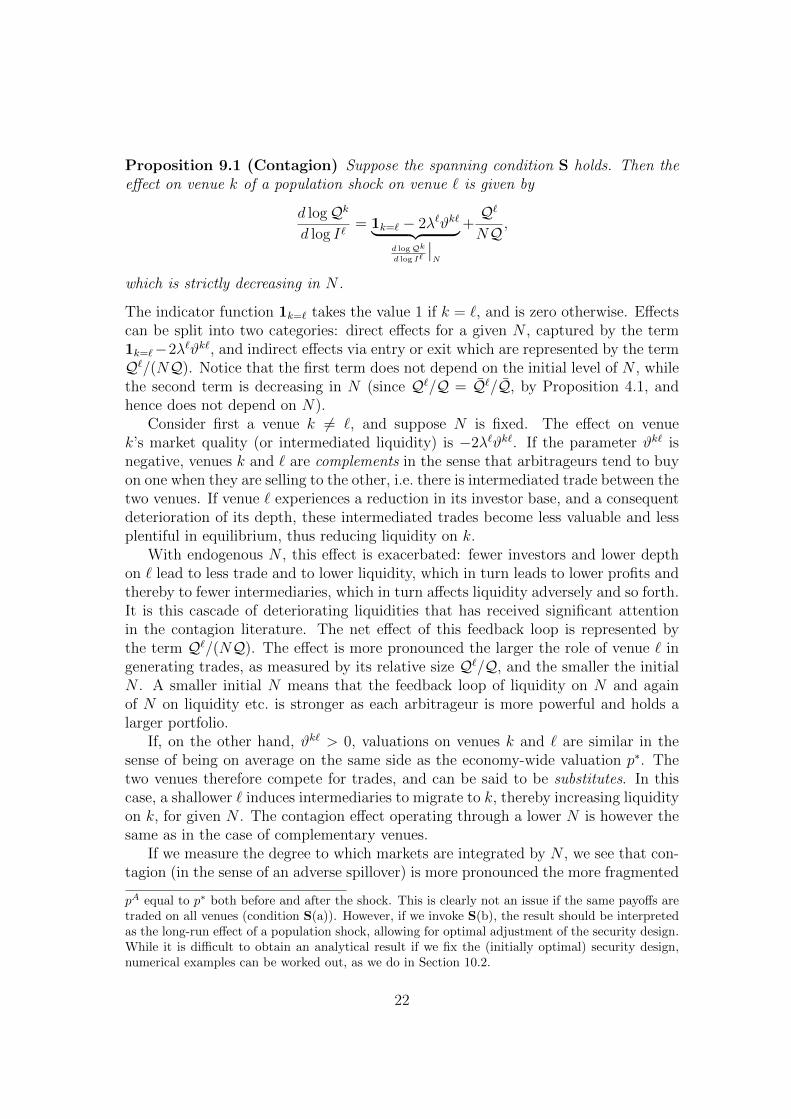
Proposition 9.1 (Contagion) Suppose the spanning condition S holds. Then theeffect on venue k of a population shock on venue ` is given by

d logQk

d log I`= 1k=` − 2λ`ϑk`︸ ︷︷ ︸

d logQkd log I`

∣∣N

+Q`

NQ,

which is strictly decreasing in N .

The indicator function 1k=` takes the value 1 if k = `, and is zero otherwise. Effectscan be split into two categories: direct effects for a given N , captured by the term1k=`−2λ`ϑk`, and indirect effects via entry or exit which are represented by the termQ`/(NQ). Notice that the first term does not depend on the initial level of N , whilethe second term is decreasing in N (since Q`/Q = Q`/Q, by Proposition 4.1, andhence does not depend on N).

Consider first a venue k 6= `, and suppose N is fixed. The effect on venuek’s market quality (or intermediated liquidity) is −2λ`ϑk`. If the parameter ϑk` isnegative, venues k and ` are complements in the sense that arbitrageurs tend to buyon one when they are selling to the other, i.e. there is intermediated trade between thetwo venues. If venue ` experiences a reduction in its investor base, and a consequentdeterioration of its depth, these intermediated trades become less valuable and lessplentiful in equilibrium, thus reducing liquidity on k.

With endogenous N , this effect is exacerbated: fewer investors and lower depthon ` lead to less trade and to lower liquidity, which in turn leads to lower profits andthereby to fewer intermediaries, which in turn affects liquidity adversely and so forth.It is this cascade of deteriorating liquidities that has received significant attentionin the contagion literature. The net effect of this feedback loop is represented bythe term Q`/(NQ). The effect is more pronounced the larger the role of venue ` ingenerating trades, as measured by its relative size Q`/Q, and the smaller the initialN . A smaller initial N means that the feedback loop of liquidity on N and againof N on liquidity etc. is stronger as each arbitrageur is more powerful and holds alarger portfolio.

If, on the other hand, ϑk` > 0, valuations on venues k and ` are similar in thesense of being on average on the same side as the economy-wide valuation p∗. Thetwo venues therefore compete for trades, and can be said to be substitutes. In thiscase, a shallower ` induces intermediaries to migrate to k, thereby increasing liquidityon k, for given N . The contagion effect operating through a lower N is however thesame as in the case of complementary venues.

If we measure the degree to which markets are integrated by N , we see that con-tagion (in the sense of an adverse spillover) is more pronounced the more fragmented

pA equal to p∗ both before and after the shock. This is clearly not an issue if the same payoffs aretraded on all venues (condition S(a)). However, if we invoke S(b), the result should be interpretedas the long-run effect of a population shock, allowing for optimal adjustment of the security design.While it is difficult to obtain an analytical result if we fix the (initially optimal) security design,numerical examples can be worked out, as we do in Section 10.2.

22

markets are. More precisely, the derivative in Proposition 9.1 is strictly decreasingin N , and is minimized as N goes to infinity and perfect integration is achieved. Ifk and ` are substitutes, this minimized value is negative; in this case the spillover ofa negative shock is actually benign.

Now consider the effect of a population shock on venue ` on its own liquidity. Forfixed N , this effect is given by (1− 2λ`). If λ` is small, this has the straightforwardinterpretation of the direct loss of liquidity due to the flight of investors. This iscompounded by the consequent flight of intermediaries in the same way as for therest of the economy. If λ` is non-negligible, however, there is a countervailing effect.Indeed, if λ` > 1/2, Q` actually increases when the population on ` falls, for givenN . This might at first appear odd, but the effect stems from the endogenous natureof Walrasian prices. Fewer investors on venue ` lower the depth of venue `, andeverything else constant, liquidity is lower. But the smaller size of this clientele alsomeans that it will now play a less prominent role in the determination of the economy-wide valuation p∗. The valuation p∗ will become more dissimilar from p`, therebyincreasing the potential gains from trade between ` and the rest of the economy,stimulating intermediated trades and increasing liquidity on `. If λ` > 1/2, thiseffect is strong enough to compensate for the loss of depth, before accounting for theknock-on effect on the number of intermediaries.

Evidently, in an economy with many venues, loss of liquidity is more likely togo hand in hand with a decline in the number of active investors. But there mightbe situations where a dominant venue optimally limits or rations participants. Itmay be that the arrival of more (identical) investors can hurt local liquidity. Theconverse implication is that liquidity can suffer on a venue that experiences a rise inits investor population while substitute venues at the same time benefit from higherliquidity. These examples show that there is a clear externality in our economy thatcan go in either direction.

For k 6= `, assuming that λ` < 1/2, it is easy to verify that

d logQk

d logQ`> 1 iff 2λ`(1− ϑk`) > 1 (12)

for the population-type shocks considered above. Thus, if ` is large in terms ofrelative depth, and k is sufficiently complementary with respect to `, a liquidityshock on ` has an even bigger impact on k than on ` itself. This is an illustration ofthe dictum that “when Russia sneezes, Brazil catches a cold.”

What is the effect on asset prices of a liquidity shock? It is instructive to considerthe case where the same assets trade on all venues so that price comparisons arestraightforward. Accordingly, we assume that dk = d, all k. Then q∗ := E[dp∗] is theasset price vector implied by the hypothetical complete-markets state-price deflatorfor the entire integrated economy.

Proposition 9.2 Suppose dk = d, for all k ∈ K. Then

∂qk

∂I`=

N

1 +N

λ`

I`(q` − q∗), k ∈ K.

23

Thus, if venue ` in isolation values assets more highly than the economy as a whole(q` > q∗), an adverse participation shock on ` depresses asset prices worldwide. Thisis because the tendency of venue ` to pull up asset prices, via intermediated trades,is reduced when its weight in the world economy is lower. Quite naturally, the effectis more pronounced the greater the degree of intermediation.

10 Examples of Contagious Illiquidity

In this section we illustrate how our framework can be used to understand the diffu-sion of liquidity shocks in a number of recent market events.

10.1 Trading Halt on the LSE

The UK FTSE stock market basically consists of the London Stock Exchange (LSE)as the main venue with around 60% of trading volume for FTSE-100 stocks, withBATS, Chi-X and Turquoise as the main MTFs.18 Since these venues trade a largecommon set of securities, one could reasonably view them as being competing venues,or substitutes. On Thursday 26th of November 2009, the LSE halted trading at 10:33due to a server error, placing all order books into auction mode until trading resumedat 14:00. If these venues were strong substitutes, our model would predict that anegative liquidity shock on the LSE would lead to higher liquidity on the MTFs.But the opposite happened. Liquidity dried up immediately on all the MTFs andrecovered only on the dot at 14:00 (see Intelligent Financial Systems (2009)).

Our model suggests that these markets should instead be understood as comple-ments, with arbitrageurs typically buying on one and selling on the other. By Propo-sition 9.1, an adverse shock to ILSE has a negative impact on the liquidity of an MTFif and only if 2λLSEϑLSE,MTF < QLSE

NQ . So all trading venues that are either weakenough substitutes or complements of the LSE would have their liquidity negativelyaffected by a liquidity shock to the LSE. In fact, (12) tells us that the impact on anMTF would be more pronounced than on the LSE itself if 2λLSE(1−ϑLSE,MTF ) > 1(we can safely assume that λLSE < 1/2). This condition is more likely to be satisfiedthe larger the relative weight of the LSE in pricing the true value of stocks, and thegreater the degree of complementarity. It would be an interesting empirical exerciseto estimate these numbers.

10.2 CDO Boom and Bust

Consider the CDO mechanism. The profit to intermediaries from structuring andmarketing CDOs ultimately stems from the fact that the tranched cash flows can besold for more than the procurement cost of the cash flows from credit, such as loansand mortgages.

18BATS acquired Chi-X in 2011. They were separate entities at the time of the trading halt onthe LSE.

24

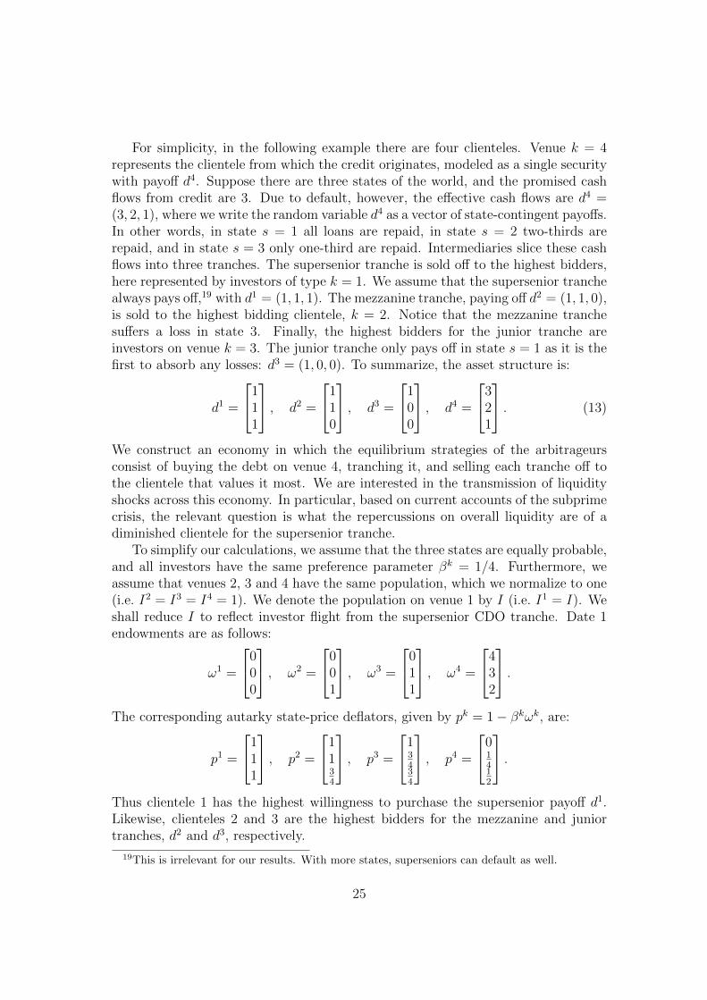
For simplicity, in the following example there are four clienteles. Venue k = 4represents the clientele from which the credit originates, modeled as a single securitywith payoff d4. Suppose there are three states of the world, and the promised cashflows from credit are 3. Due to default, however, the effective cash flows are d4 =(3, 2, 1), where we write the random variable d4 as a vector of state-contingent payoffs.In other words, in state s = 1 all loans are repaid, in state s = 2 two-thirds arerepaid, and in state s = 3 only one-third are repaid. Intermediaries slice these cashflows into three tranches. The supersenior tranche is sold off to the highest bidders,here represented by investors of type k = 1. We assume that the supersenior tranchealways pays off,19 with d1 = (1, 1, 1). The mezzanine tranche, paying off d2 = (1, 1, 0),is sold to the highest bidding clientele, k = 2. Notice that the mezzanine tranchesuffers a loss in state 3. Finally, the highest bidders for the junior tranche areinvestors on venue k = 3. The junior tranche only pays off in state s = 1 as it is thefirst to absorb any losses: d3 = (1, 0, 0). To summarize, the asset structure is:

d1 =

111

, d2 =

110

, d3 =

100

, d4 =

321

. (13)

We construct an economy in which the equilibrium strategies of the arbitrageursconsist of buying the debt on venue 4, tranching it, and selling each tranche off tothe clientele that values it most. We are interested in the transmission of liquidityshocks across this economy. In particular, based on current accounts of the subprimecrisis, the relevant question is what the repercussions on overall liquidity are of adiminished clientele for the supersenior tranche.

To simplify our calculations, we assume that the three states are equally probable,and all investors have the same preference parameter βk = 1/4. Furthermore, weassume that venues 2, 3 and 4 have the same population, which we normalize to one(i.e. I2 = I3 = I4 = 1). We denote the population on venue 1 by I (i.e. I1 = I). Weshall reduce I to reflect investor flight from the supersenior CDO tranche. Date 1endowments are as follows:

ω1 =

000

, ω2 =

001

, ω3 =

011

, ω4 =

432

.The corresponding autarky state-price deflators, given by pk = 1− βkωk, are:

p1 =

111

, p2 =

1134

, p3 =

13434

, p4 =

01412

.Thus clientele 1 has the highest willingness to purchase the supersenior payoff d1.Likewise, clienteles 2 and 3 are the highest bidders for the mezzanine and juniortranches, d2 and d3, respectively.

19This is irrelevant for our results. With more states, superseniors can default as well.

25

To understand the rationale for the CDO structure, consider first the benchmarkcase in which I = 1. Then the complete-markets Walrasian state-price deflator forthe integrated economy, p∗, is 3/4 in all three states. It is easy to check that the assetstructure (13) is the optimal security design, i.e. tranching is optimal for arbitrageurs.For every unit of d4 that arbitrageurs buy, they sell one unit each of the tranches d1,d2 and d3. The arbitrageurs’ valuation pA is equal to p∗.

Compare this, for instance, to the case in which a pass-through security is soldto all investors. Then the asset structure is (3, 2, 1) on all venues. The arbitrageurs’valuation is the same as above and equal to p∗. For every unit that arbitrageurs buyon venue 4, they sell 6/14, 5/14 and 3/14 units on venues 1, 2 and 3, respectively.Maximal market quality, Qk, is unchanged for venue 4 but is lower for the othervenues. The equilibrium level of intermediation is lower as well, leading to lowermarket quality, liquidity and welfare on all four venues.

While the CDO structure is optimal for I = 1, it is not so for other values ofI. In particular, we are interested in what happens if appetite for the superseniortranche diminishes, given this CDO structure. For I 6= 1, the spanning propertyS fails, which means that we cannot use the convenient condition pA = p∗. Thefollowing can be verified to be a Lagrange multiplier for the arbitrageurs’ first-orderconditions, and therefore a valid state-price deflator:

pA =3

17I + 3

4I + 14I + 19I − 4

,provided I ≥ 4/9, which we will henceforth assume.20 Equilibrium arbitrageur sup-plies are:

y1,n = y2,n = y3,n = −y4,n =1

1 +N· 20I

17I + 3.

Thus the pattern of trade is the same as in the benchmark case of I = 1. Thesetrades are simply scaled down as I falls. Notice that arbitrageur trades are exactlyoffsetting, so that

∑k y

k,ndk = 0. Equilibrium asset prices are given by:

q1 = 1− N1+N

517I+3

, q2 = 23− N

1+N10I

3(17I+3),

q3 = 13− N

1+N5I

3(17I+3), q4 = 1

3+ N

1+N70I

3(17I+3).

Maximal economy-wide market quality is

Q =100I

3(17I + 3).

As I falls, so does Q. This means that, even for fixed N , overall market qualityor liquidity Q, which is given by ( N

1+N )2Q, falls. In fact, it can be verified that the

20The results are less clear-cut when I falls below 4/9. This is because there are not enoughinvestors to absorb consumption in state 3, so it ends up in the hands of the arbitrageurs. Thenour assumption that arbitrageurs only care about consumption at date 0, which is fairly innocuousas long as the asset structure does not deviate too far from one that satisfies S, starts to matter.

26

same is true for the liquidity of tranches 2 and 3, and the liquidity of the underlyingdebt. Moreover, as I falls, intermediaries start going out of business, with N givenby rd(

√c−1L − 1). This exacerbates the drying up of liquidity.

Figures 1 and 2 illustrate the effects on liquidity and intermediation of a changein I, both above and below 1, for c = .001. That there is contagion is evident: as

Figure 1: Overall liquidity, Q, as a function of I

the natural clientele for the supersenior tranche is eroded, the entire CDO marketseizes up. A 50% decline in the size of this clientele (starting from I = 1) causesoverall liquidity to decline by more than 13%. This effect aggregates the impact ofa change in I on relative depths, on shadow prices pA, as well as on N . The plotsfor the liquidity of tranches 2 and 3, and for the liquidity of the securitized debt, aresimilar to that for overall liquidity.

During the boom phase, before doubts about the creditworthiness of CDOs andrelated products became prevalent, demand for tranches was in part fueled by thequest for yield in a low interest rate environment. In our model, the CDO mechanismleads to lower prices of the various tranches than would have obtained in its absence(i.e. qk < qk, k = 1, 2, 3). In other words, the CDOs allow the credit and moneymarkets to deliver higher yields. Likewise, the CDO mechanism allows debtors toborrow at a more attractive rate (q4 > q4).

Everything else constant, higher demand for the supersenior tranche leads to

27

Figure 2: Equilibrium Number of Arbitrageurs, N , as a function of I

higher supersenior prices,21 as well as higher prices for the underlying securitizeddebt. Concurrently, prices for the other tranches fall – and yields rise – since theseinvestors find more counterparties for their trades. And if on the contrary demandfor the supersenior tranche wanes, these effects are reversed: prices for tranches 2and 3 rise and the corresponding yields fall as arbitrageurs are forced to reduce theirshorts and buy back those tranches.

The crisis events unfolding in the credit markets from Summer 2007 onwardscannot be fully captured by this simple version of our model. Contrary to ourassumptions here, banks in the real world did have their own capital and used it tokeep the supersenior tranches when they found no buyers for them. They went onstructuring CDOs and selling the remaining lower graded tranches off, pocketing the“arbitrage” profits (they were arbitrage trades for the structuring desks, who sold thesupersenior tranches to the treasury department of the same organization, but notfor the intermediary as a whole). This overextension into CDOs then became plainwhen an “unexpected” state was realized wherein the supersenior tranches were nolonger perceived to pay back their face value. More elaborate versions of our modelcan be constructed to allow for arbitrageur capital and for default, but this is beyondthe scope of this paper.

21One can check that this is true in spite of the countervailing effect of higher N .

28

10.3 Japan-US in the Early 1990s

As a further illustration of contagion, this time of the macro type, consider theliquidity shock emanating from Japan at the end of the 1980s and beginning of the1990s, as documented for example by Peek and Rosengren (1997). We can interpretthis shock as a drop in the Japanese local investor base. While Japan was a majorfinancial power, it is safe to assume that it did not account for more than half ofthe world’s financial depth. Given that the flow of capital was from Japan to theUS, Japan and the US were complements, and on average asset prices were higherin Japan than in the rest of the world. The adverse shock to Japanese liquiditydepressed stock prices in Japan. The authors documented that the result of thisliquidity shock was a sharp decline in Japanese investment in the US, which inturn adversely affected liquidity in the US, an instance of contagion along the linessuggested by our model (in particular, Proposition 9.2).

11 Relationship to the Literature

Despite the recent interest in liquidity fragmentation, the increasing complexity ofstructured products exploiting segmentation, the growth of latency arbitrage byHFTs, and the need for a rigorous analysis of the forces of market integration forregulatory purposes, academic research on these subjects is still in its infancy. Whilethere is a vast literature studying market liquidity directly or indirectly, market qual-ity in general remains a bit nebulous. We are not aware of any papers that definemarket quality or liquidity via an explicit metric that itself has a clear welfare mean-ing, or that relate this definition to the different attributes of liquidity, such as depth,bid-ask spreads or volume.

Traditionally, liquidity has been studied empirically in single-asset models (see,for example, the papers cited in Chordia et al. (2000)), with little attention given tomulti-asset liquidity, common factors, liquidity substitutes and so forth. Recently,however, a few papers have started to address this omission, among them Chor-dia et al. (2000), Hasbrouck and Seppi (2001) and Korajczyk and Sadka (2008).Similarly, the effect of multiple trading venues on liquidity has not been studiedextensively. While many papers compare liquidity metrics such as bid-ask spreadson an ECN with those on an exchange, with both being analyzed in isolation, fewerstudy the effects on liquidity of the interaction between ECNs and exchanges. In thelatter camp are Hendershott and Mendelson (2000), Weston (2002), Foucault andMenkveld (2008) and Biais et al. (2010), who find that in general the growth of elec-tronic competitors has had a positive impact on bid-ask spreads in the underlyingmarkets. None of these papers explicitly studies the effects of cross-venue trades,however, with the exception of Karolyi et al. (2012) who argue that during periodsof market stress, commonalities appear that are due to the crisis-induced trades bycross-market arbitrageurs, a theme that we also explore in this paper.

There is a growing empirical literature in support of segmentation and clientele

29

pricing in asset markets; see Rahi and Zigrand (2009) for a discussion of this lit-erature. That there are arbitrage opportunities across markets, often fleeting, iswell-known. Most such opportunities occur between less well-researched or tailoredsecurities, between related derivatives, or between derivatives and replicating strate-gies of varying degrees of sophistication. But even bids and asks for liquid Nasdaqstocks cross occasionally across trading venues (i.e. the bid on one venue is higherthan the ask on another).22 Garvey and Murphy (2006) for instance show that intheir sample, consisting of the 10 most traded stocks on Nasdaq in addition to the10 stocks with the largest market caps, crosses occur about .5% of the time.

A key ingredient of our theoretical model is the close connection of liquidity toarbitrage activity. This connection has been documented empirically by Hu et al.(2012) in the market for US Treasuries. They find that during market crises, shortageof arbitrage capital allows yields to move more freely relative to the curve, resultingin more “noise” in prices and hence in “less liquid” markets.

In terms of theoretical work, not much has been done on multi-asset liquidity.Gromb and Vayanos (2009) study the provision of liquidity by arbitrageurs in asegmented markets setting, with arbitrage opportunities arising across pairs of assetstraded on different market segments, and a continuum of competitive arbitrageurswho face a separate margin constraint in each asset. Their main concern is the effecton liquidity (defined as depth) of this financial constraint, which is the source ofthe limits to arbitrage in their model. In our paper, on the other hand, arbitrage islimited due to a cost of entering the arbitraging business, and imperfect competitionamong arbitrageurs. Our framework also allows for an arbitrary asset structureacross trading venues. Brunnermeier and Pedersen (2009) model liquidity needs asarising from the asynchronous arrival of investors. Like Gromb and Vayanos (2009),they study the link between the margin constraints faced by speculators and theliquidity they provide. Fernando (2003) models “liquidity shocks” as additive shocksthat affect investors’ marginal valuations of risky assets. His main interests are theprice effects of idiosyncratic versus systematic liquidity shocks and the impact ofliquidity shocks to one asset on prices of other assets. Cespa and Foucault (2012)model liquidity spillovers across assets as arising through an informational channelwhereby a less liquid market for one security carries less information, which affectsthe information set of dealers in other markets and hence the liquidity provided bythese dealers.

Our analysis builds on our earlier work in Rahi and Zigrand (2009, 2013). We usesome results from these papers, in particular on the characterization of equilibrium.

22In 2005, 42% of trades in Nasdaq stocks occurred on Nasdaq with the remaining 58% occurringin non-linked market centers. Note that the observed crosses are the outcomes of segmentation leftunarbitraged by intermediaries: absent arbitrageurs many more crosses would be observed.

30

12 Conclusion

In this paper we study financial market quality in a world in which trading is frag-mented across multiple venues or platforms. We define an intuitive metric of marketquality that captures the true economic meaning of the liquidity provided by inter-mediaries, namely the extent to which gains from trade are realized through inter-mediation. This metric can be expressed in terms of the real resources gained byinvestors as a result of this intermediation. It can be applied to one security tradedon a single platform, but its strength lies in being able to aggregate liquidity acrossmultiple securities and trading venues.

Standard liquidity metrics rely on a particular choice of both the metric, thatis seldom explicitly welfare-grounded (such as bid-ask spreads or depth), and of asmall number of securities, thereby ignoring substitutes as well as the overall marketequilibrium. Our market quality metric does not suffer from such shortcomingsand “sees through” the structure of markets to provide a measure that captures themagnitude of welfare-improving transactions realized in equilibrium. Our metric alsohas a clear relationship to volume, depth, intermediation costs and the like.

We explicitly model the role of profit-maximizing, liquidity-providing interme-diaries who link markets together. The number of intermediaries is part of theequilibrium and is both influenced by market quality, and influences it in turn. Theintermediation can be functional or geographic, and can encompass a variety oftrading activities, from arbitrage between derivatives and the underlying markets tothe huge industry of latency arbitrage across multiple lit and dark trading venuesthat has been in the regulatory limelight recently. We also allow intermediaries tointroduce new securities, and we show that security design improves overall marketquality, though local market quality may decline on some venues. The intermediariesform endogenous links across markets, and the strength of these linkages determinesthe transmission of liquidity shocks through the system.

We illustrate how in a number of recent market events the diffusion of liquidityshocks can be understood through the lens of interconnected markets provided bythe setup in this paper. For instance, the advent of HFTs offering market makingservices across exchanges and MTFs suggests that some of these MTFs are comple-ments rather than substitutes of the main venues in the sense that liquidity on onerelies positively on liquidity on the others. The outage on the London Stock Ex-change on the 26th of November 2009 rippled through the network of interconnectedmarkets and brought liquidity across all related MTFs crashing down, even thoughthe alternative venues were supposed to pick up the liquidity lost on the LSE. Ourmodel suggests that most of the trades on the MTFs were arbitrage trades by HFTsbetween these venues and the LSE.

We show that the impact of a local shock on the size of the intermediation sectorhas a feedback multiplier effect on market quality – for instance, a negative liquid-ity shock forces some intermediaries to exit, thus reducing liquidity, inducing moreintermediaries to exit, and so forth. We illustrate this with an example of conta-

31

gion in CDO markets, wherein a demand shock to one tranche reverberates throughthe entire system, impacting the liquidity of all the other tranches. By interpretingtrading venues as countries, our setup can also shed light on cross-border investmentflows following a shock in one country, as in the case of the bursting of the Japanesebubble and its effect on the US stock market.

Appendix

In the Appendix we adopt matrix notation in order to simplify the proofs. Werepresent asset payoffs dk by the S×Jk matrix Rk whose j’th column lists the state-by-state payoffs of the j’th asset. The set of traded payoffs Mk is then the columnspace of Rk.

Let Π be the diagonal matrix whose diagonal elements are the probabilities ofthe states, π1, . . . , πS. A state-price deflator for (q, R) is a vector p ∈ RS such thatq = R>Πp.23 In other words, state-price deflators can be viewed as vectors insteadof random variables. Similarly, the expectation E[xy] can be written as x>Πy, wherethe random variables x and y are viewed as vectors in RS. In our finite-dimensionalsetting, the inner product space L2 is the space RS endowed with the inner product〈x, y〉2 := x>Πy. Then xMk = P kx, where P k is the orthogonal projection operator

in L2 onto Mk, given by the idempotent matrix P k := Rk(Rk>ΠRk)−1Rk>Π. Anexplicit derivation of P k can be found in Rahi and Zigrand (2009). P k depends on

Rk only through the span Mk. The L2-norm of x ∈ RS is ‖x‖2 := (x>Πx)12 .

In this notation, market quality on venue k is

Qk =1

βk‖P k(pk − pk)‖2

2.

Proof of Proposition 2.1 The proof is adapted from arguments in Chen andKnez (1995). Let the asset payoff matrix be R with marketed subspace M andcorresponding projection matrix P .

The first statement says that P (p − p′) = 0 if and only if R>Π(p − p′) = 0. IfP (p−p′) = 0, then R>ΠP (p−p′) = 0. But R>ΠP = R>Π, so that R>Π(p−p′) = 0.Conversely, R>Π(p− p′) = 0 implies that (p− p′) ∈M⊥. Hence P (p− p′) = 0.

Next we prove the third statement. Consider a payoff z, not necessarily inM . Themispricing of z using Pp versus Pp′ is m(z) := z>ΠP (p−p′). Since ΠP = P>ΠP , bythe Cauchy-Schwartz inequality we have m(z) ≤ ‖Pz‖2‖P (p− p′)‖2; equality occursif and only if Pz and P (p− p′) are collinear. It follows that

‖P (p− p′)‖2 = maxz:‖Pz‖2=1

z>ΠP (p− p′). (14)

23The symbol > denotes “transpose.” We adopt the convention of taking all vectors to be columnvectors by default, unless transposed.

32

For the second statement, consider a payoff z ∈ M . Then z = Rθ for some θ ∈ RJ .Using again the fact that R>ΠP = R>Π, we see that m(z) = z>Π(p − p′). Hence,(14) can be written as

‖P (p− p′)‖2 = maxz∈M :‖z‖2=1

z>Π(p− p′).

Proof of Proposition 5.1

Qk =1

βk‖P k(pk − pk)‖2

2

=1

βk(pk − pk)>P k>ΠP k(pk − pk)

=1

βk(pk − pk)>ΠRk(Rk>ΠRk)−1︸ ︷︷ ︸

bk>

Rk>Π(pk − pk)︸ ︷︷ ︸qk−qk

.

Proof of Proposition 5.3 Using (3), we have

qk =1

1 +Nqk +

N

1 +Nq∗,

where q∗ = E[dp∗]. It follows that qk − qk = N(qk − q∗). From Proposition 5.2,Qkj = Nθkj (q

kj − q∗j ) = Nykj (qkj − q∗j ). Since the same assets trade on all venues,

arbitrageur holdings of any asset, aggregated across all venues, must be zero, i.e.∑k y

k = 0. Hence, Qj = N∑

k ykj q

kj .

Proof of Proposition 9.1 In order to calculate the effect of a proportional changein I`, d log I`, it is convenient to write the population of venue ` as αI`, with corre-sponding depth α/β`, and compute derivatives with respect to α evaluated at α = 1.Using (9), we can write Qk as a function of α, pA and N :

Qk(α, pA(α), N(α)) =αk

βk

(N

1 +N

)2

‖P k(pk − pA)‖22

=αk

βk

(N

1 +N

)2

(pk − pA)>ΠP k(pk − pA),

where αk = α for k = `, and αk = 1 for k 6= `. The total derivative of Qk withrespect to α is

dQk

dα=∂Qk

∂α+∂Qk

∂pA· pA′(α)︸ ︷︷ ︸

dQkdα

∣∣∣N

+∂Qk

∂NN ′(α). (15)

33

Noting that

pA(α) =

αβ`p` +

∑k 6=`

1βkpk

αβ`

+∑

k 6=`1βk

,

we have

∂Qk

∂α= Q`1k=`

∂Qk

∂pA= − 2

βk

(N

1 +N

)2

ΠP k(pk − pA)

pA′(α) = λ`(p` − pA) =

βkλk

β`(p` − pA), (16)

where all the derivatives are evaluated at α = 1. Hence the effect on Qk for given Nis

dQk

dα

∣∣∣∣N

= Q`1k=` −2λk

β`

(N

1 +N

)2

ϕk`, (17)

whereϕk` := (pk − pA)>ΠP k(p` − pA).

We now solve for N ′(α). With free entry, Q = cN2 (Proposition 4.3). Therefore, thefunction N(α) is defined by the identity∑

k

Qk(α, pA(α), N(α))− c[N(α)]2 ≡ 0.

Implicit differentiation gives us

N ′(α) =

∑kdQkdα

∣∣∣N

2cN −∑

k∂Qk∂N

.

Now∂Qk

∂N=

2

N(1 +N)Qk, (18)

so that ∑k

∂Qk

∂N=

2

N(1 +N)Q =

2cN

1 +N,

where we have once again used the result that Q = cN2.Under the spanning condition S, either P k = P or P k(pk − pA) = pk − pA. In

both cases∑

k λkϕk` = 0, since pA = p∗. Therefore, from (17),

∑k

dQk

dI`

∣∣∣∣N

= Q`.

34

Altogether, this yields

N ′(α) =(1 +N)Q`

2cN2=

(1 +N)Q`

2Q. (19)

Substituting (17), (18) and (19) into (15) gives us

dQk

dα= Q`1k=` −

2λk

β`

(N

1 +N

)2

ϕk` +QkQ`

NQ.

Dividing through by Qk we get the desired result (note that ϑk` = ϕk`

ϕk,k).

Proof of Proposition 9.2 Let Rk = R, all k. Then, using (3),

qk = R>Πpk

= R>Π

(1

1 +Npk +

N

1 +NpA).

Therefore, from (16),

∂qk

∂d log I`=

N

1 +Nλ`R>Π(p` − pA).

Moreover, since condition S(a) is satisfied, we have pA = p∗. This yields the desiredresult.

References

Beddington, J., Bond, P., Cliff, D., Houstoun, K., Linton, O., Goodhart, C., andZigrand, J.-P. (2013). The Future of Computer Trading in Financial Markets: AnInternational Perspective. Foresight.

Biais, B., Bisiere, C., and Spatt, C. (2010). Imperfect competition in financial mar-kets: An empirical study of Island and Nasdaq. Management Science, 56(12):2237–2250.

Brunnermeier, M. and Pedersen, L. (2009). Market liquidity and funding liquidity.Review of Financial Studies, 22(6):2201–2199.

Cespa, G. and Foucault, T. (2012). Illiquidity contagion and liquidity crashes. Work-ing Paper.

CFTC and SEC (2010). Findings regarding the market events of May 6, 2010. Reportof the Staffs of the CFTC and SEC to the Joint Advisory Committee on EmergingRegulatory Issues.

35

Chen, Z. and Knez, P. J. (1995). Measurement of market integration and arbitrage.Review of Financial Studies, 8(2):287–325.

Chordia, T., Roll, R., and Subrahmanyam, A. (2000). Commonality in liquidity.Journal of Financial Economics, 56(1):3–28.

Donefer, B. S. (2008). Risk management and electronic trading. Mimeo, FIX ProtocolConference.

Fernando, C. S. (2003). Commonality in liquidity: Transmission of liquidity shocksacross investors and securities. Journal of Financial Intermediation, 12:233–254.

Foucault, T. and Menkveld, A. J. (2008). Competition for order flow and smartorder routing systems. Journal of Finance, 63:119–158.

Garvey, R. and Murphy, A. (2006). Crossed markets: Arbitrage opportunities inNasdaq stocks. The Journal of Alternative Investments, 9(2):46–58.

Gromb, D. and Vayanos, D. (2009). Financially constrained arbitrage and cross-market contagion. Mimeo, London School of Economics.

Hasbrouck, J. and Seppi, D. (2001). Common factors in prices, order flows andliquidity. Journal of Financial Economics, 59(3):383–411.

Hendershott, T. and Mendelson, H. (2000). Crossing networks and dealer markets:Competition and efficiency. Journal of Finance, 55:1–40.

Hu, X., Pan, J., and Wang, J. (2012). Noise as information for illiquidity. WorkingPaper.

Hunsader, E. (2010). Nanex flash crash summary report. Technical report, Nanex.http://www.nanex.net/FlashCrashFinal/FlashCrashSummary III.html.

Intelligent Financial Systems (2009). What was the impact of theLSE outage on Thurs 26th Nov 2009? LiquidMetrix Short Article,http://www.if5.com/LiquidMetrix/Articles/LM001.

Karolyi, G. A., Lee, K.-H., and van Dijk, M. A. (2012). Understanding commonalityin liquidity around the world. Journal of Financial Economics, 105(1):82–112.

Kearns, M., Kulesza, A., and Nevmyvaka, Y. (2010). Empirical limitations on high-frequency trading profitability. Journal of Trading, 5(4):50–62.

Korajczyk, R. and Sadka, R. (2008). Pricing the commonality across alternativemeasures of liquidity. Journal of Financial Economics, 87(1):45–72.

Peek, J. and Rosengren, E. S. (1997). The international transmission of financialshocks: The case of Japan. American Economic Review, 87(4):495–505.

36

Rahi, R. and Zigrand, J.-P. (2009). Strategic financial innovation in segmentedmarkets. Review of Financial Studies, 22(8):2941–2971.

Rahi, R. and Zigrand, J.-P. (2013). Walrasian foundations for equilibria in segmentedmarkets. Mimeo, London School of Economics.

Strasbourg, J. (2011). A wild ride to profits. Wall Street Journal.http://online.wsj.com/article/SB10001424053111904253204576510371408072058.html,accessed September 6, 2012.

Weston, J. (2002). Electronic communication networks and liquidity on the Nasdaq.Journal of Financial Services Research, 22(1&2):125–139.

37