Market Power: Monopoly and Monopsonynuriyildirim.weebly.com/uploads/5/9/9/7/59978521/ch10.pdfFernando & Yvonn Quijano Prepared by: Market Power: Monopoly and Monopsony E R 10 Copyright

Fernando & Yvonn Quijano

Prepared by:

Market Power: Monopoly and Monopsony

10

C H

A P

T E

R

Copyright © 2009 Pearson Education, Inc. Publishing as Prentice Hall • Microeconomics • Pindyck/Rubinfeld, 8e.

Ch

ap

ter

10

: M

ark

et

Po

we

r: M

on

op

oly

an

d M

on

op

so

ny

2 of 50 Copyright © 2009 Pearson Education, Inc. Publishing as Prentice Hall • Microeconomics • Pindyck/Rubinfeld, 8e.

CHAPTER 10 OUTLINE

10.1 Monopoly

10.2 Monopoly Power

10.3 Sources of Monopoly Power

10.4 The Social Costs of Monopoly Power

10.5 Monopsony

10.6 Monopsony Power

10.7 Limiting Market Power: The Antitrust Laws

Ch

ap

ter

10

: M

ark

et

Po

we

r: M

on

op

oly

an

d M

on

op

so

ny


● monopoly Market with only one seller.

● monopsony Market with only one buyer.

● market power Ability of a seller or buyer

to affect the price of a good.

Market Power: Monopoly and Monopsony

Ch

ap

ter

10

: M

ark

et

Po

we

r: M

on

op

oly

an

d M

on

op

so

ny


MONOPOLY 10.1

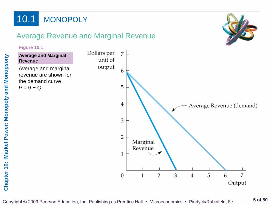
Average Revenue and Marginal Revenue

● marginal revenue Change in revenue

resulting from a one-unit increase in output.

TABLE 10.1 Total, Marginal, and Average Revenue

Total Marginal Average

Price (P) Quantity (Q) Revenue (R) Revenue (MR) Revenue (AR)

$6 0 $0 --- ---

5 1 5 $5 $5

4 2 8 3 4

3 3 9 1 3

2 4 8 -1 2

1 5 5 -3 1

Ch

ap

ter

10

: M

ark

et

Po

we

r: M

on

op

oly

an

d M

on

op

so

ny


MONOPOLY 10.1

Average Revenue and Marginal Revenue

Average and marginal

revenue are shown for

the demand curve

P = 6 − Q.

Average and Marginal

Revenue

Figure 10.1

Ch

ap

ter

10

: M

ark

et

Po

we

r: M

on

op

oly

an

d M

on

op

so

ny


MONOPOLY 10.1

The Monopolist’s Output Decision

Q* is the output level at which

MR = MC.

If the firm produces a smaller

output—say, Q1—it sacrifices

some profit because the extra

revenue that could be earned

from producing and selling the

units between Q1 and Q*

exceeds the cost of producing

them.

Similarly, expanding output from

Q* to Q2 would reduce profit

because the additional cost

would exceed the additional

revenue.

Profit Is Maximized When Marginal

Revenue Equals Marginal Cost

Figure 10.2

Ch

ap

ter

10

: M

ark

et

Po

we

r: M

on

op

oly

an

d M

on

op

so

ny


MONOPOLY 10.1

The Monopolist’s Output Decision

We can also see algebraically that Q* maximizes profit. Profit π is the

difference between revenue and cost, both of which depend on Q:

As Q is increased from zero, profit will increase until it reaches a

maximum and then begin to decrease. Thus the profit-maximizing

Q is such that the incremental profit resulting from a small increase

in Q is just zero (i.e., Δπ /ΔQ = 0). Then

But ΔR/ΔQ is marginal revenue and ΔC/ΔQ is marginal cost. Thus

the profit-maximizing condition is that

, or

Ch

ap

ter

10

: M

ark

et

Po

we

r: M

on

op

oly

an

d M

on

op

so

ny


MONOPOLY 10.1

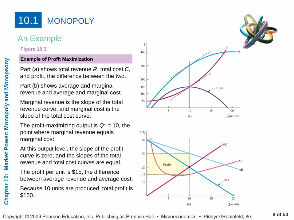
An Example

Part (a) shows total revenue R, total cost C,

and profit, the difference between the two.

Part (b) shows average and marginal

revenue and average and marginal cost.

Marginal revenue is the slope of the total

revenue curve, and marginal cost is the

slope of the total cost curve.

The profit-maximizing output is Q* = 10, the

point where marginal revenue equals

marginal cost.

At this output level, the slope of the profit

curve is zero, and the slopes of the total

revenue and total cost curves are equal.

The profit per unit is $15, the difference

between average revenue and average cost.

Because 10 units are produced, total profit is

$150.

Example of Profit Maximization

Figure 10.3

Ch

ap

ter

10

: M

ark

et

Po

we

r: M

on

op

oly

an

d M

on

op

so

ny


MONOPOLY 10.1

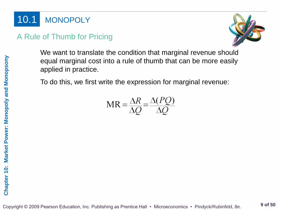
A Rule of Thumb for Pricing

We want to translate the condition that marginal revenue should

equal marginal cost into a rule of thumb that can be more easily

applied in practice.

To do this, we first write the expression for marginal revenue:

Ch

ap

ter

10

: M

ark

et

Po

we

r: M

on

op

oly

an

d M

on

op

so

ny


MONOPOLY 10.1


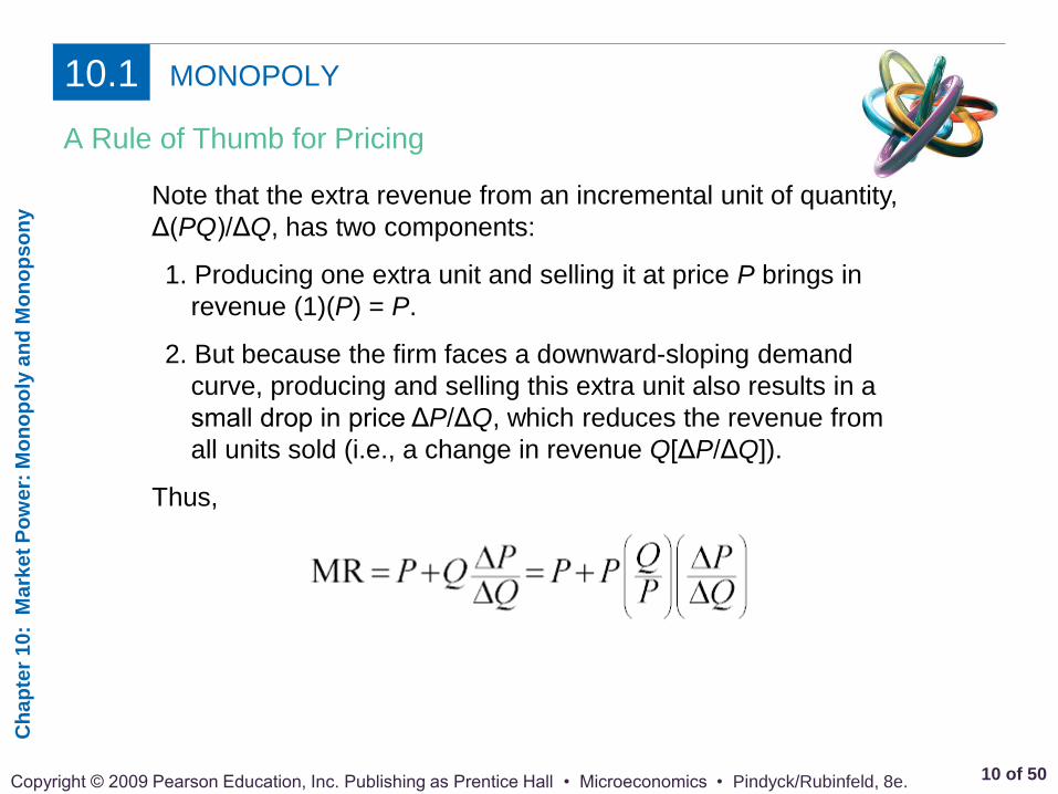
Note that the extra revenue from an incremental unit of quantity,

Δ(PQ)/ΔQ, has two components:

1. Producing one extra unit and selling it at price P brings in

revenue (1)(P) = P.

2. But because the firm faces a downward-sloping demand

curve, producing and selling this extra unit also results in a

small drop in price ΔP/ΔQ, which reduces the revenue from

all units sold (i.e., a change in revenue Q[ΔP/ΔQ]).

Thus,

Ch

ap

ter

10

: M

ark

et

Po

we

r: M

on

op

oly

an

d M

on

op

so

ny


MONOPOLY 10.1


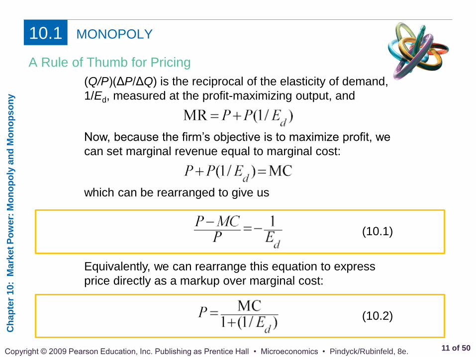
(Q/P)(ΔP/ΔQ) is the reciprocal of the elasticity of demand,

1/Ed, measured at the profit-maximizing output, and

Now, because the firm’s objective is to maximize profit, we

can set marginal revenue equal to marginal cost:

which can be rearranged to give us

(10.1)

Equivalently, we can rearrange this equation to express

price directly as a markup over marginal cost:

(10.2)

Ch

ap

ter

10

: M

ark

et

Po

we

r: M

on

op

oly

an

d M

on

op

so

ny


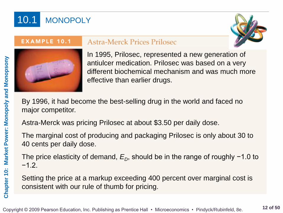
In 1995, Prilosec, represented a new generation of

antiulcer medication. Prilosec was based on a very

different biochemical mechanism and was much more

effective than earlier drugs.

By 1996, it had become the best-selling drug in the world and faced no

major competitor.

Astra-Merck was pricing Prilosec at about $3.50 per daily dose.

The marginal cost of producing and packaging Prilosec is only about 30 to

40 cents per daily dose.

The price elasticity of demand, ED, should be in the range of roughly −1.0 to

−1.2.

Setting the price at a markup exceeding 400 percent over marginal cost is

consistent with our rule of thumb for pricing.

MONOPOLY 10.1

Ch

ap

ter

10

: M

ark

et

Po

we

r: M

on

op

oly

an

d M

on

op

so

ny


MONOPOLY 10.1

Shifts in Demand

A monopolistic market has no supply curve.

The reason is that the monopolist’s output decision depends not only

on marginal cost but also on the shape of the demand curve.

Shifts in demand can lead to changes in price with no change in

output, changes in output with no change in price, or changes in both

price and output.

Ch

ap

ter

10

: M

ark

et

Po

we

r: M

on

op

oly

an

d M

on

op

so

ny


MONOPOLY 10.1

Shifts in Demand

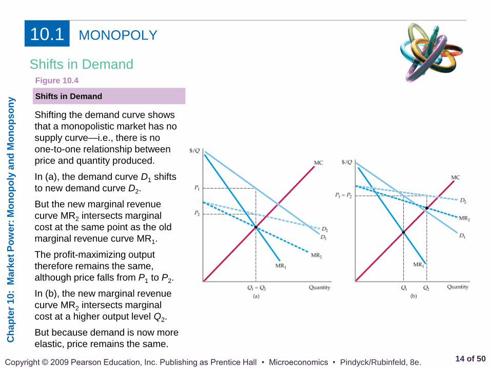
Shifting the demand curve shows

that a monopolistic market has no

supply curve—i.e., there is no

one-to-one relationship between

price and quantity produced.

In (a), the demand curve D1 shifts

to new demand curve D2.

But the new marginal revenue

curve MR2 intersects marginal

cost at the same point as the old

marginal revenue curve MR1.

The profit-maximizing output

therefore remains the same,

although price falls from P1 to P2.

In (b), the new marginal revenue

curve MR2 intersects marginal

cost at a higher output level Q2.

But because demand is now more

elastic, price remains the same.

Shifts in Demand

Figure 10.4

Ch

ap

ter

10

: M

ark

et

Po

we

r: M

on

op

oly

an

d M

on

op

so

ny


MONOPOLY 10.1

The Effect of a Tax

With a tax t per unit, the firm’s

effective marginal cost is

increased by the amount t to

MC + t.

In this example, the increase in

price ΔP is larger than the tax t.

Effect of Excise Tax on Monopolist

Figure 10.5

Suppose a specific tax of t dollars per unit is levied, so that the monopolist

must remit t dollars to the government for every unit it sells. If MC was the

firm’s original marginal cost, its optimal production decision is now given by

Ch

ap

ter

10

: M

ark

et

Po

we

r: M

on

op

oly

an

d M

on

op

so

ny


MONOPOLY 10.1

The Multiplant Firm

Suppose a firm has two plants. What should its total output be, and how

much of that output should each plant produce? We can find the answer

intuitively in two steps.

● Step 1. Whatever the total output, it should be divided between

the two plants so that marginal cost is the same in each plant.

Otherwise, the firm could reduce its costs and increase its profit

by reallocating production.

● Step 2. We know that total output must be such that marginal

revenue equals marginal cost. Otherwise, the firm could increase

its profit by raising or lowering total output.

Ch

ap

ter

10

: M

ark

et

Po

we

r: M

on

op

oly

an

d M

on

op

so

ny


MONOPOLY 10.1

The Multiplant Firm

We can also derive this result algebraically. Let Q1 and C1 be the output

and cost of production for Plant 1, Q2 and C2 be the output and cost of

production for Plant 2, and QT = Q1 + Q2 be total output. Then profit is

The firm should increase output from each plant until the incremental profit

from the last unit produced is zero. Start by setting incremental profit from

output at Plant 1 to zero:

Here Δ(PQT)/ΔQ1 is the revenue from producing and selling one more unit—

i.e., marginal revenue, MR, for all of the firm’s output.

Ch

ap

ter

10

: M

ark

et

Po

we

r: M

on

op

oly

an

d M

on

op

so

ny


MONOPOLY 10.1

The Multiplant Firm

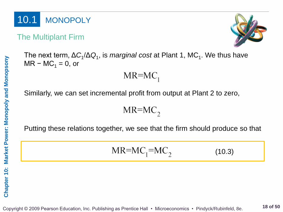
The next term, ΔC1/ΔQ1, is marginal cost at Plant 1, MC1. We thus have

MR − MC1 = 0, or

Similarly, we can set incremental profit from output at Plant 2 to zero,

Putting these relations together, we see that the firm should produce so that

(10.3)

Ch

ap

ter

10

: M

ark

et

Po

we

r: M

on

op

oly

an

d M

on

op

so

ny


MONOPOLY 10.1

The Multiplant Firm

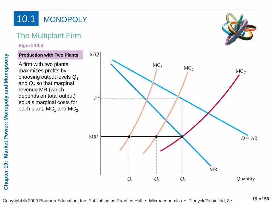
A firm with two plants

maximizes profits by

choosing output levels Q1

and Q2 so that marginal

revenue MR (which

depends on total output)

equals marginal costs for

each plant, MC1 and MC2.

Production with Two Plants

Figure 10.6

Ch

ap

ter

10

: M

ark

et

Po

we

r: M

on

op

oly

an

d M

on

op

so

ny


MONOPOLY POWER 10.2

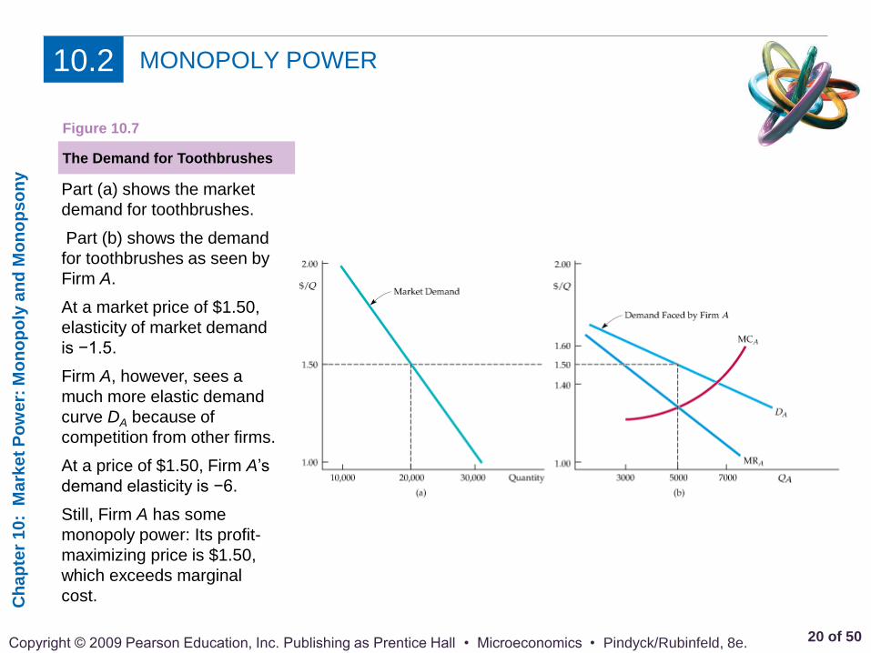
Part (a) shows the market

demand for toothbrushes.

Part (b) shows the demand

for toothbrushes as seen by

Firm A.

At a market price of $1.50,

elasticity of market demand

is −1.5.

Firm A, however, sees a

much more elastic demand

curve DA because of

competition from other firms.

At a price of $1.50, Firm A’s

demand elasticity is −6.

Still, Firm A has some

monopoly power: Its profit-

maximizing price is $1.50,

which exceeds marginal

cost.

The Demand for Toothbrushes

Figure 10.7

Ch

ap

ter

10

: M

ark

et

Po

we

r: M

on

op

oly

an

d M

on

op

so

ny


MONOPOLY POWER 10.2

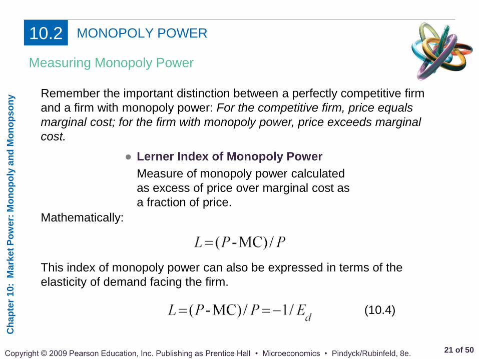
Remember the important distinction between a perfectly competitive firm

and a firm with monopoly power: For the competitive firm, price equals

marginal cost; for the firm with monopoly power, price exceeds marginal

cost.

Measuring Monopoly Power

● Lerner Index of Monopoly Power

Measure of monopoly power calculated

as excess of price over marginal cost as

a fraction of price.

Mathematically:

This index of monopoly power can also be expressed in terms of the

elasticity of demand facing the firm.

(10.4)

Ch

ap

ter

10

: M

ark

et

Po

we

r: M

on

op

oly

an

d M

on

op

so

ny


MONOPOLY POWER 10.2

The Rule of Thumb for Pricing

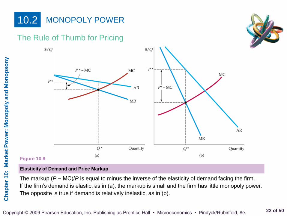
The markup (P − MC)/P is equal to minus the inverse of the elasticity of demand facing the firm.

If the firm’s demand is elastic, as in (a), the markup is small and the firm has little monopoly power.

The opposite is true if demand is relatively inelastic, as in (b).

Elasticity of Demand and Price Markup

Figure 10.8

Ch

ap

ter

10

: M

ark

et

Po

we

r: M

on

op

oly

an

d M

on

op

so

ny


MONOPOLY POWER 10.2

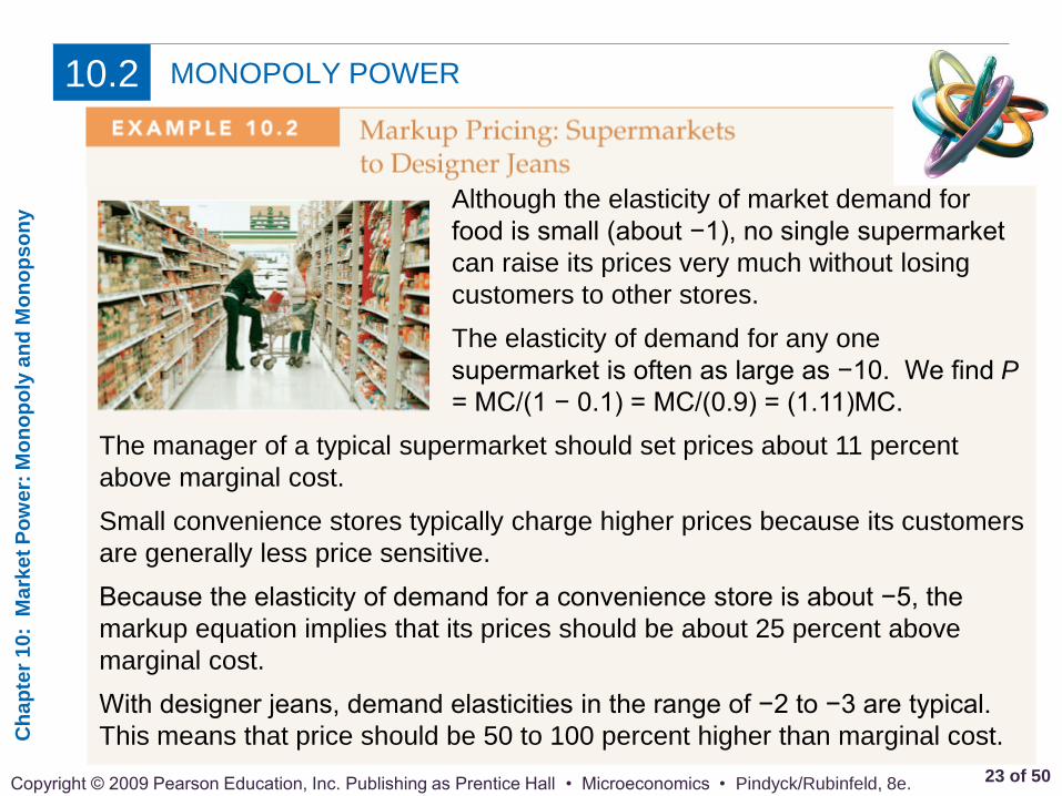
Although the elasticity of market demand for

food is small (about −1), no single supermarket

can raise its prices very much without losing

customers to other stores.

The elasticity of demand for any one

supermarket is often as large as −10. We find P

= MC/(1 − 0.1) = MC/(0.9) = (1.11)MC.

The manager of a typical supermarket should set prices about 11 percent

above marginal cost.

Small convenience stores typically charge higher prices because its customers

are generally less price sensitive.

Because the elasticity of demand for a convenience store is about −5, the

markup equation implies that its prices should be about 25 percent above

marginal cost.

With designer jeans, demand elasticities in the range of −2 to −3 are typical.

This means that price should be 50 to 100 percent higher than marginal cost.

Ch

ap

ter

10

: M

ark

et

Po

we

r: M

on

op

oly

an

d M

on

op

so

ny


MONOPOLY POWER 10.2

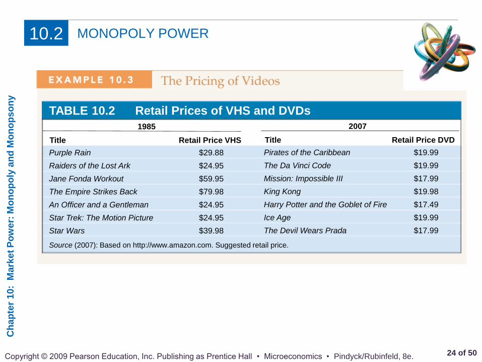
TABLE 10.2 Retail Prices of VHS and DVDs

2007

Title Retail Price DVD

Purple Rain $29.88

Raiders of the Lost Ark $24.95

Jane Fonda Workout $59.95

The Empire Strikes Back $79.98

An Officer and a Gentleman $24.95

Star Trek: The Motion Picture $24.95

Star Wars $39.98

1985

Title Retail Price VHS

Pirates of the Caribbean $19.99

The Da Vinci Code $19.99

Mission: Impossible III $17.99

King Kong $19.98

Harry Potter and the Goblet of Fire $17.49

Ice Age $19.99

The Devil Wears Prada $17.99

Source (2007): Based on http://www.amazon.com. Suggested retail price.

Ch

ap

ter

10

: M

ark

et

Po

we

r: M

on

op

oly

an

d M

on

op

so

ny


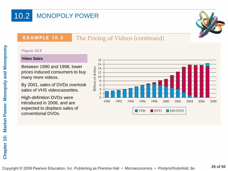
MONOPOLY POWER 10.2

Between 1990 and 1998, lower

prices induced consumers to buy

many more videos.

By 2001, sales of DVDs overtook

sales of VHS videocassettes.

High-definition DVDs were

introduced in 2006, and are

expected to displace sales of

conventional DVDs.

Video Sales

Figure 10.9

Ch

ap

ter

10

: M

ark

et

Po

we

r: M

on

op

oly

an

d M

on

op

so

ny


SOURCES OF MONOPOLY POWER 10.3

If there is only one firm—a pure monopolist—its demand curve is the market

demand curve.

Because the demand for oil is fairly inelastic (at least in the short run), OPEC

could raise oil prices far above marginal production cost during the 1970s and

early 1980s.

Because the demands for such commodities as coffee, cocoa, tin, and copper

are much more elastic, attempts by producers to cartelize these markets and

raise prices have largely failed.

In each case, the elasticity of market demand limits the potential monopoly

power of individual producers.

The Elasticity of Market Demand

Ch

ap

ter

10

: M

ark

et

Po

we

r: M

on

op

oly

an

d M

on

op

so

ny



When only a few firms account for most of the sales in a market, we say that

the market is highly concentrated.

The Number of Firms

● barrier to entry Condition that

impedes entry by new competitors.

Ch

ap

ter

10

: M

ark

et

Po

we

r: M

on

op

oly

an

d M

on

op

so

ny



Firms might compete aggressively, undercutting one another’s prices to

capture more market share.

This could drive prices down to nearly competitive levels.

Firms might even collude (in violation of the antitrust laws), agreeing to limit

output and raise prices.

Because raising prices in concert rather than individually is more likely to be

profitable, collusion can generate substantial monopoly power.

The Interaction Among Firms

Ch

ap

ter

10

: M

ark

et

Po

we

r: M

on

op

oly

an

d M

on

op

so

ny


THE SOCIAL COSTS OF MONOPOLY POWER 10.4

The shaded rectangle and triangles

show changes inc consumer and

producer surplus when moving from

competitive price and quantity, Pc

and Qc,

to a monopolist’s price and quantity,

Pm and Qm.

Because of the higher price,

consumers lose A + B

and producer gains A − C. The

deadweight loss is B + C.

Deadweight Loss from Monopoly Power

Figure 10.10

Ch

ap

ter

10

: M

ark

et

Po

we

r: M

on

op

oly

an

d M

on

op

so

ny



Rent Seeking

● rent seeking Spending money in

socially unproductive efforts to acquire,

maintain, or exercise monopoly.

In 1996, the Archer Daniels Midland Company (ADM) successfully lobbied the

Clinton administration for regulations requiring that the ethanol (ethyl alcohol)

used in motor vehicle fuel be produced from corn.

Why? Because ADM had a near monopoly on corn-based ethanol production,

so the regulation would increase its gains from monopoly power.

Ch

ap

ter

10

: M

ark

et

Po

we

r: M

on

op

oly

an

d M

on

op

so

ny



Price Regulation

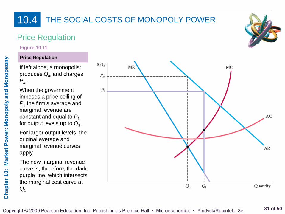
If left alone, a monopolist

produces Qm and charges

Pm.

When the government

imposes a price ceiling of

P1 the firm’s average and

marginal revenue are

constant and equal to P1

for output levels up to Q1.

For larger output levels, the

original average and

marginal revenue curves

apply.

The new marginal revenue

curve is, therefore, the dark

purple line, which intersects

the marginal cost curve at

Q1.

Price Regulation

Figure 10.11

Ch

ap

ter

10

: M

ark

et

Po

we

r: M

on

op

oly

an

d M

on

op

so

ny



Price Regulation

When price is lowered to

Pc, at the point where

marginal cost intersects

average revenue, output

increases to its maximum

Qc. This is the output that

would be produced by a

competitive industry.

Lowering price further, to

P3 reduces output to Q3

and causes a shortage,

Q’3 − Q3.

Price Regulation

Figure 10.11 (continued)

Ch

ap

ter

10

: M

ark

et

Po

we

r: M

on

op

oly

an

d M

on

op

so

ny



Natural Monopoly

A firm is a natural monopoly

because it has economies of

scale (declining average and

marginal costs) over its entire

output range.

If price were regulated to be Pc

the firm would lose money and

go out of business.

Setting the price at Pr yields the

largest possible output consistent

with the firm’s remaining in

business; excess profit is zero.

● natural monopoly Firm that can produce

the entire output of the market at a cost

lower than what it would be if there were

several firms.

Regulating the Price of a Natural

Monopoly

Figure 10.12

Ch

ap

ter

10

: M

ark

et

Po

we

r: M

on

op

oly

an

d M

on

op

so

ny



Regulation in Practice

● rate-of-return regulation Maximum price

allowed by a regulatory agency is based on the

(expected) rate of return that a firm will earn.

The difficulty of agreeing on a set of numbers to be used in rate-of-return

calculations often leads to delays in the regulatory response to changes in

cost and other market conditions.

The net result is regulatory lag—the delays of a year or more usually entailed

in changing regulated prices.

Ch

ap

ter

10

: M

ark

et

Po

we

r: M

on

op

oly

an

d M

on

op

so

ny


MONOPSONY 10.5

● oligopsony Market with only a few buyers.

● monopsony power Buyer’s ability to affect

the price of a good.

● marginal value Additional benefit derived

from purchasing one more unit of a good.

● marginal expenditure Additional cost of

buying one more unit of a good.

● average expenditure Price paid per unit of a

good.

Ch

ap

ter

10

: M

ark

et

Po

we

r: M

on

op

oly

an

d M

on

op

so

ny


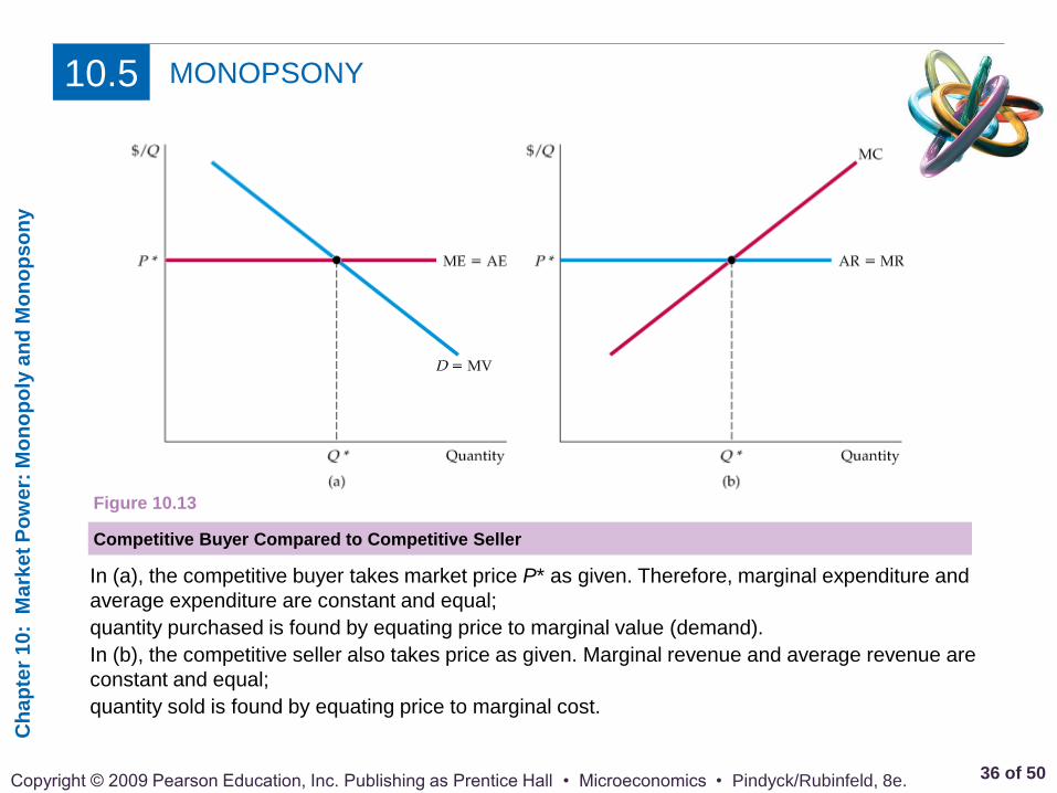
MONOPSONY 10.5

In (a), the competitive buyer takes market price P* as given. Therefore, marginal expenditure and

average expenditure are constant and equal;

quantity purchased is found by equating price to marginal value (demand).

In (b), the competitive seller also takes price as given. Marginal revenue and average revenue are

constant and equal;

quantity sold is found by equating price to marginal cost.

Competitive Buyer Compared to Competitive Seller

Figure 10.13

Ch

ap

ter

10

: M

ark

et

Po

we

r: M

on

op

oly

an

d M

on

op

so

ny


MONOPSONY 10.5

The market supply curve is

monopsonist’s average expenditure

curve AE.

Because average expenditure is

rising, marginal expenditure lies

above it.

The monopsonist purchases quantity

Q*m, where marginal expenditure

and marginal value (demand)

intersect.

The price paid per unit P*m is then

found from the average expenditure

(supply) curve.

In a competitive market, price and

quantity, Pc and Qc, are both higher.

They are found at the point where

average expenditure (supply) and

marginal value (demand) intersect.

Competitive Buyer Compared to

Competitive Seller

Figure 10.14

Ch

ap

ter

10

: M

ark

et

Po

we

r: M

on

op

oly

an

d M

on

op

so

ny


MONOPSONY 10.5

These diagrams show the close analogy between monopoly and monopsony.

(a) The monopolist produces where marginal revenue intersects marginal cost.

Average revenue exceeds marginal revenue, so that price exceeds marginal cost.

(b) The monopsonist purchases up to the point where marginal expenditure intersects marginal value.

Marginal expenditure exceeds average expenditure, so that marginal value exceeds price.

Monopoly and Monopsony

Figure 10.15

Monopsony and Monopoly Compared

Ch

ap

ter

10

: M

ark

et

Po

we

r: M

on

op

oly

an

d M

on

op

so

ny


MONOPSONY POWER 10.6

Monopsony power depends on the elasticity of supply.

When supply is elastic, as in (a), marginal expenditure and average expenditure do not differ by

much, so price is close to what it would be in a competitive market.

The opposite is true when supply is inelastic, as in (b).

Monopsony Power: Elastic versus Inelastic Supply

Figure 10.16

Ch

ap

ter

10

: M

ark

et

Po

we

r: M

on

op

oly

an

d M

on

op

so

ny



Sources of Monopsony Power

Elasticity of Market Supply

If only one buyer is in the market—a pure monopsonist—its monopsony

power is completely determined by the elasticity of market supply. If

supply is highly elastic, monopsony power is small and there is little gain

in being the only buyer.

Number of Buyers

When the number of buyers is very large, no single buyer can have much

influence over price. Thus each buyer faces an extremely elastic supply

curve, so that the market is almost completely competitive.

Interaction Among Buyers

If four buyers in a market compete aggressively, they will bid up the price

close to their marginal value of the product, and will thus have little

monopsony power. On the other hand, if those buyers compete less

aggressively, or even collude, prices will not be bid up very much, and

the buyers’ degree of monopsony power might be nearly as high as if

there were only one buyer.

Ch

ap

ter

10

: M

ark

et

Po

we

r: M

on

op

oly

an

d M

on

op

so

ny



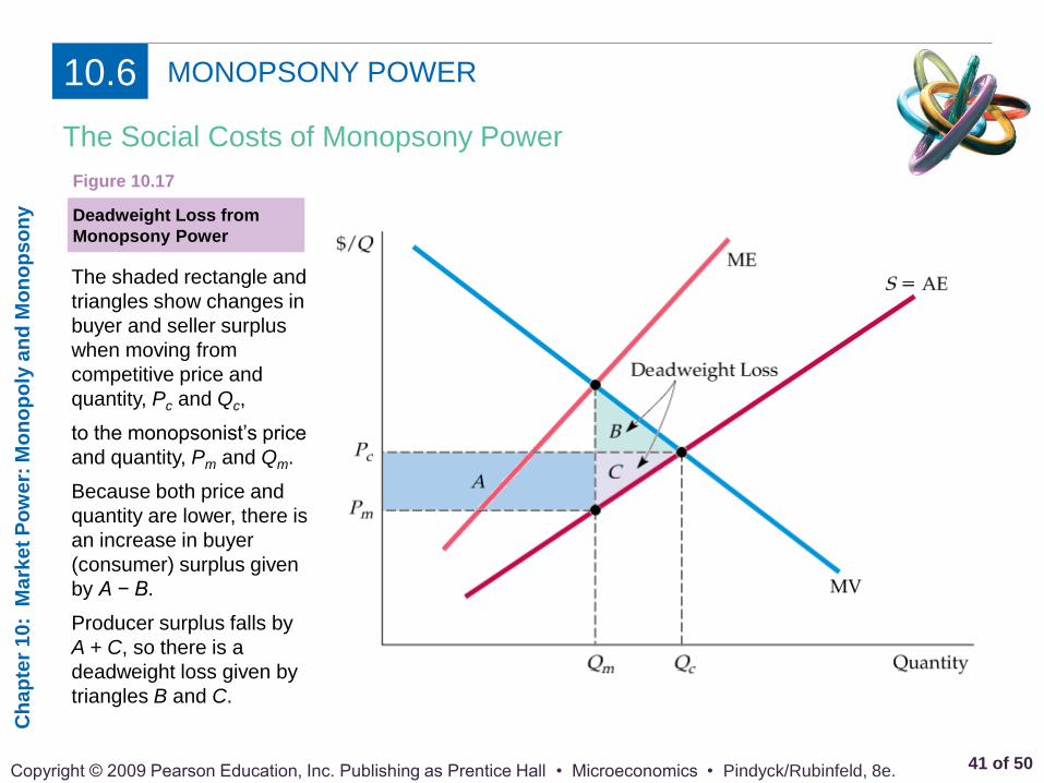
The Social Costs of Monopsony Power

The shaded rectangle and

triangles show changes in

buyer and seller surplus

when moving from

competitive price and

quantity, Pc and Qc,

to the monopsonist’s price

and quantity, Pm and Qm.

Because both price and

quantity are lower, there is

an increase in buyer

(consumer) surplus given

by A − B.

Producer surplus falls by

A + C, so there is a

deadweight loss given by

triangles B and C.

Deadweight Loss from

Monopsony Power

Figure 10.17

Ch

ap

ter

10

: M

ark

et

Po

we

r: M

on

op

oly

an

d M

on

op

so

ny



Bilateral Monopoly

● bilateral monopoly Market with only

one seller and one buyer.

Monopsony power and monopoly power will tend to

counteract each other.

Ch

ap

ter

10

: M

ark

et

Po

we

r: M

on

op

oly

an

d M

on

op

so

ny



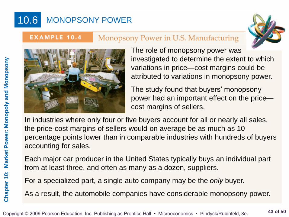
The role of monopsony power was

investigated to determine the extent to which

variations in price—cost margins could be

attributed to variations in monopsony power.

The study found that buyers’ monopsony

power had an important effect on the price—

cost margins of sellers.

In industries where only four or five buyers account for all or nearly all sales,

the price-cost margins of sellers would on average be as much as 10

percentage points lower than in comparable industries with hundreds of buyers

accounting for sales.

Each major car producer in the United States typically buys an individual part

from at least three, and often as many as a dozen, suppliers.

For a specialized part, a single auto company may be the only buyer.

As a result, the automobile companies have considerable monopsony power.

Ch

ap

ter

10

: M

ark

et

Po

we

r: M

on

op

oly

an

d M

on

op

so

ny


LIMITING MARKET POWER: THE ANTITRUST LAWS 10.7

● antitrust laws Rules and regulations

prohibiting actions that restrain, or are

likely to restrain, competition.

There have been numerous instances of illegal combinations. For example:

● In 1996, Archer Daniels Midland Company (ADM) and two other major

producers of lysine (an animal feed additive) pleaded guilty to criminal

charges of price fixing.

● In 1999, four of the world’s largest drug and chemical companies—Roche

A.G. of Switzerland, BASF A.G. of Germany, Rhone-Poulenc of France, and

Takeda Chemical Industries of Japan—were charged by the U.S.

Department of Justice with taking part in a global conspiracy to fix the prices

of vitamins sold in the United States.

● In 2002, the U.S. Department of Justice began an investigation of price

fixing by DRAM (dynamic access random memory) producers. By 2006, five

manufacturers—Hynix, Infineon, Micron Technology, Samsung, and

Elpida—had pled guilty for participating in an international price-fixing

scheme.

Ch

ap

ter

10

: M

ark

et

Po

we

r: M

on

op

oly

an

d M

on

op

so

ny



● parallel conduct Form of implicit

collusion in which one firm consistently

follows actions of another.

● predatory pricing Practice of

pricing to drive current competitors out

of business and to discourage new

entrants in a market so that a firm can

enjoy higher future profits.

Ch

ap

ter

10

: M

ark

et

Po

we

r: M

on

op

oly

an

d M

on

op

so

ny



The antitrust laws are enforced in three ways:

1. Through the Antitrust Division of the Department of Justice.

2. Through the administrative procedures of the Federal Trade Commission.

3. Through private proceedings.

Enforcement of the Antitrust Laws

Antitrust in Europe

The responsibility for the enforcement of antitrust concerns that involve two or

more member states resides in a single entity, the Competition Directorate.

Separate and distinct antitrust authorities within individual member states are

responsible for those issues whose effects are felt within particular countries.

The antitrust laws of the European Union are quite similar to those of the United

States. Nevertheless, there remain a number of differences between antitrust

laws in Europe and the United States.

Merger evaluations typically are conducted more quickly in Europe.

It is easier in practice to prove that a European firm is dominant than it is to show

that a U.S. firm has monopoly power.

Ch

ap

ter

10

: M

ark

et

Po

we

r: M

on

op

oly

an

d M

on

op

so

ny



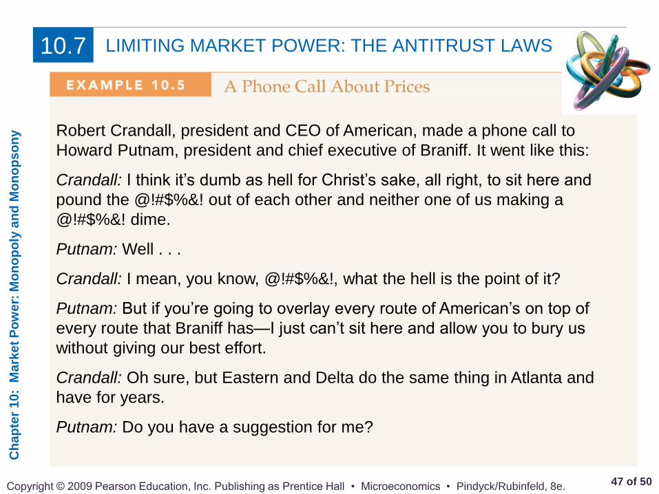
Robert Crandall, president and CEO of American, made a phone call to

Howard Putnam, president and chief executive of Braniff. It went like this:

Crandall: I think it’s dumb as hell for Christ’s sake, all right, to sit here and

pound the @!#$%&! out of each other and neither one of us making a

@!#$%&! dime.

Putnam: Well . . .

Crandall: I mean, you know, @!#$%&!, what the hell is the point of it?

Putnam: But if you’re going to overlay every route of American’s on top of

every route that Braniff has—I just can’t sit here and allow you to bury us

without giving our best effort.

Crandall: Oh sure, but Eastern and Delta do the same thing in Atlanta and

have for years.

Putnam: Do you have a suggestion for me?

Ch

ap

ter

10

: M

ark

et

Po

we

r: M

on

op

oly

an

d M

on

op

so

ny



Crandall: Yes, I have a suggestion for you. Raise your @!#$%&! fares 20

percent. I’ll raise mine the next morning.

Putnam: Robert, we. . .

Crandall: You’ll make more money and I will, too.

Putnam: We can’t talk about pricing!

Crandall: Oh @!#$%&!, Howard. We can talk about any @!#$%&! thing we

want to talk about.

Crandall was wrong. Talking about prices and agreeing to fix them is a clear

violation of Section 1 of the Sherman Act.

However, proposing to fix prices is not enough to violate Section 1 of the

Sherman Act: For the law to be violated, the two parties must agree to

collude.

Therefore, because Putnam had rejected Crandall’s proposal, Section 1 was

not violated.

Ch

ap

ter

10

: M

ark

et

Po

we

r: M

on

op

oly

an

d M

on

op

so

ny



Did Microsoft engage in illegal practices?

The U.S. Government said yes; Microsoft disagreed.

Here are some of the U.S. Department of Justice’s

major claims and Microsoft’s responses.

DOJ claim: Microsoft has a great deal of market power in the market for PC

operating systems—enough to meet the legal definition of monopoly Power.

MS response: Microsoft does not meet the legal test for monopoly power

because it faces significant threats from potential competitors that offer or will

offer platforms to compete with Windows.

DOJ claim: Microsoft viewed Netscape’s Internet browser as a threat to its

monopoly over the PC operating system market. In violation of Section 1 of the

Sherman Act, Microsoft entered into exclusionary agreements with computer

manufacturers and Internet service providers with the objective of raising the

cost to Netscape of making its browser available to consumers.

MS response: The contracts were not unduly restrictive. In any case,

Microsoft unilaterally agreed to stop most of them.

Ch

ap

ter

10

: M

ark

et

Po

we

r: M

on

op

oly

an

d M

on

op

so

ny



DOJ claim: In violation of Section 2 of the Sherman Act, Microsoft engaged in

practices designed to maintain its monopoly in the market for desktop PC

operating systems. It tied its browser to the Windows 98 operating system,

even though doing so was technically unnecessary. This action was predatory

because it made it difficult or impossible for Netscape and other firms to

successfully offer competing products.

MS response: There are benefits to incorporating the browser functionality

into the operating system. Not being allowed to integrate new functionality into

an operating system will discourage innovation. Offering consumers a choice

between separate or integrated browsers would cause confusion in the

marketplace.

DOJ claim: In violation of Section 2 of the Sherman Act, Microsoft attempted

to divide the browser business with Netscape and engaged in similar conduct

with both Apple Computer and Intel.

MS response: Microsoft’s meetings with Netscape, Apple, and Intel were for

valid business reasons. Indeed, it is useful for consumers and firms to agree

on common standards and protocols in developing computer software.

Documents

Market Power: Monopoly and Monopsonynuriyildirim.weebly.com/uploads/5/9/9/7/59978521/ch10.pdfFernando & Yvonn Quijano Prepared by: Market Power: Monopoly and Monopsony E R 10 Copyright