Embed Size (px)
Citation preview

Maritime Performance Evaluation of the Sony XIs Video SystemBrad Stinson, Michael Kuhn and Michael Shannon
Oak Ridge National Laboratory1
1 Bethel Valley Rd, Oak Ridge, TN 37831
ABSTRACTThe Sony XIs imaging system provides a novel method to perform video-based threat detection and assessment over a large area of land or water using a minimal camera-only infrastructure. The XIs employs two camera heads working in unison. One camera head continually scans the scene and builds a super high definition panoramic scene of up to 270º horizontal and 30º vertical field of view (FOV). This panoramic image is composed of up to 180 stitched together high definition (1920x1080 pixel) images. The other camera head is available for live scene viewing or automatic slewing. Difference detection algorithms are implemented which enable threat detection within the panoramic camera’s FOV. Slew to cue functionality of the live camera allows an operator to quickly assess the cause of the detection.
Oak Ridge National Laboratory has completed performance testing of the Sony XIs camera system in day and thermal configurations. The primary goals of these tests are to quantify the optical performance of each system in terms of the probability of assessment (PAS) versus distance for maritime objects. Subjective evaluation of addition system functionality is provided. Finally, the XIs system is compared to other technologies.
INTRODUCTIONThe Sony XIs imaging system shown in Figure 1promises to provide large area coverage with minimal equipment and infrastructure. This is accomplished by using a pan tilt zoom (PTZ) day and/or thermal camera to continuously sweep the horizon and build a large panoramic image from separate high resolution still images. The panoramic camera can cover up to 270º in the horizontal plane and 30º in the vertical. Using separate high definition (HD, 1920x1080 pixel) images from the XIS-5400 daytime camera system, a panoramic image composed of 248,800,000 pixels (248 Mega-pixel) is possible2. Similar functionality is used by the XIS-5310 thermal camera, however the resolution of each image block is 640x480 pixels resulting in a panoramic image composed of up to 36,864,000 pixels (36 Mega-pixel).
Figure 1. XIS-5400 and XIS-5310 Camera Systems
1 Oak Ridge National Laboratory is managed by UT-Battelle, LLC for the U.S. Department of Energy under contract DE-AC05-00OR22725.2 Actual panoramic image resolution is dependent on tile configuration.

The theory of operation is best understood by referring to Figure 2 and Figure 3. The upper image in Figure 2 labeled “Panoramic Image” is the super resolution panoramic image that has been stitched together using one of the two camera heads. In this example, the difference detection algorithm has detected a boat, and the tile where the difference detection is located is enlarged below the panoramic image. Once a difference detection occurs, the second camera (the live camera) is slewed to this tile location in order to show the operator live video footage of that area. This is illustrated in Figure 2 by the “Live Video” label. It is also possible to review before and after images (not videos) from that tile to visualize the image differences that lead to the difference detection. This function is illustrated by the label “Before and After Images.”
Figure 3 is a graphical representation of the panoramic image tiles. Each tile represents a still image captured at 1920x1080 pixels at a preset and fixed focal length3. The blue and green areas represent possible options for limiting the scan area. The scan area is typically limited to only the region of interest, as limiting the size of this area also reduces the time required to complete a full scan.
The primary benefit of the XIs system is replacement of multiple fixed position surveillance cameras with a single two-head unit. Such a system is advantageous for several reasons; reduced cost, reduced maintenance, reduced infrastructure requirements, ease of installation, reduced user fatigue and reduced staff. Assuming equal focal lengths and resolution, the XIs system aims to equal the coverage of up to 180 individual fixed position cameras. However, to successfully replace fixed surveillance camera, the XIs difference detection algorithm must perform reliably. This is because the user is no longer privy to seeing live video from all areas, but must rely on the difference detection algorithms to alert and cue up the area(s) of interest automatically. However, slew to cue operation is generally preferred, as studies have shown that humans are extremely poor detectors when asked to monitor video feeds for more than a few minutes [1]. To date, high security installations have countered the human reliability problem be either integrating detection sensors which alert an operator to refer to video only for assessment purposes or by using video analytics software to analyze the video feed and alert the operator only when movement and/or changes are detected. The XIs system goes one step further into video analytics by expanding the coverage area dramatically. However, in contrast to traditional video analytic based systems, the live video of the entire field of view (FOV) cannot be viewed at once with the XIs system. For this reason, the reliable operation and proper setup of the difference detection system are of critical importance to the success of an XIs system installation.
The remainder of this document will detail how the Sony XIs system was tested, the results of testing the day and thermal cameras and include discussions regarding the difference detection algorithm, enhancement algorithms, additional features and comparisons to other technology.
3 For the camera system tested by ORNL, the panoramic focal lengths are 100mm for the thermal camera and 35.7mm for the day camera. For camera systems with zoom (i.e. the day camera) this focal length is configurable.
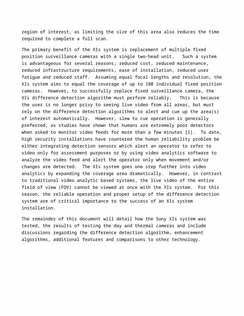
Figure 2. Overview of XIs Operation
Panoramic Image
Live Video
Before and After Images

Figure 3. Panoramic Tiles
TEST SETUP
The Sony XIs camera systems were installed on a sturdy steel structure anchored into concrete. Maximum effort was made to ensure a stable platform in order to minimize movement from wind or other external factors. The camera height was approximately 25 feet above the surface of the water. The cameras were positioned such that they look out onto a bend in the Clinch River near the Oak Ridge National Laboratory (ORNL). This position provided both a wide FOV of approximately 120 degrees and the ability to test with targets at a distance of approximately 2 km. Figure 4 shows the location of the camera and the FOV. Figure 5 shows the cameras installed.
Figure 4. Camera Position and Field of View Diagram

Figure 5. Camera Installation Picture
TEST METHODOLOGY
In testing the Sony XIs camera system, the primary goal was to evaluate the performance with regards to what targets an operator can assess relative to the target distance. To accomplish this goal, video footage was captured under various scenarios with both the day and thermal cameras. These videos were broken into clips which were then used in a survey given to volunteer participants. Participants were asked to evaluate the video clips against one of three assessment levels and inform the test conductor when they were able to assess the target to the specified level. The various clips were used to provide three different boat orientations (broadside, bow and stern) of up to two boat types (pontoon boat and fishing boat). In all cases, the actual Sony XIs Live Viewer software was used to ensure that the video was the same quality/size as what an operator would see.
ORNL defines three assessment levels used in the evaluation of video or still image systems:
Detection is the assessment level where an operator can reliably determine that an object other than normal background is present in the video or image. An example survey question for detection would be, “Given notification that an alarm was tripped, tell me when you can detect that an object other than normal background is present in the video.”
Recognition is the assessment level where the operator can reliably recognize the target type (i.e. boat, swimmer). An example survey question for recognition would be, “The target class is a boat. Given notification that an alarm was tripped, tell me when you can recognize the target class (i.e. boat, jet ski, swimmer, animal, etc.).”
Identification is the assessment level where the operator can reliably identity the class of the target (i.e. fishing boat, pontoon boat, man, woman). An example survey question for identification would be, “The target type is
a fishing boat. Giving notification that an alarm was tripped, tell me when you can identify the target type (i.e. fishing boat, pontoon boat, jet ski, etc.).”
A convenient metric used for evaluation of camera performance is spatial frequency, which is a measure of pixels per meter. This metric is used because it conveniently combines several independent variables, including resolution, target size and horizontal field of view (HFOV) relative to the object distance.
f s=R
HFOV (1)
Where fs is the spatial frequency, R is the system resolution (in horizontal pixels for a digital system) and HFOV is the horizontal field of view (or scene width).
H FOV=W I DFL (2)
Where WI is the imager width in mm, D is the distance to the target and FL is the focal length in mm.
The Sony XIs uses a difference detection algorithm which is triggered based on a user defined minimum pixel count change. The minimum pixel count setting is a critical setting for two reasons: First, nuisance alarms are directly related to the minimum pixel count setting. Setting the value too low will cause small events (e.g. a tree branch blowing in the wind) to be the source of a detection event. Second, the end user will ultimately use the live video feed to assess the situation. Therefore, the end user should decide what level of assessment they desire (detection, recognition or identification) and set the minimum pixel count setting to correspond with the spatial frequency required to achieve that level of assessment. Therefore, the primary objective of the testing the XIs was to evaluate the assessment performance against the three assessment levels. Our hopes are that by determining the spatial frequency required for each level of assessment, it becomes a trivial task to set up the difference detection algorithm to alarm only when it would be possible for the operator to assess the situation at the desired distance and assessment level. In other words, even if the hardware and software is capable of detecting small changes in the scene, if the user is not able to assess what he/she is seeing, the alarm is nothing more than a nuisance. Detection without assessment is not detection [2].
Traditionally, a binomial distribution model is used to derive the probability of assessment versus spatial frequency. Binomial distributions with a high confidence level require that each and every video clip be viewed by each participant. The participant must assign a pass (meaning they can assess the target to the specified level) or fail (they cannot assess the target) to each test. A side effect of this testing method is that many tests are redundant, i.e. they provide little additional data yet require a large amount of time from the participant. For example, if a participant is able to detect a boat at 1000 m, then it follows logically that they will also be able to detect the boat at all distances less than 1000 m. Following this logic, and in an effort to reduce the test time for

each (unpaid) participant to less than 15 minutes, the binomial distribution data was extrapolated for tests where it was highly likely that the participant answers could be predicted. For broadside boat tests, the data is already discrete by approximately 100 m distance due to the boat’s travel path. This data was extrapolated by setting the participant answers to “pass” at all distance shorter than the distance they were first able to accurately assess the target. For stern and bow orientation tests, the data was made discrete by breaking the boat path into 20 m bins. The data was then extrapolated by setting participant answers to “pass” at all distances shorter than the distance they were able to first correctly assess the target.
The binomial distribution model results allow us to calculate the probability of assessment (PAS) at a high confidence level versus spatial frequency. A theoretical model called the Johnson Criteria Model (Equations 3 and 4) is then used to extend the empirically determined results to any distance based on the spatial frequency which provides a 50% PAS. Using the Johnson model it is possible to estimate the PAS for each assessment level and each target type at any distance [3]. This capability not only allows the end user to visualize the PAS across a wide range of distances for each scenario (target type, assessment level, target orientation) but also allows them to set up the XIs detection algorithm by selecting the desired PAS, then determining the pixel change setting that will trigger the XIs detection algorithm only when assessment can take place.
P ( N )=( N
N 50)E
1+( NN50 )
E (3)
Where
E=2.7+0.7 ∙( NN50 ) (4)
P(N) is the target Johnson model transfer probability function, N is the spatial frequency (which can be put in terms of distance) and N50 is the spatial frequency required by an observer to correctly assess the target with a probability of 50%. The Johnson model assumes that N will be in terms on line pairs, however for the case of digital systems, N can be found by f s /2.
DAY CAMERA PERFORMANCE
The XIS-31HCX day camera uses a ½” 3 CCD image 1.5 million pixel 7 mm imager. The output signal is 1920x1080 pixels, but when viewed in the Live Viewer software, the image is cropped to 1024x768. The full resolution image is available via an SD-HDI interface. The day camera includes a zoom lens which ranges from 6.7 to 241mm (66mm – 1244mm 35mm equivalent). Aperture values are F3 (wide) and F3.9 (tele). It operates to 0.014 lux. For all assessment tests, supplemental image processing algorithms were turned off. Gain and iris

settings were adjustment manually by the test conductors to provide the best subjective image quality. Focus was set to automatic.
The day test was conducted with a 16 foot fishing boat with an outboard motor and 2 passengers. The tests occurred on December 1, 2011 and began at 12:30. Weather conditions were clear skies, calm winds and no precipitation. The temperature was 45º F with a humidity of 76%.
The test goals where to capture video footage of the boat with variable orientation and at variable distances from the camera. This was accomplished by making multiple broadside passes approximately orthogonal to the midpoint of the camera’s horizontal FOV. Each broadside pass was approximately 100 meters further or closer to the camera than the previous pass. Bow and stern orientations were accomplished by having the boat follow a path parallel and in close alignment with the midpoint of the camera’s FOV. GPS data from the test is shown in Figure 11. The boat maintained an average speed of approximately 13 knots throughout all tests.
In order to evaluate the camera performance, a survey was conducted as discussed in the Test Methodology section above. Broadside video footage from these tests were broken into short clips approximately 10 seconds long. Stern and bow alignment video footage was separated into clips covering the time span required for the boat to travel from the furthest point (~2 km) to the closest point (20 m). Each of these clips was repeated for the two boat types and each clip was evaluated for the three different assessment levels. The result was eight different survey questions. Test subjects were volunteers from within the ORNL workforce.
Survey results for each question are summarized below in Table 0-1. For each survey question, a distance is noted based on the participant’s answer. This distance is converted into spatial frequency (pixels/m) based on the specifications of the camera system (imager size, focal length and horizontal FOV). A histogram of the survey answer distribution is provided in the Appendix..

Figure 6. GPS Data for Day Test
The mean and standard deviation (σ) is provided for each survey question. A calculation of maximum assessment distance was used in lieu of empirical data because it was not possible to test maximum range at this location due to physical limitations and obstructions. These numbers are therefore only theoretical extrapolations, based on the mean spatial frequency observed at the widest focal range and the maximum focal length of 241mm4. The maximum assessment distance shown in Table 0-1 is a theoretical value calculated from equation 5, where D is the calculated distance, R is the resolution, WI is the imager width, FL is the focal length at full zoom (241mm) and fs is the empirically derived mean spatial frequency from the survey results.
D= RW I
FLf s
(5)
It should be noted that the maximum assessment distance is almost certainly overestimated for many of the cases in Table 0-1. The reasons for this are that the curvature of the earth limits visibility of targets to approximately 20 km assuming the camera is 30 m higher than the target and only 5 km if the target is at the same height. Other
4 The XIS-31HC model has a maximum focal length of 127mm at F1.9
effects limit visibility at extreme distances including atmospheric diffraction, shimmering and poor image stabilization.
The focal length of the day camera was fixed at the widest angle (12.8 mm indicated) for these test. This was done to maximize the horizontal field of view and create a scenario that would make it most difficult for participants to assess the boat at a distance. As mentioned, the test area imposes a natural limit of about 2 km maximum distance from the camera. The survey results for broadside boat detection are questionable because all participants where able to perform a detection assessment even at maximum distance. It is apparent from the histogram data in the Appendix that 2 km is not sufficient to achieve statistically valid data for the broadside boat tests at the detection assessment level. Unfortunately, this flaw in the data does not have an easy fix, as 2 km is the maximum distance possible in the test area.
The survey data shows a general trend of standard deviation increasing proportional to the assessment level. That is, when participants were asked to indentify targets there was a wider variety in the distance participants were able to reliably assess the targets. The opposite trend was true as well, when participants were asked only to detect the presence of a target the answers were more consistent.
Table 0-1. Day Camera Survey Results
Test Description MSF (pixels/m) Standard Deviation Max Assessment Distance (based on MSF)
Fishing BoatBroadsideAssessment Level = Detection
1.85 0.0 36.7km6
Fishing BoatBroadsideAssessment Level = Recognition
2.6 0.7 25.3km6
Fishing BoatBroadsideAssessment Level = Identification
3.9 1.4 16.9km6
Fishing BoatBow AlignmentAssessment Level = Detection
2.7 0.5 24.5km6
Fishing BoatBow AlignmentAssessment Level = Recognition
4.6 3.0 14.2km6
Fishing BoatBow AlignmentAssessment Level = Identification
10.5 8.9 6.3km
Fishing BoatStern AlignmentAssessment Level = Identification
10.9 3.5 6.0km
Fishing BoatStern AlignmentAssessment Level = Recognition
5.9 2.1 11.2km6
5 All survey participants were able to detect the boat at the maximum distance. This value is therefore an error on the 6 Real maximum assessment distance is likely less than these values due to image degradation effects at extreme distances and/or earth curvature limits.

The Johnson Criteria model was used to approximate the PAS versus all distances. In order to calculate the Johnon model, the data was first extrapolated into a binomial model (see Test Methodology section). Example data from this extrapolation is shown in Figure 7 for the fishing boat in broadside orientation and recognition assessment. The Matlab code used to perform this extrapolation is provided in the Appendix. From this data, the Johnson model can be derived using the N50 value, which is the spatial frequency which provides 50% PAS (1 pixel/m in this example).
Figure 7. Day Camera, Broadside Recognition Binomial Data Extrapolation
The Johnson Criteria model for this test is shown in the Figure 8 below. In order to confirm the validity of the model, the Johnson criteria is plotted against the extrapolated binomial data set based on the survey results. The extrapolated binomial test data is plotted with the upper (blue) and lower (red) bounds shown for a 95% confidence level.7
7 Confidence intervals were calculated using the Adjusted Wald method [4].

Figure 8. Johnson Model, Day Camera, Broadside Orientation, Recognition Assessment
Johnson models are shown below for the common scenarios of bow orientation with a recognition assessment level (Figure 9) and stern orientation with an identification assessment level (Figure 10). All Johnson models presented assume that maximum focal length is used for assessment. Binomial data extrapolation plots and Johnson models for all tests can be found in the Appendix.
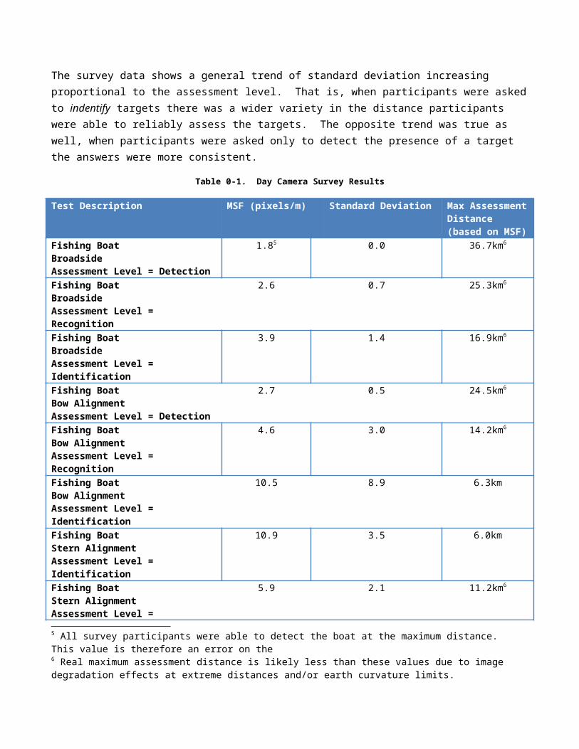
Figure 9. Johnson Model, Bow Orientation, Recognition Assessment
Figure 10. Johnson Model, Stern Orientation, Identification Assessment

THERMAL CAMERA PERFORMANCE
The thermal camera uses a 0.3 million pixel (640x480) 15 mm sensor with a fixed focal length lens of 100 mm and fixed aperture of F1.4. The thermal imager is sensitive from 8 to 14 um wavelengths. For all tests, supplemental image processing algorithms were turned off. Gain and iris settings were adjustment manually by the test conductors to provide the best subjective image quality. Focus was set to automatic.
Two separate nights were used to capture video footage. Night one used a 16 foot fishing boat with an outboard motor and 2 passengers. The first test occurred on May 10, 2011 and began at 21:00. Sunset for this day was at 20:30. Weather conditions were partly cloudy skies, calm winds, no precipitation and a ambient temperature of 80ºF with a humidity of 78%. The moon phase was 52% with the moonrise occurring at 16:59 and moonset at 8:03 the following day. Night two used a 22 foot pontoon boat with an outboard motor and two passengers. This test occurred on May 19, 2011 and began at 21:09. Sunset for this day was 20:39. Weather conditions were clear skies, calm winds, no precipitation with an ambient temperature of 64ºF and humidity of 69%. The moon phase was 92% but the moonrise didn’t occur until 23:15, therefore this test was conducted with no moon light.
The test goals where to capture video footage of the two boat types with variable orientation and variable distance from the camera. This was accomplished by making multiple broadside passes approximately orthogonal to the midpoint of the camera’s horizontal FOV. Each broadside pass was approximately 100 meters further or closer to the camera than the previous pass. Bow and stern orientations were accomplished by having the boat follow a path parallel and in close alignment with the midpoint of the camera’s FOV. GPS data from the first night test is shown in Figure 11. The boat maintained an average speed of approximately 13 knots throughout all tests.
In order to evaluate the thermal camera performance, a survey was conducted as discussed in the Test Methodology section above. Broadside video footage from these tests was broken into short clips approximately 10 seconds long. Stern and bow alignment video footage was separated into clips covering the time span required for the boat to travel from the furthest point (~2 km) to the closest point (20 m). Each of these clips was repeated for the two boat types and each clip was evaluated for the three different assessment levels. The result was 16 different survey questions. Future more, the two boat passengers were asked to stand up in the boat with bow alignment and the boat travelling directly toward the camera position. This clip was used as an evaluation of personnel recognition and identification assessment performance, bringing the total survey question count to 18. As before, test subjects were volunteers from within the ORNL workforce.

Figure 11. GPS Data for Night Test 1
Survey results for each question and summarized below in Table 0-2. For each survey question, a distance is calculated based on the participant’s answer. This distance is converted to spatial frequency (pixels/m) based on the camera specifications (imager size, focal length and horizontal field of view). The mean and standard deviation (σ) is provided for each survey question. Histograms of the survey data can be found in the Appendix. Unlike the day camera, the thermal camera has a fixed lens of 100 mm. Therefore, there is no need for zoom lens compensation and the maximum assessment distance shown in Table 0-2 is based on empirical data.
The survey results follow expected patterns, i.e. the larger pontoon boat was detected at a further distance than a smaller fishing boat (2.3 pixels/m mean versus 2.6 pixels/m mean) . It is apparent that standard deviation of the results increases with assessment level. In other words, when asked when they could identify the target class, the participant’s answers were more widely distributed, with the worst case being personnel identification, which had a mean spatial frequency of 72 pixels/m with a standard deviation of 37.2.
Table 0-2. Thermal Camera Survey Results
Test Description MSF (pixels/m) Standard Deviation Max Assessment Distance
Fishing BoatBroadsideAssessment Level = Detection
2.6 0.4 1.6 km
Fishing BoatBroadside
3.4 0.4 1.2 km

Assessment Level = RecognitionFishing BoatBroadsideAssessment Level = Identification
7.0 1.8 608 m
Pontoon BoatBroadsideAssessment Level = Detection
2.3 0.3 1.9 km
Pontoon BoatBroadsideAssessment Level = Recognition
3.1 0.5 1.4 km
Pontoon BoatBroadsideAssessment Level = Identification
6.3 1.8 682 m
Fishing BoatBow AlignmentAssessment Level = Detection
3.5 0.1 1.2 km
Fishing BoatBow AlignmentAssessment Level = Recognition
4.5 1.7 941 m
Fishing BoatBow AlignmentAssessment Level = Identification
7.5 3.0 570 m
Fishing BoatStern AlignmentAssessment Level = Recognition
6.0 1.4 713 m
Fishing BoatStern AlignmentAssessment Level = Identification
4.9 1.1 866 m
Pontoon BoatStern AlignmentAssessment Level = Recognition
6.3 1.7 682 m
Pontoon BoatStern AlignmentAssessment Level = Identification
5.3 1.4 806 m
Pontoon BoatBow AlignmentAssessment Level = Detection
2.3 0.2 1.9 km
Pontoon BoatBow AlignmentAssessment Level = Recognition
2.9 0.6 1.5 km
Pontoon BoatBow AlignmentAssessment Level = Identification
4.9 1.1 866 km
PersonnelFrontal StandingAssessment Level = Recognition
10.0 1.5 427 m
PersonnelFrontal StandingAssessment Level = Identification
72.0 37.2 59 m

The survey data was extrapolated into a binomial model as explain in the Test Methodology section. An example results of this extrapolation is shown in Figure 12 for a fishing boat in the broadside orientation at a recognition assessment level.
Figure 12. Thermal Camera, Fishing Boat, Broadside Recognition Binomial Data Extrapolation
As previously mentioned, from the binomial model, the N50 value can be determined for each test as the spatial frequency / 2 when the probability of assessment is 50%. In Figure 12, this is approximately 3.8 pixels/m. The Johnson model then provides a prediction of the PAS for any given distance. Figure 13 and Figure 14 illustrate the Johnson model results for 2 example data sets. Johnson models for all tested cases are available in the Appendix.

Figure 13. Johnson Model, Thermal Camera, Broadside Fishing Boat, Recognition Assessment
Figure 14. Johnson Model, Thermal Camera, Bow Alignment, Identification Assessment

PANORAMIC DIFFERENCE DETECTION
As mentioned in the introduction, the primary benefit of the XIs system is the ability to replace multiple fixed position security cameras with only two. To successfully achieve this requires that the panoramic image difference detection system operate such that nuisance alarms are minimized while actual threats are detected as soon as possible.
Setup of the difference detection algorithm consists of three parts: setting the approximate pixel count, masking off areas of non-interest or likely false alarms and using the built-in algorithms to reject pixel changes from naturally occurring motion (i.e. waves).
Pixel Count Settings
Based on the tests from the previous section, the appropriate pixel count size can be selected based on the desired assessment performance. The end user should first define the following variables: Target type and size, desired PAS and desired assessment level. With these variables defined, the end user can refer to the Johnson models in the Appendix for the craft closest in type/size at the desired assessment level. For example, if the end user wishes to target a 16 foot ski boat, and they wish to be alerted when they have a 80% PAS of identifying the target as a ski boat, they can refer to the Johnson Model in the Appendix (Day Camera, Fishing Boat, Bow Alignment, Identification Assessment). From this model, PAS of 80% occurs at a distance of 6 km. The Johnson models are based on maximum zoom distance (for the day camera) but because the camera used for panoramic image difference detection is not maximally zoomed, the spatial frequency must be calculated using the panoramic focal length (35.7 mm for the ORNL installation). Solving equation 5 for fs at a distance (D) of 6 km, resolution of 1920 pixels and a focal length (FL) of 35.7:
f s=1920
6,000 ∙ 735.7
=1.6 pixels /m(6)
We now need to estimate the target width (WT) of the boat relative to the camera. Since we used bow alignment (the worst case option), WT is the boat width relative to the camera in that orientation, which is estimated at 2 meters. Therefore, the total number of pixels (px) required for the panoramic difference detection is:
px=f s ∙W T=19.5 ∙2=3.3 pixels (7)
This process can also be used to optimize the focal length of the panoramic camera. If for the desired assessment scenario, the resultant pixel count too low (i.e. less than 1) then the zoom setting of the panoramic camera can be increased until the pixel count reaches a reasonable level. Of course, as panoramic zoom is increased, the tile count must be increased to provide equivalent coverage.
Note that in practice, setting a low pixel count for the detection threshold algorithm and/or zooming in the panoramic camera will increase the nuisance alarm rate. Therefore, the desired assessment scenario will have to be balanced with the nuisance alarm rate requirements.

Masking
Masking is simply denoting areas of non-interest to prevent those areas from contributing to the nuisance alarm rate. For the test area at ORNL, it made sense to mask out the areas above the shore line to eliminate cloud movement, tree movement, birds, etc., since we were only concerned with maritime targets. Masking will vary by installation. The XIs system provides an easy to use masking tool that allows the user to “paint” areas that should be masked. One important note is that the user should be aware when masking distant shorelines that distant targets can be unexpectedly masked out during this process because the target is back dropped by the shoreline at extreme distances. This problem can be reduced by mounting the camera as high as possible.
Filtering
The XIs software includes filters to reduce the nuisance alarms caused by wave activity. The underlying settings for this filter are unknown, but can most likely be modified to work best with specific environments. The Clinch River test area is normally quite calm. The wave activity filter worked reasonable well, notably reducing the nuisance alarm rate when it was used, but nuisance alarms were still generated about 1/minute due to water movement. It is expected that the algorithm settings could be refined to improve this, but it is not something that ORNL was trained on, so the settings were not modified.
Scan Time
Scan time refers to the total time required to build one super resolution panoramic image. Scan time is important to the detection algorithm because if it takes too long to build the panoramic image, a target could have made significant progress into the protected area before detection. Although improbable, a long scan time could make it possible for an object to enter and leave the detection zone undetected. Scan time is dependent on the tile count, which can vary based on the tile configuration. Example configurations for the day camera are shown in Figure 15. In the case of the test at ORNL, the tiles provide a 157º horizontal field of view and a 25º vertical field of view (56 tiles, 14x4 configuration). The scan time takes 28.8 seconds. For an object to penetrate undetected it would have to be able to move through vertical tiles ahead of the scan line, which moves from top left, left to right and then right to left as it moves down the tiles. In the ORNL configuration that would require the object to travel about 0.6 kilometers in 14.4 seconds, or 150 kmph (93.2 mph). Of course at these speeds, significant wakes would be created which would likely be detected even if that craft itself was not.

Figure 15. Tile Options and Corresponding Scan Times

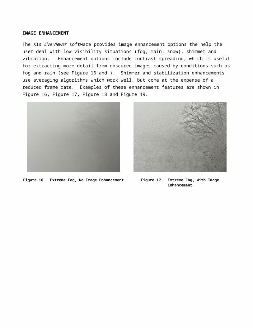
IMAGE ENHANCEMENT
The XIs Live Viewer software provides image enhancement options the help the user deal with low visibility situations (fog, rain, snow), shimmer and vibration. Enhancement options include contrast spreading, which is useful for extracting more detail from obscured images caused by conditions such as fog and rain (see Figure 16 and ). Shimmer and stabilization enhancements use averaging algorithms which work well, but come at the expense of a reduced frame rate. Examples of these enhancement features are shown in Figure 16, Figure 17, Figure 18 and Figure 19.
Figure 16. Extreme Fog, No Image Enhancement Figure 17. Extreme Fog, With Image Enhancement
Figure 18. Heavy Rain, Enhancement on Left, No Enhancement on Right
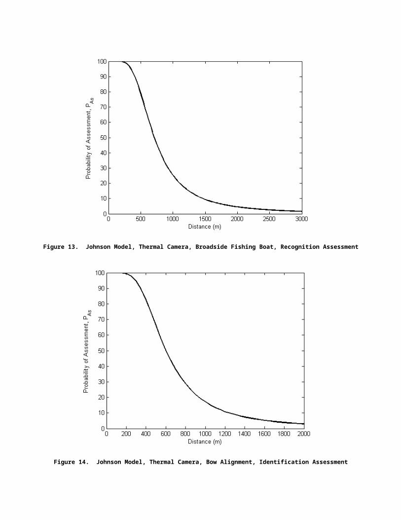
Figure 19. Snow and High Winds, Enhancement on Left, No Enhancement on Right8
SOFTWARE FEATURES
The Live Viewer features a digital resolution boost (DRB) option which is useful for scenarios where the user wishes to digitally zoom in on an object or region of interest. The user can position the mouse on the desired location and a box is opened with a digitally zoomed portion of the frame. This feature is useful for quick views of markings (license plates or boat marking) without using an optical zoom which requires time and the user to lose some situational awareness. An example of DRB is shown in Figure 20.
The Live Viewer software implements a tracking function, in which the pan, tilt and zoom controls are automatically adjusted to keep the camera centered on a selected target. An example of the tracking function is shown in Figure 21.
The Live Viewer software estimates the coordinates (latitude and longitude) of the center of the FOV. Cross hairs and coordinate values are displayed on the video feed. The accuracy of this system was not tested, but it is a promising addition considering the XIs aims to be both a detection and assessment system. Being able to estimate the location of detected targets and send this data to other situational awareness systems is critical. The coordinate function is shown in Figure 22.
8 In the right side of the image, there was substantial movement at the XIs due to extreme winds and being fully zoomed. The stabilization enhancement was able to compensate for these condition.

Figure 20. XIs Live Viewer Digital Resolution Boost Function
Figure 21. XIs Live Viewer Tracking Function

Figure 22. XIs Live Viewer Coordinates Function
GENERAL OBSERVATIONS
The Live Viewer software provided with the XIs crops the image to 1024x768 pixels. We believe that this is an image crop, not a decimation-based resize, so there is no loss in resolvable details, only a loss in the outside portion of the image frame. It is unclear why this crop is implemented, but we suspect it is to improve performance of the image enhancement algorithms (a 1024x768 frame contains only 38% of the pixels of a full 1920x1080 frame). We would prefer the option to see the full resolution HD image if hardware is available to support it. Sony does provide an HD SDI interface, however this is limited to approximately 285 ft which make its use prohibitive in some environments [5]. Additionally, using the direct connection bypasses the software enhancement features available in the Live Viewer software. There also appears to be some compression artifacts when viewing the video in the Live Viewer software. Again, it is unclear why the video is compressed. We assume this is due to network bandwidth limitations, but our own network analytics shown that a Gigabit network has ample overhead available for increased data rates. We would prefer to minimize or even eliminate compression if the network bandwidth is available.
The typical system installation consists of two controlling computers, one of which handles the panoramic image and one of which handles the live view. Strangely, the two software applications have been developed on different operating system platforms. The panoramic software runs in the Linux environment while the live view software runs on Windows. The two applications remain interoperable, i.e. the panoramic software can cause the live view software to slew to the target location. Two different operating systems was not an issue in practice,

but in today’s cyber security environment, we question the need to keep two operating systems updated and patched with without a clear need to do so.
TECHNOLOGY COMPARISON
In comparison to standard surveillance cameras, the primary benefit of the XIs system a dramatic reduction in the number of cameras required to cover an equivalent space. However, the XIs system does pose some limitations when compared to a surveillance camera array. For example, pre-event buffering is not possible because unlike fixed surveillance cameras, the cameras are not on target at all times. For security applications dependent on pre-event buffering for analysis of the event, the XIs is not appropriate. There is also intrinsic delay between when the target enters the area and when the panoramic camera system detects the target. The size of this delay varies based on the number of tiles and the location of the target relative to the panoramic scan sequence. In a worst case scenario, it could be approximately 60-70 seconds between when a target enters the monitored area and when the XIs system detects it. However, human monitored surveillance cameras have been shown to be quite ineffective, so in practice we would expect the XIs to provide a distinct advantage over fixed arrays despite the time delay [1].
In comparison to ground surveillance radar (GSR), the XIs offers similar detection capabilities relative to published target size and distance capabilities. ORNL does not have GSR data for the test area, so direct performance comparisons could not be made. The XIs system requires line of sight for detection (and obviously for assessment), while GSR system can be used in fog, snow and light precipitation without hindrance [6].
GSR systems are designed to not only detect targets but also to provide accurate location and travel vectors of those targets. This is an area where GSR systems currently surpass the XIs. While the XIs does have a coordinate overlay feature, there is currently no information regarding location or travel vector of each detected threat. As a stand alone system, the exclusion of this feature is acceptable, but if the XIs was to feed a situational awareness system as both a detection device and an assessment device it would need the capability to estimate target location and target travel vector if it is to compete with GSR systems.
GSR systems are active in the sense that electromagnetic waves are sent out into the environment, where they are reflected back towards to source. Should a facility have limitations on the use of active radar systems, the XIs system presents a viable alternative to GSR.
It is expected that the XIs system will offer an improved assessment rate (successful assessments per detection) relative to sensor and camera hybrid systems. For a hybrid sensor and camera system, the cause of the sensor trip is often unable to be determined by video review. For example, a small leaf could trigger an infrared beam sensor, but be too small to be seen on a video system. Generally these situations require human deployment to the area since the cause of the alarm could not be assessed with video. With a video analytics system, it is assured that there was an actual change in the scene and therefore successful assessment rates are expected to be higher.
The XIs has the benefit of tight integration with other camera systems. Should an end-user have an extensive video monitoring solution in place, the XIs may be added to that system such that it extends video coverage seamlessly and leverages existing surveillance cameras to bolster its own capabilities.

CONCLUSION
The tests conducted detail the performance characteristics of the XIs system in a maritime environment. The Johnson models provide predictions of probability of assessment versus distance. It has been shown how this data can be used by the end user to define the detection system’s pixel count size based on the target object, desired assessment level and assessment probability.
The XIs system is a unique and well-executed video system providing detection and assessment options previously unavailable in a purely optical system. The primary benefits include a single well-integrated system providing both assessment and detection over a large region. It is our opinion that the two most promising applications of this technology are high-traffic maritime environments and high-traffic land applications with sparse vegetation. The panoramic image and pixel change detection algorithms area ideal for high traffic environments where the operator needs to assess potential threats on a frequenct basis. In these environments, the XIs provides a powerful situational awareness advantage by remaining in the visual space, allowing the operator to stay aware of both the big picture and individual targets.
REFERENCES
[1] N. Sulman, T. Sanocki, D. Goldgof, R. Kasturi, “How Effective is Human Video Surveillance Performance”, 19th International Conference on Pattern Recognition, 2008, pgs 1-3.
[2] M. Garcia, “The Design and Evaluation of Physical Protection Systems, 2nd Edition” Butterworth-Heinemann, 2008.
[3] J. Johnson, “Analysis of Image Forming Systems,” Image Intensifier Symposium, AD 220160 (Warfare Electrical Engineering Department, U.S. Army Research and Development Laboratories, Ft. Belvoir, VA., 1958, pp. 244-273
[4] A. Agresti and BA Coull, “Approximate is better than “Exact” for Interval Estimation of Binomial Proportions.” The American Statistician. 52:119-126, 1998.
[5] Extron Electronics, Distribution High Definition, url: http://www.extron.com/company/article.aspx?id=lvdg_ts, accessed December 20, 2011.
[6] L. Varshney, “Ground Surveillance Radars and Military Intelligence,” Technical Report, Syracuse Research Corporation, December 30, 2002.

APPENDIX
Day Camera Survey Histograms
1.80
5
10
15
20
25
30
35
Spatial Frequency (pixel/meter)
Freq
uenc
y
Fishing Boat, BroadsideAssessment Level = Detection
Mean = 1.8, σ = 0.0
1.8 2.2 3 3.8 4.40
2
4
6
8
10
12
14
Spatial Frequency (pixel/meter)
Frequ
ency
Fishing Boat, BroadsideAssessment Level = Recognition
Mean = 2.6, σ = 0.7
3 3.4 3.8 4.4 4.8 5.1 6.6 80
2
4
6
8
10
12
14
16
18
20
Spatial Frequency (pixel/meter)
Frequ
ency
Fishing Boat, BroadsideAssessment Level = Identification
Mean = 3.9, σ = 1.4
2.4 2.5 2.6 2.7 2.8 3 5.40
1
2
3
4
5
6
7
8
9
10
Spatial Frequency (pixel/meter)
Frequ
ency
Fishing Boat, Bow AlignmentAssessment Level = Detection
Mean = 2.7, σ = 0.5
2.6 2.8 2.9 3 3.1 3.2 3.3 3.4 3.5 3.6 3.8 3.9 5.2 7.2 8 9.1 12.3 12.50
1
2
3
4
5
6
Spatial Frequency (pixel/meter)
Frequ
ency
Fishing Boat, Bow AlignmentAssessment Level = Recognition
Mean = 4.6, σ = 3.0
3.8 4.2 4.5 4.9 5.6 5.9 8 8.5 9.2 9.7 12 14.5
18.4
32.4
0
0.5
1
1.5
2
2.5
Spatial Frequency (pixel/meter)
Freq
uenc
y
Fishing Boat, Bow AlignmentAssessment Level = Identification
Mean = 10.5, σ = 8.9
4 4.7 6 6.3 7 8.5 8.7 9.1 9.4 9.6 9.9 10.310.710.911.411.612.413.313.613.914.314.715.516.4
0
0.5
1
1.5
2
2.5
3
3.5
Spatial Frequency (pixel/meter)
Frequ
ency
Fishing Boat, Stern AlignmentAssessment Level = Identification
Mean = 10.9, σ = 3.2
3 3.1 3.4 3.7 3.9 4.1 4.2 4.4 4.5 4.6 5 5.1 5.3 5.5 5.7 6.2 6.3 6.5 6.9 7.2 7.3 7.5 7.6 7.8 9.1 10.7
0
0.5
1
1.5
2
2.5
3
3.5
Spatial Frequency (pixel/meter)
Frequ
ency
Fishing Boat, Stern AlignmentAssessment Level = Recognition
Mean = 5.9, σ = 2.1

Thermal Survey Histograms
2.2 2.7 3.1 3.60
2
4
6
8
10
12
Spatial Frequency (pixels/m)
Freq
uenc
y
Fishing Boat, BroadsideAssessment Level = Detection
Mean = 2.6, σ = 0.4
2.7 3.1 3.6 3.80
2
4
6
8
10
12
14
16
Spatial Frequency (pixels/m)
Freq
uenc
y
Fishing Boat, BroadsideAssessment Level = Recognition
Mean = 3.4, σ = 0.35
3.6 6.2 7.5 9.4 11.20
2
4
6
8
10
12
14
16
18
Spatial Frequency (pixels/m)
Freq
uenc
y
Fishing Boat, BroadsideAssessment Level = Identification
Mean = 7.0, σ = 1.8
2.1 2.5 2.6 2.80
2
4
6
8
10
12
14
16
Spatial Frequency (pixels/m)
Frequ
ency
Pontoon Boat, BroadsideAssessment Level = Detection
Mean = 2.3, σ = 0.3
2.5 2.6 2.8 3 3.5 4.10
1
2
3
4
5
6
7
8
9
Spatial Frequency (pixels/m)
Freq
uenc
y
Pontoon Boat, BroadsideAssessment Level = Recognition
Mean = 3.1, σ = 0.5
4.5 5 5.2 6.3 7.3 9.30
1
2
3
4
5
6
7
8
9
10
Spatial Frequency (pixels/m)
Frequ
ency
Pontoon Boat, BroadsideAssessment Level = Identification
Mean = 6.3, σ = 1.8

3.4 3.5 3.6 3.7 3.80
2
4
6
8
10
12
Spatial Frequency (pixels/m)
Freq
uenc
y
Fishing Boat, Bow AlignmentAssessment Level = Detection
Mean = 3.5, σ = 0.1
3.5 3.6 3.7 3.8 3.9 4.1 4.2 5.1 5.3 8 8.2 9.30
1
2
3
4
5
6
Bin Range
Freq
uenc
y
Fishing Boat, Bow AlignmentAssessment Level = Recognition
Mean = 4.5, σ = 1.7
5.1 5.3 5.5 5.6 5.8 6.2 6.7 7.3 7.6 10.3 10.6 12.4 12.9 14.90
0.5
1
1.5
2
2.5
3
3.5
Spatial Frequency (pixels/m)
Freq
uenc
y
Fishing Boat, Bow AlignmentAssessment Level = Identification
Mean = 7.5 ,σ = 3.0
3.9 4.4 4.6 5 5.1 5.2 5.4 5.8 6 6.2 6.4 6.5 6.6 6.9 8.9 9.70
0.5
1
1.5
2
2.5
Spatial Frequency (pixels/m)
Freq
uenc
y
Fishing Boat, Stern AlignmentAssessment Level = Recognition
Mean = 6.0, σ = 1.4
3.9 4 4.1 4.5 4.6 5.4 6.2 6.70
0.2
0.4
0.6
0.8
1
1.2
Spatial Frequency (pixels/m)
Freq
uenc
y
Fishing Boat, Stern AlignmentAssessment Level = Identification
Mean = 4.9, σ = 1.1
3.7 4.5 4.6 4.7 4.8 4.9 5 5.1 6.9 7 7.2 7.3 7.4 9 9.3 9.50
0.5
1
1.5
2
2.5
Spatial Frequency (pixels/m)
Freq
uenc
y
Pontoon Boat, Stern AlignmentAssessment Level = Recognition
Mean = 6.3 ,σ = 1.7

3.7 3.8 4.1 4.2 4.3 4.4 4.5 4.6 4.7 4.8 4.9 5 6.9 7 7.1 7.4 7.8 7.90
0.5
1
1.5
2
2.5
Spatial Frequency (pixels/m)
Freq
uenc
y
Pontoon Boat, Stern AlignmentAssessment Level = Identification
Mean = 5.3, σ = 1.4
2.1 2.2 2.5 2.6 2.70
2
4
6
8
10
12
Spatial Frequency (pixels/m)
Frequ
ency
Pontoon Boat, Bow AlignmentAssessment Level = Detection
Mean = 2.3 ,σ = 0.2
2.2 2.5 2.7 3.3 4 50
1
2
3
4
5
6
7
8
9
Spatial Frequency (pixels/m)
Freq
uenc
y
Pontoon Boat, Bow AlignmentAssessment Level = Recognition
Mean = 2.9 ,σ = 0.64
3.9 4 4.1 4.5 4.6 5.4 6.2 6.70
0.2
0.4
0.6
0.8
1
1.2
Spatial Frequency (pixels/m)
Freq
uenc
y
Pontoon Boat, Bow AlignmentAssessment Level = Identification
Mean = 4.9 ,σ = 1.1
7.6 8.1 8.3 8.9 9.1 9.2 9.5 9.6 9.9 10.1 10.2 10.6 10.8 11.4 12.7 13.90
0.5
1
1.5
2
2.5
3
3.5
Spatial Frequency (pixels/m)
Frequ
ency
Personnel, Frontal StandingAssessment Level = Recognition
Mean = 10.0 ,σ = 1.5
12 27 32.7 38.7 44.2 47.6 51.5 61.6 76.6 87.3 101.5 121.10
0.5
1
1.5
2
2.5
3
3.5
4
4.5
Spatial Frequency (pixels/m)
Freq
uenc
y
Personnel, Frontal StandingAssessment Level = Identification
Mean = 72.0 ,σ = 37.2

Day Camera Binomial Data and Johnson Plots
Target: Fishing Boat, Orientation: Broadside, Assessment Level: Recognition
Target: Fishing Boat, Orientation: Broadside, Assessment Level: Identification
Target: Fishing Boat, Orientation: Bow, Assessment Level: Detection

Target: Fishing Boat, Orientation: Bow, Assessment Level: Recognition
Target: Fishing Boat, Orientation: Bow, Assessment Level: Identification
Target: Fishing Boat, Orientation: Stern, Assessment Level: Recognition

Target: Fishing Boat, Orientation: Stern, Assessment Level: Identification

Thermal Camera Binomial Data and Johnson Plots
Target: Fishing Boat, Orientation: Broadside, Assessment Level: Detection
Target: Fishing Boat, Orientation: Broadside, Assessment Level: Recognition
Target: Fishing Boat, Orientation: Broadside, Assessment Level: Identification

Target: Fishing Boat, Orientation: Bow, Assessment Level: Detection
Target: Fishing Boat, Orientation: Bow, Assessment Level: Recognition
Target: Fishing Boat, Orientation: Bow, Assessment Level: Identification

Target: Fishing Boat, Orientation: Stern, Assessment Level: Recognition
Target: Fishing Boat, Orientation: Stern, Assessment Level: Identification
Target: Pontoon Boat, Orientation: Broadside, Assessment Level: Detection

Target: Pontoon Boat, Orientation: Broadside, Assessment Level: Recognition
Target: Pontoon Boat, Orientation: Broadside, Assessment Level: Identification
Target: Pontoon Boat, Orientation: Bow, Assessment Level: Detection

Target: Pontoon Boat, Orientation: Bow, Assessment Level: Recognition
Target: Pontoon Boat, Orientation: Bow, Assessment Level: Identification
Target: Pontoon Boat, Orientation: Stern, Assessment Level: Recognition

Target: Pontoon Boat, Orientation: Stern, Assessment Level: Identification
Target: Personnel, Orientation: Frontal Standing, Assessment Level: Identification

Matlab Code for Binomial Extrapolation, Spatial Frequency Plots and Johnson Model Plots
%%%%%%%%%%%%%%%%%%%%%%%%%%%%%%%%%%%%%%%%%%%%%%%%%%%%%%%%%%%%%%%%%%%%%%%% Author: Michael Kuhn% Date: 12/12/2012% Name: BinomialAnalysis.m% Purpose: Analysis of data and characteristics related to the Sony XIS% HD camera - XIS-31HCX%% All dimensions in feet to start with...can be changed to meters by% setting useFeet flag to 0%%%%%%%%%%%%%%%%%%%%%%%%%%%%%%%%%%%%%%%%%%%%%%%%%%%%%%%%%%%%%%%%%%%%%%%%
function [pJohnson,pBinomial,spatialFrequencies,pPolyFit,distancesPolyFit] = BinomialAnalysis(myReportedDistances) % distancemin = distancemin+1000 % 100m buffer on figuredistancemax = max(myReportedDistances);distances = [0:20:3500]; focalLength = 12.8; %mmfNumber = 3; % for wide angle lense...when focal length goes above 135mm, a telescoping lense with fNumber=3.9 is useduseFeet = 1;boatLength = 16;boatWidth = 5; % approximateboatHeight = 2.5; % approximatepersonHeight = 6;personWidth = 3; % at shoulderspersonDepth = 1.25; % approximatemaxTestingDistance = 16404; pixelsW = 1024;pixelsH = 768;angFOVW = 16.4; % degreesangFOVH = 12.4; % degreesimagerWidth = 11; % mm % loop through all predefined distances, create a binomial set of data for% that distance, and then calculate the probability of assessment at that% point for i=1:length(distances); %create the binomial distribution numSuccesses = 0; for j=1:length(myReportedDistances); if myReportedDistances(j) > distances(i); myCurrentBinomialVals(j) = 1; numSuccesses = numSuccesses + 1; else myCurrentBinomialVals(j) = 0; end end % next, get the probability of assessment at this point using the Adjusted

% Wald method % use Adjusted Wald method. % use one-sided 95% confidence interval (Z=1.64) % pPrime = (numSuccesses + 1.3448) / (length(myReportedDistances) + 2.6896); myProbabilitiesMiddle(i) = 100*(pPrime); myProbabilitiesLower(i) = 100*(pPrime - 1.64*sqrt(pPrime*(1-pPrime) / (length(myReportedDistances) + 2.6896))); myProbabilitiesUpper(i) = 100*(pPrime + 1.64*sqrt(pPrime*(1-pPrime) / (length(myReportedDistances) + 2.6896)));endmyProbabilities = myProbabilitiesLower;pBinomial = myProbabilities; % plot probability versus distance (using the lower bound of the 95%% confidence interval)figure,plot(distances,myProbabilities,'--r','LineWidth',2);ylim([0 100]);xlabel('Distance (m)');ylabel('Probability of Assessment, P_A_s'); % next, calculate spatial frequency values for the corresponding% probabilitiesmySpatialFrequencies = pixelsW ./ (imagerWidth.*distances ./ focalLength);spatialFrequencies = mySpatialFrequencies; % plot spatial probability of assessment versus spatial frequencyfigure,plot(mySpatialFrequencies,myProbabilities,'--r','LineWidth',2)ylim([0 100]);xlabel('Spatial Frequency (pixels/m)');ylabel('Probability of Assessment, P_A_s'); % last step is to feed information in order to create the Johnson plot% this requires estimating the N50 values from the reference data% need a polynomial fit to the data of a low order (2nd or 3rd)[myPolyVals,S] = polyfit(myProbabilitiesMiddle,distances,2);myPolyXVals = 0:100;myPolyYVals = polyval(myPolyVals,myPolyXVals);pPolyFit = myPolyXVals;distancesPolyFit = myPolyYVals; % use polynomial to get the N50 valuemyDist50 = polyval(myPolyVals,50);myFS50 = pixelsW / (imagerWidth*myDist50 / focalLength);myN50 = myFS50/2; % finally, calculate the Johnson plot using this N50 value% need N values from spatial frequenciesN = mySpatialFrequencies ./ 2;pJohnson = (N./myN50).^(2.7+.7*(N/myN50)) ./ (1 + (N./myN50).^(2.7+.7*(N./myN50)));pJohnson = pJohnson * 100; % plot the binomial distribution data and the Johnson model in one plotfigure,plot(distances,pJohnson,'k',... distances,myProbabilities,'--r',...

distances,myProbabilitiesUpper,'-.b','LineWidth',2)ylim([0 100]);xlabel('Distance (m)');ylabel('Probability of Assessment, P_A_s');legend('Johnson Plot','Binomial Distribution (Lower)','Binomial Distribution (Upper)',... 'Location','Best');legend boxoff; % plot Johnson model by itselffigure,plot(distances,pJohnson,'k','LineWidth',2)ylim([0 100]);xlabel('Distance (m)');ylabel('Probability of Assessment, P_A_s'); end