March 1, 2005Week 7 1 EE521 Analog and Digital Communications James K. Beard, Ph. D. [email protected] Tuesday, March 1, 2005 jkbeard

March 1, 2005 Week 7 1

EE521 Analog and Digital CommunicationsJames K. Beard, Ph. D.

[email protected]

Tuesday, March 1, 2005

http://astro.temple.edu/~jkbeard/

Week 7 2March 1, 2005

Attendance

0

1

2

3

4

5

6

7

1/18

/200

5

1/25

/200

5

2/1/

2005

2/8/

2005

2/15

/200

5

2/22

/200

5

3/1/

2005

3/8/

2005

3/15

/200

5

3/22

/200

5

3/29

/200

5

4/5/

2005

4/12

/200

5

4/19

/200

5


Essentials Text: Bernard Sklar, Digital Communications, Second

Edition SystemView Office

E&A 349 Tuesday afternoons 3:30 PM to 4:30 PM & before class MWF 10:30 AM to 11:30 AM

Spring Break Next Week (March 8) Next quiz March 22 Final Exam Scheduled

Tuesday, May 10, 6:00 PM to 8:00 PM Here in this classroom


Today’s Topics

Take-Home Quiz Due Today SystemView Trial Version Installation Term Projects Coherent and non-coherent detection Discussion (as time permits)


Quiz Overview

Practice Quiz was from text homeworkProblem 1.1 page 51Problem 2.2 page 101Problem 3.1 page 162

Quiz was similarFrom homework problemsModifications to problem statement and

parameters


Quiz timeline

Quiz last weekOpen bookCalculatorNo notes (will allow notes for next quiz & final)

Follow-up quiz announced at end of classTake-homeWill require SystemView to completeWill be deployed on Blackboard this week


The Curve

0

20

40

60

80

100

120

1 2 3 4 5 6 7


Scoring TemplateGRADE 0 out of 100

Question Weight Part Weight SP Weight Q Grade WG Q Subt TotalsQuestion 1 0.2 0

Part I 0.25 0a) 0.25 NR 0b) 0.25 NR 0c) 0.25 NR 0d) 0.25 NR 0

0Part II 0.5 0

a) 0.25 NR 0b) 0.25 NR 0c) 0.25 NR 0d) 0.25 NR 0

0Part III 0.25 0

a) 0.25 NR 0b) 0.25 NR 0c) 0.25 NR 0d) 0.25 NR 0

0 0

Question 2 0.4 0Part I 0.25 NR 0Part II 0.25 NR 0Part III 0.5 0

a) 0.2 NR 0 0b) 0.2 NR 0c) 0.2 NR 0d) 0.2 NR 0e) 0.2 NR 0

0

Question 3 0.4 0Part I 0.25 NR 0Part II 0.25 NR 0Part III 0.25 NR 0Part IV 0.25 NR 0Part V 0.25 NR 0

0

TOTAL 0


Problem 1 Definitions

Energy vs. power signalsSection 1.2.4 pp 14-16Energy signal – nonzero but finite energyPower signal – nonzero but finite power

Definitions, equations (1.7) and (1.8)

2

xE x t dt

2

2

2

1lim

T

xT

T

P x t dtT


Problem 1 Energy Spectra

Section 1.4 pp 19, 20 Fourier transform of energy signal

Energy spectrum

exp , 2xF f x t j t dt f

2*x x x xf F f F f F f


Problem 1 Power Spectra

Section 1.4 pp. 19, 20 Autocorrelation of power signal

Power spectrum

2

2

1lim *

T

x TT

R x t x t dtT

exp 2x xf R t j f d


Identities

Average power and autocorrelation function

Power spectrum

2

2

10 lim *

T

x x TT

P R x t x t dtT

lim 0xf

f


Problem 1 Equations

Part (a)

Part (b)

Part (c)

Part (d)

0( ) cos 2 ,x t A f t t

0 00 0

0

exp 2 for ,2 2

T T kx t A j f t t T

f

exp , 0x t u t A a j b t c j d a

0exp 2 ,x t A j f t t


Problem 1 Powers & Energies

0

0

222

0

2

2 22

02

22

0

22 2

2

1lim cos 2

2

exp 2exp 2 2

2

1lim exp 2 exp 2

T

a TT

k

f

bk

f

c

T

d TT

AP A f t dt

T

k AE k A dt

f

A cE k A a t c dt

a

P A dt AT


Problem 1a Autocorrelation

22

0 0

2

2 2

0 0

2

2 2

0 0 0

1lim cos cos

1lim cos cos 2

2

cos exp exp2 4

T

a TT

T

TT

R A t t dtT

At dt

T

A Aj t j t


Problem 1b Fourier Transform

0

0

2

0

2

0

0

exp exp

exp sinc

k

f

bk

f

F f A j t dt

f fA k

f


Problem 1c Fourier Transform

0

0

22

2 2 2

exp exp

exp exp

exp

exp 2

2

c

c c

F f A a j b t c j d j t dt

A c j d a j b t dt

A c j d

a j b

A cP f F f

a b b


Problem 1d Autocorrelation

22

0 0

2

22

0

2

20

1lim exp 2 exp exp

1exp 2 lim exp

exp 2 exp 2

T

d TT

T

TT

R A j t j t dtT

A j dtT

A j f


Problem 1 Spectra

2

0 0

0

0

2 2 2

2 20 0

4

exp sinc

exp exp 2,

2 2

exp 2 ,

a

b

c c

d d

AG f f f f f

f fF f A k

f

c j d cF f G f

a j b j f a b b

R A j f G f A f f


Problem 2, The Block Diagram

Naturally sampled low pass analog

waveform

Local Oscillator

LPF

sx t

exp 2 sj k f t

1x t

Ox t


Spectrum of Naturally Sampled Signal

0 sf 2 sf 3 sf

sincsf f gate width

for natural sampling

Shows Part I


Problem 2 Part II – The Figure

BW

W

BW – signal bandwidthW – maximum spectral spread


Problem 2 Part 2

The signal x1(t) has a power spectrum Shifted left by k.fs The signal x2(t)

Has a power spectrum that is one of the replicas shown in the previous slide

Spectral distortion results from the slope of the natural sampling overall shape

Error and distortion are determined by’ Aliasing into the passband from the other spectral replicas Residual high frequency terms from the LPF stopband

Within these errors, x2(t) is a scaled replica of xs(t) Within this and the PAM quantization, xs(t) is a replica of

the input signal


Problem 2 Part III (1 of 2)

The minimum sample rate is 2.WLower sample rates will allow splatter to alias

into the signal bandSignal will still be reproduced, with larger

errors The LPF

Passband extends to BW/2Stopband begins at fs-W/2


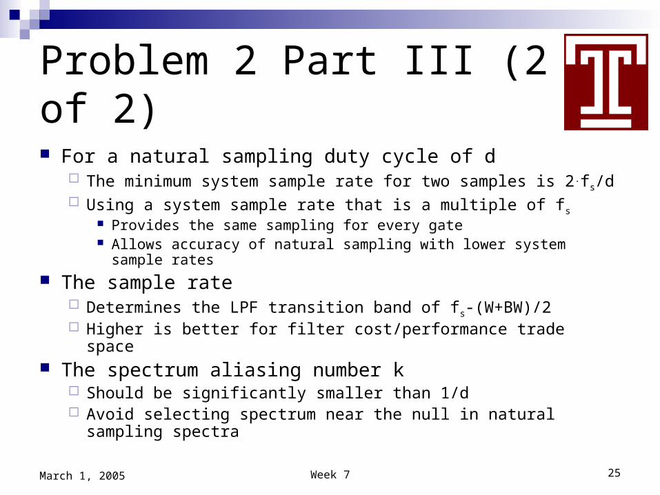
Problem 2 Part III (2 of 2)

For a natural sampling duty cycle of d The minimum system sample rate for two samples is 2.fs/d Using a system sample rate that is a multiple of fs

Provides the same sampling for every gate Allows accuracy of natural sampling with lower system sample rates

The sample rate Determines the LPF transition band of fs-(W+BW)/2 Higher is better for filter cost/performance trade space

The spectrum aliasing number k Should be significantly smaller than 1/d Avoid selecting spectrum near the null in natural sampling

spectra


Question 3 – The Block Diagram

Bandpass signal

Local Oscillator

LPF

Bx t

0exp 2j f t

1x t

Ox t22

2


Problem 3 Part I

The output signal xO(t) is the bandpass signal xB(t) shifted down in frequency by f0

For all-analog signals, the LPF Will supplement the last I.F. filter Can provide better performance than a bandpass filter

For sampled signals, the LPF Provides anti-aliasing filtering – suppression of

spectral images May allow decimation to sample rate near BW


Question 3, Part II

Considerations are similar to those of Question 2 In Question 2, natural sampling generated an array of

bandpass signals The complex rest of the circuit was a quadrature

demodulator that selected one of the bandpass signals

The duty cycle is not a part of Question 3 Minimum sample rate is 2.W LPF

Bandpass to BW/2 Stopband begins at fs – W/2


Problem 3 Part III

Sample rates fs that alias f0 to ±fs/4

Nyquist criteria, including spectral spread

Lowest sample rate is for a k of

04

2 1s

ff

k

2sf W

0 01 1ceiling floor

2 2

f fk

W W


Problem III Part IV

Look at numerical values of LPF specsBandpass to BW/2Stopband begins at fs – W/2

Transition band is fs-(BW+W)/2

Shape factor is (2.fs-W)/BW

LPF trade space is better for higher fs


Problem 3 Part V

The sample rate at I.F. is 2.W For complex signals, the Nyquist rate is W Allowing for a shape factor for the LPF increases the

sample rate above 2.W Decimation

Minimum is a factor of 2 to produce a sample rate of W complex Aliasing considerations can drive a complex data rate higher

than W Higher sample rates and simpler LPF will allow decimation of 3

or 4 to produce a complex sample rate near W Dual-stage digital LPF can provide a very high performance – a

shape factor only slightly larger than 1


SystemView

I have a mini-CD-ROM with the trial version When you install

During business hours When asked for “Regular” or “Professional” select

“Professional” Call Maureen Chisholm at 678-218-4603 to get your

activation code Other resources

The student version will probably carry you another week

The full version is available in E&A 604E – watch for two icons on the desktop and select the Professional version


Term Projects

Interpret, plan, model Use SystemView Assignments deployed by email last week Your preferences and comments are

encouragedOffice hoursEmail


SystemView Assignment

Objectives Generate test signal over speech band Determine fundamental simulation parameters

SystemView sample rate Run end time Comm system sample rate

Mimics Problem 3 Part V Successful completion is launch of your term

project


Term Project

Information

source

FormatSource encode

EncryptChannel encode

Multi-plex

Pulse modulate

Bandpass modulate

Freq-uency spread

Multiple access

X M I T

FormatSource decode

DecryptChannel decode

Demul-tiplex

DetectDemod-ulate & Sample

Freq-uency

despread

Multiple access

R C V

Channel

Information

sink

Bit stream

Synch-ronization

Digital baseband waveform

Digital bandpass waveformDigital

outputˆ im

Digital input

im

ˆiu z T r t

iu ig t is t

Optional

Essential

Legend:

Message symbols

Channel symbols

Channel symbols

From other

sources

To other destinations

Message symbols

Channel impulse

response

ch t


System


Spectrum of Input SignalSystemView

200

200

1.2e+3

1.2e+3

2.2e+3

2.2e+3

3.2e+3

3.2e+3-10

-30

-50

-70

-90

Powe

r Den

sity

Frequency in Hz (dF = 439.5e-3 Hz)

Spectral Density of Input (dBm/Hz 50 ohms)


Next Steps

Sample at comm system sample rate Adjust SystemView sample rate

Make it the comm system sample rate times a power of 2

This allows a power of 2 for both SystemView and comm system sampled data for the same run times

Quantize to 16 bits Convert to bitstream Map characters to 2-bit symbols for QPSK or

MSK


Sklar Chapter 4

Information

source

FormatSource encode

EncryptChannel encode

Multi-plex

Pulse modulate

Bandpass modulate

Fre-quency spread

Multiple access

X M I T

FormatSource decode

DecryptChannel decode

Demul-tiplex

DetectDemod-ulate & Sample

Freq-uency

despread

Multiple access

R C V

Channel

Information

sink

Bit stream

Synch-ronization

Digital baseband waveform

Digital bandpass waveformDigital

outputˆ im

Digital input

im

ˆiu z T r t

iu ig t is t

Optional

Essential

Legend:

Message symbols

Channel symbols

Channel symbols

From other

sources

To other destinations

Message symbols

Channel impulse

response

ch t


Detection

CoherentBPSKMPSKFSK

Non-coherentDifferential PSKFSK


Correlator Receiver

ir t s t n t N

0

T

ir t f t dt DECISIONLOGIC

is t

The correlation functions fi(t) may be Signal replicas si(t)

Orthogonal basis functions

With the right decision logic – a maximum likelihood detector


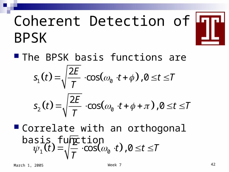
Coherent Detection of BPSK

The BPSK basis functions are

Correlate with an orthogonal basis function

1 0

2 0

2cos , 0

2cos , 0

Es t t t T

T

Es t t t T

T

1 0

2cos , 0t t t T

T


BPSK Demodulated Output

Output is plus or minus the pulse amplitude, depending on the phase

Coherence in this case lets us set the phase Φ to zero

Not knowing Φ Causes a fundamental ambiguityStill allows us to detect bit changes


Coherent MPSK Detection

M-ary PSK signals are

The basis functions are

0

2 2cos , 0 , 1, ,i

E is t t t T i M

T N

1 0

2 0

2cos , 0

2sin , 0

t t t TT

t t t TT


MPSK Demodulated Output

Output is a complex numberMagnitude is the pulse amplitudePhase is the modulation phase

Not knowing the phaseCauses a fundamental ambiguityStill allows us to detect phase changes


Coherent Detection of FSK

FSK waveforms are

We take the phase as zero, as before Basis functions are

2cos , 0 , 1, ,i i

Es t t t T i M

T

2cos , 0j jt t t T

T


Non-Coherent PSK Detection

Differential PSKUnknown phase of signal is a random variablePhases of adjacent received pulses are

compared Performance

Coherent – measure one phaseNon-coherent – measure two phases and

subtract Non-coherent is inherently noisier by 3 dB


Non-Coherent FSK

Use a filter bank Use I-Q demodulator Threshold the squared magnitudes


Example 4.1 pp. 187-188

Correlation is four-sample summation Waveform set is

Correlation is by summation over k

1

2

, 0

, 0

, 0,1,2,34k

s t A t t T

s t A t t T

Tt k k


Example 4.1 (Concluded)

Correlator summation is

What is z2?

2 232

10

14

4 4k

A Az k


Example 4.2 pp. 193-194

Phase as a function of propagation delay Phase changes by 360 degrees for each

wavelength of change of path length Wavelength for 1 GHz is about 1 foot Conclusion

Path length uncertainty of 3 inches will cause 90 degrees of phase uncertainty

Coherent detection depends on real-time monitoring of received phase

Phase-locked loops (PLLs) are needed to support coherent detection


Assignment

Add quantization and the ADC to your term project

Read Skar, sections 4.6, 4.7, 4.8, and 4.9 Look at symbol mapping for QPSK and

MSK for your term project Back-up quiz grades will be given by email

because next week is Spring Break

Documents

March 1, 2005Week 7 1 EE521 Analog and Digital Communications James K. Beard, Ph. D. [email protected] Tuesday, March 1, 2005 jkbeard