Mapping the exposure to natural disaster losses for ... · PDF fileMapping the exposure to natural disaster losses for Italian municipalities* ... assessment of full measures of economic

by

Giovanni Marin, Marco Modica

Mapping the exposure to natural disaster losses for Italian municipalities

SEEDS is an interuniversity research centre. It develops research and higher education projects in the fields of ecological and environmental economics, with a special focus on the role of policy and innovation. Main fields of action are environmental policy, economics of innovation, energy economics and policy, economic evaluation by stated preference techniques, waste management and policy, climate change and development.

The SEEDS Working Paper Series are indexed in RePEc and Google Scholar. Papers can be downloaded free of charge from the following websites: http://www.sustainability-seeds.org/. Enquiries:[email protected]

SEEDS Working Paper 09/2016 October 2016 by Giovanni Marin, Marco Modica

The opinions expressed in this working paper do not necessarily reflect the position of SEEDS as a whole.

http://www.sustainability-seeds.org/

mailto:[email protected]

1

Mapping the exposure to natural disaster losses for

Italian municipalities*

Giovanni Marin† Marco Modica

‡

Abstract

Even though the correct assessment of risks is a key aspect of the risk

management analysis, we argue that limited effort has been devoted in the

assessment of full measures of economic exposure at very low scale. For

this reason, we aim at providing a complete and detailed map of the

exposure of economic activities to natural disasters in the Italian context.

We use Input-Output model and spatial autocorrelation (Moran's I) to

provide information about several socio-economic variables, such as

population density, employment density, firms’ turnover and capital stock,

that can be seen as direct and indirect socio-economic exposure to natural

disasters. These measures can be easily incorporated into risk assessment

models to provide a clear picture of the disaster risk for Italian local areas.

Keywords: Economic exposure, Disaster impact; Risk assessment; Risk

management

* Authors acknowledge financial support from the research project "La valutazione economica dei disastri

economici in Italia" funded by the Fondazione Assicurazioni Generali. Usual disclaimer applies. † IRCrES-CNR, via Corti, 12, 20133 Milano, Italy; SEEDS Sustainability Environmental Economics and

Dynamics Studies, Ferrara, Italy. E-mail: [email protected] ‡ IRCrES-CNR, via Corti, 12, 20133 Milano, Italy; SEEDS Sustainability Environmental Economics and

Dynamics Studies, Ferrara, Italy. E-mail: [email protected]

2

1 Introduction

The perception about the relevance of economic and social damage generated by natural

disasters has grown substantially in recent decades (Blaikie et al., 2014). This greater

awareness about natural disasters triggered the demand, from both the public and the

private sectors, of actions aimed at preventing the occurrence of natural disasters (when

possible), at mitigating the damages and at adapting to increasing risks. On these

regards, a stronger collaboration of private and public sectors has gained on importance

through Public-Private Partnerships (PPPs) (Mysiak and Pérez-Blanco, 2015) due to

several reasons. First, climate change suggests that extreme events are likely to happen

in a more harsh way that in the past (DEFRA, 2013; Warner et al. 2013). Second, the

role of the governments in managing natural disasters implies a large and direct

financial burden because of the emergency relief, recovery, and reconstruction

(GFDRR, 2014). However, after the 2008 financial crises, the ability of governments to

finance interventions for disaster protection, recovery and reconstruction is in doubt

(Mysiak and Pérez-Blanco, 2015). Finally, the private insurance sector will not be able

to cover all the claims for damages in case of natural disasters (Botzen and Van Den

Bergh, 2012; Munich Re, 2009), especially so if they are due to global phenomena like

climate change. In the PPP context, information about risk and exposure to damages is

fundamental both in an ex-ante perspective (e.g. risk reduction, risk assessment) and in

the ex-post perspective (e.g. risk management, assessment of damage, reconstruction) to

allow for the correct definition of the role in the public and private partnership.

Even though the correct risk assessment is without any doubt a key aspect of the risk

management analysis, and for this reason the academic literature contains a large variety

of sophisticated models for risk assessment, we argue that less effort has been devoted

in the assessment of full measures of socio-economic exposure at very low scale. For

this reason, we aim at providing a complete and detailed map of exposure of socio-

economic activities to natural disasters in the Italian context. We provide detailed

information on several socio-economic variables that can be easily added to risk

assessment models to provide a clear picture of the disaster risk for any Italian local

areas. These variables are population density, employment density, firms’ turnover and

capital stock (divided also in its main component: buildings ad machineries).

In this respect, given the difficulties to address all the exposed goods, the existing

literature employs different proxies of the socio-economic exposure (Chen et al., 1997)

that depend on the features of the disaster that is analyzed. For instance, the density of

the built environment is a common proxy used in the case of flood risk assessment, (e.g.

Jongman et al., 2012; Koks et al., 2014, 2015: Sterlacchini et al., 2016). The Gross

Domestic Product, (GDP), or the population density are commonly used in earthquake

risk assessment (Chen et al., 1997), as well as the value of real estate assets (Field et al,

2005; Meroni et al., 2016). A similar proxy can be used in the case of drought (land

value, Simelton et al., 2009) while for landslides an interesting measure is the mix

3

between social (population), physical (buildings and infrastructures), economic (land

value) and environmental (site of community importance) indicators (Bloechl and

Braun, 2005; Pellicani et al., 2014).

The different choice of the proxy used in the evaluation of the economic losses due to

natural disasters mostly depends on the sequence of effects which are expected to occur

when different natural disasters affect a given area (Modica and Zoboli, 2016; Pelling,

2003). On these regards, there is extensive literature focusing on the definition of losses

caused by extreme events (see ECLAC, 2003; FEMA, 1992; and Pelling et al., 2002, for

more details). Even though definitions are not always coherent among each other, for

simplicity we discriminate between direct and indirect losses.

Direct losses refer to direct damages to people (injuries and fatalities) and objects

(goods, buildings, infrastructures, etc.), ECLAC (2003). For instance, earthquakes

destroy buildings and infrastructure, which in turns, generate damages to other goods

and people. Floods may generate minor damages to buildings if compared to damages

to other goods (e.g. vehicles) and people (FFEMA 2003; Luino et al., 2009). Damages

arising from the interruption of economic activities due to the natural disaster are also

considered to be direct losses (see Rose and Lim, 2002; Rose et al, 2007). Interruption

may occur for several reasons: damages to critical infrastructures such as energy and

water supply and transport network; damages to people involved in production

processes, destruction of production capital, etc. The interruption of economic activities

in a region reduces the firms’ turnover for a certain amount of time, which in turn

reduces region’s GDP.

A second category of losses includes indirect losses. This category is broad and

borderless. Limiting the discussion to the indirect consequences of business

interruption, foregone production and turnover also influences the whole (local and

global) supply chain of the production activities that experience the interruption (e.g.

Van Der Veen and Logtmeijer, 2005). Suppliers of intermediate goods will have a

reduction in the demand for their products and consequently a reduction in turnover. On

the other hand, customers will experience potential shortage of inputs needed for their

production process and may be forced to find alternative suppliers, thus increasing

production costs and potentially reducing production. Foregone wages will also

influence region’s GDP as consumption will be reduced. Finally, if the interruption lasts

for a long period, producers may lose their customers permanently, limiting the

possibility of economic recovery even once the cause of interruption is removed. For all

these reasons indirect losses need to be evaluated looking at general equilibrium effects

by means of specific economic models, however this is not an east task (see Okuyama,

2007).

Given these premise it turns out that policy makers and private actors have the vital

need to know both the direct and indirect components of economic exposure for the

elaboration and implementation of correct and effective risk management strategies.

Direct components refer to those that might produce direct losses as a consequence of

4

the disaster, from now on 'direct socio-economic exposure'. Indirect components refer to

the losses due to the disruption of local and global supply chains of the production

activities as a consequence of the disaster ('indirect socio-economic exposure'). Indeed,

policy makers need to know clearly what is the socio-economic value of the area under

analysis, as well as the possible interconnections between neighboring areas, to define

for instance optimal mitigation policies in selected risky prone areas or to estimate the

likely (or potential) maximum cost suffered by a region affected by a disaster. Private

actors, such as insurance companies, can instead uses this information to provide a more

accurate risk analysis and to provide better insurance plans.

However, measuring the costs and the economic impacts of extreme events is a difficult

task due to the unpredictability of the different types of natural events (Hallegatte and

Przylusky, 2010), both in the ex-ante and in the ex-post perspective, also for the scarcity

of information about economic activities for small geographical units. To overrule this

issue we create a set of maps of several socio-economic measures that can be used in

different contexts and in relation to several natural disasters at a very detailed scale,

providing in this way a full map of the potential exposure of socio-economic activities

to natural disasters in the Italian municipalities.

Using administrative and statistical data we estimate a set of socio-economic

information that can be used to map the socio-economic exposure of geographical unit

in terms of direct economic exposure. The complete set of measures that we provide are

the following: population density (proxy for potential life loss), employee density

(indirect measure of how exposed is a municipality during its ‘working hours’),

turnover (direct costs due to business interruption) and capital stock (direct costs due to

the destruction of capital goods). These measures provide interesting information on the

direct exposure since they are all proxy for the ‘local’ loss of the area due to natural

disasters.

In order to consider the indirect socio-economic exposure, we also provide relevant

information on the spatial clustering of the socio-economic characteristics underlined

above, by means of local indicator of spatial autocorrelation (LISA), (for details see

Anselin, 1995 and for an application see Cutter and Finch, 2008). This analysis is useful

to identify areas where high values are spatially concentrated at municipality level,

indicating in this way a greater economic exposure to risk and potentially high indirect

losses. Finally, we also provide more explicit evidence about local linkages and possible

diffusion of economic damages by means of input-output inter-sectoral linkages across

neighboring municipalities.

These maps can inform risk assessment models to provide a robust tool for the risk

management at different administrative levels (municipalities, regions, national

government) or to provide important information on local exposure per se.

The work is organised as follows. Section 2 describes data sources. Section 3 explains

the methodology used to attribute turnover and capital stock measures to local units.

5

Section 4 provides some descriptive evidence on the exposure to natural disasters of

socio-economic activities in Italian municipalities. Section 5 concludes.

2 Data sources

The main source of information that is employed to evaluate the exposure to natural

disasters of socio-economic activities in Italian municipalities is the ASIA database of

Istat (Archivio Statistico delle Imprese Attive). "ASIA - Imprese" includes detailed

information on the population of Italian companies from 1996 to 2012. This information

includes the address of the headquarter of the firm, the number of employees, the class

of turnover, the main sector of the firm (5-digit NACE) and its unique identifier. The

total number of firms in 2011 was 4,515,691 firms and they were distributed across

different classes of turnover as described in Table 1.

Table 1 – Distribution of firms by turnover class (in euro)

Class Min Max # firms

1 0 19,999 1,042,223

2 20,000 49,999 1,161,047

3 50,000 99,999 788,529

4 100,000 199,999 603,462

5 200,000 499,999 464,785

6 500,000 999,999 198,311

7 1,000,000 1,999,999 120,353

8 2,000,000 3,999,999 66,543

9 4,000,000 4,999,999 13,791

10 5,000,000 9,999,999 28,355

11 10,000,000 19,999,999 14,312

12 20,000,000 49,999,999 8,487

13 50,000,000 199,999,999 4,230

14 200,000,000 1,263

This detailed information is very relevant but it is still characterized by two main

limitations for the aim of providing an appropriate estimate of 'local' turnover. First, the

'true' value of turnover for each firm is unknown as we only know the turnover class of

the firm. While for some classes the range is rather narrow, in some other cases

(especially so for classes with greater turnover) the range is very wide. To illustrate, the

upper bound estimate (the true value of turnover of all firms within a class equals the

maximum of the class) is about 2.42 times greater than the lower bound estimate (the

true value of turnover of all firms within a class equals the minimum of the class), even

excluding the top class (turnover greater than 200 million euro),. Moreover, the highest

class accounts for as much as 20 percent of total turnover, in the lower bound estimate.

This is particularly worrisome as no upper limit exists for this class.

A second reason of concern refers to the fact that many firms, especially the larger ones,

produce great part of their turnover in establishments other than the headquarter. In fact,

6

in single-unit firms all production occurs in the headquarter, while for multi-unit firms

(e.g. multi-plant) large share of production occurs in units other than the headquarter.

However, it is important to know where the production actually occurs for measuring

the exposure of a firm's production (and, consequently, turnover) to natural disasters. In

order to attribute the total turnover of the firm to its various branches (local units) we

combine "ASIA - Imprese" with "ASIA - Unità Locali" (local units). This latter

database contains information on the population of local units of Italian firms from 2004

to 2012. Similarly to "ASIA - Imprese", it contains the address of the local unit, the

number of employee, the main sector of the local unit (NACE 5-digit) and the unique

identifier of the firm. The total number of local units of Italian firms is 4,826,882 in

2011. Table 2 shows some descriptive statistics on the number of local units per firm,

split by turnover class. While small (in terms of turnover) firms have a very small

number of local units (around 1), larger firms have higher number of local units.

Proportionally distributing total firm production across different local units of the firms,

may result in a substantial over-estimation of the turnover generated in the municipality

of the headquarter and in a underestimation of the turnover generated in the

municipalities of the local units, especially so for large firms. Indeed, headquarters are

more likely to locate in big urban areas (e.g. Milan, Rome), therefore, the use of firm-

level data only would result in a systematic over-estimation of turnover (but also

employment and capital stock) in big urban areas.

To overrule these issues, the two sources of information described above have been

complemented with data on ‘true’ turnover at firm-level from the AIDA database

(Bureau van Dijk). This information is available only for 733,458 firms (16.24% of

total). However, these firms are responsible for 41.77% of total employees as AIDA

over-represents large firms. This is particularly important as big firms account for a

large share of turnover and having detailed (and ‘true’) information on these large

players limits the risk of systematically over-estimating or under-estimating turnover.

This over-representation of large firms is also apparent when looking at the share of

firms available in AIDA (over the total number of firms) by turnover class (

Table 3). While for small turnover classes the share of firms available in AIDA is very

small, the coverage of AIDA increases substantially for medium-large firms (up to

76.45% for firms in class 11).

7

Table 2 – Number of local units per firm by turnover class

Class Mean Q1 Median Q3 Max

1 1.02 1 1 1 239

2 1.01 1 1 1 28

3 1.02 1 1 1 21

4 1.05 1 1 1 37

5 1.11 1 1 1 65

6 1.19 1 1 1 146

7 1.29 1 1 1 173

8 1.43 1 1 2 190

9 1.59 1 1 2 133

10 1.84 1 1 2 380

11 2.42 1 1 2 838

12 3.41 1 2 3 546

13 7.71 1 2 5 1,599

14 42.42 2 5 14 12,392

Total 1.09 1 1 1 12,392

Table 3 – Distribution of firms available in AIDA by turnover class

Class

Firms in

AIDA (share

of total)

1 3.70%

2 3.78%

3 6.73%

4 12.38%

5 25.47%

6 40.75%

7 51.78%

8 62.08%

9 59.34%

10 73.48%

11 76.45%

12 72.33%

13 62.98%

14 55.50%

To estimate the value of the capital stock owned by economic activities, we retrieve

information on net stock of capital by sector at the national level (Investimenti fissi

lordi, stock di capitale e ammortamenti per branca proprietaria by Istat). This is

available for 37 sectors (sub-section, Ateco 2007 / NACE rev 2) until 2012. We retrieve

information on net capital stock (which is already partialled out from the depreciation of

capital) at the aggregate level as well as its various components: buildings, machinery,

intangibles. This information will be useful to estimate the expected stock of capital at

the municipality level given its local sectoral composition and the national average

capital stock per employee for each sector (see section 3.2). Finally, population density

has been provided by 2011 Italian Census of Istat.

8

3 Methodology

3.1 Estimates of turnover

A first step to estimate total turnover at the municipality level consists in estimating

firm-level turnover. As discussed in the previous section, actual turnover (from AIDA)

is available for a small number of firms while for the rest of firms we only have

information on the turnover class. To estimate firm-level turnover we fit an interval

regression model on the population of firms in which the log of turnover (in class or,

when available in AIDA, actual turnover) is function of the log of the number of

employees of the firm. The interval regression model is a generalisation of the Tobit

model in which both interval data and point data are allowed. After estimating the

model, we predict the turnover (given the level of employment). We substitute the

predicted turnover with the 'true' turnover from AIDA (when available) and we set to

the upper bound of the interval the predicted turnover whenever it exceeds the upper

bound. Similarly, we set the predicted turnover to the lower bound whenever it is

smaller than the lower bound.

The model is estimated separately for each industry (NACE Subsection) separately to

account for industry-specific relationship between employment and turnover.

Table 4 – Estimated turnover by turnover class (in billion euro)

Class Total turnover Share of total

Total turnover

(firms in

AIDA)

Share of

turnover in

firms in AIDA

1 18.53 0.58% 0.32 1.74%

2 40.40 1.26% 1.48 3.66%

3 49.80 1.55% 3.87 7.77%

4 73.96 2.30% 10.85 14.67%

5 124.68 3.88% 38.85 31.16%

6 124.24 3.87% 57.77 46.50%

7 151.75 4.73% 88.19 58.12%

8 170.69 5.31% 116.21 68.08%

9 59.46 1.85% 36.47 61.34%

10 186.71 5.81% 145.18 77.76%

11 190.28 5.92% 152.43 80.11%

12 243.32 7.58% 184.87 75.98%

13 355.65 11.07% 237.03 66.65%

14 1,422.13 44.28% 602.79 42.39%

Table 4 reports the estimated turnover by turnover class as well as the total turnover of

firms for which actual turnover was available in the AIDA database. A large share of

total turnover is estimated to be generated by large firms: firms belonging to the two top

classes of turnover account for more than 55% of total turnover. Moreover, the share of

turnover retrieved from AIDA (i.e. 'true' turnover) is greater in big turnover classes.

9

A final step of the analysis consists in attributing the total turnover of the firm to its

local units. We assume that the ratio between turnover and employees is constant within

each firm ( ) and consequently attribute firm-level turnover ( ) to local units (j)

according the share of employment of the local unit ( ) over the total employment of

the firm ( ).

(1)

Total turnover at the municipality level (m) is finally computed as the sum of estimated

turnover of local units operating in the municipality.

(2)

While total turnover by municipality is already useful as an indicator of exposure, it is

important to scale it by the total land size of the municipality, thus obtaining the average

turnover per square kilometre. This scaling factor is required as natural disasters

(earthquakes, floods, landslides) hit specific areas of land.

The indicator measures the average expected loss of turnover if economic activity is

completely interrupted for a year in a square kilometre of the municipality. The

indicator can be further refined to reflect the expected loss of turnover due to partial

interruption (e.g. 50%) or temporary (e.g. 7 days) interruption.

A final consideration is needed as forgone production and turnover in a specific local

unit may be compensated, at least partly, by greater production and turnover in other

local units in areas not affected by the potential natural disaster. This may occur within

the same multi-units firm or in units belonging to other firms. For this reason, the

indicator of turnover per square kilometre is a good indicator of the ‘local’ loss of

turnover due to the interruption of economic activity but it is an upper bound of overall

loss.

3.2 Estimates of capital stock

To estimate the net stock of capital of economic activities at municipality level we

assume that the ratio between capital stock and number of employees is homogeneous

in all Italian firms that belong to a specific sector (k). Table 5 shows the average national

capital intensity (net capital stock per employee in 2011) by industry. We observe very

large heterogeneity across industries in terms of capital intensity both for total capital

stock and for the different categories of capital goods. Real estate activities (L) have a

very high capital intensity which is mainly driven by its large stock of capital in

buildings. Its value is about 34 times the average value of all sectors. Capital stock in

machinery is less concentrated but still rather heterogeneous across sectors. Machinery

per employees in the two top industries (C19 and D) is about 13 times the average value

of all sectors. This great systematic heterogeneity across sectors in terms of capital

10

intensity is likely to explain a large part of the difference in capital intensity across local

units belonging to different sectors.

According to this assumption, the estimated capital stock for municipality m is given

by:

(3)

where is the total employment in local units in municipality m and sector k while

. This means that the only source of variation across municipalities is the

industry composition of economic activities of the municipalities. As discussed for

turnover, we scale the capital stock by the land size of the municipality.

The indicator reflects the average expected loss in capital stock if all productive capital

is destroyed in a square kilometre of land. As discussed for turnover, this can be refined

to reflect partial destruction.

11

Table 5 – Capital per employee by sector for Italy (source: Istat, year 2011)

Ateco Ateco (description)

Net capital stock

per employee Employees

Total Buildings Machinery Intangibles

C10T12 Manufacture of food products; beverages and tobacco products 0.1307 0.0423 0.0839 0.0046 425,548

C13T15 Manufacture of textiles, wearing apparel, leather and related

products 0.0578 0.0189 0.0327 0.0063 484,529

C16T18 Manufacture of wood, paper, printing and reproduction 0.0988 0.0321 0.0634 0.0033 292,733

C19 Manufacture of coke and refined petroleum products 1.6376 1.1378 0.4913 0.0084 18,947

C20 Manufacture of chemicals and chemical products 0.3121 0.1159 0.1663 0.0300 109,262

C21 Manufacture of basic pharmaceutical products and

pharmaceutical preparations 0.2613 0.0499 0.1518 0.0596 61,075

C22_23 Manufacture of rubber and plastic products and other non-

metallic mineral products 0.1411 0.0480 0.0876 0.0055 371,893

C24_25 Manufacture of basic metals and fabricated metal products,

except machinery and equipment 0.1182 0.0391 0.0752 0.0039 658,675

C26 Manufacture of computer, electronic and optical products 0.1807 0.0439 0.0784 0.0584 107,595

C27 Manufacture of electrical equipment 0.1301 0.0365 0.0746 0.0189 161,329

C28 Manufacture of machinery and equipment n.e.c. 0.1022 0.0381 0.0482 0.0158 452,592

C29_30 Manufacture of motor vehicles, trailers, semi-trailers and of

other transport equipment 0.1646 0.0261 0.0903 0.0482 259,434

C31T33 Manufacture of furniture; jewellery, musical instruments, toys;

repair and installation of machinery and equipment 0.0836 0.0455 0.0316 0.0065 436,062

D Electricity, gas, steam and air conditioning supply 2.4922 1.9940 0.4773 0.0209 87,915

E Water supply; sewerage, waste management and remediation

activities 0.3306 0.2105 0.1171 0.0030 182,310

F Construction 0.0549 0.0369 0.0173 0.0007 1,549,374

G Wholesale and retail trade; repair of motor vehicles and

motorcycles 0.0604 0.0425 0.0161 0.0018 3,446,704

H Transportation and storage 0.2972 0.2161 0.0785 0.0025 1,078,439

I Accommodation and food service activities 0.0905 0.0773 0.0129 0.0003 1,323,844

J58T60

Publishing, motion picture, video, television programme

production; sound recording, programming and broadcasting

activities

0.2280 0.1059 0.0390 0.0831 93,817

J61 Telecommunications 0.4205 0.2496 0.1025 0.0683 94,234

J62_63 Computer programming, consultancy, and information service

activities 0.0666 0.0147 0.0148 0.0371 354,460

K Financial and insurance activities 0.1495 0.1317 0.0090 0.0088 589,682

L Real estate activities 9.7985 9.7822 0.0140 0.0023 289,175

M69T71

Legal and accounting activities; activities of head offices;

management consultancy activities; architectural and

engineering activities; technical

0.0324 0.0207 0.0071 0.0046 912,709

M72 Scientific research and development 0.5844 0.3931 0.0814 0.1099 23,227

M73T75 Advertising and market research; other professional, scientific

and technical activities; veterinary activities 0.0499 0.0335 0.0116 0.0048 257,690

N Administrative and support service activities 0.0743 0.0431 0.0293 0.0018 1,114,627

P Education 0.4183 0.3411 0.0295 0.0477 90,519

Q86 Human health activities 0.1827 0.1460 0.0270 0.0098 483,403

Q87_88 Residential care activities and social work activities without

accommodation 0.0522 0.0439 0.0066 0.0018 272,135

R Arts, entertainment and recreation 0.2383 0.1699 0.0377 0.0274 173,595

S Other service activities 0.0641 0.0497 0.0120 0.0023 449,108

Total 0.2908 0.2466 0.0370 0.0072 16,706,641

4 Descriptive evidence

In this section we provide some descriptive evidence on the exposure to natural

disasters of socio-economic activities in 8,056 Italian municipalities for year 2011. The

variables that we have selected as proxy for socio-economic exposure to natural

disasters are population density, employment density, turnover and capital stock

(divided also for its components: capital on buildings ad machineries). Indeed,

12

according to Dilley (2005, p.31) “to understand the risks posed by a range of hazards, it

is also essential to characterize the exposure of people and their economic activities to

the different hazards. Ideally, we would have a complete probability density function for

population exposure to specific types of events...such estimates might vary depending on

the time of the day, day of the week or month of the year”.

Population density based on place of residence is a proxy for potential life loss across

different types of hazards (Dilley, 2005). However, because of commuting for work

reasons, we also use employment density as an indirect measure of how exposed is a

municipality during its ‘working hours’.

To capture the exposure of economic activities, we instead focus on turnover and capital

stock of firms. Turnover provides a measure of the gross economic value produced by

an area in one year and it might be considered as the potential direct cost suffered by the

area due to business interruption. Instead, capital stock reflects the average expected

loss in buildings and machinery if all productive capital is completely destroyed in a

square kilometre of land.

All these measures per se are able to provide information on the components that are

directly exposed to natural disasters and that could cause direct losses. In order to

account for the indirect effects induced by natural disasters in a given area, we have to

account also for the dependency of each industry in a given municipality to all other

industries in neighboring municipalities to retrieve intermediate inputs and as a market

for final goods and service.

In the following of this section we first evaluate how the measures correlate each other.

Then we look at the geographical distribution of proposed indicators and. we discuss the

maps for the clustering of municipalities. Finally, we discuss our measures of indirect

economic exposure.

4.1 Correlation across measures

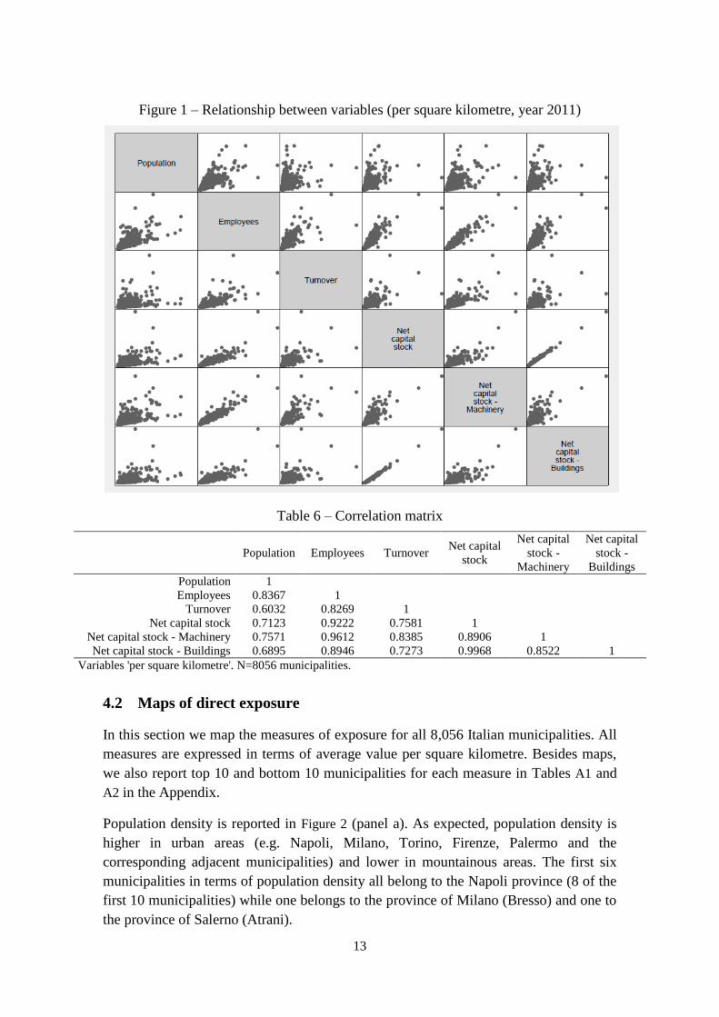
Figure 1 and Table 6 report, respectively, the bivariate relationships and the correlation

matrix between our measures of exposure to natural disasters. All measures are highly

correlated. Correlation however is far from perfect between capital stock (and its

components) and employment despite the former is estimated by using information of

the latter. This means that heterogeneity in capital intensity across sectors and

differences in sectoral composition across municipalities is substantial and results in

rather heterogeneous estimates of exposure of productive capital stock. The greatest

correlation is between total capital stock and capital stock in buildings (which

represents a large share of the total capital stock), while the smallest correlation is

between population and turnover.

13

Figure 1 – Relationship between variables (per square kilometre, year 2011)

Table 6 – Correlation matrix

Population Employees Turnover

Net capital

stock

Net capital

stock -

Machinery

Net capital

stock -

Buildings

Population 1

Employees 0.8367 1

Turnover 0.6032 0.8269 1

Net capital stock 0.7123 0.9222 0.7581 1

Net capital stock - Machinery 0.7571 0.9612 0.8385 0.8906 1

Net capital stock - Buildings 0.6895 0.8946 0.7273 0.9968 0.8522 1

Variables 'per square kilometre'. N=8056 municipalities.

4.2 Maps of direct exposure

In this section we map the measures of exposure for all 8,056 Italian municipalities. All

measures are expressed in terms of average value per square kilometre. Besides maps,

we also report top 10 and bottom 10 municipalities for each measure in Tables A1 and

A2 in the Appendix.

Population density is reported in Figure 2 (panel a). As expected, population density is

higher in urban areas (e.g. Napoli, Milano, Torino, Firenze, Palermo and the

corresponding adjacent municipalities) and lower in mountainous areas. The first six

municipalities in terms of population density all belong to the Napoli province (8 of the

first 10 municipalities) while one belongs to the province of Milano (Bresso) and one to

the province of Salerno (Atrani).

14

When considering employees per square kilometre (Figure 2,panel b) we observe some

relevant difference. Employment seems to be more concentrated in large cities. At the

same time, surrounding municipalities of large cities appear now less dense than when

considering population. This reflects the fact that many people commutes from sub-

urban municipalities to the urban centre to work. Looking at the first ten municipalities,

we now observe a predominance of municipalities that belong to the province of Milano

(5) followed by the province of Napoli (3).

Turnover instead follows the common Italian pattern of economic growth being more

concentrated in Northern Italy rather than in the Southern part of the country (Figure 3,

panel a). The Lombardy, in general, and metropolitan area of Milan, in particular, look

the more relevant areas. Indeed if we focus on the first ten municipalities ranked by

turnover, eight over ten are in the metropolitan area of Milan, while the other two are in

Lombardy.

Moving to total capital stock (Figure 3, panel b), we observe that its value is rather high

also for medium-sized urban centres in the northern part of Italy (Padova, Bologna,

Bergamo, Brescia, Genova) as well as municipalities in the northern part of the Adriatic

coast. Among the top 10, municipalities in the province of Milano still lead (5).

As a large share of the total capital stock is composed by buildings, the distribution of

our measure of capital stock in building is very similar to the one of total capital (Figure

4, panel a).

The stock of capital in machinery is mostly concentrated in municipalities which are

specialised in industrial production (Figure 4, panel b). Again, 6 municipalities of the top

10 are located in the province of Milano.

To sum up, descriptive evidence highlights a rather heterogeneous exposure of

municipalities to natural disasters. However, the correlation between the various

measures is very high and exposure according to different metrics tend to be overlapped

to a great extent.

15

(a) Population density (per square kilometre, year 2011) (b) Employees (per square kilometre, year 2011)

Figure 2 – Direct exposure of population and employees

16

(a) Turnover (per square kilometre, year 2011) (b) Net capital stock - Total (per square kilometre, year 2011)

Figure 3 – Direct exposure of turnover and total capital stock

17

(a) Net capital stock - Buildings (per square kilometre, year 2011) (b) Net capital stock - Machinery (per square kilometre, year 2011)

Figure 4 – Direct exposure of capital stock in buildings and machinery

18

4.3 Maps of indirect exposure

4.3.1 Spatial statistics

As a last step of descriptive evidence, we evaluate some geographical features of our

measures of exposure. For all variables of interest we estimate the spatial

autocorrelation (Moran's I, Moran, 1950) using as geographical weights either the

contiguity matrix which considers only direct neighbours (first column) or the

contiguity matrix that considers up to the fifth group of neighbours. The Moran’s I is

computed as:

(4)

Results are reported in Table 7. Spatial autocorrelation is rather high for population

density, employee density and capital stock (total and its various components) per

square kilometre, while it is rather low for turnover. Spatial correlation is much greater

when using one-neighbours spatial weights than when using five-neighbours spatial

weights.

Table 7 – Spatial autocorrelation (Moran’s I)

Variable Moran’s I

1 neighbour

Moran’s I

5 neighbours

Population 0.728 0.266

Employees 0.695 0.236

Turnover 0.087 0.040

Net capital stock – Total 0.540 0.169

Net capital stock – Buildings 0.505 0.152

Net capital stock – Machinery 0.638 0.245

Net capital stock - Intangible 0.571 0.170

4.3.2 Clustering

We compute Local Indicators of Spatial Associations (LISA, see Anselin, 1995). For

each municipality we compute the local Moran’s I (based on the 5-neighbours

weighting matrix) and identify clusters of municipalities and outliers. Whenever the

local Moran’s I is not statistically different from zero the municipality does not belong

to a cluster and it is not an outlier (light grey area). On the other hand, four possible

outcomes are possible when the local Moran’s I is statistically significant:

the municipality belongs to a clusters with high values (HH, red area);

the municipality belongs to a cluster with low values (LL, blue area);

the municipality is an outlier with high value surrounded by municipalities with

low value (HL, pink area);

19

the municipality is an outlier with low value surrounded by municipalities with

high value (LH, light blue area).

This approach is particularly useful as it allows to easily identify possible hot-spots or

critical areas in terms of exposure to natural disasters. If a cluster ‘HH’ belongs to a

region characterized by high probability of experiencing a natural disaster, that will

generate large damages no matter the specific municipality (or municipalities) is

directly affected as most municipalities in the region have high values of exposure. On

the contrary, ‘LL’ clusters in regions with high probability of experiencing a natural

disaster will experience rather low average expected damages as economic activities are

not concentrated in any of the municipalities of the clusters. Finally, ‘HL’

municipalities belonging to areas with high risk of natural disasters will be

characterized by a very high expected damage which is combined, however, to a rather

low probability of being the municipality that is hit among the ones belonging to the

larger region.

Results for population, employment, turnover, total capital stock, capital stock in

buildings and capital stock in machinery are shown in Figure 5, Figure 6 and Figure 7.

For what concerns population (Figure 5, panel a), we observe HH clusters in medium-

large urban areas (Milano, Torino, Genova, Bergamo, Padova, Firenze, Prato, Rimini,

Roma, Pescara, Napoli, Bari, Palermo and Cagliari, among others) while LL clusters

emerge in the mountains of Alps and Appennini. Few HL outliers also exists in

correspondence of medium towns while LH outliers are very uncommon. Evidence for

employment density (Figure 5, panel b) is very similar to what is found for population

while for turnover (Figure 6, panel a) we observe a much smaller number of (smaller)

HH clusters. Finally, the various measure of capital stock (Figure 6, panel b, and Figure

7) tend to reflect to a great extent what we found for employment.

20

(a) Local Moran's I for population density (year 2011) (b) Local Moran's I for employees density (year 2011)

Figure 5 – Clustering for population and employees

21

(a) Local Moran's I for turnover density (year 2011) (b) Local Moran's I for net total capital stock density (year 2011)

Figure 6 – Clustering for turnover and total capital stock

22

(a) Local Moran's I for net capital stock in buildings density (year

2011)

(b) Local Moran's I for net capital stock in machinery density (year

2011)

Figure 7 – Clustering for capital stock in buildings and machinery

23

4.3.3 Socio-economic exposure to the damage of the nearby municipalities

The evaluation of spatial clustering based on direct exposure to risk is an implicit way

of assessing indirect exposure to risk. The link between neighbouring municipalities

with similar (high or low) exposure may indicate some sort of economic linkage

between the municipalities. Even though proximity is often endogenous and driven by

agglomeration forces that enable to take advantage of geographically concentrated

economic linkages, a more explicit measure of economic linkage is needed.

At a more aggregate level, the economic literature has focused on inter-sectoral (input

output) relationships as a mechanism through which shocks diffuse throughout the

economy (Acemoglu et al., 2012). The general idea is that, especially in the short run,

the collapse of a sector (due to any reason, including natural disasters) has an impact on

other sectors that are either upstream (suppliers) or downstream (customers) in the

supply chain. If, for any reason, the output of a sector experiences an unexpected drop,

firms in that sector will respond by reducing their demand for intermediate goods from

upstream sectors. Suppliers, in turn, will also reduce their production as one of their

customer sectors has reduced its demand. Moreover, a collapse in the production of a

sector will also generate shortages (at least in the short run) of inputs for those sectors

that need goods or services produced by the collapsed sector (i.e. downstream sectors).

These shortages induce a slow down (or even an interruption) of the production

activities of the downstream sectors.

Even though approaches based on input–output modeling have been criticized for some

weaknesses (i.e. rigid structure and lack of responses to price changes, see Rose, 2004),

they have been widely used in the assessment of disaster damages, mostly because of

their attitude to capture the economic interdependencies within a regional economy

(Okuyama, 2014). For instance Tan et al. (2015) use IO to estimate the maximum

percentage of damage that an economic system is able to absorb. Rose and Wei (2013)

simulate the impact of a seaport shutdown to the national economy through input-output

while Van Der Veen and Logtmeijer (2005) simulate the impact of a large-scale

flooding in one province of Netherlands.

To translate this approach to the local level (e.g. municipality), a number of

assumptions need to be made. First, statistical agencies, with very few exceptions, only

provide national input-output tables. This means that it is not possible to account for

likely geographic heterogeneity in technical coefficients. Even though these coefficients

generally reflect rather standard 'recipes' for producing final goods, heterogeneity exists

and cannot be accounted for. More importantly, a second assumption refers to the share

of inputs that a firm purchases from local suppliers and to the share of output that a firm

sells to local customers. National input-output tables are split into a 'domestic'

transaction table and a 'rest of the world' transaction table. In absence of any

information about the relevance of local suppliers and customers, we use the national

domestic input-output table that represents an upper-bound of the relevance of local

suppliers. The implicit assumption, in fact, is that all 'national' inputs are completely

24

purchased from firms in neighbouring municipalities. Even though this is a very strong

assumption, the absence of information about cross-regional and cross-municipal trade

flows limits the possibility of providing any better estimate of the share of 'local'

sourcing of intermediates over total 'national' sourcing of intermediates. A third

assumption relates to the definition of 'local' linkages, namely how far should be the

municipality affected by natural disasters to influence other cities (Östh et al., 2016). To

evaluate the sensitivity of our mapping to this assumption we report results for two

different thresholds of distance (e.g. 20 km and 50 km). Finally, the diffusion of shocks

influences, as a first step, only direct suppliers and customers. However, the shock also

propagates to suppliers of suppliers and customers of customers. To simplify, in our

analysis we only consider 'first order' effects and leave the evaluation of higher order

effects (e.g. using the Leontief model for suppliers and the Ghoshian model for

customers) for future research.

We therefore build two different measures. The first measures the share of output

(turnover) created in a municipality that can be absorbed by firms that operate in

neighbouring municipalities as intermediate inputs, within a certain distance (either

20km or 50km). We first compute the total output by sector in the municipalities within

the radius of the reference municipality. These totals are then post-multiplied to the

technical coefficient matrix of the input-output matrix (i.e. the matrix A, that describes

the amount of euro of goods that are required from each sector j to produce one euro of

goods for sector i). We obtain, in this way, the hypothetical demand of intermediate

inputs from each sector in neighbouring municipalities. We then divide this hypothetical

demand by the output (of each sector) produced in the municipality of reference and

take the average across sectors (weighted by the turnover of each sector). This measure

indicates the relative share of inputs that neighbouring municipalities may potentially

purchase from companies in the municipality of reference. We define this measure as

"Destination of final output in neighbouring municipalities". This measure captures the

potential lack of goods in the neighbouring municipalities due to a shock in production

(eventually driven by a natural disaster) that occurs in the municipality of reference.

This may undermine production activities in neighbouring municipalities and determine

an indirect loss also in case the disaster only affects the municipality of reference.

Results are reported in Figure 8. To ease the graphical representation, we rescaled the

indicator to be in a range between 0 and 1. Figure 8 does not show a well defined

pattern. What is interesting to note, however, is that at the top of the list we have both

municipalities that host large industrial facilities (i.e. the steel districts of Piombino and

Taranto) and large cities (e.g. Rome, Milan, Palermo, Turin).

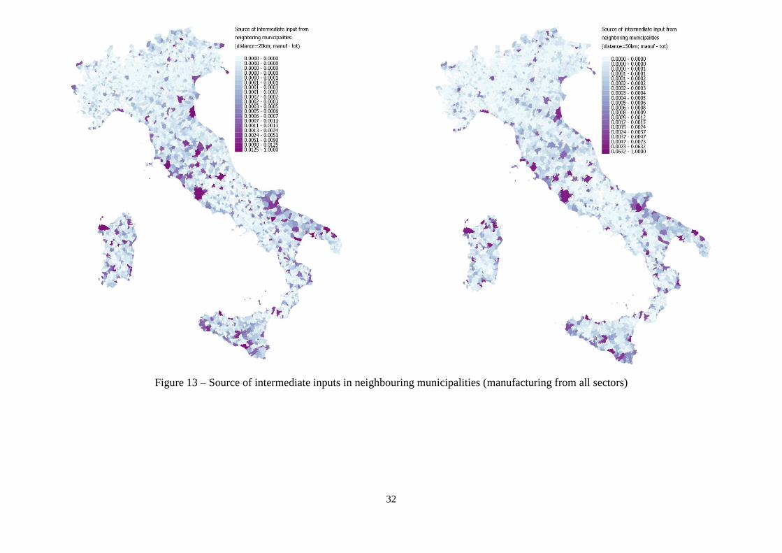
Similarly, we compute the share of intermediate inputs that can be possibly retrieved

locally (i.e. in neighbouring municipalities) by firms that operate in the municipality of

reference. We post-multiply the vector of total turnover by sector of the municipality of

reference by the technical coefficient matrix to obtain the potential demand for

intermediate inputs from firms in the municipality. We then divide each element of this

25

vector by the vector of total production (turnover) by sector in neighbouring

municipalities and take averages across sector (weighted by the turnover of each sector).

This measure proxies the potential share of inputs that can be retrieved by firms in the

municipality of reference from firms that operate in neighbouring municipalities. We

define this measure as "Source of intermediate inputs in neighbouring municipalities".

The measure is useful to quantify the potential drop in demand (for intermediates) that

could be experienced by neighbouring municipality in the case a disaster interrupts

production in the municipality of reference.

Results are reported in Figure 9. Also in this case, to ease the graphical representation,

we rescale the indicator to be in a range between 0 and 1. Even though the list of

municipalities at the very top remain the same (i.e. industry-based municipalities and

large cities), the correlation with the previously discussed measure (Figure 8) is positive

but not very large (0.45), thus suggesting that these measures depict different

dimensions of indirect exposure.

Results should be interpreted as follows: the overall density of activities (of any sector)

in large cities generates a large demand for intermediate inputs, that usually is above the

output produced in neighbouring municipalities. On the other hand, manufacturing

sector (such as steel industries) are characterized, on average, by much larger 'upstream'

multipliers (or, in our case, technical coefficients) than service sectors as they require a

large amount of intermediate inputs to carry out production activities. This generates a

large demand for intermediates that often cannot be completely met by neighbouring

municipalities, leading to high values for our indicators.

Not all sectors are likely to be influenced (directly and indirectly) by natural disasters in

the same way. On the one hand, manufacturing sectors are, on average, more capital

intensive than service sectors. In case the natural disaster under evaluation has relevant

consequences in terms of destruction of capital goods, capital intensive sectors are more

likely to be forced to interrupt their production activities than less capital intensive

sectors. On the other hand, given that manufacturing sectors are 'tradable' sectors (i.e.

they are exposed to foreign competition). Tradability implies that there is the risk that

temporary interruptions in production due to the disaster induce a permanent change in

the structure of the supply chain in favour of manufacturing firms operating in other

areas.

For these reasons, we also provide evidence for manufacturing-to-manufacturing

linkages as well as manufacturing-to(from)-all sectors linkages. These measures are

reported in Figure 10, Figure 11, Figure 12 and Figure 13. While providing a full

discussion of the results for these alternative measures goes beyond the aim of the

paper, it is interesting to observe that these measures positively correlate each other

even though this correlations is usually far from perfect (see Table 8)

26

Table 8 – Correlation across measures of indirect exposure

Destination of final output in neighbouring municipalities (20 km radius)

Tot-Tot Manuf-Tot Manuf-Manuf

Tot-Tot 1

Manuf-Tot 0.58 1

Manuf-Manuf 0.59 0.98 1

Source of intermediate inputs in neighbouring municipalities (20 km radius)

Tot-Tot Manuf-Tot Manuf-Manuf

Tot-Tot 1

Manuf-Tot 0.73 1

Manuf-Manuf 0.68 0.88 1

27

Figure 8 – Destination of final output in neighbouring municipalities (all sectors)

28

Figure 9 – Source of intermediate inputs in neighbouring municipalities (all sectors)

29

Figure 10 – Destination of final output in neighbouring municipalities (manufacturing to manufacturing)

30

Figure 11 – Destination of final output in neighbouring municipalities (manufacturing to all sectors)

31

Figure 12 – Source of intermediate inputs in neighbouring municipalities (manufacturing to manufacturing)

32

Figure 13 – Source of intermediate inputs in neighbouring municipalities (manufacturing from all sectors)

33

5 Conclusion

Very few effort has been devoted until know to addressing the most appropriate socio-

economic values for determining exposure to natural disasters in an ex-ante perspective

and in assessing the cost suffered by local areas in an ex-post perspective. This study is,

to our knowledge, an attempt of moving toward this direction. We have used

administrative and statistical data to estimate a set of economic information that can be

employed to map the potential economic exposure of narrowly defined geographical

units (e.g. municipalities) in terms of direct and indirect socio-economic consequences

of natural disasters. These types of maps can be integrated into existing and emerging

models for risk assessment or as benchmark for urban planning, risk mitigation policies

and risk prevention.

Besides providing estimates of direct socio-economic exposure to natural disasters, we

also develop and compute different measures of indirect socio-economic exposure.

These indicators are particularly useful to quantify the overall potential economic

impact of natural disasters on specific areas, also beyond the boundaries of the location

that is directly affected by natural disasters. Our results show that even though all

indicators (direct and indirect exposure) are positively correlated, due to structural

differences across municipalities (mostly in terms of density of population and

economic activities), these correlations are far from perfect and suggest that differences

in the economic structure of municipalities may result in different transmission of

shocks to neighboring municipalities as a consequence of natural disasters.

The approach developed in this study as well as the type of data that are employed may

be particularly useful for academic and policy-relevant evaluations of risk assessment

and damage cost evaluation of natural disasters, from both an ex-ante and ex-post

perspective. The indicators we propose could be further refined to account for the

specificities of the case study for which they are employed. It could be useful, for

example, to geo-reference all economic activities of a narrowly defined area (i.e.

smaller than the administrative boundaries of a municipality), to use more detailed

information about the distance between the municipality of reference and the economic

activities that could potentially suffer from indirect damages or, finally, to select a

reduced number of sectors due to their higher or lower exposure to direct or indirect

damages.

34

References

Acemoglu D, Carvalho VM, Ozdaglar A, Tahbaz-Salehi A (2012) The Network Origins

of Aggregate Fluctuations. Econometrica, 80(5), 1977–2016.

Anselin L (1995) Local Indicators of Spatial Association – LISA. Geographical

Analysis, 27(2):93–115.

Blaikie P, Cannon T, Davis I, Wisner B. (2014).At risk: natural hazards, people's

vulnerability and disasters. Routledge

Bloechl A, Braun B (2005). Economic assessment of landslide risks in the Swabian Alb,

Germany‒research framework and first results of homeowners' and experts' surveys.

Natural Hazards and Earth System Science, 5(3), 389–396.

Botzen WJ, Van Den Bergh JC (2012). Monetary valuation of insurance against flood

risk under climate change. International Economic Review, 53(3), 1005–1026.

Chen QF, Chen Y, Liu JIE, Chen L (1997). Quick and approximate estimation of

earthquake loss based on macroscopic index of exposure and population distribution.

Natural Hazards, 15(2–3), 215–229.

Cutter S.L, Finch C (2008). Temporal and spatial changes in social vulnerability to

natural hazards. Proceedings of the National Academy of Sciences. 105, 2301–2306

DEFRA (2013) Securing the future availability and affordability of home insurance in

areas of flood risk. Report of Department for Environment, Food and Rural Affairs

Dilley M (2005). Natural disaster hotspots: a global risk analysis (Vol. 5). World Bank

Publications.

ECLAC (2003). Handbook for Estimating the Socio-economic and Environmental

Effects of Disasters, United Nations Economic Commission for Latin America and the

Caribbean

FEMA (1992). Indirect Economic Consequences of a Catastrophic Earthquake, edited

by: Milliman, J.W. and Sanguinetty, J. A., National Earthquake Hazards Reduction

Program

Field EH, Seligson HA, Gupta N, Gupta V, Jordan TH, Campbell KW (2005). Loss

estimates for a Puente Hills blind-thrust earthquake in Los Angeles, California.

Earthquake Spectra, 21(2), 329–338.

GFDRR (2014) Financial protection against natural disasters. An operational

framework for disaster risk financing and insurance. International Bank for

Reconstruction and Development / International Development Association or The

World Bank

35

Hallegatte S, Przylusky V (2010). The economics of natural disasters. Concepts and

Methods, Policy Research Working Paper 5507

Jongman B, Kreibich H, Apel H, Barredo JI, Bates PD, Feyen L, Ward PJ (2012).

Comparative flood damage model assessment: towards a European approach. Natural

Hazards and Earth System Science 12(12), 3733–3752.

Koks EE, de Moel H, Aerts JC, Bouwer LM (2014). Effect of spatial adaptation

measures on flood risk: study of coastal floods in Belgium. Regional environmental

change, 14(1), 413–425.

Koks EE, Jongman B, Husby TG, Botzen WJW (2015). Combining hazard, exposure

and social vulnerability to provide lessons for flood risk management. Environmental

Science & Policy, 47, 42–52.

Luino F, Cirio CG, Biddoccu M, Agangi A, Giulietto W, Godone F, Nigrelli G (2009).

Application of a model to the evaluation of flood damage. Geoinformatica, 13(3), 339–

353.

Meroni F, Pessina V, Squarcina T, Locati M, Modica M, Zoboli R (2016). The

economic assessment of seismic damage: an example for the 2012 event in Northern

Italy presented at ICUR2016 (forthcoming)

Mysiak JCD, Pérez-Blanco CD, (2015) Partnerships for Affordable and Equitable

Disaster Insurance , Nota di Lavoro 40.2015, Milan, Italy: Fondazione Eni Enrico

Mattei.

Modica M, Zoboli R (2016). Vulnerability, resilience, hazard, risk, damage, and loss: a

socio-ecological framework for natural disaster analysis, Web Ecology, 16, 59–62,

Moran PAP (1950). Notes on Continuous Stochastic Phenomena. Biometrika, 37(1):17–

23.

Munich Re (2009). From knowledge to solutions. Solvency II, Climate change. Munich

Re.

Okuyama Y (2007). Economic Modeling for Disaster Impact Analysis: Past, Present,

and Future. Economic Systems Research, 19(2):115–124.

Okuyama Y, Santos JR (2014). Disaster Impact and Input–Output Analysis, Economic

Systems Research, 26:1, 1–12

Östh J, Lyhagen J & Reggiani A (2016). A new way of determining distance decay

parameters in spatial interaction models with application to job accessibility analysis in

Sweden, European Journal of Transport and Infrastructure Research, 16(2):344–363

Pellicani R, Van Westen CJ, Spilotro G (2014) Assessing landslide exposure in areas

with limited landslide information. Landslides, 11(3), 463–480.

36

Pelling M (2003). The Vulnerability of Cities: Natural Disasters and Social Resilience,

Earthscan, London.

Pelling M, Ozerdem A, Barakat S (2002). The macro-economic impact of disasters.

Progress in Development Studies, 2, 283–305

Rose, A. (2004). Economic Principles, Issues, and Research Priorities in Hazard Loss

Estimation. In: Y. Okuyama and S.E. Chang (eds.) Modeling Spatial and Economic

Impacts of Disasters. NewYork, Springer, 13–36.

Rose A, Lim D (2002) Business interruption losses from natural hazards: conceptual

and methodological issues in the case of the Northridge earthquake. Environmental

Hazards, 4(1):1–14.

Rose A, Oladosu G, Lia SY (2007) Business Interruption Impacts of a Terrorist Attack

on the Electric Power System of Los Angeles: Customer Resilience to a Total Blackout.

Risk Analysis, 27(3):513–531.

Rose A, Wei D (2013). Estimating the Economic Consequences of a Port Shutdown:

The Special Role of Resilience, Economic Systems Research, 25:2, 212–232,

Simelton E, Fraser ED, Termansen M, Forster PM, Dougill AJ (2009). Typologies of

crop-drought vulnerability: an empirical analysis of the socio-economic factors that

influence the sensitivity and resilience to drought of three major food crops in China

(1961–2001). Environmental Science & Policy, 12(4), 438–452.

Sterlacchini S, Zazzeri M, Genovese E, Modica, M, Zoboli R (2016). Flood damage in

Italy: towards an assessment model of reconstruction costs, EGU General Assembly

2016, held 17-22 April, 2016 in Vienna Austria, p.13135

Tan RR, Aviso KB, Promentilla MAB, Solis FDB, Yu KDS, Santos JR (2015) A Shock

Absorption Index For Inoperability Input–Output Models, Economic Systems Research,

27:1, 43–59

Van Der Veen A, Logtmeijer C (2005) Economic Hotspots: Visualizing Vulnerability to

Flooding. Natural Hazards, 36:65–80.

Warner K, Yuzva K, Zissener M, Gille S, Voss J, Wanczeck S (2013).Innovative

Insurance Solutions for Climate Change: How to integrate climate risk insurance into a

comprehensive climate risk management approach. UNU-EHS.

37

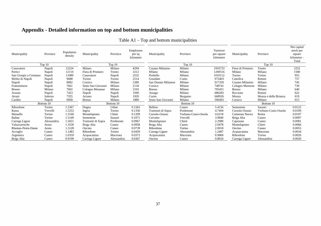
Appendix - Detailed information on top and bottom municipalities

Table A1 – Top and bottom municipalities

Municipality Province Population

density Municipality Province

Employees per sq

kilometre

Municipality Province Turnover per square

kilometre

Municipality Province

Net capital

stock per square

kilometre -

Total

Top 10

Top 10

Top 10

Top 10

Casavatore Napoli 12224

Milano Milano 4294

Cusano Milanino Milano 1916733

Fiera di Primiero Trento 2252

Portici Napoli 12110


Milano Milano 1269516

Milano Milano 1580

San Giorgio a Cremano Napoli 11089


Pioltello Milano 1010112

Torino Torino 955 Melito di Napoli Napoli 9688

Torino Torino 2514

Grandate Como 975403

Cattolica Rimini 757

Napoli Napoli 8082

Corsico Milano 2389

San Donato Milanese Milano 917359


Frattaminore Napoli 7661

Sesto San Giovanni Milano 2134

Corsico Milano 748741

Cologno Monzese Milano 730 Bresso Milano 7602

Cologno Monzese Milano 2103

Bresso Milano 705451

Bresso Milano 640

Arzano Napoli 7423

Napoli Napoli 1949

Assago Milano 686283

Riccione Rimini 622

Atrani Salerno 7355

Arzano Napoli 1920

Curno Bergamo 668926

Monza Monza e della Brianza 619 Cardito Napoli 6958

Bresso Milano 1889

Sesto San Giovanni Milano 596493

Corsico Milano 615

Bottom 10

Bottom 10

Bottom 10

Bottom 10

Ribordone Torino 1.5367

Dogna Udine 0.1563

Bellino Cuneo 5.4156

Semestene Sassari 0.0122 Rassa Vercelli 1.5253

Ingria Torino 0.1356

Tramonti di Sopra Pordenone 4.7404

Cursolo-Orasso Verbano-Cusio-Ossola 0.0109

Massello Torino 1.5160

Montelapiano Chieti 0.1209


Camerata Nuova Roma 0.0107

Balme Torino 1.5149

Semestene Sassari 0.1071

Cervatto Vercelli 3.9840

Briga Alta Cuneo 0.0097

Carrega Ligure Alessandria 1.5021

Tramonti di Sopra Pordenone 0.0967


Caprauna Cuneo 0.0081

Valsavarenche Aosta 1.3530




Rhemes-Notre-Dame Aosta 1.3128

Oncino Cuneo 0.0739


Oncino Cuneo 0.0055 Acceglio Cuneo 1.1483



Acquacanina Macerata 0.0034

Argentera Cuneo 1.0359






Oncino Cuneo 0.8024


38

Table 9 – Top and bottom municipalities (by type of capital good)


Net capital stock per square

kilometre -

Buildings


Net capital stock per square

kilometre -

Machinery

Top 10

Top 10



Milano Milano 1404

Milano Milano 134

Torino Torino 837


Cattolica Rimini 721




Riccione Rimini 598

Pomigliano d'Arco Napoli 94


Corsico Milano 91

Monza Monza e della Brianza 559

Torino Torino 86

Lissone Monza e della Brianza 553

Pero Milano 85

Bresso Milano 546

San Donato Milanese Milano 84

Bottom 10

Bottom 10


Canosio Cuneo 0.0027

Pramollo Torino 0.0080

Perlo Cuneo 0.0027

Camerata Nuova Roma 0.0074






Oncino Cuneo 0.0045



Oncino Cuneo 0.0008







Documents

Mapping the exposure to natural disaster losses for ... · PDF fileMapping the exposure to natural disaster losses for Italian municipalities* ... assessment of full measures of economic