188

Wea

ther

– Ju

ly 20

10, V

ol. 6

5, N

o. 7

Mapping Manchester’s urban heat islandSylvia Knight1, Claire Smith2 and Michael Roberts3

1Royal Meteorological Society, Reading 2University of Manchester3Altrincham Grammar School for Girls, Cheshire

IntroductionAn urban heat island (UHI) is a phenomenon whereby urban areas experience elevated temperatures relative to the surrounding rural hinterland. This thermal contrast is brought about by anthropogenic modifica-tion of the environment. For example, there is little bare earth and vegetation in urban areas. This means that less energy is used in evaporating water, less of the Sun’s energy is reflected and more heat is stored by buildings and the ground in urban than in rural areas. The heat generated by heating, cooling systems, transport and other energy uses also contributes, particularly in winter, as does the complex three-dimensional structure of the urban landscape which can reduce air flow.

The magnitude of the urban-rural tem-perature difference depends upon a range of meteorological and geomorphological variables, but the maximum UHI is generally observed under night-time, calm, clear-sky conditions following a day of similar weather. In this scenario, the lack of cloud means daytime solar radiation receipt is at its great-est, leading to a large component of stored heat in the urban fabric. This heat is later released into the surrounding environment as the external air temperature drops after sunset. Meanwhile, net longwave radiation losses are at a maximum during the evening in rural areas but remain comparatively low in the city owing to higher levels of air pollution and radiation becoming trapped by tall urban structures. When the wind is light, nocturnal cooling is inhibited by the lack of available ventilation to transport the warmer air away from the urban environ-ment, further accentuating the difference. The alteration of the urban radiative energy balance and the reduction of heat loss by

wind-driven turbulence in a city environ-ment are both consequences of the urban surface geometry.

Although complex, the relationship between urban morphology and the urban-rural temperature difference has been shown to display an inverse linear association under the idealised UHI conditions outlined above for a range of mid-latitude, devel-oped, cities (Oke, 1981). Spatial temperature variations within a city, however, may not correspond quite so simply with building height and/or density owing to other factors that are present at the microscale (Eliasson, 1996). For instance, a key difference in the surface energy budget is in the ratio of latent to sensible heat fluxes. In rural areas the surface is dominated by evapotranspir-ing vegetation, but in an urban environ-ment much of the surface has undergone some level of waterproofing through the use of impervious materials, thereby signifi-cantly reducing the latent heat flux (Grimmond and Oke, 1999; 2002).

Differences in land use, irrigation, wind speed and rainfall mean that evaporative cooling varies within urban environments. On a local scale, the presence of a vegetated area or water body within a city can have a significant cooling effect (Spronken-Smith and Oke, 1999; Graves et al., 2001). Temperature patterns are dominated by an inverse relationship between temperature and distance from the city centre, but are also strongly related to land use, which is often a surrogate for urban morphology, geometry and the availability of water (Landsberg, 1981; Eliasson and Svensson, 2003; Wilby, 2003).

The significance of UHIs was brought to the attention of city planners and the wider public by the heatwave of August 2003. In London, for example, night-time tempera-tures were six to nine degrees higher than in the surrounding countryside during the heatwave. This contributed to an estimated 600 excess deaths (Mayor of London, 2006). Buildings and transport infrastructure, which typically have a long life cycle, are not designed to withstand such extreme temperatures, as the UHI effect is generally not considered during the design process. Consequently, when heatwaves are exacer-

bated by the UHI, the infrastructure can be subject to over-heating, structural damage, changed energy consumption patterns and disrupted service provision. Increasing urban development and population com-pounded by projected temperature changes, mean that the resulting economic costs will be significant unless the UHI effect is considered in future design. The detailed structure of UHIs must therefore be quantified.

While the causes of the UHI are generally well understood (Landsberg, 1981; Oke, 1987), it is often difficult to quantify the magnitude and spatial variation of the effect due to the lack of standardised long-term meteorological observations in urban areas and the sparse network of monitoring stations. In the UK, studies of UHIs have tended to focus on London (Wilby, 2003; Mayor of London, 2006; Jones and Lister, 2009), although limited data also exist for Reading (Parry, 1955; Melhuish and Pedder, 1998) and Birmingham (Unwin, 1980). The aim of a project currently underway at the University of Manchester (SCORCHIO: Sustainable Cities: Options for Responding to climate CHange Impacts and Outcomes), in partnership with the University of Sheffield, University of Newcastle, University of East Anglia and the Hadley Centre is to develop a suite of Geographic Information System (GIS)-based decision-support tools which will allow for the analysis of climate change adaptation options in urban areas, with a particular emphasis on heat and human comfort. As part of this work, a detailed picture of the spatial temperature patterns across Greater Manchester is being developed (Kilsby et al., 2007; Smith et al., 2010). The results collected so far suggest a maximum Manchester UHI effect of ~3 degC during the day which increases to 5 degC at night (Smith et al., 2010).

The RMetS Big Urban Heat Island ExperimentIn 2008, the Education Committee of the Royal Meteorological Society initiated a campaign to map the urban heat islands of several UK cities and towns. The aims of this campaign are to:

189

Weather – July 2010, Vol. 65, No. 7

Mapping M

anchester’s UHI

• Create a database of good quality, local measurements that schools could use, as UHIs feature in many GCSE and A-level specifications.

• Involve students and the public in col-lecting data, thereby raising awareness and understanding of the UHI effect.

• Collect data that could be of use to research groups and city planners;

• Raise the profile of the Society amongst schools and the general public.

The Society will initiate UHI measurement campaigns in one UK urban area at a time, with a view to establishing what the maxi-mum heat island effect might be under idealised heat island conditions, and what the spatial structure of the UHI might be. In each case, the Society will work closely with local research groups and schools.

To maximise the numbers of partici pants, it was decided to allow temperature meas-urements to be made using car thermome-ters. After consulting the European Automobile Manufacturers’ Association, as well as conducting a number of experi-ments, these were found to be reasonably accurate, providing readings were only made after the vehicle had been moving at some speed for a number of minutes. When moving, the thermometers are not affected by engine heat; they display current, rather than archived, temperatures. If the numbers of participants are sufficient, random errors in these thermometers can be accounted for. On the morning selected for each inves-tigation, participants are invited to drive to their destination, and then immediately text the outside temperature reading and post-code of their destination to a specified

number. It can then be assumed that the time of the text corresponds to the time of the temperature measurement.

In addition, several hundred simple digital thermometers with a precision of 0.1 degC and an accuracy of ±1% (manufacturer’s specification – this is typical for cheap digital thermometers) were purchased for distribu-tion to schools in the selected areas. This significant variability meant that each one had to be numbered and an offset applied to any readings made. It was also found that, due to slow reaction speeds, the thermom-eters had to be left outside overnight prior to any reading. We requested that thermom-eters be left at least three metres from any building and about one metre from the ground, but this was not always possible.

In November 2008, a trial experiment was carried out in Reading. Poor weather

From the lead school’s point of viewIt was midway through the typically busy autumn term when we were invited to get involved in the UHI project. Without appreciat-ing what we were taking on, we sprang into action to create a management group mainly of sixth-form students. We also had enthusiastic staff involvement as the Head of sixth-form teaches Geography and one of the sixth-form tutors is Head of Science. Our students saw the project as an opportunity to be involved in a major piece of research, something which they would be doing in a few years time at university – great for their CVs/personal statements.

As a lead school it became apparent that we would need to involve the local community to take the all-important temperature measurements. The students took on the job of contacting and involving local primary schools, with many returning to their old schools. To get the general public involved, the students, supported by a member of our office staff who has a responsibility for the media, started to contact newspapers, radio and TV stations. Some good coverage came from local newspapers with visits from a couple of photographers all wanting that special shot of a group of students taking the air temperature! Our first batch of 30 thermometers had arrived and it became apparent that they recorded a range of temperatures. The discerning students spotted this and had to be reas-sured that the experiment would be valid as the instruments would be adjusted with an offset based on the average reading.

As Christmas approached, meetings took place almost daily. We had a comprehensive master plan to work from, all focused on the day selected to take the temperatures. How could we get the thermometers out to primary schools wanting to take part? When would the next batch of 190 thermometers arrive? How would we get to know what day had been selected? How would we inform the rest of the school to collect these thermometers? Which students would be prepared to speak to pupils in assemblies? What would we do with the readings? Would we cover a large enough area? Could we get more media coverage and hence more readings?

We returned after the Christmas break to a week of almost perfect weather for the experiment. A high pressure system produced cold, clear mornings but the thermometers were still in transit. When the 190 thermometers arrived, we quickly got onto the job of numbering them and determining the offset data. This was done by leaving them overnight in a science prep. room and recording the temperatures next morning. Typically we were getting temperatures of around 18°C– after all this was indoors! The question was then asked Is the offset linear? Should we not be taking the offset readings at much lower temperatures? To answer these questions all 190 thermometers ended up overnight in the back of my campervan. Early next morning two students braved the cold and quickly recorded the temperatures. Now we had some accurate figures to give a reliable offset reading – all good science!

The day selected for the temperature readings took us by surprise: nevertheless, we were ready! On the preceding day, lower-school students queued to be allocated their thermometers and the slip of paper on which they would record the thermometer number, location, time and temperature. Our media contacts started to come good with BBC Radio Manchester wanting to put in a live link to their morning show and BBC TV wanting to follow the action including filming one of our year 10 pupils at home, recording her early morning temperature readings. Our Head of Sixth Form and Head of Science volunteered to take a couple of students out in their cars to record temperatures on major routes around the city.

We had decided to make the data collection a bit more exciting than simply handing in a bit of paper. As pupils and staff brought in their results, coloured dots were placed on a large-scale map of the area by our sixth-form team (Fig. 1). Whilst this was all going on, BBC Radio Manchester was interviewing students and staff about the project and taking calls from around Manchester from other members of the public. At about 0830 UTC the BBC TV Film crew arrived to follow the proceedings and to interview students and staff involved in the project. The resulting footage and commentary shown at midday and in the evening proved to be excellent with some well-informed reporting by the presenters (BBC, 2009a; 2009b).

By midday the exhausted members of the team co-ordinating the project were satisfied that they had given it their best shot hav-ing managed to obtain over 300 temperatures. When combined with readings taken by the general public we hoped that the results would be worthwhile and valid. Certainly, one of the highlights was the excellent media coverage from both radio and TV. This cover-age has recently been extended with our students being invited to contribute to a follow-up feature on BBC Radio Manchester. On reflection the team recognised that the whole exercise was not just about making a contribution to scientific research and to raising public awareness but about project management – that alone made it worthwhile.

190

Wea

ther

– Ju

ly 20

10, V

ol. 6

5, N

o. 7

Map

ping

Man

ches

ter’s

UHI

conditions, with a warm front passing through during the period of the experi-ment, meant that the results generated were not good enough to be published. Many valuable lessons were learnt, however.

Typically the temperature difference between rural and urban areas is larger at night than during the day, is most obvious when winds are weak and skies are clear, and is greater in the summer than in the winter (Oke, 1987). We attempt to pick times and conditions when the UHI effect is max-imised so that the relationship between land use and temperature is as easy to detect as possible, allowing the structure of the UHI to be clearly seen. The timing of the experiment is also restricted by the need to be on a weekday in term time, to allow school participation, and by the need to allow measurements at a time when a sig-nificant number of people would be awake. Therefore, we require as late a sunrise as possible. It was decided that suitable weather conditions should be identified 48 hours in advance, to allow local media and all those involved to be contacted. This meant that Mondays were also not suitable.

We planned to carry out a measurement campaign in Manchester in January in con-junction with SCORCHIO. Given the con-straints, it was actually March before the 48-hour weather forecast suggested that a clear, calm night could reasonably be expected on 6 March. By this time, sunrise was at 0644 UTC and most measurements would be made after the sun had affected air temperature.

Greater Manchester has a population of over 2.5 million people. It is a landlocked county covering 1276 square kilometres lying mostly below 100 metres above sea level, with more significant changes in alti-tude at the far eastern edge of the urban area, where the Cheshire Plain meets the Pennines. The effect of altitude on tempera-ture could therefore be expected to be smaller than the random errors introduced by the choice of thermometers for most of the area studied. Greater Manchester is an interesting case study as it incorporates a wide range of land-use types with differing surface cover, built form and socio-eco-nomic characteristics.

All Heads of Geography in secondary schools in Greater Manchester received a letter inviting them to participate in the experiment, to which several responded, some requesting thermometers. Altrincham Grammar School for Girls became the lead school for the campaign.

ResultsAlthough the pressure remained high through the night of 5/6 March (Figure 2) and the skies were clear through the early

cally have experienced rapid cooling due to the openness of the environment and the lack of obstruction to outgoing radiation.

Over 1000 data points were collected, com-prising 304 texts sent in by the general pub-lic, 320 measurements collected by school students across Manchester and other data including time series collected from vari-ous weather stations (including relevant sta-tions supplying data to the Climatological

Figure 1. A small group of girls from Altrincham Grammar School for Girls was key to publicising the experiment throughout their school, to primary schools in the local area and to the local media. They collected measurements from students as they came to school and plotted them on an OS map.

Figure 2. Surface analysis chart for 0000 UTC on 6 March 2009, showing a ridge of high pressure over Manchester at the time of the measurements.

part of the night, by 0600 UTC a thick layer of stratocumulus had formed, but with an extensive break over central Manchester. In practical terms, this meant that the light air-craft available to the SCORCHIO group was not able to supplement the campaign with airborne measurements. In terms of the UHI effect, such cloud could be expected to insulate the ground, reducing the rate of nocturnal heat loss from the Earth’s surface, particularly in rural areas which would typi-

191

Weather – July 2010, Vol. 65, No. 7

Mapping M

anchester’s UHI

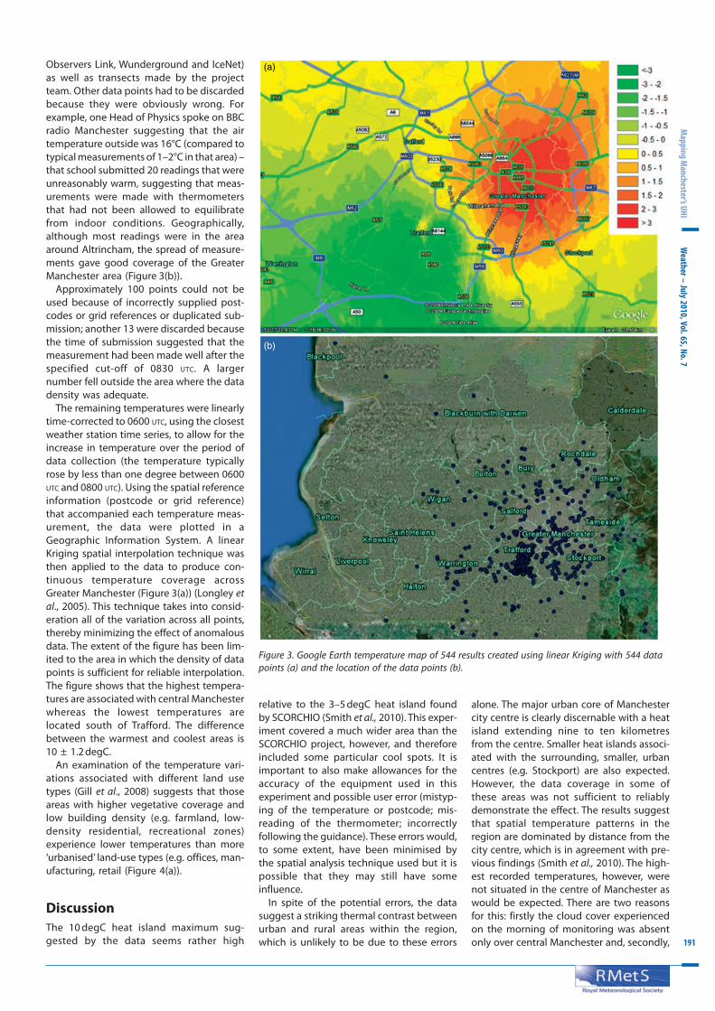
Observers Link, Wunderground and IceNet) as well as transects made by the project team. Other data points had to be discarded because they were obviously wrong. For example, one Head of Physics spoke on BBC radio Manchester suggesting that the air temperature outside was 16°C (compared to typical measurements of 1–2°C in that area) – that school submitted 20 readings that were unreasonably warm, suggesting that meas-urements were made with thermometers that had not been allowed to equilibrate from indoor conditions. Geographically, although most readings were in the area around Altrincham, the spread of measure-ments gave good coverage of the Greater Manchester area (Figure 3(b)).

Approximately 100 points could not be used because of incorrectly supplied post-codes or grid references or duplicated sub-mission; another 13 were discarded because the time of submission suggested that the measurement had been made well after the specified cut-off of 0830 UTC. A larger number fell outside the area where the data density was adequate.

The remaining temperatures were linearly time-corrected to 0600 UTC, using the closest weather station time series, to allow for the increase in temperature over the period of data collection (the temperature typically rose by less than one degree between 0600 UTC and 0800 UTC). Using the spatial reference information (postcode or grid reference) that accompanied each temperature meas-urement, the data were plotted in a Geographic Information System. A linear Kriging spatial interpolation technique was then applied to the data to produce con-tinuous temperature coverage across Greater Manchester (Figure 3(a)) (Longley et al., 2005). This technique takes into consid-eration all of the variation across all points, thereby minimizing the effect of anomalous data. The extent of the figure has been lim-ited to the area in which the density of data points is sufficient for reliable interpolation. The figure shows that the highest tempera-tures are associated with central Manchester whereas the lowest temperatures are located south of Trafford. The difference between the warmest and coolest areas is 10 ± 1.2 degC.

An examination of the temperature vari-ations associated with different land use types (Gill et al., 2008) suggests that those areas with higher vegetative coverage and low building density (e.g. farmland, low-density residential, recreational zones) experience lower temperatures than more ‘urbanised’ land-use types (e.g. offices, man-ufacturing, retail (Figure 4(a)).

DiscussionThe 10 degC heat island maximum sug-gested by the data seems rather high

relative to the 3–5 degC heat island found by SCORCHIO (Smith et al., 2010). This exper-iment covered a much wider area than the SCORCHIO project, however, and therefore included some particular cool spots. It is important to also make allowances for the accuracy of the equipment used in this experiment and possible user error (mistyp-ing of the temperature or postcode; mis-reading of the thermometer; incorrectly following the guidance). These errors would, to some extent, have been minimised by the spatial analysis technique used but it is possible that they may still have some influence.

In spite of the potential errors, the data suggest a striking thermal contrast between urban and rural areas within the region, which is unlikely to be due to these errors

(a)

(b)

Figure 3. Google Earth temperature map of 544 results created using linear Kriging with 544 data points (a) and the location of the data points (b).

alone. The major urban core of Manchester city centre is clearly discernable with a heat island extending nine to ten kilometres from the centre. Smaller heat islands associ-ated with the surrounding, smaller, urban centres (e.g. Stockport) are also expected. However, the data coverage in some of these areas was not sufficient to reliably demonstrate the effect. The results suggest that spatial temperature patterns in the region are dominated by distance from the city centre, which is in agreement with pre-vious findings (Smith et al., 2010). The high-est recorded temperatures, however, were not situated in the centre of Manchester as would be expected. There are two reasons for this: firstly the cloud cover experienced on the morning of monitoring was absent only over central Manchester and, secondly,

192

Wea

ther

– Ju

ly 20

10, V

ol. 6

5, N

o. 7

Map

ping

Man

ches

ter’s

UHI

ReferencesBBC. 2009a. How warm is Manchester? http://www.bbc.co.uk/manchester/content/articles/2009/02/04/040209_hot_manchester_feature.shtml [Accessed 6 March 2009.]BBC. 2009b. Pupils join climate survey. http://news.bbc.co.uk/1/hi/england/7929584.stm [Accessed 6 March 2009.]Eliasson I. 1996. Urban nocturnal temperatures, street geometry and land use. Atmos. Environ. 30: 379–392.Eliasson I, Svensson MK. 2003. Spatial air temperature variations and urban land use – a statistical approach. Meteorol. Appl. 10: 135–149.Gill SE, Handley JF, Ennos AR, Pauleit S, Theuray P, Lindley SJ. 2008. Characterising the urban environment of UK cities and towns: a template for landscape planning in a changing climate. Landscape Urban Plan. 87: 210–222.Graves H, Watkins R, Westbury P, Littlefair P. 2001. Cooling buildings in London: Overcoming the heat island. BRE and DETR: London.Grimmond CSB, Oke TR. 1999. Heat storage in urban areas: local-scale observations and evaluation of a simple model. J. Appl. Meteorol. 38: 922–940.

there were relatively few measurements within Manchester city centre.

It is difficult to establish which parameters are important on a more localised scale due to the non-uniform data coverage, but using a land-use classification scheme (Gill et al., 2008) we are able to draw some general conclusions: the variation of temperature across the different land-use types (Figure 4) is encouragingly similar to the findings of the SCORCHIO project (Smith et al., 2010). In particular, land-use types with high build-ing density and energy consumption (imply-ing large amounts of waste heat), for example manufacturing areas and offices, are found to experience comparatively high temperatures. In general, these areas also have minimal vegetative surface cover, which implies that latent cooling through

evapotranspiration is significantly reduced compared to areas with a higher proportion of vegetative cover. The relatively lower temperatures recorded in greener land-use types (e.g. farmland, recreation) are also indicative of the importance of vegetative cover for cooling the local environment (Figure 4(a)). Indeed, by assigning a propor-tion of evapotranspiring surface cover to each land-use type we find that 49% of the variation in temperature is explained by the proportion of vegetation and water (Figure 4(b)). Similarly, the density and mass of the built surface is an important param-eter in explaining variations in local tem-perature. By assigning a building mass per unit of the built environment to each land-use type we find that 46% of the variation in temperature is explained (Figure 4(c)),

(a)

(b)

(c)

Figure 4. (a) Mean 0600 UTC temperature for individual morphology types with one standard deviation error bars given by thin lines (the number of data points in each category is given at the edge of each bar); (b) the association between 0600 UTC temperature and average fractional evaporative cover (vegetation, water) attributed to the urban morphology types; (c) the associa-tion between 0600 UTC temperature and average building mass per unit of built environment attributed to the urban morphology types.

although it should be noted that the mass of the built surface is not independent from the proportion of vegetation/water.

This study represents a snapshot of spatial temperature patterns across the region when the urban-rural thermal contrast was expected to be greatest. The results are therefore indicative of an extreme case rather than the average conditions.

The experiment will be repeated in other UK towns and cities in autumn/winter 2009/2010. The three main challenges to such a large public involvement UHI meas-urement campaign remain

• To involve sufficient people to compen-sate for large potential random errors, from poorly calibrated or situated ther-mometers and measurement error.

• To reliably identify suitable weather con-ditions 48 hours in advance.

• To keep the instructions simple enough for most people to participate correctly.

The results are made available at www.metlink.org/urban, where future investiga-tions into the UHIs of towns and cities around the UK will be publicised.

AcknowledgementsThe authors would like to thank the Institute of Physics who funded the schools’ involve-ment in the experiment, Richard Milton at UCL for his help in processing the data, vari-ous members of the Climatological Observ-ers Link who collected additional data and the hundreds of budding meteorologists around Manchester who participated.

193

Weather – July 2010, Vol. 65, No. 7

Mapping M

anchester’s UHI

Grimmond CSB, Oke TR. 2002, Turbulent heat fluxes in urban areas: Observations and local-scale urban meteorological parameterization scheme (LUMPS). J. Appl. Meteorol. 41: 792–810.Jones P, Lister D. 2009. The urban heat island in Central London and urban-related warming trends in Central London since 1900. Weather 64: 323–327.Kilsby CG, Jones PD, Burton A, Ford AC, Fowler HJ, Harpham C, James P, Smith A, Wilby RL. 2007. A daily weather generator for use in climate change studies. Environ. Modell. Softw. 22(12): 1705–1719.Landsberg HE. 1981. The Urban Climate. Academic Press: New York.Longley PA, Goodchild MF, Maguire DJ, Rhind DW. 2005. Geographical information systems and science, 2nd Edition. John Wiley & Sons: Chichester, UK, pp 333–340.

Mayor of London. 2006. London’s urban heat island: A summary for decision makers. Greater London Authority: London.Melhuish E, Pedder M. 1998. Observing an urban heat island by bicycle. Weather 53: 121–128.Oke TR. 1981. Canyon geometry and the nocturnal heat island. Comparison of scale model and field observations. J. Climatol. 1: 237–254. Oke TR. 1987. Boundary Layer Climates. Routledge: London.Parry M. 1955. Local temperature variations in the Reading area. Q. J. R. Meteorol. Soc. 82: 45–57.Smith CL, Webb A, Levermore GJ, Lindley SJ, Beswick K.Fine-scale spatial temperature patterns across a UK conurbation. Climatic Change (submitted).

Spronken-Smith RA, Oke TR. 1999. Scale modelling of nocturnal cooling in urban parks. Bound-Lay. Meteorol. 93: 287–312. Unwin DJ. 1980. The synoptic climatology of Birmingham’s Urban Heat Island, 1955–74. Weather 35: 43–50.Wilby RL. 2003. Past and projected trends in London’s urban heat island. Weather 58: 251–260.

Correspondence to: Sylvia Knight,Royal Meteorological Society,104 Oxford Road,Reading, RG1 7LL

education@rmets.org© Royal Meteorological Society, 2010DOI: 10.1002/wea.542

Recent heightened tropical cyclone activity east of 180°

in the South PacificJames P. Terry1 and Samuel Etienne2

1 National University of Singapore, Kent Ridge, Singapore

2 Université de la Polynésie Française, Faa’a, Tahiti

Owing to their small land masses and widely dispersed nature within a vast expanse of ocean, whether or not individual South Pacific islands sustain significant damage by the passage of tropical cyclones would seem to be governed largely by chance. Indeed, many cyclones do not make landfall as they pass between scattered island groups on their poleward migration from lower latitudes where they develop. Yet, through February and March this year sev-eral archipelagic nations in the central South Pacific have been less fortunate and have been severely affected by a succession of intense tropical cyclones (Figure 1).

Cyclone Oli in early February (29 January–7 February) strengthened in the western part of French Polynesia, close to Maupihaa (Mopelia) and Manuae (Scilly) atolls in the Society Islands. The system followed a straight northwest-southeast path; at mid-night on 4 February, the eye lay 300 kilo-metres west of Tahiti with mean winds around 80 knots. Waves six to seven metres high washed over the main jetty at the capital Papeete for several hours, halting all inter-island ferry transport. Coral reefs were

Figure 1. Approximate tracks of severe tropical cyclones that occurred east of 180° in the South Pacific over February to March 2010.

seriously damaged – around Moorea Island, 80 to 100% of branching corals were beheaded down to 20 metres depth while on the western side of Tetiaroa atoll, 50 kilometres north of Tahiti, large coral boul-ders were uprooted from the external reef slope and strewn hundreds of metres across the reef flat (Figure 2). Beachrock was excavated and large amounts of coral rubble transferred inland to distances 45 metres beyond the shoreline. These mas-sive accumulations of coarse coralline

debris have serious consequences for the nests of green turtles (Chelonia mydas L.) during the current breeding season, mak-ing it more difficult for young turtles to emerge, which will probably increase hatchling mortality. Later (4/5 February), Cyclone Oli plummeted to a minimum pres-sure of 925 millibars and mean wind speed reached 115 knots. On remote Tubuai Island in the Austral chain, the storm dam-aged 72% of buildings (504 of the total 700, with 114 houses completely demolished: