Embed Size (px)
Citation preview
DRAFT
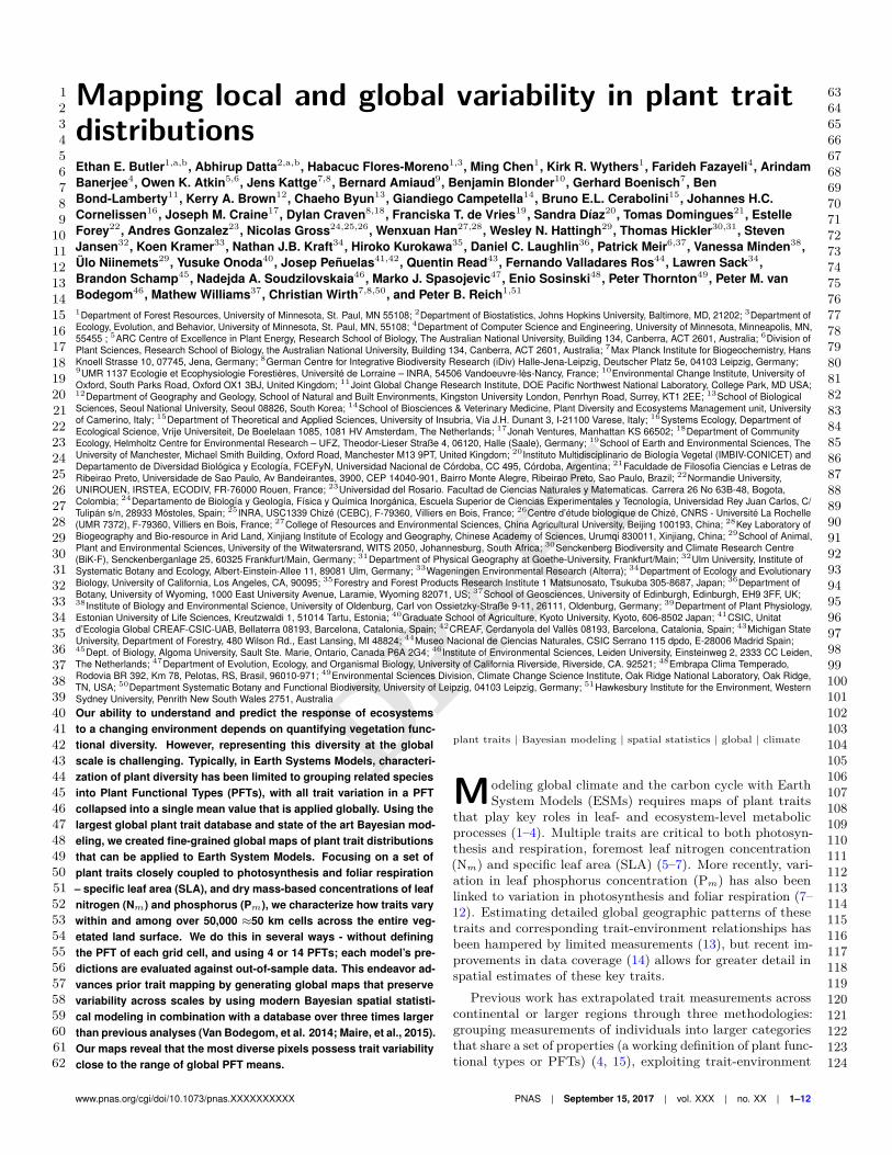
Mapping local and global variability in plant traitdistributionsEthan E. Butler1,a,b, Abhirup Datta2,a,b, Habacuc Flores-Moreno1,3, Ming Chen1, Kirk R. Wythers1, Farideh Fazayeli4, ArindamBanerjee4, Owen K. Atkin5,6, Jens Kattge7,8, Bernard Amiaud9, Benjamin Blonder10, Gerhard Boenisch7, BenBond-Lamberty11, Kerry A. Brown12, Chaeho Byun13, Giandiego Campetella14, Bruno E.L. Cerabolini15, Johannes H.C.Cornelissen16, Joseph M. Craine17, Dylan Craven8,18, Franciska T. de Vries19, Sandra Díaz20, Tomas Domingues21, EstelleForey22, Andres Gonzalez23, Nicolas Gross24,25,26, Wenxuan Han27,28, Wesley N. Hattingh29, Thomas Hickler30,31, StevenJansen32, Koen Kramer33, Nathan J.B. Kraft34, Hiroko Kurokawa35, Daniel C. Laughlin36, Patrick Meir6,37, Vanessa Minden38,Ülo Niinemets29, Yusuke Onoda40, Josep Peñuelas41,42, Quentin Read43, Fernando Valladares Ros44, Lawren Sack34,Brandon Schamp45, Nadejda A. Soudzilovskaia46, Marko J. Spasojevic47, Enio Sosinski48, Peter Thornton49, Peter M. vanBodegom46, Mathew Williams37, Christian Wirth7,8,50, and Peter B. Reich1,51
1Department of Forest Resources, University of Minnesota, St. Paul, MN 55108; 2Department of Biostatistics, Johns Hopkins University, Baltimore, MD, 21202; 3Department ofEcology, Evolution, and Behavior, University of Minnesota, St. Paul, MN, 55108; 4Department of Computer Science and Engineering, University of Minnesota, Minneapolis, MN,55455 ; 5ARC Centre of Excellence in Plant Energy, Research School of Biology, The Australian National University, Building 134, Canberra, ACT 2601, Australia; 6Division ofPlant Sciences, Research School of Biology, the Australian National University, Building 134, Canberra, ACT 2601, Australia; 7Max Planck Institute for Biogeochemistry, HansKnoell Strasse 10, 07745, Jena, Germany; 8German Centre for Integrative Biodiversity Research (iDiv) Halle-Jena-Leipzig, Deutscher Platz 5e, 04103 Leipzig, Germany;9UMR 1137 Ecologie et Ecophysiologie Forestières, Université de Lorraine – INRA, 54506 Vandoeuvre-lès-Nancy, France; 10Environmental Change Institute, University ofOxford, South Parks Road, Oxford OX1 3BJ, United Kingdom; 11Joint Global Change Research Institute, DOE Pacific Northwest National Laboratory, College Park, MD USA;12Department of Geography and Geology, School of Natural and Built Environments, Kingston University London, Penrhyn Road, Surrey, KT1 2EE; 13School of BiologicalSciences, Seoul National University, Seoul 08826, South Korea; 14School of Biosciences & Veterinary Medicine, Plant Diversity and Ecosystems Management unit, Universityof Camerino, Italy; 15Department of Theoretical and Applied Sciences, University of Insubria, Via J.H. Dunant 3, I-21100 Varese, Italy; 16Systems Ecology, Department ofEcological Science, Vrije Universiteit, De Boelelaan 1085, 1081 HV Amsterdam, The Netherlands; 17Jonah Ventures, Manhattan KS 66502; 18Department of CommunityEcology, Helmholtz Centre for Environmental Research – UFZ, Theodor-Lieser Straße 4, 06120, Halle (Saale), Germany; 19School of Earth and Environmental Sciences, TheUniversity of Manchester, Michael Smith Building, Oxford Road, Manchester M13 9PT, United Kingdom; 20Instituto Multidisciplinario de Biología Vegetal (IMBIV-CONICET) andDepartamento de Diversidad Biológica y Ecología, FCEFyN, Universidad Nacional de Córdoba, CC 495, Córdoba, Argentina; 21Faculdade de Filosofia Ciencias e Letras deRibeirao Preto, Universidade de Sao Paulo, Av Bandeirantes, 3900, CEP 14040-901, Bairro Monte Alegre, Ribeirao Preto, Sao Paulo, Brazil; 22Normandie University,UNIROUEN, IRSTEA, ECODIV, FR-76000 Rouen, France; 23Universidad del Rosario. Facultad de Ciencias Naturales y Matematicas. Carrera 26 No 63B-48, Bogota,Colombia; 24Departamento de Biología y Geología, Física y Química Inorgánica, Escuela Superior de Ciencias Experimentales y Tecnología, Universidad Rey Juan Carlos, C/Tulipán s/n, 28933 Móstoles, Spain; 25INRA, USC1339 Chizé (CEBC), F-79360, Villiers en Bois, France; 26Centre d’étude biologique de Chizé, CNRS - Université La Rochelle(UMR 7372), F-79360, Villiers en Bois, France; 27College of Resources and Environmental Sciences, China Agricultural University, Beijing 100193, China; 28Key Laboratory ofBiogeography and Bio-resource in Arid Land, Xinjiang Institute of Ecology and Geography, Chinese Academy of Sciences, Urumqi 830011, Xinjiang, China; 29School of Animal,Plant and Environmental Sciences, University of the Witwatersrand, WITS 2050, Johannesburg, South Africa; 30Senckenberg Biodiversity and Climate Research Centre(BiK-F), Senckenberganlage 25, 60325 Frankfurt/Main, Germany; 31Department of Physical Geography at Goethe-University, Frankfurt/Main; 32Ulm University, Institute ofSystematic Botany and Ecology, Albert-Einstein-Allee 11, 89081 Ulm, Germany; 33Wageningen Environmental Research (Alterra); 34Department of Ecology and EvolutionaryBiology, University of California, Los Angeles, CA, 90095; 35Forestry and Forest Products Research Institute 1 Matsunosato, Tsukuba 305-8687, Japan; 36Department ofBotany, University of Wyoming, 1000 East University Avenue, Laramie, Wyoming 82071, US; 37School of Geosciences, University of Edinburgh, Edinburgh, EH9 3FF, UK;38Institute of Biology and Environmental Science, University of Oldenburg, Carl von Ossietzky-Straße 9-11, 26111, Oldenburg, Germany; 39Department of Plant Physiology,Estonian University of Life Sciences, Kreutzwaldi 1, 51014 Tartu, Estonia; 40Graduate School of Agriculture, Kyoto University, Kyoto, 606-8502 Japan; 41CSIC, Unitatd’Ecologia Global CREAF-CSIC-UAB, Bellaterra 08193, Barcelona, Catalonia, Spain; 42CREAF, Cerdanyola del Vallès 08193, Barcelona, Catalonia, Spain; 43Michigan StateUniversity, Department of Forestry, 480 Wilson Rd., East Lansing, MI 48824; 44Museo Nacional de Ciencias Naturales, CSIC Serrano 115 dpdo, E-28006 Madrid Spain;45Dept. of Biology, Algoma University, Sault Ste. Marie, Ontario, Canada P6A 2G4; 46Institute of Environmental Sciences, Leiden University, Einsteinweg 2, 2333 CC Leiden,The Netherlands; 47Department of Evolution, Ecology, and Organismal Biology, University of California Riverside, Riverside, CA. 92521; 48Embrapa Clima Temperado,Rodovia BR 392, Km 78, Pelotas, RS, Brasil, 96010-971; 49Environmental Sciences Division, Climate Change Science Institute, Oak Ridge National Laboratory, Oak Ridge,TN, USA; 50Department Systematic Botany and Functional Biodiversity, University of Leipzig, 04103 Leipzig, Germany; 51Hawkesbury Institute for the Environment, WesternSydney University, Penrith New South Wales 2751, AustraliaOur ability to understand and predict the response of ecosystemsto a changing environment depends on quantifying vegetation func-tional diversity. However, representing this diversity at the globalscale is challenging. Typically, in Earth Systems Models, characteri-zation of plant diversity has been limited to grouping related speciesinto Plant Functional Types (PFTs), with all trait variation in a PFTcollapsed into a single mean value that is applied globally. Using thelargest global plant trait database and state of the art Bayesian mod-eling, we created fine-grained global maps of plant trait distributionsthat can be applied to Earth System Models. Focusing on a set ofplant traits closely coupled to photosynthesis and foliar respiration– specific leaf area (SLA), and dry mass-based concentrations of leafnitrogen (Nm) and phosphorus (Pm), we characterize how traits varywithin and among over 50,000 ≈50 km cells across the entire veg-etated land surface. We do this in several ways - without definingthe PFT of each grid cell, and using 4 or 14 PFTs; each model’s pre-dictions are evaluated against out-of-sample data. This endeavor ad-vances prior trait mapping by generating global maps that preservevariability across scales by using modern Bayesian spatial statisti-cal modeling in combination with a database over three times largerthan previous analyses (Van Bodegom, et al. 2014; Maire, et al., 2015).Our maps reveal that the most diverse pixels possess trait variabilityclose to the range of global PFT means.
plant traits | Bayesian modeling | spatial statistics | global | climate
Modeling global climate and the carbon cycle with EarthSystem Models (ESMs) requires maps of plant traits
that play key roles in leaf- and ecosystem-level metabolicprocesses (1–4). Multiple traits are critical to both photosyn-thesis and respiration, foremost leaf nitrogen concentration(Nm) and specific leaf area (SLA) (5–7). More recently, vari-ation in leaf phosphorus concentration (Pm) has also beenlinked to variation in photosynthesis and foliar respiration (7–12). Estimating detailed global geographic patterns of thesetraits and corresponding trait-environment relationships hasbeen hampered by limited measurements (13), but recent im-provements in data coverage (14) allows for greater detail inspatial estimates of these key traits.
Previous work has extrapolated trait measurements acrosscontinental or larger regions through three methodologies:grouping measurements of individuals into larger categoriesthat share a set of properties (a working definition of plant func-tional types or PFTs) (4, 15), exploiting trait-environment
www.pnas.org/cgi/doi/10.1073/pnas.XXXXXXXXXX
123456789
1011121314151617181920212223242526272829303132333435363738394041424344454647484950515253545556575859606162
63646566676869707172737475767778798081828384858687888990919293949596979899100101102103104105106107108109110111112113114115116117118119120121122123124
PNAS | September 15, 2017 | vol. XXX | no. XX | 1–12

DRAFT
relationships (e.g. leaf Nm and mean annual temperature)(1, 16–19), or restricting the analysis to species whose pres-ence has been widely estimated on the ground (20–23).Each of these methods has limitations - for example, trait-environment relationships do not well explain observed traitspatial patterns(1, 24), while species-based approaches limitthe scope of extrapolation to only areas with well measuredspecies abundance. More critically, the first two global method-ologies emphasized estimating a single trait value per PFTat every location, whereas both ground based (5, 14) and re-motely sensed (25) observations suggest that at ecosystem orlandscape scales traits would be better represented by distri-butions. Here, we use an updated version of the largest globaldatabase of plant traits (14) coupled with modern Bayesianspatial statistical modeling techniques (26) to capture localand global variability in plant traits. This combination allowsthe representation of trait variation both within pixels on agridded land surface as well as across global environmentalgradients.
Information is lost when the range of measured trait valuesis compressed into a single PFT (Fig. 1). We observe thatthe global range of site level SLA values for a single PFTsuch as Broadleaf Evergreen Tropical trees (Fig. 1a,c) is quitelarge (2.7 to 65.2 m2 kg−1). Even after limiting the scope toa single well measured 0.5◦ × 0.5◦ pixel within Panama (Fig.1b,c), there is still a wide range of SLA values (4.7 to 37.7 m2
kg−1) with a local mean of 15.7 m2 kg−1, and a local standarddeviation of 5.4 m2 kg−1 – over 1/3 of the local mean. Bycontrast, the mean SLA value of all species associated withBroadleaf Evergreen Tropical trees is 13.9 m2 kg−1, over 10%lower than the local average (Fig. 1c). Thus, single traitvalues per PFT fail to capture variability in trait values withinor among grid cells; i.e. over a wide range of spatial scales.
Transitioning from a single trait value per PFT to a distri-bution may lead to significantly different modeling results ascritical plant processes, such as photosynthesis, are non-linear
Significance Statement
Currently, Earth System Models (ESMs) represent variation inplant life through the presence of a small set of Plant Func-tional Types (PFTs), each of which accounts for hundreds orthousands of species across thousands of vegetated grid cellson land. By expanding plant traits from a single mean valueper PFT to a full distribution per PFT that varies among gridcells, the trait variation present in nature is restored and maybe propagated to estimates of ecosystem processes. Indeed,critical ecosystem processes tend to depend on the full trait dis-tribution, which therefore needs to be represented accurately.These maps re-introduce substantial local variation and willallow for a more accurate representation of the land surface inESMs.
The general idea for the study was developed by E.E.B., A.D, H.F.M., F.F., M.C., K.W., A.B., J.K.,O.K.A., and P.B.R.; specifics were developed by E.E.B. and A.D., and refined with the rest of thatteam. Data were made available by the hundreds of contributors to the TRY database; with furtherdata management and compilation by E.E.B, A.D., H.F.M. and J.K. E.E.B. and A.D. performed theanalysis, with all authors contributing to interpretation. E.E.B. and A.D. wrote the first draft; allauthors contributed to subsequent versions, including the submitted one.
The authors declare no known conflicts of interest.
aE.E.B and A.D. contributed equally to this work.
bTo whom correspondence should be addressed. E-mail: [email protected], [email protected]
with respect to these traits (27). This is reinforced by recentmodeling studies which have begun to incorporate distribu-tions of traits at regional (28, 29) and global (30) scales. Ithas been shown that using trait distributions leads to differ-ent estimates of carbon dynamics (31) and that higher ordermoments of trait distributions contribute to sustaining mul-tiple ecosystem functions (32). While species level mapping(20, 22, 23) does capture trait distributions, it has been limitedgeographically and restricted to subsets of functional groups.
Even the largest plant trait database offers only partialcoverage across the globe in terms of site level measurements.Hence, gap-filling approaches need to be adopted to extrapo-late trait values at regions with no data coverage. Here, weovercome data limitations through PFT classification, trait-environment relationships, and additional location informationto develop a suite of models capable of estimating trait dis-tributions across the entire vegetated globe. The simplest isa categorical model, which assigns traits to maps of remotelysensed PFTs. Every species, with its corresponding trait val-ues, is associated with a PFT and these trait distributionsare extrapolated to the satellite estimated range of the PFT(Figs. S1-S2). The second is a Bayesian linear model whichcomplements the PFT information with trait-environmentrelationships. The third is a Bayesian spatial model which,in addition to PFTs and the trait-environment relationships,leverages additional location information via Gaussian Pro-cesses (Methods). The use of a spatial Gaussian Process inthis context is novel and model evaluation reveals the superiorpredictive performance of this model.
Each of these methods interpolate (and extrapolate) bothmean trait values and entire trait distributions across space (i.e.across grid cells on a global map). These models are furtherstratified by three different levels of PFT categorization: 1)global, all plants in a single group; 2) broad, four groups basedon growth form and leaf type; 3) narrow, fourteen groups basedon further environmental, phenological, and photosyntheticcategories (Methods). The global categorization groups allplants into a single class, while the broad grouping (4-PFT)is similar to the vegetation classification used in the JULESland surface (33), and the narrow (14-PFT) categories areequivalent to the classification used in the Community LandModel (4, 15, 34).
The above mentioned methods allow for a representationof global vegetation that enables a more accurate formulationof functional diversity than the single trait value per PFTparadigm that is widely employed (4). The traits studied here- SLA, Nm, and Pm - are central to predicting variation inrates of plant photosynthesis (5, 6, 9, 11) and foliar respira-tion (10, 35). The importance of these traits and the moreadvanced representation of functional diversity developed heremay be used to better capture the response of the land surfacecomponent of the Earth System to environmental change.
Results and Discussion
Model Evaluation. Given the full suite of nine models proposed,we conducted extensive model evaluation (see Table 1) todetermine the trade-offs associated with each methodology andresolution of PFT. We assessed the predictive capability of themodels using the root mean squared predictive error (RMSPE)based on out-of-sample data (see Section S6). Among thenine models, the spatial narrow 14-PFT model emerged as
2 | www.pnas.org/cgi/doi/10.1073/pnas.XXXXXXXXXX
125126127128129130131132133134135136137138139140141142143144145146147148149150151152153154155156157158159160161162163164165166167168169170171172173174175176177178179180181182183184185186
187188189190191192193194195196197198199200201202203204205206207208209210211212213214215216217218219220221222223224225226227228229230231232233234235236237238239240241242243244245246247248
Butler and Datta et al.

DRAFT
the best predictor of mean trait values for SLA and Nm, andthe second best for Pm (Table 1). However, the spatial broad4-PFT model performed nearly as well (Table 1). The closepredictive skill of the broad PFT model and the narrow PFTmodel suggests that variations in growth form and leaf type,used to define the 4 broad PFTs, are more strongly related tovariations of trait values than bioclimatic differences, whichare used in the global spatial model. The models’ abilitiesto correctly estimate the spread of the trait distributionswere assessed using the out-of-sample coverage probabilities(CP) – the proportion of instances the model predicted 95%confidence intervals contained the observed trait values. Mostof the models provided adequate coverage (CP of around 90%or more). See Section S4 for more detailed definitions of themodel comparison metrics.
The improvement in prediction afforded by the inclusion ofa spatial term and PFT information invites further evaluation(Table 1). Spatial relationships play a substantial role inshaping trait values, at least at the global scale. The spatialterm in the model is likely to approximate finer scale variationthat is unavailable for the large grid cells of global analyses.For example, smaller scale studies that can evaluate localvariations in climate, soil, or other relevant abiotic or bioticcovariates are unlikely to see as much improvement with the useof a spatial term, as they may directly measure local sourcesof variability. However, with large grid cells the spatial termallows for local adjustment of trait values that the relativelycoarse environmental metrics are not able to capture. Similarly,the use of PFTs greatly improves the models. The greatestdecrease in RMSPE occurs between the global grouping (singleglobal PFT-equivalent) and the broad (4-PFT) grouping acrosseach of the models tested. This implies that the broad PFTs,based primarily on growth form and leaf type, offer superiorpredictive skill than environmental covariates on their own(19). However, the extra information in the narrow (14-PFT)grouping does further improve the fit and produces the mostaccurate predicted trait surface.
Global Maps. As the narrow 14-PFT spatial model is the bestpredictor of mean trait values, and provided adequate coverageprobability, we show the mean and standard deviation mapsfor this model (Fig. 2-4a,b). To provide a comparison, wealso included the best map closest to those currently employedin ESMs - the narrow PFT categorical model (Fig. 2-4c,d).Maps for the other models can be found in the supplementalmaterial (Figs. S8-S16). The mean and standard deviationare presented as a summary of the full log-normal distributionwithin each pixel, but there are full distributions estimated ineach pixel, see Case Studies below.
The standard deviation maps (Figs. 2-4b,d) compared tothe mean maps (Figs. 2-4a,c) highlight one of the centralresults of this analysis – the local standard deviations of traitvalues are of similar magnitudes as their respective means.Generally, we observed that the local standard deviation isclose to half the local mean value but can approach the globalrange of the trait mean values, e.g. Nm (Fig. 3) has a maxi-mum local standard deviation of 9 mg N / g, and the globalmean range is only ≈10 mg N / g. The maps of the trait stan-dard deviations follow similar patterns to the means, thoughthere are several regions where the mean varies more rapidlythan the standard deviation; such as SLA in the SE UnitedStates and China in the categorical model (Fig. 2c,d) and
similarly for Nm in the spatial model across the Sahel in sub-Saharan Africa (3a,c). The lack of variation in the standarddeviation is most clear in the categorical model for Nm whileboth models show relatively modest variation in Pm.
While the broad features of the mean maps for both thecategorical and spatial models are similar across SLA (Fig. 2),Nm (Fig. 3), and Pm (Fig. 4); there are numerous markeddifferences across both broad and fine spatial scales. Theshared broad features of the maps from both models includeSLA and Pm increasing from the tropics to the poles, whileNm has more modest variation, except that it tends to belower in regions dominated by needle-leaved trees. Some ofthe notable differences between the models include the spatialmodel’s greater range and more marked variability of SLAwithin equatorial regimes (e.g., Brazil or central Africa); italso better captures the low SLA of most of arid Australiathan the categorical model; and more strongly highlights thegradient of Pm from the tropics to the arctic (16) (Fig 2a,4a).
The most consistent estimates between the categorical andspatial models are in the boreal regions dominated by needle-leaf trees; the measurements in this region are relatively sparsewhich may have limited the ability of the spatial model tocapture differences. On the other hand, broad-leaved treesspan a wide range of environments, but a large portion of themeasurements come from the tropics (66%), where there isa limited range of values among the climate covariates andtherefore little variation with which to estimate a correlation.The grasses and shrubs have the largest standard deviationsof the four broad PFTs (Table S4) and dominate wide swathesof the land surface, but have fewer measurements – shrubs arethe least measured of the broad PFTs in the database, andthis appears to reduce the accuracy of the categorical modelmore than the spatial model (Table 1). The fact that shrubsare assumed to dominate in arid and boreal environments,which also tend to be under-sampled, also likely contributesto these differences.
Our results suggest that the breadth of functional nichespace is reduced in both boreal and tropical biogeographicregions. The low variation across all three traits within theboreal forest implies that there is strong filtering and smallerniche space available in this relatively harsh environment. Sur-prisingly, despite the high species diversity in tropical forests,we also find that SLA and Pm have relatively low variation inthese forests – suggesting that in this environment the traitspace is reduced. This could be, in part, an artifact of theEarth System Model PFT classification omitting herbaceousspecies. Conversely, grasslands and savannahs exhibit largevariation in total trait space, suggesting these environmentspermit a wider range of strategies than in both the borealand tropical regions. Most broadly, both the data and thespatial model indicate (Figs. S24,S25) low leaf nitrogen val-ues in temperate climates that increase in both colder andwarmer regions; this may indicate a more complicated leafbiochemistry-temperature relationship than has previouslybeen suggested (16).
Case Studies. As a more detailed evaluation of the true andpredicted shape of the trait distributions cannot be obtainedfrom the coverage probability or standard deviation maps,we conducted two regional case studies, in which trait datawere pooled over an area to construct full trait distributionsand these were formally compared with the model predicted
Butler and Datta et al.
249250251252253254255256257258259260261262263264265266267268269270271272273274275276277278279280281282283284285286287288289290291292293294295296297298299300301302303304305306307308309310
311312313314315316317318319320321322323324325326327328329330331332333334335336337338339340341342343344345346347348349350351352353354355356357358359360361362363364365366367368369370371372
PNAS | September 15, 2017 | vol. XXX | no. XX | 3

DRAFT
distributions.We considered two areas with substantially different envi-
ronmental conditions to evaluate the trait distributions ob-tained from the spatial and categorical models. We chose asingle pixel that contained a highly studied site with numerousmeasurements of tropical trees, Barro Colorado Island (BCI),Panama, and a collection of pixels in an arid environment inwhich the mean estimates for SLA of the spatial and categori-cal models substantially disagreed, the southwestern UnitedStates. These areas were in the training data, and this analysisconstituted a more detailed analysis of the models’ fit to theobserved distribution of these locations. Here, the focus wason the structure of the full distribution of traits predictedat these sites; Fig. S17 is a map of the measurements thatcomprised these locations and other sites included in this anal-ysis. Both areas offer further insight into the structure of thedistributions estimated by the categorical and spatial models.
In the pixel containing BCI, the categorical and spatialmodels broadly agreed for all three traits (Fig. 5a, c, e),although the spatial model means were only half as distantfrom the observed means for SLA and Nm (4% vs. 8% and5% vs. 10%, respectively). There were only two PFTs presentin this pixel: tropical broadleaf evergreen and deciduous trees.Despite the general similarity of the shapes of the distribution,the spatial model appears capable of capturing some subtlefeatures. This is clearest for leaf nitrogen, where the peak ofthe distribution was quite broad. This is neatly captured in thenarrow PFT model, and the pattern was detectable throughthe Kolmogorov-Smirnov (K-S) statistic, which evaluates thesimilarity of two full distributions. Indeed, the superiority ofthe spatial model was reinforced by a closer match for theBayesian spatial model across all traits at BCI (Table S6),though for Pm it was the global spatial model that fit best(not shown in the figure).
The differences between the trait distributions of the cate-gorical and Bayesian spatial models were stark in the south-western United States, although the mean estimates for Nm
and Pm were close (Fig. 5b, d, f). This may be a result ofthe topographic complexity of this region and the resultingdifficulty of aggregating climate and soil covariates at the0.5◦ pixel scale and the sparser sampling than at BCI. Toget enough data to approximate a distribution, we aggregated18 pixels with nine PFTs including every temperate category,though many of them are only marginally present. The inclu-sion of so many PFTs produced a noisier distribution in thecategorical model than suggested by the data and estimatedby the spatial model. Neither of the models produced distribu-tions that matched as well with the observations; however, itis notable how close the mean values for both models matchedthe observations for Nm and Pm, and the spatial model didwell for the mean SLA.
Environmental Covariates and the Spatial Term. The improve-ment in prediction from the linear model to the spatial modelwas partially explained by the weak trait-environment rela-tionships presented in Tables S2-S4. The magnitude of thespatial variation explained with the Gaussian process modelwas of similar magnitude as the unexplained trait variation.For most of the spatial models, the estimated spatial rangewas around 500 kilometers; this suggests a strong spatial effect,and implies that the spatial model can provide more preciseinformation about the trait distribution near the locations
where we have data. This was largely borne out in the casestudies, and is illustrated more explicitly in Fig. 6 where thepredicted trait standard deviation for the spatial model was upto 50% lower than the linear non-spatial model near locationswith trait measurements. The spatial model thus leverageslocal information to reduce the uncertainty of trait estimationnear data locations and may provide guidance for future datacollection by identifying high uncertainty regions.
Applications for Trait Distributions. Plant traits vary across arange of spatial scales, and the spatial model best captures thelarge spatial gradients (such as in Amazonia and Australia) aswell as the subtleties within pixels. Maps for all the modelshighlight how much information about local variability is lostwhen representing plant traits with a single value, and suggeststhat a first application of these maps will be for ESMs toincorporate these scales of variability. For process-based ESMs,the simplest model to incorporate will likely be the categoricalmodel as it is closest to the current PFT approach, but thismodel is also the least flexible. The more sophisticated modelsdeveloped here provide more accurate large scale variation,and may be used to infer new trait values in a novel climateby perturbing the climatic covariates (36). However, given thelikelihood of non-linear trait-environment relationships, thespatial sparsity of the data, and the possibility of alternatestrategies within a PFT that may alter the trait-environmentrelationship in a future climate some caution is called for whenusing these models for extrapolation.
We have emphasized the quality of the Bayesian spatialmodel with narrow PFTs, but there is an intriguing possibilityopened by the global model (Fig. S8, S11, and S14) – thatbeing the representation of vegetation without reference toPFTs (1). In this case the representation of vegetation wouldrely entirely on the structure of trait distributions at variouslandscape scales (1). Such a representation eliminates the needto separately model the future locations of PFTs (or species)when inferring the future distribution of traits; hence, theoutput of a model like that developed here could be updatedwith future environmental covariates, with the caveats that‘out of sample prediction’ may entail. At the same time,this method would allow for greater functional diversity thanmultiple PFTs with single trait values, as is currently used inmost ESMs. Adopting this approach does, however, raise theissue of how to deal with the paucity of surface observationsin some regions, as evidenced by the greater errors associatedwith estimating out of sample values with this model (Table1). Complementary work has retrieved leaf trait maps froma global carbon cycle model fused with Earth observations(37), providing another method that could be used for directcomparison against the trait maps produced here. While themethodology outlined in our analysis brings the possibility of aPFT-free land surface closer, the current level of observationsremains insufficient to provide superior prediction of traitvalues for all surface regions; given this, there is a necessity tocontinue use of PFTs for trait prediction until the paucity oftrait data is rectified.
Conclusions
SLA and Nm are essential inputs into the land surface compo-nents of Earth System Models, and while phosphorus has notyet been as widely incorporated into ESMs, it has been shown
4 | www.pnas.org/cgi/doi/10.1073/pnas.XXXXXXXXXX
373374375376377378379380381382383384385386387388389390391392393394395396397398399400401402403404405406407408409410411412413414415416417418419420421422423424425426427428429430431432433434
435436437438439440441442443444445446447448449450451452453454455456457458459460461462463464465466467468469470471472473474475476477478479480481482483484485486487488489490491492493494495496
Butler and Datta et al.

DRAFT
- particularly across the tropics - to be important to photosyn-thesis (9, 11, 38–41) and respiration (11, 12, 35). The mapsand trait-environment relationships presented here may beused by existing land surface models that use similar categoriesto classify vegetation. However, it should be noted that PFT-dependent models often have many other parameters that havebeen calibrated to historical estimates of particular trait values(4). Thus, the values developed here, while likely drawing froma larger pool of measurements than has been done previouslycan not necessarily be adopted without further modificationof other model elements (36, 42). Nonetheless, these resultscan be incorporated into a wide class of models with relativeease. We can now provide global trait distributions at thepixel scale.
The global land surface is perhaps the most heterogeneouscomponent of the Earth System. Reducing vegetation to a col-lection of PFTs with fixed trait values has been the preferredmethod to constrain this heterogeneity and group similar bio-chemical and biophysical properties; however, this has been atthe expense of functional diversity. This analysis quantifies thesubstantial magnitude of this ignored trait variation. The ap-proach and methods presented here retain the simplicity of thePFT representation, but capture a wider range of functionaldiversity.
Materials and Methods
Data. The TRY database (www.try-db.org) (14) provided alldata for leaf traits and the categorical traits to aggregatePFTs (TRY – Categorical Traits Dataset, https://www.try-db.org/TryWeb/Data.php#3, January 2016) used in the analysis.See Appendix 1 for a complete list of the original publications asso-ciated with this subset of TRY. The extract from TRY used here hasjust under 45,000 measurements of individuals from 3,680 specieswith measurements of at least one of specific leaf area (SLA), leafnitrogen per dry leaf mass (Nm), and/or leaf phosphorus per leafdry mass (Pm). The number of individual measurements varies from32,315 for SLA on 2,953 species to 19,282 for Nm on 3,053 speciesdown to 8,052 for Pm on 1,810 species; see Table S4 for the numberof unique measurements and species found in all categorizationsused in the analysis. The species taxonomy was standardized usingThe Plant List (43). Measurements were associated with environ-mental categories through Köppen-Geiger climate zones (44). Allenvironmental variables are on a 0.5◦ × 0.5◦ grid. Climate vari-ables use 30 year climatologies from 1961-1990 as estimated by theClimate Research Unit (45, 46). Soil variables are from the Interna-tional Soil Reference and Information Center - World Inventory ofSoil Emission Potentials (ISRIC-WISE) (47). The spatial extent ofPFTs have been previously estimated through satellite estimatesof land cover around the year 2005 (48), and these estimates havebeen refined into climatic categories (15, 34). While TRY, and thusthe data used here, represents the largest collection of plant traitsin the world most of the measurements come from a subset of globalregions: North America, Europe, Australia, China, Japan, andBrazil. There are still large sections of the planet with extremelysparse measurements, notably: much of the tropics outside of theAmericas, large swathes of Central Asia, the Russian Federation,South Asia and much of the Arctic (fig. S17). Improving datacollection in these regions will greatly improve future modelingefforts.
Classification of PFTs and Categorical Model. We used three nestedlevels of PFT classification. In the first level, all plants are cate-gorized into a single global group (‘global’). In the second level(‘broad’), all plants are categorized into PFTs based on categor-ical traits associated with growth form (grass, shrub, tree) andleaf type (broad and needle-leaved) leading to the following fourPFTs: grasses, shrubs, broad-leaved trees and needle-leaved trees
(Fig. S1). In the third level (‘narrow’), the broad PFTs are furtherrefined by their climatic region – tropical, temperate, boreal – aswell as leaf phenology, and, for the grasses, photosynthetic pathway(C3 or C4). This produces 14 PFTs (Fig. S2), which correspondexactly to those found in the community land model (CLM) (4).Note that these PFT classifications exclude non-woody eudicots(‘herbs’), which were excluded from the analysis, on account of theirlack of dominance within these PFT categories (49) and therefore,on account of being widely measured could overly influence thestructure of the trait distributions if they were included. Satelliteestimates of the PFT abundance that correspond to the “narrow”PFT categories defined above have already been calculated (15, 48)and we used these to assign a percentage of each 0.5◦ × 0.5◦ pixelto each PFT present according to the fraction of the land surfacewithin that pixel occupied by the PFT. The “broad” PFT fractionsare calculated by summing the narrow PFT categories within each“broad” classification.
The categorical model uses the PFT categories and averagestrait values for each species across individual measurements at eachmeasured location. This defines the PFT as the interspecies rangeof trait values and ignores all local environmental factors. Theresults of the categorical model are summarized by the mean andstandard deviation of each PFTs trait values (Table S4) for all threeresolutions of the model. Note that in the global case where noPFT information is used, the categorical model produces a constanttrait distribution across the entire vegetated world. The categoricalmodel, and the Bayesian models described in the following sectionall use location specific species mean values to estimate trait dis-tributions. We assume no intra-specific variation in trait values.However, in regions dominated by a small number of species thismay lead to biased predictions. The hyper dominance of a smallgroup of species in the Amazon has recently been demonstrated(50) and thus serves as a case study to evaluate our assumption ofequal species weighting (S8, fig. S23). We found that equal weights(species means) produced trait distribution estimates closest tothose of the hyper dominant trait abundances and this reinforcesthe use of this assumption globally. Further, as noted above, theomission of herbaceous species from tropical regions in this analysis(and (50)) may unduly limit trait diversity, and calls for furtherresearch.
Bayesian Models. A more fine-tuned depiction of geographical or spa-tial variation of plant trait values within each PFT can be achievedby leveraging environmental and location information, which allowstrait values to adjust based on local conditions. Data for 17 climate(45, 46) and soil based (47) environmental predictors were availableat the 0.5◦ × 0.5◦ pixel resolution used to create the trait maps. Toavoid overfitting and collinearity issues, these seventeen predictorswere screened (see Section S7) based on correlations amongst pre-dictors, their individual correlation with the traits, and to includeclimate covariates along different axes of environmental stress andboth chemical and physical soil covariates. We finally selected fivepredictors – mean annual temperature [MAT], total annual radia-tion [RAD], moisture index (precipitation/evapotranspiration) [MI],percent hydrogen (aqueous) [pH], and percent clay content [CLY].Remote sensing data products, such as Normalized Difference Vege-tation Index (51)), are not used as covariates, to allow for inferenceoutside of the historical observation period through perturbationsof environmental covariates.
We utilized environment-trait relationships to obtain predictionsof trait values (1, 16–18, 36, 42) in a linear regression setup. Theformal details of the initial model are as follows. We denote log-transformed trait values at a geographical location s as ytrait(s).This set of five predictors at a location s is denoted by the vectorx(s) = (x1(s), x2(s), ..., x5(s))′. A linear regression model relatingthe trait to the environmental predictors is specified as:
ytrait(s) = b0 + b1x1(s) + b2x2(s) + ...+ b5x5(s) + ε(s) [1]
where bi are the regression coefficients and ε(s) is the error termexplaining residual variation. Estimation of model parameters andprediction were achieved with a fully Bayesian hierarchical model.This enables inclusion of prior information and prediction of full traitdistributions instead of representative values (like mean or median)thereby ensuring that the uncertainty associated with the estimation
Butler and Datta et al.
497498499500501502503504505506507508509510511512513514515516517518519520521522523524525526527528529530531532533534535536537538539540541542543544545546547548549550551552553554555556557558
559560561562563564565566567568569570571572573574575576577578579580581582583584585586587588589590591592593594595596597598599600601602603604605606607608609610611612613614615616617618619620
PNAS | September 15, 2017 | vol. XXX | no. XX | 5

DRAFT
of model parameters is fully propagated into the predictive traitdistributions.
We then generalized the above model into a Bayesian spatial lin-ear regression model that borrows information from geographicallyproximal regions to capture residual spatial patterns beyond whatis explained by environmental predictors. A customary specificationof a spatial regression model is obtained by splitting up the errorterm ε(s) in Equation (1) into the sum of a spatial process w(s)and an error term η(s), that accounts for the residual variationafter adjusting for the spatial effects w(s). The underlying latentprocess w(s) accounts for local nuances beyond what is capturedby the environmental predictors and is often interpreted as the netcontribution from unobserved or unusable predictors. Gaussian Pro-cesses (GP) are widely used for modeling unknown spatial surfacessuch as w(s), due to their convenient formulation as a multivariateGaussian prior for the spatial random effect, unparalleled predic-tive performance (52) and ease of generating uncertainty quantifiedpredictions at unobserved locations. We use the computationallyeffective Nearest Neighbor Gaussian Process (26) which nicely em-beds into the Bayesian hierarchical setup as a prior for w(s) in thesecond stage of the model specification. All technical specificationsof the Bayesian spatial model are provided in Section S1 of thesupplementary materials.
The linear regression models used in previous studies (1, 16–18)and both the spatial and non-spatial Bayesian models describedabove assume a global relationship between the traits and environ-ment. Given the goal of predicting trait values for the entire landsurface, the assumption of a universal trait-environment relationshipmay be an oversimplification (53). Moreover, if there is significantvariation in plant trait values among different PFTs, the estimatedparameters will be skewed towards values from abundantly sampledPFTs, such as broad-leaved trees. Additional information aboutplant characteristics at a specific location, if available, can poten-tially be used to improve predictions. As mentioned earlier, we havePFT classifications for each observation of the dataset used hereand satellite estimates of PFT abundance at all pixels. The globalregression approaches described above ignores this information andcan yield biased predictions at locations dominated by PFTs poorlyrepresented in the data, such as shrubs. Hence, we also incorpo-rate the PFT information in these regression models by allowingthe trait-environment relationship to vary between different PFTs.Finally, the PFT specific distributions from the Bayesian modelswere weighted by the satellite based PFT abundances to create alandscape scale trait distribution, thereby enabling straightforwardcomparison between all three categorizations of PFT. Details of thePFT based Bayesian models are provided in Section S2. The useof a Gaussian Process based spatial model as well as the Bayesianimplementation of the regression models were novel to this applica-tion of plant trait mapping and, as results indicated, were criticalto improving model predictions as well as properly quantifying traitdistributions.
All the code and public data are available from the authors uponrequest. The TRY data may be requested from the TRY databasecustodians.
ACKNOWLEDGMENTS. E.E.B., H.F.M., M.C., K.R.W., andP.B.R. acknowledge funding from the United States Department ofEnergy, Office of Science (DE-SC0012677). O.K.A. acknowledgesthe support of the Australian Research Council (CE140100008).P.B.R also acknowledges support from two University of MinnesotaInstitute on the Environment Discovery Grants. The study has beensupported by the TRY initiative on plant traits (http://www.try-db.org). The TRY initiative and database is hosted, developed andmaintained at the Max Planck Institute for Biogeochemistry, Jena,Germany. TRY is currently supported by DIVERSITAS/FutureEarth and the German Centre for Integrative Biodiversity Research(iDiv) Halle-Jena-Leipzig. BB acknowledges a NERC independentresearch fellowship NE/M019160/1. JP would like to acknowledgethe financial support from the European Research Council Synergygrant ERC-SyG-2013-610028 IMBALANCE-P, the Spanish Govern-ment grant CGL2013-48074-P and the Catalan Government grantSGR 2014-274. B.B.-L. was supported by the Earth System Model-ing program of the U.S. Department of Energy, Office of Science,Office of Biological and Environmental Research. KK acknowledges
the contribution of the WUR Investment theme Resilience for theproject Resilient Forest (KB-29-009-003). PM acknowledges supportfrom ARC grant FT110100457 and NERC NE/F002149/1. WHacknowledges support from the National Natural Science Founda-tion of China (#41473068) and “Light of West China” Program ofChinese Academy of Sciences.
1. Van Bodegom PM, Douma JC, Verheijen LM (2014) A fully traits-based approach to modelingglobal vegetation distribution. Proceedings of the National Academy of Sciences of the UnitedStates of America 111(38):13733–8.
2. Maire V, et al. (2015) Global effects of soil and climate on leaf photosynthetic traits and rates.Global Ecology and Biogeography 24(6):706–717.
3. DeFries RS, et al. (1995) Mapping the land surface for global atmosphere-biosphere models:Toward continuous distributions of vegetation’s functional properties. Journal of GeophysicalResearch 100(D10):20867.
4. Bonan GB, et al. (2011) Improving canopy processes in the Community Land Model version4 (CLM4) using global flux fields empirically inferred from FLUXNET data. Journal of Geo-physical Research 116(G2):1–22.
5. Reich PB, Ellsworth DS, Walters MB (1998) Leaf structure ( specific leaf area ) modulatesphotosynthesis – nitrogen relations : evidence from within and across species and functionalgroups. Functional Ecology 12:948–958.
6. Kattge J, Knorr W, Raddatz T, Wirth C (2009) Quantifying photosynthetic capacity and itsrelationship to leaf nitrogen content for global-scale terrestrial biosphere models. GlobalChange Biology 15(4):976–991.
7. Crous KY, et al. (2017) Nitrogen and phosphorus availabilities interact to modulate leaf traitscaling relationships across six plant functional types in a controlled-environment study. NewPhytologist.
8. Wright IJ, et al. (2004) The worldwide leaf economics spectrum. Nature 428(6985):821–827.9. Reich PB, Oleksyn J, Wright IJ (2009) Leaf phosphorus influences the photosynthesis-
nitrogen relation: A cross-biome analysis of 314 species. Oecologia 160(2):207–212.10. Atkin OK, et al. (2015) Global variability in leaf respiration in relation to climate, plant func-
tional types and leaf traits. New Phytologist 206(2):614–636.11. Bahar N, et al. (2016) Leaf-level photosynthetic capacity in lowland Amazonian and high
elevation, Andean tropical moist forests of Peru. New Phytologist.12. Rowland L, et al. (2016) Scaling leaf respiration with nitrogen and phosphorus in tropical
forests across two continents.13. Reich PB (2005) Global biogeography of plant chemistry: Filling in the blanks. New Phytolo-
gist 168(2):263–266.14. Kattge J, et al. (2011) TRY - a global database of plant traits. Global Change Biology
17(9):2905–2935.15. Oleson KW, et al. (2013) Technical Description of version 4.5 of the Community Land Model
(CLM), Technical Report Climate and Global Dynamics Division.16. Reich PB, Oleksyn J (2004) Global patterns of plant leaf N and P in relation to temperature
and latitude. Proceedings of National Academy of Sciences 101(30):11001–11006.17. Ordoñez JC, et al. (2009) A global study of relationships between leaf traits, climate and soil
measures of nutrient fertility. Global Ecology and Biogeography 18(2):137–149.18. Simpson AH, Richardson SJ, Laughlin DC (2016) Soil-climate interactions explain variation
in foliar, stem, root and reproductive traits across temperate forests. Global Ecology andBiogeography 25(8):964–978.
19. Reich PB, Wright IJ, Lusk CH (2007) Predicting Leaf Physiology from Simple Plant and Cli-mate Attributes : A Global GLOPNET Analysis. Ecological Applications 17(7):1982–1988.
20. Swenson NG, et al. (2012) The biogeography and filtering of woody plant functional diversityin North and South America. Global Ecology and Biogeography 21(8):798–808.
21. Hawkins BA, Rueda M, Rangel TF, Field R, Diniz-Filho JAF (2014) Community phylogeneticsat the biogeographical scale: Cold tolerance, niche conservatism and the structure of NorthAmerican forests. Journal of Biogeography 41(1):23–38.
22. Šímová I, et al. (2015) Shifts in trait means and variances in North American tree assem-blages: Species richness patterns are loosely related to the functional space. Ecography38(7):649–658.
23. Swenson NG, et al. (2017) Phylogeny and the prediction of tree functional diversity acrossnovel continental settings. Global Ecology and Biogeography pp. 1–12.
24. Douma JC, de Haan MWA, Aerts R, Witte JPM, van Bodegom PM (2012) Succession-induced trait shifts across a wide range of NW European ecosystems are driven by lightand modulated by initial abiotic conditions. Journal of Ecology 100(2):366–380.
25. Asner GP, Knapp DE, Anderson CB, Martin RE, Vaughn N (2016) Large-scale climatic andgeophysical controls on the leaf economics spectrum. Proceedings of National Academy ofSciences.
26. Datta A, Banerjee S, Finley A, Gelfand A (2016) Hierarchical Nearest-Neighbor GaussianProcess Models for Large Geostatistical Datasets. Journal of the American Statistical Asso-ciation 111(514):800–812.
27. Farquhar GD, von Caemmerer S, Berry JA (1980) A biochemical model of photosyntheticCO2 assimilation in leaves of C3 species. Planta 149(1):78–90.
28. Scheiter S, Higgins SI (2009) Impacts of climate change on the vegetation of Africa: Anadaptive dynamic vegetation modelling approach. Global Change Biology 15(9):2224–2246.
29. Scheiter S, Langan L, Higgins SI (2013) Next-generation dynamic global vegetation models:learning from community ecology. The New phytologist 198(3):957–69.
30. Pavlick R, Drewry DT, Bohn K, Reu B, Kleidon a (2012) The Jena Diversity-Dynamic GlobalVegetation Model (JeDi-DGVM): a diverse approach to representing terrestrial biogeogra-phy and biogeochemistry based on plant functional trade-offs. Biogeosciences Discussions9(4):4627–4726.
31. Pappas C, Fatichi S, Burlando P (2014) Terrestrial water and carbon fluxes across climaticgradients: does plant diversity matter? New Phytologist 16(i):3663.
32. Gross N, et al. (2017) Functional trait diversity maximizes ecosystem multifunctionality. Na-ture Ecology & Evolution 1(5):0132.
6 | www.pnas.org/cgi/doi/10.1073/pnas.XXXXXXXXXX
621622623624625626627628629630631632633634635636637638639640641642643644645646647648649650651652653654655656657658659660661662663664665666667668669670671672673674675676677678679680681682
683684685686687688689690691692693694695696697698699700701702703704705706707708709710711712713714715716717718719720721722723724725726727728729730731732733734735736737738739740741742743744
Butler and Datta et al.

DRAFT
33. Clark DB, et al. (2011) The Joint UK Land Environment Simulator (JULES), model description– Part 2: Carbon fluxes and vegetation dynamics. Geoscientific Model Development 4(3):701–722.
34. Bonan GB (2002) Landscapes as patches of plant functional types: An integrating conceptfor climate and ecosystem models. Global Biogeochemical Cycles 16(2):5.1–5.18.
35. Meir P, Grace J, Miranda AC (2001) Leaf respiration in two tropical rainforests: Constraintson physiology by phosphorus, nitrogen and temperature. Functional Ecology 15(3):378–387.
36. Verheijen LM, et al. (2015) Inclusion of ecologically based trait variation in plant functionaltypes reduces the projected land carbon sink in an earth system model. Global ChangeBiology 21(8):3074–3086.
37. Bloom AA, Exbrayat JF, van der Velde IR, Feng L, Williams M (2016) The decadal state of theterrestrial carbon cycle: Global retrievals of terrestrial carbon allocation, pools, and residencetimes. Proceedings of the National Academy of Sciences (22):1–6.
38. Meir P, Levy PE, Grace J, Jarvis PG (2007) Photosynthetic parameters from two contrastingwoody vegetation types in West Africa. Plant Ecology 192(2):277–287.
39. Domingues TF, et al. (2010) Co-limitation of photosynthetic capacity by nitrogen and phos-phorus in West Africa woodlands. Plant, Cell & Environment 33(6):959–980.
40. Zhang Q, Wang YP, Pitman AJ, Dai YJ (2011) Limitations of nitrogen and phosphorous onthe terrestrial carbon uptake in the 20th century. Geophysical Research Letters 38(22):1–5.
41. Medlyn B, et al. (2016) Using models to guide experiments: a priori predictions for the CO2response of a nutrient- and water-limited mature Eucalypt woodland. Global Change Biologypp. 2834–2851.
42. Verheijen LM, et al. (2013) Impacts of trait variation through observed trait-climate relation-ships on performance of an Earth system model: A conceptual analysis. Biogeosciences10(8):5497–5515.
43. 1.1 TPLV (2013) January. http://www.theplantlist.org/.44. Peel B, Finlayson BL, McMahon Ta (2007) Updated world map of the Köppen-Geiger climate
classification.pdf. Hydrology and Earth System Sciences 11:1633–1644.45. New M, Hulme M, Jones P (1999) Representing Twentieth-Century Space – Time Climate
Variability . Part I : Development of a 1961 – 90 Mean Monthly Terrestrial Climatology. Journalof Climate 12:829–856.
46. Harris I, Jones PD, Osborn TJ, Lister DH (2014) Updated high-resolution grids of monthlyclimatic observations - the CRU TS3.10 Dataset. International Journal of Climatology34(3):623–642.
47. Batjes N (2005) ISRIC-WISE: Global data set of derived soil properties on a 0.5 by 0.5 degreegrid (Version 3.0). (December):1–64.
48. Lawrence PJ, Chase TN (2007) Representing a new MODIS consistent land surface in theCommunity Land Model (CLM 3.0). Journal of Geophysical Research: Biogeosciences112(1).
49. Gibson DJ (2009) Grasses & Grassland Ecology. (Oxford University Press, New York).50. ter Steege H, et al. (2013) Hyperdominance in the Amazonian tree flora. Science
342(6156):1243092.51. Ollinger SV, et al. (2008) Canopy nitrogen, carbon assimilation, and albedo in temperate
and boreal forests: Functional relations and potential climate feedbacks. Proceedings of theNational Academy of Sciences of the United States of America 105(49):19336–41.
52. Rasmussen C (1996) Evaluation of Gaussian Processes and other methods for non-linearregression. (University of Toronto), Phd thesis edition.
53. Verheijen LM, Aerts R, Bönisch G, Kattge J, Van Bodegom PM (2016) Variation in trait trade-offs allows differentiation among predefined plant functional types: Implications for predictiveecology. New Phytologist 209(2):563–575.
Butler and Datta et al.
745746747748749750751752753754755756757758759760761762763764765766767768769770771772773774775776777778779780781782783784785786787788789790791792793794795796797798799800801802803804805806
807808809810811812813814815816817818819820821822823824825826827828829830831832833834835836837838839840841842843844845846847848849850851852853854855856857858859860861862863864865866867868
PNAS | September 15, 2017 | vol. XXX | no. XX | 7

DRAFT●
●
●
●
●
●
●
●
●
●●
●●●●
●
●●
●●●
●●
●
●
●
●
●●
●●●●●
●
●
●●●
●●●●
●●●●●
●
●●●●●
●●●●
●
●●●●
●
●●●●●●●●●●●●●
●
●●●●●●●●●●●●●
●●●●●●●
●●●●●●●●●●●●●●●●●●●●●●●●●●●●●●●●●●●●● ●
●●●●●●●●●
●●
●●
●
●●●●●●●●●
●
●●●● ●
●
●●●●●●●●●●●●●●●●●●●●●●●●●●●●●●●●●●●●●●●●●●●●●
●●●●●●●●●
●●●
●●●●●● ●●●●●●●●●●
7
8
9
10
−82 −80 −78Longitude
Latitude
0
20
40
60
SLA[m2 kg−1]
●●●
●
●
●
●
●
●
●
●
●
●
●●
●●●
●
●
●
●
●
●
●
●
●
●●
●
●
●
●
●
●
● ●
●
●
●
●●
●
●●
●
●●
●
●
●
●
●
●
●●
●
●
●
●
●
●
●
●
●
●●
●●
●
●
●●
●
●
●
●
● ●
●
●
●
●
●
●
●
●●
●●●
●
●
●
●
●
●
●
●
●
●●
●
●●
●●
●
●
●●
●
●
●
●
●
●
●
●●
●
●
●
●
●
●●
●
●
●
●
●
●
●
●
●
●
●
●
●
●
●
●●●
●
●
●●
●●
●
●
●
●
●●●●● ●●
●
●●
●
●
●
●●● ●●●●●
●
●
●
●
●
●
●
●
●
●
●
●
●
●
●
●
●
●
●
●
●
●
●●
●
●
●
●
●
●●
●
●
●
●
●
●
●
●●● ●
●
●
●
●
●
●●
●
● ●●●
●
●
●●
●
●
●● ●●
● ●●●
●
●
●
●
●
●
●
●
●
●
●
●
●
●
●
●●
●
●●●●
●
●
●
●
●●● ●●
●
●
●●●
●
●● ●
●
●
●
●
●
●
●
●
●
●
● ●
●
●
●
●
●
●
●
●
●
●
●
●
●
●
●
●
●
●●●●
●
●
●
●
●
●
●●●
●
●●●
●
●
●●
●
●
●
●●
●
●
●
●
●
●
●
●
●●
●●
●●●●●
●
●
●
●
●●
●●
●
●●
●
●
●
●
● ●
●
●
●
●
●
●
●
●
●●
●●● ●
●●●
●
●●●
●
●
●
●●
●●
●
●
●●
●
●
●
●
●
●●
●
●
● ●
●
●●
●
●
●●●
●
●
●●
●
●●
●
●●
●
●
●
●
●●
●
● ●
●●
●
●
●
●
●
●●
●
●
●
●
●
●
●
●
●
●
●
●●●
●
●
●●
●
●
●
●●
●
●
●
●
●●●
●
●
●
●●
●
●
●●
●
●
●●
● ●
●
●●
●
●
● ●
●
●●
●
●
●●
●
●
●
●
●●
●
●●●
●
●●●
●
●
●●
●
●
●
●
●
●
●
●
●
●
●
●
●
●●
●
●
●
●●
●
●
●
●●●●
●
●● ●● ●
●
●
● ●
●
●
●
●
●
●●
●
●
●●
●
●
●●
●●●●●
●
●
●●●●●
●
●
●●●●
●
●●
●
●
●●
●
●
●
●●
●
●●
●
●●
●
●
●
●
●
●●
●
●
●
●
●●
●
●
●
●
●
●
●●
●
●
●
●●
●
●
●
●
●
●●
● ●
●
●
●●●
●
●
●●●
●
●
●
●
●
●
●●●●
●
●
●
●●●
●
●
●
●
●
●
●
●
●
●
●
●
●
●
●
●●
●●
●
●
●●●
●
●●
●
●
●
●
●
●
●
●
●
●
●
●
●
●
●
●●
●●●
●
●
●●
●
●
●
●
●
●
●
●
●
●●
●
●
●
●
●●
●●
●
● ●
●
●
●
●
●
●
●
●
●
●
●
●
●
●
●
●
●●
●
●
●
●●
●
●
●●
●
●
●
●
●
●
●
●●
●
●●
●
●●
●
●
●
●
●
●●
●
●●
●●
●
●
●
●
●●
●●●● ●
●
●
●●
●
●●
●
● ●●
●
●
●
●
●●
●●
●
●
●●●
●●●
●
●
●
●
●●
●
●
●
●
●●
●
●●
●●
●
●●
●
●
●
●
●
●
●
●
●
●
●
●
●
●
●
●●
●
●
●
●
●
●
●
●
●
●●
●
●●●
●●
●
●
●
●
●
●
●
●
●
●
●
●
●
●●●
●
●
●
●
●
●
●
●
●●
●●●●●●●
●
●●●
●●
●
●
●
●
●
●●●
●
●
●
●
●●
●
●
●
●
●
●●
●
●●
●
●
●
●
●
●●
●
●
●
●
●
●
●●
●
●
●●●
●
●
●
●
●
●●
●
●
●
●
●
●
●
●
●
●
●
●
●
●
●●
●
●●
● ●
●
●
●
●●●
●
●
●
●●●●
●●
●
●●
●
●
●
●
●
●
●●●
●
●
●●
●●●●
●
●
●
●
●
●
●●●
●
●
●●
●●●
●
●●
●
●
●
●● ●●
●●
●
●
●
●
●
●●
●
●
●
●
●●●
●
●
●
●
●
●●
●
●●
●
●
●
●
●
●
●●
●
●●●
●
●● ●●●
●
●●
●
●
●
●
●
●
●
●
●
●
●
●
●
●●
●
●●
●
●
●
●●
●●
●
●●
●
●
●
●
●
●●●
●
●
●●
●
●
●
●
●
●
●
●
●
●
●●
●
●
●
●
●●
●
●
●
●●
●●
●
●
●
●●●
●●
●
●
●
●
●●●
●
●
●
●
●
●
●●
●
●●
●
●
●
●●
●
●
●●●● ●●
●
●
●
●
●
●
●
●
●●●
●
●
●
●●●●
●●
●
●
●
●
●
●
●●●●
●●
●
●
●
●
●
●●
●●
●
●
●
●
●●
●●●
●
●
●
●
●
●
●
●●
●
●
●
●
●
●●
●
●
●●
●
●
●
●
●
●
●
●
●
●
●
●
●
●
●●
●
●
●●
●●
●●
●
●
●
●
●
●
●
●
●
●
●
●
●
●
●
●
●
●
●
●
●
●
●
●
●
●
●
●
●●
●
●
●
●
●
●
●●
●
●●
●
●
●
●
●
●
●
●
●
●
●●
●●●
●
●
●●
●● ●
●
●
●
●
●
●
●
●
●
●
●
●
●
●
●●
●
●
●
●
●
●●
●
●
●
●
●
●
●
●●
●
●
●
●
●●
●●
●
●
●
●
●
●
●
●
●●●
●●●
●
●●
●
●●
●
●
●
●●
●
●
●
●●
●●●
●
●
●
●
●
●
●
●
●
●
●●●
●
●
●●
●
●
●●
●
●
●●
●
●
●
●
●●●
●
●
●●●
●●
●
●
●
●
●
●
●●
●
●
●
●
●●●
●
●
●
●
●●●
●
●
●●
●
●
●
●
●●
●●
●
●
●
●
●
●●
●
●
●
●
●
●
●
●
●
●●
●●●●
●●
●
●
●
●● ●
●
●
●
●
●
●
●
●
●
●
●
●
●
●
●
●
●
●
●
●
●●
●
●
●
●
●●●
●
●
●
●
●
●
●
●●
●
●●●
●●
●
●
●
●
●
●●
●
●
●
●
●
●●
●
●
●
●
●●
●
●
●
●
●
●
●
●
●
●
●
●
●
●
●●
●
●
●
●
●
●
●
●
●
●
●
●
●
●
●
●
●
●
●
●
●
●
●
●
●●
●●
●●
●
●
●
●
●
●
●●
● ●
●
●
●
●●
●
●
●
●
●
●
●
●
●
●
●
●
●
●
●
●
●
●
●
●
●
●
●
●●●
●
●
●
●
●
●●
●
●
●
●
●●
●
●
●
●
●
●
●
●
●
●
●
●
●
●
●
●
●
●
●
●
●
●
●
●●●●
●●
●
●
●
●
●
●
●●●
●
●
●
●●
●●
●
●
●
●
●
●
●
●
●
●
●
●●
●●
●
●●
●●
●●
●
●
●
●
●
●
●
●
●
●
●
●
●
●
●
●●
●
●
●
●
●
●
●
●
●
●●●
●
●
●● ●
●
●
●
●●
●
●
●
● ●
●
●
●●
●● ●
●●
●
●●
●
●
●●
●
●
●●
●
●
●
●
●
●
●
●
●●
●●
●
●
●
●
●
● ●●
●
●
●
●
●●
●
●
●●●
●
●
●●
●
●●
●
●
●
●
●
●
●
●
●
●●
●
●
●
●
●
●●
●
●
●
●
●●●
●●
●
●
●●●
●
●●
●
●
●
●●
●
●
●
●●
●
●
●
●
●
●●●
●
●
●
●
●
●●
●
●
●
●
●
●●
●
●
●
●●
●●
●●
●●
●
●
●
●
●
●
●
●
●
●
●
●
●
●
●
●●
●
● ●
●
●
●●●
●
●●
●
●
●
●
●
●
●●
●
●
●
●●
●
●●●●
●
●
●
●
●
●
●●
●
●●●●●
●●
●●
●●●
●
●
●●
●
●●
●●
●
●
●●●
●
●
●
●●
●
●
●
●●
●●
● ●
●●
●
●
●
●
●●●
●
●
●
●
●
●●
●
●●
●
●●
●
●
●
●
●
●●
●
●
●●●
●
●● ●●●●●●
●
●
●●
●
●●
●
●
●●
● ●
●●
●
●●
●
●
●
●●
●●
●
●
●
●
●●
●
●
●
●●●
●
●
●
●
●●
●
●
●
●●
●●
●
●
●●
●
●●●
●●
●●
●
●●
●
●
●●
●
●●●
●
●
●
●
●
●
●
●
●
●
●
●
●
●
●
●
●
●
●
●
●●●
●
●●
●
●
●
●
●
●
●
●
●
●
●
●●
●
●●
●
●
●
●
●
●
●
●
●●
●●
●
●
●●●
●
●
●
●
●
●
●
●
●●
●
●●●
●
●
●
●
●●●●
●
● ●
●
●
●●
●
●
●
●
●
●
●
●
●
●
●
●●●
●
●●●
●
●
●●
●
●
●
●
●
●
●
●
●
●
●
●
●
●
●
●
●
●
●●●
●
●
●
●●●●
●●●
●
●
●
●
●
●
●●
●
●
●
●●
●
●
●
●●●●●
●
●
●●●
●
●
●
●
●
●●
●
●
●
●
●
●
●
●
●
●●
●
●
●●
●
●
●
●
●●
●
●
●●
●
●
●●
●
●
●
●●
●●●
●
●
●
●
●
●
●
●
●
●
●
●
●
●
●
●●●●
●●
●
●
●●
●
●●
●
●
●●
●●●
●●
●
●
●
●
●
●
●
●
●
●
●
●
●●
●
●●
●
●●
●●
●
●
●
●●
●
●●●●●
●
●
●
●●●
●
●
●
●●
●
●●
●
●
●
●●
●
●
●
●
●●●
●
●
●●
●
●
●●
●
●
●
●
●
●
●
●●
●
●
●
●
●●
●
●●●●●
●
●
●
●
●
●●
●
●●
−20
−10
0
10
20
−100 −50 0 50 100 150Longitude
Latitude
0
20
40
60
SLA[m2 kg−1]
a)
b) c)
5 10 15 20 25 30
0.00
0.02
0.04
0.06
0.08
Specific Leaf Area [m2/kg]
Den
sity
[arb
. uni
ts]
Pixel DataGlobal Data
SpecificLeafArea[m2 kg-1]
Density[arb.U
nits]
Fig. 1. Trait data a) Global locations and values of specific leaf area measurementsfor the PFT Tropical Broadleaf Evergreen Trees. b) Locations and values of specificleaf area measurements for the Tropical Broadleaf Evergreen Trees in Panama. Thecentral square indicates a 0.5◦ × 0.5◦ pixel containing the Barro Colorado Islandsites (see Fig. 5). These points have been jittered up to 0.05◦ to highlight the densityof measurements. c) The full distribution of specific leaf area values for all speciesclassified as the Evergreen Broadleaf Tropical Trees. The blue line is the global datawhile black is the local pixel, the dashed vertical lines are the respective means.
8 | www.pnas.org/cgi/doi/10.1073/pnas.XXXXXXXXXX
869870871872873874875876877878879880881882883884885886887888889890891892893894895896897898899900901902903904905906907908909910911912913914915916917918919920921922923924925926927928929930
931932933934935936937938939940941942943944945946947948949950951952953954955956957958959960961962963964965966967968969970971972973974975976977978979980981982983984985986987988989990991992
Butler and Datta et al.

DRAFT
5 10 15 20
a)
c)
b)
d)
SLA [m2 kg]
Fig. 2. Specific Leaf Area maps a) Bayesian spatial model pixel mean estimatesb) Bayesian spatial model pixel standard deviation estimates c) Categorical modelpixel mean estimates d) Categorical model pixel standard deviation estimates. Forclarity, the color bars have been truncated at the compound 5th and 95th percentilesof both models. Latitude tick marks indicate the equator, tropics, and arctic circle andlongitude is marked at -100◦E, 0◦, and 100◦E.
Butler and Datta et al.
993994995996997998999
1000100110021003100410051006100710081009101010111012101310141015101610171018101910201021102210231024102510261027102810291030103110321033103410351036103710381039104010411042104310441045104610471048104910501051105210531054
10551056105710581059106010611062106310641065106610671068106910701071107210731074107510761077107810791080108110821083108410851086108710881089109010911092109310941095109610971098109911001101110211031104110511061107110811091110111111121113111411151116
PNAS | September 15, 2017 | vol. XXX | no. XX | 9

DRAFT
5 10 15 20
a)
c)
b)
d)
Nm [mg/g]
Fig. 3. Nitrogen [mass] maps a) Bayesian spatial model pixel mean estimates b)Bayesian spatial model pixel standard deviation estimates c) Categorical model pixelmean estimates d) Categorical model pixel standard deviation estimates. For clarity,the color bars have been truncated at the compound 5th and 95th percentiles ofboth models. Latitude tick marks indicate the equator, tropics, and arctic circle andlongitude is marked at -100◦E, 0◦, and 100◦E.
10 | www.pnas.org/cgi/doi/10.1073/pnas.XXXXXXXXXX
11171118111911201121112211231124112511261127112811291130113111321133113411351136113711381139114011411142114311441145114611471148114911501151115211531154115511561157115811591160116111621163116411651166116711681169117011711172117311741175117611771178
11791180118111821183118411851186118711881189119011911192119311941195119611971198119912001201120212031204120512061207120812091210121112121213121412151216121712181219122012211222122312241225122612271228122912301231123212331234123512361237123812391240
Butler and Datta et al.

DRAFT
0.0 0.5 1.0 1.5 2.0 2.5 3.0
a)
c)
b)
d)
Pm [mg/g]
Fig. 4. Phosphorus [mass] maps a) Bayesian spatial model pixel mean estimatesb) Bayesian spatial model pixel standard deviation estimates c) Categorical modelpixel mean estimates d) Categorical model pixel standard deviation estimates. Forclarity, the color bars have been truncated at the compound 5th and 95th percentilesof both models. Latitude tick marks indicate the equator, tropics, and arctic circle andlongitude is marked at -100◦E, 0◦, and 100◦E.
Butler and Datta et al.
12411242124312441245124612471248124912501251125212531254125512561257125812591260126112621263126412651266126712681269127012711272127312741275127612771278127912801281128212831284128512861287128812891290129112921293129412951296129712981299130013011302
13031304130513061307130813091310131113121313131413151316131713181319132013211322132313241325132613271328132913301331133213331334133513361337133813391340134113421343134413451346134713481349135013511352135313541355135613571358135913601361136213631364
PNAS | September 15, 2017 | vol. XXX | no. XX | 11

DRAFT
0 5 10 15 20 25 30 35
0.00
0.02
0.04
0.06
0.08
Specific Leaf Area [m2/kg]
Den
sity
[arb
. uni
ts]
a)
0 5 10 15 20 25 30 35
0.00
0.02
0.04
0.06
0.08
Specific Leaf Area [m2/kg]
Den
sity
[arb
. uni
ts]
DataCategoricalSpatial
b)
0 10 20 30 40 50
0.00
0.02
0.04
0.06
Leaf Nitrogen [mg/g]
Den
sity
[arb
. uni
ts]
c)
0 10 20 30 40
0.00
0.02
0.04
0.06
0.08
Leaf Nitrogen [mg/g]
Den
sity
[arb
. uni
ts]
d)
0.0 0.5 1.0 1.5 2.0 2.5 3.0 3.5
0.0
0.4
0.8
1.2
Leaf Phosphorus [mg/g]
Den
sity
[arb
. uni
ts]
e)
0 1 2 3 4 5
0.0
0.2
0.4
0.6
0.8
Leaf Phosphorus [mg/g]
Den
sity
[arb
. uni
ts]
f)
Fig. 5. Empirical trait distributions Barro Colorado Island on the left (a, c, e) andthe US Southwest on the right (b, d, f). The first row is SLA (a, b), the second isleaf nitrogen (c, d) and the third is leaf phosphorus (e, f). Each panel depicts thedistribution of the data in solid black, the categorical model in blue and the Bayesianspatial model in red. The vertical lines indicate mean values.
Longitude
Latit
ude
35
40
45
−95 −85 −75
●
●
●● ●●
●
●●●
●●●● ●
●
●
●● ●●
●●●●●●
●
●
●
●
●●
●●●●●●● ●●●●●
●●●●●●
●●●●
● ●●
●●●●●●●●● ●
● ●●●●●●● ●
●●●●
●●●●●●●●●●●●●●●●●●●●●●●●●
●●●
●
●●●●●●● ●●●●●●
●●●●●●●●●●●●●●●●●●●●●●●●●●●●●●●●●●●●
●●●
●●●
●●●●●●●●● ●
●●●●
●
●●●●●●●●●●
●●●●●●●● ●●●
●●●
●●●●●●●
●● ●●●●●
●●●● ●●
● ●●●●
●●●●●●●●●●●●
● ●●
●●●●●●●●●●●●●●●●● ●●●●●●●●
●●●
●●●●●●●●●●●●● ●●●●●
●●●●●●●●●●●●●●
●●●●●●●●●●●●
●●●● ●●● ●
● ●●●●
●●●●●●●● ●●●●●
●●●●●
●●●●●●
●●●●● ●●●●●
●●●●●●●●●●●●●●●●●● ●●●●
●●●●●●●●●●
●●●●●●●●●●● ●●●●
●●●●●●●●●● ●●●●●●●●●●●●●●
●●●●●●
●● ●●●●●●●●●●●
●●●●●●●●●●●●●●●●●●●●●●●●●●●●●●●●● ●● ●●●●
●● ●●●●●●●● ●●●●
●●
●
●
● ●
●●
●●
45678910
a) b)
Nm [mg/g]Leaf Nitrogen Standard Deviation
Fig. 6. Spatial learning a) the spatial model standard deviation of Nm. The predictedvariation near the data locations (black dots) are much lower than variation at locationsaway from any data point. b) the linear model standard deviation which does notaccount for local spatial information has no such pattern.
Table 1. Model evaluation
SLA
Model ps-R2 RMSPE CP
Cg NA 8.13 91.2%Cb 16.9% 7.13 94.7%Cn 26.0% 6.66 95.8%Lg 4.6% 7.99 91.3%Lb 23.4% 6.93 94.0%Ln 30.7% 6.53 95.2%Sg 45.5% 7.54 93.6%Sb 58.5% 6.31 97.7%Sn 60.2% 6.13 97.7%
Nm
Model ps-R2 RMSPE CP
Cg NA 7.16 93.3%Cb 12.5% 6.95 93.2%Cn 19.4% 6.47 92.7%Lg 5.2% 7.28 93.2%Lb 16.7% 6.71 94.3%Ln 24.1% 6.42 94.6%Sg 44.2% 7.19 93.6%Sb 53.7% 6.36 96.1%Sn 54.8% 6.18 96.1%
Pm
Model ps-R2 RMSPE CP
Cg NA 0.86 90.5%Cb 5.3% 0.86 90.5%Cn 28.1% 0.78 91.1%Lg 25.6% 0.84 87.2%Lb 32.8% 0.85 85.3%Ln 35.4% 0.82 87.0%Sg 62.0% 0.83 90.7%Sb 66.7% 0.81 92.0%Sn 67.6% 0.80 91.3%
The pseudo-R2 (ps-R2), RMSPE and CP statistics for all nine models,for each of the three traits. The bold entries correspond to the modelproducing highest ps-R2, lowest RMSPE, or CP closest to 0.95. Thecategorical global model (Cg) produces a constant estimate and hence
ps-R2 is not defined. Each model is indicated by a two-letterabbreviation: C=Categorical, L=Linear, S=Spatial and the
accompanying PFT resolution: g=global, b=broad, n=narrow.
12 | www.pnas.org/cgi/doi/10.1073/pnas.XXXXXXXXXX
13651366136713681369137013711372137313741375137613771378137913801381138213831384138513861387138813891390139113921393139413951396139713981399140014011402140314041405140614071408140914101411141214131414141514161417141814191420142114221423142414251426
14271428142914301431143214331434143514361437143814391440144114421443144414451446144714481449145014511452145314541455145614571458145914601461146214631464146514661467146814691470147114721473147414751476147714781479148014811482148314841485148614871488
Butler and Datta et al.