Map Models and Map Networks - University of Idaho

Biological Signal Processing Richard B. Wells

Chapter 11

Map Models and Map Networks

§ 1. From Networks to Maps

Neural networks at the level of, for example, the functional column structure in neocortex

already contain thousands of individual neurons. Once we have reached this level of description

for central nervous system structures, we are far past dealing with objects that can be

instrumented and measured in detail by individual microprobe impalements or even by arrays of

microprobes at the current state of the experimental art. To the extent it is true that neurons in a

cell group fire synchronously, one microprobe's data recording might proxy for what we would

expect to see if it were possible to individually instrument up most neurons in the group, but it

would be naive to suppose there would not be a great many neurons with firing patterns

somewhat different – perhaps even greatly different – from the main firing mode of the group.

We have already talked about the hierarchal approach used in coming up from the level of the

individual neuron to that of small functional microcircuits to netlets that model networks of small

functional microcircuits to neural networks comprised of interacting netlets. No crisp dividing

line has ever been defined to tell us at which point one passes from a "netlet" to a "neural

network." The division is qualitative and fuzzy, as is the concept of "the population" modeled by

a population proxy model. There are of course a few guidelines used by modelers. Assemblies of

neurons that do not project outside the immediate area of the assembly are likely candidates to be

called a "population" covered by population proxies. Netlets that only interconnect to specific

other netlets with just a relatively small number of identifiable input tracts (afferents) and output

tracts (efferents) are likely candidates to specify a neural network. Neural networks with afferents

and efferents confined to an identifiable region can be represented as connecting to one another to

form maps, which we defined earlier as a network of neural networks.

The language used in textbooks and journal papers to describe particular functions within the

CNS grew historically and at the whim of individual authors. Other authors tend to copy and

imitate the language used in "key" papers and in popular textbooks. For example, some papers

and textbooks offer up schematic figures to aid in describing the system under study, and the

individual "nodes" in "network diagrams" are often called "neurons." In point of fact, they usually

are not. What they actually represent are populations of neurons. In addition, it is usually the case

that no estimate is offered up of how many actual neurons go into the makeup of these

336

Chapter 11: Map Models and Map Networks

populations. Thus, one often does not know if the paper is describing a functional microcircuit, a

netlet, or a neural network. Many "neural network diagrams" in the literature would better be

called map diagrams.

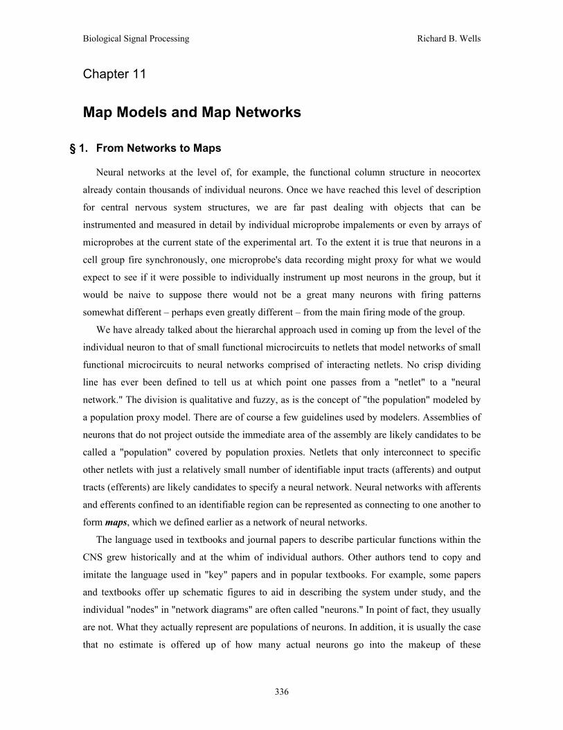
As a specific example, let us look at the network used to describe how higher systems in the

brain co-opt the spinal cord's built-in neural organization of reflexes. Figure 11.1 is a schematic

representation of the spinal cord reflex arc responsible for our reflexes in response to signals

originating from muscle spindles, nerve endings in the peripheral nervous system, etc. Today it is

generally accepted that voluntary movements, commanded by descending signals from the brain,

"take over" the basic neural "circuitry" for involuntary reflexes. It is not too much of a distortion

of the facts to say that the brain's signals "fool" the reflex arc neural networks (or netlets; it is

presently not clear what we should properly call the "circles" in figure 11.1). They stimulate the

pathways converging on the spinal cord's motor neurons and by doing so are able to exert

voluntary control over contraction and relaxation of the skeletal muscles.

It is common for depictions such as figure 11.1 to refer to the connections made by the various

tracts as "synapses." Again, however, the terminology is slightly misleading. The idea intended to

Figure 11.1: Schematic illustration of the reflex arc concept. The circles indicate small networks of neurons at the same synaptic level. IN stands for interneuron. Input signals are actually tracts rather than individual signals. The dashed lines indicate other possible layers of interneurons interposed between the networks shown. The motor commands are descending signals from the reticulospinal and other tracts.

Excitatory pathways are indicated by the "<" symbols. Inhibitory pathways are indicated by the "•" symbol on the lower-left subnetwork. FRA is "flexor reflex afferents", and Lo Th Cut is "low threshold cutaneous

afferents". α-motoneurons are the motoneurons that drive extrafusal muscle fibers. "Early IN" designates interneuron networks that directly receive afferent inputs. "Late IN" designates interneurons at deeper layers in the signal pathway. (These would perhaps consist of neurons in the output layer of the spinal cord dorsal horn or perhaps interneurons in the spinal cord ventral horn). The solid-black network at the upper left in the figure represents mid-level interneurons in the dorsal horn. Note that this network sends inhibitory inputs to the early dorsal horn IN network. It is not clear how many neurons each population in the figure represents,

but none of the "neurons" in the diagram actually represent just one neuron.

337


be conveyed by this terminology is that the members of the neural population have more or less

the same number of neural "relay points" interposed between themselves and the target motor

neurons. This is what is meant by saying the connections are made to the same synaptic level in

the system. Neurons in a population at the same synaptic level are commonly said to constitute a

layer. In the case of the spinal cord, it seems likely to be the case that only a few layers of

neurons are interposed between the afferent signals and the motor neuron layer. We might,

therefore, be inclined to think, "Well, then, these populations are netlets." On the other hand,

many alpha-type motor neurons have tens of thousands of afferents converging on them, and this

seems a bit too many for us to regard the antecedent layers as mere netlets.

Once one becomes aware the diagrams commonly found in the literature do not represent

individual neurons, one might experience a mild sense of indignation that so little quantitative

detail is really conveyed by these diagrams. However, this reaction is unfair to the paper's author.

When someone sets down a lot of detail, the reader can be excused for taking this detail to be

factual, or at least for thinking the author claims it is factual. The paucity of quantitative detail in

such diagrams is an honest reflection of what the medieval scholastic philosopher Nicholas of

Cusa called "learned ignorance." Cusa pointed out it is better to know you do not know

something than to think you know something you really don't. Recognizing and acknowledging

lack of knowledge is learned (pronounced "learn ed") ignorance. The opposite of learned

ignorance is blind ignorance, which is something a good scientist makes a habit of avoiding.

Although our detailed knowledge of the organization of the ventral horn of the spinal cord is

far from complete, it nonetheless seems to be the case that this neural organization is rather "flat."

Figure 11.2: Simplified signal flow pathways to muscles in the ventral horn of the spinal cord. The left-most figure illustrates excitatory pathways to the motor neurons (MN) driving extrafusal muscle fibers (α) and

intrafusal muscle spindles (γ). Groups Ia, II, and III are sensory nerve signals. Joint and cutaneous afferents also provide signals from the peripheral nervous system. The other two figures illustrate Group II inhibitory pathways to the antagonist MN. (A) illustrates the inhibitory pathway for group Ia muscle spindle afferents.

(B) depicts the group II inhibitory pathway, and we can note the similarity between the two figures.

338


Figure 11.2 shows a simplified illustration of part of the ventral horn structure. The spinal cord

receives sensory feedback from the skeletal muscles by means of sensory neurons located in the

intrafusal muscle fibers (group Ia and group II spindle afferents). It also receives sensory

information from other nerves, jointly referred to as flexor reflex afferents or FRAs. The muscle

system is organized in pairs of muscle groups called flexors and extensors. These muscles are

said to form agonist-antagonist pairs because the action of one (e.g. the biceps) opposes the other

(e.g. the triceps). The signal processing in the system provides for inhibition of the antagonist

muscle groups when the agonist muscles are contracting. Experimental studies indicate the

feedforward pathway to the extrafusal muscle for processing the afferent feedback is only a few

layers deep, as suggested in the figure.

The level of detail illustrated by figure 11.2 is typical of what can be recovered by current

practical experimental techniques. For the ventral horn of the spinal cord, measurements are

facilitated by the fact that the signals converge to a common point with a well known function,

namely the motor neurons. For this reason a great deal of information can be obtained by micro-

probe measurements of specific motor neurons. The signal pathway organization in the brain is

less accommodating to our instrumentation capabilities. Here experimental methods capable of

measuring larger-scale neural activity are often such that what is measured is not single-neuron

activity but, rather, the sum of activities from many hundreds or thousands of neurons resolvable

only to a scale on the order of about 1 mm2 of brain tissue. Figure 11.3 [DAMA3] provides an

example of this sort of experimental data. The figure shows positron emission topography (PET)

Figure 11.3: PET scans showing areas of significant activation (deep red) and significant inhibition (deep purple) in human subject during the experiencing of anger [DAMA3].

339


scan data for a human subject during the experiencing of anger. PET scans use radioactive tracers

injected into the blood stream to image changes in blood flow and changes in the metabolism of

glucose. Both of these are indicative of changes in neural activity. Clearly, these changes are

resolvable only on a relatively gross level of neural population.

As you can appreciate, the nature of the signaling data obtained at this level is qualitatively

different from what we have been working with up to this point. The instruments measure signals

indicative of metabolic activity, which is closely related to neuron firing but obviously does not

provide a direct measurement of action potential waveform patterns or pulse timing.

Consequently, the signal models used in map models are also qualitatively different from those

we have seen for neuron-level models and for the spiking population proxy models of the I&F or

Eckhorn type. Instead, the signals represented in map models are continuous-variable quantities

in which the amplitude of the signal represents the level of activity of the map population.

§2. Psychological Objects and Scientific Reduction A map represents a network of neural networks. A network system is a network of maps.

Once we have reached the map level of modeling, we have likewise reached a level where

psychological phenomena provide a much clearer description of system function than do the

biological phenomena we have been dealing with so far in this textbook. Psychological objects

include such things as perception, cognition, consciousness, emotion, and motivation. Unlike

biological phenomena, which can be directly instrumented and largely understood on the basis of

biophysics and physiology, psychological objects are supersensible. That is, they are objects we

know about only because each one of us experiences what is usually termed one's own mental

life. For example, one knows of the phenomenon of "anger" only because each of us knows what

it is "to be angry." Figure 11.3 illustrates a measure of brain-state that corresponds to the feeling

of anger, but figure 11.3 is not a picture of "anger itself." One experiences anger but one neither

sees, hears, touches, tastes, nor smells anger. This is what is meant by saying the psychological

objects are supersensible. Even "experience" as a phenomenon is a psychological object.

The fact that all its objects are supersensible is what makes psychology a more challenging

and difficult science than is physics. Physicists' naive boasting notwithstanding, the objects of

psychology lie completely outside physics' field of competency. There are no "happy atoms" or

"angry electrons" or "pontifical cells." The great German philosopher Immanuel Kant taught that

the sensible physical objects we encounter in the world and the supersensible mental objects we

encounter within one's own self are the two coordinate halves of experience, and they jointly

make up the sum of all one's knowledge of the objects in nature as a whole [KANT].

It is a fundamental tenet of neuroscience that for every psychological phenomenon there is a

340


biological substrate, but this is not the same as saying this biological substrate is the

psychological object. The distinction made between "mind" and "body" is merely a logical

division we each make in our understanding of that integrated object each of us calls "myself."

This is what Kant meant by calling mental life and physical life "coordinate parts"; the whole of

the phenomenon is "me", "myself" as an organized being, incomplete without both the physical

coordinate ("body") and the mental coordinate ("mind"), the "dimensions" of human life.

Piaget has documented the interesting fact that the child's understanding of the world in which

he finds himself begins by the child's endowing to other things the same mental characteristics he

experiences within himself. Indeed, the notion of "physical causality" begins with and proceeds

from the child's growing realization that not everything he encounters bends to his own will.

Indeed, this distinction is provably the point of origin for that ubiquitous division in

understanding all human beings come to make by which each of us distinguishes one's own "self"

from everything else, and by which each of us comes to regard one's own self as an object among

objects in the world.1

Three complementary processes seem to be at work in directing the evolution of reality as it is conceived by the child between the ages of 3 and 11. Child thought moves simultaneously: 1° from realism to objectivity, 2° from realism to reciprocity, and 3° from realism to relativity. By objectivity we mean the mental attitude of persons who are able to distinguish what comes from themselves and what forms part of external reality as it can be observed by everybody. We say there is reciprocity when the same value is attached to the point of view of other people as to one's own, and when the correspondence can be found between these two points of view. We say there is relativity when no object and no quality or character is posited in the subject's mind with the claim to being an independent substance or attribute.

[In] stating that the child proceeds from realism to objectivity, all we are saying is that originally the child puts the whole content of consciousness on the same plane and draws no distinction between the "I" and the external world. Above all we mean that the constitution of the idea of reality presupposes a progressive splitting-up of this protoplasmic consciousness into two complementary universes – the objective universe and the subjective.

All these facts show that the localization of the objects of thought is not inborn. It is through a progressive differentiation that the internal world comes into being and is contrasted with the external. Neither of these two terms is given at the start. The initial realism is not due simply to ignorance of the internal world, it is due to confusion and the absence of objectivity.

This phenomenon is very general. During the early stages the world and the self are one; neither term is distinguished from the other. But when they become distinct, these two terms begin by remaining very close to each other; the world is still conscious and full of intentions, the self is still material, so to speak, and only slightly interiorized. At each step in the process of dissociation these two terms evolve in the sense of the greatest divergence, but they are never in the child (nor in the adult for that matter) entirely separate. From our present point of view, therefore, there is never complete objectivity: at every stage there remain in the conception of nature what we might call "adherences", fragments of internal experience which still cling to the external world.

1 Children with severe autism have difficulty in making this distinction, and it is known that this difficulty is related to brain pathology. Very special care-giving is needed to help them overcome this condition.

341


The second characteristic process in the evolution of the idea of reality is the passage from realism to reciprocity. This formula means that the child, after having regarded his own point of view as absolute, comes to discover the possibility of other points of view and to conceive of reality as constituted, no longer by what is immediately given, but by what is common to all points of view taken together.

One of the first aspects of this process is the passage from realism of perception to interpretation properly so called. All the younger children take their immediate perceptions as true, and then proceed to interpret them according to their egocentric pre-relations, instead of making allowance for their own perspective. The most striking example we have found is that of the clouds and heavenly bodies, of which children believe that they follow us. The sun and moon are small globes traveling a little way above the level of the roofs of houses and following us about on our walks. Even the child of 6-8 years does not hesitate to take this perception as the expression of truth, and, curiously enough, he never thinks of asking himself whether these heavenly bodies do not also follow other people.

These last examples bring us to the third process which marks the evolution of the child's idea of reality: thought evolves from realism to relativity. . . The most striking example of this process is undoubtedly the evolution of conceptions about life and movement. During the early stages, every movement is regarded as singular, as the manifestation, that is, of a substantial and living activity. In other words, in every moving object is a motor substance: the clouds, the heavenly bodies, water, and machines, etc., move by themselves. Even when the child succeeds in conceiving an external motor . . . the internal motor continues to be regarded as necessary. . . But later on, the movement of every body becomes the function of external movements, which are no longer regarded as necessary collaborators but as sufficient conditions. . . In this way there comes into being a universe of relations which takes the place of a universe of independent and spontaneous substances [PIAG12: 241-250].

None of us can actually "get inside another person's head," but experience does not gainsay

our conception of other people as possessing the same sort of mental life we each ascribe to our

own self. "Mental telepathy" is no part of human nature and so we must try to understand

psychological phenomena through observable behavior and psychophysical correlates to

behavior. This is what we do with network system models. The map models of which these

systems are composed are steps taken in scientific reduction from psychological phenomena

toward neuropsychological theory. As you have perhaps already realized, when we work at the

level of network system and map models, computational neuroscience is no longer headed in the

direction of model order reduction ascending the hierarchy of scientific levels of understanding

but, rather, is engaged in descending the ladder to make a connection of understanding between

psychological life and biological life, the two coordinates of human life.

§3. The Instar Node The oldest and, judging from the bulk of the literature, most popular map model originated

with Rosenblatt and, independently, with Widrow in the late 1950s and underwent development

into its present-day form in the 1980s. It has come to be known by many names. We will call it

the Instar node. Others call it the sigma node. Many refer to it as the generic connectionist

neuron (GCN). Outside the field of neuroscience proper, e.g. in the field of artificial and

342


engineering neural network research, this model is often just called a "neuron," but we are in a

position to accurately understand that this model represents very large, functional neural/glial cell

populations. Rumelhart, McClelland, et al., who are widely credited with forging the rebirth of

wide-spread neural network research in the United States in the late 1980s, merely call it the

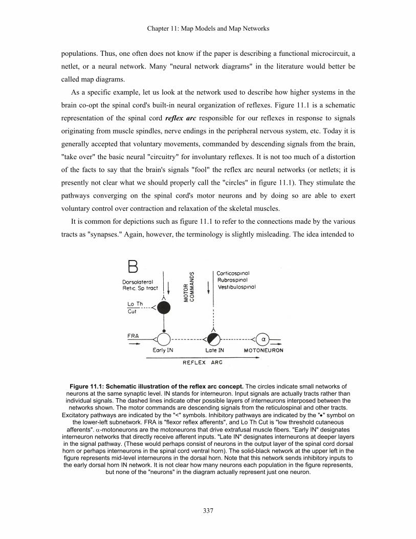
processing unit of a parallel distributed processing (PDP) model [RUME2: 45-76]. Figure 11.4

illustrates the mathematical form and schematic symbol of the Instar node. Rosenblatt's

perceptron and Widrow's Adaline are two special cases of the Instar node. Many authors ignore

all fine distinctions among the different mathematical species of Instar nodes and merely refer to

any map of this general class as a perceptron.

In the usual case, the inputs xi, weights wni, internal excitation variable sn, and output yn are

real-valued continuous variables. The xi and yn represent activation levels ("activation" for short).

The concept of an activation level is an abstract concept meant to convey in some sense "how

active" a network represented by an Instar node map is. The inputs xi usually represent either

outputs of other Instar nodes or the intensity of input stimuli arriving from some external source.

One of the earliest conjectures on the putative "neural code," dating back to von Neumann's work

in the 1940s and 1950s, proposed that information in biological neural networks was represented

by the firing rates of individual neurons. Thus it was natural to view the level of activation of a

neuron as some monotonic function of its firing rate, and so the activation level of an Instar node

is even today called a firing rate by many authors and the Instar node is consequently also known

by some as the firing rate model. In view of the great many things neuroscience has learned since

the 1950s, today this view of what an activation level represents seems simplistic and naive.

While the notion of activation as firing rate perhaps provides a comforting mechanistic analogy of

Figure 11.4: Mathematical form and schematic symbol of the Instar node.

343


what the more abstract idea of activation level means, it is an analogy that tends to lose any clear

meaning once one has realized what an Instar node in a network system model represents. For

this reason, it is better to discard the view of activation-as-firing-rate and merely regard it as some

quantitative measure of the gross metabolic state of a region of neural tissue. Regarding it in this

fashion provides a more faithful context with experimental data obtained by methods such as the

PET scans shown in figure 11.3.

The excitation level of the node is defined to be the weighted sum of input activations,

(11.1) XWTn

N

iinin xws =⋅= ∑

=1

where Wn and X are vectors corresponding to the weights and input signals, respectively. The

output activation level of the node is some (usually nonlinear) function of the excitation level,

. (11.2) ( nnn sy g= )

The specific mathematical expression used for the activation function specifies what

particular species of Instar node is being used. The simplest case is where is merely a

Heaviside step function with threshold

ng

gn

g . ( )

Θ>Θ≤

=n

nnn s

ss

,1,0

For the special case where the xi are binary-valued, with values 0 and 1, all the weights wni = ±1,

and gn is the step function, the Instar node reduces to the general McCulloch-Pitts neuron model.

In this sense, the digital computer can be regarded as a network system comprised of McCulloch-

Pitts Instar nodes. In the original Adaline model, g was a signum function, = sgn(sn ng n – Θ),

which produces an output of +1 if sn – Θ > 0, –1 if sn – Θ < 0, and 0 if sn – Θ = 0. Rosenblatt's

perceptron was similar [WIDR3], [ROSE3]. Other popular activation functions include:

the unipolar sigmoid function, ( ) ( )uun ⋅−+=

αexp11g ;

the bipolar sigmoid function, ( ) ( )uun ⋅= αtanhg ; and

the radial basis function, ( ) ( )2expg uun ⋅−= α

where in the general case u = sn – Θ and α > 0 is a parameter controlling the maximum slope of

the function. Other activation function are also used, but these are the most popular in practice.

344


Note that the unipolar sigmoid and radial basis functions limit yn to the range from 0 to +1, while

the bipolar sigmoid limits it to the range –1 ≤ yn ≤ +1.

§3.1 Geometric Interpretation of the Instar Node As may already be apparent, the Instar node is a model operating at a very high level of

abstraction. As a mathematical element of a network system, modeling work employing it is of a

functional rather than physiological nature, and here it is important for the modeler to have a way

of visualizing and interpreting what the model is doing. Fortunately, there is a simple geometrical

interpretation of Instar function that can be applied for all the activation functions introduced

above except for the radial basis function.2

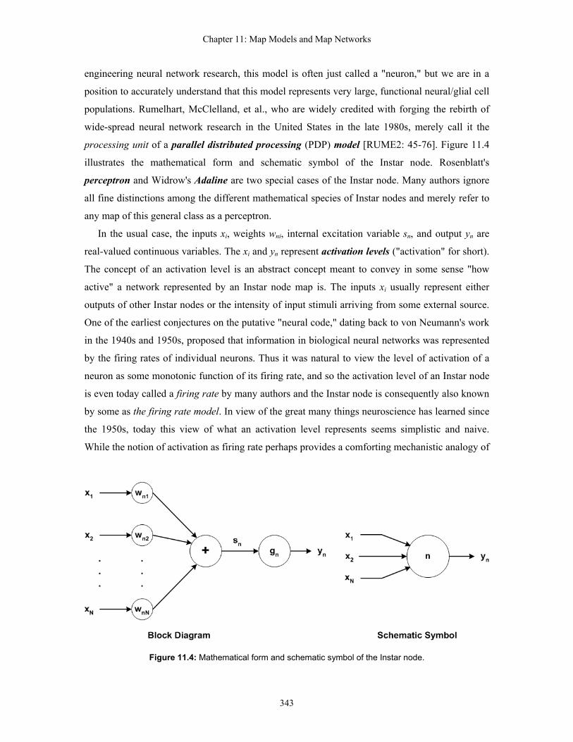
Without loss of generality, we will let u = sn – Θ. Clearly u is a linear function of the inputs xi.

The equation

u (11.3) 01

=Θ−⋅= ∑=

N

iii xw

defines what is called a separating boundary in the Euclidean metric space for which the xi are

regarded as the coordinates of the space. This idea is illustrated for the two-input case in Figure

11.5. The separating boundary is merely a straight line partitioning the plane defined by x1 and x2

into two regions. On this separating line we have

2

12

12 w

xwwx Θ

+⋅−= .

Figure 11.5: Illustration of a two-dimensional separating boundary. The signs of u correspond to w2 < 0.

2 We will see later that the radial basis function has a topological interpretation. This, too, is a geometrical interpretation in the general sense of that term, but it differs from what is being presented here.

345


Intersect a is given by a = Θ/w1, and intersect b is given by b = Θ/w2. (Figure 11.5 therefore tells

us that in this example we have opposite signs for parameters Θ and w2). The slope of the

separating boundary line is merely –w1/w2. (The positive slope of the line in figure 11.5 therefore

tells us w1 and w2 also have opposite signs for this example).

Values for coordinate x2 such that w2x2 < –w1x1 + Θ correspond to values of u < 0. In the

example figure, this is the region above and to the left of the separating line. Values for

coordinate x2 such that w2x2 > –w1x1 + Θ correspond to u > 0 (below and to the right of the line in

figure 11.5). Values x1, x2 corresponding to u = 0 are typically regarded as the baseline activity

level of the Instar node, thus the separating boundary partitions the input space defined by

coordinates x1, x2 into a below baseline region and an above baseline region. Since baseline

activity is generally regarded as a basic reference level, below-baseline activation implies the map

is relatively inactive, i.e. inhibited, while above-baseline activation implies the map is relatively

active, i.e. excited. Thus, the separating boundary defines two distinguishable regions of

activation.

Because each Instar has its own separating boundary defined by its threshold and weights,

multiple nodes in a network system can be used to partition the input space into multiple regions

(subspaces). Figure 11.6 illustrates this for our two-input example. Instar nodes 1 to 3 perform the

spatial partitioning. Figure 11.6(A) illustrates one possible partitioning. Each region is defined by

the combinations of conditions un < 0 or un > 0. For the example shown, the x1, x2 space is

divided into seven regions. By appropriate choices of threshold and weights for the Instar node in

Figure 11.6: Two-layer neural network system partitioning the input space into seven regions and responding to inputs in one of these regions. (A) Input space partitioning. (B) Network system.

346


the second layer in figure 11.6(B), the network system can be made to respond (become relatively

active) to just those inputs falling into one specific subspace and to be inactive for inputs in the

others. The network system is therefore said to classify input signals. The system shown in figure

11.6 is an example of a two-layer feedforward neural network system, more commonly called a

two-layer feedforward neural network.

§3.2 Feedforward Instar Network Systems as Function Generators Instar number 4 in figure 11.6(B) can select any one of the seven regions shown in figure

11.6(A) or it can select the union of adjacent regions definable by ignoring any one or any two of

the separating boundaries defined by the Instars in the first layer. For example, Instar 4 could be

set up to respond only to region 1 in the figure. Or, by ignoring Instar 2, it could respond to the

union of regions 1 and 6. (This would amount to setting weight w4,2 = 0 in Instar 4). However, it

could not be set up to respond to, for example, the union of regions 3 and 6 because the

separating boundary conditions are opposite for these two regions. Note that both region 3 and

region 6, considered individually, form convex shapes in the input space. The union of regions 3

and 6 produces an overall region that is not convex; such a region is said to be "arbitrary."

Suppose we added another Instar (Instar 5) to the second layer, such that Instar 4 responded to

region 3 and Instar 5 responded to region 6. We could then add another Instar in a third layer,

Instar 6, fed from Instars 4 and 5. If Instar 6 responded if either Instar 4 or Instar 5 showed

relative excitation, then the overall network system would respond with relative excitation to

inputs falling into the union of regions 3 and 6. It has been shown that a three-layer feedforward

neural network system can classify input signals for arbitrarily-shaped shaped regions of its input

space. Thus, in principle, a three-layer feedforward neural network system can solve any

classification problem. It is for this reason often called a universal function generator.

If we extend this example to three input variables, the separating boundary becomes a plane in

the three-dimensional space defined by the input variables. This is, not surprisingly, called a

separating plane. When we go to four or more input variables, the separating boundary is called a

separating hyperplane. At this point, our ability to picture the input space graphically is outrun by

the dimensions of the input space. Nonetheless, the geometrical arguments made above for the

two-input case hold up for any m-input input space. A two-layer feedforward neural network

system can classify any convex region of the input space as well as some types of non-convex

regions [GIBCO]; a three-layer system can classify any arbitrary region of an m-input input

space.

In most cases, for a feedforward network system to distinctly classify M simple convex regions

in an input space, the second layer of the network must contain M Instars (one for each convex

347


region). If we allow the minimum and maximum values of the input signals to serve as default

boundaries for the input space, then a minimum of one first-layer Instar is required to form a

convex region (this region will be a simple hyper-half-plane), and a maximum of three Instars can

suffice to form a more general convex region. If we wish to have a closed convex region not

bounded by the range of the input variables, we must then have at lease four Instars in the first

layer to define the region in a three-input space (a tetrahedron has four sides, three faces and a

base, and so requires four intersecting planes). This is thought to be true also for m > 3, although

difficulties attending the combinatorics of hyperplanes make this less certain [GIBCO].

The combined effect of the nodes in a two-layer Instar network is to partition up the input

space into regions of hyper-polyhedral shapes. This is called segmentation of the input space and

is something Instar networks do very well. To form more complex classifications from the union

of two or more convex segments requires no more than the addition of a third layer in the

network. Consider again the PET scan image shown earlier. If one wished to have a network of

Instar nodes capable of classifying "anger" by recognizing the pattern of red and purple regions

shown in the PET scan, then in principle a three-layer Instar network could do the job provided

the weights and thresholds of the Instars could be set with unlimited precision.

Now, as a practical matter unlimited precision is not something obtainable using real

calculations in a computer. All computers have finite precision. When we consider a system

comprised of neurons, unlimited precision is even more so an unrealizable ideal. As we have seen

in the earlier chapters, the "precision" of neural mechanisms for signal processing have accuracies

of at best a few percent, on the order of perhaps about three decimal digits [NEUM3]. How much

precision is required for arbitrary classification tasks?

There is at the present time no general theorem that answers this question. However, there is

such a theorem for the case of the relatively primitive perceptron networks of the 1960s. It was

provided by Minsky and Papert [MINS], and we shall refer to it as the Minsky-Papert

stratification theorem. The details of this theorem are far too mathematically sophisticated to

present in this textbook, considering its target readership, but the result is easy to state. As the

number of convex regions that must be distinguished increases, the precision required of the

parameters of the network system increases at a geometric rate (or worse!). It means, for example,

that if the number of convex regions to be classified doubles, the precision requirements increase

more than two-fold. (In computer language, doubling the number of regions requires an addition

"bit" – binary digit – of accuracy in the weight and threshold values).

This, of course, does not apply to every possible classification problem, but it is not hard to

find problems that exhibit this undesirable requirement. For 1960s-era perceptron networks the

348


stratification theorem is a theorem (that is, it was proved). The conditions going into the proof of

this theorem are not the same conditions found in modern multi-layer Instar networks, but this

does not mean the stratification theorem is false for the modern networks. There is a big

difference between "not proved" and "false." There is evidence, both empirical and theoretical,

warning we not gotten away from the limitations of the Minsky-Papert stratification theorem

merely because Instar networks are better than 1960s perceptron networks [WIDR4]. This issue

remains open pending the discovery of a theorem to settle it once and for all. The question,

however, provides a sufficient degree of reasonable doubt to merit hesitation in calling Instar

networks "universal function generators" in a practical sense.

Having said this, the other side of the story is that, for sufficiently "small" segmentation and

classification problems, Instar networks have proven to be remarkably versatile and successful in

a great many cases. In the world of neural network engineering – that is, in the field of artificial

neural networks used for practical engineering applications outside the field of neuroscience – the

Instar network is the most widely used type of network and has been usefully applied to a great

many practical engineering problems. The relevant question for us in this textbook is: To what

extent can the Instar network be regarded as a biologically-realistic way to model and represent

functions in the central nervous system?

Each Instar in the final or "output" layer of a feedforward Instar network is sometimes called a

"grandmother cell" – as in when Instar n is relatively active, the network "recognizes grandma."

For many years theoretical neuroscience worked on the hypothesis that "grandmother cell" neural

architecture was a more or less accurate model of brain function. This view was seen as

consistent with the supposition that more and more sophisticated cognitive abilities accrued as

signals flowed from the sensory cortices "forward" to downstream association cortices (where

different sensory modalities were thought to be combined) and, from there, on toward the frontal

lobe where "higher cognitive and reasoning functions" were thought to first be realized. This is

known as the "caudal-to-rostral flow" model of information processing in the brain. There are at

least two reasons why the caudal-to-rostral "grandmother cell" model has to be rejected.

The first reason is mathematical and is known as the combinatorial catastrophe. Grandmother

cell responses are very, very specialized and one is needed for each specific individual

"recognition" to be made. If we regard each output node in an Instar feedforward network as the

output of a function taking input vector X to a simple binary response ("yes" or "no"), as the

number of convex regions going into the "combinatorial encoding" of the response increases, the

number of Instars required increases faster than geometrically. It would take only a surprisingly

small degree of complexity in the recognition task to require the number of grandmother cells to

349


outnumber the total number of neurons in the brain! For example, the grandmother cell scheme

requires a grandmother cell for "grandma in the kitchen," another for "grandma in the car," a third

for "grandma with grandpa at the table," etc. Quite apart from the disastrous effect the death of a

grandmother cell would have on one's cognitive abilities, encoding by grandmother cells is a

hopelessly inefficient model of cognitive function.

There is also a neurological reason for rejecting the caudal-to-rostral information flow model.

It makes predictions concerning the effects different types of brain injuries should have on the

patient's cognitive abilities, and these predictions are found to be false. Damasio has provided a

number of case study findings in which implications of the caudal-to-rostral model are

contradicted by studies of what effects patients do and do not exhibit in response to specific

pathologies [DAMA1]. These studies underlie Damasio's convergence zone hypothesis

[DAMA1-2], and while they are not sufficient to unequivocally establish Damasio's hypothesis as

a fact, they are decisive for rejecting the traditional caudal-to-rostral flow model.

However, all this does not necessarily mean the feedforward Instar network is not an adequate

model on a sufficiently small scale, e.g. for small maps representing cooperative actions among a

few neocortical functional columns. Functional columns do appear to be rather specialized in

their tasks, and data obtained by methods such as subdural probes 3 do show a noticeable degree

of signal correlation taking place among nearby neighboring regions of cortex.

§4. Competitive Networks

A feedforward Instar network is said to be a "memoryless" network because the input-to-

output function it implements is strictly combinatorial. Memoryless systems are systems that can

be described without resort to state variables because the response of the system at the next time

step in no way depends on any prior signals previous to this time step. Another way to describe

this is to say the network lacks feedback or is non-recurrent.

Feedback is ubiquitous in the central nervous system. At all modeling levels from the netlet on

up, we find lateral feedback connections between structures on the same synaptic level and

retrograde feedback from "downstream" structures back to the "upstream" structures projecting to

them. The linking field function we saw previously in the Eckhorn model is one example of this,

and Eckhorn-model-based networks frequently use the linking field for lateral connections within

a single layer, and for feedback connections in multiple-layer networks. Damasio's network

3 The dura is a thick fibrous membrane lining the inside of the skull and covering the vertebrate brain. Subdural implants are probes place in or slightly below the dura. These probes pick up combined electrical signals from the thousands of cortical neurons located just below them. Arrays of subdural implants do show a spatially-limited region of reasonable correlation between adjacent probes [BRUN].

350


(figure 9.4) is another example. The presence of feedback in a network is dramatic. It introduces

the element of temporal signal processing into the dynamics of the system. Feedback makes

possible the implementation of functions by a relatively small number of elements that would

otherwise require an enormous number of elements in a combinatorial network.

One common and useful network structure utilizing lateral feedback connections is depicted in

Figure 11.7. This single-layer map network is called a competitive network. Each node in the

layer is an Instar map. Each Instar makes a projection to every Instar in the layer and, in return,

receives a projection from every Instar, including itself. (The figure illustrates this only for node n

in order to save cluttering up the figure). Often (but not always), each node receives only a single

input signal xn from outside the layer. In this case, each node receives a maximum of N + 1

inputs, where N is the number of nodes in the layer. Network connection is described by an N × N

matrix W, where each row n of W represents the weight vector Wn of the nth node. The rows are

sometimes called the "footprint" of the nodes' connection weights.

§4.1 The MAXNET

Perhaps the simplest version of a competitive layer is the MAXNET. This network

implements what is known as a winner-take-all (WTA) function. Once the layer has settled into a

steady-state response condition, every node except one (the "winner") is completely inactivated.

The activation level of the "winning" node is a reflection of "how close the competition was,"

with a small activation level if the competition was "close" and a larger activation if the "margin

of victory" was large. In the event of a "tie," every node in the layer is inactivated. The winner

will be the node receiving the largest excitation from an initial stimulus xn. Thus, the MAXNET

functions as a comparator for a bank of incoming stimuli.

Figure 11.7: Schematic illustration of a competitive layer. Each node is an Instar. Every node makes a reciprocal connection to every other node in the layer. The figure illustrates this only for node n. In a wrap-around configuration, nodes at the ends of the layer treat the nodes on the opposite side as if they were

neighbors within a "radius" of r nodes. Such a configuration is often called a "ring" configuration.

351


The most common activation function for the Instars in a MAXNET is the linear threshold

function with threshold Θ = 0,

g ( )nnn ss H⋅=

where H is the Heaviside step function. The weight matrix W of the competitive layer is

symmetric with diagonal elements wnn = 1 and off-diagonal elements wni = –ε, i ≠ n, i ∈ [1, N].

Here ε is a small positive constant in the range 0 < ε < 1/N.

The MAXNET is operated in competitive cycles we will call tournaments. Let t0 denote the

time index at the start of a tournament. The activations of every node are initialized to yn = 0 at

time index t = t0 – 1 for all nodes in the network and the external stimuli X are applied at t = t0.

To obtain a mathematical expression for the network dynamics, we introduce the Kronecker delta

function

. ( ) =

=−otherwise,0

,1 00

ttttδ

The tournament runs from time index t0 to time index t0 + T, where T is a sufficiently large

number of time steps for the MAXNET to converge to a single winner. Typically values of T in

the range of 15 to 20 are usually sufficient. The dynamical equations for the network during the

tournament are

( )( )

( )

( ) ( ) ( ) ( ) ( )

( )( )( )( )

( )( )

=+⋅−+⋅==

ts

tsts

tttttt

ts

tsts

NN g

gg

1; 2

1

02

1

MMYXYWS δ . (11.4)

Here X = [ x1 . . . xN]T. Note that external stimuli X are disabled during the tournament except at

the initial time index t0. This is absolutely necessary to ensure the stability and convergence of the

MAXNET. Note also that since Y(t0) = 0, the tournament begins by "forgetting" the outcome of

the previous tournament. This, too, is necessary to ensure proper operation of the winner-take-all

competition.

Figure 11.8 illustrates a MAXNET competition for N = 5 nodes and an initial stimulus vector

X = [0.8 0.95 0.81 0.9 0.82]T. The weight matrix W used ε = 0.5/N = 0.1 for setting the off-

diagonal elements. The tournament was run for T = 20 time steps, and it is easily seen that all

nodes except winning node Instar 2 have converged to zero by the 14th time step of the

tournament. The relatively low final activation of the winning node is due to the fact that the

input stimuli were relatively close to one another at t = t0.

352


0 5 10 15 200

0.2

0.4

0.6

0.8

1

node 1node 2node 3node 4node 5

Activations vs. Competitive Time Index

Y t⟨ ⟩( )0

Y t⟨ ⟩( )1

Y t⟨ ⟩( )2

Y t⟨ ⟩( )3

Y t⟨ ⟩( )4

t

Figure 11.8: MAXNET competition for N = 5 nodes with ε = 0.5/5.

One can also note that the three nodes receiving nearly-equal non-winning stimuli, Instars 1, 3,

and 5, have nearly equally rapid decay to zero. It is a general feature of the MAXNET that nodes

receiving almost-equal stimuli will show very similar time courses until the point is reached

where a clear winner begins to emerge from the competition. The smaller the final activation of

the winning node, the less difference there was among the initial stimuli. If two or more nodes

receive equal highest stimuli, no winner will result and all the nodes will decay to a zero

activation.

Although the device of "turning off" the external stimuli after the tournament begins may

seem both very artificial and non-biological, this is not necessarily the case. Earlier in this text

when synapse configurations were discussed, it was noted that axo-axonal synapses were

frequently inhibitory. This is called presynaptic inhibition. It is known that presynaptic inhibition

occurs in many areas throughout the central nervous system. For example, there is significant

presynaptic inhibition found in dorsal horn networks of the spinal cord. (The dorsal horn is the

input port for signals coming in from the peripheral nervous system). There are likewise known

cases of presynaptic inhibition found in neocortex. Therefore, while turning off the input stimuli

of the MAXNET after the tournament begins is a mathematical necessity, it is not necessarily an

353


un-biological device.

§4.2 The Mexican Hat Network

Another competitive Instar network, also illustrated by figure 11.7, that finds wide use in

network system modeling bears the curious name "Mexican Hat network." This network belongs

to the class of laterally-recurrent networks generally called contrast enhancing networks and,

more specifically, called on-center/off-surround networks. The name comes from the shape of

the graph of the weight footprint for the Instar nodes. Each node feeds back to itself with an

excitatory weight connection wnn that has the largest magnitude of all its connecting weights.

Nodes within a "distance" of L1 neurons of node n are projected to with smaller excitatory

weights, typically decreasing with increasing distance. Nodes within a distance L1 < L ≤ L2 are

projected to with inhibitory weights, typically decreasing in magnitude with increasing distance.

Nodes at distances greater than L2 receive no projection from node n (wmn = 0). The weight matrix

W is symmetric. Folklore in the neural network community has it that renowned Finnish neural

network theorist Teuvo Kohonen thought this weight footprint resembled a sombrero and so he

called it a "Mexican hat." Whether this is the true source of the name or not, Kohonen used it in

print and the name has stuck ever since.

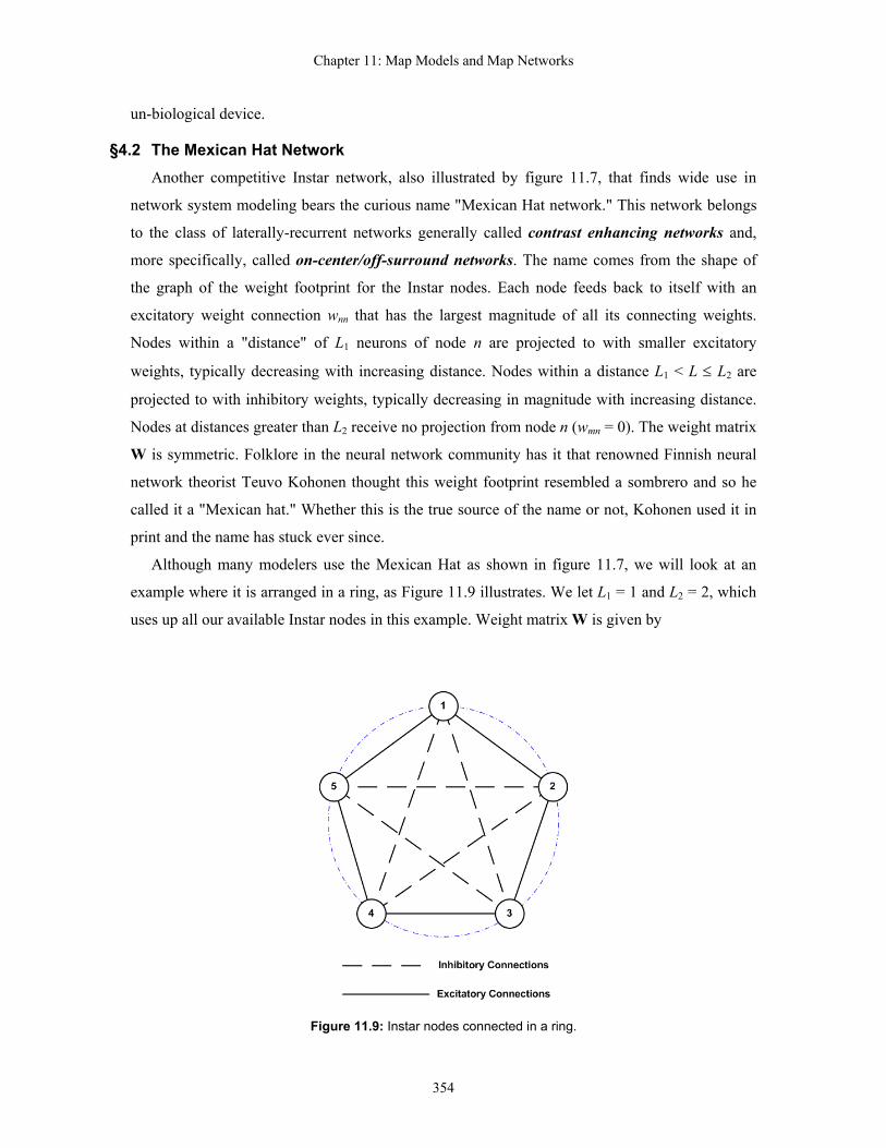
Although many modelers use the Mexican Hat as shown in figure 11.7, we will look at an

example where it is arranged in a ring, as Figure 11.9 illustrates. We let L1 = 1 and L2 = 2, which

uses up all our available Instar nodes in this example. Weight matrix W is given by

Figure 11.9: Instar nodes connected in a ring.

354


0 5 10 15 200

0.2

0.4

0.6

0.8

1



Y t⟨ ⟩( )0

Y t⟨ ⟩( )1

Y t⟨ ⟩( )2

Y t⟨ ⟩( )3

Y t⟨ ⟩( )4

t0 5 10 15 200

0.2

0.4

0.6

0.8

1



Y t⟨ ⟩( )0

Y t⟨ ⟩( )1

Y t⟨ ⟩( )2

Y t⟨ ⟩( )3

Y t⟨ ⟩( )4

t

A B

Figure 11.10: Tournament response for Mexican Hat example with N = 5, r = 0.7, ε1 = ε2 = 0.3. (A) stimulus vector X = [0.75 0.98 0.86 0.79 0.67]T. (B) stimulus vector X = [0.67 0.98 0.86 0.79 0.75]T.

.

−−−−

−−−−

−−

=

rr

rr

r

1221

1122

2112

2211

1221

εεεεεεεεεεεεεεεεεεεε

W

The network equations are given by (11.4), i.e. they are the same as for the MAXNET. A

common activation function used for the Mexican Hat is the saturating linear threshold function,

g . ( )

≥<≤

<=

maxmax

max

,0,

0,0

xxxxxx

xxn

Figure 11.10 provides two examples of the Mexican Hat response. Parameters and input

stimulus vectors are provided in the figure caption. Both simulations use the same network

parameters and differ only in that the stimuli for nodes 1 and 5 are swapped. (Referring to figure

11.9, nodes 1 and 5 are considered "adjacent" to each other). In both cases node 2 receives the

largest external stimulus.

The first observation we can made is that the final state of the tournament differs for the two

cases. What this means is the response of the network is initial condition dependent (i.e. depends

on X at the t = t0 initial time step). This happens because the activation function is a nonlinear

function; linear and time-invariant systems would not have a final response that depends on the

355


initial condition. Indeed, if this example network had been a linear network, its dynamics would

have been unstable and the node responses would have grown without bound.

The next difference to note is between the final values of the tournament. In figure 11.10(A),

the winning node is node 2 (which received the largest stimulus), but its excitatory neighbors,

nodes 1 and 3, also have non-zero, albeit lower, final values. In contrast, the winning node in

figure 11.10(B) is not node 2 but rather node 3. Although node 2 still has the largest direct

stimulation, the total initial stimulation for node 3 and its on-surround, nodes 2 and 4, is greater

than for node 2 and its on-surround (nodes 1 and 3). A quick check for case (A) shows this to be

true there as well: node 2 and its on-surround had a larger initial stimulus than node 3 and its on-

surround. The tournament winner for the Mexican Hat is not the node receiving the largest

stimulus but, rather, the "center" node of the on-surround receiving the greatest overall initial

stimulus. The tournament is not "winner-take-all"; rather, the non-zero-responding nodes at the

end of the tournament identify a region of greatest stimulus.

The presence of positive off-diagonal terms in W means the Mexican Hat network contains

positive feedback connections. This means that, unlike the MAXNET, the Mexican Hat network

is unstable for some combinations of connection weights. Figure 11.11 illustrates two cases of

instability in the Mexican Hat network of our previous examples. X is the same as was used in

figure 11.10(B). The values of the wij are given in the caption. It is clear that no non-saturating

fixed-point solution develops in either case during the tournament. The general stability problem

for the Mexican Hat network is a problem in nonlinear dynamics, and so a simple statement of the

0 5 10 15 200

0.2

0.4

0.6

0.8

1



Y t⟨ ⟩( )0

Y t⟨ ⟩( )1

Y t⟨ ⟩( )2

Y t⟨ ⟩( )3

Y t⟨ ⟩( )4

t0 5 10 15 200

0.2

0.4

0.6

0.8

1



Y t⟨ ⟩( )0

Y t⟨ ⟩( )1

Y t⟨ ⟩( )2

Y t⟨ ⟩( )3

Y t⟨ ⟩( )4

t

Figure 11.11: Two unstable responses for the Mexican Hat with X = [0.67 0.98 0.86 0.79 0.75]T, xmax = 1. (A) r = 0.75, ε1 = ε2 = 0.3. (B) r = 0.7, ε1 = 0.31 ε2 = 0.3.

356


stability conditions for the network is not forthcoming. For our example network, parameter

choices satisfying r > ε1, ε1 = ε2, and r + ε1 = 1 tend to result in stable network responses, but this

does not generalize to other Mexican Hat networks in a straightforward way.

Although general design rules for the Mexican Hat are not straight-forward, there is a test one

can make to determine if a particular weight "footprint" will produce suitable results. It is based

on the submatrix V of weight matrix W obtained by picking one of the nodes as the "center" node

and including the 2R1 nodes in its excitatory surround. For the example system above, we select

node 3 (the centermost node) and the two adjacent nodes in its surround. Extracting the rows and

columns corresponding to these nodes (nodes 2, 3, and 4) from W we obtain

.

−

−=

rr

r

12

11

21

εεεεεε

V

Like W, submatrix V is a symmetric matrix.

Now, if W for the Mexican Hat produces stable, non-saturating fixed points there will come a

point in the tournament when the winner's off-surround nodes in the network will have decayed to

produce zero-valued outputs. In this case the tournament dynamics are given by the reduced set of

equations governing the winning node and its on-surround.

. ( )( )( )

( ) (tttytyty

YVY ′⋅=+′≡

+++

1111

4

3

2

)

which is a homogeneous difference equation. If stable fixed-point solutions exist, then as t → ∞

we will have

. YVY ′⋅=′

The initial conditions for this equation will depend on the initial external stimulus and on the

state of the Y vector at the time when all the off-surround nodes have decayed to zero. Without

loss of generality, we can take this time step to be t = 0 in our difference equation. Provided all

nodes in the on-surround and the center node remain in the linear region of the activation

function, the general solution of the difference equation is easily shown to be

. ( ) ( )0YVY ′⋅=′ tt

Because V is a symmetric matrix, there is an easy method for seeing how this solution evolves

over successive time steps. The method works by diagonalizing the V matrix. An n × n matrix is

357


characterized by n scalar constants called its eigenvalues. The eigenvalues of a matrix are scalar

solutions for the characteristic equation

0=−VIλ

where I is the identity matrix and λ is the eigenvalue. Standard computer software packages such

as Mathcad® contain routines for finding the eigenvalues of a matrix. Associated with each eigen-

value is a characteristic vector Ψ called its eigenvector for which

ΨΨV λ=⋅ .

The matrix Q whose columns are the eigenvectors of V, e.g.,

Q [ ]432 ΨΨΨ=

is called the modal matrix of V. When V is a symmetric matrix, the modal matrix has the

property

Q .

≡=−

4

3

21

000000

λλ

λΛVQ

Now let us make a change of variables Ω . This is called a similarity

transformation and is a useful trick for doing linear algebra. Substituting into the solution for our

difference equation and rearranging terms gives us

QΩYYQ =′⇒′≡ −1

( ) ( ) ( )001 ΩΛQΩVQ ttt == −Ω

where the equality between the middle and right-most terms is easily verified.

This result tells us the stability and steady-state properties of the solution are determined

solely by the eigenvalues of V. If any eigenvalue is such that λ> 1, the Mexican Hat network is

unstable. If all eigenvalues are such that λ< 1, then the outputs of all the nodes will decay to

zero, another undesirable result. If any one (or more) eigenvalue is λ = –1, the Mexican Hat will

oscillate with a bounded oscillation. Therefore, a desirable set of weights will be such that the Λ

matrix will have a form equivalent to

=

400010001

λΛ

with λ4< 1. "Equivalent to" means Λ can be put in this form through elementary row-column

358


operations. In this case, we have

→

∞→000010001

lim t

tΛ

and a fixed-point steady-state solution exists. Note that one of the yn solutions will be dependent

on the others because the bottom row of the matrix above is all-zeroes. For best results, Λ should

contain at least two eigenvalues equal to 1 to avoid excessive attenuation of the tournament

results. Note, too, that the theoretical result we have just derived ensures that the stability of the

Mexican Hat network does not depend on the initial stimulus it receives, although obviously the

final output of the network does.

§5. Recurrent Instar Networks With the exception of only a relative few network systems, some of which we will encounter

in the chapters to follow, the theory of multiple-layer Instar networks with feedback is not highly

developed. This is because the combination of feedback from downstream layers and the non-

linear activation function of the Instar node presents very formidable mathematical difficulties.

This is in contrast to neural network models constructed using Eckhorn models, where the

feedback from downstream layers is often limited to just the linking fields (we recall that the

linking field by itself cannot produce an action potential response from an Eckhorn model) or is

inhibitory. Still, there are a few general properties of recurrent Instar networks we can discuss.

We close out this chapter by looking at these. We will confine the discussion to Instar nodes

using the bipolar sigmoid activation function, although most of what we cover here also applies to

Instars that use the unipolar sigmoid function. We will further confine the discussion to Instar

networks that do not contain embedded competitive layers such as the MAXNET or the Mexican

Hat. These layers are usually used to separate different network subsystems within a larger

system and for implementing unsupervised learning algorithms, which we discuss later.

We assume an arbitrary Instar network comprised of N Instar nodes, labeled 1 to N. Each

Instar is assumed to have some threshold Θn and a 1 × N row vector Wn of weights, some of

which can be zero, defining its interconnections with the other nodes in the network. We assume

the network has p external inputs distributed to each Instar through a set of input weights

described by a 1 × p row vector Bn called the Instar's input distribution weight vector. As before,

each Instar has an excitation variable sn and an output variable yn, which we conveniently gather

together in N × 1 vectors S and Y, respectively. We let g denote the bipolar sigmoid activation n

359


function for the nth Instar. Recalling that is defined by the threshold and the slope parameter

α

ng

n, each Instar can have its own specific activation function by allowing these parameters to be

different for different nodes.

At each time index t the outputs of the N Instar nodes are given by

or, more compactly, Y(t) = G(S(t)) (11.5a)

( )( )

( )

( )( )( )( )

( )( )

Θ−

Θ−Θ−

=

NNNN ts

tsts

ty

tyty

g

gg

222

111

2

1

MM

where we introduce the G notation as a convenient abbreviation for the activation functions of the

network. We define the network weight matrix and input distribution matrix using the row vectors

defined above. We have

=

=

NN B

BB

B

W

WW

WMM

2

1

2

1

, .

With this notation, the network dynamics are then given by the system of difference equations

S (11.5b) ( ) (ttt XBYW ⋅+⋅=+ )(1 )

where X is the p × 1 column vector of stimulus inputs. Equations (11.5) are called the dynamical

equations of the network.

The presence of the sigmoid functions in the network make the dynamical equations of the

system nonlinear. No general closed form expression of a solution for equations (11.5) has yet

been found, and the general treatment of such a system is a non-trivial exercise in nonlinear

dynamics. However, there are a few general properties of the system open to exploration without

a great deal of labor.

A system is said to have the property of relaxedness if, in the absence of external inputs, the

system settles to a response Y = 0 after X = 0 and remains there. Now, from (11.5b) we easily see

that this situation implies S = 0. However, for yn = 0 we must have sn = Θn and so the network

cannot possess the property of relaxedness unless all thresholds Θn = 0. This is a necessary

condition for the network to possess relaxedness. In general, though, it is not a sufficient

condition, i.e. a particular network might have all-zero thresholds and still not have relaxedness.

But if any threshold is non-zero, the network cannot have relaxedness. Earlier in this textbook,

when we discussed random networks, it was mentioned that one difficulty with the random

360


network model was the problem of achieving low but non-zero steady-state activity levels. This is

essentially the same as saying random neural networks initially below the ignition point of

network activity have relaxedness. For the general Instar network, we see that low but non-zero

"background activity" can be achieved through the use of non-zero thresholds in the sigmoid

activation functions.

Suppose inputs X are held constant. The network is said to have a fixed point solution Sf for X

if there exists some time index tf such that S(t+1) = S(t) = Sf for all t > tf. Applying this to

equations (11.5), we have Sf = WG(Sf) + BX if a fixed point solution exists. Let us assume such a

fixed point solution exists, and let us further assume that for some time index t the excitation

variables in the network are sn(t) = snf + ∆sn(t). The term ∆sn(t) is called a perturbation, and we

will assume it to be small. We can then write S(t+1) = Sf + ∆S(t+1) = WG(Sf+∆S(t)) + BX where

we have gathered all the perturbations into a perturbation vector ∆S.

Now, for a small perturbation

( ) ( )( ) ( )( ) ( )( )( )L+

Θ−⋅∆+Θ−⋅=Θ−∆+⋅=

n

nnfnnnnfnnnnfnnn ds

sdsssss

ααα

tanhtanhtanhg

by Taylor's theorem from elementary calculus. For small perturbations, terms in the Taylor

expansion of second order and higher are negligible and we have

( ) ( ) ( )( ) ( ) nnnfnnfnnnnfnnnfn sssssss ∆⋅+=−⋅⋅∆+≈∆+∆

βα gg1g 2g (11.6)

where for convenience we have substituted βn for the derivative of the activation function. Let us

define β to be a diagonal matrix with diagonal elements βn. Then G(Sf+∆S(t)) ≅ G(Sf) + β⋅∆S(t)

and we get Sf + ∆S(t+1) = WG(Sf) + BX + Wβ⋅∆S(t). By definition of the fixed point, the first

two terms on the right-hand side of this expression equal Sf, and so we are left with the linear

difference equation ∆S(t+1) = Wβ⋅∆S(t). The fixed point exists if and only if this homogeneous

difference equation relaxes to a final value of ∆S(t) = 0. Let λ1, λ2, . . ., λN be the set of

eigenvalues for the matrix Wβ. By a well-known property of linear difference equations, the

perturbation equation ∆S(t+1) = Wβ⋅∆S(t) relaxes to ∆S(t) = 0 if and only if λn < 1 for every

eigenvalue. Thus we have the necessary and sufficient condition for the network to be stable.

Unfortunately, an exact evaluation of this condition requires us to first know Sf, which is

rather a chicken-and-egg proposition. We require a practical means for determining the stability

of the network without explicit knowledge of Sf. Let µ1, µ2, . . ., µN be the eigenvalues of W

and let µn < 1 for each eigenvalue. Next note that ( ) 12 ≤nfn sg . Therefore, 0 ≤ βn ≤ αn since by

361


definition of the sigmoid function the parameter αn is a positive number. We have

.

=

NNNNN

NN

NN

www

wwwwww

βββ

ββββββ

L

OM

L

L

2211

2222211

1122111

Wβ

Now suppose αn ≤ 1 for every node in the network. Each element of Wβ is then smaller than

the corresponding element of W and retains the same sign. This hints at, but does not prove, that

all eigenvalues of Wβ might be equal or smaller in magnitude than the corresponding eigenvalues

of W. If this is so, then since the network is stable if βn = 1 for all nodes, the network will still be

stable if αn ≤ 1 for all nodes. The question is: Is the conjecture true that λn ≤ µn , or at least

that λn ≤ 1, for all corresponding n under the stated conditions on W and with αn ≤ 1?

To your author's knowledge, a straight-up algebraic proof of this conjecture has never been

obtained. However, there are several properties of matrices and of fixed-point iteration that

support it. For our discussion purposes, we will let A denote any matrix with complex-valued

elements an,m. W and Wβ are then special cases covered by all the properties belonging to A in

general. We will let µ denote an eigenvalue of W and λ denote an eigenvalue of Wβ. We will let

Φ denote an eigenvector of W and Ψ denote an eigenvector of Wβ. Without loss of generality,

we will let Φ and Ψ be unit vectors, i.e. Φ*Φ =1 and Ψ*Ψ =1 where * denotes the complex

conjugate transpose of a vector.

Let us first consider the special case where β = αI, i.e. where all the βn are equal and 0 < α ≤

1. I is the N × N identity matrix. The eigenvalue equation for W is WΦ = µΦ. From this we

obtain µ = Φ*WΦ. Clearly, then, α⋅µ = αΦ*WΦ = Φ*WαΦ = Φ*WαIΦ = Φ*WβΦ. But this

implies WβΦ = α⋅µΦ = λΦ, which is nothing else than the eigenvalue equation for Wβ, thus Φ =

Ψ and λ = α⋅µ. Since 0 < α ≤ 1, this tells us λn ≤ µn for all eigenvalues of Wβ. Thus the

conjecture holds for at least this special case.

The more general case of unequal βn does not so easily yield a similar solution. We can,

however, look at some general properties of eigenvalue bounds. One such property is given in a

1902 theorem by Hirsch [MIRS: 211].

Theorem (Hirsch's inequality): Let A be any N × N matrix and let ρ = max an,m . Then every eigenvalue of A satisfies z ≤ Nρ, where z is any eigenvalue of A.

Because max βn ⋅wn,m ≤ max wn,m , Hirsch's inequality tells us the upper bound on

eigenvalue magnitude for Wβ is tighter than that for W. This does not prove λ ≤ µ in

362


general, nor does it prove λ ≤ 1 because generally Nρ can be greater than 1. However, it does

say the eigenvalues of Wβ are in some sense more "localized" than those of W. This is brought

out by another of Hirsch's inequality theorems [MIRS: 212]:

Theorem: If A is any complex N × N matrix then every eigenvalue z of A lies in at least one of the circles specified by the inequalities

∑≠=

≤−N

nmm

mnnn aaz1

,, .

Again, the right-hand term will be smaller for Wβ than for W, and βn ⋅wn,n ≤ wn,n . Thus, the

circles containing λ are smaller and have more localized centers than those for µ. Here we may

also observe that in the special case where wn,n = 0 and

1<⋅m

nmm wα∑

for all n, this theorem guarantees the eigenvalues of Wβ will all have magnitudes less than one

and the network will have fixed-point stability. The condition wn,n = 0 means no Instar feeds back

to itself directly.

Finally, we may look at ∆S(t+1) = Wβ⋅∆S(t) as a fixed-point iteration algorithm. Here we may

call upon a theorem from numerical analysis to help us: The maximum slope of the activation

function determines whether or not a fixed point convergence takes place [CONT: 44-47]. Within

the network, the maximum slope of the activation function is αn, and since we know the network

iteration is stable for αn = 1 (because this corresponds to Wβ = W), this implies the network is

stable for every β for which 0 < αn ≤ 1 for all n.

On the weight of these arguments, we can make the following formal conjecture: A sufficient

condition for an Instar network employing bipolar sigmoid activations to have stable fixed

points is: (1) all eigenvalues of W have magnitudes less than 1 and (2) 0 < αn ≤ 1 for all αn in

the network. This conjecture proposes to provide only a sufficient condition. Empirically, it has

been found that some networks which violate the conditions of the conjecture nonetheless have

stable fixed-point solutions. Up to the present time, no counterexamples disproving the conjecture

have been reported.

An important consequence of the stability condition developed here is that it is independent of

BX. Note that this term dropped out of the expression ∆S(t+1) = Wβ⋅∆S(t) in the development

above. This is important because it says the stability of the network in no way depends on the

input stimuli. This is not true in general for all nonlinear systems.

Although recurrent Instar networks with stable fixed points constitute an important class of

363


network systems, in some cases it is desirable that the network have well defined oscillation

behaviors. Central pattern generators that coordinate locomotion in the spinal neuromuscular

system are one biological example of this. Unfortunately, simple and closed-form design methods

for setting the weights and other parameters do not presently exist. Here resort must be made to

advanced methods, such as evolutionary computing algorithms [SETT], to discover network

settings that produce the desired temporal properties of the network system.

Exercises

1. The signals used in map models to model network systems from PET scan or fMRI (functional magnetic resonance imaging) data are said to represent "activity levels." How are these abstract "activity levels" likely to be related to signals used in spiking population proxy models?

2. Every science makes use of ideas of supersensible objects to unify the many empirical phenomena studied by that science. Indeed, it is correct to say a scientific theory is nothing less than a doctrine of supersensible objects. Name at least one supersensible object used in the following sciences: (1) physics; (2) chemistry; (3) economics; (4) political science. For each supersensible object you name, give an example of a sensible object (something that can be observed or measured) that the supersensible object applies to.

3. Plot the unipolar sigmoid function, the bipolar sigmoid function, and the radial basis function for parameter values α = 0.5, 1.0, 2.0, and 5.0 over the range –1 ≤ u ≤ +1.

4. For the unipolar and bipolar sigmoid functions, what is the maximum slope of the function and where does this maximum slope occur?

5. Use the idea of a separating boundary to show that an Instar node with a signum activation function can implement the logical operations of conjunction (output "high" if and only if x1 and x2 are both "high") and inclusive-or (output "high" if either or both x1, x2 are "high"). Specify values for the weights and threshold if "high" is represented by +1 and "low" is represented by –1. Also show that this Instar cannot implement logical disjunction (the "exclusive-or", output "high" if and only if x1 ≠ x2).

6. The text made an assertion regarding the relationship between x2 and which side of the separating boundary in figure 11.5 corresponds to u < 0 and u > 0 for w2 < 0. Prove this assertion.

7. Show that there is another Instar possible which produces the same separating boundary as figure 11.5 but for which the u < 0 and u > 0 regions are on the opposite sides of the boundary. How do the weights and threshold for this Instar compare to those for the Instar of figure 11.5?

8. Using separating boundaries, show that a three-Instar/two-layer Instar network using signum activation functions can implement the logical operation of disjunction (the "exclusive-or", output "high" if and only if x1 ≠ x2).

9. Construct and simulate a six-node MAXNET of Instars using a linear threshold activation function. Verify the statements made in the text concerning the MAXNET operation. What is the effect of ε on the response of the system? How can you provide for resetting the network following the end of a tournament by modifying the network system?

364


10. What is the effect of introducing a non-zero threshold, y = (s – Θ)⋅H(s – Θ), in a MAXNET? Illustrate the effect through simulations. What useful function might a non-zero threshold provide for the network?

11. Derive the equation for Ω(t) developed in the discussion of the Mexican Hat network.

12. Construct and simulate a five-node Mexican Hat network arranged in a ring as in figure 11.9. Use r1 = 0.6 and ε1 = ε2 = 0.4 for the weight connections. Verify the stability of the network with different input patterns and find the eigenvalues for W and for the V submatrix. Next perturb the weight settings from the values given and test the stability of the network. Find the eigenvalues for W and V for each of your perturbations. Using the eigenvalues you have found for all these different test cases, explain the stability or lack of stability property of the different networks in terms of their sets of eigenvalues.

13. Derive equation (11.6) beginning with the Taylor expansion expression for the tanh function.

14. Show that the recurrent Instar network using the unipolar sigmoid function has a stability criterion similar to that of the bipolar sigmoid activation function. Hint: begin by showing the unipolar sigmoid function is equivalent to 0.5 ⋅ (1 + tanh(α⋅u/2)).

365

Documents

Map Models and Map Networks - University of Idaho