MAP 341 Topology

M. D. Crossley

December 17, 2004

Syllabus

Continuity by open sets, topological spaces.Connectivity, compactness, the Hausdorff condition.Topological equivalence and topological constructions: disjoint unions, prod-ucts, quotients.Brouwer’s fixed point theorem, the Euler number and the Hairy ball theorem.

Learning Outcomes

At the end of this course the student should

1) understand the topological approach to continuity and be able to checkcontinuity for elementary functions2) understand simple topological properties such as connectedness, be ableto verify them for simple spaces and derive some of their consequences3) be familiar with simple topological constructions such as products andquotients4) be able to calculate the Euler number of a cellular space5) be unable to tell the difference between a doughnut and a coffee cup

Recommended Books

Everything you need to know to pass the exam is contained in these lecturenotes. However, it is often helpful to look at some books in order to get adifferent perspective on some of the topics and to see more examples.1) M. D. Crossley, Essential Topology, Springer (2005)2) M. A. Armstrong, Basic Topology, Springer (1979)3) C. T. C. Wall, A Geometric Introduction to Topology, Dover (1993)

Website

http://www-maths.swan.ac.uk/staff/mdc/teaching

Here you will find my lecture notes, together with the Examples Sheets andmodel solutions.

1

Introduction

Topology is one of the better known areas of modern mathematics. Most peoplehave heard the statement that a topologist is someone who cannot tell thedifference between a coffee cup and a doughnut. This is true, and by the endof the course you should understand why. So the key feature seems to be thattopology ignores some aspects of the world we live in. All areas of maths dothat in some way, otherwise they would be too difficult. So, why does topologyignore the things it does ? What is it trying to do ? To answer these questions,let’s look at a few examples.

The simplest example is the fact that every continuous function from R tothe integers is constant. We do not need to know anything about the functionapart from the fact that it is continuous. Then, somehow, the natures of R andZ force that function to be constant. What matters here is the ‘topology’ of Rand Z.

Another example is the fact that any continuous real function defined on theinterval [0, 1] (of all real numbers x such that 0 ≤ x ≤ 1) must be bounded, i.e.there is some number k such that −k < f(x) < k for all x ∈ [0, 1]. By contrast,a continuous function defined on the whole real line R need not be boundedon R. The function f(x) = x2 is an example of an unbounded function on R.So something about [0, 1] causes functions to be bounded whereas R does not.Again, it is the ‘topology’ of [0, 1] and the ‘topology’ of R which produces thisdifferent behaviour.

Finally, in complex analysis there is an even starker example. If you havea disk-like region, and a complex valued function defined everywhere on thatregion (i.e., without any poles in the region) then every contour integral of thefunction in that region will be 0. If, on the other hand, you take an annulus(i.e., a disk with its centre removed) and a complex valued function definedeverywhere on that region, then it does not follow that every contour integralwill be 0. There may be poles of the function inside the smaller disk, and acontour that loops round that region will then give a non-zero integral.

��

��

��

����

��

��

��

��

��

An annulus with a ‘non-trivial’ contour

What these examples have in common is that the shape (‘topology’) of thedomain and range of a continuous function determines, to some extent, thebehaviour of the function. Topology aims to exploit this: to study continuousfunctions without looking at the functions themselves. We ignore the functions,and focus on the region on which they are defined, and the region in which theytake values.

2

1 Continuous Functions

Topology is really just the study of continuous functions. In Analysis you willhave met one definition of continuity; we will take this as our starting point.

1.1 Continuity by ε and δ

Recall that the idea is that if we have a function f : R→ R then, it is continuousat a point a ∈ R if, whenever x gets sufficiently close to a, then f(x) getssufficiently close to f(a). We make that precise by saying that for any ‘marginof error’ ε > 0, there is some δ > 0 such that the distance between f(x) andf(a) is less than ε whenever the distance between x and a is less than δ. Inother words, if x is between a− δ and a + δ, then it is guaranteed that f(x) isbetween f(a) − ε and f(a) + ε. Writing (b, c) for the set {x ∈ R : b < x < c},we can summarise this condition as:

x ∈ (a− δ, a + δ) =⇒ f(x) ∈ (f(a)− ε, f(a) + ε).

If this happens for every point a ∈ R then we say that f is continuous.This is the standard definition of continuity and every mathematics student

should know it. But, between you and me, it scares the life out of most people.Those εs and δs are infamous terrorists, giving nightmares to thousands ofinnocent students. Topology is based on replacing that definition by a muchfriendlier one. However, before we can approach that definition, we need tounderstand ‘preimages’ and ‘open sets’.

1.2 Preimages

Definition: If f : D → C is a function, and Q is a subset of C, then thepreimage of Q under f , written f−1(Q), is the subset of D defined by

f−1(Q) = {x ∈ D : f(x) ∈ Q}.

So the preimage of Q consists of all points which get mapped to Q by f .

Example 1 Let f : R→ R be the function f(x) = 4x2 − 4x.

-

6

24

8

0−2 −1 1 2 3

3

Then some preimages are:

f−1(R) = R f−1[−1,∞) = Rf−1(−1,∞) = R− { 1

2} f−1(−∞,−1] = ∅f−1(−∞, 0] = [0, 1] f−1(−∞, 0) = (0, 1)f−1[0,∞) = (−∞, 0] ∪ [1,∞) f−1(0,∞) = (−∞, 0) ∪ (1,∞)f−1{0} = {0, 1} f−1{24} = {−2, 3}f−1(−∞,−1] = { 1

2} f−1(8, 24) = (−2,−1) ∪ (2, 3)f−1(∅) = ∅

So we see that the preimage of a set can be a single point, or a set of points,or it may even be empty.

WARNING: The notation f−1(Q) can be confusing, because it looks likewe are assuming that f has an inverse function f−1. This is not the case: wecan define preimages for any function; the function f certainly does not need tobe invertible for this.

1.3 Open Sets

An expression such as |x − a| < δ, as in the definition of continuity, says thatthe distance from x to a is less than δ. So, thinking of a as fixed, this saysthat x can be any point within δ units of a. We write (a− δ, a + δ) for the setof all such points, since they form the set of points between a − δ and a + δ,excluding the end-points a− δ and a + δ. Then (a− δ, a + δ) is called an openinterval. For example, (2, 5) is the open interval of all points between 2 and 5,but excluding 2 and 5 themselves.

On the other hand, the closed interval [2, 5] = {x ∈ R : 2 ≤ x ≤ 5}includes the end-points 2 and 5 as well.

The difference between open and closed intervals is that every point in anopen interval (a, b) has some ‘breathing space’. That is to say, for every pointx ∈ (a, b), there is some δ > 0 such that (x − δ, x + δ) is contained in (a, b).For example, if x ∈ (0, 2), and x ≤ 1, then we can take δ to be x, so that(x− δ, x + δ) = (0, 2x) ⊂ (0, 2), while, if x > 1, we can take δ = 2− x, so that(x− δ, x + δ) = (2x− 2, 2) ⊂ (0, 2).

For a closed interval, there are points which do not have any such breathingspace. For example the point 2 in [2, 5] has no breathin space: if δ > 0, then(2− δ, 2 + δ) includes some numbers less than 2, such as 2− δ

2 . Since 2− δ2 < 2,

so 2− δ2 6∈ [2, 5]. Hence (2− δ, 2 + δ) 6⊂ [2, 5] no matter what δ is (as long as it

is > 0).

Definition: A subset Q ⊂ R is open if, for every point x ∈ Q, there issome δ > 0 (dependent on x) such that the open interval (x − δ, x + δ) iscontained within Q.

4

We call an open interval (x− δ, x + δ) the open ball of radius δ about x.With this definition, all open intervals are open. But we also have unions

such as (0, 2) ∪ (5, 10); these are open too.Having defined ‘open’ in this way, we then define the term ‘closed’ as follows.

Definition: A subset Q ⊂ R is closed if its complement R−Q is open.

Then [2, 5] is closed, because its complement is (−∞, 2) ∪ (5,∞) and this isopen.

But: a ‘half-open’ interval e.g. (2, 5] = {x ∈ R : 2 < x ≤ 5} is not open as 5has no breathing space. And its complement, (−∞, 2] ∪ (5,∞) is not open, as2 has no breathing space. Hence (2, 5] is neither open nor closed.

Conversely, some subsets of R are both open and closed. For example ∅ andR. To see that ∅ is open, note that the definition requires breathing space aroundevery point in ∅. But ∅ contains no points, so the definition is automaticallysatisfied. If this seems too pedantic, just accept that it is more convenient tothink of ∅ as open.

Since ∅ is open, so R is closed, being the complement R− ∅. On the otherhand, R is open, so ∅ is closed. Hence both ∅ and R are both open and closed.

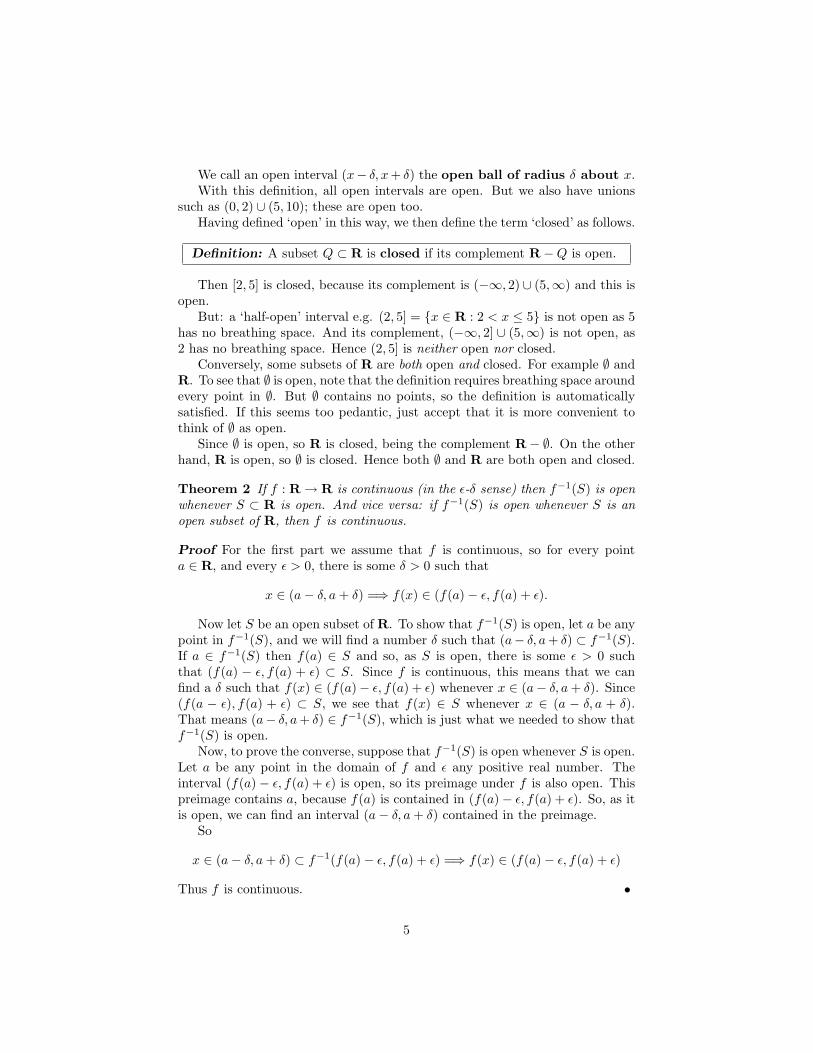
Theorem 2 If f : R→ R is continuous (in the ε-δ sense) then f−1(S) is openwhenever S ⊂ R is open. And vice versa: if f−1(S) is open whenever S is anopen subset of R, then f is continuous.

Proof For the first part we assume that f is continuous, so for every pointa ∈ R, and every ε > 0, there is some δ > 0 such that

x ∈ (a− δ, a + δ) =⇒ f(x) ∈ (f(a)− ε, f(a) + ε).

Now let S be an open subset of R. To show that f−1(S) is open, let a be anypoint in f−1(S), and we will find a number δ such that (a− δ, a + δ) ⊂ f−1(S).If a ∈ f−1(S) then f(a) ∈ S and so, as S is open, there is some ε > 0 suchthat (f(a) − ε, f(a) + ε) ⊂ S. Since f is continuous, this means that we canfind a δ such that f(x) ∈ (f(a)− ε, f(a) + ε) whenever x ∈ (a− δ, a + δ). Since(f(a − ε), f(a) + ε) ⊂ S, we see that f(x) ∈ S whenever x ∈ (a − δ, a + δ).That means (a− δ, a + δ) ∈ f−1(S), which is just what we needed to show thatf−1(S) is open.

Now, to prove the converse, suppose that f−1(S) is open whenever S is open.Let a be any point in the domain of f and ε any positive real number. Theinterval (f(a)− ε, f(a) + ε) is open, so its preimage under f is also open. Thispreimage contains a, because f(a) is contained in (f(a)− ε, f(a) + ε). So, as itis open, we can find an interval (a− δ, a + δ) contained in the preimage.

So

x ∈ (a− δ, a + δ) ⊂ f−1(f(a)− ε, f(a) + ε) =⇒ f(x) ∈ (f(a)− ε, f(a) + ε)

Thus f is continuous. •

5

So we can tell if a function R → R is continuous or not by looking at thepreimages of the open sets. (The term preimage always refers to a function.When the function is not mentioned explicitly, it is assumed that the contextmakes clear what function we are talking about).

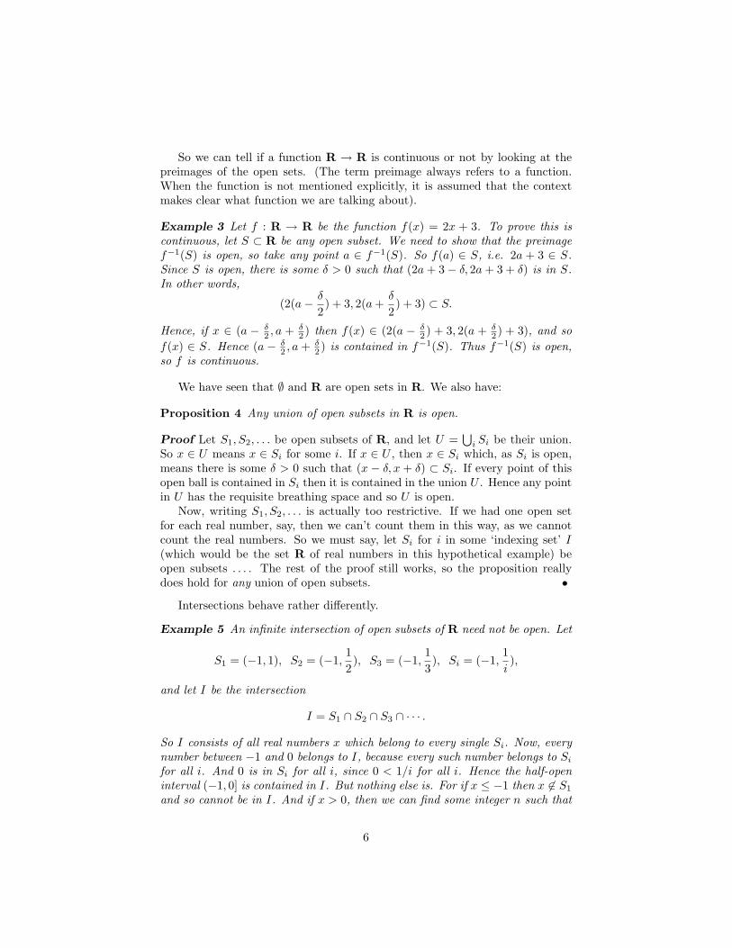
Example 3 Let f : R → R be the function f(x) = 2x + 3. To prove this iscontinuous, let S ⊂ R be any open subset. We need to show that the preimagef−1(S) is open, so take any point a ∈ f−1(S). So f(a) ∈ S, i.e. 2a + 3 ∈ S.Since S is open, there is some δ > 0 such that (2a + 3− δ, 2a + 3 + δ) is in S.In other words,

(2(a− δ

2) + 3, 2(a +

δ

2) + 3) ⊂ S.

Hence, if x ∈ (a − δ2 , a + δ

2 ) then f(x) ∈ (2(a − δ2 ) + 3, 2(a + δ

2 ) + 3), and sof(x) ∈ S. Hence (a − δ

2 , a + δ2 ) is contained in f−1(S). Thus f−1(S) is open,

so f is continuous.

We have seen that ∅ and R are open sets in R. We also have:

Proposition 4 Any union of open subsets in R is open.

Proof Let S1, S2, . . . be open subsets of R, and let U =⋃

i Si be their union.So x ∈ U means x ∈ Si for some i. If x ∈ U , then x ∈ Si which, as Si is open,means there is some δ > 0 such that (x − δ, x + δ) ⊂ Si. If every point of thisopen ball is contained in Si then it is contained in the union U . Hence any pointin U has the requisite breathing space and so U is open.

Now, writing S1, S2, . . . is actually too restrictive. If we had one open setfor each real number, say, then we can’t count them in this way, as we cannotcount the real numbers. So we must say, let Si for i in some ‘indexing set’ I(which would be the set R of real numbers in this hypothetical example) beopen subsets . . . . The rest of the proof still works, so the proposition reallydoes hold for any union of open subsets. •

Intersections behave rather differently.

Example 5 An infinite intersection of open subsets of R need not be open. Let

S1 = (−1, 1), S2 = (−1,12), S3 = (−1,

13), Si = (−1,

1i),

and let I be the intersection

I = S1 ∩ S2 ∩ S3 ∩ · · · .

So I consists of all real numbers x which belong to every single Si. Now, everynumber between −1 and 0 belongs to I, because every such number belongs to Si

for all i. And 0 is in Si for all i, since 0 < 1/i for all i. Hence the half-openinterval (−1, 0] is contained in I. But nothing else is. For if x ≤ −1 then x 6∈ S1

and so cannot be in I. And if x > 0, then we can find some integer n such that

6

x > 1n . (Write x as a decimal, e.g. x = 0.00 · · · 003 · · ·. This is bigger than

0.00 · · · 001 = 1/10k where k is the number of 0s between the decimal point andthe 1.) Hence x 6∈ Sn. Since x does not belong to all of the Sis, x does notbelong to I.

But I = (−1, 0] is not open: the point 0 is contained in I, but every intervalcentred on 0 contains a point bigger than 0 and so outside I.

So not all intersections of open subsets are open. However, things are okayif we take finite intersections.

Proposition 6 A finite intersection of open subsets of R is open.

Proof Let S1, . . . , Sn be open subsets of R and let I be their intersection. Ifx ∈ I then x ∈ S1, x ∈ S2 and so on. Since S1 is open and x ∈ S1, there is someinterval centred on x, contained in S1. Let (x− δ1, x + δ1) be such an interval.Similarly, there is an interval centred on x contained in S2. Let (x− δ2, x + δ2)be such an interval. Carrying on in this way, we get intervals (x− δi, x + δi) foreach i up to n. Let d be the minimum

d = min(δ1, δ2, . . . , δn).

Since there are a finite number of δs here, and all are positive, so d is positive.And since d ≤ δi for all i, we see that (x−d, x+d) is contained in (x−δi, x+δi)for all i. Hence (x− d, x + d) is contained in Si for all i, and so (x− d, x + d) iscontained in I.

Hence, for every point in I, we have constructed an interval, centred on x,contained in I. Thus I is open. •

So we have the following facts about open sets in R:

1. The whole real line is open

2. The empty set is open

3. Arbitrary unions of open sets are open

4. Finite intersections of open sets are open

7

2 Topology

So we can formulate continuity purely in terms of open sets, banishing those εsand δs completely. That is the basis of topology, but we would like to apply itto more than just functions on the real line. In order to define continuity forfunctions between any sets, we have seen that we only need to know what the‘open sets’ are. To ensure that the definition is reasonably sensible, we insistthat they satisfy the same four properties we listed above.

Definition: A topological space X is a set, together with a list, T , ofsubsets of X, called ‘open’ sets, which satisfy the following rules:

T1. The set X itself is ‘open’

T2. The empty set is ‘open’

T3. Arbitrary unions of ‘open’ sets are ‘open’

T4. Finite intersections of ‘open’ sets are ‘open’

The collection T is called the topology on X.

Example 7 The basic example is R, with the sets that we defined above to beopen. We have already noted that they satisfy these four properties. So R,together with these sets, is a topological space.

Example 8 If B is the set {0, 1} consisting of just two elements, then we canmake this a topological space in a couple of different ways.

Firstly, we could agree that only the empty set ∅ and the whole set {0, 1} areto be called open. This satisfies axioms T1 and T2. T3 is also satisfied becausethe only possible union of open sets is where we take ∅ ∪ {0, 1} and the resulthere is {0, 1} which, we have agreed, is open. Finally, T4 is also true, for theonly intersection is ∅ ∩ {0, 1} which is ∅ which, we’ve agreed, is open.

With this topology, the closed sets of {0, 1} would just be the empty set ∅ andthe whole set {0, 1}. Nothing else has a complement which is open, so these arethe only closed sets. The remaining subsets {0} and {1} are neither open norclosed.

Example 9 On the other hand, we can make B a topological space in a differentway, by letting all the subsets ∅, {0}, {1}, {0, 1} be called open. The axioms arethen satisfied, because the empty set and the whole set are included in our listof empty sets, and any intersections or unions will be open since all subsets areopen. Since every subset is open, so every subset is closed as the complement ofany subset will again be a subset and hence open.

Example 10 In fact, given any set S, there are at least two ways of makingS a topological space, illustrated by the preceding examples. On the one hand,we can call only the empty set and S itself open. This is called the indiscretetopology on the set S.

8

And we can take all the subsets of S to be open. This gives the discretetopology. A set with the discrete topology is called a discrete space.

In a topological space X, a subset Q ⊂ X is said to be closed if its comple-ment X −Q is open, i.e. X −Q belongs to the topology on X. For example, inthe indiscrete version of {0, 1}, the only closed subsets are {0, 1} and ∅, whilein the discrete version of {0, 1}, all subsets are closed.

The whole point of defining the term ‘topological space’ was to enable us tomake the following definition.

Definition: A function f : S → T between two topological spaces is con-tinuous if the preimage f−1(Q) of every open set Q ⊂ T is an open subsetof S.

We often write map instead of ‘continuous function’.

Example 11 Let B = {0, 1} with the discrete topology and define f : B → Rby f(0) = −1, f(1) = 1. To check whether or not f is continuous, let U be anyopen set of R. Then

f−1(U) =

{0} if −1 ∈ U and 1 6∈ U{1} if −1 6∈ U and 1 ∈ U{0, 1} if −1 ∈ U and 1 ∈ U∅ if −1 6∈ U and 1 6∈ U.

In each case, the preimage is a subset of B and, since B is discrete, it is open.Hence every preimage of an open set is open, i.e. f is continuous.

Example 12 Now let I = {0, 1} with the indiscrete topology, and B be as above,and define g : I → D by g(0) = 1, g(1) = 0. Then to check whether or not g iscontinuous, we need to look at all the open sets in D. These are: ∅, {0}, {1},{0, 1}. Their preimages are:

g−1(∅) = ∅, g−1{0} = {1}, g−1{1} = {0}, g−1{0, 1} = {0, 1}.

In the first and last case, the preimage is open. But, as I is indiscrete, thesubsets {0} and {1} are not open, so the preimages g−1{1} and g−1{0} are notopen. Since there are open setes in D whose preimages in I are not open, g isnot continuous.

Since continuity is defined in terms of open sets, if we change the topology(i.e. the list of open sets) then we change the notion of continuity. The followingProposition tells us something about the notion of continuity for the discreteand indiscrete topologies.

Proposition 13 If S has the discrete topology and T is any topological space,then any function f : S → T is continuous.

If S has the indiscrete topology and T is any topological space, then anyfunction f : T → S is continuous.

9

Proof If f : S → T is to be continuous, the preimage of any open set must beopen. But if S has the discrete topology, then every subset of S is open, so inparticular, every preimage of an open set must be open. Thus f is continuous.

If f : T → S is to be continuous where S has the indiscrete topology, thenthe preimage of any open set in S must be open in T . But the only open setsin S are the empty set and the whole set S. The preimage of ∅ ⊂ S is ∅ ⊂ T ,which is open. And the preimage of S ⊂ S is the whole of T , which is also open.•

Nevertheless, whatever topologies we use, composites of continuous mapsare always continuous.

Proposition 14 If R,S, T are topological spaces and f : R → S, g : S → Tare continuous functions, then g ◦ f : R→ T is continuous.

Proof Let U ⊂ T be an open set. As g is continuous, g−1(U) is open andhence, as f is continuous, f−1(g−1(U)) is an open set in R. Now (g ◦f)−1(U) =f−1(g−1(U)) since

(g ◦ f)−1(U) = {r ∈ R : g ◦ f(r) ∈ U} = {r ∈ R : g(f(r) ∈ U}= {r ∈ R : f(r) ∈ g−1(U)} = f−1(g−1(U))

Hence (g ◦ f)−1(U) is open whenever U is, i.e. g ◦ f is continuous. •

So, a topological space is a set of points, together with a list of open sets.This is not an easy thing to imagine, as the list of open sets will usually be very,very long.

Another way to think of the topology (the list of open sets) is as the gluewhich sticks the points together. If you take away the topology, then the pointsare like dust and will fall to the floor leaving no trace of how they were joinedtogether. The topology is what explains how things are glued together.

2.1 More Examples of Topological Spaces

In order to construct more interesting examples of topological spaces, we needto be able to use higher dimensions. We can topologize R2 as follows.

Example 15 We put a topology on R2 in a similar way to R. For any point(x, y) in R2 and real number δ > 0, let

Bδ(x, y) = {(x′, y′) ∈ R2 :√

(x′ − x)2 + (y′ − y)2 < δ}.

We call this the open ball of radius δ around (x, y); it is analogous to the openinterval (x − δ, x + δ) in R. A subset of Q ⊂ R2 is defined to be open if, forevery (x, y) ∈ Q, there is some δ > 0 such that Bδ(x, y) is contained in Q.

The proof that this topology satisfies the axioms is much the same as for R.

To give some evidence that this is the ‘right’ topology, we will look at somefamiliar maps from R2 to R.

10

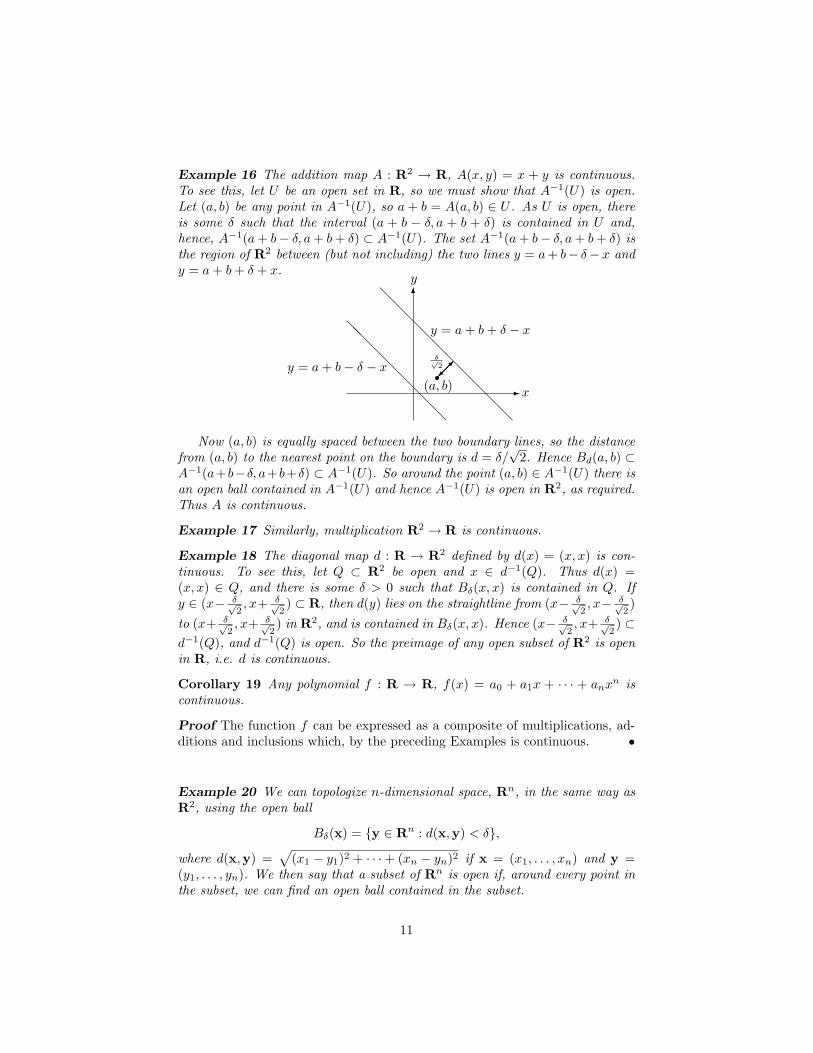
Example 16 The addition map A : R2 → R, A(x, y) = x + y is continuous.To see this, let U be an open set in R, so we must show that A−1(U) is open.Let (a, b) be any point in A−1(U), so a + b = A(a, b) ∈ U . As U is open, thereis some δ such that the interval (a + b − δ, a + b + δ) is contained in U and,hence, A−1(a + b− δ, a + b + δ) ⊂ A−1(U). The set A−1(a + b− δ, a + b + δ) isthe region of R2 between (but not including) the two lines y = a + b− δ−x andy = a + b + δ + x.

-

6

x

y

@@

@@

@@

@@

@@

@@

@@

@@

@@

y = a + b− δ − x

y = a + b + δ − x

•(a, b)

�����

δ√2

Now (a, b) is equally spaced between the two boundary lines, so the distancefrom (a, b) to the nearest point on the boundary is d = δ/

√2. Hence Bd(a, b) ⊂

A−1(a+b−δ, a+b+δ) ⊂ A−1(U). So around the point (a, b) ∈ A−1(U) there isan open ball contained in A−1(U) and hence A−1(U) is open in R2, as required.Thus A is continuous.

Example 17 Similarly, multiplication R2 → R is continuous.

Example 18 The diagonal map d : R → R2 defined by d(x) = (x, x) is con-tinuous. To see this, let Q ⊂ R2 be open and x ∈ d−1(Q). Thus d(x) =(x, x) ∈ Q, and there is some δ > 0 such that Bδ(x, x) is contained in Q. Ify ∈ (x− δ√

2, x+ δ√

2) ⊂ R, then d(y) lies on the straightline from (x− δ√

2, x− δ√

2)

to (x+ δ√2, x+ δ√

2) in R2, and is contained in Bδ(x, x). Hence (x− δ√

2, x+ δ√

2) ⊂

d−1(Q), and d−1(Q) is open. So the preimage of any open subset of R2 is openin R, i.e. d is continuous.

Corollary 19 Any polynomial f : R → R, f(x) = a0 + a1x + · · · + anxn iscontinuous.

Proof The function f can be expressed as a composite of multiplications, ad-ditions and inclusions which, by the preceding Examples is continuous. •

Example 20 We can topologize n-dimensional space, Rn, in the same way asR2, using the open ball

Bδ(x) = {y ∈ Rn : d(x,y) < δ},

where d(x,y) =√

(x1 − y1)2 + · · ·+ (xn − yn)2 if x = (x1, . . . , xn) and y =(y1, . . . , yn). We then say that a subset of Rn is open if, around every point inthe subset, we can find an open ball contained in the subset.

11

Notice how we have put a topology on Rn using only the concept of distancebetween two points. We can do the same in any set which has a reasonable notionof distance; such sets are called metric spaces. This is one way of generatingexamples of topological spaces. Another is by topologizing subsets of knowntopological spaces.

If T is any topological space (for example, Rn), and S ⊂ T is any subset ofT , then the subspace topology on S is defined as follows: A subset of S issaid to be open (in the subspace topology) if it is the intersection of S with anopen set in T . We then refer to S as a subspace of T .

Example 21 Let Z denote the set of integers, a subset of R. If we topologizeZ by the subspace topology, then every set is open. For if n ∈ Z, then {n} =Z ∩ (n− 1

2 , n + 12 ), the intersection of Z with an open set of R. So {n} is open

in Z and, since any union of open sets if open, so any subset of Z is open. Inother words, the subspace topology on Z is the same as the discrete topology.So we say that Z is a discrete space. Proposition 13 then tells us that everyfunction whose domain is Z is continuous.

Example 22 Let S1 be the subset of R2 consisting of all points on the circleof radius 1 around the origin, i.e.

S1 = {(x, y) ∈ R2 : x2 + y2 = 1},

with the subspace topology. This says that a subset of S1 is open if it is theintersection of S1 with an open set in R2. So, for example, one open set in R2

is the open ball B1(1, 1) and hence one open set in S1 will be the intersection S1∩B1(1, 1) which is the quarter-circle between 12 o’clock and 3 o’clock, excludingthe end points (12 and 3 o’clock).

The circle S1 and one of its open sets

Example 23 The 2-sphere S2 is the analogous subset of R3,

S2 = {(x, y, z) ∈ R3 : x2 + y2 + z2 = 1},

with the subspace topology.

12

Example 24 Similarly, we can take the subset consisting of all points of length1 in Rn+1, with the subspace topology. We call this space the n-sphere, denotedby Sn.

We can even allow n = 0: S0 is the set of all points of length 1 in R, so S0

consists of just two points {+1,−1}.The reason we write Sn, rather than Sn+1, for the sphere in Rn+1 is because,

locally, Sn looks like Rn. For example, near the North pole, the circle S1 looksjust like a line, and S2 looks just like a plane.

Example 25 Another useful subset of R2 is the set of non-zero points, R2 −{0}, sometimes written C×, as it corresponds to the set of invertible complexnumbers. We can think of R2−{0} as a topological space by using the subspacetopology.

Similarly, we can take Rn−{0} for any n, and topologize this as a subspaceof Rn.

The subspace topology sometimes gives rise to unexpected open sets.

Example 26 Let [0, 1] be the closed interval in R. With the subspace topologywe can view [0, 1] as a topological space in its own right. Then any interval (a, b)with 0 ≤ a < b ≤ 1 is open, but also an interval [0, b) with b ≤ 1 is open asa subset of [0, 1], since [0, b) is the intersection [0, 1] ∩ (−1, b) of [0, 1] with theopen interval (−1, b) ⊂ R. Similarly, any interval (a, 1] = [0, 1]∩ (a, 2) is open.And, of course, [0, 1] is open too.

So we need to be careful which topological space we are considering whenwe say that a certain set is open.

Example 27 If we take a ring-shaped subset of R3, and define T 2 to be the setof all points on its boundary, with the subspace topology then we get a torus.

To be precise, we can describe the torus T 2 as the set of points (x, y, z) in R3

which satisfyx2 + y2 + z2 − 4

√(x2 + y2) = −3.

Example 28 Now suppose we take a torus, but slice off one side. Put another,matching, sliced torus next to it, so that the two sliced holes face each other.Then if we bring these two sliced tori together until the holes touch, we will geta tubular figure of eight. The resulting topological space is called a surface ofgenus two, which is a fancy way of saying that it has two holes.

13

Example 29 We can form a cylinder by taking all points (x, y, z) in R3 sat-isfying

x2 + y2 = 1 and 0 ≤ z ≤ 1.

Example 30 Now if we cut the cylinder along the line x = −1, y = 0, and givethe resulting ribbon a half twist, then we can stick the ends back together andget a Mobius band. This is famous for only having one side.

Cutting and pasting a subset of R3 in this way does not necessarily giveanother subset of R3. However, in this case it does, and we can topologize theMobius band as the following subset of R3:

M = {(−(3+t sin θ) cos(2θ), (3+t sin θ) sin(2θ), t cos θ) : 0 ≤ θ ≤ π,−1 ≤ t ≤ 1}.

Example 31 The set of all invertible 3 × 3 real matrices forms a set calledGL(3,R) the general linear group. Using the 9 entries in such a matrix asco-ordinates, we can think of GL(3,R) as a subset of R9, and use the subspacetopology to make GL(3,R) into a topological space.

Example 32 Within GL(3,R) there is the subset O(3) of orthogonal matrices,i.e. those matrices P satisfying PT P = I. This subset can again be topologized

14

using the subspace topolgy. The set O(3) is known as the orthogonal group.This is the set of all angle-preserving linear transformations R3 → R3, i.e. allrotations and reflections.

Example 33 Pursuing this line of thought further, if P is an orthogonal matrix,then

det(P )2 = det(PT ) det(P ) = det(PT P ) = det(I) = 1

so det(P ) is either +1 or −1. The subset of 3 × 3 orthogonal matrices ofdeterminant +1 is important, and is called SO(3), the special orthogonalgroup. This is the set of all orientation-preserving, angle-preserving lineartransformations of R3, i.e. rotations.

Example 34 A very interesting space is the set of all straight lines throughthe origin in R3, which we write RP 2 for. This is called the real projectiveplane. It is not a subset of R3, since the elements of RP 2 are not points inR3 but subsets of R3. So we cannot use the subspace topology to make it into atopological space.

Instead, we could topologize it as follows. If we take a subset of RP 2, i.e.a collection of lines in R3, then we can take the union of these lines to geta subset of R3. We could then define the subset of RP 2 to be open if thecorresponding subset of R3 is open, i.e. S ⊂ RP 2 is open if

⋃l∈S l ⊂ R3 is

open. Unfortunately, this gives the indiscrete topology on RP 2, since the unionwill contain 0, unless S is empty, but will not contain an open ball around 0,unless S = RP 2.

To avoid this problem, we omit 0, and we say that a subset S ⊂ RP 2 is openif the subset

⋃l∈S(l− 0) of R3−{0} is open. The empty subset of RP 2 is then

open, because the corresponding subset of R3 − {0} is also the empty set. Andthe wholse set RP 2 is open, because this corresponds to the whole set R3−{0}.

Unions and intersections of subsets of RP 2 correspond to unions and inter-sections of subsets of R3 − {0} so, because the open sets in R3 − {0} form atopology, these open sets in RP 2 also form a topology.

We can define RPn similarly, as the set of lines through the origin in Rn+1.

2.2 Continuity in the Subspace Topology

As we have seen, the topology determines which maps are continuous. So if thesubspace topology is to be useful, we had better check that it gives a sensiblenotion of continuity. This is expressed by the following result.

Proposition 35 (Restriction Theorem) Let S and T be topological spacesand f : S → T a continuous function. Suppose that Q ⊂ S is a subset whoseimage, under f , is contained in a subset R ⊂ T , so that f can be restricted toa function f |Q : Q→ R. If Q and R are given the subspace topologies then f |Qis continuous.

Sf−→ T

∪ ∪Q −→ R

f |Q

15

Proof Let P ⊂ R be an open set in the subspace topology. Then f |−1Q (P ) =

Q ∩ f−1(P ). As P is open in the subspace topology, there must be an open setU ⊂ T such that P = R ∩ U , in which case

f−1(P ) = f−1(R ∩ U) = f−1(R) ∩ f−1(U),

sof |−1

Q (P ) = Q ∩ f−1(R) ∩ f−1(U) = Q ∩ f−1(U)

since Q ⊂ f−1(R) (by assumption: the image of Q under f is contained inR). Now, as f is continuous, and U is open, f−1(U) must also be open. Sof |−1

Q (P ) = Q∩f−1(U) is an open set in the subspace topology on Q. Hence thepreimage under f |Q of any open set in R is open, i.e. f |Q is continuous. •

In other words, if a function on, say S2, is just a restriction of a functiondefined on R3, then the function on S2 will be continuous if the function on R3

is continuous.

Example 36 The inclusion map S2 ↪→ R3 is continuous, as it is simply arestriction of the identity map (x, y, z) 7→ (x, y, z).

Example 37 The determinant function GL(3,R) → R − {0} is continuous.For the formula for the determinant can be used to define a function R9 → Rwhich is continuous, being a composite of additions and multiplications, bothof which are continuous operations, by Examples 16, 17. Since GL(3,R) is asubspace of R9, and R − {0} is a subspace of R, Proposition 35 shows thatdet : GL(3,R)→ R− {0} is continuous.

2.3 Bases

Proving continuity directly can be quite difficult, which is why it is convenient touse short-cuts such as showing that the function is a composite of two continuousfunctions, or a restriction of a continuous function. An alternative approach isto reduce the number of open sets that we need to look at.

Recall that the definition of open subset of Rn says that around every pointin the subset there is an open ball contained in the subset. So the subset is theunion of all these open balls. In other words, every open subset is a union ofopen balls. We say that the open balls form a ‘basis’1 for the topology on Rn.

Definition: In a topological space T , a collection B of open subsets of T issaid to form a basis for the topology on T if every open subset of T can bewritten as a union of sets in B.

Example 38 The collection of all finite open intervals (a, b) (where a, b ∈ R)form a basis for the topology on R, since every open set contains an open intervalaround each point in it and, hence, is the union of all these open intervals.

1Note that this use of the term ‘basis’ has no connection with the usage of the term ‘basis’in linear algebra

16

Example 39 If the set {1, 2, 3} is given the discrete topology, so that everysubset is open, then the sets {1}, {2}, {3} form a basis for this topology, asevery subset of {1, 2, 3} can be written as a union of some of these basic opensets.

If we have a basis for the range space of a given function, then we need onlycheck the preimages of those basic open sets in order to verify continuity of thefunction, thanks to the following result.

Proposition 40 If f : S → T is a function between two topological spaces Sand T , and T has a basis B, then f is continuous if f−1(B) is open for everyset B in the basis B.

Proof For f to be continuous we need to show that f−1(Q) is open for anyopen set Q ⊂ T . Now, as B is a basis for the topology on T , we can write Q asa union of some sets in B. Then the preimage f−1(Q) of Q is the union of thepreimages of these basic sets. Since the preimage of every set in B is open, sof−1(Q) is a union of open sets, and hence open. Thus f is continuous. •

Example 41 Let f : R → R be the function f(x) = 2x + 3. A basis forthe topology on R is given by the collection of all open intervals (a, b). Sincef is an increasing function, f(x) ∈ (a, b) if, and only if, x ∈ (a−3

2 , b−32 ). So

f−1(a, b) = (a−32 , b−3

2 ) which is open. Hence f is continuous.

Example 42 Let f : R→ R be the function f(x) = x2. Again we use the basisof open intervals (a, b); their preimages are as follows:

f−1(a, b) =

(−√

b,−√

a) ∪ (√

a,√

b) if 0 ≤ a < b

(−√

b,√

b) if a < 0 < b∅ if b ≤ 0

In each of these cases, the preimage is open, hence f is continuous.

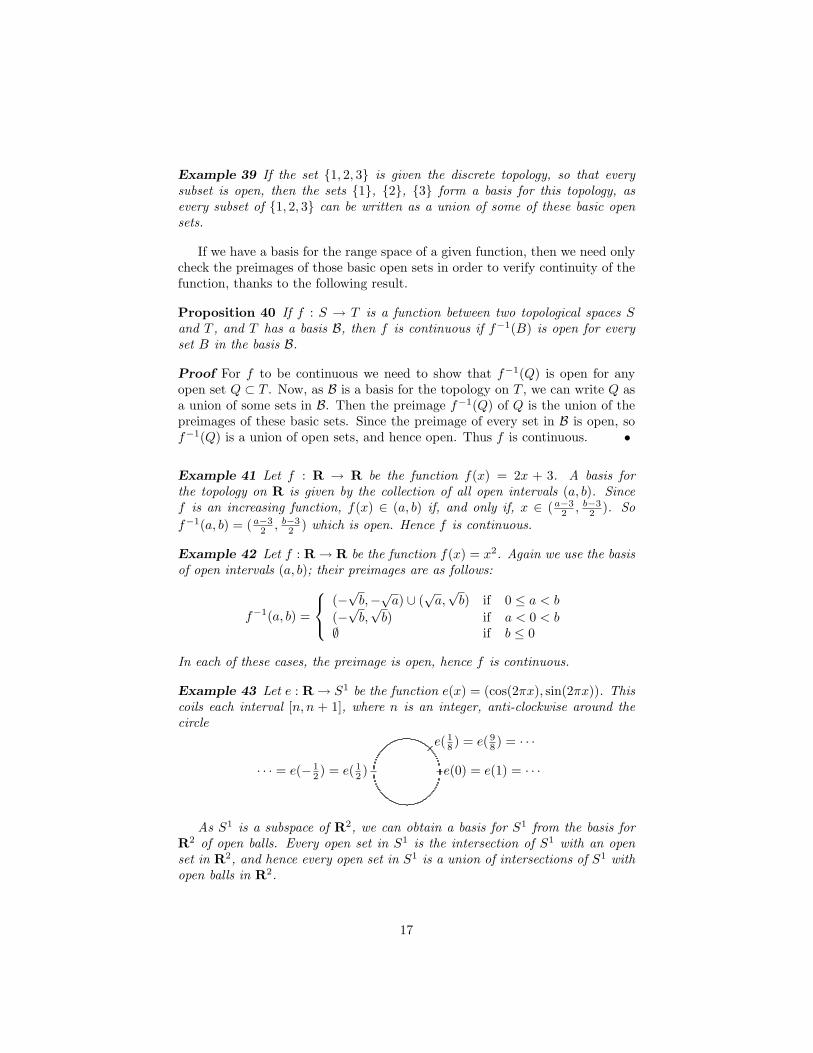
Example 43 Let e : R→ S1 be the function e(x) = (cos(2πx), sin(2πx)). Thiscoils each interval [n, n + 1], where n is an integer, anti-clockwise around thecircle

e( 18 ) = e( 9

8 ) = · · ·

· · · = e(− 12 ) = e( 1

2 ) e(0) = e(1) = · · ·

As S1 is a subspace of R2, we can obtain a basis for S1 from the basis forR2 of open balls. Every open set in S1 is the intersection of S1 with an openset in R2, and hence every open set in S1 is a union of intersections of S1 withopen balls in R2.

17

Most such intersections will be empty and some while give the whole of S1.The preimage of such intersections will either be empty, or the whole of R andhence, in either case, open.

All other intersections will have the form of open arcs, such as S1 ∩B1(1, 1)which was depicted in Example 22. The preimage of this arc is an infinite union

· · · (−2,−74

) ∪ (−1,−34

) ∪ (0,14) ∪ (1,

54) ∪ · · ·

of open intervals, hence it is an open subset of R.Similarly, the preimage of any open arc will be a union of open intervals,

one for each integer, so all such preimages will be open. Hence e is continuous.

18

3 Topological Properties

3.1 Connectivity

A typical example of the type of statement about continuous maps that topol-ogists try to prove is the following.

Theorem 44 There is no continuous surjective map R→ S0.

Proof Suppose that f : R→ S0 is such a map. Since S0 is discrete, the subsets{−1} and {+1} are open and, if f is continuous, then the subsets U = f−1{−1}and V = f−1{+1} of R are open. Since {−1} and {+1} constitute, betweenthem, the whole of S1, so U∪V must be the whole of R. As f is surjective, bothU and V contain at least one point each; they are non-empty. And, because{−1} and {+1} are disjoint, so U ∩ V = ∅. We will see that there can be nosuch open subsets of R.

To do this, let x be any point in U and let y be any point in V . By swappingU and V is necessary, we can assume that x < y. Thus we have an interval[x, y] with one end-point in U and one in V . The mid-point x+y

2 is either in U

or in V . If it is in V , then the interval [x, x+y2 ] has one end-point in U and one

end-point in V . On the other hand, if x+y2 is in U , then the interval [x+y

2 , y]has one end-point in U and one end-point in V . Either way, we can produce aclosed interval of length y−x

2 , with one end-point from each of the sets U andV . Similarly, we can cut this interval in half and, depending on whether themid-point lies in U or in V , we can find an interval of length y−x

4 with oneend-point from each set. Carrying on, we can produce intervals of decreasinglength with one end in either set. The intersection of all of these intervals willbe a single point z of R. If this point lies in U , then there will be an openinterval (z − δz, z + δz) contained in U for some δz > 0. Then any interval oflength < δz containing z will be contained in (z− δz, z + δz) and hence in U . Inparticular, any interval of length y−x

2n will be contained in U if n is large enough(n must be greater than log2(

y−xδz

)). But we know there is such an interval withone end-point in U and one in V . One of these end-points then lies both in Uand V which cannot happen since U ∩V = ∅. Hence z cannot lie in U . Exactlythe same argument can be applied if z lies in V , so we have a contradiction.

The only answer must be that the points x and y cannot have existed, i.e.either U is empty or V is empty. •

This proof relies on the fact that two open subsets of R cannot be disjoint,cover the whole of R and both be non-empty. A space, like R, with this propertyis said to be ‘connected’:

19

Definition: We say that a topological space T is disconnected if it ispossible to find two open subsets U, V of T such that:

• U and V have no intersection, i.e. U ∩ V = ∅

• U and V cover T , i.e. U ∪ V = T

• Neither U nor V are empty, i.e. U 6= ∅ and V 6= ∅.

If there are no such subsets within T , then T is connected.

The first part of the proof of Theorem 44 then tells us the following.

Lemma 45 If T is connected, then there is no continuous surjection T → S0.

Example 46 The space R is connected. The proof of this is the second part ofthe proof of Theorem 44.

Example 47 The open interval (0, 1) is connected. This can be proved in ex-actly the same way as for R. Hence there are no continuous surjective maps(0, 1)→ S0.

Example 48 Similarly, a closed interval such as [0, 1] is connected, as can beseen using the same proof again.

Combining this with Lemma 45 and a little trick yields the Fixed-PointTheorem.

Theorem 49 If f : [0, 1]→ [0, 1] is a continuous map, then f has a fixed point,i.e. there is some x ∈ [0, 1] such that f(x) = x.

Proof Suppose that f : [0, 1]→ [0, 1] is continuous but has no fixed points. Wecan define a map g : [0, 1]→ R by

g(x) =x− f(x)|x− f(x)|

for x ∈ [0, 1]. This is continuous as it is a composite of additions, divisions,and the continuous function f . The value of g(x) is either +1 or −1, so we canrestrict g to a map [0, 1]→ S0 which is continuous by Proposition 35.

Now f(0) ∈ [0, 1] and f(0) 6= 0, so f(0) > 0, i.e. g(0) = −1. Similarly,f(1) < 1 so g(1) = +1. Thus g restricts to a surjective continuous map [0, 1]→S0. By Example 48, [0, 1] is connected, and so no such map can exist. •

Another consequence of Lemma 45 is the following proof of the IntermediateValue Theorem:

Theorem 50 (Intermediate Value Theorem) If f : [a, b]→ R is a contin-uous function and f(a) < 0 and f(b) > 0, then there is some value x ∈ [a, b]such that f(x) = 0.

20

Proof Suppose that there is no such x, i.e. f(x) 6= 0 for all x ∈ [a, b]. Then wecan define a new map f : [a, b]→ S0 by f(x) = f(x)/|f(x)|. This is continuousas f is, and surjective since f(a) < 0 so f(a) = −1, and f(b) > 0 so f(b) = +1.

The interval [a, b] is connected (the argument of Example 48 can easily beadapted to show this) so, by Lemma 45, there can be no such continuous map.Hence our assumption that f(x) 6= 0 for all x ∈ [a, b] must have been incorrect,i.e. there must be some x for which f(x) = 0. •

Lemma 45 also has a converse.

Lemma 51 If T is disconnected, then there is a continuous surjection T → S0.

Proof If T is disconnected, then there are open subsets U, V ⊂ T with U∩V = ∅,U ∪ V = T . We define f : T → S0 as follows. As U and V are disjoint, we candefine f(x) = 1 for x ∈ U and f(x) = −1 for x ∈ V . Since U ∪ V = T , thisdefines f completely, and f is clearly surjective. The preimage of {1} ⊂ S0 isU and the preimage of {−1} ⊂ S0 is V , so both of these are open, hence f iscontinuous. •

This implies the following

Proposition 52 If S is a connected space and T is a disconnected space, thenthere can be no surjective continuous map S → T .

Proof If T is disconnected, then there is a continuous surjection T → S0. Ifthere is also a continuous surjection S → T then we can combine these to get acontinuous surjection S → S0 which cannot happen if S is connected. •

This result can be used both to prove that spaces are continuous and toprove that they are not. For example:

Corollary 53 The circle S1 is connected, because R is connected and the mape : R→ S1 of Example 43 is surjective and continuous.

Corollary 54 The space GL(3,R) is disconnected.

Proof Define a function d : GL(3,R) → S0 by d(M) = det(M)/|det(M)|.Since det is a continuous function, d is continuous. Moreover, d is surjective,since

d

x 0 00 1 00 0 1

= x/|x| ={

1 if x > 0−1 if x < 0.

•

Similarly, the space O(3) is disconnected. The space SO(3), however, isconnected. This is easy to see intuitively, because we no longer have componentsof positive and negative determinant. It is harder to prove rigorously, and wewill leave this until later.

We can also develop the ideas of Theorem 44 in the following way.

21

Lemma 55 If S is a connected space and T is a discrete space, then any con-tinuous map f : S → T is constant.

Proof Let u be a point in the image of f . The set {u} is open as T is discrete.And T − {u}, the set of all points in T other than u, will also be open. Hencef−1({u}) and f−1(T − {u}) will both be open. Moreover, they will be disjoint,since u and T − {u} are disjoint. And they will cover S as {u} ∪ T − {u} = T .Since S is connected, either f−1({u}) or f−1(T − {u}) will be empty. Thepreimage f−1({u}) cannot be empty as it contains u. Hence it must be the casethat f−1(T − {u}) is empty, and f−1{u} = S. This says that the image of f isjust {u}, i.e. f is constant. •

Since R is connected, this implies the following familiar result

Corollary 56 Every continuous map from R to Z is constant.

3.2 Compactness

Another example of a topological fact is that there is no continuous surjection[0, 1] → R. In fact a stronger statement is true, namely that every continuousfunction [0, 1]→ R is ‘bounded’:

Proposition 57 If f : [0, 1] → R is a continuous function then f is bounded,i.e. there are numbers j, k such that Im f ⊂ (j, k). In other words,

j < f(x) < k for all x ∈ [0, 1].

Partial Proof To prove this, suppose that f : [0, 1]→ R is a continuous func-tion. Consider the overlapping open intervals . . . (−2, 0), (−1, 1), (0, 2), (1, 3), . . .in R. These form an open cover of R, meaning that every point in R is con-tained in at least one of these open intervals.

Since f is continuous, the preimage of each interval (i, i+2) is an open subsetof [0, 1]. Every point in [0, 1] must get mapped by f into one of these intervals(i, i + 2) and so must belong to one of the preimages f−1(i, i + 2). Hence thesepreimages f−1(i, i + 2) (taken over all integers i) form an open cover of [0, 1].

If f is bounded, then its image is contained in a finite union of these intervals:if j < f(x) < k for all x, then

Im f ⊂ (j, j + 2) ∪ (j + 1, j + 3) ∪ . . . ∪ (k − 2, k).

Putting this another way, the preimages

f−1(j, j + 2), f−1(j + 1, j + 3), . . . , f−1(k − 2, k)

must cover [0, 1]. So, if f is bounded, then, of our original open cover consistingof all the preimages f−1(i, i + 2), we can discard all but finitely many and stillhave a cover of [0, 1].

22

The converse is also true. If there is a finite number of preimages f−1(i1, i1+2), . . . , f−1(in, in + 2) which cover [0, 1], then the image of f is contained inthe union

(i1, i1 + 2) ∪ (i2, i2 + 2) ∪ . . . ∪ (in, in + 2).

Hence Im f ⊂ (j, k) where j = min(i1, . . . , in), k = max(i1 + 2, . . . , in + 2).So if we can prove that any open cover of [0, 1], such as {f−1(i, i+2), i ∈ Z}

can be ‘refined’ to a finite open cover, then we will be able to deduce that anycontinuous function f : [0, 1]→ R is bounded. •

To complete this proof, then, we need to know that given a certain coveringof [0, 1] by an infinite number of open sets, it is possible to throw away all buta finite number of these open sets and still cover [0, 1]. In other words, we needto know that the infinite open covering of [0, 1] has a ‘finite refinement’.

The open covering of [0, 1] that occurred in the proof was formed by preim-ages f−1(i, i + 2), where i is any integer. These preimages change if we changef , and they can vary greatly. So we need to know that every open cover of [0, 1]has a finite refinement. This property is called ‘compactness’.

Definition: An open covering of a topological space T is a collection ofopen subsets of T such that every point in T lies in at least one of theseopen subsets.A topological space T is said to be compact if every open covering of Tadmits a finite refinement. In other words, given any infinite collection ofopen sets, which covers T , it is possible to throw most of these sets away,keeping only a finite number of them, and still have an open covering of T .

To complete the proof, then, we need to show that the interval [0, 1] iscompact.

Proposition 58 The closed interval [0, 1] is compact.

Proof To prove that [0, 1] is compact, suppose that we have an open cover of[0, 1]. We will show that this open cover has a finite refinement by contradiction,so let us assume that there is no finite refinement of this cover. Now considerthe intervals [0, 1

2 ] and [ 12 , 1]. Intersecting the original open cover with each ofthese intervals gives an open cover for each interval. If they both admit a finiterefinement, then we can combine these to get a finite refinement of the originalopen cover. We have assumed that this is not the case, so one of the intervalsmust not have a finite refinement. Let I1 be this interval.

Now we divide I1 in two halves. The same argument shows that one ofthese two halves must not have a finite refinement; let I2 be that half. We thendivide I2 in half and so on. Carrying on in this way, we obtain a nested seriesof intervals:

[0, 1] ⊃ I1 ⊃ I2 ⊃ · · ·of decreasing length: In has length 1/2n, and none of these intervals admit afinite refinement of the open cover. The intersection of all of these intervals will

23

be a single point c ∈ [0, 1]. This must be contained in one of the sets in theopen cover. Since this set is open, it must also contain some breathing space(c− δc, c + δc) where δc > 0. But this will contain any interval around c if thelength of the interval is less than δc. In particular (c − δc, c + δc) will containIn if n > log2(

1δc

). So, for n large enough, the interval In will be contained in(c − δc, c + δc) which, we noted, was contained in one of the open sets in thecover. However, this contradicts our assumption that none of the intervals In

admitted a finite refinement. Hence that assumption must have been wrong,in which case that original interval [0, 1] must admit a finite refinement of thecover. Thus a closed interval [0, 1] is compact. •

So [0, 1] is compact, and the proof of Proposition 57 is complete. Now,notice that the proof of Proposition 57 didn’t use any information about [0, 1]apart from the fact that it was compact. So the same proof can be used for thefollowing.

Proposition 59 If T is a compact topological space and f : T → R is a con-tinuous function, then f is bounded.

In other words, all spaces which are compact have this property about con-tinuous functions to R. If we can show that any given space is compact, we willbe able to deduce this property about real valued functions on that space.

Lemma 60 The circle S1 is compact.

Proof We will prove this by relating S1 to the interval [0, 1] which we know iscompact. Let f : [0, 1]→ S1 be the map f(t) = (cos(2πt), sin(2πt)) of Example43.

Now, let U be any open cover of S1, so U is a collection of open subsets ofS1. For each subset Q ∈ U , we have an open subset f−1(Q) of [0, 1], as f iscontinuous. The collection of all of these open subsets f−1(Q) for Q ∈ U is anopen cover of [0, 1], and so has a finite refinement. Let V be a finite collectionof open subsets Q taken from U such that ∪Q∈Vf−1(Q) covers [0, 1]. Then V isa finite refinement of U for the circle S1. For if x ∈ S1, then x is in the image off , as f is surjective. Hence there is some y ∈ [0, 1] such that f(y) = x. As [0, 1]is covered by ∪Q∈Vf−1(Q), there must be some Q ∈ V such that y ∈ f−1(Q).If y ∈ f−1(Q) then f(y) ∈ Q, so x ∈ Q. Hence, for each point x in S1, there issome subset in V which contains x. Thus V is a finite refinement of U , and S1

is compact. •

Having proved that, we get the following corollary for nothing.

Corollary 61 Any continuous map from S1 to R is bounded.

Note also that the proof of Proposition 58 can be adapted very easily toshow

Proposition 62 Any closed interval [a, b] ⊂ R is compact.

Of course, many spaces are not compact.

24

Example 63 The space R cannot be compact because not all continuous func-tions from R to R are bounded (for example, the identity function f(x) = x isnot bounded on R).

One open cover of R that does not have a finite refinement is the following.Let Un = (−n, n) for each positive integer n. Every real number belongs to oneof these open intervals, so they form an open cover of R. However, if we take afinite number of these intervals, say Ui1 , Ui2 , . . . , Uik

, then these will not coverR. For their union will simply equal (−i, i) = Ui where i = max(i1, . . . , ik).There are many real numbers which are not contained in Ui, so any such finiterefinement will fail to be an open cover of R. Hence the original, infinite opencover cannot be refined finitely to give an open cover.

Example 64 One can show that the open interval (0, 1) is not compact in asimilar way, defining open sets Un for all integers n > 1 by

U2 = (12, 1), U3 = (

13, 1), . . . , Un = (

1n

, 1), . . . .

These cover (0, 1), because if any real number x is between 0 and 1 then it isalso between 1/n and 1 for some sufficiently large integer n. But if we take anyfinite refinement, say Ui1 , . . . , Uik

then this will not cover (0, 1). For, the unionof such a finite collection will again be Ui where i is the maximum of i1, . . . , ik.And Ui omits some points from (0, 1), such as 1/i. Hence no finite refinementof this cover is itself a cover of (0, 1) and so (0, 1) is not compact.

The proof of Lemma 60 can be very easily generalized to prove the followingresult.

Proposition 65 If f : S → T is a continuous map and S is compact, then theimage of f is compact.

That is to say, the image of a compact space under a continuous map iscompact. This leads immediately to the following fact.

Corollary 66 There is no continuous surjective map [0, 1]→ (0, 1).

Finally, for subspaces of Rn, there is a complete classification of compactspaces, in terms of whether or not the subspace is closed when considered as asubset of Rn, and whether or not it is ‘bounded’. We say that a subset S ofRn is bounded if there is some real numbers d such that S is contained in theopen ball Bd(0) of radius d around the origin.

Theorem 67 (Heine-Borel Theorem) If T is a subspace of Rn, then T iscompact if, and only if, T is closed and bounded.

Proof We will only prove this in the case where n = 1, as the general case isvery similar, but the details tend to obscure the ideas.

First suppose that T is any closed, bounded subset of R, and we will provethat T must be compact. The fact that T is bounded means that T is contained

25

in some open interval (−d, d) for some real number d > 0. In particular, T iscontained within the closed interval [−d, d]. If T is closed, then its complementR−T is open. If we have an open cover of T then, by definition of the subspacetopology, each open set is the intersection of T with an open subset of R. Takingall these open subsets of R together with the open set R−T must give an opencover of R. Intersecting all these open subsets of R (including R − T ) with[−d, d] will then give an open cover of [−d, d].

We have already proven that any closed interval of R is compact, so any opencover of [−d, d] admits a finite refinement. So we can discard all but finitelymany of the open subsets of R and still have a cover of [−d, d] when we intersectwith this interval. If this finite list of open subsets covers [−d, d], then it willcertainly cover T . By intersecting these open subsets of R with T we will havea finite refinement of the original cover of T , since the only extra set we addedwas R−T , and this will vanish when we intersect with T , since R−T ∩T = ∅.Hence T is compact.

Now we will prove the opposite result. We will show that if T is not closed,or if it is not bounded, then it cannot be compact.

Suppose, then, that T is not a closed set of R. So the complement of T isnot open, and therefore has some point x 6∈ T such that no neighbourhood of xis contained in the complement of T . In other words, every interval (x−δ, x+δ),with δ > 0, contains an element of T .

Let In be the intersection of T with the complement of the interval [x −1n , x + 1

n ]. So y ∈ In if y ∈ T and either y < x− 1n or y > x + 1

n .If now y is any element of T , then y 6= x so |y − x| > 0. In particular, we

can find an integer n such that |y − x| > 1/n. Thus y 6∈ [x − 1n , x + 1

n ]. Sincey ∈ T , we see that y ∈ In. Hence the union of the In’s contains every elementof T . So this is an open cover of T .

Now I1 ⊂ I2 ⊂ I3 ⊂ · · · and so any finite union of In’s will be equal to Im,where m is the largest index involved. And Im does not contain [x− 1

m , x+ 1m ].

But every interval (x− 1m , x+ 1

m ) contains a point of T . Hence Im cannot coverT , and so there can be no finite refinement of the In’s which covers T . Thus Tis not compact.

Finally, suppose that T is not bounded. Then let In = (−n, n) for eachinteger n > 0. Every real number x is contained in In for some n. So the In’scover R and, consequently, T .

If we take a finite number of these In’s, then their union will be equal to Im

for some m. If T is not bounded, then for each real number k, there is somex ∈ T such that either x > k or x < −k. In particular, for every integer n > 0,there is some x ∈ T such that x 6∈ In. Hence Im cannot cover T , so T is notcompact. •

3.3 Hausdorff spaces

The last property that we will meet for now is the ‘Hausdorff’ property.

26

Definition: We say that a topological space T is Hausdorff if, for any twodistinct points x, y in T , there are open subsets U, V of T such that x ∈ Uand y ∈ V and U ∩ V = ∅.

In other words, around any two distinct points, we can find two non-overlappingopen sets. The traditional way of saying this is that any two distinct points canbe ‘housed off’ from each other.

••

Example 68 The interval [0, 1] is Hausdorff. To prove this, let x, y ∈ [0, 1]be two distinct points. Then |y − x| > 0, and we can set δ = |y − x|/2. LetU = (x−δ, x+δ)∩ [0, 1] and V = (y−δ, y+δ)∩ [0, 1]. As these are intersectionsof [0, 1] with open sets, they are both open. And x ∈ U , y ∈ V and U ∩ V = ∅,by the way we chose δ.

Example 69 Similarly, Rn is Hausdorff, for any n.

If a space is Hausdorff then we have the following information about self-maps of the space:

Proposition 70 If T is a Hausdorff space and f : T → T is a continuous map,then the fixed point set

Fix(f) = {x ∈ T : f(x) = x}

is a closed subset of T .

Proof To prove that a subset is closed we must prove that its complement isopen. So let y be a point in the complement of Fix(f). Then as y is not a fixedpoint of f , we see that f(y) 6= y. Thus we have two distinct points y, f(y) of T ,so we can find open sets U, V , with y ∈ U , f(y) ∈ V and U ∩ V = ∅. Since f iscontinuous, f−1(V ) is open, and so U ∩f−1(V ) will be an open set containing y.Moreover, U ∩f−1(V ) is disjoint from Fix(f). For suppose that x ∈ U ∩f−1(V )and f(x) = x. If x ∈ U ∩ f−1(V ) then x ∈ f−1(V ) and so f(x) ∈ V . But alsox ∈ U and if f(x) = x then f(x) ∈ U . So we have f(x) ∈ U ∩V , whereas U ∩Vis empty. So U ∩ f−1(V ) is disjoint from Fix(f) as I claimed.

Hence, around every point y in the complement of Fix(f), we can find anopen set containing y and contained in the complement of Fix(f). The union ofall these open sets (one for each point in the complement) will still be open, willbe contained in the complement of Fix(f) and will also cover that complement.Hence the complement is open and Fix(f) is closed. •

Corollary 71 If f : [0, 1] → [0, 1] is a continuous map then the fixed point setfor f is a closed subset of [0, 1]

27

The following result tells us that most spaces that we meet will be Hausdorff:

Proposition 72 If f : S → T is continuous and injective and T is Hausdorff,then S is Hausdorff.

Proof Let x, y ∈ S be two distinct points. As f is injective, f(x) and f(y) in Twill be distinct. Therefore there are open subsets U, V ⊂ T such that f(x) ∈ U ,f(y) ∈ V and U ∩ V = ∅. Since f is continuous, the preimages f−1(U) andf−1(V ) will be open subsets of S. Moreover, x ∈ f−1(U) and y ∈ f−1(V ).Finally, f−1(U) ∩ f−1(V ) = f−1(U ∩ V ) = f−1(∅) = ∅. •

So any subspace of a Hausdorff space is automatically Hausdorff. In partic-ular, all subspaces of Rn are Hausdorff, so almost every space that we have metso far is Hausdorff.

It is harder to think of examples of non-Hausdorff spaces. A simple examplecan be obtained using the indiscrete topology.

Example 73 The set {1, 2}, with the indiscrete topology, is not Hausdorff. Forif we take x = 1 and y = 2, then the only open set containing x is the whole set,which also contains y. Thus it is not possible to find two non-overlapping opensets each containing only one of the points.

A subtler example is the following.

Example 74 Let L be the real line together with an extra point which we’llcall 0′, and think of as an extra 0. We make this into a topological space inthe following way. For every subset of R that does not contain 0, there is acorresponding subset of L, and we define this subset of L to be open if thecorresponding subset of R is open. For each subset of R that contains 0, thereare three corresponding subsets of L: one which contains 0, one which contains0′, and one which contains both. We define all three to be open if the originalsubset of R is open. The open sets on L that this gives do actually form atopology, i.e. they satisfy the axioms T1-T4, as you can check.

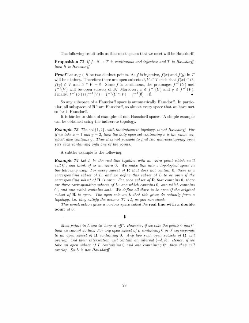
This construction gives a curious space called the real line with a doublepoint at 0:

••

Most points in L can be ‘housed-off’. However, if we take the points 0 and 0′

then we cannot do this. For any open subset of L containing 0 or 0′ correspondsto an open subset of R containing 0. Any two such open subsets of R willoverlap, and their intersection will contain an interval (−δ, δ). Hence, if wetake an open subset of L containing 0 and one containing 0′, then they willoverlap. So L is not Hausdorff.

28

4 Deconstructionist Topology

Typically topologists are presented with a space (or rather, with some descrip-tion of a space) and asked what they can say about it. The obvious, but slow,approach would be to go through their list of topological properties and seewhich ones hold and which ones don’t. But there are many shortcuts.

The most useful trick is that sometimes by a clever piece of insight, a topol-ogist will recognize that an apparently unfamiliar space is actually identical to afamiliar space. If this is the case, then any properties of that more familiar spaceautomatically hold for the unfamiliar one. So for this we need to know what‘identical’ means for topological spaces. This is the concept of ‘homeomorphism’that we will meet in the first section.

It is often the case, however, that the new space is more complicated thanthe ones we know about. Nevertheless, it is often possible to build the new spaceout of familiar spaces. There are many different ways of building new spacesout of old ones. Obviously, the more ways we know, the greater the chances ofbeing able to construct the particular space we wish to study. So later we willlook at a number of different ‘topological constructions’. Keep an eye on whichproperties are preserved by these constructions, and how other properties arechanged, as we want to use these constructions to deduce information about thenew space from information about its constituent pieces.

Some spaces that we meet turn out not to be identical to familiar ones but tobe at least quite similar to them. In other cases, it may be possible to constructa space identical to the one we are interested in via complicated process, butalso possible to build a similar (though not identical) space with a much lesscomplicated process. The most useful notion of ‘similarity’ is that of ‘homotopyequivalence’ which we will study in the last few sections of this chapter. Many ofthe properties that we are interested in are shared by spaces which are homotopyequivalent, but others are not, so we need to be careful about that.

4.1 Homeomorphisms

For two topological spaces to be identical, they should have the same points,and the same topology. The easiest way to say this rigorously is as follows.

Definition: If S and T are two topological spaces, and f : S → T andg : T → S are continuous functions such that

(f ◦ g)(y) = y for all y ∈ T

and(g ◦ f)(x) = x for all x ∈ S

then S and T are said to be homeomorphic and the maps f and g arehomeomorphisms. The maps f and g are inverse to each other, so we maywrite f−1 in place of g and g−1 in place of f . If S and T are homeomorphicthen we write S ∼= T .

29

Example 75 If S and T are actually the same topological space, for exampleS = T = R, then certainly S and T are homeomorphic, for we can take thefunctions f and g to be the identity maps f(x) = x and g(x) = x. These areclearly inverse to each other, and they are both continuous as, for example thepreimage f−1(U), of an open subset U ⊂ T , is just U itself and so open.

Example 76 Any two open intervals of the real line are homeomorphic. Forexample, if S = (−1, 1) and T = (0, 5), then define f : S → T and g : T → S by

f(x) =52(x + 1), g(x) =

25x− 1.

These are both continuous, being composites of addition and multiplication. Andf and g are clearly inverse to each other, so they are homeomorphisms. Hence,by the Proposition, (−1, 1) and (0, 5) are homeomorphic.

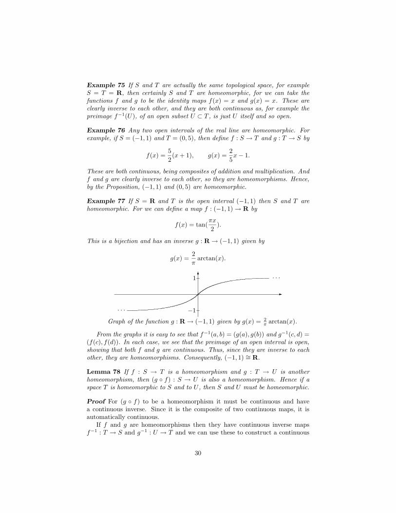
Example 77 If S = R and T is the open interval (−1, 1) then S and T arehomeomorphic. For we can define a map f : (−1, 1)→ R by

f(x) = tan(πx

2).

This is a bijection and has an inverse g : R→ (−1, 1) given by

g(x) =2π

arctan(x).

-

6 . . .

. . . −1

1

Graph of the function g : R→ (−1, 1) given by g(x) = 2π arctan(x).

From the graphs it is easy to see that f−1(a, b) = (g(a), g(b)) and g−1(c, d) =(f(c), f(d)). In each case, we see that the preimage of an open interval is open,showing that both f and g are continuous. Thus, since they are inverse to eachother, they are homeomorphisms. Consequently, (−1, 1) ∼= R.

Lemma 78 If f : S → T is a homeomorphism and g : T → U is anotherhomeomorphism, then (g ◦ f) : S → U is also a homeomorphism. Hence if aspace T is homeomorphic to S and to U , then S and U must be homeomorphic.

Proof For (g ◦ f) to be a homeomorphism it must be continuous and havea continuous inverse. Since it is the composite of two continuous maps, it isautomatically continuous.

If f and g are homeomorphisms then they have continuous inverse mapsf−1 : T → S and g−1 : U → T and we can use these to construct a continuous

30

inverse for (g ◦ f), namely f−1 ◦ g−1. This is again continuous, as it is thecomposite of two continuous maps. And it is an inverse for (g ◦ f) because, ifx ∈ S we have

(f−1 ◦ g−1) ◦ (g ◦ f)(x) = f−1(g−1(g(f(x)) = f−1(f(x)) = x

and similarly (g ◦ f)(f−1 ◦ g−1)(y) = y for y ∈ U . •

Corollary 79 Any open interval of the real line is homeomorphic with R itself.

Proof We have seen that R ∼= (−1, 1) and that any two open intervals arehomeomorphic. In particular, any open interval is homeomorphic with (−1, 1).Hence, by the lemma, any open interval is homeomorphic with R. •

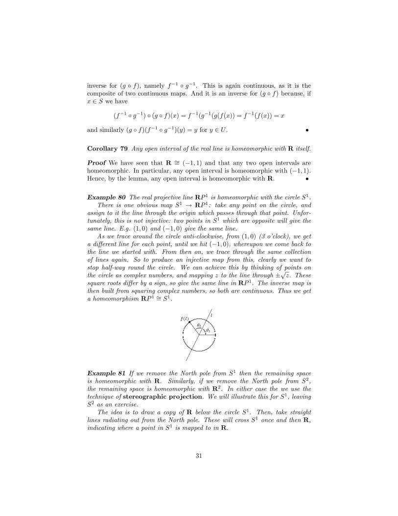
Example 80 The real projective line RP 1 is homeomorphic with the circle S1.There is one obvious map S1 → RP 1: take any point on the circle, and

assign to it the line through the origin which passes through that point. Unfor-tunately, this is not injective: two points in S1 which are opposite will give thesame line. E.g. (1, 0) and (−1, 0) give the same line.

As we trace around the circle anti-clockwise, from (1, 0) (3 o’clock), we geta different line for each point, until we hit (−1, 0), whereupon we come back tothe line we started with. From then on, we trace through the same collectionof lines again. So to produce an injective map from this, clearly we want tostop half-way round the circle. We can achieve this by thinking of points onthe circle as complex numbers, and mapping z to the line through ±

√z. These

square roots differ by a sign, so give the same line in RP 1. The inverse map isthen built from squaring complex numbers, so both are continuous. Thus we geta homeomorphism RP 1 ∼= S1.

��������

SS

•l

f(l)

θl

θl

Example 81 If we remove the North pole from S1 then the remaining spaceis homeomorphic with R. Similarly, if we remove the North pole from S2,the remaining space is homeomorphic with R2. In either case the we use thetechnique of stereographic projection. We will illustrate this for S1, leavingS2 as an exercise.

The idea is to draw a copy of R below the circle S1. Then, take straightlines radiating out from the North pole. These will cross S1 once and then R,indicating where a point in S1 is mapped to in R.

31

-

��� �� AU

@@@R

This construction is also often used when we remove more than just a singlepoint from S1 or S2.

If we take the region of S2 to the South of the equator (or any fixed latitude),then this is homeomorphic to a disc (closed or open according to whether ornot we include the equator) under stereographic projection. So, for example, theSouthern hemisphere, including the equator, is homeomorphic to a closed disc inR2. The part of S2 South of (and excluding) the Arctic circle is homeomorphicto an open disc.

If we give R an extra point, called ∞, then we can extend the homeomor-phism S1−{(0, 1)} ↔ R to a bijection R∪{∞} ↔ S1. We can then put a topol-ogy R∪{∞} in such a way as to make the extended map a homeomorphism. Forexample, an open neighbourhood of∞ would be a union (−∞,−a)∪(a,∞)∪{∞}.

Similarly, we can construct a homeomorphism between S2 and R2∪{∞} (orC ∪ {∞}) with a suitable topology. This model of S2 is called the Riemannsphere.

Example 82 A solid square is homeomorphic to a solid disc. We will illustratethis with the square

Q = {(x, y) ∈ R2 : −1 ≤ x ≤ 1,−1 ≤ y ≤ 1}

and discD = {(x, y) ∈ R2 : x2 + y2 ≤ 1}.

Define f : D → Q by

f(x, y) =

√x2 + y2

max(|x|, |y|)(x, y)

if (x, y) 6= (0, 0) and f(0, 0) = (0, 0). Its inverse g : Q→ D is given by

g(x, y) =max(|x|, |y|)√

x2 + y2(x, y)

if (x, y) 6= (0, 0); g(0, 0) = (0, 0).The idea of these maps is that f pushes the disc out radially to form a square,

and g contracts the square radially to form a disc. Using this idea you can seethat the preimage of an open subset of Q under f will be open in D and similarlyfor g. So they are continuous maps.

��

��@@

@@

j

Y

f

g ��

��

�@@

@@

@

32

Example 83 Similarly, a cube is homeomorphic to a solid ball.

There are many homeomorphisms like this which are easy to see you whenyou get the hang of things. The most celebrated is the following.

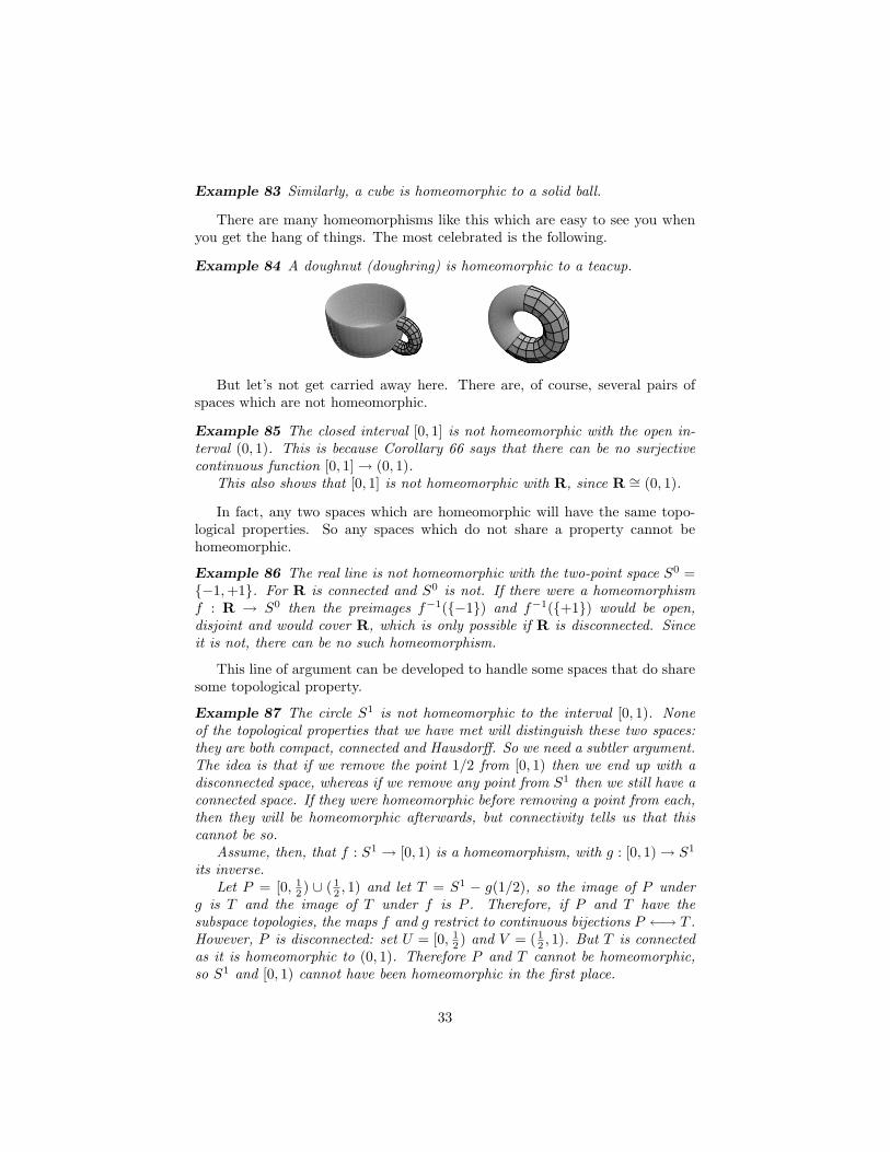
Example 84 A doughnut (doughring) is homeomorphic to a teacup.

But let’s not get carried away here. There are, of course, several pairs ofspaces which are not homeomorphic.

Example 85 The closed interval [0, 1] is not homeomorphic with the open in-terval (0, 1). This is because Corollary 66 says that there can be no surjectivecontinuous function [0, 1]→ (0, 1).

This also shows that [0, 1] is not homeomorphic with R, since R ∼= (0, 1).

In fact, any two spaces which are homeomorphic will have the same topo-logical properties. So any spaces which do not share a property cannot behomeomorphic.

Example 86 The real line is not homeomorphic with the two-point space S0 ={−1,+1}. For R is connected and S0 is not. If there were a homeomorphismf : R → S0 then the preimages f−1({−1}) and f−1({+1}) would be open,disjoint and would cover R, which is only possible if R is disconnected. Sinceit is not, there can be no such homeomorphism.

This line of argument can be developed to handle some spaces that do sharesome topological property.

Example 87 The circle S1 is not homeomorphic to the interval [0, 1). Noneof the topological properties that we have met will distinguish these two spaces:they are both compact, connected and Hausdorff. So we need a subtler argument.The idea is that if we remove the point 1/2 from [0, 1) then we end up with adisconnected space, whereas if we remove any point from S1 then we still have aconnected space. If they were homeomorphic before removing a point from each,then they will be homeomorphic afterwards, but connectivity tells us that thiscannot be so.

Assume, then, that f : S1 → [0, 1) is a homeomorphism, with g : [0, 1)→ S1

its inverse.Let P = [0, 1

2 ) ∪ ( 12 , 1) and let T = S1 − g(1/2), so the image of P under

g is T and the image of T under f is P . Therefore, if P and T have thesubspace topologies, the maps f and g restrict to continuous bijections P ←→ T .However, P is disconnected: set U = [0, 1

2 ) and V = (12 , 1). But T is connected

as it is homeomorphic to (0, 1). Therefore P and T cannot be homeomorphic,so S1 and [0, 1) cannot have been homeomorphic in the first place.

33

You can see that it is much easier to show that two spaces are not homeomor-phic if there is some simple property (such as connectedness or compactness)which is not shared by both spaces. This is one reason for studying as manysuch properties as possible.

There is one subtlety about homeomorphisms that I must warn you about.We agreed that a map f : S → T is a homeomorphism if it is continuous and hasa continuous inverse g : T → S. This, of course, implies that f is a bijection.But

A continuous bijection is not always a homeomorphism.

Example 88 Let S = {1, 2} with the discrete topology and let T = {1, 2} withthe indiscrete topology. Let f : S → T be the identity function, then f isbijective, and continuous since any function from a discrete space is continuous.However, the inverse map g : T → S is not continuous. For {1} is open in thediscrete space S, but g−1{1} = {1} is not open in T .

A more complicated, but more interesting example is the following.

Example 89 Let f : [0, 1)→ S1 be the restriction of the map e of Example 43,so

f(t) = (cos(2πt), sin(2πt)).

As e is continuous, so is f , and it is clear that f is a bijection. But f can-not be a homeomorphism because we have just seen that [0, 1) and S1 are nothomeomorphic. The problem is that f−1 is not continuous.

Since f is bijective, there is no choice in the definition of its inverse map:f−1 must send (cos(2πt), sin(2πt)) to t ∈ [0, 1). However, the half-open interval[0, 1

2 ) is an open subset of [0, 1) in the subspace topology, and its preimage underthis inverse map f−1 will be the half-open interval of all points between 9 o’clockand 3 o’clock, including 3 o’clock but excluding 9 o’clock. This preimage is notan open subset of S1, as it has no breathing space around 3 o’clock.

Having said that, we can use the properties of compactness and Hausdorff-ness to avoid such behaviour.

Theorem 90 If X is a compact space, Y is a Hausdorff space and f : X → Yis a continuous function which is bijective, then there is a continuous inversefunction g : Y → X with gf = 1X and fg = 1Y . Hence f is a homeomorphism.

We will prove this using three lemmas.

Lemma 91 If X is compact and U ⊂ X is a closed subspace, then U is compact.

Proof As U is closed, its complement X−U is open. Therefore any open coverof U can be made into an open cover of X by including the open set X −U . AsX is compact, this cover of X may be finitely refined and, by omitting X − U ,we will obtain a refinement of the open cover of U . •

34

Lemma 92 If Y is Hausdorff and V ⊂ Y is compact, then V is closed.

Proof Let u be any point in the complement Y − V . For each point v ∈ V ,we have v 6= u, so there are disjoint open sets Uu,v containing u and Xu,v

containing v. Since Xu,v contains v, we can obtain an open cover of V bytaking {V ∩ Xu,v : v ∈ V }. As V is compact, this cover can be refined to afinite collection of open sets. Taking the intersection of the corresponding opensets Uu,v gives an open set (since finite intersections of open sets are open) Uu

which is disjoint from each open set Xu,v. Consequently, Uu is disjoint from V ,since every point of V lies in some set Xu,v. In other words, Uu is containedin Y − V . Thus, for every point u ∈ Y − V , we have constructed an open setcontained in Y − V and containing the point u. So Y − V is the union of allthese open sets and, hence, is open. So V is closed. •

Lemma 93 Let f : S → T be a function between two topological spaces. Thenf is continuous if, and only if, f−1(C) is closed whenever C ⊂ T is closed.

Proof If f is continuous and C is closed, then T −C is open, so f−1(T −C) isopen, so f−1(C) = S − f−1(T − C) is closed.

If f−1(C) is closed whenever C is, and U ⊂ T is an open set, then T − U isclosed, so f−1(T − U) is closed and, hence f−1(U) = S − f−1(T − U) is open.•

Proof of Theorem 90 Let f : X → Y be a continuous bijection. As it is abijection, there is an inverse function g : Y → X and we must show that g iscontinuous. We will do this using Lemma 93, so suppose that U ⊂ X is closed.By Lemma 91, U is compact, as X is compact. Then g−1(U) is the image ofU under the continuous map f , so g−1(U) is compact by Proposition 65. Nowg−1(U) is a compact subset of a Hausdorff space Y so, by Lemma 92, g−1(U)is closed. Thus g is continuous. •

4.2 Disjoint unions

Having established what we mean by saying two topological spaces are ‘thesame’, we now turn to ways of building new topological spaces out of old ones.The simplest such construction is that of forming ‘disjoint unions’.

Example 94 The space S0 = {−1,+1} is the disjoint union of two one-pointspaces {−1} and {+1}:

S0 = {−1} q {+1}.

If we have any two topological spaces S, T then we can define their disjointunion S q T as follows. The points in S q T are all the points of S togetherwith all the points in T . A subset Q of SqT is open if Q∩S is open and Q∩Tis open. So the open sets of S q T are just the unions of an open set in S withan open set in T .

35

Example 95 We can form a set of train tracks by taking RqR:

One open set is (0, 4)q (10, 16):

( )( )

0 4

10 16Another is ∅ q (3, 8):

( )3 8

Note that if S and T are both subsets of a given space and S ∩ T is notempty, then in S q T we count the points in the intersection twice. This isillustrated by the following example.

Example 96 The disjoint union of the circle S1 and the interval [−2, 2] ishomeomorphic to a ‘rising sun’

and not homeomorphic to an ‘underground sign’

Note that every (non-trivial) disjoint union is disconnected, for S and T areopen subsets of S q T and S ∩ T = ∅ and S ∪ T = S q T . (I am assuming thatboth S and T are non-empty). And conversely every disconnected space is adisjoint union.

Example 97 The punctured real line R − {0} = (−∞, 0) ∪ (0,∞) can be ex-pressed as a disjoint union (−∞, 0)q (0,∞) ∼= R qR, since any open intervalis homeomorphic with R.

The disjoint union construction is very useful for our deconstructive purposesas it carries a lot of topological information. For example, we can describecontinuous maps to or from a disjoint union very precisely in terms of maps toor from the separate components.

Theorem 98 If Q is a connected topological space then a continuous map Q→S q T corresponds to either a continuous map Q → S or a continuous mapQ→ T .

If R is any topological space then a continuous map S q T → R correspondsto a pair of continuous maps (S → R, T → R).

36

Proof If f : Q→ S q T is continuous, then the preimages f−1(S) and f−1(T )will both be open. Their union is f−1(S q T ) = Q, and their intersectionis empty. So as Q is connected, either f−1(S) or f−1(T ) must be empty. Iff−1(S) = ∅, then the image of f is contained in T , so we can think of f as acontinuous map Q→ T . If, on the other hand, f−1(T ) = ∅ then f correspondsto a continuous map Q→ S.

If g : S q T → R then we can define continuous maps gS : S → R andgT : T → R by

gS(x) = g(x) for x ∈ S and gT (y) = g(y) for y ∈ T.

On the other hand, if hS : S → R and hT : T → R are continuous maps, thenwe can define a continuous map

h : S q T → R

by

h(x) ={

hS(x) if x ∈ ShT (x) if x ∈ T.

•

Example 99 Since S0 = {−1}q{+1}, a continuous map S0 → R correspondsto a pair of continuous maps {−1} → R and {+1} → R. A continuous mapfrom a one-point space to R is determined by its image, which will be a pointin R. And all points in R correspond to continuous maps in this way. Thuscontinuous maps S0 → R correspond to pairs of real numbers, i.e. points inR2.

Example 100 A map R− {0} → R corresponds to a pair of maps R→ R.

Theorem 101 If S and T are compact topological spaces then their disjointunion S q T will be compact. Conversely, if S q T is compact, then both S andT must be compact.

Proof To prove the first assertion, take any open cover U of SqT . By definitionof the topology on S q T , each open set in U will be a union of an open subsetof S and an open subset of T . So we have, in particular, an open cover of S andan open cover of T . As both S and T are compact, we can finitely refine eachof these open covers. Let V be the collection of all sets Q in U such that eitherQ ∩ S is part of the finite refinement of the open cover of S, or, Q ∩ T is partof the finite refinement of the open cover of T .

Then V will be an open cover of SqT as it covers both S and T . Moreover,it will be finite, as the most sets it could include would involve one for eachset in the finite refinement of the cover of S and one for each set in the finiterefinement of the cover of T , i.e. the sum of two finite numbers which will againbe finite.

37

Conversely, suppose that S q T is compact. Let U be an open cover of S.We can turn this into an open cover for S q T by also including the set T .Since S q T is compact, this open cover for S q T has a finite refinement. Thisrefinement will include T , but if we remove T from it, we will be left with afinite refinement of the original open cover for S. Hence S is compact, and thesame argument can be applied to T . •

Similarly, the following result is not hard to prove.

Theorem 102 If S and T are Hausdorff topological spaces then their disjointunion S q T will be Hausdorff. Conversely, if S q T is Hausdorff, then both Sand T must be Hausdorff.

4.3 Product spaces

A more intricate way of combining two topological spaces to give a new oneis the ‘product construction’. If we have two sets S, T then we can form theirCartesian product S × T whose points are pairs (s, t), of one point s from Sand one point t from T .

Example 103 The most familiar example of this is R ×R, which we usuallywrite as R2. A point in R2 is a pair (x, y) of one number, x, taken from R,and another number y, also taken from R.

But if we want to take the product of two topological spaces, and we wantthe result to be a topological space again, then we need to put a topology onS×T , based on the topologies of S and T . And, of course, we want this topologyto be such that when we take R ×R we get the familiar topology on R2. Wewill use this example to guide us in putting a topology on any product S × T .

Recall that a basis for R2 is given by taking all the open discs in R2. Wewill first indicate how to construct an open disc from the topology on R. Theobvious open sets in R2 are those of the form P ×Q where P and Q are opensets of R. These take the form of open rectangles in R2. We can use theseto construct an open disc in R2 by taking the union of all the open rectangleswhose corners lie on the circumference of the disc.

An open disc as a union of open rectangles

If every open disc can be expressed as a union of sets of the form open set× open set, then so can every open set of R2. In other words, the sets of theform open set × open set form a basis for the topology on R2.

38

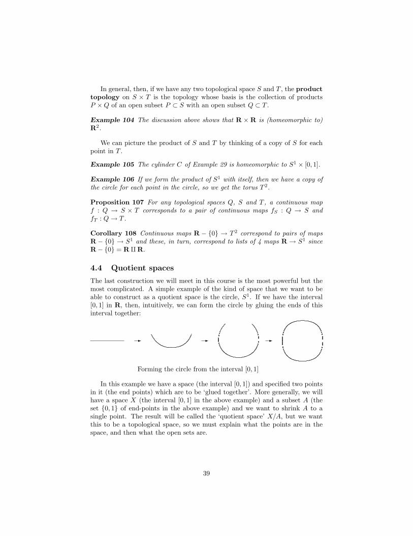
In general, then, if we have any two topological space S and T , the producttopology on S × T is the topology whose basis is the collection of productsP ×Q of an open subset P ⊂ S with an open subset Q ⊂ T .

Example 104 The discussion above shows that R ×R is (homeomorphic to)R2.

We can picture the product of S and T by thinking of a copy of S for eachpoint in T .

Example 105 The cylinder C of Example 29 is homeomorphic to S1 × [0, 1].

Example 106 If we form the product of S1 with itself, then we have a copy ofthe circle for each point in the circle, so we get the torus T 2.

Proposition 107 For any topological spaces Q, S and T , a continuous mapf : Q → S × T corresponds to a pair of continuous maps fS : Q → S andfT : Q→ T .

Corollary 108 Continuous maps R − {0} → T 2 correspond to pairs of mapsR − {0} → S1 and these, in turn, correspond to lists of 4 maps R → S1 sinceR− {0} = RqR.

4.4 Quotient spaces

The last construction we will meet in this course is the most powerful but themost complicated. A simple example of the kind of space that we want to beable to construct as a quotient space is the circle, S1. If we have the interval[0, 1] in R, then, intuitively, we can form the circle by gluing the ends of thisinterval together:

- - -

Forming the circle from the interval [0, 1]

In this example we have a space (the interval [0, 1]) and specified two pointsin it (the end points) which are to be ‘glued together’. More generally, we willhave a space X (the interval [0, 1] in the above example) and a subset A (theset {0, 1} of end-points in the above example) and we want to shrink A to asingle point. The result will be called the ‘quotient space’ X/A, but we wantthis to be a topological space, so we must explain what the points are in thespace, and then what the open sets are.

39

The quotient space X/A is the set X−A∪{∗} consisting of the complementof A in X together with one extra point, labelled ∗. To define the topology onX/A, note that there is a function π : X → X/A defined by

π(x) ={

x if x ∈ X −A* if x ∈ A

called the canonical projection. We then say that a subset U ⊂ X/A is openif (and only if) the preimage π−1(U) is an open subset of X. It is straightforwardto verify that this satisfies the axioms and so forms a topology on X/A.

Example 109 Let X = [0, 1] and A = {0, 1} as above. As a set X/A =(0, 1) ∪ {∗}, and a subset U ⊂ X/A is open if π−1(U) is open in [0, 1], where

π(x) ={

t if t ∈ (0, 1)* if t = 0of t = 1

For example, let U ⊂ X/A be the subset (0, 12 ) ∪ {∗}. Then π−1(U) = (0, 1

2 ) ∪{0, 1} = [0, 1

2 ) ∪ {1}. This is not an open subset of [0, 1] as the space 1 has nobreathing space about it. Therefore U is not an open set in the quotient spaceX/A.

Example 110 Let X = [0, 1] × [0, 1] be a solid square, and let A = ∂X =[0, 1]× {0, 1} ∪ {0, 1} × [0, 1] be the boundary of the square. Then X/A ∼= S2.

Similarly, if X is a solid disc D2 and A = ∂X = S1 is the boundary, thenX/A is homeomorphic to S2.

Forming a quotient space X/A is one type of gluing construction, as we have‘glued’ all the points of A together to a single point. But there are more generalquotient spaces where we glue points together, but not all to the same point.

For example, we could take X = [0, 1]× [0, 1] to be the solid square, and wemight want to glue opposite edges of the square together to get a cylinder. Sincewe are not gluing all these edge points to one single point, this construction doesnot fit the above definition of quotient space. So we extend the definition asfollows. What we need to allow is to have an equivalence relation ∼ defined onX, with x ∼ y indicating that the two points x and y are to be glued together.

Example 111 Let X = [0, 1] × [0, 1] and define an equivalence relation ∼ onX by

x ∼ y if{

either x = x′ and y = y′

or x = x′ and |y − y′| = 1

so that two different points (x, y) and (x′, y′) are equivalent only if x = x′ and yand y′ differ by 1, i.e. one point is on one edge, and the other point is directlyabove or below it on the other edge.

Given an equivalence relation ∼ on a set X we can form the set X/∼ ofequivalence classes. There is always a projection function π : X → X/∼ given

40

by sending a point of X to the equivalence class containing that point. If X isa topological space and ∼ is an equivalence relation on X, then the quotientspace X/∼ is the set of equivalence relations with the topology defined byU ⊂ X/∼ is open if, and only if, π−1(U) is open in X.

If we want to form X/A, then we can express it in this language by definingan equivalence relation by

x ∼ y if{

either x = x′

or x ∈ A and y ∈ A

Then X/∼= X/A, so the collapsing-a-subset type of quotient space (X/A) isjust a special case of the equivalence-relation quotient space (X/∼).

Theorem 112 Suppose that Q is a quotient of a topological space T under theequivalence relation ∼. If S is any other topological space and f : Q → S is acontinuous function, then we can compose f with the projection π : T → Q toget a function T → S which will also be continuous. In other words, given afunction f as in the diagram, there is a function T → S, as shown by a dottedline, such that the diagram commutes.

T

?π

QR

S-

Conversely, if f : T → S is any continuous function such that f(x) = f(y)whenever x ∼ y, then there is a corresponding continuous function f : Q → Ssuch that f ◦ π = f , i.e. the following diagram commutes

T

?π

Q

@@

@@RS-

These give a one-to-one correspondence between

{ continuous maps Q→ S }

and

{ continuous maps T → S such that f(x) = f(y) whenever x ∼ y }

Proof If π : T → Q is the projection then we can turn a map f : Q→ S into amap T → S by composition:

f ◦ π : T → S.

This will be continuous as both f and π are.

41

Conversely, if f : T → S is continuous and f(x) = f(y) whenever x ∼ y,then we can derive a map f : Q → S by f(E) = f(x) if E is an equivalenceclass and x a member of E. The key point is that if y is another member of Ethen x ∼ y, so f(x) = f(y) and g(E) = f(y). Thus it does not matter whichmember of E we choose, as f gives the same value on each of them. And wecertainly have f ◦ π = f .

To show that this map f is continuous, let R be an open subset of S. Then

f−1(R) = (f ◦ π)−1(R) = π−1(f−1(R)).

The function f is continuous, so f−1(R) is open, i.e. π−1(f−1(R)) is open.And the topology on Q was defined so that the preimage π−1 of a set is openprecisely when the set is open. So π−1(f−1(R)) being open means that f−1(R)is open. Hence f is continuous. •

This result is very helpful when studying any map whose domain is a quotientspace. And with the following result we will be able to easily identify many ofthe quotient spaces we are interested in.

Lemma 113 If X is a compact topological space and ∼ is any equivalence re-lation on X, then X/∼ is compact.

Proof π : X → X/∼ is continuous and surjective so, by Proposition 65, X/∼is compact. •

Proposition 114 [0, 1]/{0, 1} is homeomorphic with S1.

Proof The exponential map restricts to a continuous map e : [0, 1]→ S1 whichis surjective. By the Theorem, this corresponds to a map [0, 1]/{0, 1} → S1

which is also surjective. Moreover, since e(x) = e(y) only when x − y is aninteger, we see that e corresponds to an injective map [0, 1]/{0, 1} → S1. Bythe Lemma, [0, 1]/{0, 1} is compact, and S1 is Hausdorff, so this continuousbijection [0, 1]/{0, 1} → S1 is a homeomorphism. •

Using this result and the Theorem gives a way of understanding continuousmaps from S1 which we will exploit in the next section.

Example 115 For any topological space T , a function f : S1 → T can beconsidered as a function f : [0, 1] → T . And any map g : [0, 1] → T with theproperty that g(0) = g(1) can be considered as a map S1 → T . This way ofdealing with maps from S1 is very helpful as we will see later, as it is quite easyto understand maps from [0, 1], and not hard to keep track of g(0) and g(1).

Similarly, we can quotient the square by identifying two opposite edges andthis will give the cylinder.

Example 116 If X = [0, 1]× [0, 1] with the relation

x ∼ y if{

either x = x′ and y = y′

or x = x′ and |y − y′| = 1,

42

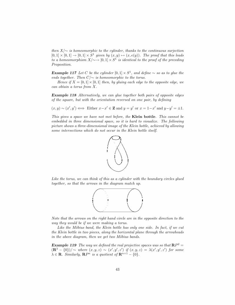
then X/∼ is homeomorphic to the cylinder, thanks to the continuous surjection[0, 1]× [0, 1] → [0, 1]× S1 given by (x, y) 7→ (x, e(y)). The proof that this leadsto a homeomorphism X/∼→ [0, 1]×S1 is identical to the proof of the precedingProposition.

Example 117 Let C be the cylinder [0, 1]× S1, and define ∼ so as to glue theends together. Then C/∼ is homeomorphic to the torus.

Hence if X = [0, 1]× [0, 1] then, by gluing each edge to the opposite edge, wecan obtain a torus from X.

Example 118 Alternatively, we can glue together both pairs of opposite edgesof the square, but with the orientation reversed on one pair, by defining

(x, y) ∼ (x′, y′)⇐⇒ Either x−x′ ∈ Z and y = y′ or x = 1−x′ and y−y′ = ±1.

This gives a space we have not met before, the Klein bottle. This cannot beembedded in three dimensional space, so it is hard to visualize. The followingpicture shows a three-dimensional image of the Klein bottle, achieved by allowingsome intersections which do not occur in the Klein bottle itself.

Like the torus, we can think of this as a cylinder with the boundary circles gluedtogether, so that the arrows in the diagram match up.

6? ?

6

Note that the arrows on the right hand circle are in the opposite direction to theway they would be if we were making a torus.

Like the Mobius band, the Klein bottle has only one side. In fact, if we cutthe Klein bottle in two pieces, along the horizontal plane through the arrowheadsin the above diagram, then we get two Mobius bands.

Example 119 The way we defined the real projective spaces was so that RP 2 =(R3 − {0})/∼ where (x, y, z) ∼ (x′, y′, z′) if (x, y, z) = λ(x′, y′, z′) for someλ ∈ R. Similarly, RPn is a quotient of Rn+1 − {0}.

43

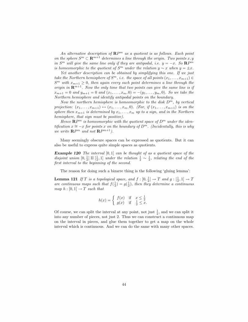
An alternative description of RPm as a quotient is as follows. Each pointon the sphere Sm ⊂ Rm+1 determines a line through the origin. Two points x, yin Sm will give the same line only if they are antipodal, i.e. y = −x. So RPm

is homeomorphic to the quotient of Sm under the relation y ∼ x when y = ±x.Yet another description can be obtained by simplifying this one. If we just

take the Northern hemisphere of Sm, i.e. the space of all points (x1, . . . , xm+1) ∈Sm with xm+1 ≥ 0, then again every such point determines a line through theorigin in Rm+1. Now the only time that two points can give the same line is ifxm+1 = 0 and ym+1 = 0 and (x1, . . . , xm, 0) = −(y1, . . . , ym, 0). So we take theNorthern hemisphere and identify antipodal points on the boundary.

Now the northern hemisphere is homeomorphic to the disk Dm, by verticalprojection: (x1, . . . , xm+1) ↔ (x1, . . . , xm, 0). (For, if (x1, . . . , xm+1) is on thesphere then xm+1 is determined by x1, . . . , xm up to a sign, and in the Northernhemisphere, that sign must be positive).

Hence RPm is homeomorphic with the quotient space of Dm under the iden-tification x ∼= −x for points x on the boundary of Dm. (Incidentally, this is whywe write RPm and not RPm+1).

Many seemingly obscure spaces can be expressed as quotients. But it canalso be useful to express quite simple spaces as quotients.

Example 120 The interval [0, 1] can be thought of as a quotient space of thedisjoint union [0, 1

2 ] q [ 12 , 1] under the relation 12 ∼

12 , relating the end of the

first interval to the beginning of the second.

The reason for doing such a bizarre thing is the following ‘gluing lemma’:

Lemma 121 If T is a topological space, and f : [0, 12 ] → T and g : [12 , 1] → T

are continuous maps such that f( 12 ) = g( 1

2 ), then they determine a continuousmap h : [0, 1]→ T such that

h(x) ={

f(x) if x ≤ 12

g(x) if 12 ≤ x.

Of course, we can split the interval at any point, not just 12 , and we can split it

into any number of pieces, not just 2. Thus we can construct a continuous mapon the interval in pieces, and glue them together to get a map on the wholeinterval which is continuous. And we can do the same with many other spaces.

44

5 Homotopy

One ultimate goal of topology is to list all the continuous functions with a givendomain and range. Of course that is nearly always impossible because thereare far, far too many. If, however, we allow some leeway, and consider somefunctions as equal to others, then the problem becomes more feasible. Onecriteria for considering two functions to be equal is the notion of ‘homotopy’.

For example, let f : [0, 2] → R be the function f(x) = 1 + x2(x − 2)2,depicted below.

- x

6

f(x)

0 2

1

This is almost a constant function to 1, but with a small deviation around x = 1.If we take the function f1(x) = 1 + 1

2x2(x− 2)2, then this has a similar shape,but with a smaller deviation. Similarly, f2(x) = 1 + 1

3x2(x − 2)2 has the sameshape but with an even smaller deviation.

- x

6f(x)

f2(x)

f1(x)R

0 1

1

Carrying on, for each n ≥ 1, we can define fn(x) = 1+ 1(n+1)x

2(x−2)2, and thusobtain a family of functions interpolating between f and the constant function.

However, this interpolationg process allows us to jump from f1 to f2, andfrom f2 to f3 and so on. It is not a continuous process so, instead, we shouldparametrize the interpolating functions by real numbers in some range, not byintegers. So we require that there be functions ft, one for each t ∈ [0, 1]. In thatcase we would consider f0 and f1 to be equivalent. However, we need some sortof continuity in t: if t is close to t′, then ft ought to be close to ft′ . The easiestway to do that is as follows.

Definition: If f, g : S → T are continuous maps and there is anothercontinuous map F : S × [0, 1]→ T such that

F (x, 0) = f(x) and F (x, 1) = g(x)

for all x ∈ S, then f and g are said to be homotopic, written f ' g, andF is a homotopy between f and g.

Example 122 Let f : S1 → R2 be the natural inclusion map, and let g : S1 →R2 be the constant map g(x) = (0, 0) for all x ∈ S1. These two maps arehomotopic, for let

F : S1 × [0, 1]→ R2

be defined byF ((x, y), t) = ((1− t)x, (1− t)y).

45

Then F is continuous, because it is a composite of additions and multiplications.And F ((x, y), 0) = (1x, 1y) = (x, y) = f(x, y). And F ((x, y), 1) = (0x, 0y) =(0, 0) = g(x, y).

Example 123 Let f : [0, 2]→ [0, 2] be the identity map and let g : [0, 2]→ [0, 2]be the constant map g(x) = 0 for all x. Then there is a homotopy between thesemaps given by

F : [0, 2]× [0, 1]→ [0, 2]

F (x, t) = (1− t)x.

Example 124 Let f, g : R→ R be any two continuous functions. Define

F : R× [0, 1]→ R

by F (x, t) = (1 − t)f(x) + tg(x). Then F is continuous, being a composite ofcontinuous functions, F (x, 0) = (1 − 0)f(x) + 0 = f(x) and F (x, 1) = 0 +1g(x) = g(x), so F is a homotopy between f and g. In other words, any pair ofcontinuous functions on R are homotopic.

Lemma 125 Let f : S → T be any continuous map. Then f ' f .

Proof We can define a homotopy

F : S × [0, 1]→ T

by F (x, t) = f(x) for all t. Then F (x, 0) = f(x) and F (x, 1) = f(x). •

Lemma 126 Let f, g : S → T be two continuous maps. If F is a homotopybetween f and g, then there is also a homotopy between g and f .

Proof If F (x, 0) = f(x) and F (x, 1) = g(x), then define

G : S × [0, 1]→ T

by G(x, t) = F (x, 1− t). Then G(x, 0) = g(x) and G(x, 1) = f(x). •

Lemma 127 Let f, g, h : S → T be three continuous maps. If f and g arehomotopic and g and h are homotopic, then f and h are homotopic.

Proof Let F : S × [0, 1] → T be a continuous map such that F (x, 0) = f(x)and F (x, 1) = g(x), and let G : S × [0, 1] → T be a continuous map suchthat G(x, 0) = g(x) and G(x, 1) = h(x). Define a further continuous mapH : S × [0, 1]→ T by

H(x, t) ={

F (x, 2t) if 0 ≤ t ≤ 12

G(x, 2t− 1) if 12 ≤ t ≤ 1

•

So homotopy is an equivalence relation between continuous functions whichmeans we can consider ‘homotopy classes’ of continuous maps. We write [S, T ]for the set of homotopy classes of maps S → T , i.e. equivalence classes ofcontinuous maps under the equivalence relation of homotopy.

46

5.1 Homotopy equivalence

Having defined homotopy (a relation between functions), we can now define ho-motopy equivalence (which is a relation between spaces), by taking the definitionof homeomorphism and inserting some homotopies.

Definition: Let S and T are two topological spaces. If f : S → T andg : T → S are continuous maps such that

(g ◦ f) ' 1S and (f ◦ g) ' 1T ,

where 1S is the identity map on S and 1T is the identity map on T , thenwe say that S and T are homotopy equivalent, and that f and g arehomotopy equivalences.

Example 128 If S is a space containing a single point, then S and R arehomotopy equivalent. To see this, define f : R→ S to be the constant function(there is no choice as to how to define f), and let g : S → R be the functionwhich takes the single point in S to 0 in R. The composite f ◦ g : S → S isthe identity map, while the composite g ◦ f : R → R is the constant functionto 0. Since all functions R → R are homotopic, by Example 124, so g ◦ f ishomotopic to the identity.

Example 129 Let A be the annulus

A = {(x, y) ∈ R2 : 1 ≤√

x2 + y2 ≤ 2}.

Then A ' S1 as follows. Define f : S1 → A to be the natural inclusionf(x, y) = (x, y), and g : A → S1 to be the radial projection inwards whichcan be described algebraically as

g(x, y) =1√

x2 + y2(x, y).

Now, g ◦ f is the identity on S1 because, if (x, y) ∈ S1, then g(x, y) = (x, y).This is certainly homotopic to the identity, by Lemma 125.

And (f ◦ g)(x, y) = 1√x2+y2

(x, y). This is homotopic to the identity on A by

the homotopy F : A× [0, 1]→ A defined by

F ((x, y), t) =t√

x2 + y2 + (1− t)√x2 + y2

(x, y).

(Check: this is continuous, being a composite of continuous maps; F ((x, y), 0) =(f ◦ g)(x, y) and F ((x, y), 1) = (x, y).)

Hence f and g form a homotopy equivalence between A and S1.

Lemma 130 If S and T are homeomorphic, then they are also homotopy equiv-alent.

47

Proof If we have homeomorphisms f : S → T and g : T → S, then f ◦ g andg ◦ f are the respective identity maps, so these composites are homotopic to therespective identity maps by Lemma 125. •

Of course, there are many pairs of spaces which are homotopy equivalentbut not homeomorphic.

Example 131 The open interval (0, 1) is homotopy equivalent to {0}. We candefine f : (0, 1) → 0, and define g : {0} → (0, 1) by g(0) = 1

2 . With thischoice of g, a homotopy from (g ◦ f) to the identity map of (0, 1) is given byH : (0, 1)× [0, 1]→ (0, 1) defined by

H(x, t) =1− t

2+ tx.

The image H(x, t) is certainly contained in (0, 1) if x, t ∈ (0, 1) × [0, 1], andH is continuous, being a composite of multiplications and additions. The sameargument shows that [0, 1] is homotopy equivalent to {0} as well.

A space like (0, 1) or [0, 1], which is homotopy equivalent to a one-pointspace (such as {0}), is said to be contractible. Example 128 above shows thatR is contractible.

Proposition 132 If S is contractible and T is any topological space then anytwo continuous functions f, g : T → S are homotopic. In particular, any con-tinuous function to a contractible space is homotopic to a constant map.

Proof Let f, g : T → S be two continuous maps. If S is contractible, then thereare continuous maps h : S → {0} and j : {0} → S such that h ◦ j ' 1 andj ◦ h ' 1. In particular,

f = (1 ◦ f) ' (j ◦ h ◦ f) and g = (1 ◦ g) ' (j ◦ h ◦ g).

Since h ◦ f : T → {0}, so j ◦ h ◦ f : T → S must be the constant map t 7→ j(0)for all t ∈ T . Similarly j ◦ h ◦ g is this same constant map, and so f ' g. •

Contractible spaces are thus uninteresting from a homotopy point of view:all functions to them are homotopic, and homotopic to constant maps. Since Ris contractible, this confirms that all functions from R to R are homotopic, aswe saw in Example 128. But are there any ‘interesting’ spaces?

Proposition 133 The 2-point space S0 is not contractible.

Proof Suppose that S0 is contractible, with homotopy equivalences f : S0 →{0} and g : {0} → S0. Then f ◦ g : {0} → {0} has to be the identity, and(g ◦ f) : S0 → S0 is homotopic to the identity. So there is a homotopy

F : S0 × I → S0

with F (x, 0) = x and F (x, 1) = g(f(x)) = g(0).

48

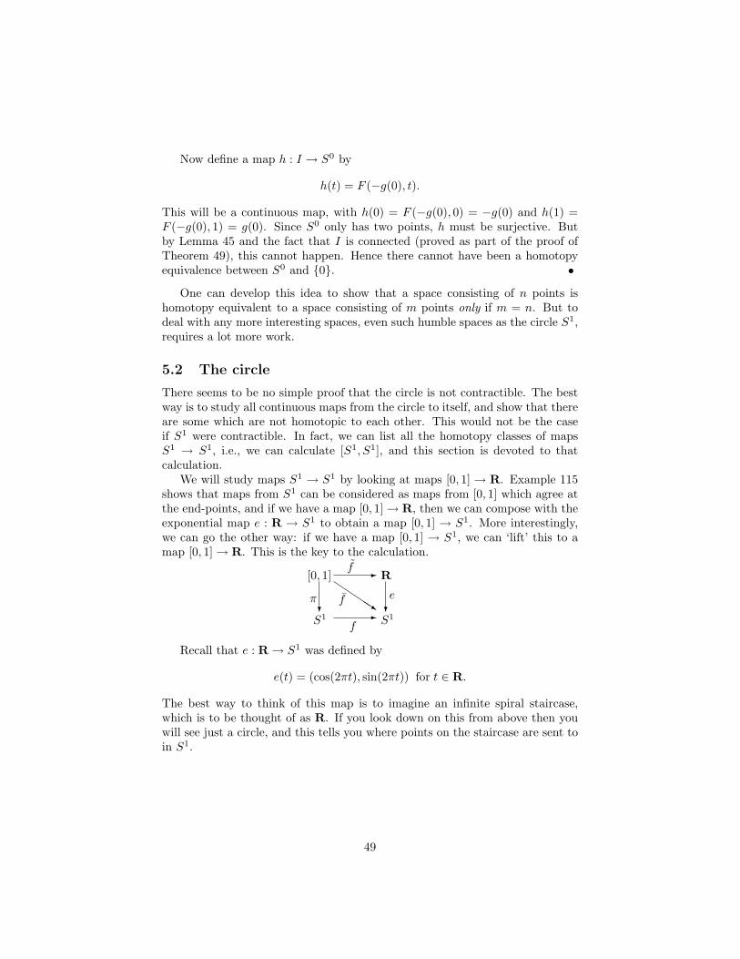
Now define a map h : I → S0 by

h(t) = F (−g(0), t).

This will be a continuous map, with h(0) = F (−g(0), 0) = −g(0) and h(1) =F (−g(0), 1) = g(0). Since S0 only has two points, h must be surjective. Butby Lemma 45 and the fact that I is connected (proved as part of the proof ofTheorem 49), this cannot happen. Hence there cannot have been a homotopyequivalence between S0 and {0}. •

One can develop this idea to show that a space consisting of n points ishomotopy equivalent to a space consisting of m points only if m = n. But todeal with any more interesting spaces, even such humble spaces as the circle S1,requires a lot more work.

5.2 The circle

There seems to be no simple proof that the circle is not contractible. The bestway is to study all continuous maps from the circle to itself, and show that thereare some which are not homotopic to each other. This would not be the caseif S1 were contractible. In fact, we can list all the homotopy classes of mapsS1 → S1, i.e., we can calculate [S1, S1], and this section is devoted to thatcalculation.

We will study maps S1 → S1 by looking at maps [0, 1] → R. Example 115shows that maps from S1 can be considered as maps from [0, 1] which agree atthe end-points, and if we have a map [0, 1]→ R, then we can compose with theexponential map e : R → S1 to obtain a map [0, 1] → S1. More interestingly,we can go the other way: if we have a map [0, 1] → S1, we can ‘lift’ this to amap [0, 1]→ R. This is the key to the calculation.

[0, 1]

?π

S1 - S1f

QQ

QQs

- R

?ef

f

Recall that e : R→ S1 was defined by

e(t) = (cos(2πt), sin(2πt)) for t ∈ R.

The best way to think of this map is to imagine an infinite spiral staircase,which is to be thought of as R. If you look down on this from above then youwill see just a circle, and this tells you where points on the staircase are sent toin S1.

49

? ? ?

1

−1

0

1

2

The map e : R→ S1

The highlighted part of the spiral shows the preimage under e of the highlightedpart of the circle.

The first result we need is the ‘lifting’ theorem that maps [0, 1]→ S1 can be‘lifted’ to maps [0, 1]→ R.

Proposition 134 (Path-lifting) If f : [0, 1] → S1 is a continuous function,then for any point x ∈ R such that e(x) = f(0), there is a unique continuousfunction f : [0, 1]→ R such that ef(t) = f(t) for all t ∈ [0, 1] and f(0) = x.

The way to think of this statement is to think of the parameter t ∈ [0, 1] asspecifying a moment in time. As t runs from 0 to 1, so f traces out a path inS1. The condition ef(t) = f(t) specifies that f(t) must always be above f(t) inthe spiral staircase picture. It is as if one person is walking around a circle, andsomeone else is on a spiral staircase and determined to always be directly abovethe first person. Clearly they can always do that if they move fast enough, butthere is no choice about where they move.Proof We will construct f bit by bit. The key to this is that if we take any‘proper’ subset U of S1 (i.e., any subset except the whole of S1), then its preim-age under e is a disjoint union of infinitely many spaces, each homeomorphic toU . Now suppose we have a small interval [δ1, δ2] ⊂ [0, 1] whose image, underf , is contained in U . And suppose that f(δ1) is already defined in such a waythat ef(δ1) = f(δ1). Then f(δ1) lies in one of these spaces homeomorphic to U .We can then compose that homeomorphism with f to define f on the interval[δ1, δ2] so as to agree with the value on δ1.

So, then, we need a few subsets of S1 (two, in fact, are sufficient) such thatwe can partition the interval [0, 1] by smaller closed intervals such that the imageof each, under f , is entirely contained in one of our subsets of S1.

Let U = S1 − {1} be the open subset of circle containing every point apartfrom 1, and let V = S1−{−1} be the open subset containing every point apartfrom −1.

50

The preimages f−1(U) and f−1(V ) will be open subsets of [0, 1]. Hence, foreach point x in f−1(U), there will be some δ such that the interval (x− δ, x +δ)∩ [0, 1] is contained in f−1(U). This set (x− δ, x+ δ)∩ [0, 1] is an open subsetof [0, 1]. Thus, by considering every point x of f−1(U), we get an open coveringof f−1(U) by intervals.

Doing the same for f−1(V ) we can get an open covering of f−1(U). SinceU ∪ V = S1, so f−1(U) ∪ f−1(V ) = [0, 1]. Thus, if we put these two opencoverings (of f−1(U) and f−1(V )) together, we get an open covering of [0, 1].Now [0, 1] is compact, so we can refine this open covering to get a finite coveringI1, I2, . . . , In, with the property that, for each i, either Ii ⊂ f−1(U) or Ii ⊂f−1(V ).

If these cover [0, 1] then, as we travel from 0 to 1, we will always be inside(at least) one of these sets Ii. Let’s agree to order them according to which oneswe meet as we go from 0 to 1. So 0 ∈ I1, 1 ∈ In. Since all the Ii’s are opensubsets of [0, 1], we can find numbers δ0, . . . , δn such that δ0 = 0, δn = 1 andδi ∈ Ii ∩ Ii+1 for 0 < i < n.

δ0

0[

I1 b1)

a2(

I2 b2)

δ1

a3(

I3 b3)

δ2

a4(

δ3

Thus [δi, δi+1] ⊂ Ii+1 for each i < n and the union of all these closed intervalswill be [0, 1]. We will construct f by defining it on each of these closed intervalsin turn.

We must have f(0) = x, and we can think of this as determining f on theinterval [0, δ0]. This will serve as the first step of an induction argument.

To continue, suppose that we have f defined and continuous on the interval[0, δi]; we wish to extend this definition to the larger interval [0, δi+1]. We do thisby defining a continuous function f on [δi, δi+1] such that f(δi) = f(δi). Withsuch a function f , the definition and continuity of f on [0, δi+1] follow from avariant of Lemma 121 (where 1

2 and 1 are replaced by δi and δi+1 respectively).By construction [δi, δi+1] is either contained in f−1(U) or in f−1(V ) (or

possibly both). Suppose, for now, that it is contained in f−1(U). So we canthink of f as restricting to a map [δi, δi+1]→ U . If ef(δi) = f(δi) then ef(δi) ∈U , so f(δi) cannot be an integer (for e(n) = 1 6∈ U for all n ∈ Z). Hence thereis some open interval (n, n+1), where n is an integer, which contains f(δi). Wecan define a map gn

U : U → (n, n + 1) by

gnU : (cos(2πφ), sin(2πφ)) 7→ n + φ,

where we take φ to be in the range 0 < φ < 1. This is continuous, and has theproperty that e ◦ gn

U is the identity on U . So gnU (f(δi)) = f(δi). We then define

f to be the composite

[δi, δi+1]f−→ U

gnU−→ (n, n + 1) ↪→ R.

51

This will be continuous, as it is a composite of continuous maps, and f(δi) =gn

U (f(δi)) = f(δi). This completes the proof of the inductive step for the casewhere [δi, δi+1] ⊂ f−1(U).

If [δi, δi+1] ⊂ f−1(V ) then we can restrict f to a map [δi, δi+1] → V . Thenf(δi) must lie in some interval (n− 1

2 , n + 12 ) for some integer n. We can define

a map gnV : V → (n− 1

2 , n + 12 ) by

gnV : (cos(2πφ), sin(2πφ)) 7→ n + φ,

where we now take φ to be in the range − 12 < φ < 1

2 . Then we define f to bethe composite

[δi, δi+1]f−→ V

gnV−→ (n− 1

2, n +

12) ↪→ R.

As before, this is continuous, being a composite of continuous maps, and f(δi) =gn

V (f(δi)) = f(δi). Thus, in either case, the inductive step is complete and wecan deduce the existence of a continuous map f : [0, 1]→ R such that f(0) = x.

Finally, suppose that f : [0, 1]→ R is another lift of f with f(0) = x = f(0).Since e◦ f = e◦f we see that f(y)− f(y) ∈ Z for all y. Thus we get a continuousmap f − f : [0, 1] → Z. By Lemma 55, this map must be constant. Sincef(0) = f(0) = x, we conclude that f(y)− f(y) = 0 for all y, i.e. f = f . Hencethe lift f is unique. •

This enables us to define the degree of a continuous map f : S1 → S1. Pickany point x ∈ R such that e(x) = f(0). Lift f to a path f such that f(0) = x.Then the degree of f is defined to be the integer f(1)− f(0).

This is dependent only on f . For suppose we picked another point y ∈R with e(y) = f(0), and a lift f such that f(0) = y. Then the functionf : [0, 1] → R defined by f(t) = x − y + f(t) would satisfy f(0) = x ande(f)(t) = e(x)−e(y)+ef(t) = f(t). Thus f would be another lift of f beginningat x. By uniquenss, f = f . Hence f(1)− f(0) = f(1)− f(0) = f(1)− f(0). Sothe degree of f as calculated using f would be the same as the degree of f ascalculated using f .

Example 135 Any constant function S1 → S1 has degree 0, for the lift f canbe taken to be constant: f(t) = x for all t, where x is chosen so that e(x) = f(0).Hence deg(f) = 0

Example 136 The identity map S1 → S1 has degree 1. For a lift f is givenby f(t) = t.

Example 137 If f is the map

f(cos(θ), sin(θ)) = (cos(2θ), sin(2θ))

then a lift f is given by f(t) = 2t, so deg(f) = 2.

52

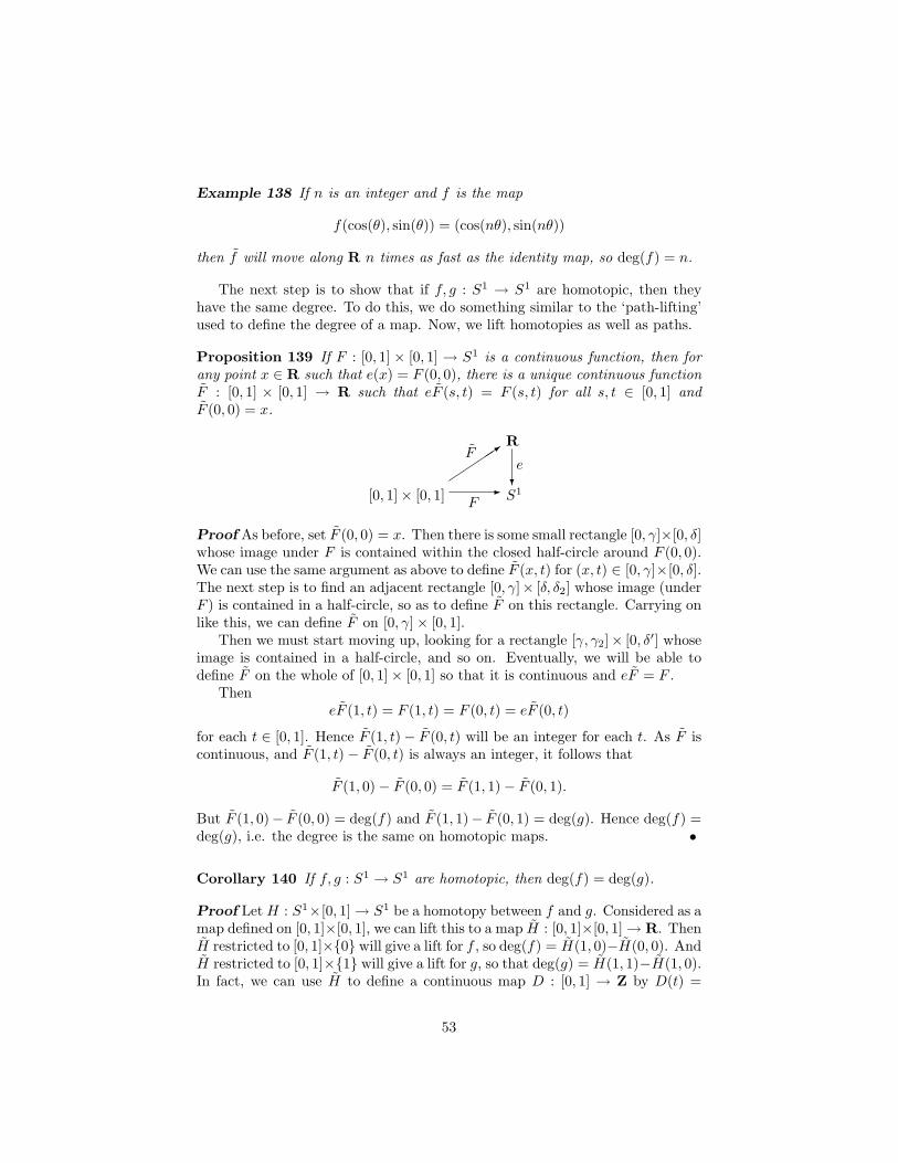
Example 138 If n is an integer and f is the map

f(cos(θ), sin(θ)) = (cos(nθ), sin(nθ))

then f will move along R n times as fast as the identity map, so deg(f) = n.

The next step is to show that if f, g : S1 → S1 are homotopic, then theyhave the same degree. To do this, we do something similar to the ‘path-lifting’used to define the degree of a map. Now, we lift homotopies as well as paths.

Proposition 139 If F : [0, 1] × [0, 1] → S1 is a continuous function, then forany point x ∈ R such that e(x) = F (0, 0), there is a unique continuous functionF : [0, 1] × [0, 1] → R such that eF (s, t) = F (s, t) for all s, t ∈ [0, 1] andF (0, 0) = x.

[0, 1]× [0, 1] - S1F

��

��3R

?e

F

Proof As before, set F (0, 0) = x. Then there is some small rectangle [0, γ]×[0, δ]whose image under F is contained within the closed half-circle around F (0, 0).We can use the same argument as above to define F (x, t) for (x, t) ∈ [0, γ]×[0, δ].The next step is to find an adjacent rectangle [0, γ]× [δ, δ2] whose image (underF ) is contained in a half-circle, so as to define F on this rectangle. Carrying onlike this, we can define F on [0, γ]× [0, 1].

Then we must start moving up, looking for a rectangle [γ, γ2]× [0, δ′] whoseimage is contained in a half-circle, and so on. Eventually, we will be able todefine F on the whole of [0, 1]× [0, 1] so that it is continuous and eF = F .

TheneF (1, t) = F (1, t) = F (0, t) = eF (0, t)

for each t ∈ [0, 1]. Hence F (1, t)− F (0, t) will be an integer for each t. As F iscontinuous, and F (1, t)− F (0, t) is always an integer, it follows that

F (1, 0)− F (0, 0) = F (1, 1)− F (0, 1).

But F (1, 0)− F (0, 0) = deg(f) and F (1, 1)− F (0, 1) = deg(g). Hence deg(f) =deg(g), i.e. the degree is the same on homotopic maps. •

Corollary 140 If f, g : S1 → S1 are homotopic, then deg(f) = deg(g).

Proof Let H : S1×[0, 1]→ S1 be a homotopy between f and g. Considered as amap defined on [0, 1]×[0, 1], we can lift this to a map H : [0, 1]×[0, 1]→ R. ThenH restricted to [0, 1]×{0} will give a lift for f , so deg(f) = H(1, 0)−H(0, 0). AndH restricted to [0, 1]×{1} will give a lift for g, so that deg(g) = H(1, 1)−H(1, 0).In fact, we can use H to define a continuous map D : [0, 1] → Z by D(t) =

53

H(1, t) − H(0, t). Then deg(f) = D(0) and deg(g) = D(1). However, byLemma 55, such a function D must be constant, since [0, 1] is connected. Hencedeg(f) = deg(g). •

Corollary 141 The circle is not contractible.

Proof Suppose that f : S1 → {0} and g : {0} → S1 are homotopy equivalences.So g ◦ f ' 1S1 . Now, (g ◦ f)(x) = g(0) for all x, i.e. g ◦ f is a constant function,and hence has degree 0. Conversely, the identity map has degree 1. As theseare different, g ◦ f cannot be homotopic to 1S1 , so S1 is not contractible. •

The final step in our computation of [S1, S1] is to see that two maps havethe same degree only when they are homotopic; this is the converse to Corollary140.

Theorem 142 If f, g : S1 → S1 are such that deg(f) = deg(g), then f and gare homotopic.

Proof The idea is to define a homotopy ‘upstairs’. Lift f and g to mapsf , g : [0, 1]→ R so that ef = f ◦π and eg = g ◦π. Define H : [0, 1]× [0, 1]→ S1

byH(s, t) = e(tf(s) + (1− t)g(s)).

This is constant being a composite of continuous functions, and

H(s, 0) = eg(s) = g(π(s)) and H(s, 1) = ef(s) = f(π(s)).

Now, if d = deg(f) = deg(g), then f(1) = d + f(0) and g(1) = d + g(0), so

H(1, t) = e(tf(1) + (1− t)g(1)) = e(t(d + f(0)) + (1− t)(d + g(0)))= e(td + tf(0) + (1− t)d + (1− t)g(0)) = e(d + (tf(0) + (1− t)g(0)))= e(tf(0) + (1− t)g(0)) since d ∈ Z= H(0, t).

Thus H corresponds to a map F : S1× [0, 1]→ S1 with F (π(s), t) = H(s, t), soF (s, 0) = g(s) and F (s, 1) = f(s). Hence F is a homotopy from g to f . •

Corollary 143 [S1, S1] = Z.

Proof Every continuous map S1 → S1 has a degree, which is an integer. Ho-motopic maps have the same degree, so this gives a function [S1, S1]→ Z. Thisis surjective by Example 138. And it is injective by the preceding Theorem. •

5.3 Brouwer’s fixed point theorem

We have already seen a theorem saying that any continuous map from [0, 1] toitself must have a fixed point. Our study of continuous maps from S1 to S1 canbe used to prove a two-dimensional version of this theorem, due to Brouwer.

54

Theorem 144 Let f : D2 → D2 be a continuous map, where D2 is the closeddisk

D2 = {(x, y) ∈ R2 : x2 + y2 ≤ 1}.Then f has a fixed point, i.e. there is some (x, y) ∈ D2 for which f(x, y) =(x, y).

Proof Suppose that f : D2 → D2 does not have a fixed point, so that f(x, y) 6=(x, y) for all (x, y) ∈ D2. So, for each point (x, y) ∈ D2 we get two points (x, y)and f(x, y), and we can draw a line through them both. Extend this line beyond(x, y) until it meets the boundary of D2 (i.e. S1), and let g(x, y) be the pointwhere this happens. So we get a function g : D2 → S1 as in the picture.

f(x,y)•�

����•

(x,y) •g(x,y)

This map g is continuous, by construction and, if (x, y) is on the boundaryof D2, then g(x, y) = (x, y) no matter what f(x, y) is.

Now define a mapF : S1 × [0, 1]→ S1

by F ((x, y), t) = g(tx, ty).This map F is continuous, so we can think of it as a homotopy between the

map h : S1 → S1 defined by h(x, y) = F ((x, y), 0) and j : S1 → S1 defined byj(x, y) = F ((x, y), 1). Now h(x, y) = g(0) for all (x, y), so h is a constant mapand thus deg(h) = 0. On the other hand, however, j(x, y) = g(x, y) = (x, y) forall (x, y), so j is the identity map and deg(j) = 1. If F really is a homotopybetween h and j then these degrees must be equal. Since they are not, the mapF cannot exist. Hence nor can g, showing in turn that the map f must havehad a fixed point in the first place. •

5.4 Vector Fields

Probably the most famous theorem of topology is the ‘Hairy ball theorem’. Insimple language this says that you cannot comb a hairy ball. To make this moreprecise, we need the notion of a ‘vector field’.

When we comb a surface then, at each point in that surface, we move thecomb in a certain direction, tangential to the surface. So we have a functionwhich assigns, to each point on the surface, a direction, i.e. a vector, which istangential to the surface. Of course, we want this function to be continuous. Acontinuous vector-valued function is called a vector field, and if the vector isalways tangential to the surface then it is called a tangential vector field.

Example 145 A simple example of a tangential vector field assigns, to eachpoint on the surface of the earth, a vector representing the wind felt at thatpoint.

55

Example 146 Another example of a tangential vector field is given by combinga hairy cylinder.

CCO CCO CCO CCO

How to comb a hairy cylinder

If we constantly comb round the cylinder, then we get a nowhere-zero tan-gential vector field.

We can use our knowledge about homotopy classes of maps from S1 to S1

to tell us about vector fields, as illustrated by the next two theorems.

Theorem 147 If you stir a cup of coffee then, at any given moment in time,some particle on the surface will be stationary.

Proof Let v : D2 → R2 be the vector field indicating how the surface of thecup is moving. If v is nowhere zero, then we can define a continuous mapg : S1 → S1 by

g(x, y) =−v(x, y)|v(x, y)|

,

where we are identifying S1 with the boundary of D2. Then there is a homotopyH : g ' id defined by

H((x, y), t) =t(x, y)− (1− t)v(x, y)|t(x, y)− (1− t)v(x, y)|

.

It takes some thought to see that this is continuous, as we must verify thatthe denominator |t(x, y) − (1 − t)v(x, y)| cannot be zero. If it were zero, thenthis would say that t(x, y) = (1 − t)v(x, y). If t = 1 then that would mean(x, y) = 0, which cannot happen as (x, y) ∈ S1. And similarly, if t = 0, thenit would say v(x, y) = 0 which cannot happen by assumption. So t and 1 − tare non-zero, and hence positive. So then v(x, y) = t

(1−t) (x, y), meaning v(x, y)points in the same direction as (x, y). Since (x, y) is on the perimeter of thecup, this says that the coffee is moving out of the cup, which cannot happen.Hence |t(x, y) − (1 − t)v(x, y)| is never zero, so H is a continuous map. Hencedeg(g) = deg(id) = 1.

However, if v is nowhere zero, then we can also define a homotopy F :S1 × [0, 1]→ S1 by

F ((x, y), t) =v(tx, ty)|v(tx, ty)|

.

56

When t = 1, F ((x, y), 1) = g(x, y) and when t = 0, F ((x, y), 0) = v(0,0)|v(0,0)| is

constant. So F is a homotopy between g and a constant map. As all constantmaps have degree 0, this gives a homotopy between a degree 1 map (g) and adegree 0 map. This is impossible, so v must be zero somewhere, i.e. some pointis stationary. •

Theorem 148 (Hairy Ball theorem) Let v : S2 → R3 be a continuous tan-gential vector field. Then there is some point x ∈ S2 such that v(x) = 0.

Proof Suppose that we have a continuous tangential vector field v : S2 → R3.So we can think of this as assigning an arrow to each point on S2. We will splitthe sphere up into three sections, by latitude:

A

B

We will first consider the region A, i.e. everything below (and including) theupper line. This region is homeomorphic to the closed disc D2, by stereographicprojection. More importantly, if we think of v as placing an arrow at each pointon S2 tangential to S2, then under this stereographic projection, v correspondsto a continuous map v from D2 to R2, placing an arrow at every point of D2

tangential to D2.Now we modify v as follows. Let h : D2 → D2 be the continuous map which

shrinks the disc of radius 12 within D2 down to a point, and stretches out the

remainder of D2 accordingly.-

-

-- •

So, using polar coordinates, h can be written as:

h(r cos(θ), r sin(θ)) ={

((2r − 1) cos(θ), (2r − 1) sin(θ)) if r ≥ 12

(0, 0) if r ≤ 12 .

Define a new vector field w on D2 by w = v ◦ h : D2 → R2. Note thatw(x, y) = v(0, 0) if |(x, y)| ≤ 1/2, i.e. w is constant throughout the disc ofradius 1/2 inside D2. But when |(x, y)| = 1, w(x, y) = v(x, y), so v and w agreewith each other on the perimeter of D2.

The fact that v and w agree on the perimeter of D2 means that we can patchw in, in place of v, in our original vector field on S2, to get a new continuoustangential vector field w. Because w is constant in the middle of D2, so w is‘constant’ South of the lower tropic.

57

Now we look at the region B, North of, and including this lower tropic.Again, by stereographic projection, this region is homeomorphic to D2. Butlook what happens to the perimeter of this region under this homeomorphism.On the sphere, this perimeter corresponds to the lower tropic, on which w isconstant, depicted in the left of the following picture.

--

- - ---

----

-�

��AU

- ��CO

���AU

-����

However, when we apply stereographic projection, it has the effect of turn-ing this circle inside out. The arrows on the perimeter then point in differentdirections. In fact, as you can see from the right hand picture above, the arrowsrotate through 720◦ as you pass around the perimeter circle.

We can use this to define a continuous map f : S1 → S1 by

f(x, y) =w′(x, y)|w′(x, y)|

,

where w′ : D2 → R2 is the function corresponding to w under stereographicprojection. Since the arrows rotate through 720◦ as we go around the circle,so deg(f) = 2. However, if v has no zeroes, then w will have no zeroes andso, in particular, w′ will be nowhere zero. We could then define a homotopyH : S1 × [0, 1]→ S1 by

H((x, y), t) =w′(t(x, y))|w′(t(x, y))|

.

If w′ is nowhere zero, then this is continuous. When t = 0, H((x, y), 0) =w′(0, 0)/|w′(0, 0)| is constant. So H would be a homotopy from a degree 2 mapto a constant map. Since this cannot happen, w′ must have a zero somewhere.Consequently, so must w and, in turn, v. •

Since, as we have seen, wind can be considered as a vector field on the surfaceof the Earth, which is homeomorphic to S2, we get the following meteorologicalconsequence.

Corollary 149 At any moment in time, there is some point on the Earth wherethere is no wind.

Remark Notice how we have applied our knowledge of [S1, S1] to problemsabout vector fields, which don’t directly involve S1 or homotopy. A little knowl-edge can, indeed, go a long way, and this shows how useful the ‘homotopy’concept is that it can solve problems that have no apparent connection to it.

58

6 The Euler Number

Having studied some topological invariants and some deconstructive topology, Iwant to define one more topological invariant which has a number of interestingconsequences. This is the ‘Euler number’ or ‘Euler characteristic’.

The idea, which has roots going back to Euler, is to assign a number to eachtopological space. This number tells us something about the topology of thespace and, in particular, spaces which are homotopy equivalent have the sameEuler number. (This, incidentally, provides us with one of the easiest ways ofshowing that two spaces are not homotopy equivalent: if they have differentEuler numbers then they cannot be homotopy equivalent).

Although it is possible to define the Euler number for all spaces, it is easierto understand if we restrict our attention to triangular topological spaces. Theseare spaces built out of cells of varying dimensions: there are 0-cells, which arejust points, 1-cells, which are closed line segments, and 2-cells, which are spaceshomeomorphic to a closed disk, and so on.

Example 150 We can triangulate a circle, square and annulus as follows:

Of course, we want the cells to be put together in a sensible way. The bestway to explain this is to require a step-by-step recipe for building the space.This will state that we need a certain number of 0-cells to begin with. Then,some 1-cells will be strung between these 0-cells, so that at the end of each1-cell is a 0-cell. There should not be any 0-cells in the middle of a 1-cell (afterall, this is easily avoided by putting more 1-cells in). Then some 2-cells will beadded, in such a way that the boundary of each 2-cell consists of 0-cells and1-cells. Again, the interior of each 2-cell should not contain any 0- or 1-cells.And so on.

The key point is that we can never go back: once we have started adding1-cells, we cannot go back and add in some more 0-cells. And once we havestarted adding 2-cells, we cannot then go back and add some more 1-cells.

We will restrict our attention to spaces with a finite number of cells, so therewill certainly only be a finite number of stages. A cellular space which has nom-cells for m > n is called n-dimensional.

Definition: If T is a cellular space built using i0 0-cells, i1 1-cells, . . ., ikk-cells, then the Euler number of T , written χ(T ), is given by

χ(T ) = i0 − i1 + i2 − i3 ± · · ·+ (−1)kik.

59

Example 151 We built a circle with 2 0-cells and 2 1-cells, so its Euler numberis

χ = 2− 2 = 0.

Example 152 We built a square with 4 0-cells, 5 1-cells and 2 2-cells, so itsEuler number is

χ = 4− 5 + 2 = 1.

Example 153 We built an annulus with 4 0-cells, 8 1-cells and 4 2-cells, so itsEuler number is

χ = 4− 8 + 4 = 0.

Example 154 We can cellularize the torus in a number of different ways. Themost direct way is to cut it into three tubular sections. These will be identical,so it will suffice to describe the cells in one of them. We’ll do this by taking ourcellular square from Example 150 and gluing the top and bottom edges together.This will mean that we have only 2 0-cells instead of 4, and 4 1-cells instead of5. The number of 2-cells stays the same.

Now, if we take three such tubular sections and glue them together, then we’llget a torus. But note that we will only have 3 0-cells, as these will pair off. Andwe will only have 9 1-cells, as the 1-cells along the edge of the tubes will pair off.Still the number of 2-cells stays the same, 3× 2 = 6. Thus the Euler number ofa torus is

χ = 3− 9 + 6 = 0.

An even slicker way to see this is to take our cellular square, with 4 0-cells,5 1-cells and 2 2-cells. Gluing two edges together gives a tube, as above, andremoves 2 0-cells and 1 1-cell. Now gluing the ends of the tube together gives usa torus, and in the process we lose 1 more 0-cell and 1 more 1-cell. Hence weare left with χ = 1− 3 + 2 = 0.

Notice that the Euler number of the circle is the same as the Euler number ofthe annulus and the same as the Euler number of the torus. This doesn’t meanthat these objects are topologically equivalent. None of these three topologicalspaces are homeomorphic. The circle and annulus are homotopy equivalent, butthe torus is quite different. The point is that sometimes the Euler number candistinguish different spaces, and sometimes it cannot. It can tell the differencebetween the square and the circle, for example. And if two spaces have differ-ent Euler numbers, then we know that they cannot be homeomorphic, as thefollowing theorem shows.

Theorem 155 If two spaces are homeomorphic, then they have the same Eulercharacteristic.

Example 156 If we take a circle, then no matter how many 0-cells we have,there will be a 1-cell between each adjacent pair, so there will be the same numberof 1-cells as 0-cells, giving an Euler number of 0.

60

In fact, even the spaces are not homeomorphic but are simply homotopyequivalent, then the result is still true, but this is harder to prove:

Theorem 157 If two spaces are homotopy equivalent, then they have the sameEuler characteristic.

For ‘nice’ cellular spaces of dimension 2 (i.e. only involving 0-cells, 1-cellsand 2-cells), the Euler number is almost good enough to tell whether or nottwo such ‘surfaces’ are the same or not. The only extra thing we need is toknow whether or not the surface is ‘orientable’. This is akin to the notion ofhanded-ness, and is analogous to the following. Certain letters can be writtenforwards, i.e. normally, or backwards. For example, E and ∃ are the forwardsand backwards versions of E. So E can be oriented in the normal direction, orthe opposite direction. On the other hand, A looks the same either way, so isnot orientable in this sense.

To define a similar notion for surfaces, imagine drawing a cross at one pointon the surface, labelled with the compass points N , E, S, W in the usualorder. Around that point, there is a neighbourhood homeomorphic to R2, andwe can imagine moving the cross within R2, by translations or rotations. Ifwe move it far enough, we will reach the overlap of the first neighbourhoodwith a neighbourhood around another point. In this way, we can move ourcross around the surface, still using only translations and rotations. If it is thecase that, however we move it around, the compass points always remain thesame order, i.e. N , E, S, W running clockwise, then the surface is said to beorientable. If, on the other hand, there is some combination of translationsand rotations that can alter the order of the compass points, then the surface issaid to be non-orientable. The simplest example of a non-orientable surfaceis the Mobius band. If we take the compass and move it once around the band,then this has the effect of flipping it vertically, so the compass points will nowbe S, E, N , W , so the sequence N , E, S, W now runs anti-clockwise.

Theorem 158 (Classification of Surfaces) If S, T are two orientable sur-faces with the same Euler number, then S and T are homeomorphic.

If S, T are two non-orientable surfaces with the same Euler number, then Sand T are homeomorphic.

61