Embed Size (px)
Citation preview

arX
iv:1
011.
2009
v1 [
cs.IT
] 9
Nov
201
0MANUSCRIPT SUBMITTED TO IEEE TRANSACTIONS ON INFORMATION THEORY 1
Comparison of Spearman’s rho and Kendall’s
tau in Normal and Contaminated Normal
ModelsWeichao Xu∗, Member, IEEE,Yunhe Hou,Member, IEEE,Y. S. Hung,Senior Member, IEEE,
and Yuexian Zou,Senior Member, IEEE
Abstract
This paper analyzes the performances of the Spearman’s rho (SR) and Kendall’s tau (KT) with respect to samples
drawn from bivariate normal and bivariate contaminated normal populations. The exact analytical formulae of the
variance of SR and the covariance between SR and KT are obtained based on the Childs’s reduction formula for
the quadrivariate normal positive orthant probabilities.Close form expressions with respect to the expectations of SR
and KT are established under the bivariate contaminated normal models. The bias, mean square error (MSE) and
asymptotic relative efficiency (ARE) of the three estimators based on SR and KT to the Pearson’s product moment
correlation coefficient (PPMCC) are investigated in both the normal and contaminated normal models. Theoretical
and simulation results suggest that, contrary to the opinion of equivalence between SR and KT in some literature,
the behaviors of SR and KT are strikingly different in the aspects of bias effect, variance, mean square error, and
asymptotic relative efficiency. The new findings revealed inthis work provide not only deeper insights into the two
most widely used rank based correlation coefficients, but also a guidance for choosing which one to use under the
circumstances where the PPMCC fails to apply.
Index Terms
Bivariate normal, Correlation theory, Contaminated normal model, Kedall’s tau (KT), Orthant probability, Pear-
son’s product moment correlation coefficient (PPMCC), Quadrivariate normal, Spearman’s rho (SR).
This work was supported in part by the University of Hong Kongunder Small Project Grant 200807176233 and Seed Funding Programme
for Basic Research 201001159007.
W. Xu, Y. Hou and Y. S. Hung are with the Dept. of Electrical andElectronic Engineering, The University of Hong Kong, Pokfulam Road,
Hong Kong, Hong Kong (e-mail:[email protected]; [email protected]; [email protected]).
Y. Zou is with the Advanced Digital Signal Processing Lab, Peking University Shenzhen Graduate School, Shenzhen, Guangdong 518055, P.
R. China (e-mail:[email protected]).∗Corresponding Author.
Tel:+852-28578489 Fax:+852-25598738 (W. Xu, Y. Hou and Y. S. Hung).
Tel:+86-755-26032016 Fax:+86-755-26032016 (Y. Zou).

MANUSCRIPT SUBMITTED TO IEEE TRANSACTIONS ON INFORMATION THEORY 2
I. I NTRODUCTION
Correlation analysis is among the core research paradigms in nearly all branches of scientific and engineering
fields, not to mention the area of information theory [1]–[10]. Being interpreted as the strength of statistical
relationship between two random variables [11], correlation should be large and positive if there is a high probability
that large (small) values of one variable occur in conjunction with large (small) values of another; and it should
be large and negative if the direction is reversed [12]. A number of methods have been proposed and applied in
the literature to assess the correlation between two randomvariables. Among these methods the Pearson’s product
moment correlation coefficient (PPMCC) [13], [14], Spearman’s rho (SR) [15] and Kendall’s tau (KT) [15] are
perhaps the most widely used [16].
The properties of PPMCC in bivariate normal samples (binormal model) is well known thanks to the creative
work of Fisher [13]. It follows that, in the normal cases, 1) PPMCC is an asymptotic unbiased estimator of the
population correlationρ, and 2) the variance of PPMCC approaches the Cramer-Rao lower bound (CRLB) with
increase of the sample size [11]. Due to its optimality, PPMCC has and will continue to play the dominant role when
quantifying the intensity of correlation between bivariate random variables in the literature. However, sometimes
the PPMCC might not be applicable when the following scenarios happen:
1) The data is incomplete, that is, only ordinal information(e.g. ranks) is available. This situation is not
uncommon in the area of social sciences, such as psychology and education [15];
2) The underlying data is complete (cardinal) and follows a bivariate normal distribution, but is attenuated more
or less by some monotone nonlinearity in the transfer characteristics of sensors [17];
3) The data is complete and the majority follows a bivariate normal distribution, but there exists a tiny fraction
of outliers (impulsive noise) [18]–[20].
Under these circumstances, it would be more suitable to employ the two most popular nonparametric coefficients,
SR and KT, which are 1) dependant only on ranks, 2) invariant under increasing monotone transformations [15],
and 3) robust against impulsive noise [21]. Now we are at a stage to ask the question: which one, SR or KT, should
we use in Scenarios 1) to 3) where the familiar PPMCC is inapplicable? Unfortunately, however, despite the rich
history of SR and KT, the answers to this question are still inconsistent in the literature. Some researchers, such
as Fielleret al [22], preferred KT to SR based on empirical evidences; whileothers, such as Gilpin [23], asserted
that SR and KT are equivalent.
Aiming at resolving such inconsistency, in this work we investigate systematically the properties of SR and KT
under the binormal model [24]–[26]. Moreover, to deal with Scenario 3) mentioned above, we also investigate their
properties under the contaminated binormal model [18]–[20]. Our theoretical contribution is multifold. Firstly, we
find a computationally more tractable formula of the variance of SR. Based on this formula, we provide the densely
tabulated Table I with high precision (ten decimal places).This table overcomes the shortcomings of the existing
power-series-based approximations that are tedious to useand of rather limited precision (up to five decimal places
and forρ ≤ 0.8 only) [22], [27]–[29]. Secondly, we derive theexactanalytical expression of the covariance between

MANUSCRIPT SUBMITTED TO IEEE TRANSACTIONS ON INFORMATION THEORY 3
SR and KT. With this new analytical result, we uncover a minorerror in the literature [15], [28]. Thirdly, we obtain
the asymptotic expressions of the variances and hence the asymptotic relative efficiencies (AREs) concerning the
three estimators of the population correlationρ based on SR and KT. Finally, we find the asymptotic expressions
with respect to the expectations of SR and KT under the contaminated normal model.
The rest part of this paper is structured as follows. SectionII gives some basic definitions and summarizes the
general properties of PPMCC, SR and KT. In Section III, we laythe foundation of the theoretical framework in
this study by outlining some critical results in the binormal model. Section IV establishes, in the bivariate normal
model, 1) the exact expression of the variance of SR, 2) two exact expressions concerning the covariance between
SR and KT, and, 3) in the contaminated normal model, the closed form formulae associated with the expectations
of SR and KT, respectively. In Section V we focus on the performances of the three estimators ofρ constructed
from SR and KT. Section VI verifies the analytical results with Monte Carlo simulations. Finally, in Section VII
we provide our answers to the above raised question concerning the choice of Spearman’s rho and Kendall’s tau
in practice when PPMCC fails to apply.
II. BASIC DEFINITIONS AND GENERAL PROPERTIES
A. Definitions
Let (Xi, Yi)ni=1 denoten independent and identically distributed (i.i.d.) data pairs drawn from a bivariate
population with continuous joint distribution. Suppose thatXj is at thekth position in the sorted sequenceX(1) <
· · · < X(n). The numberk is termed therank of Xj and is denoted byPj . Similarly we can get the rank ofYj
which is denoted byQj [15]. Let X and Y be the arithmetic mean values ofXi andYi, respectively. Letsgn(N)
stand for the sign of the argumentN. The three well known classical correlation coefficient, PPMCC (rP ), SR (rS),
and KT (rK), are then defined as follows [12]:
rP (X,Y ) ,
n∑
i=1
(Xi − X
) (Yi − Y
)
[n∑
i=1
(Xi − X
)2 n∑
i=1
(Yi − Y
)2] 1
2
(1)
rS(X,Y ) , 1−6
n∑
i=1
(Pi −Qi)2
n(n2 − 1)(2)
rK(X,Y ) ,
n∑ n∑
i6=j=1
sgn (Xi −Xj) sgn (Yi − Yj)
n(n− 1). (3)
To ease the following discussion, we will employ the symbolrλ(X,Y ), λ ∈ P, S,K as a compact notation for
the three coefficients. For brevity, the arguments ofrλ(X,Y ) will be dropped in the sequel unless ambiguity occurs.
B. General Properties
It follows that coefficientsrλ, λ ∈ P, S,K possess the following general properties:
1) rλ(X,Y ) ∈ [−1, 1] for all (X,Y ) (standardization);
MANUSCRIPT SUBMITTED TO IEEE TRANSACTIONS ON INFORMATION THEORY 4
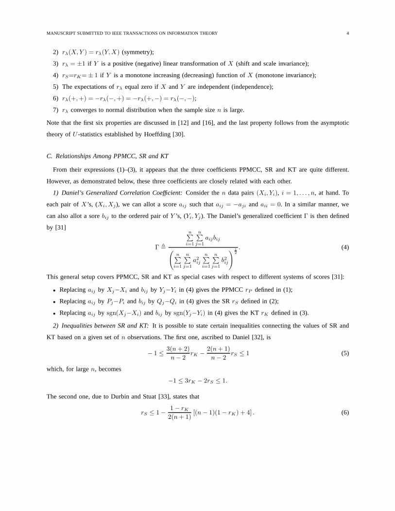
2) rλ(X,Y ) = rλ(Y,X) (symmetry);
3) rλ = ±1 if Y is a positive (negative) linear transformation ofX (shift and scale invariance);
4) rS=rK=± 1 if Y is a monotone increasing (decreasing) function ofX (monotone invariance);
5) The expectations ofrλ equal zero ifX andY are independent (independence);
6) rλ(+,+) = −rλ(−,+) = −rλ(+,−) = rλ(−,−);
7) rλ converges to normal distribution when the sample sizen is large.
Note that the first six properties are discussed in [12] and [16], and the last property follows from the asymptotic
theory ofU -statistics established by Hoeffding [30].
C. Relationships Among PPMCC, SR and KT
From their expressions (1)–(3), it appears that the three coefficients PPMCC, SR and KT are quite different.
However, as demonstrated below, these three coefficients are closely related with each other.
1) Daniel’s Generalized Correlation Coefficient:Consider then data pairs(Xi, Yi), i = 1, . . . , n, at hand. To
each pair ofX ’s, (Xi, Xj), we can allot a scoreaij such thataij = −aji andaii = 0. In a similar manner, we
can also allot a sorebij to the ordered pair ofY ’s, (Yi, Yj). The Daniel’s generalized coefficientΓ is then defined
by [31]
Γ ,
n∑
i=1
n∑
j=1
aijbij
(n∑
i=1
n∑
j=1
a2ijn∑
i=1
n∑
j=1
b2ij
) 1
2
. (4)
This general setup covers PPMCC, SR and KT as special cases with respect to different systems of scores [31]:
• Replacingaij by Xj−Xi andbij by Yj−Yi in (4) gives the PPMCCrP defined in (1);
• Replacingaij by Pj−Pi andbij by Qj−Qi in (4) gives the SRrS defined in (2);
• Replacingaij by sgn(Xj−Xi) andbij by sgn(Yj−Yi) in (4) gives the KTrK defined in (3).
2) Inequalities between SR and KT:It is possible to state certain inequalities connecting thevalues of SR and
KT based on a given set ofn observations. The first one, ascribed to Daniel [32], is
− 1 ≤ 3(n+ 2)
n− 2rK − 2(n+ 1)
n− 2rS ≤ 1 (5)
which, for largen, becomes
−1 ≤ 3rK − 2rS ≤ 1.
The second one, due to Durbin and Stuat [33], states that
rS ≤ 1− 1− rK2(n+ 1)
[(n− 1)(1− rK) + 4] . (6)

MANUSCRIPT SUBMITTED TO IEEE TRANSACTIONS ON INFORMATION THEORY 5
Combing (5) and (6) and lettingn→ ∞ yield the bounds of SR, in terms of KT, as
3
2rK − 1
2≤ rS ≤ 1
2+ rK − 1
2r2K , rK ≥ 0
3
2rK +
1
2≥ rS ≥ 1
2r2K + rK − 1
2, rK ≤ 0.
3) Relationship of SR to Other Coefficients:Besides the PPMCC and KT, SR is also closely related to other
correlation coefficients, e.g., theorder statistics correlation coefficient(OSCC) [34]–[36] and theGini correlation
(GC) [37]. In fact, SR can be reduced from the OSCC and GC by replacing the variates with corresponding
ranks [38].
III. A UXILIARY RESULTS IN NORMAL CASES
In this section we provide some prerequisites concerning the orthant probabilities of normal distributions. These
probabilities, contained in Lemma 1, are critical for the development of Theorem 1 and Theorem 2 later on.
Moreover, some well known results about the expectation andvariance of PPMCC, SR and KT are collected
in Lemma 2 for ease of exposition. For convenience, we use symbols E(N), V(N), C(N,), and corr(N,) in
the sequel to denote the mean, variance, covariance, and correlation of (between) random variables, respectively.
Symbols ofbig oh and little oh are utilized to compare the magnitudes of two functionsu(N) and v(N) as the
argumentN tends to a limitL (might be infinite). The notationu(N) = O(v(N)), N→L, denotes that|u(N)/v(N)|remains bounded asN→L; whereas the notationu(N) = o(v(N)), N→L, denotes thatu(N)/v(N)→0 asN→L [39].
Symbols ofP 0m(Z1, . . . , Zm) are adopted to denote the positive orthant probabilities associated with multivariate
normal random vectors[Z1 · · ·Zm] of dimensionsm = 1, . . . , 4, respectively. The notationR(rs)m×m stands for
correlation matrix with each elementrs , corr(Zr, Zs), r, s = 1, . . . ,m. Obviously the diagonal entries inR are
all unities. For compactness, we will also use the symbolP 0m(R) to denoteP 0
m(Z1, . . . , Zm) in the sequel.
A. Orthant Probabilities for Normal Distributions
Lemma 1:Assume thatZ1, Z2, Z3, Z4 follow a quadrivariate normal distribution with zero meansand correlation
matrix R = (rs)4×4. Define
H(N) ,
1 (N > 0)
0 (N ≤ 0).
(7)

MANUSCRIPT SUBMITTED TO IEEE TRANSACTIONS ON INFORMATION THEORY 6
Then the orthant probabilities
P 01 (Z1) , E H(Z1)
=1
2(8)
P 02 (Z1, Z2) , E H(Z1)H(Z2)
=1
4
(
1 +2
πsin−1 12
)
(9)
P 03 (Z1, Z2, Z3) , E H(Z1)H(Z2)H(Z3)
=1
8
(
1 +2
π
2∑
r=1
3∑
s=r+1
sin−1 rs
)
(10)
P 04 (Z1, Z2, Z3, Z4) , E H(Z1)H(Z2)H(Z3)H(Z4)
=1
16
(
1+2
π
3∑
r=1
4∑
s=r+1
sin−1 rs+W
)
(11)
where
W,1
π4
+∞
−∞
exp(− 1
2zRzT)
z1z2z3z4dz1dz2dz3dz4 (12)
=
4∑
ℓ=2
4
π2
ˆ 1
0
1ℓ
[1−21ℓu2]1
2
sin−1
[αℓ(u)
βℓ(u)γℓ(u)
]
du (13)
with
α2=34−2324−[1314+12(1234−1423−1324)]u2
α3=24−2334−[1214+13(1324−1423−1234)]u2
α4=23−2434−[1213+14(1423−1324−1234)]u2
β2=β3=[1−223−(212+
213−2121323)u
2] 1
2
γ2=β4=[1−224−(212+
214−2121424)u
2] 1
2
γ3=γ4=[1−234−(213+
214−2131434)u
2] 1
2 .
Proof: The first statement (8) is trivial. The second one (9) is usually calledSheppard’s theoremin the literature,
although it was proposed earlier by Stieltjes [40]. The third one (10) is a simple generalization of Sheppard’s theorem
based on the relationship [41]
P 03 =
1
2
[
1−3∑
r=1
P 01 (Zr) +
2∑
r=1
3∑
s=r+1
P 02 (Zr, Zs)
]
.
The last one (11) is due to Childs [42] and is termed theChilds’s reduction formulathroughout.
MANUSCRIPT SUBMITTED TO IEEE TRANSACTIONS ON INFORMATION THEORY 7
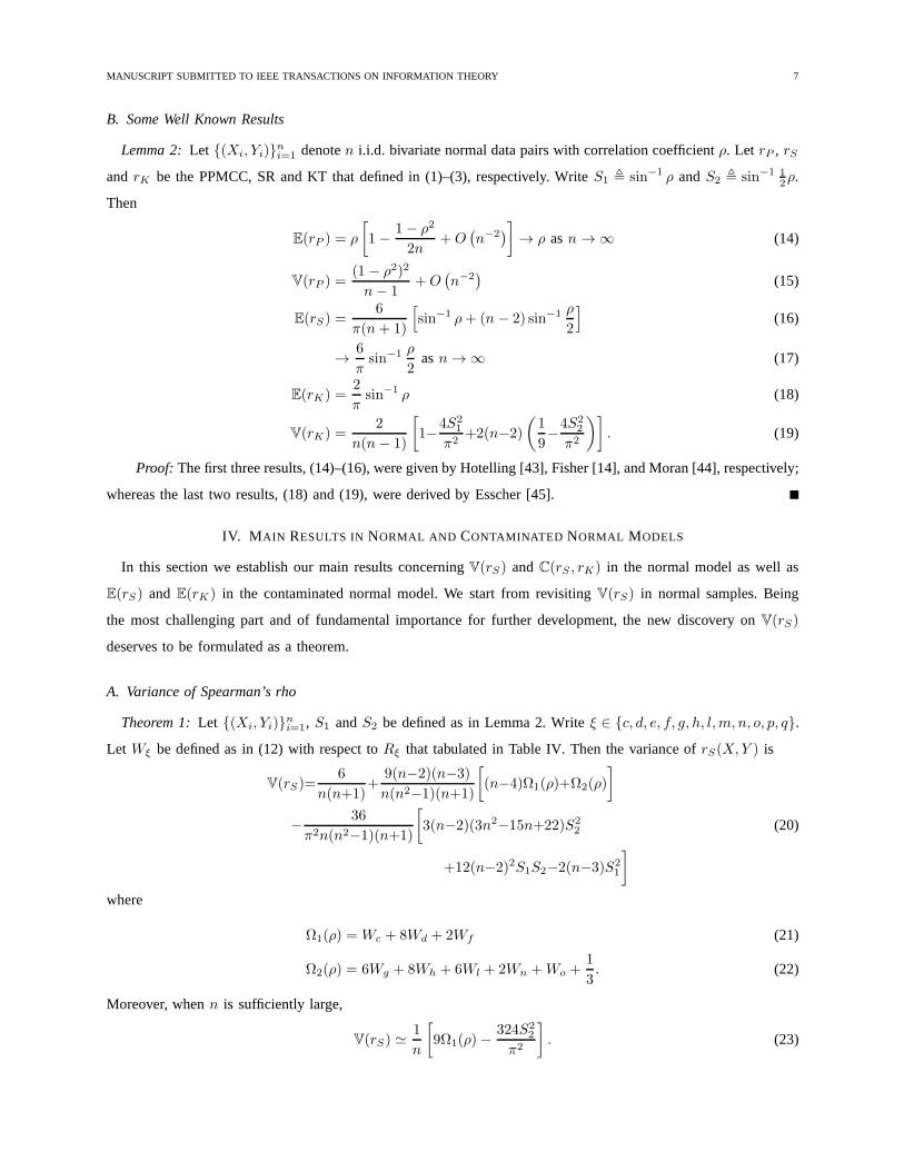
B. Some Well Known Results
Lemma 2:Let (Xi, Yi)ni=1 denoten i.i.d. bivariate normal data pairs with correlation coefficient ρ. Let rP , rS
andrK be the PPMCC, SR and KT that defined in (1)–(3), respectively.Write S1 , sin−1 ρ andS2 , sin−1 12ρ.
Then
E(rP ) = ρ
[
1− 1− ρ2
2n+O
(n−2
)]
→ ρ asn→ ∞ (14)
V(rP ) =(1 − ρ2)2
n− 1+O
(n−2
)(15)
E(rS) =6
π(n+ 1)
[
sin−1 ρ+ (n− 2) sin−1 ρ
2
]
(16)
→ 6
πsin−1 ρ
2asn→ ∞ (17)
E(rK) =2
πsin−1 ρ (18)
V(rK) =2
n(n− 1)
[
1−4S21
π2+2(n−2)
(1
9−4S2
2
π2
)]
. (19)
Proof: The first three results, (14)–(16), were given by Hotelling [43], Fisher [14], and Moran [44], respectively;
whereas the last two results, (18) and (19), were derived by Esscher [45].
IV. M AIN RESULTS IN NORMAL AND CONTAMINATED NORMAL MODELS
In this section we establish our main results concerningV(rS) andC(rS , rK) in the normal model as well as
E(rS) andE(rK) in the contaminated normal model. We start from revisitingV(rS) in normal samples. Being
the most challenging part and of fundamental importance forfurther development, the new discovery onV(rS)
deserves to be formulated as a theorem.
A. Variance of Spearman’s rho
Theorem 1:Let (Xi, Yi)ni=1, S1 andS2 be defined as in Lemma 2. Writeξ ∈ c, d, e, f, g, h, l,m, n, o, p, q.
Let Wξ be defined as in (12) with respect toRξ that tabulated in Table IV. Then the variance ofrS(X,Y ) is
V(rS)=6
n(n+1)+
9(n−2)(n−3)
n(n2−1)(n+1)
[
(n−4)Ω1(ρ)+Ω2(ρ)
]
− 36
π2n(n2−1)(n+1)
[
3(n−2)(3n2−15n+22)S22
+12(n−2)2S1S2−2(n−3)S21
]
(20)
where
Ω1(ρ) =Wc + 8Wd + 2Wf (21)
Ω2(ρ) = 6Wg + 8Wh + 6Wl + 2Wn +Wo +1
3. (22)
Moreover, whenn is sufficiently large,
V(rS) ≃1
n
[
9Ω1(ρ)−324S2
2
π2
]
. (23)
MANUSCRIPT SUBMITTED TO IEEE TRANSACTIONS ON INFORMATION THEORY 8
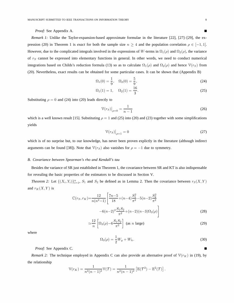
Proof: See Appendix A.
Remark 1:Unlike the Taylor-expansion-based approximate formulae in the literature [22], [27]–[29], the ex-
pression (20) in Theorem 1 isexact for both the sample sizen ≥ 4 and the population correlationρ ∈ [−1, 1].
However, due to the complicated integrals involved in the expressions ofW -terms inΩ1(ρ) andΩ2(ρ), the variance
of rS cannot be expressed into elementary functions in general. In other words, we need to conduct numerical
integrations based on Childs’s reduction formula (13) so asto calculateΩ1(ρ) andΩ2(ρ) and henceV(rS) from
(20). Nevertheless, exact results can be obtained for some particular cases. It can be shown that (Appendix B)
Ω1(0) =1
9, Ω2(0) =
5
9, (24)
Ω1(1) = 1, Ω2(1) =16
3. (25)
Substitutingρ = 0 and (24) into (20) leads directly to
V(rS)∣∣ρ=0
=1
n− 1(26)
which is a well known result [15]. Substitutingρ = 1 and (25) into (20) and (23) together with some simplifications
yields
V(rS)∣∣ρ=1
= 0 (27)
which is of no surprise but, to our knowledge, has never been proven explictly in the literature (although indirect
arguments can be found [38]). Note thatV(rS) also vanishes forρ = −1 due to symmetry.
B. Covariance between Spearman’s rho and Kendall’s tau
Besides the variance of SR just established in Theorem 1, thecovariance between SR and KT is also indispensable
for revealing the basic properties of the estimators to be discussed in Section V.
Theorem 2:Let (Xi, Yi)ni=1, S1 andS2 be defined as in Lemma 2. Then the covariance betweenrS(X,Y )
andrK(X,Y ) is
C(rS , rK)=12
n(n2−1)
[
7n−5
18+(n−4)
S21
π2−5(n−2)
S22
π2
−6(n−2)2S1S2
π2+(n−2)(n−3)Ω3(ρ)
]
(28)
≃12
n
[
Ω3(ρ)−6S1S2
π2
]
(asn large) (29)
where
Ω3(ρ) =1
2Wg +Wh. (30)
Proof: See Appendix C.
Remark 2:The technique employed in Appendix C can also provide an alternative proof ofV(rK) in (19), by
the relationship
V(rK) =1
n2(n− 1)2V(T ) =
1
n2(n− 1)2[E(T 2)− E
2(T )].

MANUSCRIPT SUBMITTED TO IEEE TRANSACTIONS ON INFORMATION THEORY 9
The interested reader, after trying this, will find that the proof by this way is much simpler than the characteristic-
function-based argument detailed in [15].
Corollary 1: In Theorem 2, the covarianceC(rS , rK) can also be expressed as
C(rS , rK)=12
n(n2−1)
[
(n+1)2
18+(n−4)
S21
π2−5(n−2)
S22
π2
−6(n−2)2S1S2
π2+
2
π2(n−2)(n−3)Ω4(ρ)
]
(31)
≃12
n
[1
18+2
Ω4(ρ)
π2−6
S1S2
π2
]
(asn large) (32)
where
Ω4(ρ) =
ˆ ρ
0
[
sin−1(x
3
)
+ 2 sin−1
(x√3
)]dx√1− x2
−2
ˆ ρ
0
sin−1
(
x
2
√
1− x2
9− 3x2
)
dx√4− x2
+
ˆ ρ
0
sin−1
(x
2
5− x2
3− x2
)dx√4− x2
−2
ˆ ρ
0
sin−1
(
x
√
1− x2
12− 6x2
)
dx√4− x2
+2
ˆ ρ
0
sin−1
(
x
√
3− x2
4− 2x2
)
dx√4− x2
.
(33)
Proof: Inverting (11) yields
W = 16P 04 − 1− 2
π
3∑
r=1
4∑
s=r+1
sin−1 rs. (34)
Combining (30) and (34),Ω3(ρ) can be rewritten in terms ofP 04 and the correlation coefficients corresponding to
Rg andRh in Appendix 2 of [29]. This leads to
Ω3(ρ) =1
18+
2
π2Ω4(ρ). (35)
The corollary thus follows directly by substituting (35) to(28) and (29), respectively.
Remark 3:Both (28) and (31) areexact for any value ofn ≥ 4 and |ρ| ≤ 1. However, they are of different
usefulness according to different numerical and analytical purposes. Formula (28) is more convenient in the sence
of controlling the precision of numerical integrations when programming; whereas (31) is more convenient in the
sence of evaluating any order (≥ 1) of derivatives ofC(rS , rK) with respect toρ. These higher order derivatives are
mandatory when expandingC(rS , rK) as a power series inρ, a conventional practice in the literature. For example,
performing the Taylor expansion to (32) with the assistanceof (33) gives
C(rS , rK) ≃ 2
3n
(1− 1.24858961ρ2 + 0.06830496ρ4
+ 0.07280482ρ6 + 0.04025528ρ8 + 0.02189277ρ10 + · · ·)
(36)
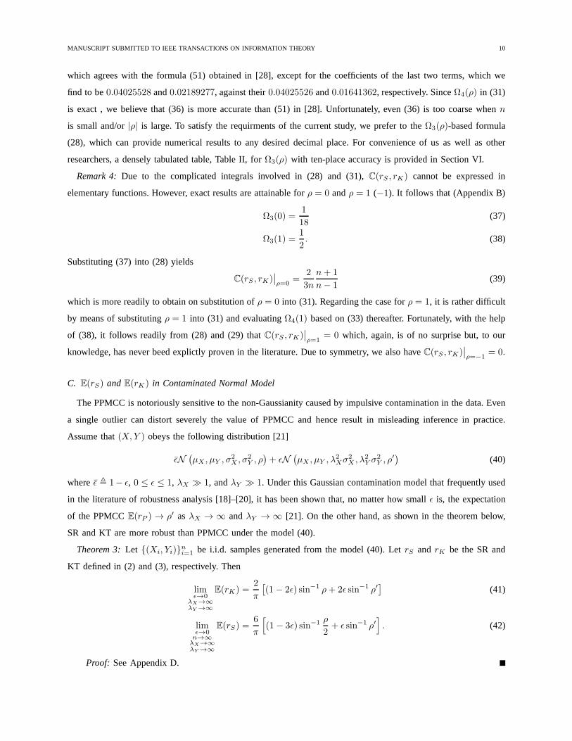
MANUSCRIPT SUBMITTED TO IEEE TRANSACTIONS ON INFORMATION THEORY 10
which agrees with the formula (51) obtained in [28], except for the coefficients of the last two terms, which we
find to be0.04025528 and0.02189277, against their0.04025526 and0.01641362, respectively. SinceΩ4(ρ) in (31)
is exact , we believe that (36) is more accurate than (51) in [28]. Unfortunately, even (36) is too coarse whenn
is small and/or|ρ| is large. To satisfy the requirments of the current study, weprefer to theΩ3(ρ)-based formula
(28), which can provide numerical results to any desired decimal place. For convenience of us as well as other
researchers, a densely tabulated table, Table II, forΩ3(ρ) with ten-place accuracy is provided in Section VI.
Remark 4:Due to the complicated integrals involved in (28) and (31),C(rS , rK) cannot be expressed in
elementary functions. However, exact results are attainable for ρ = 0 andρ = 1 (−1). It follows that (Appendix B)
Ω3(0) =1
18(37)
Ω3(1) =1
2. (38)
Substituting (37) into (28) yields
C(rS , rK)∣∣ρ=0
=2
3n
n+ 1
n− 1(39)
which is more readily to obtain on substitution ofρ = 0 into (31). Regarding the case forρ = 1, it is rather difficult
by means of substitutingρ = 1 into (31) and evaluatingΩ4(1) based on (33) thereafter. Fortunately, with the help
of (38), it follows readily from (28) and (29) thatC(rS , rK)∣∣ρ=1
= 0 which, again, is of no surprise but, to our
knowledge, has never beed explictly proven in the literature. Due to symmetry, we also haveC(rS , rK)∣∣ρ=−1
= 0.
C. E(rS) andE(rK) in Contaminated Normal Model
The PPMCC is notoriously sensitive to the non-Gaussianity caused by impulsive contamination in the data. Even
a single outlier can distort severely the value of PPMCC and hence result in misleading inference in practice.
Assume that(X,Y ) obeys the following distribution [21]
ǫN(µX , µY , σ
2X , σ
2Y , ρ
)+ ǫN
(µX , µY , λ
2Xσ
2X , λ
2Y σ
2Y , ρ
′)
(40)
whereǫ , 1− ǫ, 0 ≤ ǫ ≤ 1, λX ≫ 1, andλY ≫ 1. Under this Gaussian contamination model that frequently used
in the literature of robustness analysis [18]–[20], it has been shown that, no matter how smallǫ is, the expectation
of the PPMCCE(rP ) → ρ′ asλX → ∞ andλY → ∞ [21]. On the other hand, as shown in the theorem below,
SR and KT are more robust than PPMCC under the model (40).
Theorem 3:Let (Xi, Yi)ni=1 be i.i.d. samples generated from the model (40). LetrS and rK be the SR and
KT defined in (2) and (3), respectively. Then
limǫ→0
λX→∞λY →∞
E(rK) =2
π
[(1 − 2ǫ) sin−1 ρ+ 2ǫ sin−1 ρ′
](41)
limǫ→0n→∞λX→∞λY →∞
E(rS) =6
π
[
(1− 3ǫ) sin−1 ρ
2+ ǫ sin−1 ρ′
]
. (42)
Proof: See Appendix D.

MANUSCRIPT SUBMITTED TO IEEE TRANSACTIONS ON INFORMATION THEORY 11
Remark 5: It was stated without substantial argument in [21] that, under the model (40),E(rS) is of the following
form
E(rS) =6
π
[
(1− ǫ) sin−1 ρ
2+ ǫ sin−1 ρ
′
2
]
(∗)
as ǫ → 0, λX → ∞ andλY → ∞. This is quite inconsistent with our result (42) in Theorem 3. We will resolve
the controversy between (42) and (∗) by Monte Carlo simulations in Section VI.
V. ESTIMATORS OF THEPOPULATION CORRELATION
In this section, we investigate the performance of the estimators ofρ based on SR and KT in terms of bias, MSE
and ARE to PPMCC. To gain further insight into their relationship, the correlation between the two estimatorsρS
and ρK (defined below) is also derived.
A. Asymptotic Unbiased Estimators
Inverting (14), (17) and (18), we have the following estimators of ρ
ρP , rP (43)
ρS , 2 sin(π
6rS
)
(44)
ρK , sin(π
2rK
)
. (45)
Moreover, another estimator based on a mixture ofrS andrP can be constructed as [15]
ρM , 2 sin
(π
6rS − π
2
rK − rSn− 2
)
(46)
based on the following relationship
E(rS) =6
π
(
S2 +S1 − 3S2
n+ 1
)
. (47)
In the sequel we will focus on the properties of the estimators defined in (43)–(46). Here the estimatorρP in (43)
is employed as a benchmark due to its optimality for normal samples, in the sense of approaching the CRLB [11]
when the sample size is sufficiently large.
B. Bias Effect for Small Samples
It is noteworthy that the four estimators in (43)–(46) are unbiased only for large samples. When the sample size
is small, the bias effects, as shown in the following theorem, are not ignorable any more.
Theorem 4:Let ρζ , ζ ∈ P, S,K,M be defined as in (43)–(46), respectively. DefineBIASζ , E(ρζ − ρ). Let
S1 andS2 bear the same meanings as in Lemma 2. Writeσ2S , V(rS), σ2
K , V(rK) and σS,K , C(rS , rK).

MANUSCRIPT SUBMITTED TO IEEE TRANSACTIONS ON INFORMATION THEORY 12
Then, under the same assumptions made as in Theorem 1,
BIASP ≃ − 1
2nρ(1− ρ2) (48)
BIASS ≃√
4− ρ2
n+ 1(S1 − 3S2)−
π2ρ
72σ2S (49)
BIASK ≃ −π2ρ
8σ2K (50)
BIASM ≃ − 1
72
π2ρ
(n−2)2[(n+1)2σ2
S−6(n+1)σS,K+9σ2K
]. (51)
Proof: The first statement (48) follows directly from (14) in Lemma 2. Now we proceed to evaluateBIASS ,
BIASK and BIASM . For convenience, writerS,E(rS), rK,E(rK), δS,rS−rS , and δK,rK−rK . Expanding
(44) aroundrS yields
ρS=2 sin(π
6rS
)
+π
3cos(π
6rS
)
δS−π2
36sin(π
6rS
)
δ2S+ · · · . (52)
Taking expectation of both sides in (52), applyingE(δS) = 0, E(δ2S) = σ2S and ignoring the high order infinitesimals,
we have
E(ρS) ≃ 2 sin(π
6rS
)
− π2
36sin(π
6rS
)
σ2S . (53)
Substituting (47) into (53), expanding to the order of(n+ 1)−1, and subtractingρ thereafter, we obtain the result
(49). In a similar way we have
E(ρK) ≃ ρ− π2ρ
8σ2K
which leads directly to (50). Performing Taylor expansion of ρM (rS , rK) around(rS , rK) till the second order, we
have
ρM = ρM (rS , rK) +∂(ρM )
∂(rS)δS +
∂(ρM )
∂(rK)δK
+1
2
[∂2(ρM )
∂(rS)2δ2S+
∂2(ρM )
∂(rK)2δ2K+
2∂2(ρM )δSδK∂(rS)∂(rK)
]
+ · · · .(54)
Taking expectation of both sides in (54), ignoring high order infinitesimals, applying the resultsρM (rS , rK) = ρ,
E(δS) = 0, E(δK) = 0, E(δ2S) = σ2S , E(δ2K) = σ2
K , E(δS , δK) = σS,K along with the second order partial
derivatives
∂2ρM (rS , rK)
∂(rS)2= −π
2ρ
36
(n+ 1)2
(n− 2)2
∂2ρM (rS , rK)
∂(rK)2= −π
2ρ
4
1
(n− 2)2
∂2ρM (rS , rK)
∂(rS)∂(rK)=π2ρ
12
n+ 1
(n− 2)2
and subtractingρ thereafter, we arrive at the forth theorem statement (51), thus completing the proof.
Remark 6:From (48)–(51), it follows that, for all the four estimators,
• BIASζ(ρ) = BIASζ(−ρ) (odd symmetry);
• ρBIASζ(ρ) ≤ 0 (negative bias);

MANUSCRIPT SUBMITTED TO IEEE TRANSACTIONS ON INFORMATION THEORY 13
• BIASζ = 0 for ρ ∈ −1, 0, 1;
• BIASζ ∼ O(n−1) asn→ ∞.
Moreover, contrary toBIASP andBIASK , BIASS andBIASM cannot be expressed into elementary functions due
to the intractability involved in (20) and (28), the expressions ofV(rS) andC(rS , rK), respectively.
C. Approximation of Variances
Besides the bias effect just discussed, the variance is another importantfigure of meritwhen comparing the
performance of the estimatorsρζ , ζ ∈ P, S,K,M. From (14), it follows that
V(ρP ) ≃(1− ρ2)2
n− 1. (55)
By the delta method, it follows that [15]
V(ρS) ≃π2(4 − ρ2)
36V(rS) (56)
V(ρK) ≃ π2(1 − ρ2)
4V(rK). (57)
Now we only need to deal withV(ρM ), which is stated below.
Theorem 5:Let ρM be defined as in (46). Then, under the same assumptions made asin Theorem 1,
V(ρM ) ≃ π2(4− ρ2)
36(n− 2)2[(n+ 1)2σ2
S − 6(n+ 1)σS,K + 9σ2K
]. (58)
Proof: Using the delta method [11], it follows that
V(ρM )≃[∂(ρM )
∂(rS)
]2
σ2S+
[∂(ρM )
∂(rK)
]2
σ2K+2
∂(ρM )
∂(rS)
∂(ρM )
∂(rK)σS,K . (59)
The theorem thus follows with substitutions of the partial derivatives
∂ρM (rS , rK)
∂(rS)=π
6
n+ 1
n− 2
√
4− ρ2
∂ρM (rS , rK)
∂(rK)=π
2
−1
n− 2
√
4− ρ2
into (59), respectively.
D. Asymptotic Relative Efficiency
Thus far in this section we have established the analytical results with an emphasis on limited-sized bivariate
normal samples. For a better understanding of the fourt estimators, we will shift our attention to the asymptotic
properties ofρζ in the sequel. Sincelimn→∞ E(ρζ) = ρ, we can compare their performances by means of the
asymptotic relative efficiency, which is defined as [11]
AREζ , limn→∞
V(ρP )
V(ρζ), ζ ∈ P, S,K,M. (60)
As remarked before, we employρP as a benchmark, since, for large-sized bivariate normal samples,ρP approaches
the Cramer-Rao lower bound (CRLB) [11]
CRLB =(1− ρ2)2
n. (61)

MANUSCRIPT SUBMITTED TO IEEE TRANSACTIONS ON INFORMATION THEORY 14
From (60) it is obvious thatAREP = 1. Moreover, comparing (56) and (58), it is easily seen thatlimn→∞ V(ρS)/V(ρM ) =
1, which leads readily toARES = AREM by referring to (60). Then we only need to focus onARES andAREK
in the following discussion.
Theorem 6:Let ARES andAREK be defined as in (60). Then
ARES =36(1− ρ2)2
(4 − ρ2)[
9π2Ω1(ρ)− 324(sin−1 1
2ρ)2] (62)
AREK =9(1− ρ2)
π2 − 36(sin−1 1
2ρ)2 . (63)
Proof: Substituting (56) and (57) into (60) yields (62) and (63), respectively, and the proof completes.
Remark 7:Due to the intractability ofΩ1(ρ) in (62), ARES cannot be expressed into elementary functions in
general. However, exact results are obtainable forρ = 0,±1. Substitutingρ = 0 andΩ1(0) = 1/9 into (62), it is
easy to verify that
ARES(0) =9
π2≃ 0.9119
which is a well known result [15]. In our previous work [38] wealso obtained that
ARES(±1) =15 + 11
√5
57≃ 0.6947. (64)
Now let us investigateAREK . It follows from (63) that,AREK is expressible as elementary functions ofρ, and
is therefore more tractable thanARES . In other words, we can evaluate easily any value ofAREK with respect
to any value ofρ 6= ±1. For example, substitutingρ = 0 into (63) yields
AREK(0) =9
π2
which is identical toARES(0) and also well known [15]. However, whenρ → ±1, an extra effort is necessary,
since both the numerator and denominator of (63) vanish in this case. Apply the L’Hopital’s rule, we find the
following result
AREK
∣∣ρ→±1
=1
4
ρ√
4− ρ2
sin−1 12ρ
∣∣∣∣∣ρ=±1
=3√3
2π≃ 0.8270 (65)
which is greater thanARES(±1). In fact, a comparison ofARES andAREK in Section VI suggest thatARES ≤AREK for all ρ ∈ [−1, 1].
VI. N UMERICAL RESULTS
In this section we aim at 1) tabulating the values ofΩ1(ρ), Ω2(ρ) (in Theorem 1) andΩ3(ρ) (in Theorem 2)
that are not expressible as elementary functions, 2) verifying the theoretical results Theorems 1 to 6 established in
previous sections, and 3) comparing the performances of thefour estimators defined in (43)–(46) by means ofbias
effect, mean square error(MSE) and ARE under both the normal and contaminated normal models. Throughout this
section, Monte Carlo experiments are undertaken for10 ≤ n ≤ 100. A sample size ofn = 1000 is considered large
enough when we investigate the asymptotic behaviors. The number of trials is set to5×105 for reason of accuracy.

MANUSCRIPT SUBMITTED TO IEEE TRANSACTIONS ON INFORMATION THEORY 15
TABLE I
VALUES OFΩ1(ρ) AND Ω2(ρ) IN THEOREM 1
.ρ 0.00+ 0.10+ 0.20+ 0.30+ 0.40+ 0.50+ 0.60+ 0.70+ 0.80+ 0.90+
0.00 0.1111111111 0.1185038469 0.1408155407 0.1784569533 0.2321489296 0.3029841008 0.3925307865 0.5030051934 0.6375648509 0.80084018540.01 0.1111849294 0.1200591282 0.1438805317 0.1830890232 0.2384392872 0.3110659830 0.4025930108 0.5153148070 0.6525067154 0.81899179290.02 0.1114063976 0.1217636535 0.1470991369 0.1878822020 0.2449020129 0.3193363285 0.4128663989 0.5278679000 0.6677394272 0.83750749570.03 0.1117755552 0.1236177309 0.1504719575 0.1928374325 0.2515384762 0.3277970726 0.4233536847 0.5406684104 0.6832688919 0.85639678830.04 0.1122924682 0.1256216966 0.1539996256 0.1979556956 0.2583500955 0.3364502180 0.4340577002 0.5537204299 0.6991012791 0.87566968200.05 0.1129572289 0.1277759147 0.1576828058 0.2032380114 0.2653383401 0.3452978372 0.4449813799 0.5670282120 0.7152430387 0.89533674680.06 0.1137699564 0.1300807778 0.1615221950 0.2086854397 0.2725047311 0.3543420748 0.4561277650 0.5805961801 0.7317009189 0.91540915740.07 0.1147307963 0.1325367071 0.1655185233 0.2142990814 0.2798508436 0.3635851506 0.4675000084 0.5944289365 0.7484819855 0.93589874500.08 0.1158399207 0.1351441527 0.1696725544 0.2200800791 0.2873783079 0.3730293618 0.4791013791 0.6085312723 0.7655936432 0.95681805540.09 0.1170975289 0.1379035942 0.1739850867 0.2260296186 0.2950888115 0.3826770865 0.4909352680 0.6229081771 0.7830436585 0.9781804140
0.00 0.55555555560.58317791990.66694115480.80965487281.01644699671.29560504341.66024280052.13183984402.74909613533.59880678900.01 0.55583105250.58899736380.67849522700.82734234441.04093531981.32795007271.70213069472.18613344712.82136872973.70414281940.02 0.55665763120.59537855320.69064087590.84567465651.06615387171.36115991881.74510312812.24190452302.89597179333.81489648000.03 0.55803555470.60232356370.70338227250.86465870571.09211350541.39525186081.78918931592.29920921212.97304750223.93187740050.04 0.55996526240.60983466290.71672382500.88430171531.11882557601.43024404451.83442021992.35810812953.05275625964.05616983330.05 0.56244736980.61791431370.73067018490.90461124801.14630196521.46615553841.88082869622.41866690283.13528041124.18929495030.06 0.56548266980.62656517760.74522625440.92559521941.17455510901.50300639441.92844966032.48095680213.22082904184.33352668160.07 0.56907213340.63579011830.76039719350.94726191271.20359802651.54081771411.97732027242.54505548073.30964427384.49259130450.08 0.57321691150.64559220550.77618842850.96961999361.23344435181.57961172192.02748014602.61104785263.40200969994.67355717040.09 0.57791833550.65597471930.79260566020.99267852751.26410836791.61941184482.07897158362.67902714033.49826192704.8941554764
(a) In the upper panel are the values ofΩ1(ρ), and in the lower panel (shaded area) are the values ofΩ2(ρ);(b) Ω1(0) = 1/9, Ω1(1) = 1, Ω1(−ρ) = Ω1(ρ);(c) Ω2(0) = 5/9, Ω2(1) = 16/3, Ω2(−ρ) = Ω2(ρ).
TABLE II
VALUES OFΩ3(ρ) IN THEOREM2
ρ 0.00+ 0.10+ 0.20+ 0.30+ 0.40+ 0.50+ 0.60+ 0.70+ 0.80+ 0.90+
0.00 0.0555555556 0.0579082728 0.0650488362 0.0772363477 0.0949464623 0.1189551518 0.1505074640 0.1916842312 0.2463473665 0.32356865230.01 0.0555790160 0.0584040661 0.0660345125 0.0787487694 0.0970477974 0.1217448819 0.1541471283 0.1964547749 0.2528155359 0.33335725180.02 0.0556494053 0.0589477686 0.0670708481 0.0803167902 0.0992127259 0.1246109820 0.1578844390 0.2013621185 0.2595091876 0.34371450880.03 0.0557667477 0.0595395710 0.0681582284 0.0819410523 0.1014422703 0.1275551071 0.1617222612 0.2064119567 0.2664434835 0.35473349720.04 0.0559310834 0.0601796821 0.0692970610 0.0836222291 0.1037375018 0.1305789987 0.1656636397 0.2116104637 0.2736356357 0.36654001660.05 0.0561424692 0.0608683287 0.0704877763 0.0853610263 0.1060995431 0.1336844907 0.1697118152 0.2169643536 0.2811053381 0.37931225560.06 0.0564009777 0.0616057558 0.0717308284 0.0871581833 0.1085295710 0.1368735157 0.1738702420 0.2224809499 0.2888753252 0.39331922580.07 0.0567066983 0.0623922274 0.0730266953 0.0890144747 0.1110288192 0.1401481121 0.1781426083 0.2281682700 0.2969721099 0.40900628490.08 0.0570597366 0.0632280263 0.0743758804 0.0909307119 0.1135985821 0.1435104314 0.1825328587 0.2340351233 0.3054269741 0.42722723920.09 0.0574602150 0.0641134550 0.0757789125 0.0929077445 0.1162402177 0.1469627471 0.1870452202 0.2400912305 0.3142773322 0.4501481060
Note that (a)Ω3(0) = 1/18, (b) Ω3(1) = 1/2, and (c)Ω3(−ρ) = Ω3(ρ).
All samples are generated by functions in the MatlabStatistics ToolboxTM. Specifically, the normal samples
are generated bymvnrnd, whereas the contaminated normal samples are generated bygmdistribution and
random. The notationρ = ρ1(∆ρ)ρ2 represents a list ofρ starting fromρ1 to ρ2 with increment∆ρ.
A. Tables ofΩ1(ρ), Ω2(ρ) andΩ3(ρ)
Table I contains the values ofΩ1(ρ) andΩ2(ρ) in (20), the first statement of Theorem 1 forρ = 0(0.01)1. In
the upper panel are the values ofΩ1(ρ); whereas in the lower panel are the values ofΩ2(ρ). Due to the importance
MANUSCRIPT SUBMITTED TO IEEE TRANSACTIONS ON INFORMATION THEORY 16
−1.0 −0.5 0.0 0.5 1.0
−5.0
0.0
5.0
·10−2
ρ
BIA
Sζ
(a) n = 10
BIASTP BIAST
S BIASTK BIAST
M
BIASOP BIASO
S BIASOK BIASO
M
−1.0 −0.5 0.0 0.5 1.0
−2.0
0.0
2.0
·10−2
ρ
(b) n = 20
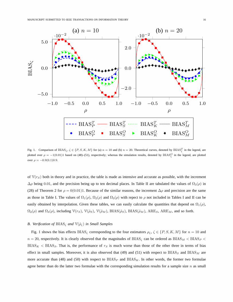
Fig. 1. Comparison ofBIASζ , ζ ∈ P, S,K,M for (a) n = 10 and (b)n = 20. Theoretical curves, denoted byBIASTζ in the legend, are
plotted overρ = −1(0.01)1 based on (48)–(51), respectively; whereas the simulation results, denoted byBIASOζ in the legend, are plotted
over ρ = −0.9(0.1)0.9.
of V(rS) both in theory and in practice, the table is made as intensiveand accurate as possible, with the increment
∆ρ being0.01, and the precision being up to ten decimal places. In Table IIare tabulated the values ofΩ3(ρ) in
(28) of Theorem 2 forρ = 0(0.01)1. Because of the similar reasons, the increment∆ρ and precision are the same
as those in Table I. The values ofΩ1(ρ), Ω2(ρ) andΩ3(ρ) with repect toρ not included in Tables I and II can be
easily obtained by interpolation. Given these tables, we can easily calculate the quantities that depend onΩ1(ρ),
Ω2(ρ) andΩ3(ρ), includingV(rS), V(ρS), V(ρM ), BIAS(ρS), BIAS(ρM ), ARES , AREM , and so forth.
B. Verification ofBIASζ andV(ρζ) in Small Samples
Fig. 1 shows the bias effectsBIASζ corresponding to the four estimatorsρζ , ζ ∈ P, S,K,M for n = 10 and
n = 20, respectively. It is clearly observed that the magnitudes of BIASζ can be ordered asBIASM < BIASP <
BIASK < BIASS . That is, the performance ofrS is much worse than those of the other three in terms of bias
effect in small samples. Moreover, it is also observed that (49) and (51) with respect toBIASS andBIASM are
more accurate than (48) and (50) with respect toBIASP andBIASK . In other words, the former two formulae
agree better than do the latter two formulae with the corresponding simulation results for a sample sizen as small

MANUSCRIPT SUBMITTED TO IEEE TRANSACTIONS ON INFORMATION THEORY 17
−1.0 −0.5 0.0 0.5 1.0
0.000
0.050
0.100
0.150
MSE
ζ(a) n = 10
MSEP
MSES
MSEK
MSEM
−1.0 −0.5 0.0 0.5 1.0
0.000
0.020
0.040
0.060
(b) n = 20
MSEP
MSES
MSEK
MSEM
−1.0 −0.5 0.0 0.5 1.0
0.000
0.010
0.020
0.030
ρ
MSE
ζ
(c) n = 40
MSEP
MSES
MSEK
MSEM
−1.0 −0.5 0.0 0.5 1.0
0.000
0.005
0.010
0.015
0.020
ρ
(d) n = 60
MSEP
MSES
MSEK
MSEM
Fig. 2. Comparison of observedMSEζ , ζ ∈ P, S,K,M for (a) n = 10, (b) n = 20, (c) n = 40, and (d)n = 60 over ρ = −1(0.1)1,
respectively.
as 10. Nevertheless, the deviations from (48) and (50) to the corresponding simulation results are less noticeable
when the sample sizen is increased up to20.
Table III lists, for each of the three samples sizes,10, 20 and30, 1) the theoretical results (55)–(58) with respect
to V(ρζ) and 2) the corresponding observed variances from the Monte Carlo simulations. It can be seen that (56)
and (58), with respect toV(ρS) andV(ρM ), are accurate enough even though the sample size is as small asn = 10.
On the other hand, unfortunately, the theoretical formula (55) for V(ρP ) and (57) forV(ρK) deviate substantially
from the corresponding observed simulation results for thesame sample sizen = 10. However, it appears that
these deviations become less noticeable forn = 20 and negligible forn = 30. Therefore, it would be save to use

MANUSCRIPT SUBMITTED TO IEEE TRANSACTIONS ON INFORMATION THEORY 18
0.00 0.10 0.20 0.30 0.40 0.50 0.60 0.70 0.80 0.90 1.00
0.70
0.75
0.80
0.85
0.90
ρ
Asy
mpt
otic
Rel
ativ
eE
ffici
ency
Theory:ARES
Theory:AREK
Observed:ARES
Observed:AREK
Fig. 3. Verification and Comparison ofARES andAREK for n = 1000 over ρ = 0(0.01)1, for theoretical curves, andρ = 0(0.05)0.95,
for simulation results. The results (64) and (65) are used toplot the two theoretical curves forρ = 1, respectively.
TABLE III
VARIANCES OFV(ρζ ), ζ ∈ P, S,K,M FORn = 10, 20, 30
Sample sizen = 10 Sample sizen = 20 Sample sizen = 30
V(ρP ) V(ρS) V(ρK) V(ρM ) V(ρP ) V(ρS) V(ρK ) V(ρM ) V(ρP ) V(ρS) V(ρK) V(ρM )
ρ (53) Obs. (54) Obs. (55) Obs. (56) Obs. (53) Obs. (54) Obs. (55) Obs. (56) Obs. (53) Obs. (54) Obs. (55) Obs. (56) Obs.
0.0 0.111 0.111 0.122 0.119 0.152 0.133 0.148 0.143 0.053 0.053 0.058 0.057 0.065 0.061 0.064 0.063 0.034 0.034 0.038 0.037 0.041 0.039 0.040 0.0400.1 0.109 0.109 0.120 0.117 0.150 0.131 0.145 0.141 0.052 0.052 0.057 0.056 0.064 0.060 0.063 0.062 0.034 0.034 0.037 0.037 0.040 0.039 0.040 0.0390.2 0.102 0.105 0.115 0.112 0.142 0.125 0.138 0.135 0.049 0.049 0.054 0.054 0.060 0.057 0.059 0.059 0.032 0.032 0.035 0.035 0.038 0.037 0.038 0.0370.3 0.092 0.096 0.106 0.105 0.129 0.117 0.127 0.125 0.044 0.045 0.049 0.049 0.055 0.052 0.054 0.054 0.029 0.029 0.032 0.032 0.034 0.034 0.034 0.0340.4 0.078 0.085 0.094 0.094 0.113 0.104 0.112 0.111 0.037 0.039 0.043 0.043 0.047 0.046 0.047 0.047 0.024 0.025 0.028 0.028 0.030 0.029 0.030 0.0300.5 0.063 0.071 0.080 0.081 0.093 0.089 0.093 0.094 0.030 0.032 0.036 0.036 0.039 0.038 0.039 0.039 0.019 0.020 0.023 0.023 0.024 0.024 0.024 0.0250.6 0.046 0.055 0.063 0.065 0.070 0.071 0.073 0.074 0.022 0.024 0.028 0.028 0.029 0.029 0.030 0.030 0.014 0.015 0.018 0.018 0.018 0.018 0.019 0.0190.7 0.029 0.038 0.046 0.048 0.048 0.052 0.051 0.053 0.014 0.016 0.019 0.020 0.019 0.020 0.020 0.021 0.009 0.010 0.012 0.012 0.012 0.012 0.012 0.0130.8 0.014 0.021 0.028 0.030 0.026 0.031 0.029 0.031 0.007 0.008 0.011 0.011 0.010 0.011 0.011 0.011 0.004 0.005 0.007 0.007 0.006 0.007 0.007 0.0070.9 0.004 0.007 0.012 0.013 0.009 0.012 0.011 0.012 0.002 0.002 0.004 0.004 0.003 0.004 0.004 0.004 0.001 0.001 0.002 0.002 0.002 0.002 0.002 0.002

MANUSCRIPT SUBMITTED TO IEEE TRANSACTIONS ON INFORMATION THEORY 19
(55)–(58) when approximating the variances ofρζ for n ≥ 20 in practice.
C. Comparison of MSE in Small Samples
Contrary toBIASζ illustrated in Fig. 1, the magnitudes of the mean square errors
MSEζ , E[(ρζ − ρ)2
], ζ ∈ P, S,K,M
cannot be ordered in a consistent manner. It appears in Fig. 2that 1)MSEM > MSEK > MSES > MSEP when
|ρ| is around0, 2) MSES > MSEK > MSEP when |ρ| exceeds some threshold, which moves towards0 with
increase ofn, and 3) the difference betweenMSEK andMSES aroundρ = 0 decreases steadily with increase of
n. Furthermore, due to the asymptotic equivalence betweenρS and ρM , MSES andMSEM becomes closer and
closer asn increases.
D. Verification and Comparison ofARES andAREK
Fig. 3 verifies and compares the performance ofρS andρK in terms of ARE. For purpose of numerical verification,
simulation results forn = 1000 are superimposed upon the corresponding theoretical curves. Due to the asymptotic
equivalence betweenρS andρM , the results with respect toAREM are not included in Fig. 3. It can be observed that
1) the simulations agree well with our theoretical findings in (62) and (63), respectively, 2)AREK lies consistently
aboveARES , indicating the superiority ofρK over ρS for large samples, and 3) the performance ofρS deteriorates
severely asρ approaching unity, although it performs similarly asρK whenρ is small. Note that the remarks on
ARES also apply toAREM due to the equivalence betweenρS and ρM when the sample sizen is large.
E. Performance ofρζ in Contaminated Normal Model
Fig. 4 puports to 1) verify the two statements concerningE(rK) andE(rS) in Theorem 3 under the contaminated
Gaussian model (40), and 2) compare our formula (42) with theresult of (∗) that asserted in [21]. Due to the lack
of space, we only present the results forǫ = 0.01 andǫ = 0.05 under the sample sizen = 50 here. For simplicity,
the rest parameters of the model (40) are set to beσX = σY = 1, λX = λY = 100 andρ′ = 0 throughout. It is
seen that the observed values ofE(rK) andE(rS) agree well with the corresponding theoretical results of (41) and
(42) established in Theorem 3. On the other hand, however, the curves with respect to (∗), especially in Fig. 4(b),
deviate obviously from the corresponding observed values.
Fig. 5 illustrates, in terms of MSE, the sensitivity ofρP as well as the robustness ofρS , ρK and ρM to
impulsive noise. It is shown in Fig. 5 that the MSE ofρP is dramatically larger than those of the other three
estimators, irrespective of how small the fractionǫ of impulsive component is. On the other hand, it is seen that,
despite some minor negative (positive) differences forρ around0 (±1), MSES andMSEM behave similarly with
MSEK for ǫ = 0.01. Nevertheless,MSES andMSEM are much larger thanMSEK for ǫ = 0.05 when ρ falls
in the neighborhood of±1. Combing Fig. 5(a) and (b), it would be reasonable to rank their performance as
ρK ≥ ρS ∼ ρM ≫ ρP in terms of MSE under the contaminated normal model (40), where the symbol∼ stands
for “is similar to”.

MANUSCRIPT SUBMITTED TO IEEE TRANSACTIONS ON INFORMATION THEORY 20
−1.0 −0.5 0.0 0.5 1.0
−1.0
−0.5
0.0
0.5
1.0
ρ
(a) ǫ = 0.01
Eq. (42)Eq. (∗ )Eq. (41)
Obs.E(rS)Obs.E(rK)
−1.0 −0.5 0.0 0.5 1.0
−1.0
−0.5
0.0
0.5
1.0
ρ
(b) ǫ = 0.05
Eq. (42)Eq. (∗ )Eq. (41)
Obs.E(rS)Obs.E(rK)
Fig. 4. Verification of Theorem 3 for (a)ǫ = 0.01 and (b)ǫ = 0.05 under the sample sizen = 50 overρ = (−1)0.1(1), for simulations, and
ρ = (−1)0.01(1), for theoretical formulae (41) and (42). The rest parameters of the model (40) are set to beσX = σY = 1, λX = λY = 100
andρ′ = 0, respectively. The formula (∗) concerningE(rS) developed elsewhere [21] is also included for comparison.
0.30
0.40
0.50
0.60
0.70
(a) ǫ = 0.01
−1 −0.5 0 0.5 1
0.00
0.01
0.02
0.03
ρ
MSEP MSES
MSEK MSEM
0.400.600.801.001.201.40
(b) ǫ = 0.05
−1 −0.5 0 0.5 1
0.000.010.020.030.04
ρ
MSEP MSES
MSEK MSEM
Fig. 5. Performance comparison it terms ofMSEζ , ζ ∈ S, P,K,M, over ρ = −1(0.1)1 in the contaminated normal model (40) for (a)
ǫ = 0.01 and (b)ǫ = 0.05 under the sample sizen = 50. The rest parameters of the model are set to beσX = σY = 1, λX = λY = 100
andρ′ = 0, respectively.

MANUSCRIPT SUBMITTED TO IEEE TRANSACTIONS ON INFORMATION THEORY 21
VII. C ONCLUDING REMARKS
In this paper we have investigated systematically the properties of the Spearman’s rho and Kendall’s tau for
samples drawn from bivariate normal contained normal populations. Theoretical derivations along with Monte Carlo
simulations reveal that, contrary to the opinion of equivalence between SR and KT in some literature, e.g. [23], they
behave quite differently in terms ofmathematical tractability, bias effect, mean square error, asymptotic relative
efficiencyin the normal cases androbustnessproperties in the contaminated normal model.
As shown in Theorem 1, SR is mathematically less tractable than KT, in the sense of the intractable terms
Ω1(ρ) andΩ2(ρ) in the formula of its variance (20), in contrast with the closed form expression ofV(rK) in (19).
However, this mathematical inconvenience is, to some extent, offset by Table I provided in this work, especially
from the viewpoint of numerical accuracy. Moreover, as demonstrated in Fig. 1 and Table III, the convergence
speed of the asymptotic formulae (50) and (57) with respect to BIASK andV(ρK) are less accurate than those of
BIASS andV(ρS) due to the high nonlinearity of the calibration (45). As a consequence, we do not attach too
much importance to such mathematical advantage of KT over SR.
Now let us turn back to the question raised at the very beginning of this paper: which one, SR or KT, should we
use in practice when PPMCC is inapplicable? The answer to this question is different for different requirements of
the task at hand. Specifically,
1) If unbiasednessis on the top priority list, then neitherρS or ρK should be resorted to. The modified version
ρM that employs both SR and KT, is definitely the best choice (cf.Fig. 1).
2) One the other hand, if minimal MSE is the critical feature and the sample sizen is small, thenρS (ρK)
should be employed when the population correlationρ is weak (strong) (cf. Fig. 2).
3) SinceρK outperformsρS asymptotically in terms of ARE, thenρK is the suitable statistic in large-sample
cases (cf. Fig. 3).
4) If their is impulsive noise in the data, then it would be better to employρK , in terms of MSE, although there
is some minor advantage ofρS whenρ is in the neighborhood of0 (cf. Fig. 5).
5) Moreover, in terms of time complexity,ρS appears to be superior toρK—the computational load of the
former isO(n log n); whereas and the computational load of the latter isO(n2) [35].
Possessing the desirable properties summarized in SectionII, Spearman’s rho and Kendall’s tau have found wide
applications in the literature other than information theory. With the new insights uncovered in this paper, these two
rank based coefficients can play complementary roles under the circumstances where Pearson’s product moment
correlation coefficient is no longer effective.

MANUSCRIPT SUBMITTED TO IEEE TRANSACTIONS ON INFORMATION THEORY 22
TABLE IV
QUANTITIES FOR EVALUATION OFE(S2) IN THEOREM 1
Corr. Matrix No. of Terms⋆ Representative Term Correlation CoeffcientsP 0
4 (Z1, Z2, Z3, Z4)† W (0) W (1)Z1 Z2 Z3 Z4 12 13 14 23 24 34
Ra n[6] X1−X2 Y1−Y3 X4−X5 Y4−Y612ρ 0 0 0 0 1
2ρ 1
16+S2
4π+
S2
2
4π2— —
Rb 2n[5] X1−X2 Y1−Y2 X3−X4 Y3−Y5 ρ 0 0 0 0 12ρ 1
16+S1
8π+ S2
8π+ S1S2
4π2— —
Rc n[5] X1−X2 Y1−Y3 X1−X4 Y1−Y512ρ 1
212ρ 1
2ρ 1
212ρ 5
48+ S2
2π+
Wc(ρ)16
19
15
Rd 4n[5] X1−X2 Y1−Y3 X2−X4 Y2−Y512ρ − 1
2− 1
2ρ 0 0 1
2ρ 1
24+ S2
8π+
Wd(ρ)16
0 115
Re 2n[5] X1−X2 Y1−Y3 X4−X2 Y4−Y512ρ 1
20 0 0 1
2ρ 1
12+ S2
4π+
We(ρ)16
— —
Rf 2n[5] X1−X2 Y1−Y3 X4−X3 Y4−Y512ρ 0 0 1
2ρ 0 1
2ρ 1
16+ 3S2
8π+
Wf (ρ)
160 2
15
Rg 4n[4] X1−X2 Y1−Y2 X1−X3 Y1−Y4 ρ 12
12ρ 1
2ρ 1
212ρ 5
48+ S1
8π+ 3S2
8π+
Wg(ρ)
1619
13
Rh 4n[4] X1−X2 Y1−Y2 X3−X4 Y3−Y1 ρ 0 − 12ρ 0 − 1
212ρ 1
24+ S1
8π+
Wh(ρ)16
0 13
Ri 4n[4] X1−X2 Y1−Y3 X3−X4 Y3−Y212ρ 0 1
2ρ − 1
2ρ − 1
212ρ 1
24+ S2
4π— —
Rj n[4] X1−X2 Y1−Y2 X3−X4 Y3−Y4 ρ 0 0 0 0 ρ 116
+S1
4π+
S2
1
4π2— —
Rk 2n[4] X1−X2 Y1−Y3 X1−X2 Y1−Y412ρ 1 1
2ρ 1
2ρ 1
212ρ 1
6+ S2
2π— —
Rl 4n[4] X1−X2 Y1−Y3 X4−X1 Y4−Y312ρ − 1
20 − 1
2ρ 1
212ρ 1
16+ S2
8π+ Wl(ρ)
16− 1
90
Rm n[4] X1−X2 Y1−Y3 X4−X2 Y4−Y312ρ 1
20 0 1
212ρ 5
48+ S2
4π+ Wm(ρ)
16— —
Rn 2n[4] X1−X2 Y1−Y3 X2−X4 Y2−Y112ρ − 1
2−ρ 0 − 1
212ρ 1
48−S1
8π+S2
4π+ Wn(ρ)
1619
0
Ro n[4] X1−X2 Y1−Y3 X4−X3 Y4−Y212ρ 0 1
2ρ 1
2ρ 0 1
2ρ 1
16+ S2
2π+ Wo(ρ)
160 1
3
Rp 2n[4] X1−X2 Y1−Y2 X2−X3 Y2−Y4 ρ − 12
− 12ρ − 1
2ρ − 1
212ρ 1
48+S1
8π−S2
8π+
Wp(ρ)
16— —
Rq 4n[4] X1−X2 Y1−Y2 X3−X2 Y3−Y4 ρ 12
0 12ρ 0 1
2ρ 1
12+S1
8π+ S2
4π+
Wq(ρ)
16— —
Rr 3n[3] X1−X2 Y1−Y2 X1−X3 Y1−Y3 ρ 12
12ρ 1
2ρ 1
2ρ 1
9+ S1
4π+ S2
4π+
S2
1
4π2−
S2
2
4π2— —
Rs n[3] X1−X2 Y1−Y3 X1−X2 Y1−Y312ρ 1 1
2ρ 1
2ρ 1 1
2ρ 1
4+ S2
2π— —
Rt 2n[3] X1−X2 Y1−Y3 X3−X1 Y3−Y212ρ − 1
212ρ −ρ − 1
212ρ 1
36−S1
8π+ 3S2
8π−
S2
1
8π2+
S2
2
8π2— —
Ru 4n[3] X1−X2 Y1−Y2 X1−X2 Y1−Y3 ρ 1 12ρ ρ 1
212ρ 1
6+ S1
4π+ S2
4π— —
Rv 4n[3] X1−X2 Y1−Y2 X3−X1 Y3−Y2 ρ − 12
12ρ − 1
2ρ 1
212ρ 1
18+ S1
8π+ S2
8π+
S2
1
8π2−
S2
2
8π2— —
Rw 2n[3] X1−X2 Y1−Y2 X3−X1 Y3−Y1 ρ − 12
− 12ρ − 1
2ρ − 1
2ρ 1
36+ S1
4π−S2
4π+
S2
1
4π2−
S2
2
4π2— —
Rx n[2] X1−X2 Y1−Y2 X1−X2 Y1−Y2 ρ 1 ρ ρ 1 ρ 14+ S1
2π— —
⋆ The symboln[κ] is a compact notation ofn(n − 1) · · · (n − κ + 1), with κ being a positive integer.† The orthant probabilityP 0
4 (Z1, Z2, Z3, Z4) , E H(Z1)H(Z2)H(Z3)H(Z4). NotationsS1 , sin−1 ρ andS2 , sin−1 12ρ are used for brevity.
APPENDIX A
PROOF OFTHEOREM 1
Proof: Using the technique developed by Moran [44] for findingE(rS), it follows that the ranks can be
expressed as
Pi =
n∑
j=1
H(Xi −Xj) + 1 (66)
Qi =
n∑
k=1
H(Yi − Yk) + 1 (67)
whereH(N) is defined in (7). Substituting (66) and (67) into (2) yields
rS =S − 1
4 (n− 1)2
n
12
n2 − 1(68)

MANUSCRIPT SUBMITTED TO IEEE TRANSACTIONS ON INFORMATION THEORY 23
where
S =
n∑
i=1
n∑
j=1
n∑
k=1
H(Xi −Xj)H(Yi − Yk)
=
n∑ n∑
i6=j=1
H(Xi −Xj)H(Yi − Yj)
+
n∑ n∑ n∑
i6=j 6=k=1
H(Xi −Xj)H(Yi − Yk).
(69)
Then
V(rS) =144
n2(n2 − 1)2
[
E(S2)− E2(S)
]
︸ ︷︷ ︸
V(S)
. (70)
Taking the expectation of both sides of (69) with the assistance of (9) in Lemma 2, it follows readily that
E(S) = n[2]
(1
4+S1
2π
)
+ n[3]
(1
4+S2
2π
)
(71)
wheren[κ] , n(n−1) · · · (n−κ+1), with κ being a positive integer. Now the variance ofrS depends on the
evaluation ofE(S2), which is a weighted summation of24 quadrivariate normal orthant probabilitiesP 04 (Rξ) =
E(Z1Z2Z3Z4) corresponding toRξ listed in Table IV [29]. Collecting the terms ofP 04 (Rξ) in Table IV, subtracting
the square of the right side of (71) and substituting the resultant into (70) along with some simplifications, we obtain
the expression of (20) with
Ω1(ρ)=Wc+4Wd+2We+2Wf (72)
Ω2(ρ)=4(Wg+Wh+Wl+Wq)+2(Wn+Wp)+Wm+Wo. (73)
An application of the relationship (11) to Appendix 2 of [29]yields
We=2Wd, Wg=Wp, Wh=Wq, andWm=2Wl +1
3. (74)
Substituting (74) into (72) and (73) yields (21) and (22), respectively. Hence the first theorem statement (20) follows.
Ignoring theo(n−1) terms in (20) yields the second statement (23), thus completing the proof.
APPENDIX B
DERIVATIONS OFΩ1(ρ), Ω2(ρ) AND Ω3(ρ) FORρ = 0, 1
Proof: From (21), (22) and (30), it suffices to evaluateWξ′ , ξ′ ∈ c, d, f, g, h, l, n, o for ρ = 0, 1; and
with (34), it suffices to evaluateP 04 (Rξ′) for ρ = 0, 1. It follows readily from Appendix 2 of [29] that for
ρ = 0, P 04 (Rc) = P 0
4 (Rg) = 1/9, P 04 (Rd) = P 0
4 (Rh) = 1/24, P 04 (Rf ) = P 0
4 (Ro) = 1/16, P 04 (Rl) = 1/18,
P 04 (Rn) = 1/36. Then, with the help of (34), we have the valuesWξ′(0) as listed in theW (0)-column of Table IV.
Using theseWξ′(0) values with the relationships (21), (22) and (30) yieldsΩ1(0) = 1/9, Ω2(0) = 5/9 and
Ω3(0) = 1/18, respectively.
When ρ approaches unity, it is rather tricky to evaluate the valuesWξ′(1). Substitutingρ = 1 directly into
the integrals in (13) or the integrals in Appendix 2 of [29] will not lead to any tractable argument. We have
MANUSCRIPT SUBMITTED TO IEEE TRANSACTIONS ON INFORMATION THEORY 24
to investigate case by case. From Table IV, it is seen that theoff-diagonal elements ofRc are all 1/2 When
ρ = 1. Then we haveP 04 (Rc)|ρ=1 = 1/5 [46], and henceWc(1) = 1/5 by (34). From [47] it follows that
P 04 (Rf )|ρ=1 = 2/15 andP 0
4 (Rm)|ρ=1 = 1/6. Then we have, by (34),Wf (1) = 2/15 andWm(1) = 1/3, the latter
yielding Wl(1) = 0 from the identityWm = Wl + 1/3 in (74). SubstitutingRf |ρ=1 into (12) and exchangingz1
andz2 givesWf (1) =We(1), which implies thatWd(1) = 1/15 by the identityWe = 2Wd in (74). Similarly we
also haveWo(1) =Wm(1) = 1/3 upon substitution ofRm|ρ=1 into (12) and exchange ofz3 andz4. It is easy to
verify that P 04 (Rn) vanishes asρ → 1, since in this caseZ1 = −Z4 andH(Z1)H(Z2)H(Z3)H(Z4) ≡ 0 by the
definition of H(N) in (7). ThenWn(1) = 0 by applying the relationship (34) once more. Whenρ approaches unity,
it follows thatP 04 (Rg) andP 0
4 (Rh) degenerate to two trivariate normal orthant probabilitiesthat have closed form
expressions (10). Specifically, it follows thatP4(Rg)ρ→1 = 1/4 andP4(Rh)|ρ→1 = 1/8, yielding Wg(1) = 1/3
andWh(1) = 1/3, respectively. Having all the values ofWξ′ (1), as listed in theW (1)-column of Table IV, and
the three relationships (21), (22) and (30), we obtainΩ1(1) = 1, Ω2(1) = 16/3 andΩ3(1) = 1/2, respectively, and
the evaluations complete.
APPENDIX C
PROOF OFTHEOREM 2
Proof: Let S be the same as in (69) andT be the numerator of (3). Define
I ,∑
i6=j
H(Xi −Xj)H(Yi − Yj) (75)
J ,∑
i6=j 6=k
H(Xi −Xj)H(Yi − Yk) (76)
K ,∑
i6=j
H(Xi −Xj) (77)
L ,∑
i6=k
H(Yi − Yk). (78)
Then, we have, from (3), (68) and (69) along with the relationship sgn(N) = 2H(N)− 1,
S = I + J (79)
T = 4I − 2K − 2L+ n[2] (80)
and hence
C(rS , rK) =12
n2(n− 1)(n2 − 1)C(S, T )
=12
n2(n− 1)(n2 − 1)
[
E(ST )− E(S)E(T )
]
.
(81)
From (8) and (9), it follows that
E(I) = n[2]
(1
4+S1
2π
)
andE(K) = E(L) =n[2]
2.

MANUSCRIPT SUBMITTED TO IEEE TRANSACTIONS ON INFORMATION THEORY 25
TABLE V
QUANTITIES FOR EVALUATION OFE(ST ) IN THEOREM 2
Corr. Matrix No. of Terms⋆Representative Term
P 04 (Z1, Z2, Z3, Z4)† P 0
3 (Z2, Z3, Z4)† P 03 (Z1, Z3, Z4)†
Z1 Z2 Z3 Z4
Rb n[5] X1−X2 Y1−Y2 X3−X4 Y3−Y5116
+ S1
8π+ S2
8π+ S1S2
4π2
18+ S2
4π18+ S2
4π
Rg n[4] X1−X2 Y1−Y2 X1−X3 Y1−Y4548
+ S1
8π+ 3S2
8π+
Wg(ρ)
1616+ S2
2π16+ S2
2π
Rh n[4] X1−X2 Y1−Y2 X3−X4 Y3−Y1124
+S1
8π+Wh(ρ)
16112
+ S2
4π18
Rh n[4] X1−X2 Y1−Y2 X3−X1 Y3−Y4124
+S1
8π+Wh(ρ)
16112
+ S2
4π18
Rp n[4] X1−X2 Y1−Y2 X2−X3 Y2−Y4148
+ S1
8π−S2
8π+
Wp(ρ)
16112
112
Rq n[4] X1−X2 Y1−Y2 X3−X2 Y3−Y4112
+ S1
8π+ S2
4π+
Wq(ρ)
1618+ S2
2π16+ S2
4π
Rq n[4] X1−X2 Y1−Y2 X3−X4 Y3−Y2112
+ S1
8π+ S2
4π+
Wq(ρ)
1618+ S2
2π16+ S2
4π
Ru n[3] X1−X2 Y1−Y2 X1−X2 Y1−Y316+ S1
4π+ S2
4π16+ S1
4π+ S2
4π14+ S2
2π
Ru n[3] X1−X2 Y1−Y2 X1−X3 Y1−Y216+ S1
4π+ S2
4π16+ S1
4π+ S2
4π14+ S2
2π
Rv n[3] X1−X2 Y1−Y2 X3−X1 Y3−Y2118
+ S1
8π+ S2
8π+
S2
1
8π2−
S2
2
8π2
16
112
+ S2
2π
Rv n[3] X1−X2 Y1−Y2 X3−X2 Y3−Y1118
+ S1
8π+ S2
8π+
S2
1
8π2−
S2
2
8π2
16
112
+ S2
2π
R1 n[3] X1−X2 Y1−Y2 X2−X1 Y2−Y3 0 112
−S1
4π+ S2
4π0
R2 n[3] X1−X2 Y1−Y2 X2−X3 Y2−Y1 0 0 112
−S1
4π+ S2
4π
Rj n[4] X1−X2 Y1−Y2 X3−X4 Y3−Y4116
+ S1
4π+
S2
1
4π2
18+ S1
4π18+ S1
4π
Rr n[3] X1−X2 Y1−Y2 X1−X3 Y1−Y319+S1
4π+ S2
4π+
S2
1
4π2−
S2
2
4π2
16+ S1
4π+ S2
4π16+ S1
4π+ S2
4π
Rr n[3] X1−X2 Y1−Y2 X3−X2 Y3−Y219+S1
4π+ S2
4π+
S2
1
4π2−
S2
2
4π2
16+ S1
4π+ S2
4π16+ S1
4π+ S2
4π
Rw n[3] X1−X2 Y1−Y2 X3−X1 Y3−Y1136
+ S1
4π−S2
4π+
S2
1
4π2−
S2
2
4π2
112
+ S1
4π−S2
4π112
+S1
4π−S2
4π
Rw n[3] X1−X2 Y1−Y2 X2−X3 Y2−Y3136
+ S1
4π−S2
4π+
S2
1
4π2−
S2
2
4π2
112
+ S1
4π−S2
4π112
+S1
4π−S2
4π
Rx n[2] X1−X2 Y1−Y2 X1−X2 Y1−Y214+S1
2π14+ S1
2π14+ S1
2π
⋆ The symboln[κ] is a compact notation ofn(n − 1) · · · (n − κ + 1), with κ being a positive integer.† P 0
4 (Z1, Z2, Z3, Z4) , E H(Z1)H(Z2)H(Z3)H(Z4), P 03 (Z2, Z3, Z4) , E H(Z2)H(Z3)H(Z4), and P 0
3 (Z1, Z3, Z4) ,
E H(Z1)H(Z3)H(Z4). NotationsS1 , sin−1 ρ andS2 , sin−1 12ρ are used for brevity.
Substituting these expectation terms into (80) gives
E(T ) = 4n[2]
(1
4+S1
2π
)
− n[2] =2n[2]
πS1. (82)
Recall that we have obtainedE(S) in (71). Now the only difficulty lies in the evaluation ofE(ST ) in (81).
Multiplying (79) and (80), expanding and taking expectations term by term, we have
E(ST ) = 4E(IJ)− 2E(KJ)− 2E(LJ)
+ 4E(I2)− 2E(KI)− 2E(LI) + n[2]E(S).
(83)
Now, resorting to Table V, we are ready to evaluate the first six terms in (83). From (75) and (76), it follows that
E(IJ) is a summation ofP 04 terms of the form
EH(Xi−Xj︸ ︷︷ ︸
Z1
)H(Yi−Yj︸ ︷︷ ︸
Z2
)H(Xk−Xl︸ ︷︷ ︸
Z3
)H(Yk−Ym︸ ︷︷ ︸
Z4
). (84)
Since, by definition (7),H(0) = 0, the term (84) vanishes fori = j or k = l or k = m. Then there are
n2(n − 1)2(n − 2) nontrivial (84)-like terms left to be evaluated. It followsthat the domain of the quintuple

MANUSCRIPT SUBMITTED TO IEEE TRANSACTIONS ON INFORMATION THEORY 26
(i, j, k, l,m) can be partitioned into thirteen disjoint and exhaustive subsets whose representative terms,Z1, Z2,
Z3, Z4, are listed in the upper panel of Table V. Summing up the correspondingP 04 -terms in Table V leads directly
to E(IJ). In a similar manner we can obtainE(KJ) andE(LJ). With the assistance of the lower panel of Table V,
we also have the expressions ofE(I2), E(KI) andE(LI). Substituting these results and (71) into (83), subtracting
the multiplication of (71) and (82) and substituting the resultant back into (81), we find thatC(rS , rK) is of the
form (28) with
Ω3(ρ) =1
4Wg +
1
4Wp +
1
2Wh +
1
2Wq
which simplifies to (30) by applying the identities in (74). The theorem then follows.
APPENDIX D
PROOF OFTHEOREM 3
Proof: For ease of the following discussion, we will useφ(x, y) andψ(x, y) to denote the pdfs of the two
bivariate normal components in (40), respectively. From (66), (67) and (80), it follows that the numerator of (3)Tcan be simplified to
T = 4
n∑ n∑
i6=j=1
H(Xi −Xj)H(Yi − Yj)− n[2] (85)
which yields
E(T ) = 4n[2]E [H(X1 −X2)H(Y1 − Y2)]︸ ︷︷ ︸
E1
−n[2] (86)
by the i.i.d. assumption. To evaluateE1 in (86), we need the joint distribution of(X1, Y1, X2, Y2), denoted by
ϕ(x1, y1, x2, y2), which is readily obtained as
ϕ = [(1− ǫ)φ1 + ǫψ1] [(1 − ǫ)φ2 + ǫψ2]
= (1−ǫ)2︸ ︷︷ ︸
α1
φ1φ2︸ ︷︷ ︸
ϕ1
+ ǫ(1−ǫ)︸ ︷︷ ︸
α2
φ1ψ2︸ ︷︷ ︸
ϕ2
+ ǫ(1−ǫ)︸ ︷︷ ︸
α3
φ2ψ1︸ ︷︷ ︸
ϕ3
+ ǫ2︸︷︷︸
α4
ψ1ψ2︸ ︷︷ ︸
ϕ4
(87)
whereϕ, φi, ψi are compact notations ofϕ(x1, y1, x2, y2), φ(xi, yi) andψ(xi, yi), i = 1, 2, respectively. Write
U ,X1 −X2
√
V(X1 −X2)andV ,
Y1 − Y2√
V(Y1 − Y 2).
Then, with respect toϕ1, ϕ2, ϕ3, andϕ4 in (87), (U, V ) follows four standard bivariate normal distributions with
correlations
1 = ρ (88)
2 =ρ+ λXλY ρ
′
√
1 + λ2X√
1 + λ2Y→ ρ′ asλX , λY → ∞ (89)
3 =ρ+ λXλY ρ
′
√
1 + λ2X√
1 + λ2Y→ ρ′ asλX , λY → ∞ (90)
4 = ρ′ (91)

MANUSCRIPT SUBMITTED TO IEEE TRANSACTIONS ON INFORMATION THEORY 27
respectively. An application of the Sheppard’s theorem (9)to (86) along with (88)–(91) yields
E(T ) = 4n[2]4∑
i=1
αi
(1
4+
1
2πsin−1 i
)
− n[2]
=2n[2]
π
[α1 sin
−1 ρ+2α2 sin−1 2+α4 sin
−1 ρ′].
(92)
Now it is not difficult to verify that the first statement (41) holds by 1) dividing both sides of (92) byn[2], 2) letting
λX → ∞ andλY → ∞, and 3) ignoring theO(ǫ2) terms.
To prove the second statement (42), it suffices to evaluateE(S) by the relationship (68). Taking expectations of
both sides in (69) along with the i.i.d. assumptions gives
E(S) = n[2]E1 + n[3]E [H(X1 −X2)H(Y1 − Y3)]︸ ︷︷ ︸
E2
. (93)
Since we have knownE1 in the above development, now we only need to work outE2 in (93). Let(x1, y1, x2, y2, x3, y3),
abbreviated as , denote the pdf of the joint distribution of(X1, Y1, X2, Y2, X3, Y3). Then, from (40) and the i.i.d.
assumption,
= [(1−ǫ)φ1+ǫψ1] [(1−ǫ)φ2+ǫψ2] [(1−ǫ)φ3+ǫψ3]
= (1−ǫ)3 φ1φ2φ3︸ ︷︷ ︸
1
+ǫ(1−ǫ)2(φ1φ2ψ3︸ ︷︷ ︸
2
+φ1ψ2φ3︸ ︷︷ ︸
3
+ψ1φ2φ3︸ ︷︷ ︸
4
)
+ ǫ2(1−ǫ)(φ1ψ2ψ3︸ ︷︷ ︸
5
+ψ1φ2ψ3︸ ︷︷ ︸
6
+ψ1ψ2φ3︸ ︷︷ ︸
7
) + ǫ3 ψ1ψ2ψ3︸ ︷︷ ︸
8
.
(94)
whereφi andψi are compact notations ofφ(xi, yi) andψ(xi, yi), i = 1, 2, 3, respectively. Define
V ′ =Y1 − Y3
√
V(Y1 − Y3).
Then, with respect to 1 to 8 in (94), (U, V ′) follows 8 standard bivariate normal distributions with correlations
5 =ρ
2(95)
6 =1√2
ρ√
1 + λ2Y→ 0 asλY → ∞ (96)
7 =1√2
ρ√
1 + λ2X→ 0 asλX → ∞ (97)
8 =λXλY ρ
′
√
1 + λ2X√
1 + λ2Y→ ρ′ asλX , λY → ∞ (98)
9 =ρ
√
1 + λ2X√
1 + λ2Y→ 0 asλX , λY → ∞ (99)
10 =1√2
λXρ′
√
1 + λ2X→ ρ′√
2asλX → ∞ (100)
11 =1√2
λY ρ′
√
1 + λ2Y→ ρ′√
2asλY → ∞ (101)
12 =ρ′
2. (102)
MANUSCRIPT SUBMITTED TO IEEE TRANSACTIONS ON INFORMATION THEORY 28
Using the Sheppard’s theorem (9) again together with (94)–(102), we can obtain the expression ofE2 and hence
E(S) in terms ofn, ǫ and1 to 12. SubstitutingE(S) into (68), lettingn, λX , λY → ∞ and ignoring theO(ǫ2)
terms, we arrive at (42), the second theorem statement.
REFERENCES
[1] D. Ruchkin, “Error of correlation coefficient estimatesfrom polarity coincidences (corresp.),”IEEE Trans. Inf. Theory, vol. 11, no. 2, pp.
296–297, Apr. 1965.
[2] M. C. Cheng, “The clipping loss in correlation detectorsfor arbitrary input signal-to-noise ratios,”IEEE Trans. Inf. Theory, vol. 14, no. 3,
pp. 382–389, May 1968.
[3] H. Chadwick and L. Kurz, “Rank permutation group codes based on kendall’s correlation statistic,”IEEE Trans. Inf. Theory, vol. 15, no. 2,
pp. 306–315, Mar. 1969.
[4] V. Hansen, “Detection performance of some nonparametric rank tests and an application to radar,”IEEE Trans. Inf. Theory, vol. 16, no. 3,
pp. 309–318, May 1970.
[5] G. Goldstein, “Locally best unbiased estimation of the correlation coefficient in a bivariate normal population (corresp.),” IEEE Trans. Inf.
Theory, vol. 19, no. 3, pp. 363–364, May 1973.
[6] N. Bershad and A. Rockmore, “On estimating signal-to-noise ratio using the sample correlation coefficient (corresp.),” IEEE Trans. Inf.
Theory, vol. 20, no. 1, pp. 112–113, Jan. 1974.
[7] J. Bae, H. Kwon, S. R. Park, J. Lee, and I. Song, “Explicit correlation coefficients among random variables, ranks, andmagnitude ranks,”
IEEE Trans. Inf. Theory, vol. 52, no. 5, pp. 2233–2240, May 2006.
[8] A. Johansen, T. Helleseth, and X. Tang, “The correlationdistribution of quaternary sequences of period2(2n − 1),” IEEE Trans. Inf.
Theory, vol. 54, no. 7, pp. 3130–3139, Jul. 2008.
[9] A. Johansen and T. Helleseth, “A family of m-sequences with five-valued cross correlation,”IEEE Trans. Inf. Theory, vol. 55, no. 2, pp.
880–887, Feb. 2009.
[10] K. Gomadam and S. Jafar, “The effect of noise correlation in amplify-and-forward relay networks,”IEEE Trans. Inf. Theory, vol. 55,
no. 2, pp. 731–745, Feb. 2009.
[11] A. Stuart and J. K. Ord,Kendall’s Advanced Theory of Statistics: Volume 2 Classical Inference and Relationship, 5th ed. London: Edward
Arnold, 1991.
[12] J. D. Gibbons and S. Chakraborti,Nonparametric Statistical Inference, 3rd ed. New York: M. Dekker, 1992.
[13] R. A. Fisher, “On the ’probable error’ of a coefficient ofcorrelation deduced from a small sample,”Metron, vol. 1, pp. 3–32, 1921.
[14] ——, Statistical Methods, Experimental Design, and Scientific Inference. New York: Oxford University Press, 1990.
[15] M. Kendall and J. D. Gibbons,Rank Correlation Methods, 5th ed. New York: Oxford University Press, 1990.
[16] D. D. Mari and S. Kotz,Correlation and Dependence. London: Imperial College Press, 2001.
[17] S. Tumanski,Principles of Electrical Measurement. New York: Taylor & Francis, 2006.
[18] D. Stein, “Detection of random signals in gaussian mixture noise,”IEEE Trans. Inf. Theory, vol. 41, no. 6, pp. 1788–1801, Nov. 1995.
[19] R. Chen, X. Wang, and J. Liu, “Adaptive joint detection and decoding in flat-fading channels via mixture Kalman filtering,” IEEE Trans.
Inf. Theory, vol. 46, no. 6, pp. 2079–2094, Sep. 2000.
[20] Z. Reznic, R. Zamir, and M. Feder, “Joint source-channel coding of a gaussian mixture source over the gaussian broadcast channel,”IEEE
Trans. Inf. Theory, vol. 48, no. 3, pp. 776–781, Mar. 2002.
[21] G. L. Shevlyakov and N. O. Vilchevski,Robustness in Data Analysis : criteria and methods, ser. Modern probability and statistics. Utrecht:
VSP, 2002.
[22] E. C. Fieller, H. O. Hartley, and E. S. Pearson, “Tests for rank correlation coefficients. i,”Biometrika, vol. 44, no. 3/4, pp. 470–481, Dec.
1957.
[23] A. R. Gilpin, “Table for conversion of kendall’s tau to spearman’s rho within the context of measures of magnitude ofeffect for meta-
analysis,”Educ. Psychol. Meas., vol. 53, no. 1, pp. 87–92, Mar. 1993.
[24] A. Lapidoth and S. Tinguely, “Sending a bivariate gaussian source over a gaussian mac with feedback,”Information Theory, IEEE
Transactions on, vol. 56, no. 4, pp. 1852–1864, Apr. 2010.
MANUSCRIPT SUBMITTED TO IEEE TRANSACTIONS ON INFORMATION THEORY 29
[25] ——, “Sending a bivariate gaussian over a gaussian mac,”IEEE Trans. Inf. Theory, vol. 56, no. 6, pp. 2714–2752, Jun. 2010.
[26] S. Bross, A. Lapidoth, and S. Tinguely, “Broadcasting correlated gaussians,”IEEE Trans. Inf. Theory, vol. 56, no. 7, pp. 3057–3068, Jul.
2010.
[27] M. G. Kendall, “Rank and product-moment correlation,”Biometrika, vol. 36, no. 1/2, pp. 177–193, Jun. 1949.
[28] S. T. David, M. G. Kendall, and A. Stuart, “Some questions of distribution in the theory of rank correlation,”Biometrika, vol. 38, no. 1/2,
pp. 131–140, Jun. 1951.
[29] F. N. David and C. L. Mallows, “The variance of spearman’s rho in normal samples,”Biometrika, vol. 48, no. 1/2, pp. 19–28, Jun. 1961.
[30] W. Hoeffding, “A class of statistics with asymptotically normal distribution,”The Annals of Mathematical Statistics, vol. 19, no. 3, pp.
293–325, Sep. 1948.
[31] H. E. Daniels, “The relation between measures of correlation in the universe of sample permutations,”Biometrika, vol. 33, no. 2, pp.
129–135, Aug. 1944.
[32] ——, “Rank correlation and population models,”Journal of the Royal Statistical Society. Series B (Methodological), vol. 12, no. 2, pp.
171–191, 1950.
[33] J. Durbin and A. Stuart, “Inversions and rank correlation coefficients,”Journal of the Royal Statistical Society. Series B (Methodological),
vol. 13, no. 2, pp. 303–309, 1951.
[34] W. Xu, C. Chang, Y. Hung, S. Kwan, and P. Fung, “Order statistic correlation coefficient and its application to association measurement
of biosignals,”Proc. Int. Conf. Acoustics, Speech, Signal Process. (ICASSP) 2006, vol. 2, pp. II–1068–II–1071, May 2006.
[35] W. Xu, C. Chang, Y. Hung, S. Kwan, and P. Chin Wan Fung, “Order statistics correlation coefficient as a novel association measurement
with applications to biosignal analysis,”IEEE Trans. Signal Process., vol. 55, no. 12, pp. 5552–5563, dec. 2007.
[36] W. Xu, C. Chang, Y. Hung, and P. Fung, “Asymptotic properties of order statistics correlation coefficient in the normal cases,”IEEE Trans.
Signal Process., vol. 56, no. 6, pp. 2239–2248, Jun. 2008.
[37] E. Schechtman and S. Yitzhaki, “A measure of association base on Gini’s mean difference,”Commun. Statist.-Theor. Meth., vol. 16, no. 1,
pp. 207–231, 1987.
[38] W. Xu, Y. S. Hung, M. Niranjan, and M. Shen, “Asymptotic mean and variance of Gini correlation for bivariate normal samples,” IEEE
Trans. Signal Process., vol. 58, no. 2, pp. 522–534, Feb. 2010.
[39] R. J. Serfling,Approximation Theorems of Mathematical Statistics, ser. Wiley series in probability and mathematical statistics. New York:
Wiley, 2002.
[40] A. Stuart, J. K. Ord, and S. F. Arnold,Kendall’s Advanced Theory of Statistics: Volume 1 Distribution Theory, 6th ed. London: Edward
Arnold, 1994.
[41] S. S. Gupta, “Probability integrals of multivariate normal and multivariate t,”The Annals of Mathematical Statistics, vol. 34, no. 3, pp.
792–828, Sep. 1963.
[42] D. R. Childs, “Reduction of the multivariate normal integral to characteristic form,”Biometrika, vol. 54, no. 1/2, pp. 293–300, Jun. 1967.
[43] H. Hotelling, “New light on the correlation coefficientand its transforms,”Journal of the Royal Statistical Society. Series B (Methodological),
vol. 15, no. 2, pp. 193–232, 1953.
[44] P. A. P. Moran, “Rank correlation and product-moment correlation,” Biometrika, vol. 35, no. 1/2, pp. 203–206, May 1948.
[45] F. Esscher, “On a method of determining correlation from the ranks of the variates,”Skand. Aktuar., vol. 7, pp. 201–219, 1924.
[46] G. P. Steck, “Orthant probabilities for the equicorrelated multivariate normal distribution,”Biometrika, vol. 49, no. 3/4, pp. 433–445, Dec.
1962.
[47] R. L. Plackett, “A reduction formula for normal multivariate integrals,”Biometrika, vol. 41, no. 3/4, pp. 351–360, Dec. 1954.
Weichao Xu (M’06) received the B.Eng. and M.Eng. degrees in electricalengineering from the University of Science and Technology of China,
Hefei, China, in 1993 and 1996, respectively. He received the Ph.D. degree in biomedical engineering from the University of Hong Kong, Hong
Kong, in 2002. Since 2003, he has been a Research Associate with the Department of Electrical and Electronic Engineering, the University of
Hong Kong. His research interests are in the areas of mathematical statistics, machine learning, digital signal processing and applications.

MANUSCRIPT SUBMITTED TO IEEE TRANSACTIONS ON INFORMATION THEORY 30
Yunhe Hou Yunhe Hou (M’06) received the B.E (1999), M.E(2002) and Ph.D(2005) degrees from the Huazhong University of Science and
Technology, China. He worked as a postdoctoral research fellow at Tsinghua University from 2005 to 2007. He was a visiting scholar at Iowa
State University, Ames, and a researcher of University College Dublin, Ireland from 2008 to 2009. He is currently with the University of Hong
Kong, Hong Kong, as a research assistant professor.
Y. S. Hung (M’88–SM’02) received the B.Sc. (Eng.) degree in electrical engineering and the B.Sc. degree in mathematics from the University
of Hong Kong, Hong Kong, and the M.Phil. and Ph.D. degrees from the University of Cambridge, Cambridge, U.K.
He was a Research Associate with the University of Cambridgeand a Lecturer with the University of Surrey, Surrey, U.K. In1989, he joined
the University of Hong Kong, where he is currently a Professor. His research interests include robust control systems theory, robotics, computer
vision, and biomedical engineering.
Prof. Hung was a recipient of the Best Teaching Award in 1991 from the Hong Kong University Students Union. He is a chartered engineer
and a fellow of IET and HKIE.
Yuexian Zou Yuexian Zou received her M.Sc. (1991) and Ph.D. (2000) from the University of Electronic Science and Technology of China
and the University of Hong Kong, respectively.
Since 2006, she serves as an Associate Professor in Peking University, and is the director of the Advanced Digital SignalProcessing Lab of
Peking University Shenzhen Graduate School. Dr. Zou has more than 15 years research experience in digital signal processing, adaptive signal
processing and their applications. She is currently the senior IEEE member and has published more than 50 journal and conference papers.
She was the organization co-chair of NEMS09 and served as thefounding chair of the WIE Singapore in 2005. She has carried out more
than 10 national funded projects since 2000. She is currently working on a project funded by Shenzhen Bureau of Science Technology and
Information in fast extraction of Somatosensory Evoked Potential. Dr. Zous research interests include adaptive signal processing, biomedical
signal processing and active noise control.