Elsevier Editorial System(tm) for Parallel Computing Manuscript Draft Manuscript Number: PARCO-D-06-00137 Title: Implementation of Model Based Load Indices (MBLI) in NAMD2 load balancing algorithms Article Type: Short Communication Section/Category: Keywords: model based load index; load balancing; NAMD2 Corresponding Author: Stefan Muszala, Corresponding Author's Institution: First Author: Stefan P Muszala Order of Authors: Stefan P Muszala; Gita Alaghband; Daniel Connors; James J Hack Manuscript Region of Origin: Abstract: Dynamic load balancing for scientific applications is generally performed through a measurable run-time system quantity. An alternative approach is to use a model based load index (MBLI) whose definition states that it is a physical property produced by or required of a scientific model that directly or indirectly results in the desired representation of the reality that the model portrays. Example MBLIs are physical properties such as mass of an atom in a molecular dynamics (MD) model or rainfall amounts in a climate simulation. While an initial cost is incurred during code development in determining that an MBLI exists it can then be used at run-time with less overhead and higher accuracy than a measured run-time quantity. This paper presents the implementation and results of four measurement-based load balancing algorithms found in NAMD2 (an MD code) to four MBLI-based algorithms. The results are evaluated on two

Short Communication:

Implementation of Model Based Load Indices

(MBLI) in NAMD2 load balancing algorithms

Stefan P. Muszala a,∗,1,Gita Alaghband b,Daniel Connors a and James J. Hack c

aUniversity of Colorado, Electrical and Computer Engineering, Boulder, ColoradobUniversity of Colorado at Denver and Health Sciences Center, Computer Science

and Engineering, Denver, ColoradocNational Center for Atmospheric Research, Climate Modeling Section, Boulder,

Colorado

Abstract

Dynamic load balancing for scientific applications is generally performed througha measurable run-time system quantity. An alternative approach is to use a modelbased load index (MBLI) whose definition states that it is a physical property pro-duced by or required of a scientific model that directly or indirectly results in thedesired representation of the reality that the model portrays. Example MBLIs arephysical properties such as mass of an atom in a molecular dynamics (MD) modelor rainfall amounts in a climate simulation. While an initial cost is incurred dur-ing code development in determining that an MBLI exists it can then be used atrun-time with less overhead and higher accuracy than a measured run-time quantity.

This paper presents the implementation and results of four measurement-basedload balancing algorithms found in NAMD2 (an MD code) to four MBLI-basedalgorithms. The results are evaluated on two supercomputers, an IBM Power5 andIBM BlueGene/L system as well as a commodity Pentium 4 Xeon cluster. Three MDbenchmarks are executed on each parallel platform. Results indicate a maximumimprovement of 21% when comparing existing to MBLI based algorithms and upto a 10% decrease in total execution time.

Key words: model based load index, load balancing, NAMD2PACS:

∗ Corresponding author.Email address: muszala@colorado.edu (Stefan P. Muszala).

1 Support was granted by the Climate Modeling Section of the National Center forAtmospheric Research. Computer time was provided by NSF MRI Grant #CNS-

Preprint submitted to Elsevier 14 December 2006

* Manuscript

1 Introduction

Scientific models attempt to reproduce, extrapolate and/or forecast realitythrough mathematical assumptions and formulations of physical phenomena.The term model based describes those physical properties that are produced byor required of the model that directly or indirectly result in the representationof that reality. As a simulation progresses it often exhibits varied and dynamicloads that are a direct result of those physical quantities produced by thatmodel. When their resultant loads differ, an initial partitioning of the workto processes results in dynamic load imbalances that vary continuously asthe scientific simulation progresses. Dynamic load imbalances lead to certainprocessors sitting idle while others catch up, thereby wasting system utilizationand increasing the total completion time.

Dynamic load balancing reduces the overall time to completion by reparti-tioning the available work as equitably as possible among processes as thesimulation progresses. Load balancing algorithms rely on a load index as asingular numerical value representing the amount of work a processor has tocomplete. A load index is an estimate of some measurable parameter of thesystem that quantifies the load of a partition of the model. The ideal loadindex should have a zero value if a processor’s work load is Null with incre-menting positive values as the workload increases [18]. Furthermore, a loadindex should 1) be usable to predict the load in the near future, 2) be stable,3) have an ideally linear relationship with a performance index [5].

Examples of load indices include CPU utilization, CPU queue length, normal-ized response time, accumulated or total processing time of active processes[5]. Statistical approaches may be used for predicting CPU time, file I/O andprogram memory requirements using state transition diagrams [4]. Load in-dices for local/remote scheduling have included the number of tasks in the runqueue, the size of the free available memory, the rate of CPU context switches,the rate of system calls, the 1-minute load average and the amount of free CPUtime [11]. Lifetime distributions of processes has also been employed as a loadindex [6] and combinations of load indices has proved promising as well [11].

An alternative to the many measured quantities that are used as load indicesis that of a model based load index (MBLI). The definition of an MBLI is thatit is a physical property that is produced by or required of a scientific modelthat directly or indirectly results in the desired representation of the realitythat the model portrays. An MBLI is not a measured run-time quantity anddoes not require a change in the accompanying load balancing algorithm. Load

0421498, NSF MRI Grant #CNS-0420873, NSF MRI Grant #CNS-0420985, NSFsponsorship of the National Center for Atmospheric Research, the University ofColorado, and a grant from the IBM Shared University Research (SUR) program.

2

indices and not load balancing algorithm design are addressed in this work.

Muszala et al.[12] reported promising results concerning how an MBLI couldbe used in future implementations of the Community Climate System Mod-el/Community Atmosphere Model (CCSM/CAM3) to load balance a physicsparameterization. Muszala et al.[12] argued in detail the importance of increas-ing model resolutions and how small performance gains at each time-step cangreatly decrease run-time in long and/or higher resolution simulations.

Molecular Dynamic (MD) simulations too are undergoing changes in whichhigher atom counts, longer simulations and higher resolutions are increasinglytaxing system resources and lengthening the time to completion [17]. As inCCSM/CAM3, small performance gains per time-step will dramatically de-crease overall time to completion in longer MD simulations.

The focus of this work is to test the efficacy of using an MBLI in NAMD2 (aparallel MD code designed for high-performance simulation of large biomolec-ular systems) as an alternative load index. The presented research extendsthe work of Muszala et al. [12] by providing a new class of model on whichan MBLI may be used and provides performance comparisons on a completeimplementation.

NAMD2 was developed by the Theoretical and Computational BiophysicsGroup in the Beckman Institute for Advanced Science and Technology at theUniversity of Illinois at Urbana-Champaign [14] and relies on a measurement-based load balancing system [13]. We choose to work with NAMD2 because ithas a mature load balancing mechanism including four different load balancingalgorithms. This gives an excellent benchmark to compare our modified im-plementation to; the one downside being that we are forced to work within anexisting framework. Using NAMD2 allows us to test two main points: 1) Theperformance of an individual algorithm, which is useful in a context beyondNAMD2. 2) The overall performance of load balancing within NAMD2.

The application of an MBLI in NAMD2 requires the discovery of a correla-tion between atomic mass and the measured timing data. The implementationconsists of modifying NAMD2’s four load balancing algorithms so that atomicmass can be used as a load index instead of the existing measured run-timedata. The load balancing algorithms include one distributed and three cen-tralized techniques. An important point is that once atomic mass is deemed tosatisfactorily correlate with measured timing data, it may be used indefinitelyat run-time without the overhead associated with code to measure executiontime and is often more accurate and provides shorter times to completion forsimulations.

The MD simulations employed that compare the modified MBLI version ofNAMD2 to the original implementation are that of the Joint Amber Charmm

3

(JAC) benchmark which consists of the protein dihydrofolate reductase, ER-GRE, a DNA peptide complex and APO-A1 the Apolipoprotein A1.

Three parallel processing platforms were used to evaluate MBLI on four loadbalancing algorithms for each of the aforementioned MD benchmarks. The par-allel systems used vary from a mature parallel processing platform, an 8-wayIBM Power5-p575 system using a Federation switch to a commodity Pentium4 Xeon cluster using giga-ethernet to the relatively new IBM BlueGene/Lsystem.

The results of modifying the NAMD2 load balancing methods to use an MBLIindicate that 65 out of 88 trials in which individual performance of an algo-rithm is compared show improvement when using an MBLI. The best im-provement for an individual algorithm was 21%. Furthermore 13 out of 22trials indicate that using an MBLI gives the best overall performance for agiven simulation and the best improvement for overall performance was 10%.

The remainder of the paper is organized as follows. Section 2 presents relatedmaterial pertinent to NAMD2 and it’s load balancing method. Section 3 in-troduces the characteristics required of an MBLI and subsequent correlationswith measured timing data. Section 4 explains the experimental framework,implementation and NAMD2 modification, indiviual algorithm performanceand overall NAMD2 performance. Finally, Section 5 discusses conclusions anddirections of future work.

2 NAMD2

Molecular dynamical simulations are important for theoretical scientific ad-vancement as well as for practical developments such as drug manufacture.MD simulations model the bonded and non-bonded interactions of moleculesthrough the solution of Newton’s equations of motion over a number of time-steps. NAMD2 is a parallel and highly scalable MD code that was designed tobe extensible [7] and relies on the Charm++ load balancing framework andConverse run-time system [13]. NAMD2 divides the computation space intoa regular number of cubic regions called patches whose size is slightly largerthan the cutoff radius. The cutoff radius is the distance beyond which certainforces (van der Walls) are not calculated since the contribution at those dis-tance is minimal. This also has the effect of requiring a patch to interact withonly it’s nearest 26 neighbors [13].

Associated with each patch are a number of moveable and non-moveable com-pute objects which together are responsible for force computations associatedwith the atoms assigned to a particular patch [7]. Proxy patches are repli-

4

cated patches normally residing on remote processors and remove the neces-sity of communication in certain computations. Moveable compute objects areresponsible for the non-bonded force calculations and require the most sim-ulation time while non-migratable work consists of bonded calculations andother background work [2,13]. The migratable (also moveable) compute ob-jects are those that are redistributed during a load balancing event [2,13].Further descriptions of NAMD2 used in this work include [1,8,25,3,19].

NAMD2 offers four load balancing algorithms refine, alg7, orb and neigh-bor whose combinations offer five configurations that may be set by the user(refineonly, alg7, orb, other and neighbor). The load balancing portionof NAMD2 is largely undocumented [24], but the implementation may be un-derstood by examining the code itself [23] as well as Kumar et al. [10]. Themethods are as follows: refine is a refinement procedure, alg7 is a greedy al-gorithm, orb is orthogonal recursive bisection; all require every processor tocommunicate with one master processor (they are ”Central” algorithms). Incontrast neighbor is a distributed load balancer that only balances load witha certain number of nearest processors.

The first time the load balancer is called, a set of three load balancing invoca-tions occur at intervals based upon the value chosen for the first load balancestep. For example, if the first load balance step is set for time-step 50, therewill be three load balancing invocations at 100, 200 and 300 time-steps. Thesecond and subsequent times the load balancer is called, only one load bal-ancing invocation occurs at regular intervals that are designated by the loadbalancing period. The user configurations of refineonly, alg7 and neighborinvoke refine,alg7 and neighbor respectively. In contrast, orb invokes orb oncefollowed by refine while other invokes alg7 followed by refine.

The remainder of the paper will refer only to refine, alg7, orb and neighbor be-cause we are testing one individual invocation of an algorithm without regardfor combinations and duplications.

3 Correlation Discovery

Load imbalances are often determined by measuring the execution time of apartition of a model that is assigned to a processor. The measured executiontime is what we refer to as timing data and is the load index used in NAMD2[14,13]. In order to remove the code related to the timing of a partition andprior to implementing an MBLI in the NAMD2 load balancing algorithms wehad to be confident that some physical quantity existed in the model that couldeffectively be used as a load index. In work related to CCSM/CAM3, Muszalaet al. [12] illustrated how correlations of timing data to physical quantities

5

indicated such effectiveness. Our experience with NAMD2 has shown thatan MBLI can be identified by studying the underlying physics equations thatdrive the simulation, studying the model code itself or by comparing a numberof physical parameters from the model with timing data. In the case of anMD simulation such as NAMD2 the starting point were Newton’s equation ofmotion and the observation that mass is the fundamental quantity in force,momentum and acceleration calculations. This was driven by observationsfrom LAMMPS (Large-scale Atomic/Molecular Massively Parallel Simulator)[16,15], an MD code in which a spatial decomposition scheme is used in initiallyassigning atoms to processors. Preliminary work in LAMMPS indicated thatatomic mass corresponded to processing time although we did not explicitlycalculate correlations at that time and none are included in this paper.

Confirming this same behavior in NAMD2 consisted of collecting the timingdata for each moveable compute object as well as the timed background loadfor each processor. The timing data from the compute objects was compareddirectly to the aggregate mass (in atomic mass units (AMU)) of the atomsassociated with that compute object. Recall from Section 2 that a moveablecompute object is based on a patch so the aggregate mass assigned to a com-pute object is actually the aggregate mass of the patch from which it originates.The background load in AMU is calculated by summing the masses from thepatches assigned to a specific processor.

The correlations between the timing data and atom mass for the three bench-marks’ moveable compute and background loads are shown in Figures 1 and2. Data processing for the moveable compute objects consisted of calculatingthe average time for each individual mass present in that particular bench-mark. Because timing data varies considerably when measuring complex codein modern computer systems (this due to the effects of cache, interrupts, I/Oand operating system events) an average value is a better indicator of longterm statistical behavior. Note that the correlation coefficients are generallygood (a value of 1.0 indicates perfect correlation) with the exception of APO-A1 moveable computes. Even though the APO-A1 correlations for moveablecomputes are very low, a load balance using AMU is still possible because: 1)The APO-A1 correlations for background load is sufficiently high and 2) thereis a secondary trend that shows very good correlations for higher aggregatemasses (dashed line, bottom panel of Figure 1C).

An ideal correlation would be linear (correlation coefficient=1.0) but couldinclude an offset or scaling factor. The trend of the average timing data perunique mass is similar in character to that of the plots of the masses them-selves. For example, the upward jump in value of average mass is mirroredby a jump in value of average timing data in the JAC benchmark (Figure1A). Similarly, in the background load for the ER-GRE benchmark (Figure2B) we see that as mass per processor increases so too does average time per

6

processor.

The correlations indicate that the use of atomic mass as a load index satisfiesthe criteria of [5] and [18]. Atomic mass can be used to predict the load in thefuture, it is stable and it has a linear relationship with a performance index(measured timing data). Although it does not have a zero value if a processorhas no workload it does show a trend in which incrementing positive valuesincrease as workload increases.

4 Results and Performance

Described below are the hardware and benchmarks on which we conductedour experiments and an explanation of the relatively minor changes that weremade to NAMD2 to support the MBLI implementation. Following these twosections are discussions concerning the behavior of individual algorithms aswell as overall NAMD2 performance.

4.1 Experimental Framework

The NAMD2 simulations were executed on an IBM POWER5-p575 and Blue-Gene/L supercomputer as well as a 16 node Pentium 4 Xeon cluster. Specifichardware and further configuration information may be found at [20–22] re-spectively. The names of the computers corresponding to the previous refer-ences and compiler versions and options are given below.

IBM POWER5-p575-Bluevista IBM xlC XL C/C++ Enterprise EditionV7.0 -O3 -w -qstaticinline -qstrict -Q -qmaxmem=-1 -qarch=auto -qtune=auto-qfloat=rsqrt:fltint -qaggrcopy=nooverlap -qalias=addr:noallp:notyp:ansiBlueGene/L-Frost IBM blrts xlC V8.0 for Linux -O3 -qstrict -qarch=440-qtune=440 -qmaxmem=64000Pentium 4 Xeon-Calgary GCC 3.4.6 (Red Hat 3.4.6-3) + mpich-1.2.7p1-O3 -march=pentiumpro -ffast-math

We choose the three benchmarks, JAC, ER-GRE and APO-A1 because oftheir accessibility and usage in the scientific literature and because they areindicative of problems currently being simulated with MD codes. ER-GRE isaperiodic and results in the non-uniform density of atoms inside patches andthus creates a more severe load imbalance than APO-A1. APO-A1, becauseof it’s large numbers of atoms may better be tested at high processor counts.All benchmarks were simulated over 1000 time-steps and included one load

7

balancing event (see section 4.2).

The maximum number of processors at which a simulation was run was thenext lowest even number of patches for a given simulation (see Table 1). Thisis the ideal configuration for NAMD2; when the number of patches is largerthan or roughly the same as the number of processors [25]. An even numberof processors was chosen because we used virtual mode on the BlueGene/L(two processor cores per node) and employed two processors per node onthe Pentium 4 Xeon. For the 312 processor APO-A1 simulation we used thetwoAwayX yes configuration in order to observe behavior at a higher processorcount and to increase the ratio of atoms to patches. Using one or more of thetwoAwayX,twoAwayY or twoAwayZ NAMD2 configuration options has theeffect of doubling the number of patches in that dimension but also of greatlyincreasing the number of compute objects [25].

4.2 Implementation and NAMD2 modification

The modifications to NAMD2 in order to support our MBLI implementationinvolved adding a mechanism that allowed us to retrieve the atomic mass perpatch for background load and moveable compute object load at the loadbalancing stage. We also removed or disabled the timing mechanisms thatproduced the load index in the original measurement-based NAMD2 imple-mentation. In all fewer than 100 lines of code were added or modified.

In our comparisons of the load balancing configurations we wanted to isolatethe behavior of one particular algorithm to better define the efficacy of theMBLI technique. In order to test refine, alg7, orb and neighbor only once welowered the number of algorithm invocations for the first load balancing stepfrom three to one. Recall the discussion at the end of Section 2 that explainsthe calling sequence in more depth.

The final modification to NAMD2 concerned the tuning of overload parametersin each of the 4 algorithms for the MBLI case. The overload parameter isresponsible for deciding if an object is heavily or lightly loaded.

For the NAMD2 original measurement-based load balancing we set the con-figuration file to apply a load balance at time-step 100 since a number oftime-steps are required to collect statistically accurate timing data [13]. Forour implementation we are able to apply the first load balance at step 1 (theMBLI implementation does not require the collection of data before applyinga load balance).

For the reader familiar with NAMD2 code a summary of changes is shownbelow:

8

• Adding code to WorkDistrib::createAtomLists to calculate the mass perpatch and then adding code to the Molecule class and atom constants struc-ture in structures.h to save the mass per patch.

• Modifying the startUp method of the Node class during case 3 to send thepatch mass information (via an extra call to Molecule::send Molecule) to allprocessors.

• During case 4 of the Node::startUp method the mass for each computeobject is set through a modification of the ComputeMap class.

• In subsequent load balancing events, the background load (now as mass) canbe retrieved by the mass per patch. The mass associated with a moveablecompute object can be retrieved through the ComputeMap class.

• Modify Charmm++ code to remove object timing calls.• Tune the load1 variable for orb, overLoad for alg7 and refine and avgload

for neighbor.• Change the initialize method of the LdbCoordinator class to have only one

load balance invocation instead of the original three invocations.

4.3 Performance

The results we obtain on the three parallel architectures and over the threebenchmarks verifies the effectiveness of using an MBLI. All final data con-sists of the lowest execution time of two trials. This will minimize processoreffects (interrupts, operating system processes, etc...) which could skew totalexecution time.

4.3.1 Individual Algorithm Performance

When comparing the performance of the original measurement-based NAMD2implementation to our MBLI implementation on an individual algorithm basis,our method shows positive speedup in 65 out of 88 trials. Speedup is calculatedfor each algorithm as:

total execution timemeasurement-based original

total execution timeMBLI

(1)

The maximum improvement in an individual algorithm occurs with orb on a64 processor JAC simulation on the IBM Power5 (Tables 2 and 3). The gen-eral trend is that comparative MBLI algorithm performance increases withprocessor count and that the most beneficial platform for MBLI is the 8-wayPower5-p575 with the largest memory, fastest processors and highest band-width.

9

Results of all trials of the neighbor algorithm with MBLI were as good or betterthan the measurement-based version. Out of the centralized load balancers, orbwas the best performer with MBLI bettering the measurement-based version19 out of 22 trials. Alg7 and refine followed with just over half of the MBLItrials outperforming the original implementation.

The importance of these results is in showing how an MBLI effects individualalgorithm performance. Since these are general algorithms and may be foundin applications other than NAMD2, we demonstrate how effective an MBLI isin a broader context than in NAMD and MD codes alone.

4.3.2 Overall NAMD2 Performance

Comparison of the best possible performance of a particular simulation andnumber of processors for a given architecture indicates that using an MBLIis faster than the measurement-based load balancing 13 out of 22 times asshown in the speedups calculated in Table 4. Speedup is defined as:

SMBLI =total execution timeno load balancing

total execution timeMBLI best performer

SOrig =total execution timeno load balancing

total execution timemeasurement-based best performer

An upper bound for improvement occurs when using MBLI during the 124processor ER-GRE simulation on the IBM-Power5 (Table 3). The metric δ(defined below) is used to directly compare the best MBLI performance to thebest performance of the original implementation (Table 4). Using the δ metricfurther illustrates that when the original implementation outperforms MBLI,the difference is generally small and less than -0.097.

δ =execution timeMBLI best performer − execution timemeasurement-based best performer

execution timemeasurement-based best performer

In any large scientific application absolute best performance is the vital indica-tor of a new technique. Without major modifications to the code and by usingalgorithms that have been implemented and tuned for use in a measurement-based system the MBLI technique is the best performer more than half of thetime. Complete performance data is shown in Table 3.

The trends indicate that MBLI shows the most improvement on the JACbenchmark and the Power5-p575 platform and the best performance occurson those two benchmarks where the ratio of atoms/patches is generally lower(Table 1). This makes sense because the number of unique masses is much less

10

than the corresponding timing data and as the number of patches increases thenumber of unique masses too will increase. For example the ER-GRE simula-tion contains timing data for 3000 moveable computes which when averagedaccording to aggregate mass results in average timing data for approximately100 masses (Figure 1).

The effect of increasing the number of unique masses can directly be seenin increasing the number of patches in the APO-A1 simulation from 144 to312 (with twoAwayX=yes) in which the relative performance of the MBLItechnique improves. This is due somewhat to the fact that there are moreobjects of various sizes [13]. The APO-A1 correlations shown in Figure 1are from the 144 patch simulation and not the better performing 312 patchsimulation. We would expect slightly better correlations with the 312 patchcase.

Compute objects are responsible for all force computation in NAMD2 [7] there-fore, the aggregate atomic mass per patch will be somewhat indicative of com-munication costs because of the role mass plays in force calculations. We donot take into account the aggregate mass of proxy patches which should givea more accurate background load if used.

The wall-clock time per individual time-step indicates that MBLI producesdata with less variation and hence lower standard deviations than that pro-duced by the equivalent measurement-based simulation. Table 5 shows datafrom two parallel platforms with standard deviations calculated after the loadbalance and calculated for the entire simulation. Figure 3 illustrates the wall-clock time per time-step data from which the IBM Power5-p575 standarddeviations in Table 5 are calculated.

A prominent variation between MBLI (shown in Figure 3) and the originalmethod is that MBLI allows a load balance to be invoked at the start ofthe simulation and removes the necessity for collecting the statistics requiredof a measurement-based method; MBLI to this point has a head start. Thebehavior of the wall-clock time per time-step after a load balance has beeninvoked further indicates that MBLI outperforms the original method becauseof the lower values of the calculated standard deviations (Table 5).

5 Conclusions and Directions for Future Work

The results demonstrated in this MBLI implementation of NAMD2 load bal-ancing is encouraging for a number of reasons. 1) In the work regarding CC-SM/CAM3 we were able to demonstrate how an MBLI could be implementedin a grid decomposition, procedural based (Fortran90) model using a marker

11

for moist convective rainout [12]. Those results were in the context of a sim-ulation framework. This MBLI implementation offers results in an object ori-ented MD code written in C++ and shows a more general applicability ofour technique. 2) When modifying NAMD2, we did not want to make dras-tic changes to the underlying structure of the code in order to show that theMBLI method was straight forward to implement. 3) Using existing algorithmsshows that using an MBLI is advantageous without changing anything in thealgorithm proper. This demonstrates applicability to a variety of applicationsthat may use similar algorithms. 4) Overall improvement occurs when usingMBLI in NAMD2 particularly on the IBM Power5 platform. 5) Correlationsand characteristics from one benchmark do not drastically change when ex-ecuting them on different architectures. All correlations were collected from1 processor simulations executed on the Pentium 4 Xeon cluster, but perfor-mance improvement spanned all architectures. 6) The MBLI gives applicationdevelopers another option for making load balancing decisions which in certaincases has clear advantages over traditional measurement-based load indices.

The present NAMD2 spatial/force decomposition method limits the overallnumber of patches that may be assigned to a simulation [13]. The numberof patches may be increased by using the twoAwayX,Y,Z configurations, butthis also has the effect of greatly increasing the number of compute objectsand hence the amount of work in the simulation. It is expected that futureconfigurations of NAMD2 will allow for smaller and more numerous patches,the ratio of the work required in timing the simulation to produce a loadindex to actual simulation work will increase. In such cases it would seemmore natural to use the MBLI as a load indicator since it is inherent to themodel and does not require additional timing code.

MD simulations are executing over longer simulated time periods, with largernumbers of atoms and with greater complexity so seemingly small reductionsin total execution time become vitally important in better use of system re-sources. Consider that the best case scenario from the ER-GRE benchmarkat 124 processors on the IBM Power5 decreases the time per time-step from0.0152 to 0.0138 seconds (∆0.0014 sec.). That small amount can amount to anabsolute time savings of over 23 hours over a 1 million time-step simulation.

Current work involves providing a formalization for using the MBLI techniquein a number of models. A successful implementation in CSSM/CAM3 physicsas well as correlations from POP3 [9], an ocean model and LAMMPS indicatethat the MBLI technique has a general applicability and should be classifiedwith existing load indices.

Future work should investigate specific algorithms that may be more con-ducive to using the MBLI in NAMD2 load balancing implementations. Fur-thermore, our implementation may benefit from more substantial modifica-

12

tions of NAMD2 as would taking into consideration the masses associatedwith proxy patches.

References

[1] Robert K. Brunner and Laxmikant V. Kale. Handling application-inducedload imbalance using parallel objects. In Parallel and Distributed Computingfor Symbolic and Irregular Applications, pages 167–181. World ScientificPublishing, 2000.

[2] Robert K. Brunner. Versatile automatic load balancing with migratable objects.TR 00-01, January 2000.

[3] R. Brunner, A. Dalke, A. Gursoy, W. Humphrey, and M. Nelson. NAMDProgramming Guide. Technical report, Theoretical Biophysics Group,University of Illinois and Beckman Institute, Urbana, IL 61801, USA., 1998.

[4] M. V. Devarakonda and R. K. Iyer. Predictability of process resource usage: Ameasurement-based study on unix. IEEE Trans. Softw. Eng., 15(12):1579–1586,1989.

[5] D. Ferrari and S. Zhou. An Empirical Investigation of Load Indices for LoadBalancing Applications. Performance ’87, December 1987.

[6] Mor Harchol-Balter and Allen B. Downey. Exploiting process lifetimedistributions for dynamic load balancing. ACM Trans. Comput. Syst.,15(3):253–285, 1997.

[7] Laxmikant Kale;, Robert Skeel, Milind Bhandarkar, Robert Brunner,Attila Gursoy, Neal Krawetz, James Phillips, Artiomo Shinozaki, KrishnanVaradarajan, and Klaus Schulten. Namd2: greater scalability for parallelmolecular dynamics. J. Comput. Phys., 151(1):283–312, 1999.

[8] L. V. Kale, Milind Bhandarkar, and Robert Brunner. Load balancing in parallelmolecular dynamics. In Fifth International Symposium on Solving IrregularlyStructured Problems in Parallel, volume 1457 of Lecture Notes in ComputerScience, pages 251–261, 1998.

[9] Darren J. Kerbyson and Philip W. Jones. A Performance Model of the ParallelOcean Program. Int. J. High Performance Computing Applications, 2005.

[10] Sameer Kumar, Chao Huang, Gheorghe Almasi, and Laxmikant V. Kale.Achieving strong scaling with NAMD on Blue Gene/L. In Proceedings of IEEEInternational Parallel and Distributed Processing Symposium 2006, April 2006.

[11] T. Kunz. The influence of different workload descriptions on a heuristic loadbalancing scheme. IEEE Transactions on Software Engineering, 17(7):725–730,1991.

13

[12] S. P. Muszala, J. J. Hack, D. A. Connors, and G. Alaghband. The Promise ofLoad Balancing the Parameterization of Moist Convection Using a Model DataLoad Index. Journal of Atmospheric and Oceanic Technology, 23:525–537, 2006.

[13] James Phillips, Gengbin Zheng, and Laxmikant V. Kale. Namd: Biomolecularsimulation on thousands of processors. In Workshop: Scaling to New Heights,Pittsburgh, PA, May 2002.

[14] J. C. Phillips, R. Braun, W. Wang, J. Gumbart, E. Tajkhorshid, E. Villa,C. Chipot, R. D. Skeel, L. Kal, and K. Schulten. Scalable molecular dynamicswith namd. J Comput Chem, 26(16):1781–1802, December 2005.

[15] Steve Plimpton, Roy Pollock, and Mark Stevens. Particle-mesh ewald andrrespa for parallel molecular dynamics simulations. In PPSC, 1997.

[16] Steve Plimpton. Fast parallel algorithms for short-range molecular dynamics.J. Comput. Phys., 117(1):1–19, 1995.

[17] F. Suits, M. C. Pitman, J. W. Pitera, W. C. Swope, and R. S. Germain.Overview of molecular dynamics techniques and early scientific results fromthe Blue Gene project. IBM Journal of Research and Development, (2).

[18] C. Xu and F.C.M. Lau. Load Balancing in Parallel Computers, Theory andPractice. Kluwer Academic Publishers, Boston, 1997.

[19] Gengbin Zheng. Achieving High Performance on Extremely Large ParallelMachines: Performance Prediction and Load Balancing. PhD thesis,Department of Computer Science, University of Illinois at Urbana-Champaign,2005.

[20] Bluegene/l information: https://wiki.cs.colorado.edu/bluegenewiki/frontpage.

[21] Bluevista information: http://www.cisl.ucar.edu/computers/bluevista/.

[22] Calgary information:http://www.cgd.ucar.edu/systems/documentation/faqs/cgd cluster.html.

[23] Namd code resource:http://www.ks.uiuc.edu/research/namd/doxygen/index.html.

[24] Namd mailing list: http://www.ks.uiuc.edu/research/namdmailing list/namd-l/1502.html.

[25] Namd users guide:http://www.ks.uiuc.edu/research/namd/2.6/ug/node54.html.

14

List of Figures

1 Top panel for each benchmark shows the values of theindividual masses (black lines) as well as the averaged timingdata (gray lines) for a uniquely occurring mass. The bottompanel of each set is a scatter plot of uniquely occurring massversus the averaged time for the computes associated withthat mass. CC stands for correlation coefficient. The dashedblack line in the bottom-most panel denotes the secondarytrend referred to in the text. 16

2 Top panel for each benchmark shows the values of the massesassociated with each processor (black lines with triangles)along with the background timing load (gray lines with circles)for that processor. The bottom panel of each set is a scatterplot of aggregate mass per processor versus time per processor.CC stands for correlation coefficient. 17

3 Wall-clock time /simulation time-step plotted for each of 1000time-steps in a 124 processor ER-GRE simulation on the IBMPower5-p575. Black lines represent the measurement-basedoriginal NAMD2 load balancing implementation; Grey linesrepresent the MBLI technique. Note that fewer spurious timingevents occur with MBLI. The break at time-step 100 is wherethe load balancing occurs for the original implementation andis required since timing statistics must be collected. MBLIallows a load balance to be executed at time-step 2. 18

15

0 1000 2000 3000

0.01

0.02

CC: 0.863380

1400 1600 1800 2000 22000.0160.0180.0200.022

CC: 0.0105379

2000 2200 2400 2600 28000.0120.0140.0160.018

CC: 0.865301

MASS(AMU)

MASS(AMU)

MASS(AMU)

TIM

E(SE

C)

TIM

E(SE

C)

TIM

E(SE

C)

MAS

S(AM

U)

MAS

S(AM

U)

MAS

S(AM

U)

NUMBER OF UNIQUE MASSES

NUMBER OF UNIQUE MASSES

NUMBER OF UNIQUE MASSES

0.0120.0140.0160.018

2000 2200 2400 2600 2800

10 20 30 40

50 100 150 200 1400 1600 1800 2000 2200

0.0160.0180.0200.022

0.01

0.02

0 1000 2000 3000

50 100

TIME(SEC

)TIM

E(SEC)

TIME(SEC

)

JAC (MOVEABLE COMPUTES)A.

ER-GRE (MOVEABLE COMPUTES)B.

APO-A1 (MOVEABLE COMPUTES)C.

Fig. 1. Top panel for each benchmark shows the values of the individual masses(black lines) as well as the averaged timing data (gray lines) for a uniquely occurringmass. The bottom panel of each set is a scatter plot of uniquely occurring massversus the averaged time for the computes associated with that mass. CC standsfor correlation coefficient. The dashed black line in the bottom-most panel denotesthe secondary trend referred to in the text.

16

PROCESSORS

TIM

E(SE

C)

TIM

E(SE

C)

TIM

E(SE

C)

MAS

S(AM

U)

0.9

1.0

1.11.2

2.8e5 3.0e5 3.2e5CC: 0.567075

1.0

1.5

2.0e5 4.0e5 6.0e5CC: 0.944047

3.03.54.04.5

1.2e6 1.4e6CC: 0.748779

1.2e6

1.4e6

5 10 153.03.54.04.5

2.0e5

4.0e5

6.0e5

5 10 15

1.0

1.5

2.8e5

3.0e5

3.2e5

5 10 150.9

1.0

1.11.2

PROCESSORS

PROCESSORS

MASS(AMU)

MASS(AMU)

MASS(AMU)

TIME(SEC

)TIM

E(SEC)

TIME(SEC

)

JAC (BACKGROUND)A.

ER-GRE (BACKGROUND)B.

APO-A1 (BACKGROUND)C.

MAS

S(AM

U)

MAS

S(AM

U)

Fig. 2. Top panel for each benchmark shows the values of the masses associatedwith each processor (black lines with triangles) along with the background timingload (gray lines with circles) for that processor. The bottom panel of each set is ascatter plot of aggregate mass per processor versus time per processor. CC standsfor correlation coefficient.

17

Simulation Time-step

0.08

0.07

0.06

0.05

0.04

0.03

0.02

0.01

0 0

10

20

30

40

50

60

70

80

90

100

110

Wal

lClo

ck (

sec)

/ T

ime-

step

Simulation Time-step

111 21 31 41111 21 31 41

740

750

760

770

780

Simulation Time-step

0.014

0.012

0.01

0.008

0.006

0.004

0.002Wal

lClo

ck (

sec)

/ T

ime-

step

Power5-p575/ER-GRE/124 Processors

141 81

121 161 201 241 281 321 361 401 441 481 521 561 601 641 681 721 761 801 841 881 921 961

111 21 31 41 51 61 71 81 91

101

0.08

0.07

0.06

0.05

0.04

0.03

0.02

0.01

0

Wal

lClo

ck T

ime

(sec

) /

Sim

ula

tion T

ime-

step

141 81

121 161 201 241 281 321 361 401 441 481 521 561 601 641 681 721 761 801 841 881 921 961

111 21 31 41 51 61 71

81 91101

Wal

lClo

ck T

ime

(sec

) /

Sim

ula

tion T

ime-

step

0.08

0.07

0.06

0.05

0.04

0.03

0.02

0.01

0

ORIGINAL, 1000 Time-steps

MB,1000 Time-steps

0

40

80

120

160

200

240

280

320

360

400

440

480

520

560

600

640

680

720

760

800

840

880

920

960

1000

ORIGMB

ORIGMB

Fig. 3. Wall-clock time /simulation time-step plotted for each of 1000 time-steps ina 124 processor ER-GRE simulation on the IBM Power5-p575. Black lines representthe measurement-based original NAMD2 load balancing implementation; Grey linesrepresent the MBLI technique. Note that fewer spurious timing events occur withMBLI. The break at time-step 100 is where the load balancing occurs for the originalimplementation and is required since timing statistics must be collected. MBLIallows a load balance to be executed at time-step 2.

18

List of Tables

1 List of the benchmarks used in this study along with thenumber of atoms in the simulation. The number of patchesassigned by NAMD and the ratio of Atoms / Patch is listed asare the processor counts at which simulations were executed.The Pentium 4 Xeon results were limited to those processorcounts of 32 and below. 20

2 Matrix of individual algorithm performance calculated as thetime of the original NAMD2 measurement-based executiontime divided by the time for the MBLI version. Speedupsgreater than one indicate that our MBLI method outperformedthe original NAMD2 implementation. Boldface type indicatesspeedups greater than or equal to 1.0 and shows where anMBLI based algorithm is the best performer. 21

3 Comprehensive performance data for each benchmark,processor count, architecture and algorithm. The lowest totalexecution time for a simulation has been underlined. Thebest performing MBLI algorithm is highlighted in boldfacetype while the best performing original measurement-basedalgorithm has been highlighted in italic type. Times are inseconds. 22

4 Table showing the speedups of the best performance forboth the original NAMD2 implementation and our MBLIimplementation. Speedup is calculated as the no loadbalancing time divided by the best performing MBLIor original implementation. Sim. refers to the simulatedbenchmark, Proc. to the number of processors on which thesimulation was executed. The definition for δ is given in Section4.3.2; negative δ values indicate that MBLI has outperformedthe best performing measurement based algorithm. 23

5 Standard deviations calculated from wall-clock time pertime-step for two simulations on the Power5-p575 (Datacorresponds to simulation in Figure 3) and BlueGene/Lplatforms before and after load balancing for MBLI and theoriginal NAMD2 implementation. 24

19

Table 1List of the benchmarks used in this study along with the number of atoms in thesimulation. The number of patches assigned by NAMD and the ratio of Atoms /Patch is listed as are the processor counts at which simulations were executed. ThePentium 4 Xeon results were limited to those processor counts of 32 and below.

Benchmark Number Atoms Number Patches Atoms/Patch Processor Counts

JAC 23,558 125 ∼292 124,62,30,14

ER-GRE 36,573 64 ∼368 64,32,16

APO-A1 92,224 144 ∼640 144

APO-A1 92,224 312 ∼295 312

20

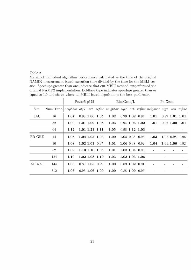
Table 2Matrix of individual algorithm performance calculated as the time of the originalNAMD2 measurement-based execution time divided by the time for the MBLI ver-sion. Speedups greater than one indicate that our MBLI method outperformed theoriginal NAMD2 implementation. Boldface type indicates speedups greater than orequal to 1.0 and shows where an MBLI based algorithm is the best performer.

Power5-p575 BlueGene/L P4-Xeon

Sim. Num. Proc. neighbor alg7 orb refine neighbor alg7 orb refine neighbor alg7 orb refine

JAC 16 1.07 0.98 1.06 1.05 1.02 0.99 1.02 0.94 1.01 0.99 1.01 1.01

32 1.09 1.01 1.09 1.08 1.03 0.94 1.06 1.02 1.01 0.92 1.00 1.01

64 1.12 1.01 1.21 1.11 1.05 0.98 1.12 1.03 - - - -

ER-GRE 14 1.08 1.04 1.05 1.03 1.00 1.05 0.98 0.96 1.03 1.03 0.98 0.96

30 1.08 1.02 1.01 0.97 1.01 1.06 0.98 0.92 1.04 1.04 1.06 0.92

62 1.09 1.10 1.10 1.05 1.01 1.03 1.04 0.98 - - - -

124 1.10 1.02 1.08 1.10 1.03 1.03 1.03 1.06 - - - -

APO-A1 144 1.03 0.80 1.05 0.99 1.00 0.89 1.02 0.91 - - - -

312 1.03 0.93 1.06 1.00 1.00 0.88 1.09 0.96 - - - -

21

Tab

le3:

Com

pre

hen

sive

per

form

ance

dat

afo

rea

chben

chm

ark,pro

cess

orco

unt,

arch

itec

ture

and

algo

rith

m.T

he

low

est

tota

lex

ecuti

onti

me

for

asi

mula

tion

has

bee

nunder

lined

.T

he

bes

tper

form

ing

MB

LIal

gori

thm

ishig

hligh

ted

inbol

dfa

cety

pe

while

the

bes

tper

form

ing

orig

inal

mea

sure

men

t-bas

edal

gori

thm

has

bee

nhig

hligh

ted

init

alic

type.

Tim

esar

ein

seco

nds.

Pow

er5-

p57

5B

lueG

ene/

LP

4-X

eon

Sim

.P

roc.

Tri

alN

oLB

nei

ghbo

ral

g7or

bre

fine

NoL

Bnei

ghbo

ral

g7or

bre

fine

NoL

Bnei

ghbo

ral

g7or

bre

fine

JA

C16

MB

LI

-28

.30

28.4

128

.30

26.8

5-

105.

5810

1.93

107.

27100.3

0-

61.2

260

.02

70.7

756.2

9

Orig

30.2

230

.28

27.9

630

.04

28.2

310

7.16

107.

2910

0.70

109.

1699

.56

58.2

162

.02

59.3

471

.18

56.7

9

32M

BLI

-16

.60

16.6

617

.53

15.7

0-

58.8

959

.13

62.0

254.8

2-

39.6

843

.72

62.1

338.3

5

Orig

18.1

818

.13

16.7

619

.03

17.0

160

.82

60.8

255

.54

65.6

056

.16

41.4

440

.07

40.4

362

.12

38.5

5

64M

BLI

-11

.22

11.0

211

.36

10.2

4-

35.7

133

.37

39.3

131.8

3-

--

--

Orig

12.5

212

.60

11.1

413

.79

11.3

437

.52

37.5

532

.78

44.1

132

.74

--

--

-

ER

GR

E14

MB

LI

-87

.58

77.6

068.1

368

.88

-34

6.24

281.

54266.5

126

9.55

-16

2.18

140.

3713

2.34

130.7

7

Orig

94.1

994

.23

80.6

071

.33

70.9

634

6.49

346.

1529

6.43

260.

6525

8.97

168.

7016

7.11

144.

4612

9.59

125.

74

30M

BLI

-53

.29

41.6

238.0

039

.30

-20

1.27

144.

1913

9.80

147.6

-10

2.57

79.6

678

.03

77.5

3

Orig

57.6

457

.73

42.5

338

.55

38.1

520

3.21

203.

1015

2.34

136.

4613

5.73

99.0

410

6.87

82.5

682

.68

71.2

4

62M

BLI

-31

.33

22.3

521

.78

21.6

0-

109.

3679

.12

74.7

373.8

3-

--

--

Orig

34.1

434

.16

24.6

323

.85

22.6

311

0.86

110.

6581

.56

77.9

372

.70

--

--

-

124

MB

LI

-18

.17

15.9

514

.89

13.8

0-

59.3

445

.54

43.2

640.6

3-

--

--

Orig

20.0

620

.06

16.1

916

.02

15.1

260

.97

60.9

646

.98

44.5

743

.02

--

--

-

AP

O-A

114

4M

BLI

-60

.38

63.1

052

.66

50.2

5-

135.

4012

2.68

126.

38116.1

9-

--

--

Orig

62.0

262

.01

50.5

155

.09

49.5

616

2.60

135.

8810

9.25

129.

5310

5.87

--

--

-

312

MB

LI

-43

.02

40.7

140

.73

37.3

8-

76.0

269

.31

76.0

463.0

2-

--

--

Orig

43.2

044

.16

38.0

342

.99

37.5

282

.76

76.0

160

.92

82.6

760

.61

--

--

-

22

Table 4Table showing the speedups of the best performance for both the original NAMD2implementation and our MBLI implementation. Speedup is calculated as the no loadbalancing time divided by the best performing MBLI or original implementation.Sim. refers to the simulated benchmark, Proc. to the number of processors on whichthe simulation was executed. The definition for δ is given in Section 4.3.2; negativeδ values indicate that MBLI has outperformed the best performing measurementbased algorithm.

Power5-p575 BlueGene/L P4-Xeon

Sim. Proc. Trial Speedup Method δ Speedup Method δ Speedup Method δ

JAC 16 MBLI 1.13 refine 0.039 1.07 refine -0.007 1.03 refine 0.009

Orig 1.08 alg7 1.08 refine 1.02 refine

32 MBLI 1.16 refine 0.063 1.11 refine 0.013 1.08 refine 0.005

Orig 1.08 alg7 1.09 alg7 1.07 refine

64 MBLI 1.22 refine 0.081 1.18 refine 0.028 - -

Orig 1.12 alg7 1.15 refine - -

ER-GRE 14 MBLI 1.38 orb 0.040 1.30 orb -0.029 1.29 refine -0.040

Orig 1.33 refine 1.34 refine 1.34 refine

30 MBLI 1.52 orb 0.004 1.45 orb -0.030 1.28 refine -0.088

Orig 1.51 refine 1.50 refine 1.39 refine

62 MBLI 1.58 refine 0.046 1.50 refine -0.016 - -

Orig 1.51 refine 1.52 refine - -

124 MBLI 1.45 refine 0.088 1.50 refine 0.056 - -

Orig 1.33 refine 1.42 refine - -

APO-A1 144 MBLI 1.23 refine -0.014 1.40 refine -0.097 - -

Orig 1.25 refine 1.54 refine - -

312 MBLI 1.16 refine 0.004 1.31 refine -0.040 - -

Orig 1.15 refine 1.37 refine - -

23

Table 5Standard deviations calculated from wall-clock time per time-step for two sim-ulations on the Power5-p575 (Data corresponds to simulation in Figure 3) andBlueGene/L platforms before and after load balancing for MBLI and the originalNAMD2 implementation.

Standard Deviation

Platform ORIG MBLI

Power5-p575 Total Simulation 0.00368 0.00286

After Load Balance 0.00213 0.00193

BlueGene/L Total Simulation 0.01316 0.01004

After Load Balance 0.01008 0.00874

24