Manufacturing Planning over Alternative Facilities: …sdw1/golbasi1.pdfTechnical Report 99T -10, Department of IMSE, Lehigh Universi ty 1 Manufacturing Planning over Alternative Facilities:

Technical Report 99T-10, Department of IMSE, Lehigh University

1

Manufacturing Planning over Alternative Facilities:

Modeling, Analysis and Algorithms

S. David Wu and Hakan Golbasi

Manufacturing Logistics Institute, Department of IMSE, Lehigh University,

Bethlehem, Pennsylvania 18015

Abstract

We propose a planning model for multiple products manufactured across multiple

manufacturing facilities sharing similar production capabilities. The need for cross-

facility capacity management is most evident in high-tech industries that have capital-

intensive equipment and short technology life cycle. Our model is based on an emerging

practice in these industries where product managers from business units dictate

manufacturing planning in facilities that are equipped to produce their products. We

propose a multicommodity flows network model where each commodity represents a

product and the network structure represents linked manufacturing facilities capable of

producing the products. We analyze in depth the product-level (single-commodity, multi-

facility) subproblem. We prove that even the uncapacitated, general-cost version of this

subproblem is NP-complete. We develop a shortest-path algorithm for this problem and

show that it achieves optimality under special cost structures. We analyze and pinpoint

specific cases where the algorithm fails to produce optimal solutions. To solve the

overall (multicommodity) planning problem we develop a Lagrangian decomposition

scheme, which separates the planning decisions into a number of single-product, multi-

facility subproblems and a resource subproblem. Through extensive computational

testing, we demonstrate that in the context of product-based decomposition the shortest

path algorithm is an effective heuristic for the MIP subproblem, yielding high quality

solutions with only a fraction (roughly 2%) of the computer time.

1. Introduction

This research is motivated by production problems in the electronics, semiconductor and

telecommunication industries. These industries struggle with their production planning problems

in an increasingly complex and rapid changing supply chain environment. Specifically, to better

utilize their capital-intensive equipment they are pressured to produce a wide variety of products


2

in each of their production facilities. However, since these products may each belong to a

different supply channel operating under different delivery and outsourcing contracts and

demand characteristics, production planning decisions are often relegated to product managers

who are most familiar with their specific customer and supplier issues. On the other hand,

production managers must consider resource consolidation and capacity management issues in a

consistent fashion across manufacturing facilities. These competing viewpoints complicate

supply chain planning significantly.

Coordinating production under complex supply structure is not a new problem.

However, two recent trends in these industries exacerbate the intensity of the problem. First, the

trend toward increased market responsiveness intensifies the inter-dependency within the supply

chain. In the past, excess inventory was generally used to reduce the impact of variation across

different facilities. Today, most manufacturers are moving away from carrying substantial

inventories. Second, the rate of technological innovation significantly shortens the life span of

manufacturing equipment, which in term increases the cost of manufacturing capacity. This

combined with increased product variety and decreased product volumes prompt manufactures to

cross-load their manufacturing facilities.

In this paper, we focus on cross-facility operational planning faced by high-tech

manufacturing companies in a supply chain environment. Our research is motivated by

experiences in production management system at a major semiconductor manufacturer for their

world-wide supply base, and by the quantitative supply chain literature. Quantitative analysis of

supply chain management has been focusing on channel design in general and stocking policies

in specific using extensions of inventory, game-theoretic, and strategic models (Tayur et al.,

1999). Cohen and Lee (1988)(1989), Sterman (1989) and Davis (1993) are among the pioneers

who made significant early contributions. Various development of these models remain an area

of active research (c.f., Tayur et al., 1999, Lee, et al. 1995, Hahm and Yano 1995a,b and

Arntzen, et al, 1995). In addition to supply chain design, coordinating various aspects of supply

chain operations has been an area of active research as well. This line of work is exemplified by

Vidal and Goetschalckx (1997), Hahm and Yano (1995a,b), and Ertogral and Wu (1999). A

related, but distinctively different, line of research focuses on the extension of production

models in the context of MRP systems (c.f. Billington, et al., 1983, Carlson and Yano, 1983,

Gupta and Brennan 1995). The focus here is manufacturing planning in the context of multi-

layer and multi-facility production. This line of research is rooted from multi-level, multi-

period, capacitated lot-sizing models. A number of surveys (c.f., Bahl et al. 1987, Goyal and

Gunasekaran, 1990; Baker 1993; Kimms 1997) provide an excellent overview for research in this


3

area. While our proposed model can be linked directly to the multi-level lot sizing literature, it

has two distinctive features that are not previously addressed: first is the explicit consideration of

facility selection decisions. Most existing work assumes either a single facility, or multiple tiers

of facilities as defined by the product structure, but the facility selection decisions are given a

priori. Second, we study a single-item subproblem (with facility selection decisions) that has

been overlooked in the literature. Unlike it’s single-facility counterpart, this subproblem is NP-

complete even in the uncapacitated case. Despite of this, we show analytically and empirically

that a shortest path algorithm could be extremely effective.

2. A Multi-Facility Production Model

We now consider a multi-facility production model where a set of end-items is to be

produced in multiple facilities over multiple periods. Each end-item has a bill of material

described by a product structure. In addition, there is a supply structure where a set of alternative

facilities could be setup to produce each item described in the product structure. Figure 1

illustrates the product and the supply structure. The product structure in Figure 1 can be

represented by a “gozinto” structure common in the lot-sizing literature. The gozinto structure is

specified in an n×n matrix [aik] where aik is the number of item i that is (directly) needed to

produce one unit of item k. In addition to the gozinto structure we define a supply structure

matrix [rij] where rij =1 if facility j could be used to produce item i, and rij = 0 otherwise.

Figure 1. A Supply Network with Three End-Items (1,2 and 3), Six Facilities (I to VI) and a

Maximum of Three Alternative Facilities for an Item

4 1

2 8 5

3

11

9 6

77

10

VI I

II

III

IV

V


4

A Multicommodity Flows Model

The above multi-facility production problem is complex in that the facility selection

decisions are combined with multi-stage, multi-item, multi-period production decisions. To

approach this problem we take the viewpoint of a subset of manufacturing facilities in the supply

network. Each manufacturing facility can produce a variety of products (items) (i=1,2,...,n) over

multiple periods (t=1,2,..,T), while each item i can be produced in a specified set of alternative

facilities (j=1,2,.., Ji ). Each facility can be setup to perform a certain production processes with

a setup cost. Now consider a multicommodity network G(N,A) where each item i corresponds to

a commodity in the network. Let Dt i denote internal demands for item i in period t as defined by

the end-item demand and the product structure. Suppose Dt i can be generated a priori using

standard MRP explosion, we can then define a multicommodity flows network corresponding to

the supply network as shown in Figure 2. This multicommodity flows network has three main

parts: a set of source nodes representing demand dispatching points, a set of sink nodes

representing demand fulfillment points, and a set of production subnets in between each

represents multi-period production to be carried out by a facility. Each commodity (product) i

has a source node si , and T sink nodes d it, one for each period t.

We first describe the overall network structure. The input flow for source node si is the

total demand over T periods for item i (3t4

=1 Dti ), and the outflow on sink note di

t as the

demands for item i in period t,(Dti). The presence of an arc going from source nodes si to facility

subnet j signifies the fact that facility j can be setup to produce item i. These arcs are specified by

the supply structure matrix, i.e., there is an arc (i,j) corresponding to each non-zero entry of

matrix [rij]. The subnets between the set of source and sink nodes represent production facilities

shared by the products. The arcs going from facility subnets j=1,2,.., Ji, period t, to sink node d it

represents that item i’s demand in period t is to be fulfilled by the production and/or inventory

from all (or some) of its Ji alternative facilities. Note that the production subnet can be further

“customized” according the structure of each manufacturing facility. For example, the structure

in Figure 2 shows the familiar single-stage multi-period lot-sizing model. This can be extended

to a multi-stage model (c.f., Afentakis 1984) also shown in the figure, or other multi-period

models. To streamline the analysis, we assume single-stage facility subnets throughout the paper.

We now characterize arc labels in the multicommodity network. Each arc in the network

is characterized by (f i ,c

i, u): arc flow f i, per unit cost ci and arc capacity u. The interpretation of

these values varies according to the types of arcs. The arcs going from source nodes si to the


5

facility subnets j’s are facility selection arcs As ⊂ A, characterized by (xij, c

ij, uij): x

ij represents

the total production to be performed on facility j over t=1,..,T, cij represents the arc cost that

quantifies the differences among facilities (e.g., quality history, reputation), and capacity uij

represents the maximum amount of item i that can be produced in facility j. When the dynamic

lot-sizing model is used in the production subnet, two types of arcs are used: arcs going from left

to right are production arcs Ap⊂ A, characterized by (xijt, c

ijt, capjt): production quantity xi

jt, unit

production cost cijt ,and production capacity capjt = u. Arcs going from top down are inventory

arcs AI⊂ A characterized by (Iijt ,hi

jt , invjt ): inventory carried from period t to t+1, I ijt, unit

inventory holding cost cijt, and inventory limit invjt = u. Finally, an arc going from facility j

period t to sink node d it belongs to the demand arcs Ad⊂A, characterized by (bi

jt, rijt, capjt): b

ijt

represents facility j’s contribution to demand Dit,, ri

jt represents the transportation cost from

facility j to the demand point i ,and capjt is the transportation capacity in period t.

3 t4=1 Dt

1

3 t4

=1 Dt2

3 t4=1 Dt

3

D11

D21

D31

D41

A multi-stage extension of theproduction resource subnet(index l represents stages)

Facilitysubnet j

x ijt

Iijt

(Dti )

x ijt l

Iijtl

*The network represents a facility with 3 products, 3 production lines and 4 periods

si dti

x ijt

b ijt

Figure 2. A Multicommodity Flows Network for a Three-Item, Three-Facility, Four-Period

Model

Given the above specification, we can define the general multicommondity constrains (1.1) and

(1.2) as follows:

General arc capacity constraints for all arcs


6

dI

n

ipjt

ijt

ijt

sijij

AAAtjuf

Ajiux

∪∪∈∀≤

∈∀≤

∑=1

),(

),(

β (1.1)

where β is the capacity consumption rate. Denote a the node-arc incidence matrix for the multicommodity flows network G(N,A) and ei the net balance flows for commodity i. The mass balance constraints are as follows:

Mass balance constraints for each commodity Nief ii ∈∀= a (1.2)

In addition to the general multicommodity flows constraints as specified by the network structure

G(N,A), we define additional constraints for each facility submodel. Consider the multi-period

lot-sizing model we use for all facility subnets. While the inventory balance constraints are part

of the mass balance constraints (1.2), we need to define additional constraints due to setup. Let

αijt denote the rate of capacity consumption for setup activities, δi

jt a binary variable indicating

the existence of a setup for item i at facility j at period t. The production specific constraints are

as follows:

Production capacity constraints for production and setup

∑∑= =

∈∀≤+n

i

J

jpjt

ijt

ijt

ijt

ijt

i

Atjcapx1 1

),( )( δαβ (2.1)

Setup constraints

pijt

ijt AtjNiMqx ∈∈∀≤ ),(, (2.2)

Up to this point we ignore the fact that the items entering the production facilities (as

represented by the multicommodity flows network G(N,A)) has an underlying product structure

[aik]. To model the supply structure as well as the product structure across multiple tiers of a

supply chain, we will need to include additional constraints which specify the relationship among

demands of items over time Dit, i=1,…,n, t=1,…,T. First of all, the demand for end-items, N0 ⊆

N, must be satisfy. Although this is already implied in the mass balance constraints (1.2), we

will restate it for clarity.

Demand for end item must be satisfied

01

, NitDb it

m

j

ijt ∈∀=∑

=

(3.1)

The end-item demand triggers the internal demands in the supply chain as defined by the product structure. Denote Lk the lead-time for item k, we can define the following relationship:


7

Demand internal the supply chain must be satisfied in each period

011

, NNitDabn

k

kLtik

m

j

ijt k

−∈∀= ∑∑=

+=

(3.2)

Denote cijt and hi

jt, respectively, the production and the inventory holding costs for item i at

facility j during period t, and Kij, the set-up cost for item i at facility j, and ri

jt the unit

transportation cost from facility j to the demand point. We state an objective function with these

cost components defined for the production subnet. A cost component unique to each product i,

say Si(f i,ci,u), could be added to the objective to reflect special requirements imposed by the

supply channel of i. Since this does not affect our analytic results significantly, we will not

consider this cost terms here. Thus, a multicommodity flows formulation of the multi-facility

production problem (P) is as follows:

Problem (P):

∑∑∑= = =

+++=T

t

n

i

J

j

ijt

ijt

ijt

ijt

ijt

ij

ijt

ijt

i

brIhKxczMinimize1 1 1

)( δ

s.t. <General Multicommodity Flows Constraints (1.1)-(1.2)> <Production Specific constraints (2.1)-(2.2)> <Supply-Chain Specific constrains (3.1)-(3.2)> (4) nonnegativity constraints

(5) binary constraints

It is useful to note that in this multicommodity flows model, only the capacity constraints

(1.1) and (2.1) are bundling constraints. All the other constraints can be decomposed by

commodity (product). (P) is a multi-period, multi-item, multi-facility production planning model.

3. Model Analysis

Note that since the mass balance constraints (1.2) imply NiDb it

m

j

ijt ∈∀=∑

=

,1

, constraints

(3.2) in effect specify the relationship between the demands of item i and the items (k’s) which

use i as a component, i.e.,

01

, , NNitDaDn

k

kLtik

it k

−∈∀= ∑=

+ (3.3)

0,,,, ≥ijt

ijt

ijt

ijt

i bIxf δ

)1 ,0(∈ijtδ


8

Consider a set of facilities in a manufacturing supply chain as depicted in Figures 2.

Suppose the end-item demand is stationary, the relationship in (3.3) suggest that it is possible to

generate Dit a priori using a BOM explosion mechanism frequently used in MRP systems, i.e.,

we may treat Di as parameters generated and fixed a priori for the multicommodity flows model

such that (3.2) is always satisfied. This simplifies the facility selection decisions considerably

since we do not need to make the multi-tier production planning decisions all at the same time.

This corresponds to the practice in most industries where the demand information across

different tiers of the supply chain are announced ahead of time according to built-in leadtimes

(rather than pulled instantaneously).

To explore special subproblem structures that will later help the solution of model (P),

we consider two submodels in the following sections.

3.1 Uncapacitated Single-Item, Multi-Facility Model without Transportation Costs

As stated above, model (P) can be decomposed by commodity after relaxing the bundling

capacity constraints (1.1) and (2.1). We first consider a capacity-relaxed single-item, multiple-

facility subproblem (without transportation costs) for commodity i as follows:

(Pi) ∑∑= =

++T

t

J

jjtjtjjjtjt

i

IhKxcMinimize1 1

)( δ

s.t. <mass balance constraints for commodity i (1.2)> <setup constraint for commodity i (2.2)>

<constraints (4)(5) for commodity i>

Subproblem (Pi) represents a subset of the decision problem for the product manager of i who

must decide where to produce her product among a certified1 set of manufacturing facilities Ji.

Note that we dropped the cost component Si(f i,ci,u) from the objective, hence the facility

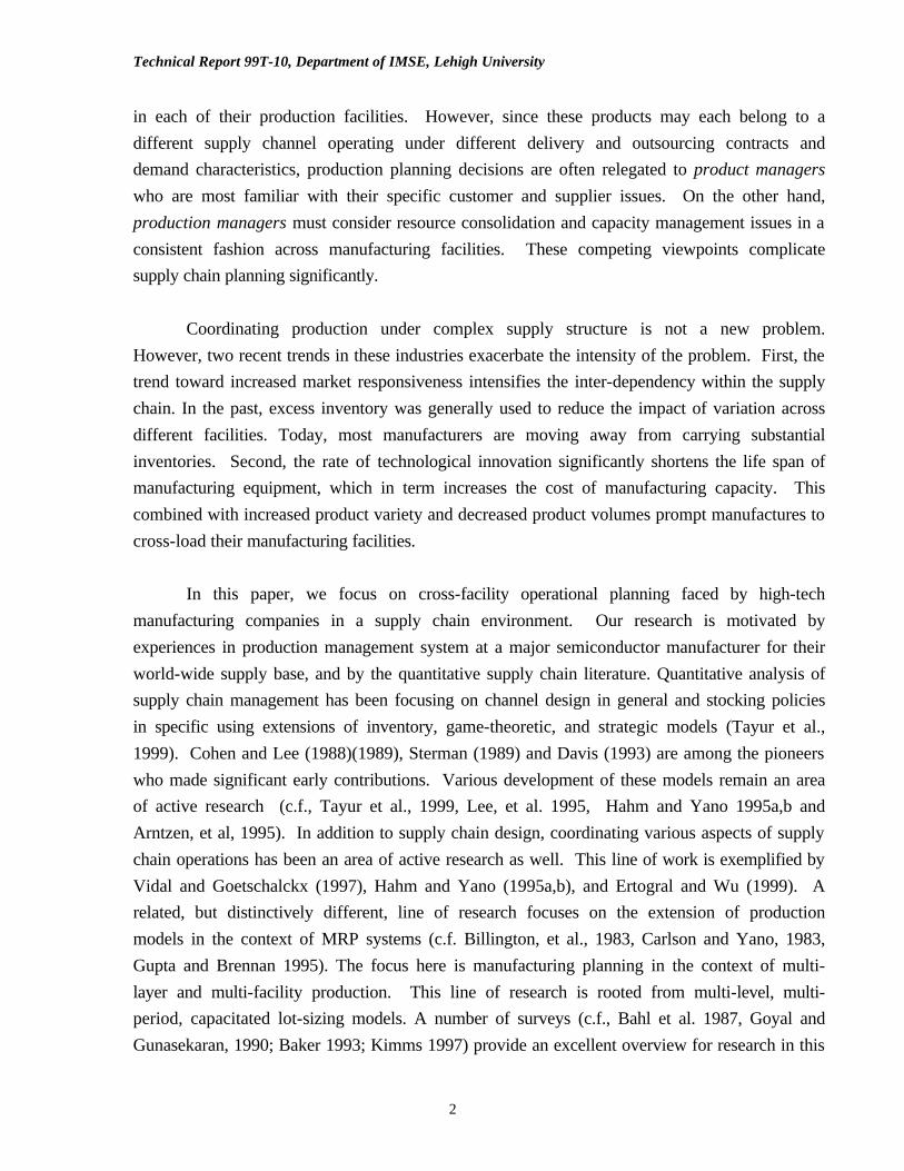
selection and the transportation costs are assumed to be zero. Figure 3 depicts a subnetwork

defined by commodity 1 (for problem (P1)) corresponding to the example in Figure 2.

While the above facility-selection/lot-sizing problem has not been well studied, the

single-facility, single-item, uncapacitated lot-sizing problem has been studied intensively in the

literature. Despite of the binary variables it is well known that this problem can be solved in

polynomial time using Wagner-Within type algorithms. In recent years, more efficient

implementation of Wagner-Within algorithms has been developed (c.f., Federgruen and Tzur

(1991) and Wagelmans et al. (1992)), which has order O(n log n) or better. Embedding these

1 The notion of facility certification is important in Semiconductor Manufacturing where a product can only produce in a facility that has been pre-certified for quality and yield.


9

polynomial-time solvable problem as submodels, the multi-item, capacitated lot-sizing problems

are frequently solvable in a reasonable amount of time for realistic size problems (c.f.

Tempelmeir and Derstroff, 1996). Since a primary new consideration in our model (P) is the

selection of alternative facilities, it is important to know the structure and the complexity of

subproblem (Pi). This analysis is important to the solution of (P) since (1) (Pi) has the form of a

mixed integer program, and (2) there is no straightforward (efficient) decomposition from the

multi-facility case to single-facility. In the following, we first show that (Pi) is NP-complete

when the holding cost hjt is general and not restricted in sign. We then show that an efficient

algorithm exists under a special set of conditions. Later in Section 4 we show computationally

that under general cost conditions this algorithm is an effective heuristic, solving most instances

of (Pi) optimally.

3 t4

=1 Dt1

D11

D21

D31

D41

Facilitysubnet j

b ijt

Figure 3. Subnetwork Corresponding to Commodity 1, with 2 alternative facilities, 4 periods

Theorem 1. (Non-splitting property): There exists an optimal solution to the uncapacitated,

single-item, multiple facility problem (Pi) such that item i's demand in period t is satisfied by the

production or the inventory of exactly one of the Ji facilities, i.e., exactly one bijt among j=1,..,Ji

is non-zero (=Dit) for each period t.

Proof: see Appendix.


10

As we shall see in the following exploration, the insight provided by the non-splitting property

plays an important role in the development of solution algorithms for the uncapacitated

subproblem (Pi) as well as the overall problem (P). Nonetheless, despite of its promising

outlook, subproblem (Pi) can be only solved efficiently under more restrictive conditions due to

the existence of several pathological cases. In the following, we first show that under

generalized cost condition subproblem (Pi) is NP-Complete.

Theorem 2. The uncapacitated, single-item, multiple-facility problem is NP-Complete when the

inventory holding cost hjt is a generalized cost coefficient not restricted in sign.

Proof: see Appendix.

Upon examining the proof it should be clear why NP-Completeness can be only constructed for

the case where arc cost is not restricted in sign. In the following, we show that the NP-complete

status remains when the demands or the setup costs are constant.

Corollary 1. The problem stated in Theorem 1 remains NP-Complete when the period demands

Dt are constant over periods t=1,..,T.

Corollary 2. The problem stated in Theorem 1 remains NP-Complete when the setup costs Kj

are constant across facilities j=1,…,m.

In the following, we go on to show that despite of the NP-complete status of problem (Pi) and its

variations, under mild assumptions a shortest path algorithm solves problem (Pi).

The uncapacitated, single-item, multiple-facility problem (Pi) can be solved in

polynomial time using a shortest path algorithm if and only if the following conditions hold:

(i) No simultaneous production of item i over more than one facility can take place in a

given period. In other words, x ijt xikt=0, ∀ i,j,k≠j,t.

(ii) No production of item i will be scheduled at all if there is inventory carried over from a

previous period in one of the facilities. In other words, x ijt I ikt-1=0, ∀ i,j,k,t.

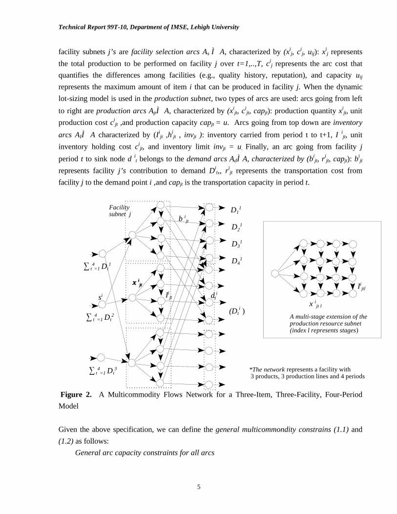
Proof: We will state the proof using a familiar graphical representation as in Figure 4. The first

row of nodes denotes facility 1 and the ith row denote facility Ji. There are T+1 time

epochs:0,1,2,3, and a period is the interval between epochs, i.e., between epochs 0 and 1 is

period t=1, and between 1 and 2 is period t=2, etc. A horizontal arc denotes the production that

satisfies all the periods' demand within the time epochs. The arc cost includes production,

inventory and setup costs. A vertical arc denotes a switch from one facility to another and the


11

cost associated to these arcs are 0. There is an artificial source and sink, arcs adjacent to these

nodes have 0 cost. In a general graph for each time epoch there are arcs for all the facility

periods. So production of an item may switch from one facility to any other in different periods.

From condition (ii), there will be production scheduled for item i only if there is no inventory

carried over from a previous period in one of the facilities. In other words, in an optimal solution

exactly one arc will be chosen to enter a given node in the network. On the other hand, condition

(i) states that there can be no simultaneous production of items i in more than one facility in any

given period. In other words, in an optimal solution exactly one arc will be chosen to leave a

node in the network. This means that an optimal production schedule corresponds to a source-to-

sink path in the network, and it corresponds to a shortest cost path. ð

Figure 4. The Multi-Facility Production Problem as a Shortest Path Problem

Unfortunately, there are cases where conditions (i) and (ii) in Proposition 1 do not hold in

the optimal solution. This is caused by pathological cases such as the follows: under completely

general production and inventory holding costs, it could be optimal to produce x ijt in a facility j

in period t, holding this amount in the inventory for a future period t+l (l>1) without using it in

periods t+1,…, t+l−1. Since more than one facility may produce, the demands in periods t+1,…,

t+l−1 could be satisfied by a number of facilities other than j. This creates the possibility of

“multiple-path” production (see Figure 5). For instance, in Figure 5-(b), a production is started in

period 1 at both facility 1 and 2, while the former is used to satisfy demands in periods 2 and 3,

the latter is produced for period 1. This is possible when the production cost for facility 1 in

period 1 is higher than that of the facility 2, but the combination of production and holding costs

for periods 2 and 3 is lower in facility 1 than that of facility 2. Note that this particular case

violates condition (i) and no shortest path algorithm will identify this as a solution. Similarly, in

Periods

Facility 1

Facility Ji

••••

••••

Periods

• • • •

• • • •


12

Figure 5-(a),(c),(d), condition (ii) is violated since a production takes place in one facility despite

of the fact that the other facility holds inventory.

Proposition 2. When it is optimal to start a production at facility j in period t for a future period

t+l ( l>0) while the demands in periods t,…,t+l-1, are satisfied by facilities other than j (none of

j’s inventory is consumed during t,…,t+l-1), then subproblem (Pi) can be no longer solved by a

shortest path algorithm.

Proof. It is sufficient to make an observation that under the above situation either condition (i)

or (ii) in Proposition 1 will be violated. It is known from the Leontief structure that bi jt for a

facility j can be either Dit or 0. Suppose the demand for period t is satisfied by facility k but not

facility j, i.e., for facilities j and k, bijt=0 and bi

kt=Dit, respectively. Since xi

jt+ Iijt-1 − Ii

jt=bijt, ∀ j,t

it is possible to have

(Case 1) (xijt= Ii

jt =Dit+l and Ii

jt-1=0) and (xikt= Di

t and Iikt=Ii

kt-1) (violation of condition (i))

(Case 2) (xijt=0 and Ii

jt=Iijt-1= Di

t+l ) and (xikt= Di

t and Iikt=Ii

kt-1) (violation of condition (ii))

Recall that conditions (i) and (ii) in Proposition 1 are as follows:

(i) xijt x

ikt=0, ∀ i,j,k≠j,t,

Facility 1

Facility 2

Facility 1

Facility 2

Facility 1

Facility 2

Facility 1

Facility 2

Denotes that demand is satisfied by that facility

Denotes a production takes place in the period where the arrow emanates from, which covers the demands up to the period where the arrow terminates

Figure 5. Four examples cases where the Shortest Path Algorithm may fail

t1 t2 t3 t1 t2 t3

(a)

(c)

(b)

(d)


13

(ii) x ijt I ikt-1=0, ∀ i,j,k,t.

In Case 1 above, it is clear that condition (i) is violated while in Case 2, condition (ii) is violated

�

The fact that the shortest path algorithm is not always optimal for subproblem (Pi) should

not come as a surprise as Theorem 2 shows that the generalized cost version is NP-

Complete. Nevertheless, the shortest path algorithm is a valid heuristic for subproblem

(Pi). In the computational experiments, we will show that the shortest path algorithm is

an effective heuristic, yields optimal or near-optimal solutions in most test cases.

3.2 Uncapacitated Single-Item, Multi-Facility Model with Transportation Costs

Recall that in the multicommodity flows network (Figure 2) and the single-item

subnetwork (Figure 3) a demand arc Ad⊂A goes from facility j period t to demand point d it is

characterized by (bijt, ri

jt, capjt) where bijt represents facility j’s contribution to demand Di

t,, rijt

represents the transportation cost from facility j to the demand point i, and capjt is the

transportation capacity in period t. In Section 3.1 we assume the transportation cost rijt=0 and

capjt=4. We will now consider the single-item subproblem where the transportation cost is

positive but we will not consider transportation capacity. The subproblem can be stated as

follows

(P’i) ∑∑

= =

+++T

t

J

jjtjtjtjtjjjtjt

i

brIhKxcMinimize1 1

)( δ

s.t. <mass balance constraints for commodity i (1.2)> <setup constraint for commodity i (2.2)>

<constraints (4)(5) for commodity i>

Theorem 3. The uncapacitated, single-item, multiple-facility problem with non-negative

transportation cost rjt is NP-Complete.

Proof. See Appendix.

Algorithm Complexity

We now explore possible algorithms for problem (P’i) and their complexity as related to the

number of facilities and number of periods. A first observation is by viewing the single-item,

multi-facility problem depicted in Figure 3 as a Directed Steiner Tree Problem (Leibling, 1999):

the subnetwork represents the problem graph, while the source, the root of each production

subnet, and the demand nodes (on the right) are “compulsory” nodes, the remaining are


14

“optional” or Steiner points. The Directed Steiner Tree Problem is to find an arborescence of

minimal total length that spans all compulsory nodes using one or more Steiner points. Suppose

arc lengths can be determined a priori using production, inventory, and transportation costs, an

optimal Steiner solution corresponds to an optimal solution to (P’i). It is known that a dynamic

programming algorithm (Dreyfus and Wagner, 1972) solves the Steiner Problem in

]2)(3)[( 2 ss Nsc

Nsc NNNNO ⋅+++ where Ns is the number of Steiner points (i.e., number of

facilities × number of periods) and Nc is the number of compulsory points (i.e., number of

periods). While this observation suggests that a dynamic programming algorithm constructed in

this fashion is exponential in the number of facilities and period, using the well-known Wagner-

Within results, we could improve the complexity significantly. This is stated as follows.

Theorem 4. There exists an algorithm for the uncapacitated, single-item, multiple-facility

problem with non-negative transportation cost (Problem (P’i)) that is polynomial in the number

facilities and exponential in the number of periods.

Proof. Consider a simple algorithm as follows for problem (P’i):

(1) Assign demands D1,…,DT to facilities j=1,…,m (this takes O(mT))

(2) Given the assignment, solve for each facility j=1,…,m an uncapacitated, single-item, single-

facility lot-sizing problem using the Wagner-Within Algorithm (this takes m⋅O(T logT))

The algorithm has complexity O(mT+1⋅T log T), which is polynomial in the number of facilities

but exponential in the number of periods. ÿ

Special Cost Structure

Despite of the negative results, the shortest path algorithm remains a viable option under certain

cost structures. Specifically, when transportation and production costs are fixed, when there is

no incentive to hold inventory for more than four periods without starting a new setup, and when

holding inventory in a facility j for two periods always costs more than holding inventory

elsewhere for one period (i.e., when holding costs are not dramatically different), all pathological

cases stated in Proposition 2 and Figure 5 disappear.

Proposition 3. The uncapacitated, single-item, multiple-facility problem with non-negative

transportation cost (P’i) can be solved in polynomial time using a shortest path algorithm if the

following conditions hold:

(i) The transportation and the production costs are fixed across facilities and periods

(ii) There is no setup that would last more than four periods, i.e., jKDh j

t

tj ∀≥∑

+

=

,3

ττ

τ

(iii) Inventory holding costs of any two facilities j and k satisfies the relationship


15

tkjhhh tktjjt ,,1,1, ∀≥+ ++ .

It should be intuitive when conditions (i)-(iii) above hold in the data set, the condition in

Proposition 2 is eliminated, while conditions (i) and (ii) in Proposition 1 will be satisfied,

i.e., the shortest path algorithm will produce optimal solution. These conditions can be

thus used as a test to be performed on the data set before calculation starts. It is quite

likely that even when the above conditions are violated, the shortest path algorithm

remains an effective heuristics. To put this point under solid empirical testing, we

conducted two sets of computational experiments: the first experiment simply compares

the optimal solutions for (Pi) obtained by a MIP (Mixed Integer Programming) solver vs.

solution provided by a shortest path algorithm. The results are summarized in Section

3.4. The second set of experiments is more complicated, here we test the quality of the

single-item shortest path algorithm as a subproblem heuristic for the multi-item problem

(P). This will be detailed in Section 4.

3.4 Performance of the Shortest Path Algorithm

To instantiate the insights gained from the analytic results, we conduct intensive

empirical testing by varying setup, holding, production, and transportation costs, the

number of facilities and periods combinations, and levels of demand lumpiness. This

results in 17,500 instances. We first generate a nominal case as follows:

Setup cost , Kj~Uniform[1500,3500]

Production cost, cjt~Uniform[5,15]

Transportation cost, rjt~Uniform [5,15]

Holding cost, hjt~Uniform[5,15]

Number of facilities: 4

Number of periods: 6

Demand Dt~Uniform[5,15]

No demand lumpiness

Demand lumpiness is used to generate clustered demand patterns more closely resemble

practical situations. While generating random demand for Dt period t, we first generate a

random number between 0 and 1, if it is less than the current lumpiness threshold ζ, then

Dt is set to 0, otherwise, Dt set to the generated demand. We adjust the demand levels

such that the expected demand remains the same as the base case.

By varying one or more factors from the nominal case, we generate three groups of test

problems as follows:


16

(Group One): Fixed setup cost across all periods, i.e., setup cost is generated once and

fixed for all periods (by varying the following cost factors, we generate 65 sub-groups

where 100 replications are generated for each subgroup)

a1-a10: varying the setup cost levels from Uniform [0,500] to Uniform [5000,10000]

a11-a20: varying the holding cost levels from Uniform [1,5] to Uniform[100,200]

a21-a30: varying the production cost levels from Uniform[1,5] to Uniform [100,200]

a31-a40: varying the transportation cost levels from Uniform[1,5] to Uniform[100,200]

a41-a60: varying the number of facilities (Ji)/number of periods (T) combinations, or

|Ji|×|T| where |Ji|=2,3,4,5,6 and |T|=6,8,10,12

a61-a65: varying the demand lumpiness threshold ζ= 0, 0.2, 0.3, 0.4, 0.5

(Group Two): Variable setup cost across periods, i.e., setup costs are randomly generated

for each period t. Again, 65 sub-groups are generated as above with 100 replications

each.

(Group Three): Fixed production and transportation costs, i.e., the production and

transportation costs are fixed to their expected value (10). This eliminates subgroups

a21-a40 above, resulting in 45 subgroups with 100 replications each.

A summary of the test results is given in Figure 6. As shown in the Figure, except

for subgroups a37-a40, the shortest path algorithm produces nearly identical solutions as

the MIP (i.e., less then 3 occurrences per 100 instances, with a maximum solution

deviation less than 0.2%). When more significant deviations are observed in subgroups

a37-a40 (cases where the transportation costs are high at Uniform [40,80], …, Uniform

[100,200], respectively), although the number of occurrences are much more pronounces

(up to 49 per 100 instances), the maximum amount of deviation is still under 0.5% in all

cases. The number of occurances are more pronounced when the setup costs are variable

across periods (Group Two). Now consider the Group Three results: there is no deviation

between shortest path and MIP solutions in any of the 4,500 cases tested. Consider this

result along with Proposition 3. It is interesting to note that when the production and

transportation costs are fixed (condition (i) in the proposition), even when conditions (ii)

and (iii) do not hold, the shortest path algorithm produces optimal solutions. These results

confirm our insight from Proposition 2 that pathological cases exist where the shortest

path algorithm produces sub-optimal solutions; upon examining these cases, we found

that they are indeed caused by circumstances depicted in Figure 5. On the other hand, the

empirical results show that the shortest path algorithm is a very effective heuristic for the

single-item, multi-facility subproblem. In the following section, we consider this single-

item subproblem in the context of the Multi-Item problem.


17

Group One: Fixed Setup

0

10

20

30

40

50

60

a1 a5 a9 a13 a17 a21 a25 a29 a33 a37 a41 a45 a49 a53 a57 a61 a65

Sub-Groups

Nu

mb

er o

f O

ccu

ran

ces

ou

t o

f 10

0

00.010.020.030.040.050.060.070.080.090.1

Max

imu

m %

of

Dif

fere

nce

s

Group Two: Variable Setup Costs

0

10

20

30

40

50

60

a1 a5 a9 a13 a17 a21 a25 a29 a33 a37 a41 a45 a49 a53 a57 a61 a65

Sub-Groups

Nu

mb

er o

f O

ccu

ran

ces

ou

t o

f 10

0

00.010.020.030.040.050.060.070.080.090.1

Max

imu

m %

of

Dif

fere

nce

Group Three: Fixed Production and Transportation Costs

In all 4,500 instances in this group, the Shortest Path Algorithm produces the same solution as the Mixed Integer Program, i.e., the number of occurrences and the maximum % of difference are 0 in all cases.

Figure 6. Comparing the Shortest Path and the MIP Solutions


18

4. A Solution Methodology for the Multi-Item, Multi-Facility Problem (P)

We propose a Lagrangean Decomposition scheme for the solution of the multi-item, multi-

facility problem (P) where the single-item problem (Pi) is a subproblem. Lagrangean

Decomposition, as described in Guignard and Kim (1987), has been applied to a variety of NP-

hard problems including multi-item single-facility lot-sizing problems (Thizy, 1991). A main

advantage of Lagrangean Decomposition over the better known Lagrangean Relaxation is that

the theoretical Lower Bound obtained from Lagrangean Decomposition is at least as tight as that

from Lagrangean Relaxation. We start our exposition by first listing the mass balance constraints

(1.2) explicitly:

(1.2.4) ,

(1.2.3) ),(,

(1.2.2) ,

(1.2.1)

1

1

1

11

TtNiDb

AtjNiIbIx

JjNixf

NifD

it

J

j

ijt

ijt

ijt

ijt

ijt

T

ti

ijt

ij

J

j

ij

T

t

it

i

i

∈∈∀=

∈∈∀+=+

∈∈∀=

∈∀=

∑

∑

∑∑

=

−

=

==

If we assume that the system must return to its initial inventory at the end of the planning

horizon, i.e., I0 = IT , we may simplify the above mass balance constraints. From (1.2.3) and

(1.2.4) we have,

∑∑∑

∑∑∑ ∑

∑ ∑ ∑∑

= ==

=

−

==

−

=−

= = = =−−

∈∀=

=+=+=

=

−+=∀−+=

i

i i

J

j

T

t

ijt

T

t

it

T

t

ijtT

T

t

ijt

T

t

T

t

ijt

ijt

T

J

j

T

t

T

t

J

j

ijt

ijt

ijt

it

ijt

ijt

ijt

it

NixD

IIIIII

II

IIxDtiIIxD

1 11

1

1

11

1

101

0

1 1 1 111

)6.2.1( ,

as (1.2.5) rewritecan weso ,

sincebut

(1.2.5) )( thus,,, )(

Note that (1.2.6) implies constraints (1.2.1) and (1.2.2). This allows us to consider problem (P)

with only two sets of balance constraints (1.2.3) and (1.2.4) since (1.2.1) and (1.2.2) will be

satisfied automatically. Now, consider the objective function of (P):

∑∑∑= = =

+++=T

t

n

i

J

j

ijt

ijt

ijt

ijt

ijt

ij

ijt

ijt

i

brIhKxczMinimize1 1 1

)( δ

Since ijt

ijt

ijt

ijt IIxb −+= −1 (from (1.2.3)), the objective can be re-rewritten as follows:

∑∑∑= = =

+ ++−++=T

t

n

i

J

j

ijt

ij

ijt

ijt

ijt

ijt

ijt

ijt

ijt

i

KIrrhxrczMinimize1 1 1

1 ))()(( δ


19

If we set ijt

ijt

ijt

ijt

ijt

ijt

ijt rrhhandrcc 1

ˆˆ ++−≡+≡ to be the generalized production and holding costs,

the objective becomes:

∑∑∑= = =

++=T

t

n

i

J

j

ijt

ij

ijt

ijt

ijt

ijt

i

KIhxczMinimize1 1 1

)ˆˆ(( δ

The basic idea of our decomposition is to separate the multicommodity flows problem (P) into

two subproblems: the first with the capacity and the mass balance constraints, but not the setup

constraints, the second is a commodity-decomposable subproblem with the mass balance and the

setup constrains. The latter defines separable single-item problems (Pi), which has special

structure as analyzed in Section 3. In this decomposition, the first subproblem is a linear

program and the second is a collection of MIP problems. If we make use of the shortest path

algorithm for each MIP (as a heuristic), all subproblems are easy to solve. To demonstrate this

solution methodology we use a slightly simplified formulation of problem (P) by dropping the

first term in the objective (as above), and assuming that setup does not consume capacity

(dropping (2.1)). We then restate the multi-facility production problem (P) with duplicated

variables as follows:

(P’)

(4.3) ,)(

(4.2) ),(, 0

(4.1) ),(

..

)ˆˆ((

11

1

1

1 1 1

TtNiDIIx

AtjNiIIx

Atjux

ts

KIhxczMinimize

it

J

j

ijt

ijt

ijt

ijt

ijt

ijt

n

ijt

ijt

ijt

T

t

n

i

J

j

ijt

ij

ijt

ijt

ijt

ijt

i

i

∈∈∀=−+

∈∈∀≥−+

∈∀≤

++=

∑

∑

∑∑∑

=−

−

=

= = =

β

δ

(4.9) ,, )1,0(

(4.8) ,, 0,

(4.7) ,, 0,

)6.4(,,

)(4.3 ,)(

)(4.2 ),(,0

(4.5) ,,

(4.4) ,,

11

1

TtJjNi

TtJjNiIIxx

TtJjNiIx

TtJjNiMxx

TtNiDIIIIxx

AtjNiIIIIxx

TtJjNiIII

TtJjNixxx

ijt

ijt

ijt

ijt

ijt

ijt

ijt

it

J

j

ijt

ijt

ijt

ijt

ijt

ijt

ijt

ijt

ijt

ijt

i

∈∈∈∀∈

∈∈∈∀≥

∈∈∈∀≥

∈∈∈∀≤

′∈∈∀=−+

′∈∈∀≥−+

∈∈∈∀=

∈∈∈∀=

∑=

−

−

δ

δ


20

In the above formulation, we make copies of the variable xijt, b

ijt, and Ii

jt as xxijt, bbi

jt, and IIijt.

We then use the copies to split the original constraints into two sets of constraints: {(4.1)-

(4.3),(4.7)} and {(4.2)′,(4.3)′,(4.6),(4.8),(4.9)} plus the linking constrains (4.4)-(4.5). It should be

clear that (P) ≡≡(P’). We then separate (P′′) by relaxing the linking constraints and placing them in

the objective function with Lagrangean multipliers λxijt and λI

ijt. This yields the following

subproblems:

Resource Subproblem:

)7.4(),3.4(),2.4(),1.4(..

)())ˆ()ˆ((Minimize 11 1 1

1

ts

zIhxczT

t

n

i

J

j

ijt

Iijt

ijt

ijt

xijt

ijt

i

λλλ ≡+++= ∑∑∑= = =

n Product Subproblems:

(4.9)(4.8),(4.6),,)(4.3,)(4.2 ..

)())((Minimize1

21 1 1

2

′′

≡+−−= ∑∑ ∑∑== = =

ts

zqKIIxxzn

i

in

i

T

t

J

j

ijt

ij

ijt

Iijt

ijt

xijt

i

λλλ

Note that under the general framework of Lagrangean Decomposition, constraints (4.2) and (4.3)

do not need to be duplicated for both subproblems, i.e., these constraints can be assigned to

either subproblems. However, our computational experience indicates that as long as the added

constraints do not add computational burden to the subproblems, constraint duplication improves

the speed of convergence and yield better lower bounds since the solutions proposed by the

subproblems tend to be similar. A lower bound to problem (P′′) given Largrangean multiplier set

λ is as follows:

∑=

+=′n

i

izvzvPLB1

21 ))(())(()( λλλ

Where v(.) denote the optimal value of the objective. Note that the resource subproblem

is a linear program, and the product subproblem zi2 has similar structure as problem (Pi)

described earlier. From the lower bound solution, an upper bound for problem (P’) can be

generated using the following feasibility restoration routine: given the solution for the resource

subproblem we add setups for the periods where production is nonzero, i.e., we set qijt to 1

whenever xijt>0. We then calculate the objective function using the original cost function. This

results in an upper bound for the original problem. The lower bound can be maximized by


21

searching for the set of Largrangean multipliers λ that maximize the Lagrangean dual. Both dual

ascent and subgradient search methods can be used for this task. In this paper, we use the latter

approach, which is summarized in the following Section 4.2. As we will demonstrate in the

computational section, we can achieve solutions with very small duality gaps using the bounds

and the search algorithm.

4.1. Managerial Insights Related to the Decomposition

Our choice of Lagrangean Decomposition is not purely motivated by computing. The

decomposition of the multi-facility production model into a resource subproblem and multiple

product subproblems has interesting managerial implications. As recognized by several

researchers (c.f., J`rnsten and Leisten, 1994; Burton and Obel, 1984), mathematical

decomposition often leads to insights for general modeling strategies or even new decision

structures. The decomposition suggested earlier allows further analysis concerning modeling

flexibility in the context of multi-facility manufacturing planning. Suppose we consider each

product subproblem as a decision problem for a product manager and the resource subproblem as

a decision problem for a production manager overseeing multiple facilities. Thus, the

decomposition can be viewed as a decision system where product managers, each responsible for

a product, compete for resource capacity available from manufacturing facilities. The production

manager, on the other hand, represents the interests of efficiently allocating resources from

multi-facilities to the products. Clearly the solutions proposed by the production manager (x, I)

do not agree with the collective solution proposed by the product managers (xx, II). A search

based on Lagrangean multipliers essentially penalizes their differences, while adjusting the

penalty vector iteratively. This process stops when the degree of disagreement (the duality gap)

is acceptably low, or when further improvement is unlikely.

The above viewpoint is useful in evaluating the flexibility model (P) represents. First, it

should be clear that each product subproblem (Pi) could be customized to represent the

distinctive needs of each product. So long as its basic network structure is maintained there will

be no additional computational burden. Similarly, as long as the resource subproblem remains a

linear program, it can be customized with various facility submodels each reflecting the distinct

production structure of a facility. However, a different constraint duplication strategy may be

necessary when changes are made to the base model.

4.2. The Subgradient Search Algorithm

In this section, we summary the subgradient search algorithm used to adjust the

Lagrangean multipliers. At each iteration s, we calculate Lagrangean multipliers using the

following equations:


22

)(

)(

,,,1,

,,,1,

sijt

sijt

ssIijt

sIijt

sijt

sijt

ssxijt

sxijt

IIIu

xxxu

−+=

−+=+

+

λλ

λλ (4.10)

where

∑∑∑

∑

= = =

=

−+−

+−

=T

t

n

i

J

j

sijt

sijt

sijt

sijt

n

i

sisss

s

i

IIIxxx

zvzvUB

u

1 1 1

2,,2,,

121

*

))()((

)))(())(((( λλγ

(4.11)

γs: a scalar set to 1 and reduced by half if the lower bound fails to improve after a

fixed number of iterations

UB*s: the best upper bound obtained up to iteration s

In our testing, we terminate the algorithm after a prespecified number of iterations. The best

upper bound obtained at the end of the iterations provides the heuristic solution to the problem.

We summarize the algorithmic steps as follows:

Step 1: Initialize s,λ,u, γ and UB*.

Step 2: Solve the resource and the product subproblems. Compute the lower bound

∑=

+n

i

sis zvzv1

21 ))(())((( λλ for current iteration, s.

Step 3: Compute an upper bound UBs from the optimal solution of the current resource

subproblem Min z1(λs). If *1−< ss UBUB , set ss UBUB ←* .

Step 4: Update the multipliers using equations (4.10) and (4.11)

Step 5: Stop if a prespecified iteration limit is reached. Otherwise go to Step 2.

5. Computational Testing

5.1 Effectiveness of Lagrangean Decomposition and Subgradient Search

We implemented the subgradient search algorithm using the mathematical programming

language AMPL with the CPLEX solver. The experiments are conducted on a Pentium-200

personal computer with 64Meg RAM. To test the effectiveness of the Largrangean

decomposition and the subgradient search algorithm, we generate 450 test instances with 30

distinctly different problem characteristics. The product subproblems are solved using the

CPLEX MIP solver. For each test instance we use 150 iterations of subgradient search and

record the best lower and upper bounds at the end of the iteration to compute the duality gap.

We first generate two sets of nominal case problems (C1) with 4 facilities and 6 periods. The

first set assumes fixed transportation (FT) costs while the second set assumes variable

transportation (VT) costs. The demand and cost parameters used for the nominal case is

summarized in the footnotes of Table 1. As shown, the production, inventory and setup costs as


23

well as item demands are randomly generated using Uniform distribution. To generate capacity

we use the following procedure: we first calculate cumulative demands by adding the randomly

generated demands of all items up to period t for all t∈T. For the first period, we multiply the

total demand for the period by some constant (≥ 1). We then use this number as the total capacity

available in the period and assign a fraction to each facility. For the coming periods, total

capacities assigned for the previous time periods are subtracted from the cumulative demand of

that period and then multiplied by some constant to generate the capacity. Using this procedure,

we may generate relatively challenging (but feasible) test problems with tight capacity

constraints. For the nominal test problems theses constants are set at 1.3. Fifteen replications

are assigned to each case. We then alter the nominal cases by changing problem characteristics

and sizes to generate 14 additional cases (C2-C15) each including the fixed and variable

transportation (FT and VT) cases and each are repeated for 15 replications. This results in 450

test instances and the average duality gaps are summarized in Table 1.

Table 1. Duality Gaps for 450 Test Instances over Various Cost Structures and Problem Sizes

% C1 C2 C3 C4 C5 C6 C7 C8 C9 C10 C11 C12 C13 C14 C15

FT 4.07 1.72 7.25 1.82 0.91 4.36 2.27 3.73 4.93 0.84 2.09 3.10 12.3 7.05 25.9

VT 4.02 1.39 6.51 1.87 0.94 4.00 2.54 2.78 5.13 0.84 2.01 2.64 12.4 6.83 25.9

Duality gaps are calculated as (UB−LB)/UB *100% each table entry is averaged over 15 replications C1- Nominal Case: Demand~U[0,200], Setup cost~U[1500,3500], Holding cost~U[5,15] , Production cost~U[5,15], 30 items, 4 facilities, 6 periods, Capacity tightness factor =1.3, Transportation cost:10 for FT, U~[5,15] for VT The following cases represent variations from the nominal cases by the indicated factor(s) C2- Low setup where setup cost ~Uniform [0,1000] C3- High Setup where setup cost~Uniform [4000,8000] C4- High Production Costs where Production cost~Uniform [40,80] C5- Very High Production Cost where Production cost~Uniform [100,200] C6- Lumpy demand: expected demand is 100 but there is a 0.3 probability that demand is 0 C7- Low demand variability where Demand ~Uniform [50,150] C8- Loose capacity: capacity tightness factor is set at 1.8 C9- Tight capacity: capacity tightness factor is set at 1.15 C10- Number of facilities=1 C11- Number of facilities=2 C12- Number of facilities=3 C13- Number of items=10 C14- Number of items=20 C15- Projected worst case: Lumpy demand, High setup cost, Tight capacity, number of items=10

For simplicity, we assume βijt (the consumption rate of facility j's resoure by item i at

period t) is equal to 1. We also assume the starting and ending inventory to be zero. For most of

the test problems lower bound increases significantly in the first 20 iterations whereas the upper

bound improves slowly. There appears to be a strong correlation between the quality of the

lower and the upper bounds, i.e., when the lower bound obtained is tight, the upper bound


24

restored from the lower bound solution is also of higher quality. We observed a quite consistent

convergence pattern throughout all test problems. Convergence typically occurs quite early

resulting in a very small duality gap. We summarize the observations from Table 2 as follows:

1. As shown in the table, setup cost appears to have a significant effect on the duality gap.

Low setup instances has an average gap of 1.72% and 1.39% compared to 7.25% and 6.51%

for the high setup instances. This result is not surprising since an increased setup costs widen

the gap between the resource subproblem (which is an LP ignoring the setup cost) and the

product subproblems. On the other hand, since the original problem is a mixed integer

program with binary setup variables, as the setup costs increase the problem behave closer to

a combinatorial problem then an LP.

2. The number of facilities appears to have an effect on the duality gap as well. Comparing

cases C1, and C10-C12. As the number of facilities increases we observe a monotonic

increase in duality gap as well. This result is useful in that making alternative facility

production decisions is an unique feature of our model. The results suggest that the added

dimension has a noticeable effect on the difficulty of the problem. On the other hand, it also

shows that the proposed algorithm is quite effective in solving the traditional single-facility

problems (C10).

3. The effect of capacity levels is much less pronounced. This may due to the fact that the

capacity generation procedure produces relatively tight capacity in all instances. Since the

difference between non-capacitated and capacitated lot sizing models is well known, we did

not make an attempt to further loosen the capacity.

4. Increasing the number of items appears to have an effect on the duality gap as well. Problems

with a larger number of items appear to have a smaller duality gap.

5.2 Effectiveness of the Shortest Path Algorithm as a Subproblem Heuristic

The results in Table 1 are produced by Lagrangean Decomposition using subgradient search

where each single-item, multi-facility subproblem is solved as an MIP. As demonstrated in

Section 3.4, the shortest path algorithm can be an effective heuristic for the single-item

subproblem (the solution never deviate from the optimal by more than 0.5%). We are interested

in the effectiveness of the shortest path algorithm as a heuristic in the context of subgradient

search. The potential saving in computer time is significant as the subgradient search algorithm

must solve |N| single-item subproblem in each iteration, this results in up to 3,000 calls to the

subproblem (i.e., 20 items, and 150 iterations). However, it should be recognized that the

subgradient search method might not work properly when the shortest path algorithm is used to

solve the subproblem. This is the case when the shortest path algorithm produces suboptimal


25

solutions to the (capacity-relaxed) subproblem and the solution values (of the relaxed

subproblem) exceed the optimum of the original (capacitated) problem. In Table 2, we compare

the bounds generated for the multi-item multi-facility problem (P’) when MIP and the shortest

path algorithm are used to solve the single-item subproblems.

Table 2. Comparing the Quality of Bounds for the Multi-Item Problem when the Single-Item Problems are solved by the MIP and the Shortest Path Algorithm

C1 C2 C3 C4 C5 C6 C7 C8 C9 C10 C11 C12 C13 C14 C15

# of times∗ UB(SP)<UB(MIP) 14 9 13 12 13 10 15 14 8 11 13 12 14 11 12 % difference in UB values** 0.40 0.43 1.02 0.25 0.24 0.97 0.49 0.51 0.57 0.20 0.00 0.00 1.28 1.04 1.96 # of times*

UB(SP)>UB(MIP) 1 6 2 3 2 5 0 1 7 4 2 3 1 4 3 % difference in UB values**

2.65 0.18 0.03 0.45 0.04 0.25 0.00 0.45 0.64 0.14 0.03 0.34 0.04 0.59 0.61

# of times* UB(SP)=UB(MIP)

1 0 0 0 0 0 0 0 0 0 13 12 0 0 0

# of times* LB(SP)>LB(MIP) 7 4 10 4 4 5 4 6 3 0 0 1 7 7 5 % difference in LB values** 0.03 0.18 0.04 0.01 0.01 0.04 0.03 0.01 0.06 0.00 0.00 0.01 0.03 0.08 0.06 # of times* LB(SP)<LB(MIP) 5 7 4 3 6 6 3 5 11 0 0 0 7 4 9

% difference in LB values** 0.02 0.02 0.03 0.02 0.01 0.02 0.01 0.02 0.04 0.00 0.00 0.00 0.06 0.03 0.23 # of times* LB(SP)=LB(MIP) 3 4 1 8 5 4 8 4 1 15 15 14 1 4 1

* the number of occurrences out of 15 instances ** averaged over the number of occurrences in the cells above

cases C1-C15 are equivalent to cases defined in Table 1

It should be evident that when the shortest path algorithm is used to solve the single-item

subproblem, it produces nearly identical lower and upper bounds for the multi-item problem.

The percentage difference in lower bounds produced by shortest path and MIP never exceeds 1%

in all but 2 cases (out of 450 instances), in most cases, the difference is less than 0.02%. Even in

the worst cases (case C15) where the shortest path is expected to generate different solutions

than MIP, the actual difference averaged at 0.23%. To further test these worst cases, we generate

additional five classes of test problems (C16-C20) by intentionally increasing the transportation

costs, lower the setup costs, and the combinations of the two. These additional results are given

in Table 3. As can be seen from the table, the difference in bound quality between shortest path

and MIP is still less than 0.29% on average. However, MIP does generate better upper bounds

and tighter lower bounds in these cases.


26

Table 3. Comparing the Quality of Bounds for Specially Generated Worst Cases C16 C17 C18 C19 C20

# of times∗ UB(SP)<UB(MIP) 12 0 2 3 1

% difference in UB values** 0.29 0.00 0.03 0.04 0.01

# of times* UB(SP)>UB(MIP) 3 15 10 10 14

% difference in UB values** 0.16 0.24 0.08 0.05 0.09 # of times* UB(SP)=UB(MIP) 0 0 3 2 0

# of times* LB(SP)>LB(MIP) 0 0 0 2 0 % difference in LB values** 0.00 0.00 0.00 0.03 0.00

# of times* LB(SP)<LB(MIP) 15 15 15 12 15

% difference in LB values** 0.10 0.20 0.06 0.06 0.12 # of times* LB(SP)=LB(MIP) 0 0 0 1 0 * the number of occurrences out of 15 instances ** averaged over the number of occurrences in the cells above

C16: High Transportation Costs ~Uniform[40,80]

C17: Very High Transportation Costs ~Uniform[100,200]

C18: Low Setup ~Uniform [0,1000], High Transportation Costs ~Uniform[40,80]

C19: Low Setup ~Uniform [0,1000], High Transportation Costs ~Uniform[40,80], Lumpy Demand

C20: Low Setup ~Uniform [0,1000], Very High Transportation Costs ~Uniform[100,200]

Another point of interest is during the subgradient search, how often does the shortest path

solution deviate from the solution generated by MIP. The statistics collected on this particular

measure is given in Figure 7.

0

500

1000

1500

2000

2500

3000

3500

4000

C1 C3 C5 C7 C9 C11 C13 C15 C17 C19

Test Cases

Nu

mb

er o

f O

ccu

ren

ces

ou

t o

f 75

00

Figure 7. The average frequency when the shortest path solution deviates from MIP during the subgradient search (150 iterations × 50 Items = 7500 instances under each test case, averaged over 15 replications)


27

A main incentive of studying the single-item, multi-facility shortest path algorithm is the

potential computational saving when solving the multi-item problem. We conduct an

additional set of experiments that compare the computational efficiency of the shortest

path algorithm against MIP. While it is obvious that the shortest path algorithm will take

much less time in each single-item problem, we are interested to know the real saving in

the context of the multi-item, multi-facility problem, and the effect of increasing the

number of facilities and number of periods. We generate 20 multi-item problems with 2,

3, 4, 5, or 6 facilities, and 6, 8, 10 or 12 periods. Each problem is solved using

subgradient search with 150 iterations implemented in AMPL/CPLEX. The total

computer time is recorded in CPU minutes, and the results are summarized in Figure 8.

As shown in the figure, when the shortest path algorithm is used for the single item

subproblem, the computer time increase in a near linear fashion as the number of

facilities increase. On the other hand, when we solve an MIP for each subproblem, the

computer time increases much more dramatically. An exponential growth in computer

time can be observed when testing on the 12-period problem, where we can only solve up

to 5 facilities with the 5,000 CPU-minute limit. For problems that are solvable using the

MIP subproblem we observe a much sharper increase in CPU time as the number of

periods increases. This is consistent with the complexity insights given in Theorem 4.

Acknowledgement:

This research is supported, in part, by National Science Foundation grant DMI-9634808

and a grant from Lucent Technologies. We appreciate insightful comments from

Professors Thomas Liebling and George Nemhauser on an earlier version of the

formulation.

Computational Time for SP Algorithm

0

20

40

60

80

100

2 3 4 5 6 7

Number of facilities

Tim

e (m

in) 6 periods

8 periods

10 periods

12 periods

Computational time for MIP algorithm

0

1000

2000

3000

4000

5000

2 3 4 5 6 7

Number of facilities

Tim

e (m

in) 6 periods

8 periods

10 periods

12 periods

Figure 8. Comparison Between Shortest Path Algorithm and MIP in the Multi-item problem (each data point represent 150 iterations of subgradient search)


28

References:

Afentakis, P., B. Gavish and U. Karmarker (1984), “Computational Efficient Optimal Solutions

to the Lot-Sizing Problems in Multistage Assembly Systems,” Management Science, 30, 222-39.

Arntzen, Bruce C, Gerald G. Brown, Terry P. Harrison, and Linda L. Trafton (1995) "Global Supply Chain Management at Digital Equipment Corporation." Interfaces 25: 1 January-February 1995, pp. 69-93. Assad, A.A., (1980) “Models for Rail Transportation,” Transportation Research, 14A, 205-220. Baker, K.R. (1993) "Requirements Planning" in Logistics of Production and Inventory, Handbooks in Operations Research and Management Science, Volume 4, ed. S.C. Graves, et al, Elsevier Science Publishers, Amsterdam, The Netherlands. Bahl, H.C., Ritzman, L.P., and Gupta, J.N.D. (1987), “Determining Lot Sizes and Resource Requirements: A Review,” Operations Research, Vol. 35, pp. 329-345. Billington, Peter J., John O. McClain, and L. Joseph Thomas. (1983). "Mathematical Programming Approaches to Capacity-Constrained MRP Systems: Review, Formulation and Problem Reduction." Management Science, vol. 29, no. 10, October, pp 1126-1141. Blackburn, J., and R. Millen (1982). "Improved Heuristics for Multi-Stage Requirements Planning Systems." Management Science, vol. 28, no. 1, pp. 44-56. Burton, R.M., and Obel, B., (1984), Designing Efficient Organizations, North Holland, Amsterdam. Carlson, Robert C., and Candace A. Yano (1983) "Safety Stocks in MRP - Systems with Emergency Setups for Components" Management Science, vol. 32, no. 4, April, pp 403-412. Cohen, Morris A., and Hau L. Lee. (1988) "Strategic Analysis of Integrated Production-Distribution Systems: Models and Methods." Operations Research, vol. 36, no. 2, pp 216-228. ______ and ______ (1989) "Resource Deployment Analysis of Global Manufacturing and Distribution Networks." Journal of Manufacturing and Operations Management, no. 2, pp 81-104. Davis, Tom. (1993) "Effective Supply Chain Management." Sloan Management Review, Summer, pp 35-46. Dreyfus, S.E. and R. A. Wagner (1972), “On the Steiner Problem in Graphs,” Networks, 1, 195-207.


29

Ertogral, K. and S.D. Wu (1999), “Auction Theoretic Coordination of Production Planning in the Supply Chain,” IIE Transactions, Special Issue on Design and Manufacturing: Decentralized Control of Manufacturing Systems, forthcoming. Federgruen, A. and M. Tzur (1981), “A Simple Forward Algorithm to Solve General Dynamic Lot Sizing Models with n Periods in O(n long n) or O(n) Time,” Management Science, 27, 1-18. Goyal, S.K. and Gunasekaran, A., (1990), “Multi-Stage Production-Inventory Systems,” European Journal of Operational Research, Vol 46, pp. 1-20. Graves, S.C., et al., (eds.) (1992) Handbooks in Operations Research and Management Science, Volume 4, Logistics of Production and Inventory. Amsterdam; Elsevier Science Publishers. Guignard, M. and Kim, S. (1987), “Lagrangean Decomposition: A Model Yielding Stronger Lagrangean Bounds,” Mathematical Programming, Vol. 39, pp. 215-228. Gupta, S.M. and L Brennan. (1995) "MRP systems under supply and process uncertainty in an integrated shop floor control environment." International Journal of Production Research, vol. 33, no. 1, pp 205-220. Hahm, Juho, and Candace Arai Yano, (1995a)"The Economic Lot and Delivery Scheduling Problem: the Common Cycle Case." IIE Transactions 27, 113-125. ______ and _____ (1995b), "The Economic Lot and Delivery Scheduling Problem: Models for Nested Schedules." IIE Transactions 27, 126-139. J`rnsten, K.O., N@sberg, M. and Smeds, P.A. (1986), “Variable Splitting: A New Lagrangean Relaxation Approach to Some Mathematical Programming Models,” Technical Report LiTH-MAT-R-85-04, Department of Mathematics, Link`ping Institute of Technology, Sweden. J`rnsten, K.O., and Leistern, R. (1994), “Aggregation and Decomposition for Multi-Divistional Linear Programs,” European Journal of Operational Research, Vol. 72, 175-191. Kennington, J.L. and R.V. Helgason (1980), Algorithms for Network Programming, Wiley-Interscience, New York. Kimms, A. (1997), Multi-Level Lot Sizing and Scheudling, Physica-Verlag, Heidelberg, Germany. Lee, Hau, P. Padmanabhan, Seungjin Whang (1995), "Information Distortion in a Supply Chain: The Bullwhip Effect." Working Paper, Stanford University, April, 1995. Liebling, Thomas (1999), private communications. Millar, H.H. and Yang, M. (1993), “An Application of Lagrangean Decomposition to the Capacitated Multi-Item Lot Sizing Problem,” Computers Ops. Res., Vol. 20, pp. 409-420.


30

Sterman, John D. (1989) "Modeling Managerial Behavior: Misperceptions of Feedback in a Dynamic Decision Making Experiment." Management Science, Vol. 35, no. 3, March. Tayur, S., R. Ganeshan and M. Magazine edited (1999) Quantitative Models for Supply Chain Management, Kluwer’s International Series, Kluwer Academic Publishers, Norwell, MA.

Tempelmeir, H. and M. Derstroff (1996), “A Lagrangean Based Heuristic for Dynamic

Multilevel Multiitem Constrained Lotsizing with Setup Times,” Management Science,

Vol 42, pp. 738-757.

Thizy, J.M., (1991), “Analysis of Lagrangian Decomposition for the Multi-Item

Capacitated Lot-Sizing Problem,” INFOR, Vol. 29, pp. 271-283.

Vidal, C.J. and M. Goetschalckx (1997), “Strategic Production-Distribution Models: A

Critical Review with Emphasis on Global Supply Chain Models,” EJOR, 98, 1-18.

Wagelmans, A., S. Van Hoesel and A. Kolen (1992), “Economic Lot Sizing: An O(n log

n) Algorithm that Runs in Linear Time in the Wagner-Within Case,” Operations

Research, Vol 40, 145-155.


31

Appendix

Proof for Theorem 1. It is easy to verify that problem (Pi) has Leontief structures. The setup cost Ki

j can be

incorporated into the production cost Cijt as a fixed charge function as below:

0 0

0

=>+

= ijt

ijt

ij

ijt

ijti

jt xif

xifKxcC

Other constraints are linear while the objective function is concave. Thus model (Pi) has

the following features: all nonnegative variables x, I, b, appear exactly once with a positive (+1)

coefficient; in all other occurrences they have a negative (-1) coefficient. It follows that if more

than one variable appears with a positive coefficient in the same constraints, then only one of

these variables can be positive in the optimal solution, which results in the following conditions:

bijtb

ikt = 0 for t=1..T, j=1..Ji , k=1..Ji,

This condition states the non-splitting property.

Similarly, the Leontief structure states the following:

x ijt I

ijt-1=0, ∀ i,j,t, or no production of item i will take place when there is inventory in the same

facility. ð

Proof for Theorem 2. We first state the uncapacitated single-item production-planning problem over alternative facilities by writing out the mass balance constraints. We concentrate on the problem where inventory holding costs h are not restricted in sign, we call this problem UCAP-N.

(UCAP-N)

}1,0{

,,0,

,,

,

,,

..

)(

1

1

1 1

∈

∈∈∀≥

∈∈∀≤

∈∀=

∈∈∀=−+

++

∑

∑∑

=

−

= =

t

ijtjt

ijtjt

J

j

tjt

ijtjtjtjt

T

t

J

jjtjtjtjjtjt

TtJjIx

TtJjMx

TtDb

TtJjbIIx

ts

IhKxcMinimize

i

i

δ

δ

δ

To show that UCAP-N is NP-complete we will show that the uncapacitated facility location (UFL) problem can be reduced to UCAP-N. Specifically, we will show that for any given instance of the NP-complete problem UFL, there is a corresponding instance of UCAP-N. The decision version of UFL is given as follows:


32

(Uncapacitated Facility Location) There are n demand points and m facilities. Each demand point can be assigned to one of the several facilities (some facilities may not be possible for a specific demand point). When a demand point i is assigned to facility j (when yji is set to 1), a demand assignment cost dji incurs. It is necessary that all demand points be assigned to some facilities. When one or more demand points are assigned to a facility j there is a cost, fj to open the facility, otherwise there is no cost. Given the above conditions, is there an assignment of demand points to facilities such that the total cost is lower than κ. For convenience, we also state the optimization version of the UFL problem as follows:

(UFL)

jiy

jy

iyts

fydzMinimize

jji

j

m

iji

m

jji

n

i

m

j

m

jjjjiji

,)1,0(,

1..

1

1

1 1 1

∀∈

∀≤

∀=

+=

∑

∑

∑∑ ∑

=

=

= = =

χ

χ

χ

For a given instance of the UFL problem we construct the following UCAP-N instance: Construct T=n+1 periods including an initial period s before period 1 so that each demand point 1…n corresponds to a planning period in UCAP-N. Construct Ji=m facilities such that a facility in UFL correspond to a facility in UCAP-N. Define set up cost Kj for facility j according to facility opening cost fj. Set cjs=0 and cjt=M for t=1,…,n, where M is an arbitrary large number. Set inventory holding costs h and demands D according to the demand assignment cost dji as follows:

mnnnmmmsnnnsnnns

mmmsss

mmsss

dDhhhdDhhhdDhhh

dDhhdDhhdDhh

dDhdDhdDh

=+++=+++=+++

=+=+=+===

−−− )...()...()...(

)()()(

1,121,221211,1111

221222212122111

1121121111

L

MMM

L

L

Or more generally, ntfordDh jtt

t

sj ,...,1)(

1

==∑−

=ττ . (1)

Further, set Ds=0 and I0=0. In the case where facility j can not be used to satisfy the demand of point i, i.e., when dji=∞ in a UFL instance, set dji to an arbitrary large number M. Thus, so long as the holding cost hjt is not restricted in sign, it is always possible to construct an instance of hjt and Dt that satisfies all equations above. This and the above parameter setting allow us to construct an UCAP-N (with parameters c, h, K, D) instance given any UFL instance (with parameters d, f). Now consider the solution of this specially constructed UCAP-N instance. From Theorem 1 (the non-splitting property) we know that there exists an optimal solution to UCAP-N


33

where item i's demand in period t is produced in exactly one of the Ji facilities. Since cjs=0 and cjt=M for t=1,…,n, production will only take place in period s, at facility j. Demands in periods 1 to n are satisfied completely by inventory carried over from period

s, i.e., jDxn

tjttjs ∀= ∑

=

,1

δ , and tjDIn

tjjt ,,

1∑

+=

∀=τ

ττ δ (2)

Thus, the optimal solution to the UCAP-N instance has a corresponding UFL solution as follows:

(i) A production setup corresponds to facility opening, i.e.,

=

≥= ∑−

=

Otherwise 0

1 if 11

j

n

stjtj

χ

δχ (3)

(ii) Production setup costs correspond to facility opening cost fj, for each χj=1, i.e.,

∑∑∑=

−

= =

=m

jjj

n

st

m

jjtj fK

1

1

1

χδ (4)

(iii) Total holding costs correspond to demand assignment costs (from eq. (1)(2)), i.e.,

∑∑∑∑ ∑∑∑ ∑∑∑= == =

−

=

−

= = +=

−

= =

===n

i

m

jjiji

n

t

m

jtt

t

sj

n

st

m

j

n

tjjt

n

st

m

jjtjt ydDhDhIh

1 11 1

11

1 1

1

1

))(())(()( δδτ

ττ

ττ (5)

In summary, the optimal value of the specially constructed UCAP-N instance produces optimal value of the UFL instance, i.e., in an optimal UCAP-N solution,

∑∑ ∑∑∑= = == =

+=++n

i

m

j

m

jjjjiji

n

st

m

jjtjtjtjjtjt fydIhKxc

1 1 11

)( χδ (6)

Thus, if the optimal solution of the UCAP-N instance has a total cost less than κ, then there is a corresponding UFL solution that has a total cost less then κ (a yes answer to the decision problem). Otherwise, there is no assignment of demands to facilities with total cost lower than κ (a no answer). Since UFL is known to be NP-complete, this proves that UCAP-N is also NP-complete. � Proof of Corollary 1. The proof for this corollary can be done by a simple observation as follows: if all Dt ‘s are constants in equation (1) above, we can still construct an UCAP-N instance by finding hjt’s. The rest remains the same as the standard case. � Proof of Corollary 2.

To proof that when the setup cost δjt is constant across facilities UCAP-N remains NP-Complete we only need to show that UFL with constant facility opening cost fj is NP-Complete. We will show that the vertex cover (VC) problem can polynomially reduced to UFL. For a given vertex cover instance, we construct an UFL instance as follows: associate each edge in VC to a demand point, and each vertex to a facility. When an edge


34

is (not) incident to a vertex, the corresponding demand point can (not) be assigned to a facility (i.e., there is an edge (i,j) between the demand point and the facility in UFL). Set dji =0 for all edges present and set facility opening cost fj to a constant 1 for all facilities j. It is easy to verify that a solution to this specially constructed UFL instance correspond to a solution to the original VC instance. Therefore, UFL with constant facility opening cost is NP-complete, thus UCAP-N with constant setup cost is NP-Complete. � Proof of Theorem 3. The proof is similar to that of Theorem 2. It is therefore sufficient to outline the reduction from Uncapacitated Facility Location (UFL) to (P’

i). For a given instance of UFL problem we may construct a (P’

i) instance as follows:

Given an UFL instance… Construct a (P’i) instance such that

Demand points (i), i=1,…,n Periods (t), t=1,…,n Facilities (j), j=1,…,m Facilities (j), j=1,…,m Facility opening cost fj, j=1,…,m Setup cost Kj, j=1,…,m Demand assignment cost dji Transportation cost rjt=dji ∀i,j,t Production cost cj1=0 and cjt=m+1for t=2,…,n Holding cost hjt=0, for j=1,…,m t=1,…,n Demands Dt=1 Now consider the solution of this specially constructed (P’

i) instance. The following are true: 1. From Theorem 1 (the non-splitting property) we know that there exists an optimal

solution to (P’i) where item i's demand in period t is produced in exactly one of the Ji

facilities. Since cj1=0 and cjt=m+1 for t=2,…,n, production will only take place in period 1 at facility j. Demands in periods 2 to n are satisfied completely by inventory carried over from period 1, i.e., production in period 1 at facility j is

jDxn

tjttj ∀= ∑

=

,2

1 δ , and tjDIn

tjjt ,,

1∑

+=

∀=τ

ττ δ

2. Total transportation costs correspond to demand assignment costs i.e.,

∑∑∑∑= == =

=n

i

m

jjiji

n

t

m

jjtjt ydbr

1 11 1

3. Total setup cost corrspond to facility opening cost It is easy to verify that the optimal value of the specially constructed (P’

i) instance produces optimal value of the UFL instance. Thus, if the optimal solution of the (P’

i) instance has a total cost less than κ, then there is a corresponding UFL solution that has a total cost less then κ (a yes answer to the decision problem). Otherwise, there is no assignment of demands to facilities with total cost lower than κ (a no answer). Since UFL is known to be NP-complete, this proves that (P’

i) is also NP-complete. ÿ

Documents

Manufacturing Planning over Alternative Facilities: …sdw1/golbasi1.pdfTechnical Report 99T -10, Department of IMSE, Lehigh Universi ty 1 Manufacturing Planning over Alternative Facilities: