Embed Size (px)
Citation preview

P.O. Box 1 3720 BA Bilthoven, The Netherlands Tel +31 3- 274 91 11 www.rivm.nl
pReport 259101012/2003
Manual for Dynamic Modellingof Soil Response to Atmospheric Deposition
M Posch, J-P Hettelingh, J Slootweg (eds)
ICP M&M Coordination Center for Effects
wge Working Group on Effectsof theConvention on Long-range Transboundary Air Pollution

2 RIVM Report 259101012
This investigation has been performed by order and for the account of the Directorate forClimate Change and Industry of the Dutch Ministry of Housing, Spatial Planning and theEnvironment within the framework of MNP project M259101, ‘UNECE-CLRTAP’; and forthe account of the Working Group on Effects within the trustfund for the partial funding ofeffect oriented activities under the Convention.

RIVM Report 259101012 3
Preface
At the first Expert Workshop on Dynamic Modelling (Ystad, Sweden, 3-5 Oct. 2000) theICP on Modelling and Mapping was ‘urged’ to draft a ‘Modelling Manual’ (UNECE2001a). A first draft of such a Modelling Manual has been presented at the CCE Workshop(Bilthoven, The Netherlands, April 2001) and the Task Force meeting of the ICP onModelling and Mapping (Bratislava, Slovakia, May 2001), at which it was recommended tomodify the Manual and distribute it for further comments. Further drafts were discussed atthe 2nd and 3rd meeting of the Joint Expert Group (JEG) on Dynamic Modelling (Ystad, 6-8Nov. 2001 and Sitges, Spain, 6-8 Nov. 2002). Its advice, and the advice from several otherreaders, was taken into account in the preparation of the Manual.
Acknowledgements
The CCE would like to acknowledge the contributions of many individuals. Foremostamong them W. de Vries from Alterra (Wageningen, The Netherlands), who inter alia wroteChapter 5 of this Manual. Thanks also to R. Wright from (NIVA, Norway) for providing thedescription of the MAGIC model and the contribution on recovery of aquatic ecosystems.Also the input of H. Sverdrup (Univ. Lund, Sweden) during (informal) meetings at the CCE(and elsewhere) is gratefully acknowledged. Last, but not least, we would like to thank allreaders, especially Julian Aherne (Trent Univ., Ontario, Canada), who provided valuablecomments on earlier drafts of this Manual.


RIVM Report 259101012 5
Abstract
The objective of this manual is to inform the network of National Focal Centres (NFCs) aboutthe requirements of methodologies for the dynamic modelling of geochemical processes,especially in soils. This information is necessary to support European air quality policies withknowledge on time delays of ecosystem damage or recovery caused by changes, over time, ofacidifying deposition.
This Manual has been requested by bodies under the Convention on Long-range TransboundaryAir Pollution (CLRTAP) to support the extension of the European critical load database withdynamic modelling parameters.
A Very Simple Dynamic (VSD) model is described to encourage NFCs to meet minimum datarequirements upon engaging in the extension of national critical load databases. This manualcan be consulted in combination with a running version of VSD, which is available onwww.rivm.nl/cce. The report also provides an overview of existing dynamic models, whichgenerally require more input data.
Finally, the manual tentatively describes possible linkages between dynamic modelling resultsand integrated assessment modelling. This linkage is necessary for use in the near futuresupport of the policy review of the 1999 CLRTAP Protocol to Abate Acidification,Eutrophication and Ground-level Ozone (the ‘Gothenburg Protocol’) and the 2001 EU NationalEmission Ceiling Directive.


RIVM Report 259101012 7
Samenvatting
Dit rapport informeert het netwerk van National Focal Centra (NFCs) over de vereisten vanmethodologiën voor de gevolgtijdelijke (dynamische) modellering van geochemischeprocessen, vooral in bodems. Deze informatie is nodig om het Europese luchtbeleid tekunnen ondersteunen met kennis over tijdsvertragingen van ecosysteemherstel of -schadeals gevolg van veranderingen, in de tijd, van verzurende depositie.
Het is geschreven op verzoek van werkgroepen onder de Conventie van GrootschaligeGrensoverschrijdende Luchtverontreiniging (CLRTAP). Dit ter ondersteuning van deuitbreiding met dynamische modelparameters van de Europese databank die momenteeluitsluitend kritische waarden voor verzurende en vermestende deposities bevat.
Een Very Simple Dynamic (VSD) model wordt beschreven teneinde NFCs aan te moedigenom te voldoen aan minimale databehoeften bij de uitbreiding van nationale databanken vankritische waarden. De handleiding kan worden geraadpleegd in combinatie met het gebruik vaneen geïmplementeerde versie van het VSD model dat beschikbaar is op www.rivm.nl/cce. Dehandleiding geeft ook een overzicht van bestaande dynamische modellen die doorgaans meercomplexe databehoeften hebben.
Tenslotte verschaft het rapport een eerste beschrijving van mogelijke verbindingen tussenresultaten van dynamische modellering en geïntegreerde modellen voor de ondersteuning vanluchtbeleid (Integrated Assessment Models). Deze zijn in de nabije toekomst nodig voor deondersteuning van de beleidsmatige evaluatie van het 1999 CLRTAP Protocol voor debestrijding van verzuring, vermesting en troposferische ozon (het Gotenburg protocol) en deEU-richtlijn 2001/81/EG van het Europese Parlement (2001) inzake nationale emissieplafondsvoor bepaalde luchtverontreinigende stoffen (NEC directive).


RIVM Report 259101012 9
Summary
Dynamic modelling is the logical extension of steady-state critical loads in support of theeffects-oriented work under the Convention on Long-range Transboundary Air Pollution(CLRTAP). European data bases and maps of critical loads have been used to support effects-based Protocols to the CLRTAP, such as the 1994 Protocol on Further Reduction of SulphurEmissions (the ‘Oslo Protocol’) and the 1999 Protocol to Abate Acidification, Eutrophicationand Ground-level Ozone (the ‘Gothenburg Protocol’). Critical loads are based on a steady-stateconcept, they are the constant depositions an ecosystem can tolerate in the long run, i.e. after ithas equilibrated with these depositions.
However, many ecosystems are not in equilibrium with present or projected depositions, sincethere are processes (‘buffer mechanisms’) at work, which delay the reaching of an equilibrium(steady state) for years, decades or even centuries. By definition, critical loads do not provideany information on these time scales. Therefore, in its 17-th session in December 1999, theExecutive Body of the Convention ‘... underlined the importance of ... dynamic modelling ofrecovery’ (ECE/EB.AIR/68 p. 14, para. 51. b) to enable the assessment of time delays ofrecovery in regions where critical loads cease being exceeded and time delays of damage inregions where critical loads continue to be exceeded.
The objective of this Manual is to inform the network of National Focal Centres (NFCs) aboutthe requirements of methodologies for the dynamic modelling of soil and water chemistry. Thisinformation has been requested by bodies under the CLRTAP to support the extension of theEuropean critical load database with dynamic modelling parameters. A Very Simple Dynamic(VSD) model is described to encourage NFCs to meet minimum data requirements uponengaging in the extension of national critical load databases. This manual can be read incombination with a running version of VSD, which is available on www.rivm.nl/cce. Themanual also provides an overview of existing dynamic models which generally require moreinput data.
Finally, the manual describes possible linkages between dynamic modelling results andintegrated assessment modelling via so-called target load functions. Such a linkage isnecessary the future support of the review of the 1999 CLRTAP Gothenburg Protocol andthe 2001 EU National Emission Ceiling Directive.


RIVM Report 259101012 11
Contents
Preface 3
Acknowledgements 3
Abstract 5
Samenvatting 7
Summary 9
Contents 11
1 Introduction 13
2 Dynamic Modelling in Support of Protocol Negotiations 152.1 Why dynamic modelling? 152.2 Steady state and dynamic models 172.3 Use of dynamic models in Integrated Assessment 192.4 Constraints for dynamic modelling under the LRTAP Convention 21
3 Basic Concepts and Equations 233.1 Basic equations 233.2 Finite buffer processes 253.2.1 Sources and sinks of cations 253.2.2 Sources and sinks of nitrogen 263.2.3 Sources and sinks of sulphur 283.3 Critical limits 283.4 From steady state (critical loads) to dynamic simulations 293.4.1 Steady-state calculations 293.4.2 Dynamic calculations 29
4 Available Dynamic Models 314.1 The VSD model 324.2 The SMART model 324.3 The SAFE model 334.4 The MAGIC model 33
5 Input Data and Model Calibration 355.1 Input data 355.1.1 Input data, as used in critical load calculations 365.1.2 Soil data, as used in critical load calculations 385.1.3 Data needed to simulate cation exchange 40

12 RIVM Report 259101012
5.1.4 Data needed to include balances for nitrogen, sulphate and aluminium 475.2 Model calibration 48
6 Model Calculations and Presentation of Model Results 496.1 Model calculations, especially target loads 496.2 Presentation of model results 52
Annex A: Biological response models 55
Annex B: Base saturation as a critical limit 58
Annex C: Unit conversions 60
Annex D: Averaging soil profile properties 61
Annex E: Measuring techniques for soil data 62
References 65

RIVM Report 259101012 13
1 Introduction
The critical load concept has been developed in Europe since the mid-1980s, mostly under theauspices of the 1979 Convention on Long-range Transboundary Air Pollution (LRTAP).European data bases and maps of critical loads have been instrumental in formulating effects-based Protocols to the LRTAP Convention, such as the 1994 Protocol on Further Reduction ofSulphur Emissions (the ‘Oslo Protocol’) and the 1999 Protocol to Abate Acidification,Eutrophication and Ground-level Ozone (the ‘Gothenburg Protocol’).
Critical loads are based on a steady-state concept, they are the constant depositions anecosystem can tolerate in the long run, i.e. after it has equilibrated with these depositions.However, many ecosystems are not in equilibrium with present or projected depositions, sincethere are processes (‘buffer mechanisms’) at work, which delay the reaching of an equilibrium(steady state) for years, decades or even centuries. By definition, critical loads do not provideany information on these time scales. Therefore, in its 17-th session in December 1999, theExecutive Body of the Convention ‘... underlined the importance of ... dynamic modelling ofrecovery’ (UNECE 1999).
Dynamic models are not new. For 15-20 years scientists have been developing, testing andapplying dynamic models to simulate the acidification of soils or surface waters, mostly due tothe deposition of sulphur. But it is a relatively new topic for the effects-oriented work under theLRTAP Convention. Earlier work, e.g. under the ICP on Integrated Monitoring, has appliedexisting dynamic models at a few sites for which sufficient input data are available. The newchallenge is to develop and apply dynamic model(s) on a European scale and to combine themas much as possible with the integrated assessment work under the LRTAP Convention, insupport of the review and potential revision of protocols.
This Manual aims at providing information for the National Focal Centres (NFCs) of theICP on Modelling and Mapping and their collaborating institutes on the concepts and datarequirements for dynamic modelling. It should assist them in providing information ondynamic model inputs and results to the Coordination Center for Effects (CCE), if and whenrequested by the Working Group on Effects (WGE). This Manual is not a user manual forrunning any existing dynamic model. Rather, it focuses on those aspects of dynamicmodelling relevant to the work under the LRTAP Convention in general and its applicationin integrated assessment in particular. An important constraint in this context is that anydynamic modelling output generated for this purpose has to be consistent with results fromcritical loads modelling. For example, in areas, where critical loads were never exceeded,dynamic models should not identify the need for further deposition reductions. With theseconstraints in mind, this Manual provides a description of basic principles and equationsunderlying essentially all dynamic soil models as well as the (minimum) input datarequirements. Emphasis is placed on consistency and compatibility with the Simple MassBalance (SMB) model for calculating critical loads. An important part of this Manual is thediscussion of the links with integrated assessment (modelling), since this is the main contextin which dynamic modelling results will be used under the framework of the LRTAPConvention. It is the hope of the compilers of this Manual that it will do what the MappingManual did for critical loads: To help creating common procedures and data bases whichcan be used in future negotiations on emission reductions of sulphur and nitrogen.

14 RIVM Report 259101012
The organisation of the Manual is as follows. Chapter 2 explains the reasons for dynamicmodelling in the framework of the Convention on LRTAP as a next step following theassessment of European critical loads and summarises the possible use of dynamicmodelling results in integrated assessment. Chapter 3 focuses on the basic concepts andrelated equations of dynamic modelling and the underlying treatment of finite bufferprocesses influencing the long-term temporal development of critical limits. Chapter 4provides a short overview of existing widely used dynamic models, including relevantliterature references. Chapter 5 discusses input data and calibration requirements of dynamicmodels with emphasis on the variables for which data are needed in addition to those neededfor critical load calculations. Chapter 6 discusses the problems encountered whencalculating target loads and lists a number of options for presenting dynamic modellingresults, with emphasis on methods for presenting results on a regional scale. Finally, somespecial (technical) topics are treated in several Annexes.

RIVM Report 259101012 15
2 Dynamic Modelling in Support of ProtocolNegotiations
The purpose of this Chapter is to explain and motivate the use (and constraints) of dynamicmodelling as a natural extension of critical loads in support of the effects-oriented workunder the LRTAP Convention.
2.1 Why dynamic modelling?
In the Mapping Manual (UBA 1996) the methodologies for calculating critical loads for useunder the LRTAP Convention have been documented. Dynamic models have been discussed inworkshops of the ICP on Modelling and Mapping since 1989, and the Mapping Manualcontains a short section on dynamic modelling (pp.116-121), which mostly summarises thecharacteristics of some widely used dynamic models. The present Manual can be seen as anextension of that section in the Mapping Manual. For the sake of simplicity and in order toavoid the somewhat vague term ‘ecosystem’, we refer in the sequel to non-calcareous (forest)soils. However, most of the considerations hold for surface water systems as well, since theirwater quality is strongly influenced by properties of and processes in catchment soils. Aseparate report dealing with the dynamic modelling of surface waters on a regional scale hasbeen prepared under the auspices of the ICP Waters (Jenkins et al. 2002).
In the causal chain from deposition of strong acids to damage to key indicator organismsthere are two major links that can give rise to delays. Biogeochemical processes can delaythe chemical response in soil, and biological processes can further delay the response ofindicator organisms, such as damage to trees in forest ecosystems. The static models todetermine critical loads consider only the steady-state condition, in which the chemical andbiological response to a (new) (constant) deposition is complete. Dynamic models, on theother hand, attempt to estimate the time required for a new (steady) state to be achieved.
With critical loads, i.e. in the steady-state situation, only two cases can be distinguishedwhen comparing them to deposition: (1) the deposition is below critical load(s), i.e. does notexceed critical loads, and (2) the deposition is greater than critical load(s), i.e. there iscritical load exceedance. In the first case there is no (apparent) problem, i.e. no reduction indeposition is deemed necessary. In the second case there is, by definition, an increased riskof damage to the ecosystem. Thus a critical load serves as a warning as long as there isexceedance, since it states that deposition should be reduced. However, it is often assumedthat reducing deposition to (or below) critical loads immediately removes the risk of‘harmful effects’, i.e. the chemical criterion (e.g. the Al/Bc-ratio1) that links the critical loadto the (biological) effect(s), immediately attains a non-critical (‘safe’) value and that there isimmediate biological recovery as well. But the reaction of soils, especially their solid phase,to changes in deposition is delayed by (finite) buffers, the most important being the cationexchange capacity (CEC). These buffer mechanisms can delay the attainment of a critical
1 In the Mapping Manual (and elsewhere) the Bc/Al-ratio is used. However, this ratio becomesinfinite when the Al concentration approaches zero. To avoid this inconvenience, its inverse, theAl/Bc-ratio, is used here.

16 RIVM Report 259101012
chemical parameter, and it might take decades or even centuries, before an equilibrium(steady state) is reached. These finite buffers are not included in the critical loadformulation, since they do not influence the steady state, but only the time to reach it.Therefore, dynamic models are needed to estimate the times involved in attaining a certainchemical state in response to deposition scenarios, e.g. the consequences of ‘gap closures’ inemission reduction negotiations. In addition to the delay in chemical recovery, there is likelyto be a further delay before the ‘original’ biological state is reached, i.e. even if the chemicalcriterion is met (e.g. Al/Bc<1), it will take time before biological recovery is achieved.
Figure 1 summarises the possible development of a (soil) chemical and biological variable inresponse to a ‘typical’ temporal deposition pattern. Five stages can be distinguished:
Stage 1: Deposition was and is below the critical load (CL) and the chemical andbiological variables do not violate their respective criteria. As long as deposition stays belowthe CL, this is the ‘ideal’ situation.
Stage 2: Deposition is above the CL, but (chemical and) biological criteria are notviolated because there is a time delay before this happens. No damage is likely to occur at thisstage, therefore, despite exceedance of the CL. The time between the first exceedance of the CLand the first violation of the biological criterion (the first occurrence of actual damage) istermed the Damage Delay Time (DDT=t3�t1).
Stage 3: The deposition is above the CL and both the chemical and biological criteriaare violated. Measures (emission reductions) have to be taken to avoid a (further) deteriorationof the ecosystem status.
Stage 4: Deposition is below the CL, but the (chemical and) biological criteria are stillviolated and thus recovery has not yet occurred. The time between the first non-exceedance ofthe CL and the subsequent non-violation of both criteria is termed the Recovery Delay Time(RDT=t6�t4).
Stage 5: Deposition is below the CL and both criteria are no longer violated. This stageis similar to Stage 1 and only at this stage can the ecosystem be considered to have recovered.
Stages 2 and 4 can be subdivided into two sub-stages each: Chemical delay times (DDTc=t2�t1and RDTc=t5�t4; dark grey in Figure 1) and (additional) biological delay times (DDTb=t3�t2 andRDTb=t6�t5; light grey). Very often, due to the lack of operational biological response models(but see Annex A), damage and recovery delay times mostly refer to chemical recovery aloneand this is used as a surrogate for overall recovery.
In addition to the large number of dynamic model applications to individual sites over thepast 15 years, there are several examples of early applications of dynamic models on a(large) regional scale. Earlier versions of the RAINS model (Alcamo et al. 1990) containedan effects module which simulated soil acidification on a European scale (Kauppi et al.1986) and lake acidification in the Nordic countries (Kämäri and Posch 1987). Cosby et al.(1989) applied the MAGIC dynamic lake acidification model to regional lake survey data insouthern Norway, and Evans et al. (2001) used the same model to study freshwateracidification and recovery in the United Kingdom. Alveteg et al. (1995) and SAEFL (1998)used the SAFE model to assess temporal trends in soil acidification in southern Sweden andSwitzerland. De Vries et al. (1994) employed the SMART model to simulate soilacidification in Europe, and Hettelingh and Posch (1994) used the same model to investigaterecovery delay times on a European scale.

RIVM Report 259101012 17
Stage 1 Stage 2 Stage 3 Stage 4 Stage 5
Aci
d de
posi
tion
Critical Load
Che
mic
al r
espo
nse
(Al/Bc)crit
Bio
logi
cal r
espo
nse
critical response
timet1 t2 t3 t4 t5 t6
DDT RDT
Figure 1: ‘Typical’ past and future development of the acid deposition effects on a soil chemicalvariable (Al/Bc-ratio) and the corresponding biological response in comparison to the criticalvalues of those variables and the critical load derived from them. The delay between the(non)exceedance of the critical load, the (non)violation of the critical chemical criterion and thecrossing of the critical biological response is indicated in grey shades, highlighting the DamageDelay Time (DDT) and the Recovery Delay Time (RDT) of the system.
The dynamic modelling concepts and data requirements presented in the following are anextension of those employed in deriving the Simple Mass Balance (SMB) model. The SMBmodel is described in detail in the Mapping Manual. Earlier descriptions of the SMB model canbe found in Sverdrup et al. (1990), De Vries (1991), Sverdrup and De Vries (1994) and Poschet al. (1995). The most basic extension of the SMB model into a dynamic soil acidificationmodel are realised in the Very Simple Dynamic (VSD) model, which is described in Posch andReinds (2003).
2.2 Steady state and dynamic models
Steady-state models (critical loads) have been used to negotiate emission reductions inEurope. An emission reduction will be judged successful if non-exceedance of critical loadsis attained. To gain insight into the time delay between the attainment of non-exceedanceand actual chemical (and biological) recovery, dynamic models are needed. Thus thedynamic models to be used in the assessment of recovery under the LRTAP Conventionhave to be compatible with the steady-state models used for calculating critical loads. Inother words, when critical loads are used as input to the dynamic model, the (chemical)parameter chosen as the criterion in the critical load calculation has to attain the criticalvalue (after the dynamic simulation has reached steady state). But this also means that

18 RIVM Report 259101012
concepts and equations used in the dynamic model have to be an extension of the conceptsand equations employed in deriving the steady-state model. For example, if critical loads arecalculated with the Simple Mass Balance (SMB) model, the steady-state version of thedynamic model used has to be the SMB (e.g. the SMART model). Analogously, if the SAFEmodel is used for dynamic simulations, critical loads have to be calculated with the steady-state PROFILE model; etc.
Most likely, due to a lack of (additional) data and other resources, it will be impossible torun dynamic models on all sites in Europe for which critical loads are calculated at present(about 1.5 million). However, the selection of the subset or sub-regions of sites, at whichdynamic models are applied in support of integrated assessments, has to be representativeenough to allow comparison with results obtained with critical loads.
Dynamic models of acidification are based on the same principles as steady-state models:The charge balance of the ions in the soil solution, mass balances of the various ions, andequilibrium equations. However, whereas in steady-state models only infinite sources andsinks are considered (such as base cation weathering), the inclusion of the finite sources andsinks of major ions into the structure of dynamic models is crucial, since they determine thelong-term (slow) changes in soil (solution) chemistry. The three most important processesinvolving finite buffers and time-dependent sources/sinks are cation exchange, nitrogenretention and sulphate adsorption.
Cation exchange is characterised by two quantities: cation exchange capacity (CEC), thetotal number of exchange sites (a soil property), and base saturation, the fraction of thosesites occupied by base cations at any given time. After an increase in acidifying input, cationexchange (initially) delays the decrease in the acid neutralisation capacity (ANC) byreleasing base cations from the exchange complex, thus delaying the acidification of the soilsolution until a new equilibrium is reached (at a lower base saturation). On the other hand,cation exchange delays recovery since ‘extra’ base cations are needed to replenish basesaturation instead of increasing the ANC of the soil solution. Detailed discussions and earlymodel formulations of cation exchange reactions in the context of soil acidification can befound in Reuss (1980, 1983) and Reuss and Johnson (1986).
Finite nitrogen sinks: In the calculation of critical loads the net input of nitrogen isassumed constant over time or, in case of denitrification, a function of the (constant) Ndeposition. However, it is well known that the amount of N immobilised is in most caseslarger than the long-term sustainable (‘acceptable’) immobilisation rate used in critical loadcalculations. Observational and experimental evidence (e.g. Gundersen et al. 1998a) showsa correlation between the C/N-ratio and the amount of N retained in the soil organic layer.This correlation can been used to formulate simple models of N immobilisation in which theamount of N retained is a function of the prevailing C/N-ratio, which in turn is updated bythe amount retained. Such an approach is described below and used in the SMART model(De Vries et al. 1994), the MERLIN model (Cosby et al. 1997) and in version 7 of theMAGIC model (Cosby et al. 2001).
Sulphate adsorption can be an important process in some soils for regulating sulphateconcentration in the soil solution. Equilibrium between dissolved and adsorbed sulphate inthe soil/soilwater system is typically described by a Langmuir isotherm, which ischaracterised by two parameters: The maximum adsorption capacity and the ‘half-saturationconstant’, which determines the speed of the response to changes in sulphate concentration.A description and extensive model experiments can be found in Cosby et al. (1986).

RIVM Report 259101012 19
2.3 Use of dynamic models in Integrated Assessment
Ultimately, within the framework of the LRTAP Convention, a link has to be establishedbetween the dynamic soil models and integrated assessment (models) used in the Task Force onIntegrated Assessment Modelling (TFIAM). The following modes of interaction with integratedassessment (IA) models can be identified:
Scenario analyses:Deposition scenario output from IA models are used by the ‘effects community’ (ICPs) asinput to dynamic models to analyse their impact on (European) soils and surface waters, andthe results (recovery times etc.) are reported back to the ‘IA community’.
Presently available dynamic models are well suited for this task. The question is how tosummarise the resulting information on a European scale. Also, the ‘turn-around time’ ofsuch an analysis, i.e. the time between obtaining deposition scenarios and reporting backdynamic model results, is bound to be long within the framework of the LRTAPConvention.
Response functions for optimisation (e.g. target load functions):Response functions are derived with dynamic models and linked to IA models. Suchresponse functions encapsulate a site’s temporal behaviour to reach a certain (chemical)state in response to a broad range of (future) deposition patterns; or they characterise theamount of deposition reductions needed to obtain a certain state within a prescribed time.
In the first case these response functions are pre-processed model runs for a large number ofplausible future deposition patterns from which the results for every (reasonable) depositionscenario can be obtained by interpolation. A first attempt in this direction has beenpresented by Alveteg et al. (2000); and an example is shown in Figure 2. It shows theisolines of years (‘recovery isochrones’) in which Al/Bc<1 is attained for the first time for agiven combination of percent deposition reduction (vertical axis) and implementation year(horizontal axis). The reductions are expressed as percentage of the deposition in 2010 afterimplementation of the Gothenburg Protocol and the implementation year refers to the fullimplementation of that additional reduction. For example, a 48% reduction of the 2010deposition, fully implemented by the year 2030 will result in a (chemical) recovery by theyear 2060 (dashed line in Figure 2). Note that for this example site, at which critical loadsare still exceeded after implementation of the Gothenburg Protocol, no recovery is possibleunless further reductions exceed 32% of the 2010 level.

20 RIVM Report 259101012
2020
2030
2040
2050
2060
2080
2100
2150
No recovery
2010 2030 2050 2070 2090 2110
8
16
24
32
40
48
56
64
72
80
88
96
Year of implementation
% D
ep-r
educ
tion
beyo
nd G
-Pro
toco
l
Figure 2: Example of ‘recovery isochrones’. The vertical axis gives the additional reduction inacidifying deposition after the implementation of the Gothenburg Protocol in 2010 (expressed aspercentage of the 2010 level) and the horizontal axis the year at which this additional reductionsare fully implemented. The isolines are labelled with the first year at which Al/Bc<1 is attainedfor a given combination of percent reduction and implementation year.
Considering how critical loads have been used in IA during the negotiations of protocols, itis unlikely that there will be much discussion about the implementation year of a newreduction agreement (mostly 5-10 years after a protocol enters into force). Thus the questionwill be: What is the maximum deposition allowed to obtain (and sustain!) a desiredchemical state (e.g. Al/Bc=1) in a prescribed year? In the case of a single pollutant, this canbe read from information as presented in Figure 2. However, in the case of acidity, both Nand S deposition determine the soil chemical state. In addition, it will not be possible to obtainunique pairs of N and S deposition to reach a prescribed target (compare critical load functionfor acidity critical loads). Thus, dynamic models are used to determine target loads functionsfor a series of target years. These target load functions, or suitable statistics derived from them,are passed on to the IA-modellers who evaluate their feasibility of achievement (in terms ofcosts and technological abatement options available). In Figure 3 examples of target loadfunctions are shown for a set of target years.
The determination of target load functions (or any other type of response functions) requires nochanges to existing models per se, but rather additional work, since dynamic soil model have torun many times and/or ‘backwards’, i.e. in an iterative mode. A further discussion of theproblems and possible pitfalls in the computation of target load functions can be found inChapter 6.

RIVM Report 259101012 21
2020
2030
2040
2050
0 500 1000 1500 2000 2500 30000
500
1000
1500
2000
2500
Ndep (eq ha-1yr-1)
Sde
p(eq
ha-1
yr-1
)
CHRU291023
Figure 3: Examples of target load functions for 4 different target years (2020-2050). Also shown isthe critical load function of the site (thick dashed line). Note that any target load function has to liebelow the critical load function, i.e. requires stricter deposition reductions than achieving criticalload.
Integrated dynamic model:A dynamic model could be integrated into the IA models (e.g. RAINS) and used in scenarioanalyses and optimisation runs. The widely used models, such as MAGIC, SAFE and SMART,are not easily incorporated into IA models, and they might be still too complex to be used inoptimisation runs. Alternatively, the VSD model could be incorporated into the IA models,capturing the essential, long-term features of dynamic soil models. This would be comparableto the process that led to the simple ozone model included in RAINS, which was derived fromthe complex photo-oxidant model of EMEP. However, even this would require a major effort,not the least of which is the creation of a European database to run the model.
2.4 Constraints for dynamic modelling under the LRTAPConvention
The request of the Executive Body for dynamic model applications is aimed in particular atregions where critical loads are exceeded even after the implementation of the GothenburgProtocol. For these regions policy questions include when damage becomes irreversible orhow additional emission reductions can be best phased in. But also regions whereexceedances no longer occur are of interest. In such regions policy questions include whenrecovery is achieved (see also Warfvinge et al. 1992). Therefore, an important constraint forthe application of dynamic modelling is that the input database for a European application –including the chosen critical limit(s) – is compatible with the input data for critical loadssubmitted by NFCs. Otherwise dynamic model applications may not result in the sameregional patterns of exceedances, which would be highly confusing for the review process ofthe Gothenburg Protocol. On the other hand, the extension of the current critical loaddatabase to enable the application of dynamic models provides an excellent opportunity toreview and update national critical load databases.

22 RIVM Report 259101012

RIVM Report 259101012 23
3 Basic Concepts and Equations
In this chapter we present the basic concepts and equations common to virtually all dynamic(soil) models and discuss the underlying simplifying assumptions. The guiding principle is thecompatibility with critical load models, since the steady-state solutions of the dynamic modelemployed should be the critical loads.
In addition to chemical criteria, which have been used to set critical loads and will thus be usedto define/judge recovery, also the biological response has to be considered. And althoughmodels for that are largely lacking, some ideas are presented in Annex A.
3.1 Basic equations
As mentioned above, we consider as ‘ecosystem’ non-calcareous forest soils, although most ofthe considerations hold also for non-calcareous soils covered by (semi-)natural vegetation.Since we are interested in applications on a large regional scale (for which data are scarce) andlong time horizons (decades to centuries with a time step of one year), we assume that the soil isa single homogeneous compartment and its depth is equal to the root zone. This implies thatinternal soil processes (such as weathering and uptake) are evenly distributed over the soilprofile, and all physico-chemical constants are assumed uniform in the whole profile.Furthermore we assume the simplest possible hydrology: The water leaving the root zone isequal to precipitation minus evapotranspiration; more precisely, percolation is constant throughthe soil profile and occurs only vertically. These are the same assumptions made when derivingcritical loads with the Simple Mass Balance (SMB) model.
As for the SMB model, the starting point is the charge balance of the major ions in the soilwater, leaching from the root zone:
(3.1) lelelelelelelelelele ANCRCOOHCOAlHClBCNHNOSO −=−−+=+−−+ ,3,4,3,4
where BC=Ca+Mg+K+Na and RCOO stands for the sum of organic anions. Eq.3.1 also definesthe acid neutralising capacity, ANC. The leaching term is given by Xle=Q[X] where [X] is thesoil solution concentration (eq/m3) of ion X and Q (m/yr) is the water percolating from the rootzone (precipitation minus evapotranspiration). All quantities are expressed in equivalents(moles of charge) per unit area and time (e.g. eq/m2/yr).
The concentration [X] of an ion in the soil compartment, and thus its leaching Xle in the chargebalance, is related to the sources and sinks of X via a mass balance equation, which describesthe change over time of the total amount of ion X per unit area in the soil matrix/soil solutionsystem, Xtot (eq/m2):
(3.2) lenettot XXXdtd −=
where Xnet (eq/m2/yr) is the net input of ion X (sources minus sinks, except leaching), which arespecified and discussed below.

24 RIVM Report 259101012
With the simplifying assumptions used in the derivation of the SMB model, the net input ofsulphate and chloride is given by their respective deposition:
(3.3) depnetdepnet ClClSSO == and,4
For base cations the net input is given by (Bc=Ca+Mg+K, BC=Bc+Na):
(3.4) uwdepnet BcBCBCBC −+=
where the subscripts dep, w and u stand for deposition, weathering and net uptake,respectively. Note, that S adsorption and cation exchange reactions are not included here,they are included in Xtot and described by equilibrium equations (see below). For nitrate andammonium the net input consists of (at least) deposition, nitrification, denitrification, netuptake and immobilisation:
(3.5) deuinidepxnet NONONONHNONO ,3,3,3,4,,3 −−−+=
(3.6) uinidepnet NHNHNHNHNH ,4,4,4,3,4 −−−=
where the subscripts ni, i and de stand for nitrification, net immobilisation and denitrification,respectively. In the case of complete nitrification one has NH4,net=0 and the net input of nitrogenis given by:
(3.7) deuidepnetnet NNNNNNO −−−==,3
In addition to the mass balances, equilibrium equations describe the interaction of the soilsolution with air and the soil matrix. The dissolution of (free) Al is modelled by the followingequation:
(3.8) α][][ HKAlAl ox=
where α>0 is a site-dependent exponent. For α=3 this is the familiar gibbsite equilibrium(KAlox=Kgibb).
Bicarbonate ions were neglected in the derivation of the SMB model since for low pH-values �related to the critical limit for forest soils the resulting error was considered negligible. But theycan as easily be included: The bicarbonate concentration, [HCO3], is computed as
(3.9)][
][ 213 H
pKKHCO COH=
where K1 is the first dissociation constant, KH is Henry's constant (K1KH=10−1.7=0.02eq2/m6/atm at 8oC) and pCO2 (atm) is the partial pressure of CO2 in the soil solution. Note thatthe inclusion of bicarbonates into the charge balance is necessary, if the ANC is to attainpositive values.

RIVM Report 259101012 25
Also organic anions have been neglected in the critical load calculations, the assumption beingthat all organic anions are complexed with aluminium, i.e. free Al is equal to total Al minusorganic anions. But as long as they are modelled by equilibrium equations with [H] theirinclusion does not pose any difficulty.
Thus the ANC-concentration can be expressed as a function of [H] alone (see eq.3.1):
(3.10)][][][][
][][][
])([])([
4
21
ClNSOBC
HKAlHH
pKKHFHANC oxCOH
org
−−−=
−−+= α
where Forg is a function expressing organic anion concentration(s) in terms of [H].
3.2 Finite buffer processes
Finite buffers have not been included in the derivation of critical loads, since they do notinfluence the steady state. However, when investigating the chemistry of soils over time as afunction of changing deposition patterns, these finite buffers govern the long-term (slow)changes in soil (solution) chemistry. These finite buffers include adsorption/desorptionprocesses, mineralisation/immobilisation processes and dissolution/precipitation processes, andin the following we discuss them in turn.
3.2.1 Sources and sinks of cations
Cation exchange:Generally, the solid phase particles of a soil carry an excess of cations at their surface layer.Since electro-neutrality has to be maintained, these cations cannot be removed from the soil, butthey can be exchanged against other cations, e.g. those in the soil solution. This process isknown as cation exchange; and every soil (layer) is characterised by the total amount ofexchangeable cations per unit mass (weight), the so-called cation exchange capacity (CEC,measured in meq/kg). If X and Y are two cations with charges m and n, then the general form ofthe equations used to describe the exchange between the liquid-phase concentrations (oractivities) [X] and [Y] and the equivalent fractions EX and EY at the exchange complex is
(3.11) mn
nm
XYjY
iX
YXK
EE
][][
+
+
=
where KXY is the so-called exchange (or selectivity) constant, a soil-dependent quantity.Depending on the powers i and j different models of cation exchange can be distinguished: Fori=n and j=m one obtains the Gaines-Thomas exchange equations, whereas for i=j=mn, aftertaking the mn-th root, the Gapon exchange equations are obtained.
The number of exchangeable cations considered depends on the purpose and complexity ofthe model. For example, Reuss (1983) considered only the exchange between Al and Ca (ordivalent base cations). In general, if the exchange between N ions is considered, N�1,exchange equations (and constants) are required, all the other (N�1)(N�2)/2 relationships

26 RIVM Report 259101012
and constants can be easily derived from them. In the VSD model the exchange betweenaluminium, divalent base cations and protons is considered. The exchange of protons isimportant, if the cation exchange capacity (CEC) is measured at high pH-values (pH=6.5).In the case of the Bc-Al-H system, the Gaines-Thomas equations read:
(3.12)][
][and][][
2
22
32
23
3
2
+
+
+
+
==BcHK
EE
BcAlK
EE
HBcBc
HAlBc
Bc
Al
where Bc=Ca+Mg+K, with K treated as divalent. The equation for the exchange of protonsagainst Al can be obtained from eqs.3.12 by division:
(3.13) AlBcHBcHAlHAlAl
H KKKAlHK
EE /with
][][ 3
3
33
== +
+
The corresponding Gapon exchange equations read:
(3.14) 2/122/12
3/13
][][and
][][
+
+
+
+
==Bc
HkEE
BcAlk
EE
HBcBc
HAlBc
Bc
Al
Again, the H-Al exchange can be obtained by division (with kHAl=kHBc/kAlBc). Chargebalance requires that the exchangeable fractions add up to one:
(3.15) 1=++ HAlBc EEE
The user of the VSD model can choose between the Gaines-Thomas and the Gapon Bc-Al-H exchange model. The sum of the fractions of exchangeable base cations (here EBc) iscalled the base saturation of the soil; and it is the time development of the base saturation,which is of interest in dynamic modelling. In the above formulations the exchange of Na,NH4 (which can be important in high NH4 deposition areas) and heavy metals is neglected(or subsumed in the proton fraction).
Care has to be exercised when comparing models, since different sets of exchange equationsare used in different models. Whereas eqs.3.12 are used in the SMART model (but withCa+Mg instead of Bc, K-exchange being ignored in the current version), the SAFE modelemploys the Gapon exchange equations (eqs.3.14), however with exchange constantsk’X/Y=1/kXY. In the MAGIC model the exchange of Al with all four base cations is modelledseparately with Gaines-Thomas equations, without explicitly considering H-exchange. InChapter 5 ranges of values for the exchange constants for the different model formulationsare presented.
3.2.2 Sources and sinks of nitrogen
Mineralisation and immobilisation:Several models do include descriptions for mineralisation and immobilisation, followinge.g. first order kinetics or Michaelis-Menten kinetics. For those descriptions we refer to therespective models. In its most simple form, a net immobilisation of nitrogen is included,being the difference between mineralisation and immobilisation.

RIVM Report 259101012 27
In the calculation of critical loads the (acceptable, sustainable) long-term net immobilisationNi,acc, is assumed to be constant and not influencing the C/N-ratio, i.e. a proportional amount ofC is assumed to be immobilised. However, it is well known, that the amount of N immobilisedis (at present) in many cases larger than this long-term value. Thus a submodel describing thenitrogen dynamics in the soil is part of most dynamic models. For example, the MAKEDEPmodel (Alveteg et al. 1998a, Alveteg and Sverdrup 2002), which is part of the SAFE modelsystem (but can also be used as a stand-alone routine) describes the N-dynamics in the soil as afunction of forest growth and deposition.
According to Dise et al. (1998) and Gundersen et al. (1998b) the forest floor C/N-ratios maybe used to assess risk for nitrate leaching. Gundersen et al. (1998b) suggested thresholdvalues of >30, 25 to 30, and <25 to separate low, moderate, and high nitrate leaching risk,respectively. This information has been used in several models, such as SMART (De Vrieset al. 1994, Posch and De Vries 1999) and MAGIC (Cosby et al. 2001) to calculate nitrogenimmobilisation as a fraction of the net N input, linearly depending on the C/N-ratio. In thesemodels, the C/N-ratio of the mineral topsoil is used.
Between a maximum, CNmax, and a minimum C/N-ratio, CNmin, the net amount of Nimmobilised is a linear function of the actual C/N-ratio, CNt:
(3.16)
���
���
�
≤
<<⋅−
−≥
=
mint
maxtmintinminmax
mint
maxttin
ti
CNCN
CNCNCNNCNCN
CNCNCNCNN
N
for0
for
for
,
,
,
where Nin,t is the available N (e.g., Nin,t=Ndep,t-Nu,t-Ni,acc). At every time step the amount ofimmobilised N is added to the amount of N in the top soil, which in turn is used to update theC/N-ratio. The total amount immobilised at every tine step is then Ni=Ni,acc+Ni,t. The aboveequation states that when the C/N-ratio reaches a (pre-set) minimum value, the annual amountof N immobilised equals the acceptable value Ni,acc (see Figure 4). This formulation iscompatible with the critical load formulation for t→�.
0 50 100 150 200 250 3000
0.1
0.2
0.3
0.4
0.5
0.6
0.7
years
Ni (
eq/m
2 /yr
)
0 50 100 150 200 250 3000
5
10
15
20
25
30
years
C:N
rat
io
Figure 4: Amount of N immobilised (left) and resulting C/N-ratio in the topsoil (right) for a constantnet input of N of 1 eq/m2/yr (initial Cpool=5 kgC/m2).
It should be noted that eq.3.16 does not capture all the features of observed (and expected!)behaviour of nitrogen immobilisation in soils, such as ‘sudden breakthrough’ after saturation,and more research is needed in this area.

28 RIVM Report 259101012
3.2.3 Sources and sinks of sulphur
Mineralisation and immobilisation:Several models do include descriptions for mineralisation and immobilisation, followinge.g. first order kinetics or Michaelis-Menten kinetics. For those descriptions, refer to therespective models. In its most simplified form, a net immobilisation of sulphur is included,being the difference between mineralisation and immobilisation, which, in turn, is generallyset to zero.
Sulphate adsorption:The amount of sulphate adsorbed, SO4,ad (meq/kg), is often assumed to be in equilibrium withthe solution concentration and is typically described by a Langmuir isotherm (e.g., Cosby et al.1986):
(3.17) maxad SSOS
SOSO ⋅+
=][
][
42/1
4,4
where Smax is the maximum adsorption capacity of sulphur in the soil (meq/kg) and S1/2 the halfsaturation concentration (eq/m3).
3.3 Critical limits
Chemical criteria:Using the equations given in section 3.1 the leaching of ANC from the bottom of the root zonecan be calculated for any given deposition. However, critical loads are derived by setting acertain soil chemical variable, which connects soil solution chemistry to a ‘harmful effect’ (thechemical ‘criterion’), and by solving the equation ‘backwards’ to obtain allowable depositionvalues. The various chemical criteria are summarised in the Mapping Manual and the mostfrequently used ones are given in Table 1.
Table 1: Most frequently used chemical criteria (used to derive critical loads).
Element Soil solution Surface water
Acidity Al/(Ca+Mg+K) < 0.5-2.0 [ANC] > 0-0.05 eq.m-3
Nitrogen [N] < 0.02-0.04 eq.m-3 [N] < 0.16 mol.m-3
Finite buffers, such as cation exchange capacity, are not considered in the derivation of criticalloads, since they do not influence steady-state situations. However, this does not mean that thestate of those buffers is not influenced by the steady state! The relationship between the basesaturation (i.e. the fraction of exchangeable base cations) and the soil chemical variables usuallyused in critical load calculations, e.g. the Al/Bc-ratio, can be easily derived (see Annex B). Thisalso allows base saturation to be used as a chemical criterion in critical load calculations, asrecommended at a recent workshop (Hall et al. 2001, UNECE 2001b).

RIVM Report 259101012 29
Biological response models:The abiotic models described above focus on the delays between changes in acid deposition andchanges in soil and/or surface water chemistry. But there are also delays between changes inchemistry and the biological response. Since the goal of deposition reductions is to restorehealthy and sustainable populations of key indicator organisms, the time lag in response is thesum of the delays in chemical and biological response (see also the discussion for Figure 1).Consequently, dynamic models for biological response are needed; and information about suchmodels is given in Annex A, including both steady-state models (regression relationships) andprocess-oriented dynamic response models.
3.4 From steady state (critical loads) to dynamic simulations
3.4.1 Steady-state calculations
Steady state means there is no change over time in the total amounts of ions involved, i.e. (seeeq.3.2):
(3.18) netletot XXXdtd =�= 0
From eq.3.5 the critical load of nutrient nitrogen, CLnut(N), is obtained by specifying anacceptable N-leaching, Nle(acc). By specifying a critical leaching of ANC, ANCle(crit), andinserting eqs.3.3-3.5 into the charge balance (eq.3.1), one obtains the equation describing thecritical load function of S and N acidity, from which the three quantities CLmax(S), CLmin(N)and CLmax(N) can be derived (see Mapping Manual).
3.4.2 Dynamic calculations
To obtain time-dependent solutions of the mass balance equations, the term Xtot in eq.3.2, i.e.the total amount (per unit area) of ion X in the soil matrix/soil solution system has to bespecified. For ions, which do not interact with the soil matrix, Xtot is given by the amount of ionX in solution alone:
(3.19) ][XzX tot Θ=
where z (m) is the soil depth under consideration (root zone) and Θ (m3/m3) is the (annualaverage) volumetric water content of the soil compartment. The above equation holds forchloride. For every base cation Y participating in cation exchange, Ytot is given by:
(3.20) Ytot EzCECYzY ⋅+Θ= ρ][
where ρ is the soil bulk density (g/cm3), CEC the cation exchange capacity (meq/kg) and EY isthe exchangeable fraction of ion Y.

30 RIVM Report 259101012
For nitrogen an update of the C/N-ratio is needed in those models which use that ratio incalculating N immobilisation. In this case, Ntot is given as:
(3.21) soiltot zNNzN ρ+Θ= ][
If there is no ad/desorption of sulphate, SO4,tot is given by eq.3.19. If sulphate adsorption cannotbe neglected, it is given by (see eq.3.17):
(3.22) adtot zSOSOzSO ,44,4 ][ ρ+Θ=
Inserting these expressions into eq.3.2 and observing that Xle=Q[X], one obtains differentialequations for the temporal development of the concentration of the different ions. Only in thesimplest cases can these equations be solved analytically. In general, the mass balanceequations are discretised and solved numerically, with the solution algorithm dependent on themodel builders’ preferences.
When the rate of Al leaching is greater than the rate of Al mobilisation by weathering ofprimary minerals, the remaining part of Al has to be supplied from readily available Al pools,such as Al hydroxides. This causes depletion of these minerals, which might induce an increasein Fe buffering which in turn leads to a decrease in the availability of phosphate (De Vries1994). Furthermore, the decrease of those pools in podzolic sandy soils may cause a loss in thestructure of those soils. The amount of aluminium is in most models assumed to be infinite andthus no mass balance for Al is considered. The SMART model, however, includes an Albalance, and the terms in eq.3.2 are Alnet=Alw and Altot is given by
(3.23) oxAlatot zAlECECAlzAl ρ++Θ= ][
where Alox (meq/kg) is the amount of oxalate extractable Al, the pool of readily available Al inthe soil.

RIVM Report 259101012 31
4 Available Dynamic Models
In the previous sections the basic processes involved in soil acidification have been summarisedand expressed in mathematical form, with emphasis on slow (long-term) processes. Theresulting equations, or generalisations and variants thereof, together with appropriate solutionalgorithms and input-output routines have over the past 15 years been packaged into soilacidification models, mostly known by their (more or less fancy) acronyms.
There is no shortage of soil (acidification) models, but most of them are not designed forregional applications. A comparison of 16 models can be found in a special issue of the journal‘Ecological Modelling’ (Tiktak and Van Grinsven 1995). These models emphasise either soilchemistry (such as SMART, SAFE and MAGIC) or the interaction with the forest (growth).There are very few truly integrated forest-soil models. An example is the forest model seriesForM-S (Oja et al. 1995), which is implemented not in a ‘conventional’ Fortran code, but isrealised in the high-level modelling software STELLA.
The following selection is biased towards models which have been (widely) used and which aresimple enough to be applied on a (large) regional scale. Only a short description of the modelscan be given, but details can be found in the references cited. It should be emphasised that theterm ‘model’ used here refers, in general, to a model system, i.e. a set of (linked) software (anddatabases) which consists of pre-processors for input data (preparation) and calibration, post-processors for the model output, and – in general the smallest part – the actual model itself.
An overview of the various models is given in Table 2. The first three models are soil models ofincreasing complexity, whereas the MAGIC model is generally applied at the catchment level.Application on the catchment level, instead on a single (forest) plot, has implications for thederivation of input data. E.g., weathering rates have to represent the average weathering of thewhole catchment, data that is difficult to obtain from soil parameters. Thus in MAGICcatchment weathering is calibrated from water quality data.
Table 2: Overview of dynamic models (which have been applied on a regional scale).Model Essential process descriptions Layers Essential model inputs ContactVSD ANC charge balance
Mass balances for BC and N(complete nitrification assumed)
One CL input data +CEC, base saturationC/N-ratio
Max Posch
SMART VSD model +SO4 sorptionMass balances for CaCO3 and AlSeparate mass balances for NH4 andNO3, nitrificationComplexation of Al with DOC
One VSD model +Smax and S1/2
Ca-carbonate, Alox
Nitrification fraction, fni
pK values
Wim de Vries
SAFE VSD model +Separate weathering calculationElement cycling by litterfall, root decay, mineralisation and root uptake
Several VSD model +Input data for PROFILELitterfall rate,parameters describingmineralisation and root uptake
Harald Sverdrup

32 RIVM Report 259101012
MAGIC VSD model +SO4 sorptionAl speciation/complexationAquatic chemistry
Several(mostly one)
VSD model +Smax and S1/2
pK values for several Alreactionsparameters for aquatic chemistry
Dick Wright
4.1 The VSD model
The basic equations presented in Chapter 3 have been used to construct a Very SimpleDynamic (VSD) soil acidification model. The VSD model can be viewed as the simplestextension of the SMB model for critical loads. It only includes cation exchange and Nimmobilisation, and a mass balance for cations and nitrogen as described above, in addition tothe equations included in the SMB model. It resembles the model presented by Reuss (1980)which, however, does not consider nitrogen processes.
In the VSD model, the various ecosystem processes have been limited to a few key processes.Processes that are not taken into account, are: (i) canopy interactions, (ii) nutrient cyclingprocesses, (iii) N fixation and NH4 adsorption, (iv) interactions (adsorption, uptake,immobilisation and reduction) of SO4, (v) formation and protonation of organic anions,(RCOO) and (vi) complexation of Al with OH, SO4 and RCOO.
The VSD model consists of a set of mass balance equations, describing the soil input-outputrelationships, and a set of equations describing the rate-limited and equilibrium soil processes,as described in Section 3. The soil solution chemistry in VSD depends solely on the net elementinput from the atmosphere (deposition minus net uptake minus net immobilisation) and thegeochemical interaction in the soil (CO2 equilibria, weathering of carbonates and silicates, andcation exchange). Soil interactions are described by simple rate-limited (zero-order) reactions(e.g. uptake and silicate weathering) or by equilibrium reactions (e.g. cation exchange). Itmodels the exchange of Al, H and Ca+Mg+K with Gaines-Thomas or Gapon equations. Solutetransport is described by assuming complete mixing of the element input within onehomogeneous soil compartment with a constant density and a fixed depth. Since VSD is asingle layer soil model neglecting vertical heterogeneity, it predicts the concentration of the soilwater leaving this layer (mostly the rootzone). The annual water flux percolating from this layeris taken equal to the annual precipitation excess. The time step of the model is one year, i.e.seasonal variations are not considered. A detailed description of the VSD model can be foundin Posch and Reinds (2003).
4.2 The SMART model
The SMART model (Simulation Model for Acidification's Regional Trends) is similar to theVSD model, but somewhat extended and is described in De Vries et al. (1989) and Posch et al.(1993). As with the VSD model, the SMART model consists of a set of mass balanceequations, describing the soil input-output relationships, and a set of equations describing therate-limited and equilibrium soil processes. It includes most of the assumptions andsimplifications given for the VSD model; and justifications for them can be found in De Vrieset al. (1989). SMART models the exchange of Al, H and divalent base cations using Gaines-

RIVM Report 259101012 33
Thomas equations. Additionally, sulphate adsorption is modelled using a Langmuir equation(as in MAGIC) and organic acids can be described as mono-, di- or tri-protic. Furthermore, itdoes include a balance for carbonate and Al, thus allowing the calculation from calcareous soilsto completely acidified soils that do not have an Al buffer left. In this respect, SMART is basedon the concept of buffer ranges expounded by Ulrich (1981). Recently a description of thecomplexation of aluminium with organic acids has been included. The SMART model has beendeveloped with regional applications in mind, and an early example of an application to Europecan be found in De Vries et al. (1994).
4.3 The SAFE model
The SAFE (Soil Acidification in Forest Ecosystems) model has been developed at theUniversity of Lund (Warfvinge et al. 1993) and a recent description of the model can be foundin Alveteg (1998) and Alveteg and Sverdrup (2002). The main differences to the SMART andMAGIC models are: (a) weathering of base cations is not a model input, but it is modelled withthe PROFILE (sub-)model, using soil mineralogy as input (Warfvinge and Sverdrup 1992); (b)SAFE is oriented to soil profiles in which water is assumed to move vertically through severalsoil layers (usually 4), (c) Cation exchange between Al, H and (divalent) base cations ismodelled with Gapon exchange reactions, and the exchange between soil matrix and the soilsolution is diffusion limited. The standard version of SAFE does not include sulphateadsorption although a version, in which sulphate adsorption is dependent on sulphateconcentration and pH has recently been developed (Martinson et al. 2003).
The SAFE model has been applied to many sites and more recently also regional applicationshave been carried out for Sweden (Alveteg and Sverdrup 2002) and Switzerland (SAEFL 1998,Kurz et al. 1998, Alveteg et al. 1998b).
4.4 The MAGIC model
MAGIC (Model of Acidification of Groundwater In Catchments) is a lumped-parametermodel of intermediate complexity, developed to predict the long-term effects of acidicdeposition on soils and surface water chemistry (Cosby et al. 1985a,b,c, 1986). The modelsimulates soil solution chemistry and surface water chemistry to predict the monthly andannual average concentrations of the major ions in lakes and streams. MAGIC representsthe catchment with aggregated, uniform soil compartments (one or two) and a surface watercompartment that can be either a lake or a stream. MAGIC consists of (1) a section inwhich the concentrations of major ions are assumed to be governed by simultaneousreactions involving sulphate adsorption, cation exchange, dissolution-precipitation-speciation of aluminium and dissolution-speciation of inorganic and organic carbon, and (2)a mass balance section in which the flux of major ions to and from the soil is assumed to becontrolled by atmospheric inputs, chemical weathering inputs, net uptake in biomass andlosses to runoff. At the heart of MAGIC is the size of the pool of exchangeable base cationsin the soil. As the fluxes to and from this pool change over time owing to changes inatmospheric deposition, the chemical equilibria between soil and soil solution shift to givechanges in surface water chemistry. The degree and rate of change in surface water aciditythus depend both on flux factors and the inherent characteristics of the affected soils.

34 RIVM Report 259101012
The soil layers can be arranged vertically or horizontally to represent important vertical orhorizontal flowpaths through the soils. If a lake is simulated, seasonal stratification of thelake can be implemented. Time steps are monthly or yearly. Time series inputs to the modelinclude annual or monthly estimates of: (1) deposition (wet plus dry) of ions from theatmosphere; (2) discharge volumes and flow routing within the catchment; (3) biologicalproduction, removal and transformation of ions; (4) internal sources and sinks of ions fromweathering or precipitation reactions; and (5) climate data. Constant parameters in themodel include physical and chemical characteristics of the soils and surface waters, andthermodynamic constants. The model is calibrated using observed values of surface waterand soil chemistry for a specified period.
MAGIC has been modified and extended several times from the original version of 1984. Inparticular organic acids have been added to the model (version 5; Cosby et al. 1995) andmost recently nitrogen processes have been added (version 7; Cosby et al. 2001).
The MAGIC model has been extensively applied and tested over a 15-year period at manysites and in many regions around the world. Overall, the model has proven to be robust,reliable and useful in a variety of scientific and managerial activities.

RIVM Report 259101012 35
5 Input Data and Model Calibration
Running a model is usually the least time- and resource-consuming step of an assessment. Ittakes more time to interpret model output, but most time-consuming is the acquisition of data.Rarely can laboratory or literature data be directly used as model inputs. They have to be pre-processed and interpreted, often with the help of other models. Especially in regionalapplications not all model inputs are available (or directly usable) from measurements at sites,and interpolations and transfer functions have to be used to obtain the necessary input data.When acquiring data from different sources of information, it is important to keep a detailedrecord of the ‘pedigree’, i.e. the entire chain of information, assumptions and (mental) modelsused to produce a certain number. If possible, also the uncertainty ranges of the data should beestimated and recorded.
Also, when aiming at model runs representing not a single site, but a larger area, e.g. a forestinstead of a single tree stand, certain variables ought to be ‘smoothed’ to represent that largerarea. For example, (projected) growth uptake of nutrients (base cations and nitrogen) shouldreflect the (projected) average uptake of the forest over that area, and not the succession ofharvest and re-growth at a particular site. This is also in line with the recommendations madefor calculating critical loads with the SMB model (see Mapping Manual).
During the data acquisition the overall goal of the work under the LRTAP Convention shouldbe kept in mind: to support policy decisions on a large regional (European) scale. If best-qualitydata are not available, we must try to use data that are available, and communicate theassumptions and uncertainties involved.
5.1 Input data
The input data needed to run dynamic models depend on the model, but essentially all ofthem need the following (minimum) data, which can be roughly grouped into in- and outputfluxes, and soil properties. Note that this grouping of the input data depends on the modelconsidered. For example, weathering has to be specified as a (constant) input flux in theSMART and MAGIC model, whereas in the SAFE model it is internally computed from soilproperties and depends on the state of the soil (e.g. the pH). In- and output fluxes are alsoneeded in the SMB model and are described in detail in the Mapping Manual. This is alsotrue for basic data needed in the SMB model. This chapter thus focuses on additional soildata needed to run dynamic models. The most important soil parameters are the cationexchange capacity (CEC) and base saturation and the exchange (or selectivity) constantsdescribing cation exchange, as well as parameters describing sulphate ad/desorption, sincethese parameters determine the long-term behaviour (recovery) of soils.
Ideally, all input data are derived from measurements at the site that is modelled. This is usuallynot feasible for regional applications, in which case input data have to be derived fromrelationships (transfer functions) with basic (map or GIS) information. In this chapter weprovide information on the derivation of input data needed for running the VSD model andthus, by extension, also the other models. Detailed descriptions of the input data for thosemodels can be found in De Vries et al. (1994) for the SMART model, in Cosby et al.(1985a) for the MAGIC model and in Alveteg and Sverdrup (2002) for the SAFE model.

36 RIVM Report 259101012
In most of the (pedo-)transfer functions presented in this Chapter, soils, or rather soilgroups, are characterised by simple properties: organic carbon and the clay content of themineral soil. The organic carbon content, Corg, can be estimated as 0.5 or 0.4 times theorganic matter content in the humus or mineral soil layer, resp. If Corg>15%, a soil isconsidered a peat soil. Mineral soils are called sand (or sandy soil) in this document, if theclay content is below 18% (coarse textured soils; see table 5), otherwise it is called a clay(or clayey/loamy soil). Loess soils are soils with more than 50% silt.
sand
clay
silt30%
30%
30%
60%
60%
60%Volume Mass
Water content (Theta)
Organic carbon (Corg)
100%
100%
Non-C Organic matter
Figure 5: Illustration of the basic composition of a soil profile: soil water, organic matter(organic carbon) and the mineral soil, characterised by its clay, silt and sand fraction(clay+silt+sand=100%)
5.1.1 Input data, as used in critical load calculations
Data that are needed by all mentioned models (VSD, SMART, MAGIC and SAFE) are theinputs and outputs to the soil system, that are also needed in the steady-state SMB model forcalculating critical loads. Inputs and outputs to the soil system include atmosphericdeposition of base cations, net uptake of nutrients, precipitation and evapotranspiration.Multi-layer models (such as SAFE) also include canopy interactions and organic inputs bylitterfall and root decay. These inputs and outputs are either derived from (local)measurements or can be derived by relationships (transfer functions) with basic land/soiland climate characteristics, such as tree species, soil type, elevation, precipitation,temperature etc., which are often available in geographic information systems. Moreinformation on this is given in Sverdrup et al. (1990), De Vries (1991) and in MappingManual (UBA 1996). Below we elaborate a bit more on deposition data and uptake data,considering their dynamics.
Deposition data:Scenarios for future sulphur and nitrogen deposition should be provided by integratedassessment modellers, based on atmospheric transport modelling by EMEP. Also futurebase cation and chloride deposition is needed. At present there are no projections availablefor these elements on a European scale. Thus in most model applications (average) presentbase cation depositions are assumed to hold also in the future (and past).

RIVM Report 259101012 37
For a forest soil, actual deposition depends on the type and age of trees (via the ‘filtering’ ofdeposition by the canopy). Thus, a tree/forest growth model is needed to compute (local)deposition over time. There is no need for a full-blown growth model here, but one can makeuse of available information in yield tables, giving data on the evolution of tree height and treevolume over time for given combinations of tree species and site conditions (see below). In anycase, a local deposition (adjustment) model should ideally be linked to the dynamic soil model.An example of such a model is the MAKEDEP model, which is part of the SAFE modelsystem (Alveteg and Sverdrup 2002).
Uptake data:Forest growth influences nutrient uptake, which in turn influences soil (solution) chemistry. Indynamic models, it is not realistic to use steady-state values for growth uptake as it is done incritical load calculations. Instead, many dynamic models describe these processes as a functionof actual and projected forest growth. To do so, additional information (forest growth rates fornutrient uptake, etc.) is needed. The amount of data needed in this category depends largely onwhether the full nutrient cycle is modelled or whether only net sources and sinks areconsidered.
Considering net removal by forest growth, as in the VSD, SMART and MAGIC model, theyield (forest growth) at a certain age can be derived from yield tables for the considered treespecies. Assuming that the average yield during the rotation period, used in critical loadcalculations, was derived from such yield tables, the development of the forest during therotation time can be derived from them and those data are then used as input data for the model.The element contents in stem (and possibly branch) wood should be taken from those used inthe critical load calculations.
If the full nutrient cycle is modelled, as in the SAFE model and also an extended version of theSMART model (SMART2, Kros et al. 1995), input data are needed on litterfall rates, rootturnover rates, including the nutrient contents in litter (leaves/needles falling from the tree), andfine roots. Such data are highly dependent on tree species and site conditions. Examples of suchdata for various countries or combinations of tree species and site conditions have been givenby De Vries et al. (1990).
Water fluxes:Water flux data that are needed in the mentioned one-layer models VSD, SMART andMAGIC are limited to the annual precipitation excess leaving the root zone, whereas themulti-layer model SAFE requires water fluxes for each considered soil layer up to thebottom of the root zone. The water flux could be calculated by a separate hydrologicalmodel running on a daily or monthly time step, with aggregation to annual valuesafterwards. Examples of such models are the SWATRE model, which runs with a dailytime-step and uses a Darcy approach for modelling soil water movement (De Vries et al.2001), and WATBAL, which is a capacity-type water balance model running on a monthlytime step (Starr 1999). Although the Darcy-type models are scientifically more ‘correct’,their data needs are large and include daily meteorological data for five meteorologicalvariables (precipitation, temperature, wind speed, radiation and relative humidity) as well asdaily throughfall data. Therefore, WATBAL seems more appropriate for regionalapplication.
WATBAL is a monthly water balance model for forested stands/plots, which calculates thecomponents of the water balance equation:
38 RIVM Report 259101012
SMETPPE ∆±−=
where: PE = precipitation excess, P = precipitation, ET= evapotranspiration and ±�SM =changes in soil moisture storage. All units are in mm of water and the time interval ismonthly. It uses relatively simple input data, which is either directly available (e.g. monthlyprecipitation and air temperature) or which can be derived from other data using transferfunctions (e.g. soil available water capacity, AWC). All the components of the waterbalance are determined (potential and actual evapotranspiration (PET and AET,respectively), soil moisture (SM) and changes in soil moisture storage, snow store, surfacerunoff during snowmelt) as well as direct and diffuse radiation.
If national data are not available, the annual water flux through the soil can be derived frommeteorological data available on a 0.5°longitude×0.5°latitude grid described by Leemansand Cramer (1991), who interpolated selected records of monthly meteorological data from1678 European meteorological stations for the period 1931-1960. Actual evapotranspirationis calculated with a model, which is also used in the IMAGE global change model (Leemansand van den Born 1994) following the approach by Prentice et al. (1993).
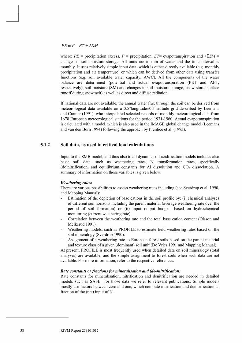
5.1.2 Soil data, as used in critical load calculations
Input to the SMB model, and thus also to all dynamic soil acidification models includes alsobasic soil data, such as weathering rates, N transformation rates, specifically(de)nitrification, and equilibrium constants for Al dissolution and CO2 dissociation. Asummary of information on those variables is given below.
Weathering rates:There are various possibilities to assess weathering rates including (see Sverdrup et al. 1990,and Mapping Manual):- Estimation of the depletion of base cations in the soil profile by: (i) chemical analyses
of different soil horizons including the parent material (average weathering rate over theperiod of soil formation) or (ii) input output budgets based on hydrochemicalmonitoring (current weathering rate).
- Correlation between the weathering rate and the total base cation content (Olsson andMelkerud 1991).
- Weathering models, such as PROFILE to estimate field weathering rates based on thesoil mineralogy (Sverdrup 1990).
- Assignment of a weathering rate to European forest soils based on the parent materialand texture class of a given (dominant) soil unit (De Vries 1991 and Mapping Manual).
At present, PROFILE is most frequently used when detailed data on soil mineralogy (totalanalyses) are available, and the simple assignment to forest soils when such data are notavailable. For more information, refer to the respective references.
Rate constants or fractions for mineralisation and (de-)nitrification:Rate constants for mineralisation, nitrification and denitrification are needed in detailedmodels such as SAFE. For those data we refer to relevant publications. Simple modelsmostly use factors between zero and one, which compute nitrification and denitrification asfraction of the (net) input of N.

RIVM Report 259101012 39
As with the SMB model, in the VSD model complete nitrification is assumed (nitrificationfraction equals 1.0). For the complete soil profile, the nitrification fraction in forest soilsvaries mostly between 0.75 and 1.0. This is based on NH4/NO3 ratios below the rootzone ofhighly acidic Dutch forests with very high NH4 inputs in the early nineties, which werenearly always less than 0.25 (De Vries et al. 1995). Generally, 50% of the NH4 input isnitrified above the mineral soil in the humus layer (Tietema et al. 1990). Actually, thenitrification fraction includes the effect of both nitrification and preferential ammoniumuptake.
Denitrification fractions, which are used in the SMB, VSD and SMART model can berelated to soil type as suggested in Table 3. Ranges are based on data given by Steenvoorden(1984) and Breeuwsma et al. (1991) for peat, clay and sandy soils in the Netherlands. Indeeply drained sandy forest soils, denitrification appears to be nearly negligible(Klemedtson and Svensson 1988).
Table 3: Ranges in denitrification fractions for different soil types.Soil type Denitrification fraction (-)Peat 0.80-0.95Clay 0.7-0.8Sandy/ Loess soils:- with gleyic features 0.4-0.6- without gleyic features 0.0-0.2
Al equilibrium constant and exponent:As in the SMB and SAFE model, Al dissolution is often described by a gibbsite equilibrium.Values for log10Kgibb generally vary between 8.0 and 8.5. In general the Al concentrationdepends upon the H concentration and a site dependent exponent, as given in eq.3.8. Thisdescription is, e.g. used in the VSD, SMART and MAGIC model. Values for KAlox and theexponent a depend on the soil depth.
Especially in forest topsoils, it is more accurate to use values for a that are lower than 3, andconsequently also a different logK value. Regression analyses between the negativelogarithm of the Al concentration (pAl) against the negative logarithm of the Hconcentration (pH), with concentrations in mol.l-1 for nearly 300 Dutch forest stands giveresults as presented in Table 4. The data are based on measurements in approximately 200sandy soils (Leeters and de Vries 2001) and in approximately 40 loess soils, 30 clay soilsand 30 and peat soils (Klap et al. 1999). The results show that the standard gibbsiteequilibrium constant and exponent of 3.0 is reasonable for clay soils. Very different values,however, are required for peat soils and to a lesser extent also for sandy and loess soils,especially at lower soil depths (relevant for multi-layer models such as SAFE).

40 RIVM Report 259101012
Table 4: Estimated values of KAlox and the exponent a based on regression between pAl and pH in thesolution of Dutch soils (Van der Salm and De Vries 2001).Soil type Depth (cm) log KAlox a R2
adj nSandy soils 0-10 -0.56 1.17 56.1 195
10-30 2.37 1.88 82.8 34830-100 5.20 2.51 86.3 172
Peat all depths -1.06 1.31 81.2 116Clay all depths 7.88 2.65 87.3 116Loess 0- 10 -0.48 1.06 64.1 39
10- 30 3.29 1.90 87.9 3930-100 4.55 2.17 92.4 39
Formulae for converting chemical equilibrium constants, such as KAlox, to other units, e.g.from mol/l to eq/m3, can be found in Annex C.
5.1.3 Data needed to simulate cation exchange
In all models, cation exchange is a crucial process. For the VSD model it is the only processincluded in addition to the SMB model. Data needed to allow exchange calculations are:• The pool of exchangeable cations, being the product of layer thickness, bulk density,
cation exchange capacity (CEC) and exchangeable cation fractions• Cation exchange constants (selectivity coefficients)
Preferably these data are taken from measurements. Such measurements generally made forseveral soil horizons. For single-layer models, such as VSD, such data have to be properlyaveraged over the entire soil depth (rooting zone). Formulae for carrying out these averagingare provided in Annex D.
In the absence of measurements, the various data needed to derive the pool of exchangeablecations for major forest soil types can be derived by extrapolation of point data, by usingtransfer functions between bulk density, CEC and base saturation and basic land and soilcharacteristics, such as soil type, soil horizon, organic matter content, soil texture, etc. (DeVries 1991). An overview of such transfer functions and data on soil variables, soilproperties and soil constants is given below. If new data are to be obtained, variousapproaches and analyses methods can be used. This is discussed in Annex E.
Soil bulk density:If no measurements of soil bulk density are available, it can be computed from the followingtransfer function:
(5.1)( )
��
��
�
≥⋅−<<⋅−
≤⋅+⋅+=
%15forlog337.0725.0%15%5for0814.055.1
%5for0015.005.0625.0/1
10 orgorg
orgorg
orgorg
CCCC
CclayCρ
where ρ is the bulk density (g cm-3), Corg is the organic carbon content and clay the claycontent (both in %). The top equation for mineral soils is based on data by Hoekstra andPoelman (1982), the bottom equation for peat(y) soils is derived from Van Wallenburg(1988) and the central equation is a linear interpolation (for clay=0) between the two(Reinds et al. 2001).

RIVM Report 259101012 41
Cation exchange capacity (CEC):The value of the CEC depends on the soil pH at which the measurements are made.Consequently, there is a difference between unbuffered CEC values, measured at the actualsoil pH and buffered values measured at a standard pH, such as 6.5 or 8.2 (see Annex E). Inthe VSD (and many other) models the exchange constants are related to a CEC that ismeasured in a buffered solution in order to standardise to a single pH value (e.g., pH=6.5, asupper limit of non-calcareous soils). The actual CEC can be calculated from pH, clay andorganic carbon content according to (after Helling et al. 1964):
(5.2) orgCpHclaypHpHCEC ⋅−⋅+⋅+⋅= )9.51.5()0.344.0()(
where CEC is the cation exchange capacity (meq/kg), clay is the clay content (%) and Corgthe organic carbon content (%). The pH in this equation should be as close as possible to themeasured soil solution pH. The clay content can be derived from national soil informationsystems or related to the texture class. For sandy soils the clay content can be set to zero ineq.5.2. The organic carbon content of the various soil types can also be derived from thesesources. Values range from 0.1% for arenosols (Qc) to 50% for peat soils (Od). Typicalaverage clay contents as function of the texture class, presented on the FAO soil map, aregiven in Table 5.
Table5: Typical average clay contents and base saturation as a function of soil texture classes.Textureclass
Name Definition Clay content (%) Base saturation (%)
1 coarse clay < 18% and sand ≥ 65% 6 52 medium clay < 35% and sand ≥ 15%;
but clay ≥ 18% if sand ≥ 65%20 15
3 medium fine clay < 35% and sand < 15% 20 204 fine 35% ≤ clay < 60% 45 505 very fine clay ≥ 60% 75 509 organic soils Soil types O 5 10-70
Computing CEC(pHmeasured), i.e. the CEC from eq.5.2, using measured (site-specific) Corg,clay and pH does not always match the measured CEC, CECmeasured, and thus computingCEC at pH=6.5, CEC(6.5), would not be consistent with it. Nevertheless, eq.5.2 can be usedto scale the measured CEC to a value at pH=6.5, i.e. the value needed for modelling, in thefollowing manner:
(5.3) )()5.6(
5.6 measuredpHCECCEC
measuredpH CECCEC ⋅==
This method of scaling measured data with the ratio (or difference) of model output iswidely used in global change work to obtain, e.g., climate-changed (meteorological) dataconsistent with observations.
Exchangeable base cation fraction (base saturation):In most models, a lumped expression is used for the exchange of cations, distinguishingonly between H, Al and base cations (VSD, SMART and SAFE). As with the clay content,data for the exchangeable cation fractions, or in some cases only the base saturation, can bebased on information on national soil information systems, or in absence of these, on theFAO soil map of Europe (FAO 1981). Base saturation data vary from 5-25% in relatively

42 RIVM Report 259101012
acid forest soils to more than 50% in well buffered soils. A very crude indication of the basesaturation as a function of the texture class of soils is given in the last column of Table 5.The relationship in Table 5 is based on data from forest soils given in FAO (1981) and inGardiner (1987). A higher texture class reflects a higher clay content implying an increasein weathering rate, which implies a higher base saturation. For organic soils the initial basesaturation is put equal to 70% for eutric histosols (Oe) and 10% for dystric histosols (Od).
The most preferred method is to use measured CEC and exchangeable cation data. For anational application, such data are, however, often lacking. When data on the initial basesaturation of soils are not available for regional (national) model applications, one mayderive them from a relationship with environmental factors. Such an exercise was carriedout using a European database with approximately 5300 soil chemistry data for the organiclayer and the forest topsoil (0-20 cm) collected on a systematic 16x16 km2 grid (ICP Forestlevel-I grid; Vanmechelen et al. 1997). The regression relationship for the estimated basesaturation EBC (expressed as a fraction with values between 0 and 1) is:
(5.4)
��==
⋅+⋅+
⋅+⋅+⋅+
⋅+⋅+++=���
����
�
−
15
12
11
8
72
65
43210
)fractiondepositionlt()depositionln(
)ionprecipitatln()etemperatur(etemperatur
)ageln(altitude)speciestree()groupsoil(1
ln
kkk
kkk
BC
BC
aa
aaa
aaaaaE
E
where ‘ln’ is the natural logarithm, lt(x)=ln(x/(1-x)), and the ak’s are the regressioncoefficients. The regression analysis was carried out using a so-called Select-procedure.This procedure combines qualitative predictor variables, such as tree species and/or soiltype, with quantitative variables and it combines forward selection, starting with a modelincluding one predictor variable, and backward elimination, starting with a model includingall predictor variables. The ‘best’ model was based on a combination of the percentage ofexplained variance, that should be high and the number of predictor variables that should below.
In the analyses the soils were grouped in ten major FAO soil types (De Vries et al. 1998) butfor this analysis, they were further clustered to four major categories, namely sandy soils,loam/clay soils, peat soils and calcareous soils (not shown here). Results are limited to fourmajor tree species, pine, spruce, oak and beech, which predominate in Northern and CentralEurope. Data on temperature and precipitation are based on interpolations frommeteorological stations for a 10-year period (1985-1996), as an approximation of averagemeteorological conditions. Atmospheric deposition data were derived from EDACS modelcalculations. More information on the procedure is given in Klap et al. (2002). Results ofthe analyses are given in Table 6. The explained variance for base saturation was approx.45%.
Note: When data are not available, one may also calculate base saturation as the maximumof (i) a relation with environmental factors as given above and (ii) an equilibrium withpresent deposition levels of SO4, NO3, NH4 and BC. Especially in southern Europe, whereacid deposition is relatively low and base cation input is high, the base saturation inequilibrium with the present load can be higher than the value computed according to Table6.

RIVM Report 259101012 43
Table 6: Coefficients for estimating base saturation and the C/N-ratio in the mineral topsoil (0-20cm) andthe organic layer (after Klap et al. 2002).Predictor variable Base saturation
(mineral topsoil)
C/N-ratio
organic layer
C/N-ratio
mineral topsoil
Coefficients in
eqs.(5.4) and (5.6)
Constant 3.198 3.115 1.310 a0
Soil group:
Sandy soils 0 0 0 a1
Loamy/clayey soils 0.297 -0.807 -0.279 a1
Peat soils 0.534 -0.025 -0.312 a1
Tree species:
Pine 0 0 0 a2
Spruce -0.113 -0.158 -0.093 a2
Oak 0.856 -0.265 -0.218 a2
Beech 0.591 -0.301 -0.218 a2
Site conditions:
Altitude [m] -0.00014 -0.00008 -0.000136 a3
Age [yr] 0 0.025 0.096 a4
Meteorology:
Temperature [°C] 0 -0.0078 -0.041 a5
Temperature2 [°C2] 0 0.00095 0.0014 a6
Precipitation [mm/yr] 0 0.178 0.194 a7
Deposition:
Na [eq/ha/yr] -0.223 0 0.080 a8
N-tot (=NOy+NHz) [eq/ha/yr]:
Sandy soils 0 -0.150 -0.019 a9
Loamy/clayey soils 0 -0.032 0 a9
Peat soils 0 -0.136 0 a9
Acid (=SOx-ssca) + N-tot) [eq/ha/yr] -1.025 0 0 a10
Bc-ssca) (=Ca+Mg+K-ssc) [eq/ha/yr] 0.676 0 0 a11
Deposition fractions:
NHz / Acid [-]:
Sandy soils 0 0 0 a12
Loamy/clayey soils -0.494 0 0 a12
Peat soils -0.896 0 0 a12
NHz / N-tot [-] 0 0.102 0.120 a13
Ca-ssca) / Bc-ssc [-] 1.211 0 0 a14
Mg-ssca) / Bc-ssc [-] 0.567 0 0 a15
a) ssc = sea salt corrected; if <0.1, set =0.1 to avoid underflow in the equations.
Other exchangeable cation fractions:Separate exchangeable base cation fractions (as needed in the MAGIC model) could not bederived from environmental factors, as described above, since data were not available. Thesame holds for Al, which is a crucially important exchangeable cation. Thus a relationshipwas derived between the exchangeable Al fraction, EAl, and the base saturation, EBc, basedon data in the sandy, loess and clay soils described above (De Vries and Leeters 2001,Leeters and De Vries 2001, Klap et al. 1999). The fitted relationship is:

44 RIVM Report 259101012
(5.5)))(exp(1 MEB
CAEBc
Al −−++=
with the coefficients given in Table 7.
Table 7: Coefficients describing the relationship between exchangeable Al fraction and base saturation.Soil group A C B M R2-adj (%)Sand 0.01236 17.73 -5.117 -0.7562 59Loess -0.07161 37.32 -2.877 -1.385 82Clay 0.00031 0.22731 -13.65 0.33769 86All soils -0.0028 0.4414 -7.54 0.2194 63
Exchange constants:In most exchange models the cations are lumped to H, Al and base cations (VSD, SMARTand SAFE), but in MAGIC every base cation (Ca, Mg, K, Na) is modelled separately.Furthermore, cation exchange in SMART and MAGIC is based upon Gaines-Thomasequations, in SAFE it is described by Gapon exchange reactions, whereas in the VSD modelthe user can chose between the two. Exchange constants can be derived from thesimultaneous measurement of the major cations (H, Al, Ca, Mg, K and Na) on theadsorption complex and in the soil solution.
Decadic logarithms of average exchange constants thus derived for sand, loess, clay andpeat soils with their standard deviations (‘stddev’), are given in the Tables below. As withthe Al dissolution data, the data are based on measurements in approximately 200 sandysoils (Leeters and De Vries 2001) and in approximately 40 loess soils, 30 clay soils and 30and peat soils (Klap et al. 1999). The tables show the high affinity of the complex forprotons compared to all other monovalent cations. The relative contributions of K, Na andNH4 on the adsorption complex are very low. Formulae for the conversion of units areprovided in Annex C. A detailed overview over data sources, calculation methods andconnections/correlations between the various exchange constants can be found in De Vriesand Posch (2003).
Results for the exchange constants needed in the VSD model (in ‘Gaines-Thomas mode’)are given in the Tables 8 and 9. The exchange constants needed in this model are onlyrelated to the exchange between H and Bc=Ca+Mg+K and between Al and Bc.
Table 8: Mean and standard deviation of logarithmic Gaines-Thomas exchange constants of H againstCa+Mg+K as a function of soil depth for sand, loess, clay and peat soils (mol/l)-1.Layer Sand Loess Clay Peat(cm) Mean stddev Mean stddev Mean stddev Mean stddev0-10 5.338 0.759 5.322 0.692 6.740 1.464 4.754 0.50210-30 6.060 0.729 5.434 0.620 6.007 0.740 4.685 0.57330-60 6.297 0.656 - - 6.754 0.344 5.307 1.05160-100 6.204 0.242 5.541 0.579 7.185 - 5.386 1.6360-30 5.236 0.614 5.386 0.606 6.728 1.373 4.615 0.4390-60 5.863 0.495 - - 6.887 1.423 4.651 0.562

RIVM Report 259101012 45
Table 9: Mean and standard deviation of logarithmic Gaines-Thomas exchange constants of Al againstCa+Mg+K as a function of soil depth for sand, loess, clay and peat soils (mol/l).Layer Sand Loess Clay Peat(cm) Mean stddev Mean stddev Mean stddev Mean stddev0-10 2.269 1.493 1.021 1.147 1.280 1.845 0.835 1.20410-30 3.914 1.607 1.257 0.939 -0.680 1.152 0.703 0.96830-60 4.175 1.969 - - -3.070 0.298 0.567 1.47460-100 2.988 0.763 1.652 1.082 -2.860 - 0.969 1.7770-30 2.306 1.082 0.878 1.079 0.391 1.555 0.978 0.8050-60 2.858 1.121 - - -0.973 1.230 0.666 0.846
Results for the exchange constants needed in the SMART model are given in Tables 10 and11. The exchange constants needed in this model are related to the exchange between H andCa+Mg, Al and Ca+Mg.
Table 10: Mean and standard deviation of logarithmic Gaines-Thomas exchange constants of H againstCa+Mg as a function of soil depth for sand, loess, clay and peat soils (mol/l)-1.Layer Sand Loess Clay Peat(cm) Mean stddev Mean stddev Mean stddev Mean stddev0-10 5.200 0.779 5.306 0.704 6.703 1.500 4.573 0.54910-30 5.968 0.715 5.474 0.587 5.999 0.740 4.579 0.57630-60 6.249 0.660 - - 6.734 0.344 5.243 1.04260-100 6.393 0.249 5.519 0.553 7.155 - 5.343 1.6270-30 5.136 0.607 5.391 0.590 6.709 1.391 4.487 0.4680-60 5.739 0.513 - - 6.876 1.430 4.575 0.583
Table 11: Mean and standard deviation of logarithmic Gaines-Thomas exchange constants of Al againstCa+Mg as a function of soil depth for sand, loess, clay and peat soils (mol/l).Layer Sand Loess Clay Peat(cm) Mean. stddev Mean. stddev Mean. stddev Mean. stddev0-10 1.856 1.557 0.974 1.154 1.170 1.781 0.294 1.23010-30 3.639 1.517 1.376 1.045 -0.703 1.182 0.385 1.01630-60 4.029 1.853 - - -3.128 0.298 0.376 1.54260-100 3.553 0.899 1.586 1.100 -2.951 - 0.840 1.7610-30 2.004 1.057 0.892 1.158 0.334 1.521 0.592 0.8590-60 2.486 1.008 - - -1.005 1.252 0.437 0.902
Results for the exchange constants needed in the MAGIC model are given in the Tables 12-15. Note that the exchange of protons against Al or base cations is not included in theMAGIC model. It should be noted, however, that in the MAGIC model activities are usedinstead of concentrations. In an earlier version of MAGIC (Cosby et al. 1985) another, butequivalent, set of exchange equations had been used.
Table 12: Mean and standard deviation of logarithmic Gaines-Thomas exchange constants of Al againstCa as a function of soil depth for sand, loess, clay and peat soils (mol/l).Layer Sand Loess Clay Peat(cm) Mean stddev Mean stddev Mean stddev Mean stddev0-10 1.630 1.581 0.931 1.194 1.080 1.814 0.072 1.24210-30 3.287 1.542 1.395 1.122 -0.812 1.216 0.197 0.99830-60 3.654 2.100 - - -3.253 0.432 0.154 1.52760-100 3.545 1.084 1.677 1.179 -3.329 - 0.560 1.7420-30 1.719 1.058 0.860 1.193 0.206 1.515 0.392 0.8400-60 2.010 1.094 - - -1.125 1.292 0.216 0.886

46 RIVM Report 259101012
Table 13: Mean and standard deviation of logarithmic Gaines-Thomas exchange constants of Al againstMg as a function of soil depth for sand, loess, clay and peat soils (mol/l).Layer Sand Loess Clay Peat(cm) Mean stddev Mean stddev Mean stddev Mean stddev0-10 2.346 1.637 1.116 1.071 1.478 1.727 0.805 1.40310-30 3.995 1.588 1.373 0.965 -0.391 1.116 0.935 1.24930-60 4.378 1.791 - - -2.841 0.022 1.010 1.74260-100 3.583 0.670 1.509 1.032 -1.866 - 1.340 1.9760-30 2.554 1.008 1.022 1.091 0.783 1.573 1.131 1.0700-60 3.142 1.031 - - -0.594 1.195 1.024 1.154
Table 14: Mean and standard deviation of logarithmic Gaines-Thomas exchange constants of Al against Kas a function of soil depth for sand, loess, clay and peat soils (mol/l)2.Layer Sand Loess Clay Peat(cm) Mean stddev Mean stddev Mean stddev Mean stddev0-10 -1.065 1.086 -2.637 1.032 -2.931 1.664 -1.228 0.97710-30 -0.398 1.144 -2.498 0.972 -4.288 0.749 -0.944 0.57830-60 -0.676 1.494 - - -5.162 0.319 -0.887 0.94060-100 -2.670 0.880 -1.715 0.912 -4.653 - -0.639 1.3490-30 -0.876 0.816 -2.678 0.848 -3.539 1.548 -0.888 0.5050-60 -0.838 0.868 - - -4.426 0.706 -0.910 0.522
Table 15: Mean and standard deviation of logarithmic Gaines-Thomas exchange constants of Al againstNa as a function of soil depth for sand, loess, clay and peat soils (mol/l)2.Layer Sand Loess Clay Peat(cm) Mean stddev Mean stddev Mean stddev Mean stddev0-10 1.268 1.170 1.783 1.016 1.338 0.925 0.822 0.95810-30 2.496 1.313 0.335 1.568 0.107 0.633 0.836 0.60430-60 2.310 1.500 - - -0.538 0.053 0.922 0.89160-100 1.064 0.374 -0.796 1.301 0.024 - 0.879 1.0600-30 1.977 0.827 0.996 1.287 1.264 0.942 1.089 0.5920-60 2.181 0.819 - - 0.732 0.787 0.944 0.569
Finally, the Gapon exchange constants for the cations used in VSD (in ‘Gapon mode’) andSAFE are given in the Tables 16-17. Beware of the different units of the exchange constantscompared to the Gaines-Thomas equations due to a different description of the exchangeprocess (see eqs.3.11-3.14).
Table 16: Mean and standard deviation of logarithmic Gapon exchange constants of H against Ca+Mg+Kas a function of soil depth for sand, loess, clay and peat soils (mol/l)-1/2.Layer Sand Loess Clay Peat(cm) Mean stddev Mean stddev Mean stddev Mean stddev0-10 3.178 0.309 3.138 0.268 3.684 0.568 2.818 0.19910-30 3.527 0.271 3.240 0.221 3.287 0.282 2.739 0.17530-60 3.662 0.334 - - 3.521 0.212 2.944 0.38260-100 3.866 0.125 3.232 0.251 3.676 - 3.027 0.6720-30 3.253 0.311 3.170 0.206 3.620 0.530 2.773 0.1900-60 3.289 0.340 - - 3.604 0.654 2.694 0.170

RIVM Report 259101012 47
Table 17: Mean and standard deviation of logarithmic Gapon exchange constants of Al against Ca+Mg+Kas a function of soil depth for sand, loess, clay and peat soils (mol/l)1/6.Layer Sand Loess Clay Peat(cm) Mean stddev Mean stddev Mean stddev Mean stddev0-10 0.306 0.440 0.190 0.546 -0.312 0.738 -0.373 0.35010-30 0.693 0.517 0.382 0.663 -0.463 0.431 -0.444 0.25530-60 0.819 0.527 - - -1.476 0.093 -0.740 0.33660-100 1.114 0.121 0.390 0.591 -1.795 - -0.867 0.4010-30 0.607 0.472 0.221 0.647 -0.609 0.731 -0.247 0.4040-60 0.199 0.633 - - -1.054 0.362 -0.551 0.210
Note that exchange constants are not independent (see eqs. 3.12 and 3.13). For example, themean of the logarithm of the Gapon exchange constant for H-Al exchange can be obtainedby subtracting a value in Table 17 from the respective value in Table 16. These and otherformulae relating the different exchange constants can be found in De Vries and Posch(2003).
5.1.4 Data needed to include balances for nitrogen, sulphate and aluminium
C/N-ratio:As with CEC and base saturation, data for the C/N-ratio of soils should preferably be basedon measurements. For national applications, it can also be based on information on nationalsoil information systems, or in absence of this on the FAO soil map of Europe (FAO 1981).Data for the C/N-ratio generally vary between 15 in rich soils where humification has beenhigh to 40 in soils with low N inputs and less humification. Values can also be obtainedfrom results of a regression analysis similar to that of the base saturation according to:
(5.6)
( )
��==
⋅+⋅+
⋅+⋅+⋅+
⋅+⋅+++=
15
12
11
8
72
65
43210
)fractiondepositionlt()depositionln(
)ionprecipitatln()etemperatur(etemperatur
)ageln(altitude)speciestree()groupsoil(ratio-C/Nln
kkk
kkk aa
aaa
aaaaa
where lt(x) = ln(x/(1-x)). Results of the analysis, which was performed with the same datasets as described in the section on base saturation, are given in Table 6. As with the basesaturation, more information on the procedure is given in Klap et al. (2002).
Sorption capacity and half-saturation constant for sulphate:Values for the maximum sorption capacity for sulphate, Smax, can be related to the content ofoxalate extractable Al (meq kg-1) according to (Johnson and Todd 1983):
(5.7) oxmax AlS ⋅= 02.0
Estimates for the oxalate extractable Al content are given below. Adsorption or half-saturation constants for sulphate, S1/2, can be derived from literature information (e.g. Singhand Johnson 1986, Foster et al. 1986). A reasonable average value is 1.0 eq/m3.
Al-hydroxide content:Data for the oxalate extractable Al content (the content of readily available Al-hydroxide)are available in several national soil information systems, such as the soil information

48 RIVM Report 259101012
system of the Netherlands. In sandy soils the Al-hydroxide content (in meq/kg) mostlyvaries between 100-200 for A-horizons, between 200-350 for B-horizons and between 50-150 for C-horizons (parent material, De Vries 1991).
Moisture content:In any dynamic model, which includes a mass balance for elements, information on the soilmoisture content is needed. An approximation of the annual average soil moisture content canbe made as a function of the clay content according to (Brady 1972):
(5.8) clay⋅+= 0077.004.0θ
This equation holds for clay contents up to 30%. Above 30% a constant value of 0.27 isassumed.
5.2 Model calibration
If all input parameters, initial conditions and driving forces were known, the chosen modelwould describe the future development of the soil chemical status for any given depositionscenario. However, in most cases several of the parameters are poorly known, and thus manymodels, i.e. the badly known parameters in the model, have to be ‘calibrated’. The method ofcalibration varies with the model and/or the application.
In standard applications of both the MAGIC and SAFE model it is assumed that in pre-acidification times (say 1850) the input of ions is in equilibrium (steady state) with the soil(solution) chemistry. Furthermore it is assumed that the deposition history of all (eight) ions isknown (properly reconstructed).
In SAFE, weathering rates and uptake/net removal of N and base cations are computed withinthe model (see above). Only simulated present base saturation is matched with observations (inevery soil layer) by adjusting the cation exchange selectivity coefficient(s). Matching simulatedand observed soil solution concentrations is not part of the standard calibration procedure.
The calibration of MAGIC is a sequential process whereby firstly the input and output ofthose ions assumed to act conservatively in the catchment are balanced (usually only Cl).Next, the anion concentrations in surface waters are matched by adjusting catchment netretention (of N) and soil adsorption (of S) if appropriate. Thirdly, the four individual majorbase cation concentration in the stream and on the soil solid phase (expressed as apercentage of cation exchange capacity) are matched by adjusting the cation exchangeselectivity coefficients and the base cation weathering rates. Finally, surface water pH, Aland organic anion concentrations are matched by adjusting the aluminium solubilitycoefficient and total organic acid concentration in surface water.
Both in MAGIC and SAFE automatic calibration routines are part of the overall model system.For the SMART and VSD model no such automatic model calibration routines are presentlyavailable. To date, in site-specific applications calibration has been carried out by ‘trial anderror’, and in European applications the initial base saturation in 1960 has been derived fromtransfer functions, thus avoiding any calibration and the reconstruction of historic (pre-1960)depositions.

RIVM Report 259101012 49
6 Model Calculations and Presentation of ModelResults
6.1 Model calculations, especially target loads
For every model, the most demanding part is not the actual running of the model, but thederivation and preparation of input data (files) and the model initialisation/calibration. Forregional applications, i.e. runs for many sites, additional work is usually required to embed themodel – designed for a single site – into a suitable (data base) framework which allows theefficient handling of model inputs and outputs.
As outlined above (section 2.3), target loads, or target load functions in the case of acidification,are a feasible way to interact with integrated assessment models, not least due to their similaritywith critical load functions. The computation of target loads is not straightforward. Afterspecifying the target year and the year of implementation of the (yet unknown) target load, thedynamic model has to be run iteratively, until the deposition (= target load) is found which isrequired for the soil to reach the desired chemical status in the specified target year. Thefollowing examples demonstrate the different cases that can arise when calculating target loadsand what can happen when doing such calculation ‘blindly’. For simplicity we use a singledeposition, but the conclusions hold for target load functions as well.
As an example, Figure 6 shows the deposition history (left) and the resulting molar Al/Bc-ratio (right) as simulated (by the VSD model) for three different soils, characterised by theirCEC (40, 60 and 80 meq/kg). In two cases the Al/Bc-ratio at ‘present’ (year 2010) is abovethe critical value (=1), while for CEC=80 it stayed below it during the past.
1970 1990 2010 2030 2050 20700
100
200
300
400
500
600
700
800
year
Dep
(eq
/ha/
yr)
CEC=40
CEC=60
CEC=80
1970 1990 2010 2030 2050 20700
0.25
0.50
0.75
1.00
1.25
1.50
1.75
2.00
year
Al/B
c (m
ol/m
ol)
Figure 6: Temporal development of acidifying deposition (left) and corresponding molar Al/Bc-ratio (right) for 3 soils varying in CEC. The two vertical lines separate 50 years of ‘history’, 10years (2010-2020) of implementation, and the future. Also shown are the critical load and thecritical value (Al/Bc)crit=1 as thin horizontal lines. The deposition drops to the critical load withinthe implementation period and the Al/Bc-ratios (slowly) approach the critical value.

50 RIVM Report 259101012
To investigate the future behaviour of the soils, we let the deposition drop to the critical load(which is independent of the CEC) during the ‘implementation decade’ (marked by twovertical lines in Figure 6). Obviously, for CEC=80, the Al/Bc-ratio stays below one,whereas for CEC=60 it drops below one within the first decade and then slowly rises againtowards the critical value. For CEC=40, the Al/Bc-ratio stays well above the critical value,approaching it asymptotically over time. In all three cases the approach to the critical valueis very slow.
Next we look at target load calculations for these three soils. Figure 7 shows the results oftarget load calculations for 40 years, i.e. achieving (Al/Bc)crit=1 in the year 2050. ForCEC=40 meq/kg the target load is smaller than the critical load, as one would expect. ForCEC=60 and 80, however, the computed target loads are higher than the critical load. AsFigure 7 illustrates, this does not make sense: After reaching the critical limit, these twosoils deteriorate and the Al/Bc-ratio gets larger and larger. Since target loads are supposedto protect also after the target year, we stipulate that whenever a calculated target load ishigher than the critical load, it has to be set equal to the critical load.
CEC=40
CEC=60
CEC=80
1970 1990 2010 2030 2050 20700
100
200
300
400
500
600
700
800
year
Dep
(eq
/ha/
yr)
CEC=40
CEC=60
CEC=80
1970 1990 2010 2030 2050 20700
0.25
0.50
0.75
1.00
1.25
1.50
1.75
2.00
year
Al/B
c (m
ol/m
ol)
Figure 7: Target loads (with 2050 as target year) for three soils and the resulting Al/Bc-ratio(left). Note that for CEC=60 and 80 the target load is higher than the critical load, even when(Al/Bc)crit<1 at present (for CEC=80)! Clearly, in such cases target load calculations don’t makesense.
In the light of the above considerations we define that a target load is the deposition for whicha pre-defined chemical or biological status is reached in the target year and maintained (orimproved) thereafter.
In view of this, the calculation of a target load should be carried out as depicted by the flowchart in Figure 8.

RIVM Report 259101012 51
Exceedance of CL in 2010?
Yes No
No
Yes NoRun model with "zero"deposition until target year
Run model with 2010deposition until target year
Al/Bc>1 in target year?
Al/Bc>1 in 2010?
Al/Bc>1 in target year?
Compute TL
Yes
Target cannot be achieved No deposition reductions needed
No
Run model with CLuntil target year
Al/Bc>1 in target year?
TL = CL
Yes
NoYes
Figure 8: Flow chart of the procedure to calculate a target load, avoiding the pitfalls mentioned inthe text (e.g. computing a target load that allows violation of the criterion after the target year).
The first check at every site is, whether the critical load (CL) is exceeded in the reference year(2010 in our case). If the answer is ‘yes’ (as for the soils with CEC=40 and 60 in Fig.6), thenext step is to run the dynamic model with the deposition equal to the critical load. If in thetarget year the chemical criterion is no longer violated (e.g. Al/Bc≤1), the target load equals thecritical load (TL=CL).
If, after running the model with the critical load as deposition, the criterion is still violated in thetarget year, the model has to be run with “zero” deposition until the specified target year.“Zero” deposition means a deposition small enough as not to contribute to acidification (oreutrophication). In the case of nitrogen this would mean that Ndep is set equal to CLmin(N), thusavoiding problems, e.g. negatively influencing forest growth in case of zero N deposition.
If, after running the model with “zero” deposition, the criterion is still violated in the targetyear, then the target cannot be met in that year. In such a case recovery can only be achieved in

52 RIVM Report 259101012
a later year. Otherwise, a target load exists and has to be calculated; its value lies somewherebetween zero and the critical load.
If the critical load is not (or no longer) exceeded in 2010 (as for the soil with CEC=80 in Fig.6),this does not mean that the risk of damage to the ecosystem is already averted – it only meansthat eventually, maybe after a very long time, the chemical criterion is no longer violated. Onlyif, in addition, the chemical criterion is not violated in 2010, no further emission reductions arerequired for that ecosystem. Also, if the model is run with the 2010 deposition until the targetyear and the criterion is no longer violated in that year, no further emission reductions arerequired. If the criterion is still violated in the target year, the procedure continues with runningthe model with “zero” deposition etc (see Figure 8).
In the implementation of the above procedure one could skip the step in which the model is runwith the critical load as deposition (in case of exceedance in 2010) and immediately start withtarget load calculations (if a target load exists). And only afterwards check if this target load isgreater than CL (and set it to CL) (see soil with CEC=60 in Fig.7). However, in view of the factthat TL calculations require iterative model runs, and also to avoid surprises due to round-offerrors, it makes good sense to include that intermediate step.
An issue requiring attention in all target load calculations is the assumptions about finitenitrogen buffers. If it is, e.g., assumed that a soil can immobilise N for (say) the next 50years to a larger degree than assumed in the critical load calculations, then target loads willalways be higher than the critical load. This might cause confusion and demands carefulexplanations.
When summarising target load calculations for ecosystems in a grid square (or region) it isimportant not only to report those sites for which target load (functions) have been derived,but all three cases (and their areas), i.e. the sites for which (i) no further depositionreductions are necessary, (ii) a target load has been calculated, and (iii) no target load exists(for the given target year). Note that in case (i), the 2010 deposition has necessarily to bebelow (or equal to) the critical load.
6.2 Presentation of model results
For single site applications of dynamic models the obvious way to present model output aregraphs of the temporal development of the most relevant soil chemical variables, such as basesaturation or the concentrations of ions in the soil solution (e.g. Al/Bc-ratio), in response togiven deposition scenarios. In regional (European) applications, however, this kind ofinformation has to be summarised. This can be done in several ways, e.g., by displaying thetemporal development of selected percentiles of the cumulative distribution of the variable(s) ofinterest (see Figure 9 and, e.g., Kurz et al. 1998). Another way is to show a sequence of mapsdisplaying the variable of interest in (say) five-year intervals (‘map movies’). Other options arediscussed and illustrated in Evans et al. (2001) and Jenkins et al. (2002).

RIVM Report 259101012 53
5%50%75%90%
95%
1920 1960 2000 2040 20804.0
4.5
5.0
5.5
6.0
6.5
year
pH
Figure 9: Example of percentile traces of a regional dynamic model output (Kurz and Posch 2002).From it 7 percentiles (5, 10, 25, 50, 75, 90 and 95%) can be read for every time step.
Maps can represent single sites only if their number does not become too large. If the number ofsites reaches the thousands, statistical descriptors (means, percentiles) have to be used torepresent the model output. For example, for a given target year the percentage of ecosystemsin a grid square for which the target is reached under a given deposition scenario can bedisplayed in a map format, very much in the same way as protection percentages (derived fromprotection isolines) have been displayed for critical load exceedances. The procedures forcalculating percentiles and ‘target load’ isolines can be found in Posch et al. (1995) and theMapping Manual.

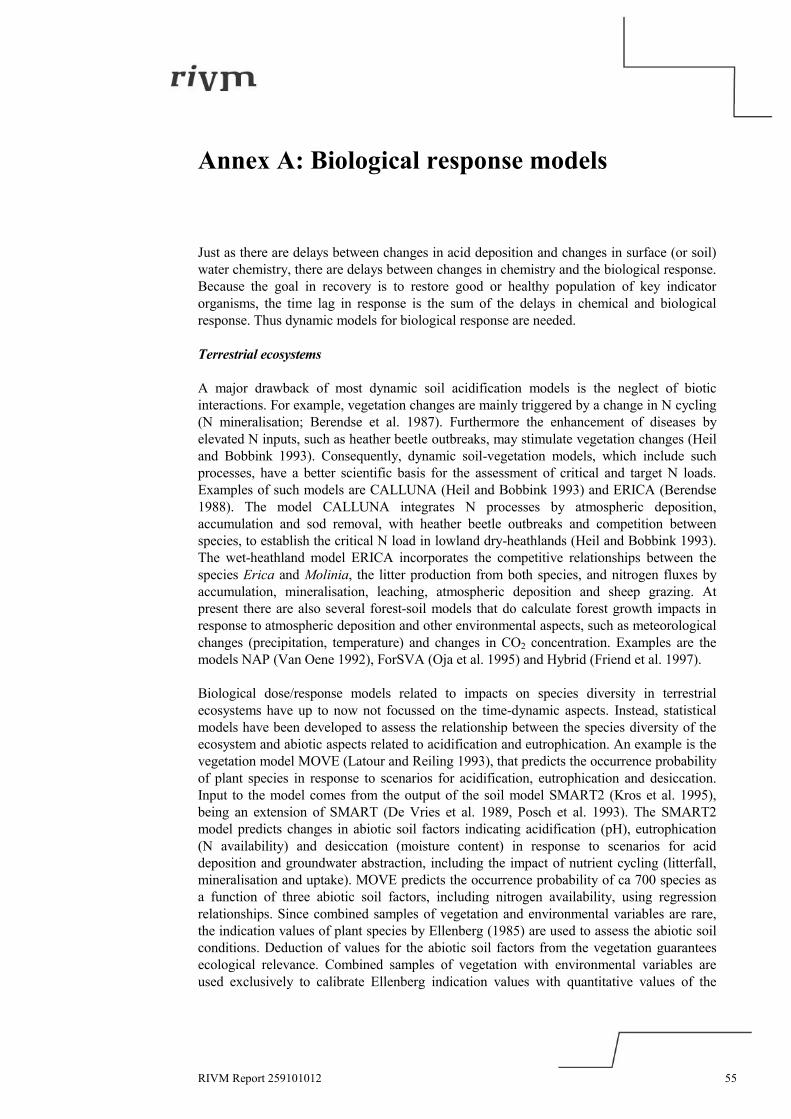
RIVM Report 259101012 55
Annex A: Biological response models
Just as there are delays between changes in acid deposition and changes in surface (or soil)water chemistry, there are delays between changes in chemistry and the biological response.Because the goal in recovery is to restore good or healthy population of key indicatororganisms, the time lag in response is the sum of the delays in chemical and biologicalresponse. Thus dynamic models for biological response are needed.
Terrestrial ecosystems
A major drawback of most dynamic soil acidification models is the neglect of bioticinteractions. For example, vegetation changes are mainly triggered by a change in N cycling(N mineralisation; Berendse et al. 1987). Furthermore the enhancement of diseases byelevated N inputs, such as heather beetle outbreaks, may stimulate vegetation changes (Heiland Bobbink 1993). Consequently, dynamic soil-vegetation models, which include suchprocesses, have a better scientific basis for the assessment of critical and target N loads.Examples of such models are CALLUNA (Heil and Bobbink 1993) and ERICA (Berendse1988). The model CALLUNA integrates N processes by atmospheric deposition,accumulation and sod removal, with heather beetle outbreaks and competition betweenspecies, to establish the critical N load in lowland dry-heathlands (Heil and Bobbink 1993).The wet-heathland model ERICA incorporates the competitive relationships between thespecies Erica and Molinia, the litter production from both species, and nitrogen fluxes byaccumulation, mineralisation, leaching, atmospheric deposition and sheep grazing. Atpresent there are also several forest-soil models that do calculate forest growth impacts inresponse to atmospheric deposition and other environmental aspects, such as meteorologicalchanges (precipitation, temperature) and changes in CO2 concentration. Examples are themodels NAP (Van Oene 1992), ForSVA (Oja et al. 1995) and Hybrid (Friend et al. 1997).
Biological dose/response models related to impacts on species diversity in terrestrialecosystems have up to now not focussed on the time-dynamic aspects. Instead, statisticalmodels have been developed to assess the relationship between the species diversity of theecosystem and abiotic aspects related to acidification and eutrophication. An example is thevegetation model MOVE (Latour and Reiling 1993), that predicts the occurrence probabilityof plant species in response to scenarios for acidification, eutrophication and desiccation.Input to the model comes from the output of the soil model SMART2 (Kros et al. 1995),being an extension of SMART (De Vries et al. 1989, Posch et al. 1993). The SMART2model predicts changes in abiotic soil factors indicating acidification (pH), eutrophication(N availability) and desiccation (moisture content) in response to scenarios for aciddeposition and groundwater abstraction, including the impact of nutrient cycling (litterfall,mineralisation and uptake). MOVE predicts the occurrence probability of ca 700 species asa function of three abiotic soil factors, including nitrogen availability, using regressionrelationships. Since combined samples of vegetation and environmental variables are rare,the indication values of plant species by Ellenberg (1985) are used to assess the abiotic soilconditions. Deduction of values for the abiotic soil factors from the vegetation guaranteesecological relevance. Combined samples of vegetation with environmental variables areused exclusively to calibrate Ellenberg indication values with quantitative values of the

56 RIVM Report 259101012
abiotic soil factors. A calibration of these indication values to quantitative values of theabiotic soil factors is necessary to link the soil module to the vegetation module.
A comparable statistical model is the NTM model (Schouwenberg et al. 2000), that wasdeveloped to predict the potential conservation value of natural areas. Normally conservationvalues are calculated on the basis of plant species or vegetation types. As with MOVE, NTMhas the possibility to link the vegetation and the site conditions by using plant ecologicalindicator values. NTM uses a matrix of the habitats of plant species defined on the basis ofmoisture, acidity and nutrient availability. The model was calibrated using a set of 160,252vegetation relevees. A value index per plant species was defined on the basis of rarity, declineand international importance. This index was used to determine a conservation value for eachrelevee. The value per relevee was then assigned to each species in the relevee and regressed onthe Ellenberg indicator values for moisture, acidity and nutrient availability (Ellenberg 1985)using a statistical method (P-splines). The model has these three Ellenberg indication values asinput for the prediction of the potential conservation value. A potential conservation value iscalculated for a combination of the abiotic conditions and vegetation structure (ecotope).Therefore four vegetation types are accounted for, each represented by a submodel of NTM:heathland, grassland, deciduous forest and pine-forest. Use of those models in dynamicmodelling assessments is valuable to gain more insight in the effect of deposition scenarios onterrestrial ecosystems.
Aquatic ecosystems
As with terrestrial ecosystems, biological dose/response models for surface waters have notgenerally focussed on the time-dynamic aspects. For example, the relationship between lakeANC and brown trout population status in Norwegian lakes used to derive the critical limitin the Mapping Manual is based on synoptic (once in time) surveys of ANC and fish statusin a large number of lakes. Similarly the invertebrate indices (Raddum 1999) and diatomresponse models (Allot et al. 1995, Battarbee et al. 1996) do not incorporate time-dynamicaspects. Additional information on dose/response comes from traditional laboratory studiesof toxicity (chronic and acute) and reproductive success.
Information on response times for various organisms comes from studies of recoveryfollowing episodes of pollution, for example, salmon population following chemical spill ina river. For salmon full recovery of the population apparently requires about 10 years afterthe water chemistry has been restored.
There are currently no available time-dynamic process-oriented biological response modelsfor effects of acidification on aquatic and terrestrial organisms, communities or ecosystems.Such models are necessary for a full assessment of the length of time required for recoveryof damage from acidification.
There are several types of evidence that can be used to empirically estimate the time delaysin biological recovery. The whole-lake acidification and recovery experiments conducted atthe Experimental Lakes Area (ELA), north-western Ontario, Canada, provide suchinformation at realistic spatial and temporal scales. These experiments demonstrateconsiderable lag times between achievement of acceptable water quality following decreasein acid inputs, and achievement of acceptable biological status. The delay times for variousorganisms are at least several years. In the case of several fish species irreversible changesmay have occurred (Hann and Turner 2000, Mills et al. 2000).

RIVM Report 259101012 57
A second source of information on biological recovery comes from liming studies. Over theyears such studies have produced extensive empirical evidence on rate of response ofindividual species as well as communities following liming. There has been little focus,however, on the processes involved.
Finally there is recent documentation of recovery in several regions at which acid depositionhas decreased in the 1980s and 1990s. Lakes close to the large point-source of sulphuremissions at Sudbury, Ontario, Canada, show clear signs of chemical and biologicalrecovery in response to substantial decreases in emissions beginning in the late 1970s(Keller and Gunn 1995). Lakes in the nearby Killarney Provincial Park also show clearsigns of biological recovery during the past 20 years (Snucins et al. 2001). Here there areseveral biological factors that influence the rate of biological recovery such as:(1) fish species composition and density(2) dispersal factors such as distance to intact population and ability to disperse(3) existence of resting eggs (for such organisms such as zooplankton)(4) existence of precluding species – i.e. the niche is filled.Recently, a workshop held under the auspices of the UNECE reviewed the currentknowledge on models for biological recovery in surface waters (see Wright and Lie 2002).
Future work on biological response models must also include consideration of the frequencyand severity of harmful episodes, such as pH shocks during spring snowmelt, or acidity andaluminium pulses due to storms with high seasalt inputs. These links between episodic waterchemistry and biological response at all levels (organisms, community, and ecosystem) arepoorly quantified and thus not yet ready to be incorporated into process-oriented models.

58 RIVM Report 259101012
Annex B: Base saturation as a critical limit
Finite buffers, such as cation exchange capacity and its base saturation, are not considered inthe derivation of critical loads, since they do not influence steady-state situations. However, thisdoes not mean that the state of those buffers is not influenced by the steady state! Therelationship between the base saturation, EBc, and the Al/Bc-ratio can be easily derived for theBc-Al-H exchange system. When using Gaines-Thomas equations, inserting EAl and EH fromeqs.3.12 into eq.3.15 and using eq.3.8 (see section 3.2) to express [H] in terms of [Al]yields:
(B1) 1][][ /12/1/1
2/1/12/1
2/1
2/12/3 =++ − αα
α
BcKAlKr
EBcKr
EEox
HBceqBc
AlBceqBcBc
where req=[Al]/[Bc] is the equivalent Al/Bc-ratio. This cubic equation in EBc1/2 can easily be
solved numerically to obtain the base saturation as function of the (critical) Al/Bc-ratio(Figure Ba). As can be seen, for average values of the equilibrium constants and a widerange of base cation concentrations ([Bc]=(Bcdep+Bcw-Bcu)/Q in steady state), the widely-used value of (Al/Bc)crit=1 corresponds to very low (steady-state) base saturation values. Thesame picture emerges when using the Gapon exchange model. In this case the equations canbe solved explicitly for the base saturation:
(B2)
αα
α
/12/1/1
/1
6/1
3/1
][][1
1
−++=
BcKAlkr
Bckr
E
ox
HBceqAlBceqBc
and in Figure Bb it is shown as function of the (critical) molar Al/Bc-ratio.
Figure B indicates that the path to steady state can lead to a substantial loss of the pool ofexchangeable base cations. This could be at odds with ensuring the overall viability of forestsand forest soils, and a critical (acceptable, minimum) base saturation could be chosen as acriterion for calculating critical acidity loads in order to avoid (large) losses of base cations (seeHall et al. 2001, UNECE 2001b). It is also interesting to note that base saturation is used ascriterion in the New England Governors/Eastern Canadian Premiers ‘Acid Rain ActionPlan’ for calculating sustainable S and N depositions to upland forests with the SMB model(NEG/ECP 2001).

RIVM Report 259101012 59
0 0.5 1.0 1.5 2.00
2
4
6
8
10
(Al/Bc)crit (mol/mol)
base
sat
urat
ion
(%)
Gaines-Thomas
0 0.5 1.0 1.5 2.00
2
4
6
8
10
(Al/Bc)crit (mol/mol)
base
sat
urat
ion
(%)
Gapon
Figure B: Base saturation as a function of the (critical) molar Al/Bc-ratio for 4 different basecation concentrations ([Bc]= 20 (lowest curve), 50, 100 and 200 meq/L (highest curve); α=3 andKAlox=108 (mol/L)–2). (a) For the Gaines-Thomas exchange equations (KAlBc=1 mol/L, KHBc=105
(mol/L)–1), and (b) for Gapon exchange equations (kAlBc=10 (mol/L)1/6 , kHBc=10 (mol/L)–1/2).

60 RIVM Report 259101012
Annex C: Unit conversions
For convenience we use the term ‘equivalents’ (eq) instead of the SI-unit ‘moles of charge’(molc). If X is an ion with molecular weight M and charge z, then one has:
(C1) XeqXmol1X g 1Mz
M==
Obviously, moles and equivalents are the same for z=1.
When dealing with equations of chemical equilibria, the unpleasant task of converting theequilibrium constants to the required units often arises. In the following we give a formulawhich should cover most of the cases encountered: Let A and B be two chemicalcompounds in the following equilibrium equation:
(C2) ynxm K ]B[ = ]A[ ±±
where the square brackets [...] denote concentrations in mol/L (L stands for litre), implyingfor the equilibrium constant K the units (mol/L)x-y. If the concentrations are to be expressedin eq/V, where V is an arbitrary volume unit with 1L=10cV, then the equilibrium constant inthe new units is given by
(C3) yxy
xxyc
nmK = K −−⋅ )eq/V(10' )(
Note: To convert to mol/V, set m=n=1 in the above equation; and to covert to g/V setm=1/MA and n=1/MB, where MA and MB are the molecular weights of A and B, resp.
Example 1: The gibbsite equilibrium is given by [Al3+]=K[H+]3, i.e. m=3, x=1, n=1, y=3and (e.g.) K=108(mol/L)-2. To convert to eq/m3, one has c=–3 and thus K ' = 108 ⋅10–3·(3–1) ⋅3= 300 (eq/m3)–2.
The above reasoning can also be used for converting exchange constants. For example, theGapon equation for Al-Bc exchange can be written as
(C4) 3/132/12 ][][ ++ = AlkBcEE
AlBcBc
Al
and since exchangeable fractions are dimensionless, eq.C3 can be used.
Example 2: Let log10kAlBc=0; then kAlBc=100=1(mol/L)1/6 (x=1/2, y=1/3). Since m=2 and n=3,one gets when converting to eq/m3, i.e. c=–3, kAlBc=1⋅10–3·(1/3–1/2) ⋅(21/2/31/3) = 3.100806(eq/m3)1/6.And for kHBc the multiplier to obtain (eq/m3)–1/2 is 0.0021/2=0.0447213.

RIVM Report 259101012 61
Annex D: Averaging soil profile properties
For single layer soil models, such as VSD, SMART or MAGIC, the profile averages of certainsoil parameters are required. In the following we give the formulae for the average bulk densityρ (g/cm3), cation exchange capacity CEC (meq/kg) and base saturation EBC.
For a given soil profile we assume that there are measurements of bulk density ρl cationexchange capacity CECl and base saturation EBC,l for n (homogeneous) soil horizons withthickness zl (l=1,..., n). Obviously, the total thickness (soil depth) z is given by
(D1) �=
=n
llzz
1
and the mean bulk density ρ of the profile is derived from mass conservation (per unit area):
(D2) �=
=n
lllz
z 1
1 ρρ
The average cation exchange capacity CEC has to be calculated in such a way that the totalnumber of exchange sites (per unit area) is given by z⋅ρ⋅CEC. This implies the followingformula for the profile average cation exchange capacity:
(D3) �=
=n
llll CECz
zCEC
1
1 ρρ
And for the average base saturation of the profile we get then:
(D4) �=
=n
llBClllBC ECECz
CECzE
1,
1 ρρ
NB: For aquatic ecosystems, these parameters have to be averaged over the catchment area aswell.

62 RIVM Report 259101012
Annex E: Measuring techniques for soil data
An overview of the various measuring methods that can be used when gathering new soildata is given in Table E-1. The data are arranged according to their importance.
Table E-1: Measuring techniques for soil dataVariable Measuring techniquesCEC Extraction with NH4-acetate buffered at pH 6.5 or 0.01 N AgTu unbufferedEBC
1 Extraction with an unbuffered solution e.g., i.e. BaCl2
EAl ibidρ Sampling a fixed volume and weightingClt Kurmies method (wet digestion)Nlt Kjeldahl method (wet digestion)KXY Centrifugation of a soil sample in which H, Al, Ca, Mg, K, Na and NH4 are measured at the
adsorption complex and in the soil solutionCacb Wesemael method (weight loss) or Scheibler method (CO2 evolution)Alox Etraction with NH4-oxalate buffered at pH 5.5Smax Adding SO4 at a concentration of 200 mg/l and extraction of the amount at the complex with
0.016 N NaH2PO41 BC (Ca, Mg, K and Na) can also be measured in a buffered solution
The cation exchange capacity should be measured in a buffered solution in order tostandardise to one pH value. There are two possibilities in this respect: use ofbariumchloride - tri-ethanolamine (BaCl2-TEA) buffered at pH 8.2 or ammonium - acetate(NH4OAC) buffered at pH 6.5. Since cation exchange plays a major role in non-calcareoussoils with a maximum pH near 6.5, the NH4OAC method is used. The principle of thismethod is the measurement of the NH4 concentration after percolation (column experiment)or shaking (batch experiment) of a soil sample with a solution of a known NH4 concentra-tion. The removal of NH4 is equal to the CEC.
The base cation fraction at the adsorption complex can be measured in the ammonium -acetate percolate. However, in order to measure the Al fraction at the adsorption complex, itis necessary to use an unbuffered solution. In this respect there are various possibilities,including an unbuffered BaCl2 method. The concentrations of Al, Ca, Mg (and possibly Naand K) in the percolate are measured by atomic emission (ICP) or atomic adsorptionspectrophotometry (AAS). The fraction of H at the adsorption complex is derived by sub-tracting the sum of Al, Ca, Mg, K and Na from the CEC.
The carbonate content of the soil can be measured by adding a strong acid (generally HCl)and measuring the weight loss or the CO2 evolution of the soil sample. The first method(Wesemeal) is fast but less accurate, whereas the second method (Scheibler) is timedemanding but more accurate.
The amount of Al in hydroxides which buffer the acid lead can be extracted by variousmethods e.g. pyrophosphate, ammonium-oxalate and dithionite. The second method isrecommended since laboratory experiments indicate that this gives a good indication of thereactive amount of Al.

RIVM Report 259101012 63
Carbon and nitrogen in litter can be determined after wet digestion using a mixture of H2O2.Total C and total N can than be determined by the Kurmies and Kjeldahl methodrespectively.
Exchange constants for H and Al versus Ca+Mg (BC) can be derived by measuring theconcentrations of H, Ca, Mg and Al in the soil solution, which can be extracted bycentrifugation. This should be done in samples where the amount at the adsorption complexis also measured. In this way, exchange constants have been derived for different layers(horizons) of acid sandy soils in the Netherlands (Kleijn et al. 1989).
Measurement of Smax requires a laboratory experiment, which is rather time-consuming. Theprinciple of this method is described in Johnson and Todd (1983).


RIVM Report 259101012 65
References
Alcamo J, Shaw R, Hordijk L (eds) (1990) The RAINS Model of Acidification − Scienceand Strategies in Europe. Kluwer Academic Publishers, Dordrecht, The Netherlands,402 pp.
Allott TEH, Battarbee RW, Curtis C, Kreiser AM, Juggins S, Harriman R (1995) Anempirical model of critical acidity loads for surface waters based onpalaeolimnological data. In: Hornung M, Sutton MA, Wilson RB (eds) Mapping andModelling of Critical Loads for Nitrogen: A Workshop Report. Institute of TerrestrialEcology, Penicuik, United Kingdom, pp.50-54.
Alveteg M, Sverdrup H, Warfvinge P (1995) Regional assessment of the temporal trends insoil acidification in southern Sweden, using the SAFE model. Water, Air and SoilPollution 85: 2509-2514.
Alveteg M (1998) Dynamics of forest soil chemistry. PhD thesis, Reports in Ecology andEnvironmental Engineering 3:1998, Department of Chemical Engineering II, LundUniversity, Lund, Sweden, 81 pp.+appendices.
Alveteg M, Walse C, Warfvinge P (1998a) A method for reconstructing historic depositionand uptake from present day values. Water, Air and Soil Pollution 104: 269-283.
Alveteg M, Sverdrup H, Kurz D (1998b) Integrated assessment of soil chemical status. 2.Application of a regionalized model to 622 forested sites in Switzerland. Water, Airand Soil Pollution 105: 11-20.
Alveteg M, Posch M, Sverdrup H, Warfvinge P (2000) Calculating isolines of partialecosystem recovery. Poster presented at the ‘Acid rain 2000’ Conference, Tsukuba,Japan.
Alveteg M, Sverdrup H (2002) Manual for regional assessments using the SAFE model(draft version 8 April 2002). Department of Chemical Engineering II, LundUniversity, Lund, Sweden. www2.chemeng.lth.se
Battarbee RW, Allott TEH, Juggins S, Kreiser AM, Curtis C, Harriman R (1996) Criticalloads of acidity to surface waters - an empirical diatom-based palaeolimnologicalmodel. Ambio 25: 366-369.
Berendse F, Beltman B, Bobbink R, Kwant M, Schmitz MB (1987) Primary production andnutrient availability in wet heathland ecosystems. Acta Oec./Oecol. Plant. 8: 265-276.
Berendse F (1988) The nutrient balance of vegetation on dry sandy soils in the context ofeutrophication via the air. Part 1: A simulation model as an aid for the management ofwet heathlands (in Dutch). Centre for Agrobiological Research, Wageningen, TheNetherlands, 51 pp.
Breeuwsma A, Chardon JP, Kragt JF, De Vries W (1991) Pedotranfer functions fordenitrification. In: ECE, Soil and Groundwater Research Report II: Nitrate in Soils,Commission of the European Communities, Luxembourg, pp. 207-215.

66 RIVM Report 259101012
Cosby BJ, Hornberger GM, Galloway JN, Wright RF (1985a) Modeling the effects of aciddeposition: Assessment of a lumped parameter model of soil water and streamwaterchemistry. Water Resources Research 21(1): 51-63.
Cosby BJ, Wright RF, Hornberger GM, Galloway JN (1985b) Modeling the effects of aciddeposition: Estimation of long-term water quality responses in a small forestedcatchment. Water Resources Research 21(11): 1591-1601.
Cosby BJ, Hornberger GM, Galloway JN, Wright RF (1985c) Time scales of catchmentacidification: A quantitative model for estimating freshwater acidification.Environmental Science & Technology 19:1144-1149.
Cosby BJ, Hornberger GM, Wright RF, Galloway JN (1986) Modeling the effects of aciddeposition: Control of long-term sulfate dynamics by soil sulfate adsorption. WaterResources Research 22(8): 1283-1291.
Cosby BJ, Hornberger GM, Wright RF (1989) Estimating time delays and extent of regionalde-acidification in southern Norway in response to several deposition scenarios. In: JKämäri, DF Brakke, A Jenkins, SA Norton, RF Wright (eds) Regional AcidificationModels: Geographic Extent and Time Development. Springer Verlag, New York, pp.151-166.
Cosby BJ, Wright RF, Gjessing E (1995) An acidification model (MAGIC) with organicacids evaluated using whole-catchment manipulations in Norway. Journal ofHydrology 170: 101-122.
Cosby BJ, Ferrier RC, Jenkins A, Emmett BA, Wright RF, Tietema A (1997) Modelling theecosystem effects of nitrogen deposition: Model of Ecosystem Retention and Loss ofInorganic Nitrogen (MERLIN). Hydrology and Earth System Sciences 1:137-158.
Cosby BJ, Ferrier RC, Jenkins A, Wright RF (2001) Modelling the effects of aciddeposition: refinements, adjustments and inclusion of nitrogen dynamics in theMAGIC model. Hydrology and Earth System Sciences 5(3): 499-517.
De Vries W, Posch M, Kämäri J (1989) Simulation of the long-term soil response to aciddeposition in various buffer ranges. Water, Air and Soil Pollution 48: 349-390.
De Vries W, Hol A, Tjalma S, Voogd JC (1990) Stores and residence times of elements in aforest ecosystem: a literature study (in Dutch). DLO-Staring Centrum, Rapport 94,Wageningen, The Netherlands, 205 pp.
De Vries W (1991) Methodologies for the assessment and mapping of critical loads and theimpact of abatement strategies on forest soils. DLO Winand Staring Centre forIntegrated Land, Soil and Water Research, Report 46, Wageningen, The Netherlands,109 pp.
De Vries W (1994) Soil response to acid deposition at different regional scales. Field andlaboratory data, critical loads and model predictions. PhD Thesis, AgriculturalUniversity, Wageningen, The Netherlands, 487 pp.
De Vries W, Reinds GJ, Posch M, Kämäri J (1994) Simulation of soil response to acidicdeposition scenarios in Europe. Water, Air and Soil Pollution 78: 215-246.
De Vries W, Van Grinsven JJM, Van Breemen N, Leeters EEJM, Jansen PC (1995) Impactsof acid atmospheric deposition on concentrations and fluxes of solutes in Dutch forestsoils. Geoderma 67: 17-43.

RIVM Report 259101012 67
De Vries W, Reinds GJ, Deelstra HD, Klap JM, Vel EM (1998) Intensive Monitoring ofForest Ecosystems in Europe, Technical Report 1998. UNECE, EC, Forest IntensiveMonitoring Coordinating Institute, 193 pp.
De Vries W, Leeters EEJM (2001) Chemical composition of the humus layer, mineral soiland soil solution of 150 forest stands in the Netherlands in 1990. Alterra-rapport424.1, Alterra Green World Research, Wageningen, The Netherlands, 114 pp.
De Vries W, Posch M (2003) Derivation of cation exchange constants for sand loess, clayand peat soils on the basis of field measurements in the Netherlands. Alterra-rapport701, Alterra Green World Research, Wageningen, The Netherlands, 50 pp.
Dise NB, Matzner E, Gundersen P (1998) Synthesis of nitrogen pools and fluxes fromEuropean forest ecosystems. Water, Air and Soil Pollution 105: 143-154.
Ellenberg H (1985) Veränderungen der Flora Mitteleuropas unter dem Einfluss vonDüngung und Immissionen. Schweizerische Zeitschift für das Forstwesen 136: 19-39.
Evans C, Jenkins A, Helliwell R, Ferrier R, Collins R (2001) Freshwater Acidification andRecovery in the United Kingdom. Centre for Ecology and Hydrology, Wallingford,United Kingdom, 80 pp.
FAO (1981) FAO-Unesco Soil Map of the World, 1:5,000,000. Volume V Europe. Unesco,Paris 1981, 199 pp.
Foster NW, Morrison IK, Nicolson JA (1986) Acid deposition and ion leaching from apodzolic soil under hardwood forest. Water, Air and Soil Pollution 31: 879-889.
Friend AD, Stevens AK, Knox RG, Channel MGR (1997) A process-based terrestrialbiosphere model of ecosystem dynamics (Hybrid v3.0). Ecological Modelling 95:249-287.
Gardiner MJ (1987) Representative data for major soil units in the EEC soil map. An ForasTaluntais, Ireland. Internal Report, 486 pp.
Gundersen P, Emmett BA, Kjonaas OJ, Koopmans CJ, Tietema A (1998a) Impact ofnitrogen deposition on nitrogen cycling in forests: a synthesis of NITREX data.Forest Ecology and Management 101: 37-55.
Gundersen P, Callesen I, De Vries W (1998b) Nitrate leaching in forest ecosystems iscontrolled by forest floor C/N ratio. Environmental Pollution 102: 403-407.
Hall J, Ashmore M, Curtis C, Doherty C, Langan S, Skeffington R (2001) UN/ECE expertworkshop: Chemical criteria and critical limits. In: Posch et al. (2001) op. cit., pp. 67-71.
Hann BJ, Turner MA (2000) Littoral microcrustacea in Lake 302S in the ExperimentalLakes Area of Canada: acidification and recovery. Freshwater Biology 43: 133-146.
Heil GW, Bobbink R (1993) ‘CALLUNA’ a simulation model for evaluation of impacts ofatmospheric nitrogen deposition on dry heathlands. Ecological Modelling 68: 161-182.
Helling CS, Chesters G, Corey RB (1964) Contribution of organic matter and clay to soilcation exchange capacity as affected by the pH of the saturating solution. Soil Sci.Soc. Am. J. 28: 517-520.

68 RIVM Report 259101012
Hettelingh J-P, Posch M (1994) Critical loads and a dynamic assessment of ecosystemrecovery. In: J Grasman, G van Straten (eds) Predictability and Nonlinear Modellingin Natural Sciences and Economics. Kluwer Academic Publishers, Dordrecht, TheNetherlands, pp. 439-446.
Hoekstra C, Poelman JNB (1982) Density of soils measured at the most common soil typesin the Netherlands (in Dutch). Report 1582, Soil Survey Institute, Wageningen, TheNetherlands, 47 pp.
Jenkins A, Larssen T, Moldan F, Posch M, Wright RF (2002) Dynamic modelling of surfacewaters: Impact of emission reduction – possibilities and limitations. ICP-WatersReport 70/2002, Norwegian Institute for Water Research (NIVA), Oslo, Norway, 42pp.
Johnson DW, Todd DE (1983) Relationships among iron, aluminium, carbon, and sulfate ina variety of forest soils. Soil Sci. Soc. Am. J. 47: 792-800.
Kämäri J, Posch M (1987) Regional application of a simple lake acidification model toNorthern Europe. In: MB Beck (ed) Systems Analysis in Water Quality Management,Pergamon Press, Oxford, pp. 73-84.
Kauppi P, Kämäri J, Posch M, Kauppi L, Matzner E (1986) Acidification of forest soils:Model development and application for analyzing impacts of acidic deposition inEurope. Ecological Modelling 33: 231-253.
Keller W, Gunn JM (1995) Lake water quality improvements and recovering aquaticcommunities. In: Gunn JM (ed), Restoration and Recovery of an Industrial Region,Springer Verlag, New York, pp.67-80.
Klap JM, De Vries W, Leeters EEJM (1999) Effects of acid atmospheric deposition on thechemical composition of loess, clay and peat soils under forest in the Netherlands.Report 97, DLO Winand Staring Centre for Integrated Land, Soil and WaterResearch, Wageningen, The Netherlands.
Klap JM, Brus DJ, De Vries W, Reinds GJ (2002) Assessment of site-specific estimates ofcritical deposition levels for nitrogen and acidity in European forest ecosystems usingmeasured and interpolated soil chemistry. (in prep).
Kleijn CE, Zuidema G, De Vries W (1989) The indirect effects of atmospheric depositionon the vitality of Dutch forest. 2. Deposition, soil properties and soil solutioncomposition of eight Douglas stands (in Dutch). Report 2050, Soil Survey Institute,Wageningen, The Netherlands, 92 pp.
Klemedtson L, Svensson BH (1988) Effects of acid deposition on denitrification and N2Oemission from forest soils. In: J Nilsson, P Grennfelt (eds) Critical loads for sulphurand nitrogen. Nord 1988:97, Nordic Council of Ministers, Copenhagen, Denmark,pp.343-362.
Kros J, Reinds GJ, De Vries W, Latour JB, Bollen M (1995) Modelling of soil acidity andnitrogen availability in natural ecosystems in response to changes in acid depositionand hydrology. Report 95, DLO Winand Staring Centre, Wageningen, TheNetherlands, 90 pp.
Kurz D, Alveteg M, Sverdrup H (1998) Integrated assessment of soil chemical status. 1.Integration of existing models and derivation of a regional database for Switzerland.Water, Air and Soil Pollution 105: 1-9.

RIVM Report 259101012 69
Kurz D, Posch M (2002) A comparison of the SAFE and VSD soil dynamic models usingSwiss data. Report of a collaborative study, CCE, Bilthoven, The Netherlands, 32 pp.
Latour JB, Reiling R (1993) A multiple stress model for vegetation (MOVE): a tool forscenario studies and standard setting. Science of the Total Environment Supplement93: 1513-1526.
Leemans R, Cramer W (1991) The IIASA database for mean monthly values oftemperature, precipitation and sunshine on a global terrestrial grid. IIASA ReseachReport RR-91-18, International Institute of Applied System Analysis, Laxenburg,Austria, 61 pp.
Leemans R, Van den Born GJ (1994) Determining the potential distribution of vegetation,crops and agricultural productivity. Water, Air and Soil Pollution 76: 133-161.
Leeters EEJM, De Vries W (2001) Chemical composition of the humus layer, mineral soiland soil solution of 200 forest stands in the Netherlands in 1995. Alterra-rapport424.2, Alterra Green World Research, Wageningen, The Netherlands, 108 pp.
Martinson L, Alveteg M, Warfvinge P (2003) Parameterization and evaluation of sulfateadsorption in a dynamic soil chemistry model. Environmental Pollution 124(1): 119-125.
Mills KH, Chalanchuk SM, Allan DJ (2000) Recovery of fish populations in Lake 223 fromexperimental acidification. Can. J. Fish. Aquat. Sci. 57: 192-204.
NEG/ECP (2001) Protocol for Assessment and Mapping of Forest Sensitivity toAtmospheric S and N Deposition, prepared by the NEG/ECP Forest Mapping Group,New England Governors/Eastern Canadian Premiers, ‘Acid Rain Action Plan 2001,Action Item 4: Forest Mapping Research Project’, 79 pp.
Oja T, Yin X, Arp PA (1995) The forest modelling series ForM-S: applications to theSolling spruce site. Ecological Modelling 83: 207-217.
Olsson M, Melkerud PA (1991) Determination of weathering rates based on geochemicalproperties of the soil. In: E Pulkinen (ed) Environmental geochemistry in NorthernEurope. Geological Survey of Finland, Special paper 9, pp.69-78.
Posch M, Reinds GJ, De Vries W (1993) SMART - A Simulation Model for Acidification'sRegional Trends: Model description and user manual. Mimeograph Series of theNational Board of Waters and the Environment 477, Helsinki, Finland, 43 pp.
Posch M, De Smet PAM, Hettelingh J-P, Downing RJ (eds) (1995) Calculation andMapping of Critical Thresholds in Europe. Status Report 1995, Coordination Centerfor Effects, National Institute of Public Health and the Environment (RIVM),Bilthoven, The Netherlands, iv+198 pp. www.rivm.nl/cce/
Posch M, De Vries W (1999) Derivation of critical loads by steady-state and dynamic soilmodels. In: SJ Langan (ed) The Impact of Nitrogen Deposition on Natural and Semi-Natural Ecosystems. Kluwer Academic Publishers, Dordrecht, The Netherlands, pp.213-234.
Posch M, De Smet PAM, Hettelingh J-P, Downing RJ (eds) (2001) Modelling and mappingof critical thresholds in Europe. Status Report 2001, Coordination Center for Effects,National Institute for Public Health and the Environment (RIVM), Bilthoven, TheNetherlands, iv+188 pp. www.rivm.nl/cce

70 RIVM Report 259101012
Posch M, Reinds GJ (2003) VSD - User Manual of the Very Simple Dynamic soilacidification model. Coordination Center for Effects, National Institute for PublicHealth and the Environment (RIVM), Bilthoven, The Netherlands (in preparation).
Prentice IC, Sykes MT, Cramer W (1993) A simulation model for the transient effects ofclimate change on forest landscapes. Ecological Modelling 65: 51-70.
Raddum GG (1999) Large scale monitoring of invertebrates: Aims, possibilities andacidification indexes. In: GG Raddum, BO Rosseland, J Bowman (eds) Workshop onBiological Assessment and Monitoring; Evaluation and Models. ICP-Waters Report50/99, Norwegian Institute for Water Research, Oslo, Norway, pp.7-16.
Reinds GJ, Posch M, De Vries W (2001) A semi-empirical dynamic soil acidification modelfor use in spatially explicit integrated assessment models for Europe. Alterra Report084, Alterra Green World Research, Wageningen, The Netherlands, 55 pp.
Reuss JO (1980) Simulation of soil nutrient losses due to rainfall acidity. EcologicalModelling 11: 15-38.
Reuss JO (1983) Implications of the calcium-aluminum exchange system for the effect ofacid precipitation on soils. Journal of Environmental Quality 12(4): 591-595.
Reuss JO, Johnson DW (1986) Acid Deposition and the Acidification of Soils and Waters.Ecological Studies 59, Springer, New York, 119 pp.
SAEFL (1998) Acidification of Swiss forest soils - Development of a regional dynamicassessment. Environmental Documentation No.89, SAEFL, Berne, Switzerland, 115pp.
Singh BR, Johnson DW (1986) Sulfate content and adsorption in soils of two forestedwatersheds in southern Norway. Water, Air and Soil Pollution 31: 847-856.
Schouwenberg EPAG, Houweling H, Jansen MJW, Kros J, Mol-Dijkstra JP (2000)Uncertainty propagation in model chains: a case study in nature conservancy. AlterraReport 001, Alterra Green World Research, Wageningen, The Netherlands, 90pp.
Snucins S, Gunn JM, Keller W, Dixit S, Hindar A, Henriksen A (2001) Effects of regionalreductions in sulphur deposition on the chemical and biological recovery of lakeswithin Killarney Park, Ontario, Canada. Journal of Environmental Monitoring andAssessment 67: 179-194.
Starr M (1999) WATBAL: A model for estimating monthly water balance components,including soil water fluxes. In: S Kleemola, M Forsius (eds) 8th Annual Report,UNECE ICP Integrated Monitoring, Finnish Environment Institute, Helsinki, Finland.The Finnish Environment 325: 31-35. www.metla.fi/hanke/3098/info-en.htm
Steenvoorden J (1984) Effects of changes in water management on water quality (in Dutch).Report 1554, Institute for Land and Water Management, Wageningen, TheNetherlands.
Sverdrup HU (1990) The kinetics of base cation release due to chemical weathering. LundUniversity Press, Lund, Sweden, 246 pp.
Sverdrup H, De Vries W, Henriksen A (1990) Mapping Critical Loads. NORD 1990:98,Nordic Council of Ministers, Copenhagen, Denmark, 124 pp.

RIVM Report 259101012 71
Sverdrup H, De Vries W (1994) Calculating critical loads for acidity with the Simple MassBalance model. Water, Air and Soil Pollution 72: 143-162.
Tietema A, Duysings JJHM, Verstraten JM, Westerveld JW (1990) Estimation of actualnitrification rates in an acid forest soil. In: AF Harrison, P Ineson, OW Heal (eds)Nutrient cycling in terrestrial ecosystems; Field methods, application andinterpretation. Elsevier Applied Science, London and New York, pp.190-197.
Tiktak A, Van Grinsven JJM (1995) Review of sixteen forest-soil-atmosphere models.Ecological Modelling 83: 35-53.
UBA (1996) Manual on Methodologies and Criteria for Mapping Critical Levels/Loads andGeographical Areas Where They Are Exceeded, Texte 71/96. Umweltbundesamt,Berlin, Germany, 144+lxxiv pp. www.icpmapping.com/
Ulrich B (1981) Ökologische Gruppierung von Böden nach ihrem chemischenBodenzustand. Z. Pflanzenernähr. Bodenk. 144: 289-305.
UNECE (1999) Report of the seventeenth session of the Executive Body. DocumentECE/EB.AIR/68, United Nations Economic Commission for Europe, Geneva, 61 pp.
UNECE (2001a) Expert group meeting on dynamic modelling. DocumentEB.AIR/WG.1/2001/11, United Nations Economic Commission for Europe, Geneva,6 pp.
UNECE (2001b) Workshop on chemical criteria and critical limits. DocumentEB.AIR/WG.1/2001/13, United Nations Economic Commission for Europe, Geneva,8 pp.
Van der Salm C, De Vries W (2001) A review of the calculation procedure for critical acidloads for terrestrial ecosystems. Science of the Total Environment 271: 11-25.
Vanmechelen L, Groenemans R, Van Ranst E (1997) Forest soil condition in Europe.Results of a Large-Scale Soil Survey. EC-UN/ECE, Brussels, Geneva, 261 pp.
Van Oene H (1992) Acid deposition and forest nutrient imbalances: a modelling approach.Water, Air and Soil Pollution 63: 33-50.
Van Wallenburg C (1988) The density of peaty soils (in Dutch). Internal Report, SoilSurvey Institute, Wageningen, The Netherlands, 5 pp.
Warfvinge P, Sverdrup H (1992) Calculating critical loads of acid deposition withPROFILE - A steady-state soil chemistry model. Water, Air and Soil Pollution 63:119-143.
Warfvinge P, Holmberg M, Posch M, Wright RF (1992) The use of dynamic models to settarget loads. Ambio 21: 369-376.
Warfvinge P, Falkengren-Grerup U, Sverdrup H, Andersen B (1993) Modelling long-termcation supply in acidified forest stands. Environmental Pollution 80: 209-221.
Wright RF, Lie MC (eds) (2002) Workshop on models for biological recovery fromacidification in a changing climate, 9-11 September 2002 in Grimstad, Norway. AcidRain Research Report 55/02, Norwegian Institute for Water Research (NIVA), Oslo,Norway, 42 pp.