Embed Size (px)
Citation preview

Manual Calibration
University of Oklahoma/HyDROSModule 2.2

Module 2.2 / Manual Calibration
Outline – Day 2
- 2 -
RAINFALL AND PETMANUAL CALIBRATION• Description of EF5/CREST
parameters• Description of EF5/KW parameters• Manual calibration strategies• Distributed vs. lumped parameters• Calibrate EF5 for Okavango River
AUTOMATIC CALIBRATIONINTERPRETING AND USING MODEL OUTPUT

Module 2.2 / Manual Calibration
Manual Calibration
- 3 -
What is calibration?
Calibration is the process of adjusting model parameters so that the model more accurately simulates stream flow (as compared to observed stream flow)
We adjust each parameter and see how the model evaluation indices (NSCE, CC, and bias) change
This can be a lengthy and complex process – there is no one right answer when it comes to calibration

Module 2.2 / Manual Calibration
EF5 Parameters
- 4 -
First, let’s review what we know about EF5’s parameters
There are a total of 13 of themThey’re divided into 2 categories• The CREST parameters, which affect the water balance
(how water is partitioned and accounted for in each cell)• The kinematic wave parameters, which affect how water
is routed from cell to cell
Some parameters affect the model results more than others
WM, B, ALPHA, BETA, and ALPHA0 are generally the most important, but others can be too

Module 2.2 / Manual Calibration
CREST Parameters
- 5 -
The CrestParamSet block contains the six water balance parameters
• WMMaximum soil water capacity
• PBThe exponent of the variable infiltration curve
• IMImpervious area ratio
• KEConversion factor from PET to actual ET
• FCSoil saturated hydraulic conductivity
• IWUInitial value of soil water, a % of WM
CREST Water
Balance
WM B
IM
KE FC
IWU

Module 2.2 / Manual Calibration
WM
- 6 -
WM is the maximum soil water capacity (depth integrated pore space) of the soil layer in the model, in millimeters
This is how much water the soil layer can storePhysically, this a function of several soil propertiesIf I increase WM, that means there’s more space in the soil for water, which means less runoff will be produced
WM will generally be between 5.0 and 250.0 mm
WM

Module 2.2 / Manual Calibration
B
- 7 -
B
B is the exponent of the variable infiltration curve (VIC)
Remember the VIC governs how much water enters the soil layer and how much remains at the surface as runoffIf I increase B, I tend to produce more runoff
B can range between 0.1 and 20.0

Module 2.2 / Manual Calibration
IM
- 8 -
IM
IM is the impervious area ratioYou can think of this as the percentage area of your modeled domain covered in roofs, concrete, rocky soils and other impervious materialsIf I increase IM, my runoff increases
IM can range from nearly 0 to 0.5
You generally do NOT want to calibrate IM, because it is fairly easy to observe from surveys or remote sensing
So if you know 10% of a basin is covered in rocks or concrete, your IM should be about 0.10
VEGETATION IMPERVIOUS

Module 2.2 / Manual Calibration
KE
- 9 -
KE
KE is the multiplier to convert between input PET and local actual ET
This is essentially an adjustment to the monthly global PET grid to make it more accurately reflect conditions over the modeled basin
The PET forcing provided in this training course tends to be a little too “hot”
In other words, too much water gets evaporated when the original PET grid values are used
KE can range from 0.001 (one one-thousandth of the PET grid) to 1.0 (the entire PET grid)
You can use values over 1.0, but this worsens the already “hot” tendency of the provided PET grids

Module 2.2 / Manual Calibration
FC
- 10 -
FC is the soil saturated hydraulic conductivity (Ksat) in mm/hr
This describes how easily water moves through saturated soilThe higher the value, the more easily water can travel through saturated soilsHigher values tend to decrease runoffFC can be determined from soil properties and field measurements, which can help reduce the possible range of values in the calibration process
FC can range from 0.0 to 150.0 Guide for estimating Ksat from soil, from NSSH Part 618 (Subpart B),
NRCS, USDA
FC
Module 2.2 / Manual Calibration
IWU
- 11 -
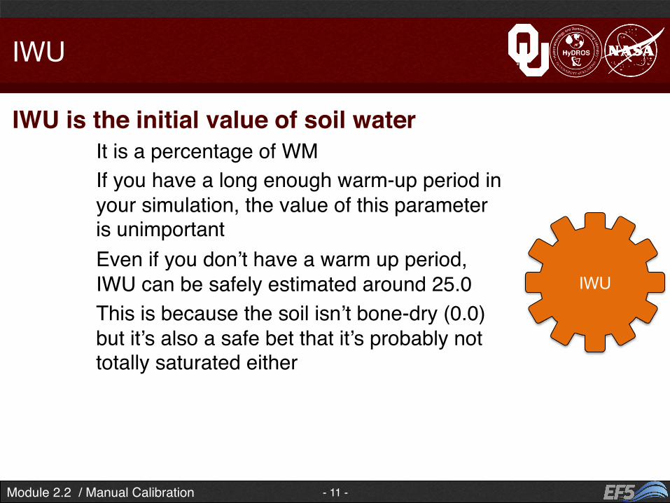
IWU is the initial value of soil waterIt is a percentage of WMIf you have a long enough warm-up period in your simulation, the value of this parameter is unimportantEven if you don’t have a warm up period, IWU can be safely estimated around 25.0This is because the soil isn’t bone-dry (0.0) but it’s also a safe bet that it’s probably not totally saturated either
IWU

Module 2.2 / Manual Calibration
CREST Parameter Summary
- 12 -
To summarize:WM and B are important to the accuracy of the simulation, so focus your attention here when calibratingFC and IM can be measured or estimated for a basin via other means, so pick values for these and leave them aloneIWU is not important if you use a warm-up periodKE should generally be less than 1.0 when using the PET grids provided with this training
CREST Water
Balance
WM B
IM
KE FC
IWU

Module 2.2 / Manual Calibration
Routing Parameters
- 13 -
Kinematic Wave
Routing
LEAKI ISU
UNDER
TH BETA
ALPHA
ALPHA0
The KWParamSet block contains the seven routing parameters in EF5
• THNumber of grid cells needed to flow into a cell for it to be part of a channel
• UNDERThe interflow flow speed multiplier
• LEAKIAmount of water leaked from interflow reservoir in each time step
• ISUInitial value of the interflow reservoir
• ALPHA and BETAUsed in the equation Streamflow = alpha*(cross-sectional channel area)beta
• ALPHA0The alpha value used for overland, not channel, routing

Module 2.2 / Manual Calibration
TH
- 14 -
TH is the threshold for how many cells must drain into a cell for it to become part of a river in the model
• Determined from the FAC grid
• Dependent on resolution of the topographical files
• As the FAC resolution increases, the value of TH should also increase
If you convert from grid cells to actual area (in km2), TH should be between 30 and 300 km2
1 5 3 2 1 1 2 6 3 2 1 2 3 9 1 2 1 3 3 15 18 20 4 1 2 2 2 31 5 2 1 1 1 36 4 3
TH

Module 2.2 / Manual Calibration
UNDER
- 15 -
UNDER is the interflow flow speed multiplier
• Higher values of this mean water moves faster through the soil layer, which can result in faster peaks in a hydrograph
• This only affects the timing of the flood wave, not the volume of water making it into the river channel
This parameter can range between 0.0001 and 3.0
UNDER
Interflow
INTERFLOW RESERVOIR

Module 2.2 / Manual Calibration
LEAKI
- 16 -
LEAKI is the amount of water leaking out of the interflow reservoir at each time step
• This is expressed as a percentage of the total water in the interflow reservoir
• The water that leaks out moves on to the next downstream cell’s interflow reservoir
• Increasing this parameter will result in faster peaks
This can range between 0.01 and 1.0
LEAKI
Interflow
INTERFLOW RESERVOIR

Module 2.2 / Manual Calibration
ISU
- 17 -
ISU is the initial value of the interflow reservoir
• If you use a warm-up period this parameter is unnecessary
• Setting this parameter to something other than zero will result in an unrealistic peak in the hydrograph at the very beginning of the simulation time
This parameter should usually be set to 0
ISU
INTERFLOW RESERVOIR

Module 2.2 / Manual Calibration
ALPHA
- 18 -
ALPHA is the multiplier in the equation Q = αAβ
This governs routingQ is stream flow and A is cross-sectional area of the stream channelFor a constant A, Q, and BETA, increasing ALPHA slows down my flood wave (that is, the hydrograph peak is delayed)
ALPHA can vary between 0.01 and 3.0

Module 2.2 / Manual Calibration
BETA
- 19 -
BETA is the exponent in the equation Q = αAβ
For a constant A, Q, and ALPHA, as I increase BETA, my flood wave slows down
BETA can vary between 0.01 and 1.0

Module 2.2 / Manual Calibration
ALPHA0
- 20 -
ALPHA0 is the multiplier in the equation Q = αA0.6
This governs routing for overland cellsIt behaves the same as the channel ALPHANote that in overland cells, the BETA value is set at 0.6; this value is found by solving Manning’s Equation
ALPHA0 can vary between 0.01 and 5.0

Module 2.2 / Manual Calibration
Routing Parameter Summary
- 21 -
In routing calibration, the ALPHA, BETA, and ALPHA0 parameters typically matter the most
• Keep ISU at zero and use a warm-up period• Increase LEAKI and UNDER to speed up a flood wave• Increase ALPHA, BETA, and ALPHA0 to slow it down• Convert the 30-300 km2 to grid cells, based on your
simulation’s resolution, and then try TH values in that range

Module 2.2 / Manual Calibration
Distributed Parameters
- 22 -
So far we have only discussed “lumped parameters”• With lumped parameters, the value of the parameters is
the same over the entire model domain (that is, the entire river basin)
• But we know that soil properties, impervious area, channel cross-sectional area, and other properties of the land vary from place to place
• So EF5 contains the ability to use distributed parameter grids
• Think of these as a grid like a DEM, FDR, or FAC, but now instead of topographical information they contain the parameter values for every grid cell

Module 2.2 / Manual Calibration
Distributed Parameters
- 23 -
The advantage of this is it allows us to represent land variability
• The disadvantage is complexity
Parameter grids, when available, are stored in the params folder of a particular EF5 project
• Then regular lumped parameters can still be used, but would be interpreted by the model as multipliers applied to the distributed parameter grid
• So if FC were 0.3, the FC parameter grid would be multiplied by 0.3 at each location

Module 2.2 / Manual Calibration
Distributed Parameters
- 24 -
To use distributed parameters, make sure the grid is of the exact same size, resolution, and extent as the topographical (DEM, FDR, FAC) files
In CrestParamSet and KWParamSet, adding _grid to the end of each parameter name and then the file path to an .asc or .tif grid activates the gridded parameters
• For example, wm=150.0 might become this: wm_grid=params\wm_namibia.tif
• Then adding wm=1.0 below would tell EF5 to use that exact grid with no multiplier (though you could scale the grid values up or down by specifying some other number than 1.0)

Module 2.2 / Manual Calibration
Example 2
- 25 -
We have produced the necessary basic files and retrieved precipitation and PET forcing for the Okavango
Let’s manually calibrate EF5 lumped parameters for this example and see if we can improve the results
Module 2.2 / Manual Calibration
Control File Preparation
- 26 -
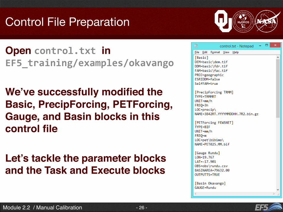
Open control.txt in EF5_training/examples/okavango
We’ve successfully modified the Basic, PrecipForcing, PETForcing, Gauge, and Basin blocks in this control file
Let’s tackle the parameter blocks and the Task and Execute blocks

Module 2.2 / Manual Calibration
CrestParamSet and KWParamSet
- 27 -
Let’s go ahead and keep the original Wang Chu parameters, since we’re going to be calibrating anyway
But change the name of CrestParamSet to Okavango And kwparamset to Okavango Change the value of gauge in both blocks to Rundu

Module 2.2 / Manual Calibration
Task Block
- 28 -
In the task block,• Change the name from
RunWangchu to RunOkavango • Change BASIN to Okavango • Change PARAM_SET and
ROUTING_PARAM_SET to Okavango
• Change TIMESTEP to 3h • Our TIME_BEGIN should be
200701010300 • Delete TIME_WARMEND • Set TIME_END to 200801010000
And change TASK to RunOkavango

Module 2.2 / Manual Calibration
Create a Batch File
- 29 -
Right-click in some blank space in your EF5_training/examples/okavango folder, and select “New” and “Text Document” Name it RunEF5.txt Open it and type ..\..\software\EF5.exe Pause

Module 2.2 / Manual Calibration
Create a Batch File
- 30 -
Using the “File” menu, go to “Save As…” and then in the “Save as type:” dropdown box select “All Files (*.*)”
Save it as RunEF5.bat Double-click RunEF5.bat

Module 2.2 / Manual Calibration
Visualize the Output
- 31 -
Load the model output into Microsoft Excel
This time, when you add a chart, you’ll need to use the “Select Data” button in the “Chart” and “Design” tabs of the Ribbon
Click “Hidden and Empty Cells” and select “Connect data points with line”

Module 2.2 / Manual Calibration
Visualize the Output
- 32 -
Then add “Legend Entries (Series)” one at a time, for discharge, observations, and precip
In each, the first cell of the column (like B1) should be the “Series name:” and cells B2:B2920, for example, should be the “Series values”
Set the “Horizontal (Category) Axis Labels” to A2:A2920 and then click “OK”

Module 2.2 / Manual Calibration
Visualize the Output
- 33 -
Select the “Precip” series near the bottom of your new chart, right-click, and select “Format Data Series”
Plot it on the “Secondary Axis”

Module 2.2 / Manual Calibration
Visualize the Output
- 34 -
Invert the order of the values on the precipitation axis and increase the maximum to some larger value (20 seems to work well) so the precipitation moves out of the way of the discharge and observations
Change the precipitation data series to a “Clustered Column” chart
Change the colors of the time series, if you wish, along with the date labels on the horizontal axis

Module 2.2 / Manual Calibration
Visualize the Output
- 35 -
Follow the instructions from Module 1.3 to determine the NSCE, CC, and bias of this hydrograph
IMPORTANT – only compare the observations without points of missing data (marked as “nan” in Excel)To do this, bring up “Find and Replace” by using CTRL+FFind “nan” and replace it with nothing Then click “Replace All”

Module 2.2 / Manual Calibration
Visualize the Output
- 36 -
Start with CC• Use CORREL and compare discharge (Column B, rows 2
to 2920) to observations (Column C, rows 2 to 2920)• You should get something around 0.70

Module 2.2 / Manual Calibration
Visualize the Output
- 37 -
Next try bias• Add all the simulation values together
• Use this formula: =SUMIF(C2:C2920,″<>″&″″,B2:B290)• Instead of ENTER, press CTRL+SHIFT+ENTER after you type it
• Add all the observed values together (84,753)• Subtract observed values from simulated values (195,695.5)• Divide by the sum of the observed values (2.309)• And multiply by 100 (231%)

Module 2.2 / Manual Calibration
Visualize the Output
- 38 -
Finally let’s look at NSCE• Take the average of Column C (232.2) and fill all of Column I with
this same value• Use SUMXMY2 with Column C as the first argument and Column B
as the second (402,406,803)• Now use SUMXMY2 with Column C as the first argument and
Column I as the second (14,231,524)• Divide the first SUMXMY2 by the second, and subtract from 1
(-27.28)

Module 2.2 / Manual Calibration
Calibration Strategy
- 39 -
What does this tell us?• Well, it’s no surprise the bias is very high (over 200%)
given how much of an overestimate the red line in our hydrograph is
• The NSCE is < 0 which means our model shows “no skill”• But the correlation coefficient isn’t terrible, which
indicates, in a very general sense, that the timing of the hydrograph is okay
Taking all this into account, parameters that affect the magnitude of the hydrograph (a.k.a the water balance or CREST parameters) are going to be important
• Let’s start there

Module 2.2 / Manual Calibration
Calibration Strategy
- 40 -
I want to reduce the values in my simulation• I know WM is a parameter that has some importance• It can range from 5 to 250• Let’s increase it so the soil holds more water and the
stream flow is reduced – try 200.0 mm in your control file• My bias decreased to 167% from its previous 231%• My NSCE “improved” to -15.0 from -27.3

Module 2.2 / Manual Calibration
Calibration Strategy
- 41 -
Play around with B• Change it from 13.204 to something smaller, like 0.5• Now check your bias – I got 57%, so we’re getting better!• My NSCE is now -3.15
Module 2.2 / Manual Calibration
Calibration Strategy
- 42 -
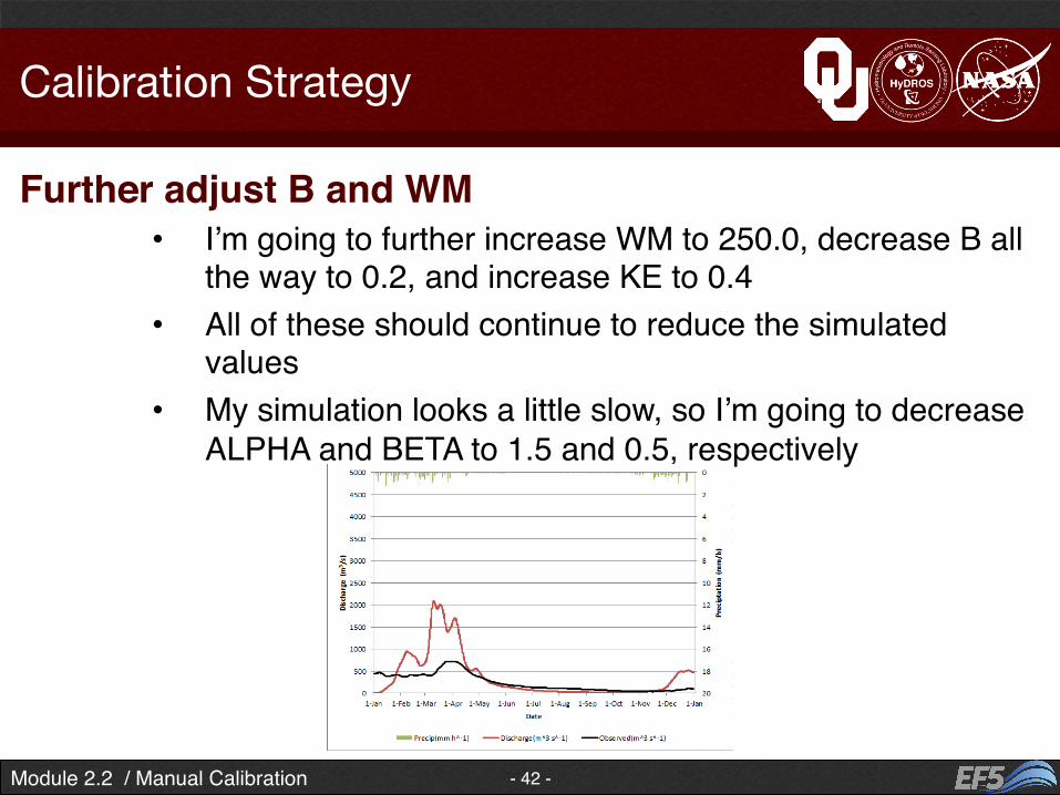
Further adjust B and WM• I’m going to further increase WM to 250.0, decrease B all
the way to 0.2, and increase KE to 0.4• All of these should continue to reduce the simulated
values• My simulation looks a little slow, so I’m going to decrease
ALPHA and BETA to 1.5 and 0.5, respectively

Module 2.2 / Manual Calibration
Calibration Strategy
- 43 -
We’re adjusting multiple parameters at a time just for fun, but a real strategy probably would take this more slowly and deliberately
• My bias is now -14%, so we got closer, but went too far• My correlation coefficient is 0.73, which suggests the timing
improved slightly from the original 0.70• My NSCE is now 0.01 – finally positive! This a great sign, but
we would have a long way to go still to get really good results

Module 2.2 / Manual Calibration
Calibration Strategy
- 44 -
Adjusting the vertical axis on our hydrograph to see things better…

Module 2.2 / Manual Calibration
Calibration Results
- 45 -
You start to see why a warm-up period is desirable
We now do a bad job of identifying the peak magnitude, though the timing seems generally okay
The lack of a warm-up period is also fairly obvious now, with the simulation results in the first half of January
In general, we respond too quickly (and too much) to precipitation and then drain it away too quickly at the end of the event – we need slower routing and more infiltration
Can you manually calibrate to a NSCE value of 0.10?

Module 2.2 / Manual Calibration
Calibration Results
- 46 -
Manual calibration can be useful to get us into the right neighborhood of parameters
We now have a much better idea of the general range of good parameters for this example
That makes automatic calibration an easier and better process!

Module 2.2 / Manual Calibration
Coming Up….
- 47 -
The next module is Automatic Calibration
You can find it in your \EF5_training\presentations directory
Module 2.2 ReferencesEF5 v0.2 Readme, (March 2015).EF5 Training Doc 2 – Hydrological Model Evaluation, (March 2015).EF5 Training Doc 4 – EF5 Control File, (March 2015).EF5 Training Doc 5 – EF5 Parameters, (March 2015).Guide for Estimating Ksat from Soil Properties, Section 618.88 of National Soil Survey Handbook, Natural Resources
Conservation Service, United States Department of Agriculture. Available online at http://www.nrcs.usda.gov/wps/portal/nrcs/detail//?cid=nrcs142p2_054224.


![04-Vortrag Wismar CIM [Kompatibilitätsmodus] - Fraunhofer IWU Chemnitz.pdf · © Fraunhofer IWU Prof. Neugebauer Dr. Bertram Schulz, Fraunhofer IWU Chemnitz, Präzisions- und Mikrofertigung](https://img.dokumen.tips/doc/110x75/5d4e0aff88c99324658bd8c4/04-vortrag-wismar-cim-kompatibilitaetsmodus-fraunhofer-iwu-chemnitzpdf.jpg)