Manila to Malaysia, Quezon to Qatar: InternationalMigration and its Effects on Origin-Country Human

Capital

Caroline Theoharides⇤

Amherst College

December 2016

Abstract

I estimate the effect of international migration on the human capital of children

in the migrants’ origin country. I use an original administrative dataset containing

all migrant departures from the Philippines and exploit variation across provinces in

destination-country demand for migrants. My estimates are at the local labor market

level, allowing for spillovers to non-migrant households. An average year-to-year

percent increase in migration causes a 3.5% increase in secondary school enrollment.

I use variation in gender-specific demand for migrants to show that effects are likely

driven by increased income rather than an increased expected wage premium for ed-

ucation.

JEL: F22, I25

⇤Department of Economics, AC #2201, Amherst College, Amherst, MA 01002. Email: ctheo-harides@amherst.edu. I thank the Overseas Worker Welfare Administration (OWWA), PhilippineOverseas Employment Administration (POEA), and Department of Education (DepEd) for ac-cess to the data and assistance compiling these databases. Chris Zbrozek provided invaluableassistance with constructing the BEIS dataset. I thank Kate Ambler, Manuela Angelucci, RajArunachalam, John Bound, Taryn Dinkelman, Susan Dynarski, Rob Garlick, Susan Godlonton,Jessica Goldberg, Joshua Hyman, Jessamyn Schaller, Jeffrey Smith, Isaac Sorkin, Rebecca Thorn-ton, and Dean Yang, as well as various seminar participants for valuable comments. I gratefullyacknowledge support from the Rackham Merit Fellowship and the National Science FoundationGraduate Research Fellowship.

International migration is a key labor market option for individuals from developing countries.

While international migration leads to increases in investment and consumption (Yang, 2008), one

concern about using migration as a tool for development is that it may reduce the stock of educated

labor in the origin economy, leading to brain drain (Gibson and McKenzie, 2011). An increase

in demand for migrants has the potential to alter the composition of the domestic labor force by

moving skilled workers abroad. Although much of the literature focuses on this loss of human

capital, it often misses the intergenerational response of children’s human capital in the country

of origin, which is an important component of whether a country experiences brain drain or brain

gain (Gibson and McKenzie, 2011).

In this paper, I causally estimate the effect of international migration on children’s human cap-

ital in the country of origin by exploiting shocks to demand for migrants. Most previous studies

only capture part of this effect by focusing on changes operating through a single channel, for

example migration-driven changes in income (Cox-Edwards and Ureta, 2003; Yang, 2008) or in

the wage premium for education (Batista, Lacuesta and Vicente, 2012; Chand and Clemens, 2008;

Shrestha, 2016). The handful of studies that attempt to estimate the overall effect generally rely

on identification strategies that compare migrant households to non-migrant households (Clemens

and Tiongson, 2013; Hanson and Woodruff, 2003; McKenzie and Rapoport, 2011) which will

understate the overall effects of migration, since non-migrant households also benefit from migra-

tion.

I conduct my analysis at the local labor market level, which allows me to capture effects of

migration on both migrant and non-migrant households, as well as through all potential chan-

nels through which migration could affect education. The importance of estimation at the local

labor market level can be highlighted by thinking about two key channels: the income channel

1

and the wage premium channel. First, increases in income due to remittances may ease liquid-

ity constraints and make higher levels of human capital investment possible. Many non-migrant

households, such as migrants’ friends and extended family, receive remittances (Yang and Choi,

2007), but even non-migrant households, such as local business owners, that do not receive re-

mittances likely benefit from increased spending of remittance dollars in the local economy as

well as from effects on domestic wages. Second, the expected wage premium for education may

change due to high wage opportunities abroad. Depending on the necessary level of education to

work abroad, the wage premium may increase or decrease, and the optimal level of educational

investment for children in both migrant and non-migrant households will change due to hopes of

obtaining high wage work abroad.

I identify the overall effect of migration on secondary school enrollment by exploiting spatial

variation across provinces in the Philippines in exposure to exogenous changes in destination-

country demand for Filipino migrants. Demand for migrants may change due to a variety of

factors outside the Philippines’ control, such as oil price shocks or changes in destination country

policy. Unlike bilateral migration channels like Mexico to the United States, Filipino migrants

work abroad in a wide variety of destination countries. Migrant networks are an important deter-

minant of where migrants locate and the occupations in which they are employed (Munshi, 2003).

As a result of these networks, when demand for migrants changes in a certain destination country,

this will have a larger effect on the migration rate in provinces specializing in sending migrants to

that destination.

I constructed an individual-level administrative dataset on all migrant departures from the

Philippines between 1992 and 2009. The data include both the province of origin and country

of destination for every migrant. Migration data rarely include both variables, and as a result of

2

their inclusion, I can create a plausibly exogenous instrument for the province-level migration

rate using variation generated by demand shocks to destination country-specific migrant networks

across local labor markets. Fluctuations in demand are determined outside the Philippines, and

any differences in network formation are controlled for with province fixed effects. As such,

the exclusion restriction should be valid, and these shocks should only affect education through

their effect on migration. Similar strategies are used in the labor literature to provide exogenous

variation in labor demand across local labor markets (Bartik, 1991; Blanchard and Katz, 1992;

Bound and Holzer, 2000; Katz and Murphy, 1992). In previous studies on migration, the historic

migration rate is often used to instrument for the contemporaneous migration rate using cross

sectional data (McKenzie and Rapoport, 2010; Woodruff and Zenteno, 2007). In such strategies,

endogeneity of the historic migration rate is a concern. My instrument combined with panel data

is a substantial improvement in causal identification.

I find that total secondary school enrollment increases by 3.5% in response to an average

year-to-year percent increase in province-level migration demand. The effects are largely driven

by increases in private school enrollment. Spillovers to non-migrant households appear non-

trivial, highlighting the value of estimating the effects of migration on education using a local

labor market approach.

I also provide suggestive evidence on whether the effects are driven by the income channel

or the wage premium channel by exploiting differences in gender-specific demand for migrants

across destinations. When demand increases for females, female enrollment may respond to

this change in their expected wage premium while male enrollment should not. Alternatively, if

income increases due to this migration, parents may choose to invest the same or different amounts

in male and female children, depending on sex preference and liquidity constraints. Thus, if male

3

and female enrollments respond equally to gender-specific migration demand, then the income

channel is likely dominant. If enrollment responds differentially, then the effects could be due to

either channel. I find similar increases in male and female enrollment, suggesting that the income

channel is dominant. One important caveat to this analysis is that it relies on the assumption that

households are able to accurately forecast wages by gender, which may not be the case.

This paper contributes to both the academic and policy literatures on migration. First, my

results add to the literature on the effects of migration on origin countries. My reduced form esti-

mates indicate an overall positive effect of labor migration on education, similar to the findings of

Dinkelman and Mariotti (2016) on the effects of low-skilled migration on educational attainment

in the African context. Much of the policy debate surrounding migration focuses on concerns

about changes in the composition of the domestic labor force due to the removal of skilled work-

ers. My results highlight that the removal of these skilled migrants increases the future stock of

high school educated labor in the Philippines, alleviating concerns of brain drain due to migration.

This is an important result for countries like the Philippines and Indonesia that export labor as a

development tool. Additionally, given that the effects appear to be driven by increases in income

from migration, ensuring direct, cost effective ways for migrants to remit money to their families

can lead to non-trivial increases in the human capital stock.

The remainder of the paper is organized as follows. Section 1 discusses background on migra-

tion and education in the Philippines. Section 2 presents a simple theoretical model of investment

in education in response to migration demand shocks. The data are presented in Section 3, fol-

lowed by the empirical strategy in Section 4. Section 5 discusses the main results, mechanisms,

and magnitudes of the estimates, and Section 6 concludes.

4

1 Background

1.1 Migration from the Philippines

The Philippine government created an overseas employment program in 1974 in response

to poor economic conditions in the Philippines. The program has grown dramatically; in 2011,

1.3 million Filipinos departed overseas on labor contracts (representing 2% of the working age

population). Contract migration is largely temporary and legal by way of licensed recruitment

agencies. Filipinos migrate to a wide range of destination countries (Table 1) and in a number of

occupations (Table 2). Saudi Arabia is the largest destination country, and the majority of migra-

tion is to the Middle East or Asia. Domestic helpers are the most common occupation. Based on

the perceived success of the migration program in the Philippines, several other countries, such

as Indonesia, India, and Bangladesh, have adopted or are in the process of adopting similar mi-

gration programs (Asis and Agunias, 2012; Rajan and Misha, 2007; Ray, Sinha and Chaudhuri,

2007; World Bank, 2011).

The rate of migration varies substantially across the Philippines. In 2009, the average mi-

gration rate across provinces for new labor contracts was 0.54% of the province population, and

varied from a maximum of 1.3% of the population in Bataan province to just 0.07% in Tawi-Tawi

province. This suggests that migration is a more important labor market option in certain parts

of the country than others. Figure 1 shows the migration rate in 1993 in each province. While

higher rates of migration are largely concentrated on the northern island of Luzon, there is sub-

stantial variation throughout the country. Even among high migration provinces, the occupation

and destination composition of migrants is heterogeneous due to specialization by provinces in

certain occupations and destinations. Figure 2 shows province-level migration rates in 1993 for

5

migrants to Hong Kong compared to Saudi Arabia. Migration to Hong Kong is concentrated in the

northern part of Luzon, whereas migration to Saudi Arabia is more heavily concentrated around

Manila and in Mindanao.

While migrant networks from Mexico to the United States were largely established due to

the location of railroads, there is not an obvious analogue in the case of Filipino migration. One

exception is religious composition. While the Philippines is a predominantly Catholic country,

parts of Mindanao are largely Muslim, and households in the Middle East often preferred migrants

of the same religion when hiring domestic helpers. Original hiring patterns based on religious

preference have led to large numbers of Filipinos from Mindanao migrating to the Middle East in

a variety of occupations. In general, however, Filipino migrant networks appear to be established

for largely idiosyncratic reasons, often due to the success of a handful of migrants from a province

to a destination. Migration from Batangas province to Italy illustrates this phenomenon, with a

single successful migrant in the 1980s leading to the majority of migrants to Italy originating from

Batangas today (Macaraig, 2011).

I exploit variation in destinations across provinces in order to identify the causal effect of

migration on secondary school enrollment. While no legal barriers prevent workers from other

provinces from acquiring these jobs, the reliance on social networks in choosing recruitment agen-

cies and obtaining jobs abroad creates rigidities across local labor markets.1

1.2 Migration and Education

To determine the sign of the wage premium effect in the Philippines, I examine the location of

Filipino migrants in the education distribution among all Filipino workers. I follow Chiquiar and

Hanson (2005) and plot the education distribution in Figure 3 of all migrants and non-migrants1In personal interviews with POEA staff, Barayuga (2013) states that migrants rely on family

members and friends who previously migrated to choose recruiting agencies and find jobs abroad.

6

using the 2000 Philippine Census.2 Panel A shows the distributions for all employed migrants and

non-migrants between the ages of 18 and 65. The share of migrants with less than a high school

education is smaller than the share of non-migrants with less than a high school education. The

opposite is true for high education levels. Panel A suggests that migrants from the Philippines

are positively selected. Similar figures by demographic subgroups such as age and gender also

imply that migrants are positively selected. While there is no required level of education for

contract laborers mandated by either the government or employers, employers appear to screen

on education, with few overseas options available for those individuals without at least a high

school education (Beam, 2013).

1.3 Education in the Philippines

To understand the margin along which individuals may alter their investment in schooling, I

note some key features of the Philippine education system. Primary education consists of six years

of schooling, and secondary education is four years, thus totaling ten years. Public primary educa-

tion is free and compulsory, whereas secondary education is free but not compulsory (Philippine

Republic Act 6655). Though secondary education is officially free, in addition to the opportunity

cost of schooling households must also cover the cost of miscellaneous fees, uniforms, school

supplies, transportation, food allowances, and textbooks (World Bank, 2001). Approximately fif-

teen percent of students drop out of secondary school,3 primarily to work or because the cost of

schooling is too high (Maligalig et al., 2010). Private education is a common alternative, and

eighteen percent of students enrolled in secondary school attend private school. The fees for pri-

vate school are substantially higher than for public school. While Filipinos perceive the quality2Minnesota Population Center (2014).3This is an underestimate as it only counts students who ever enrolled in secondary school.

8.5% of students drop out of primary school, and some never enter school at all (Maligalig et al.,2010).

7

of private school to be higher than public school and cite sending children to private school as a

major motivation for international migration (Bangko Sentral Ng Pilipinas, 2012), there is little

evidence to support the perception that the quality is higher (Yamauchi, 2005).

2 A Simple Theoretical ModelConsider a simple two-period model of investment in schooling developed by Becker and

Tomes (1986) and adapted by Acemoglu and Pischke (2001) to include credit constraints. In

period 1, the parent earns income y, consumes cp, saves s, and decides at the completion of

primary school whether to send their child to high school (e=1) or not (e=0). In period 2, the

child receives the expected skilled wage, ws, if the parents invested in a high school education

for the child, or the expected unskilled wage, wu, if the parent did not invest in education. I

assume that children with a high school education migrate abroad with probability p. Thus, ws =

pwa + (1 � p)wh, where wa is the wage abroad and wh is the skilled wage at home. Children

without a high school education can only work at home for wu. The cost of education is ✓, and I

assume no discounting. The utility of the household is defined as:

ln(cp) + ln(cc) (1)

where cc is the consumption of the child. I assume households are credit constrained, and

parents cannot borrow against a child’s future earnings to finance education. Therefore all direct

costs of secondary schooling must be paid from the household’s budget at the time of enrollment.

The parent maximizes equation (1) by choosing cp, cc, s, and e subject to the following constraints:

cp y � e✓ � s

cc wu + e(ws � wu) + s

s � 0

(2)

8

The first constraint is the household’s budget constraint, the second determines the child’s

consumption, and the third is the credit constraint. For wealthy families, credit market problems

are irrelevant, and educational investment will change only when the wage premium, ws � wu,

changes (Becker and Tomes, 1986; Acemoglu and Pischke, 2001). For poor families with income

y < wu, lifetime utility will be U(e = 1) = ln(y � ✓) + ln(ws) if the parents invest in schooling

versus U(e = 0) = ln(y) + lnwu if they do not. Comparing these two utility functions, parents

will only invest in education if:

✓ y

ws � wu

ws(3)

This implies the following:

1. As income, y, increases, investment in education increases.

2. As the high school wage premium, ws�wu, increases, investment in education increases.

Now consider a positive economic shock in a destination country that results in a persistent

increase in demand for migrants. As shown in Equation 3, this shock can affect a parent’s optimal

schooling choice for their child through two channels—a change in income or a change in the

high school wage premium.4 Such a shock may increase income, y, due to increased remittances.

Similarly, the shock may increase the wage premium by increasing the expectation of the skilled

wage, ws due to an increase in either the probability of migration, p or the overseas wage, wa.

Interpretation 1: A persistent increase in migration demand may affect investment in educa-

tion through both the income and wage premium channels.4There are other minor channels through which migration may affect parent’s optimal school-

ing investment not captured by this simple model. These include changes in household structure,intrahousehold resource allocation, marriage markets, demand for childcare, and children’s assis-tance with a family business. While this basic model does not focus on these channels, they areencompassed in my overall reduced form estimates of the effect of migration on enrollment.

9

To explore the relative importance of the income channel versus the expected wage premium

channel, I exploit differences in the destination and occupation patterns of male and female mi-

grants, as shown in Tables 1 and 2. Separate shocks to migration demand for male and female

migrants have implications for the theoretical framework. If there is no sex preference in terms of

educational investment, male and female enrollment should respond equivalently to any change

in income. However, if households are credit constrained or exhibit sex preference, enrollment

effects may differ by gender.

In terms of the wage premium channel, an increase in demand for migrants in predominantly

female occupations should only change the wage premium for females, given the gender-specific

nature of both foreign and domestic employment for Filipinos.5 Thus, female enrollment should

respond to increased demand, but male enrollment should not.

Interpretation 2: If male and female enrollments respond equally to gender-specific migration

demand, then it is likely that the income channel is dominant. If enrollment responds differentially,

this could be due to either channel or some combination.

There are two important caveats to this interpretation. First, households may not accurately

forecast wage information by gender. Households may assume that the increase in female wages

implies increases in wages for both genders, and accordingly, enrollment may respond equally for

men and women to the perceived increase in the wage premium. Second, if there is sex preference

such that parents would invest additional income in boys’ education but not girls’, an increase in

demand for female migrants could increase female enrollment through the wage premium channel

and male enrollment through the income channel. This could lead to equivalent increases in

enrollment even though both channels are present. While I cannot rule out this possibility, there

is little evidence of sex preference in the Philippines (Cruz and Vicerra, 2013).5See Online Appendix A for a discussion of the gender specificity of domestic employment.

10

One remaining point is how individuals form expectations of overseas wages. Delavande,

Gine and McKenzie (2011) and Jensen (2010) suggest that individuals in developing countries

form expectations using social networks and community outcomes. Thus, I assume individuals

form expectations about migration demand based on the outcomes they observe in their local

labor market.6 A number of papers in the U.S. examine how labor market expectations affect

the decision to enroll in post-secondary education. Much of the existing literature focuses on

either the effect of contemporaneous labor market conditions on enrollment (Card and Lemieux,

2001; Freeman, 1976) or the effect of ex post earnings on enrollment (Cunha and Heckman, 2007;

Willis and Rosen, 1979), while a new literature examines the effects of ex ante expected returns

to schooling on the enrollment decision (Attanasio and Kaufmann, 2010).

Since I do not have data on the perceived ex ante migration rate, I assume that parents form

expectations of migration demand based on the observed migration rate. Households will only

alter investment in education in response to changes in the expected wage premium if parents at

least partially observe the change in migration demand and perceive this change as permanent. In

Section 5.1, I use a Fourier frequency decomposition to show that changes in migration demand

are overwhelmingly low frequency, implying they are both predictable and persistent. Thus, it is

reasonable for parents to alter expectations of the wage premium based on the observed migration

rate.

3 DataI construct an original dataset of all new migrant departures from the Philippines between

1992 and 2009. The data are from the Philippine Overseas Employment Administration (POEA)

and the Overseas Worker Welfare Administration (OWWA). Both under the Department of Labor6I define the local labor market as the province because recruitment agencies are granted the

authority to recruit at the province level.

11

and Employment (DOLE), these agencies are responsible for overseeing various aspects of the

migration process. Prior to deployment, all contract migrants must visit POEA to have their

contracts approved and receive exit clearance. As a result, POEA maintains a rich database on all

new contract hires from the Philippines, encompassing 4.8 million individual-level observations

of migrant departures. The database includes the individual’s name, date of birth, sex, marital

status, occupation, destination country, employer, recruitment agency, salary, contract duration,

and date deployed.

OWWA is responsible for the welfare of overseas workers and their families, and all migrants

are required to become members of OWWA. OWWA maintains a membership database of new

hires and rehires similar to that housed at POEA with approximately 1 million observations per

year. Unlike the POEA data, home address of the migrant is included in the OWWA database.

Because OWWA membership requirements changed substantially over the sample period, I match

the OWWA data to the POEA data using fuzzy matching techniques (Winkler, 2004) in order to

obtain a consistent sample of new migrant hires. This adds home address to the POEA data,

creating a unique dataset including the origin and destination of all new contract migrants from

one of the world’s largest labor exporters. I then calculate province-level migration rates by

aggregating the number of migrant workers in each province-year and dividing by the working-

aged population in the province.

Data on public and private secondary school enrollment are from the Philippine Department

of Education (DepEd). Public school data are from the Basic Education Information System

(BEIS). Started in 2002, it includes school-level data on enrollment, number of dropouts, reten-

tion, number of teachers, and number of classrooms. I aggregate school-level data to calculate

province-level public school enrollment. Private school data are available at the division level.

12

Divisions are a geographic unit smaller than provinces, but larger than municipalities used for

the oversight of the education system. I aggregate divisions to calculate province-level private

school enrollment. To create overall province-level enrollment rates, I calculate total provincial

secondary enrollment from public and private counts, and divide enrollment by the population in

the province aged twelve to seventeen. See Appendix B for a more thorough discussion of both

the migration and education datasets and their construction.

Table 3 presents summary statistics over my sample period.7 The average provincial-level

migration rate is 0.42% and ranges from near zero to 1.59% of the population.8 I also calculate

gender-specific migration rates. Women migrate at a higher rate than men: 0.25% of working-

aged females migrate compared to 0.16% of men. The average province has a total secondary

school enrollment rate of approximately 57%. The range is large, with the lowest rate of enroll-

ment at 14% and the highest near 92%. Females are enrolled in both public and private school at

higher rates than males. About 46% of the school-aged population is enrolled in public schools,

while approximately 11% are enrolled in private schools.

4 Empirical StrategyThe basic specification identifying the effect of migration on enrollment is:

EnrollRatept = �0 + �1MigRatept�1 + ↵p + �t + ↵p ⇤ timet + ✏pt (4)

where EnrollRatept is the secondary school enrollment rate, defined as the percent of chil-

dren aged twelve to seventeen enrolled in high school in province p, year t.9 MigRatept�1 is the

7Because OWWA did not collect home address in all years of the sample, province-level mi-gration rates cannot be constructed in 1999-2003, limiting the sample to beginning in 2004.

8The 2% rate of migration stated earlier includes both new hires and rehires.9The results are robust to other definitions of the school-aged population. I follow the Depart-

13

province-specific migration rate in year t�1, defined as the percent of the total working age popu-

lation in province p, year t�1 who migrate.10 Province fixed effects, ↵p and year fixed effects, �t,

remove province-specific and year-specific unobservables respectively. Province-specific linear

time trends, ↵p ⇤ timet, remove province-specific unobservables that are trending linearly over

time. ✏pt is the error term and is clustered by province. The Philippines has 80 provinces and 4

districts of Manila, resulting in p equal to 84.

My identifying variation is within-province deviations in the outcome of interest from a linear

trend. The inclusion of province and year fixed effects as well as province-specific linear time

trends resolves some concerns of omitted variables bias. However, a number of threats to the

validity of the identification strategy remain. First, province-year specific omitted variables can

lead to bias. For instance, if a province had a large factory close in a given year, this could lead

to both an increase in the province-specific rate of migration abroad due to limited job opportu-

nities at home and to an increase in the high school enrollment rate as individuals stay in school

longer due to a lower opportunity cost. As a result, �1 would be biased upward. In addition to

possible omitted variables, reverse causation could also lead to upwardly biased point estimates.

Specifically, high enrollment rates in a given province may cause migration rates to increase.

4.1 Migration Demand Index

To address these threats to causal identification and isolate changes in migration demand from

changes in migration supply, I instrument for the migration rate using a migration demand index.

I create a Bartik-style instrument (Bartik, 1991; Blanchard and Katz, 1992; Bound and Holzer,

2000; Katz and Murphy, 1992) by exploiting destination country-specific historic migrant net-

ment of Education’s definitions and Maligalig et al. (2010) in my choice.10Because the school year commences in June, the annual migration rate that could be observed

to make enrollment decisions at time t is the migration rate at time t� 1.

14

works across provinces. Rather than predicting employment growth as is standard in this litera-

ture, I create an index of the predicted number of migrants in each province-year. To predict the

number of migrants, I weight the total number of migrants nationally to 32 distinct destinations

by the province share of the national total to that destination in a base period. I then sum over

all 32 destinations to predict the total number of migrants in each province-year.11 Specifically, I

define the migration demand index as follows:

Dpt =X

i

MitMpi0

Mi0(5)

where Dpt is the predicted number of migrants in province p, year t, Mit is the number of

migrants to destination i, year t in the Philippines as a whole, andMpi0

Mi0is the share of migrants at

baseline in province p, destination i, out of the total number of migrants nationally at baseline in

destination i. I define baseline as 1993.12 By using these baseline shares, I am implicitly assuming

that the distribution of migrants to a given destination is stable across the Philippines over time,

or at least a reasonable predictor of future distributions of migrants (Munshi, 2003; Woodruff and

Zenteno, 2007). If this is not the case, the instrument will be a poor predictor of the province-

specific migration rate. I then divide the index by the working population in the base year in order

to obtain a predicted migration rate.

Panel B of Table 3 shows summary statistics for the Bartik-style instrument. The constructed

total migration demand index exhibits similar patterns as the actual migration rate. The main11These 32 destinations represent 98% of migration episodes. The results are not sensitive to

the number of destinations used in the index. I also create two analogous indices that exploitoccupation-specific and occupation x destination country-specific historic migration networks.The results are robust to the choice of index, and are shown in Online Appendix Table 1.

12The first and second stage results are robust to using any year from 1993 to 1998 as the baseyear and are shown in Online Appendix Table 2.

15

difference is that the Bartik-style instrument has a much larger maximum value. This is because at

baseline (1993) the four districts of metro Manila composed a much larger share of total migration

than in later periods, since migration spread more evenly across the Philippines over time. Within-

province variation in the instrument is due to fluctuations in destination country demand. Online

Appendix C discusses in detail the factors driving changes in demand across destination countries,

namely oil prices, policy changes, and overall economic conditions.

I then estimate Equation (5) using the migration demand index to instrument for the actual

province-level migration rate. This is an improvement on the OLS fixed effects estimation strategy

for a number of reasons. First, it isolates the effects of changes in migration demand, rather than

confounding changes in demand with changes in supply. Returning to the example of the factory

closure, now if a factory closes in province p, year t, it will not affect the predicted migration rate

as long as the factory closure does not affect the total demand for overseas migrants. I argue in

Section 4.2 that demand is determined by destination countries. Thus, while this factory closure

may result in a shift in the allocation of migrants across provinces, it will not affect total overseas

migration. This potential shift in the allocation of migrants across provinces is one reason why

OLS estimates may be biased despite the fact that migration demand is determined outside the

Philippines. Further, it seems highly unlikely that a factory closure today affects shares at baseline.

The index alleviates concerns of any province-year specific omitted variables since they no longer

affect the constructed migration rate. Further, reverse causation is also no longer a concern unless

the high school enrollment rate in a province drives destination country demand at the national

level. Given that migrants are spread across the Philippines and that demand is from outside the

country, this seems unlikely.

My approach differs from the numerous papers that use the historic migration rate as an in-

16

strument for the contemporaneous migration rate (McKenzie and Rapoport (2010); Woodruff and

Zenteno (2007), among others) in two ways. First, I use the Bartik-style instrument while other

papers instrument for the migration rate with the historic migration rate, and second, I have a

panel data set whereas these papers generally use cross sectional data. A common critique of

the historic migration rate instrument is that the results may be biased since they cannot control

for unobserved province-specific variables in the cross sectional data. This raises the question of

whether it would be sufficient in my context to use the simpler historic migration rate as an instru-

ment in the panel data instead of the Bartik-style instrument, given that the panel data allows me

to control for province-specific unobservables. I show in Online Appendix D that the shift share

instrument has a strong first stage after the inclusion of the province fixed effects and linear time

trends, while the first stage is weak with the historic migration rate instrument when province

controls are added.

It is unsurprising that the shift share instrument is a better predictor of contemporaneous mi-

gration rates. While the historic migration rate assumes that provinces with high migration in the

past still have high migration today, the Bartik-style instrument accounts for destination-specific

changes in demand over time. Thus, my identification strategy improves upon the common his-

toric migration rate instrument by both controlling for unobserved province-specific variables and

by more accurately exploiting historic migration networks.

4.2 Identifying Assumptions

For this analysis to provide a causal estimate of the effect of migration demand on secondary

school enrollment, a number of identifying assumptions must hold. First, to satisfy the relevance

condition, there must be variation in the province-specific destination shares at baseline. If, for

instance, each province sent an equal share of migrants to Saudi Arabia in the base period, then the

17

instrument would explain little of the variation in province-level migration rates. Online Appendix

Table 3 shows that there is substantial variation in the size of the province shares to a given

destination country, thus satisfying this condition.

The second assumption, which is necessary for exogeneity, states that the total number of mi-

grants departing from the Philippines annually is determined by host country demand and there-

fore uncorrelated with province-level shocks. I argue that there is a large potential supply of

Filipinos who want to migrate, and the number hired is determined by demand from overseas em-

ployers. McKenzie, Theoharides and Yang (2014) suggest, based on evidence from 2010 Gallup

World Poll, that there may be as many as 26 million Filipinos who would like to migrate, com-

pared to only 2 million who currently work abroad each year. Further, they report from qualitative

interviews with recruiting agencies that there is an excess supply of Filipinos who want to work

abroad and that the overseas contract labor market is a buyer’s market.

If demand is determined outside the Philippines, then the total number of migrants in each

year should not be influenced by economic conditions in the Philippines, but rather by economic

conditions in destination countries. While cross regional variation in economic conditions within

the Philippines may shift the allocation of migrants across provinces, this will only affect the

strength of the first stage estimates rather than violating the identifying assumption since the

total number of migrants will remain the same. In Online Appendix E, I show that economic

conditions in the Philippines do not influence the total number of migrants, while allowing for

changes in the allocation of migrants across the Philippines due to differential internal shocks.

Finally, binding minimum wages for Filipino migrants, as found in McKenzie, Theoharides and

Yang (2014), indicate that an excess supply of laborers must exist at the minimum wage and the

quantity employed is determined by labor demand.

18

To further alleviate concern that the national flow of migrants is endogenous to differential

shocks to provinces over time, I also construct the migration demand index shown in equation

2 with Mit equal to the total number of migrants to destination i in year t net of province p’s

contribution to that total (Autor and Duggan, 2003). This approach is commonly referred to as

a “leave one out” or jackknife approach. As shown in Section 5.2, all results are robust to this

construction of the the index.

The final identifying assumption is that baseline shares are not correlated with trends in vari-

ables related to the outcome variable.13 For instance, one might worry that provinces that send

migrants to fast growing destinations have high growth in enrollment for reasons other than mi-

gration, leading to biased estimates. To alleviate this concern, I include province-specific linear

time trends in all preferred specifications. In Online Appendix E, I further test this exogeneity

assumption by comparing trends in education outcomes in high and low migration provinces. The

results of these tests in combination with the inclusion of province-specific linear time trends

reduce concerns of differential trending in the results.

4.3 Gender-Specific Demand Indices

In order to explore the mechanism through which migration affects human capital, I examine

the enrollment response to gender-specific demand for migrants as discussed in Section 2. Esti-

mating equation (4) with the province-level gender-specific migration rate as the key explanatory

variable will suffer from the same threats to identification as the overall migration rate. Thus, I

create gender-specific instruments:

Dgpt =X

i

MgitMgpi0

Mgi0(6)

13Province fixed effects absorb differences in levels of any province-specific omitted variables.

19

where Dgpt is the predicted number of migrants of gender g in province p, year t, Mgit is the

number of migrants of gender g to destination i, year t in the Philippines as a whole, andMgpi0

Mgi0is

the share of migrants at baseline of gender g in province p, destination i, out of the total number

of migrants nationally at baseline of gender g to destination i. The creation of this index does not

assume that the gender composition to different destinations is stable over time. Rather, it simply

assumes that, given a certain number of female migrants hired for a certain destination, the share

coming from each province is relatively stable over time. The identifying assumptions are the

same as discussed in Section 4.2, with an additional potentially omitted variable: the migration

rate of the opposite gender. I address this threat in Section 5.3

5 Results

5.1 Identifying Variation

One of the key assumptions in Section 2 is that changes in migration demand must be relatively

persistent in order for parents to change their expectations of a child’s future wages. Given that

children enter high school at age twelve, but cannot migrate until age eighteen, parents will only

change enrollment decisions due to the expectation that their child will migrate if they believe the

increased demand will persist for at least six years.

To formally test whether the variation in migration demand is high or low frequency, I filter

the migration demand index into high and low frequency components following Baker, Benjamin

and Stanger (1999) and Bound and Turner (2006). Low frequency variation suggests that changes

in migration demand are persistent over time, whereas high frequency variation would imply that

changes in migration demand are quite transitory. If demand is high frequency, it seems unlikely

that individuals will change their expectations of the wage premium in response to changes in

migration demand. If demand is instead low frequency, such labor market conditions are likely

20

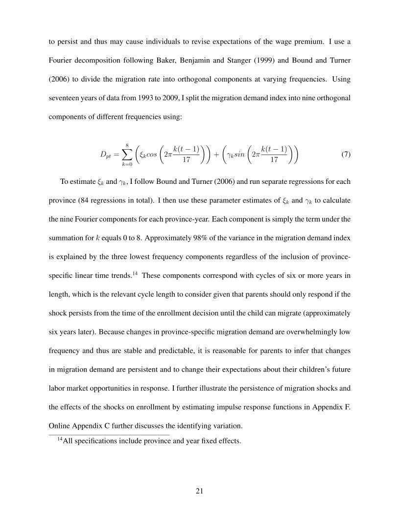
to persist and thus may cause individuals to revise expectations of the wage premium. I use a

Fourier decomposition following Baker, Benjamin and Stanger (1999) and Bound and Turner

(2006) to divide the migration rate into orthogonal components at varying frequencies. Using

seventeen years of data from 1993 to 2009, I split the migration demand index into nine orthogonal

components of different frequencies using:

Dpt =8X

k=0

✓⇠kcos

✓2⇡

k(t� 1)

17

◆◆+

✓�ksin

✓2⇡

k(t� 1)

17

◆◆(7)

To estimate ⇠k and �k, I follow Bound and Turner (2006) and run separate regressions for each

province (84 regressions in total). I then use these parameter estimates of ⇠k and �k to calculate

the nine Fourier components for each province-year. Each component is simply the term under the

summation for k equals 0 to 8. Approximately 98% of the variance in the migration demand index

is explained by the three lowest frequency components regardless of the inclusion of province-

specific linear time trends.14 These components correspond with cycles of six or more years in

length, which is the relevant cycle length to consider given that parents should only respond if the

shock persists from the time of the enrollment decision until the child can migrate (approximately

six years later). Because changes in province-specific migration demand are overwhelmingly low

frequency and thus are stable and predictable, it is reasonable for parents to infer that changes

in migration demand are persistent and to change their expectations about their children’s future

labor market opportunities in response. I further illustrate the persistence of migration shocks and

the effects of the shocks on enrollment by estimating impulse response functions in Appendix F.

Online Appendix C further discusses the identifying variation.14All specifications include province and year fixed effects.

21

5.2 The Effect of Migration Demand on Enrollment

In Table 4, Panel A, Column 1, I report the first stage results of the effect of the total migration

demand index on the total migration rate. The index has a positive and statistically significant

relationship with the endogenous variable, but the F-statistic is less than 10, indicating that weak

instruments are an issue (Stock and Yogo, 2002).15 In column 2, my preferred specification, I

add province-specific linear time trends to alleviate concerns about differential trending in omit-

ted variables across provinces. The F-statistic increases to greater than 10, and the relationship

between the endogenous variable and the instrument is larger in magnitude. The first stage point

estimate need not equal one since migrant networks are not perfectly predictive of migration rates

over time. In Column 3, I test the robustness of the results by dropping the highest migration

province, the 2nd district of Manila, to ensure that this is not driving the results.16 I further test

the robustness by weighting the regressions by the population at baseline (Column 4).17 In both

cases, the first stage appears robust. In the bottom row of Panel A, I report the p-value from the

Kleibergen-Paap underidentification LM test following Kleibergen and Paap (2006) and Baum,

Schaffer and Stillman (2007). In all cases, I reject the null that the structural equation is underi-

dentified at the 99% level.

Table 5, Panel A shows that total migration demand is positively related to secondary school

enrollment decisions. A one-percentage point increase in total migration demand causes school15When using robust standard errors, the Cragg-Donald Wald statistic is not valid. Instead, I

report the Kleibergen-Paap statistic (Kleibergen and Paap, 2006).16The first and second stage are robust to dropping each of the 84 provinces or simultaneously

dropping all districts of Manila.17I present unweighted results as my main specification for two reasons: 1) To estimate the

behavioral response of enrollment to migration demand shocks; and 2) To incorporate variationfrom both large and small provinces. The unweighted and weighted results, however, are qualita-tively similar as shown in Table 6. See Haider, Solon and Wooldridge (2025) for a discussion ofweighted versus unweighted results.

22

enrollment increases by 16.9 percentage points (Column 1). However, it is important to note that,

given average migration rates of 0.42% of the total province working population, a 1-percentage

point increase in the province-level migration rate is unrealistic. Instead, I calculate the average

year-to-year percentage point change in migration demand over the sample period to be 0.12 per-

centage points. For an average change in migration demand of 0.12 percentage points, enrollment

increases by 16.9*0.12=2.08 percentage points. This results in a 3.5% increase in enrollment. The

effects on female and male enrollment Panels B and C are similar to the overall results. Male and

female enrollment increase by 3.4% and 3.3% respectively, and I cannot reject that the coefficients

are the same.

In addition to the effect of migration demand on total secondary school enrollment, another

key consideration is whether households choose to send their children to public or private school.

One of the major motivations for international migration from the Philippines is the desire to

enroll children in private school (Asis, 2013). As income increases, parents may now choose

to switch to a type of schooling that they perceive as higher quality. The effect of the expected

wage premium on public and private enrollments remains an empirical question, and in Columns

2 and 3, I examine the response of public and private secondary school enrollment to changes

in total migration demand. Scaling the effects by the average year to year change in migration

demand, public school enrollment increases by 1.5% while private enrollment increases by 11.9%.

Given the average number of children enrolled in public and private school, this means almost

twice as many children enter private school. If I assume that most children who enroll in private

school in response to an increase in migration demand were previously enrolled in public school,

these results suggest that for every student switching to private school, there is another previously

unenrolled child who enrolls in public school. I examine the effects by grade level in Online

23

Appendix G.

Table 6 tests the robustness of the results. To address the identification concern of endogeneity

of the national totals to province-specific events, I conduct three tests. First, in Column 3, I drop

the province with the highest migration rate, the second district of Manila. Second, I drop the

highest migrant-sending provinces to each of the top three destinations.18,19 Third, I construct

the migration demand index by using the national total net of each province’s contribution to

that total. This approach is commonly referred to as a “leave one out” or “jackknife” version

of the Bartik instrument. The results are robust in all cases, indicating that the results are not

simply a reflection of the highest migrant-sending provinces nor endogeneity of the instrument

to differential province-level shocks. I further test the robustness of the results by replicating

Tables 4 through 7 in Appendix Tables 4 through 7 using the “leave one out” migration demand

index. In all cases, the results are robust, and I cannot reject the null hypothesis that the results are

the same when using the two constructions of the index, further alleviating concerns about large

migrant-sending origins driving the results.

In Column 2, I present the results without province-specific linear time trends. The results

are attenuated, imprecise, and have a weak first stage. I investigate this in Appendix Table 8, and

show that the weak first stage biases the results toward OLS, as discussed in Bound, Jaeger and

Baker (1995).20 Given the lack of strength of the instrument in this specification, I also construct

a weak instrument robust confidence interval for the Anderson-Rubin test of joint significance

of endogenous regressors (Anderson and Rubin, 1949; Baum, Schaffer and Stillman, 2007; Bazzi18Saudi Arabia, Japan, and Taiwan are the top three destinations, and Cavite, Bulacan, and

Pangisinan provinces are dropped respectively.19The results are also robust to dropping each of the 84 provinces, dropping the top three overall

migrant-sending provinces, or dropping all four districts of Manila.20In Column 6 of Appendix Table 8, I estimate a less restrictive model that includes province-

level baseline controls interacted with a time trend. Both the first and second stage results are moresimilar to the main results, though are still attenuated toward OLS given the weak first stage.

24

and Clemens, 2013). The 95% confidence interval is [-5.53, 25.77], which includes the main point

estimate of 16.976 (Column 1). In Columns 6, I include population weights. The weighted results

are attenuated slightly, but I cannot reject that they are the same as the main results.

5.3 Mechanisms

The results thus far provide evidence that total, public, and private secondary school enroll-

ment increase in response to increases in total migration demand. I next examine the effect of

gender-specific migration demand on school enrollment in order to provide suggestive evidence

on the underlying mechanisms. As discussed in Section 2, if the effects on male and female enroll-

ment are equal in response to an increase in female migration demand, then the income channel is

likely dominant. If the effects are not equal, either channel or some combination of the two could

be the dominant channel. Panels B and C in Table 4 show the first stage results for the male- and

female-specific migration demand indices. Both indices have a positive and statistically signifi-

cant relationship with the gender-specific migration rates. However, the male migration demand

instrument is weak. The higher standard errors in the male regressions compared to the female

regressions suggest that there is less variation in the male migration rate over the sample period.

To separate the mechanisms, however, I only need a shock in demand for either male or female

migration, and thus, I focus the gender-specific analysis on the effect of female migration demand.

Table 7 reports the effect of female migration demand on total, female, and male enrollment.

In Panel A, Column 1, a change in female migration demand has a positive and statistically signif-

icant effect on total secondary school enrollment. Specifically, an average year-to-year increase

in female migration demand of 0.05 percentage points leads to a 10.0*.05=0.5 percentage point

(0.9%) increase in secondary school enrollment.

While the same identifying assumptions must hold for the gender-specific demand indices as

25

for the total migration demand index, by splitting demand by gender I introduce another poten-

tially omitted variable: the migration rate of the opposite gender. Consider the effect of female

migration demand. If provinces that are more affected by changes in the national number of fe-

male migrants (ie., higher base share provinces) also experience an increase in the male migration

rate, and male migration also has an effect on school enrollment, then the results will be biased.

As a first step, I test the robustness of the results to controlling for the male migration rate in all

specifications in Table 7. The results are robust to the inclusion of this control (Column 2).

However, the male migration rate is likely also endogenous and including it as a control could

bias the estimates. To account for the endogeneity of both the male and female migration rates, I

instrument for both rates using two instruments: the female migration demand index and the male

migration demand index. The results of this two endogenous variable, two instrument setup are

also robust (Table 7, Column 3).21

Turning to Panel B, female migration demand has a positive and significant effect on female

secondary school enrollment of 0.9%. In Panel C, the effects of female migration demand on male

enrollment are slightly smaller (0.8%), but I cannot reject that they are the same as the female en-

rollment results. This leads me to conclude that income, rather than the expected wage premium,

is likely the dominant channel through which migration affects school enrollment, though this

conclusion is subject to the caveats discussed in Section 2.

I next examine the response of public and private enrollment to a change in female migration

demand. The effects of female migration demand on male and female public school enrollment are

essentially identical (Column 4). The effects on male private school enrollment are not precisely21Alternatively, I parametrically vary the coefficient on the male migration rate to test if the

effect of the female migration rate is robust. I vary the coefficient on the male migration rate from-22.1 to 22.1, the necessary coefficient if the 3.5% increase in enrollment (Table 5) is due to malemigration. The female migration coefficient ranges from 8.7 to 11.4, compared to the estimate of10.0 (Column 1), suggesting that endogeneity of the male rate does not lead to bias.

26

estimated, but the magnitude of the point estimates is similar across genders, and I cannot reject

that they are the same (Column 7). These public and private school results reinforce that the

income channel is likely dominant.

5.4 Interpreting Effect Sizes

The results suggest that an average year-to-year increase in total migration demand leads to a

3.5% increase in total secondary school enrollment. Given that the average province sends 2,458

migrants and has 80,789 students enrolled in secondary school, my main point estimate (Table

5) suggests that a 1 percentage point increase in migration demand off a mean migration rate of

0.42% would lead to a 238% increase in migration. Thus, given that the average province sends

2,458 migrants, this results in 5,852 new migrants. A 16.9 percentage point increase in total

secondary school enrollment off a sample mean of 56.9% enrolled results in a 29.7% increase in

enrollment. This results in 23,994 new students enrolled for every 5,852 new migrants. Every

additional migrant causes 4.1 more children to enroll in secondary school.

This is a substantial effect, but should be considered an upper bound. One important consid-

eration is that I only estimate the effect of new hire migration on secondary school enrollment. If

rehires are positively correlated with both new hire migration and enrollment, I will overstate the

results. McKenzie, Theoharides and Yang (2014) find that a 1% increase in GDP leads to a 2.6%

increase in new hires and a 1.9% increase in rehires. Based on their mean values, a 1% increase

in GDP results in 121 new hires and 148 rehires. Thus, for every 1 additional new hire, there are

approximately 1.2 additional rehires. This allows me to place bounds on my results. If rehires

and new hires affect secondary school enrollment equally, then each new migrant will result in 1.9

additional children enrolled versus 2.2 additional enrolled children from each rehire, for a total

of 4.1 children. However, new hires and rehires may not have equivalent effects on enrollment.

27

Liquidity constrained households may find the liquidity constraint loosened to increase education

in response to new migration, and so when the migrant is rehired, there is no enrollment response.

Thus, each new migrant likely induces between 1.9 and 4.1 children to enroll.

How do these effect sizes compare to previous estimates? Yang (2008) estimates the effect

of differences in exchange rate shocks faced by Filipino migrant households in light of the Asian

financial crisis on school enrollment, among other outcomes. Using data from the Philippine

Family Income and Expenditure Survey (FIES), he finds that a 10% improvement in the exchange

rate experienced by migrant households leads to a 6% increase in remittances and a 1% increase

in total school enrollment. A 6% increase in remittances is 2,171 pesos in Yang’s sample and,

for every 230,957 additional pesos remitted, one additional child is enrolled in school.22 Using

data from the 2006 FIES, I determine that the average remittance receiving household receives

76,273 pesos of remittances each year. I also use the 2006 FIES to determine that for every one

contract migrant, four households receive remittances from abroad. A rough back-of-the-envelope

calculation suggests that each additional migrant results in 305,092 pesos of remittances. By

Yang’s estimate, each additional migrant should cause 1.3 additional children to enroll in school

(305,092/230,957) compared to 1.9 to 4.1 children based on my estimates.23

In order to determine if 305,092 pesos of annual remittances is reasonable, I consider the

salaries earned by Filipino migrants. The micro data from POEA include the contracted wage for

each new migrant. Using these data, the average annual wages earned by a new hire during the

sample period are 349,368 pesos. This suggests that migrants remit 87% of their earnings. A new22Based on Yang’s point estimates, if 100 households receive 2,171 pesos, then 0.94 more

children will go to school. Thus, the total amount of remittances required to get an additionalchild to enroll in school is 230,957 pesos (217,100/0.94).

23Note that the 76,273 pesos reported in the FIES are likely an underestimate. Akee and Kapur(2012) find that remittance amounts reported in survey data are about half the actual value ofremittances received. If household remittances in Philippines are actually 152,546 pesos, then byYang’s estimate, each additional migrant would cause 2.6 additional children to enroll in school.

28

paper by Joseph, Nyarko and Wang (2015) uses rich data on salaries and remittances for contract

migrants in the UAE (a key destination for Filipinos) and finds that migrants remit between 60

and 85% of their salary. Because I calculate remittances from all migrants whereas annual wages

from POEA only include new migrants, 87% is almost certainly an upper bound on the fraction of

income remitted since wages increase over time. Thus, average annual migrant wages are likely

greater than 349,368 pesos, placing the fraction of salary remitted well within the range of Joseph,

Nyarko and Wang (2015), and suggesting that 305,092 pesos of remittances is reasonable.

While Yang’s effects are smaller, it is important to note that Yang’s paper examines the effects

of an increase in remittances on households that already have a migrant abroad (and thus are

likely already receiving remittances). For households sending a new migrant abroad, the increase

in income and the relaxation of the liquidity constraint from the initial receipt of remittances is

likely more pronounced than for households that have received remittances for some time. Further,

Yang only estimates the effect of remittances on migrant households, thus missing spillovers to

non-migrant households due to increased spending in the local economy. Given these reasons, it

is not surprising that this paper finds larger effects than Yang.

Conducting a similar calculation for private school enrollment, 14,749 students are enrolled

in private school in the average province. This suggests that for each additional migrant, 2.5

additional students enroll in private school. Considering the potential upward bias from rehires,

this leads to a range of 1.1 to 2.5 additional enrolled children. I turn to Clemens and Tiongson

(2013) to contextualize these results. Using a regression discontinuity design, they compare the

households of individuals just above and below the cutoff on a Korean proficiency exam required

for migration to Korea. They find that for each additional migrant, there are 0.41 more children

enrolled in private school. To compare this to my results, it is important to remember that this

29

estimate assumes that there are no effects of migration on non-migrant households. Given that

each migrant on average sends remittances to four households, if the effects of remittances are

equal across migrant and non-migrant households, then each migrant would induce 4*0.41=1.64

additional students to enroll in school. This falls well within the range of my estimates. My upper

bound of 2.5 can be explained by two factors. First, Clemens and Tiongson again miss potential

spillovers to non-remittance receiving households. Second, they acknowledge that their sample is

both wealthier and better educated than the overall Philippine population.

6 ConclusionThis study shows that international migration leads to increases in the human capital of chil-

dren in the migrant’s country of origin. For each new migrant that leaves the Philippines, multiple

additional children enroll in high school. Given the magnitude of the results, the human capi-

tal stock of high school educated labor in the Philippines will increase in response to migration.

These increases in human capital appear to be driven by increases in income, rather than increases

in the expected wage premium.

More broadly, my results indicate that policy discussions on brain drain that fail to consider the

overall effect of migration on human capital may reach misleading conclusions. While skilled la-

bor migration changes the composition of the domestic labor force, the intergenerational response

to labor migration leads to overall increases in the human capital stock of high school educated

labor. For developing countries that rely on exporting labor as a development strategy, my results

suggest that such labor market strategies, in addition to increasing consumption and investment

at home, actually act as a tool to increase future education levels. Further, ensuring cost effective

and reliable means of remitting money to family members is necessary for developing countries

to realize these substantial gains in human capital from migration.

30

ReferencesAbrigo, Michael R.M., and Inessa Love. forthcoming. “Estimation of Panel Vector Autoregres-

sion in Stata: a Package of Programs.” Stata Journal.Acemoglu, Daron, and Jorn S. Pischke. 2001. “Change in the Wage Structure, Family Income,

and Children’s Education.” European Economic Review, 45(4-6): 890–904.Akee, Randall, and Devesh Kapur. 2012. “Remittances and Rashomon.” Center for Global De-

velopment Working Paper.Anderson, T.W., and Herman Rubin. 1949. “Estimation of the Parameters of a Single Equation

in a Complete System of Stochastic Equations.” Annals of Mathematical Statistics, 20: 46–63.Asis, Marla. 2013. Personal Correspondence. Manila, Philippines:Scalabrini Migration Center.Asis, Marla, and Dovelyn Rannveig Agunias. 2012. “Strengthening Pre-Departure Orientation

Programmes in Indonesia, Nepal, and the Philippines.” Migration Policy Institute Issue in BriefNo. 5.

Attanasio, Orazio P., and Katja M. Kaufmann. 2010. “Educational Choices and SubjectiveExpectations of Returns: Evidence on Intra-Household Decision Making and Gender Differ-ences.” NBER Working Paper 15087.

Autor, David H., and Mark G. Duggan. 2003. “Distinguishing Income from Substitution Effectsin Disability Insurance.” American Economic Review, 97(2): 119–124.

Baker, Michael, Dwayne Benjamin, and Shuchita Stanger. 1999. “The Highs and Lows of theMinimum Wage Effect: A Time-Series Cross-Section Study of the Canadian Law.” Journal ofLabor Economics, 17(2): 318–350.

Bangko Sentral Ng Pilipinas. 2012. “Consumer Expectations Report.”Barayuga, Helen. 2013. Personal Correspondence. Manila, Philippines:Former Director, Philip-

pine Overseas Employment Administration.Bartik, Timothy J. 1991. Who Benefits from State and Local Economic Development Policies?

Kalamazoo, MI: W.E. Upjohn Institute.Batista, Catia, Aitor Lacuesta, and Pedro C. Vicente. 2012. “Testing the ’Brain Gain’ Hypoth-

esis: Micro Evidence from Cape Verde.” Journal of Development Economics, 97(1): 32–45.Baum, Christopher F., Mark E. Schaffer, and Steven Stillman. 2007. “Enhanced routines

for instrumental variables/generalized methods of moments estimation and testing.” The StataJournal, 7(4): 465–506.

Bazzi, Samuel, and Michael A. Clemens. 2013. “Blunt Instruments: Avoiding Common Pit-falls in Identifying the Causes of Economic Growth.” American Economic Journal: Macroeco-nomics, 5(2): 152–186.

Beam, Emily. 2013. “Perceived Returns and Job-Search Selection.” Working Paper.Becker, Gary, and Nigel Tomes. 1986. “Human Capital and the Rise and Fall of Families.”

Journal of Labor Economics, 4: S1–S39.Blanchard, Olivier, and Lawrence Katz. 1992. “Regional Evolutions.” Brookings Papers on

Economic Activity.Bound, John, and Harry Holzer. 2000. “Demand Shifts, Population Adjustments, and Labor

Market Outcomes during the 1980s.” Journal of Labor Economics, 18(1): 20–54.Bound, John, and Sarah Turner. 2006. “Cohort crowding: How resources affect collegiate at-

tainment.” Journal of Public Economics, 91: 877–899.Bound, John, David A. Jaeger, and Regina M. Baker. 1995. “Problems with Instrumental Vari-

ables Estimation When the Correlation Between the Instruments and the Endogenous Explana-tory Variable is Weak.” Journal of the American Statistical Association, 90(430): 443–450.

31

Card, David, and Thomas Lemieux. 2001. “Dropout and Enrollment Trends in the PostwarPeriod: What Went Wrong in the 1970s.” In Risky Behavior among Youths: An EconomicAnalysis. , ed. Jonathan Gruber, 439–482.

Chand, Satish, and Michael Clemens. 2008. “Skilled Emigration and Skill Creation: A quasi-experiment.” Center for Global Development Working Paper 152.

Chiquiar, Daniel, and Gordon Hanson. 2005. “International Migration, Self-Selection, and theDistribution of Wages: Evidence from Mexico and the United States.” Journal of PoliticalEconomy, 113(2): 239–281.

Clemens, Michael, and Erwin Tiongson. 2013. “Split Decisions: Family Finance When a PolicyDiscontinuity Allocates Overseas Work.” Center for Global Development Working Paper 324.

Cox-Edwards, Alejandra, and Manuelita Ureta. 2003. “International Migration, Remittances,and Schooling: Evidence from El Salvador.” Journal of Development Economics, 72(2): 429–461.

Cruz, Christian Joy P, and Paolo Miguel Vicerra. 2013. “Fertility Behavior, Desired Numberand Gender Composition of Children: the Philippine Case.” Working Paper.

Cunha, Flavio, and James Heckman. 2007. “The Evolution of Inequality, Heterogeneity, andUncertainty in Labor Earnings in the U.S. Economy.” NBER Working Paper 13526.

Delavande, Adeline, Xavier Gine, and David McKenzie. 2011. “Measuring Subjective Expecta-tions in Developing Countries: A Critical Review and New Evidence.” Journal of DevelopmentEconomics, 94: 151–163.

Dinkelman, Taryn, and Martine Mariotti. 2016. “What are the Long Run Effects of LaborMigration on Human Capital? Evidence from Malawi.” American Economic Journal: AppliedEconomics, Forthcoming.

Freeman, Richard. 1976. The Over-Educated American. New York: Academic Press.Gibson, John, and David McKenzie. 2011. “The Microeconomic Determinants of Emigration

and Return Migration of the Best and Brightest: Evidence from the Pacific.” Journal of Devel-opment Economics, 95(1): 18–29.

Haider, Steven, Gary Solon, and Jeffrey Wooldridge. 2025. “What are We Weighting For?”Journal of Human Resources, forthcoming.

Hanson, Gordon H., and Christopher Woodruff. 2003. “Emigration and Educational Attain-ment in Mexico.” University of California at San Diego Working Paper.

Jensen, Robert. 2010. “The (Perceived) Returns to Education and the Demand for Schooling.”Quarterly Journal of Economics, 125(2): 515–548.

Joseph, Thomas, Yaw Nyarko, and Sing-Yi Wang. 2015. “Asymmetric Information and Remit-tances: Evidence from Matched Administrative Data.” Working Paper.

Katz, Lawrence F., and Kevin M. Murphy. 1992. “Changes in Relative Wages, 1963-1987:Supply and Demand Factors.” The Quarterly Journal of Economics, 107(1): 35–78.

Kleibergen, Frank, and Richard Paap. 2006. “Generalized Reduced Rank Tests Using the Sin-gular Value Decomposition.” Journal of Econometrics, 133(1): 97–126.

Macaraig, Mynardo. 2011. “‘Little Italy’ Rises on Philippine Hillside.” Planet Philippines.Maligalig, Dalisay S., Rhona B. Caoli-Rodriguez, Arturo Martinez Jr., and Sining Cuevas.

2010. “Education Outcomes in the Philippines.” ADB Economics Working Paper Series 199.McKenzie, David, and Hillel Rapoport. 2010. “Self-Selection Patterns in Mexico-U.S. Migra-

tion: The Role of Migration Networks.” Review of Economics and Statistics, 92(4): 811–821.McKenzie, David, and Hillel Rapoport. 2011. “Can Migration Reduce Education Attainment?

Evidence from Mexico.” Journal of Population Economics, 24: 1331–1358.

32

McKenzie, David, Caroline Theoharides, and Dean Yang. 2014. “Distortions in the Interna-tional Migrant Labor Market: Evidence from Filipino Migration and Wage Responses to Des-tination Country Economic Shocks.” American Economic Journal: Applied Economics, 6: 49–75.

Minnesota Population Center. 2014. Integrated Public Use Microdata Series. Minneapolis: Uni-versity of Minnesota.

Munshi, Kaivan. 2003. “Networks in the Modern Economy: Mexican Migrants in the U.S. LaborMarket.” Quarterly Journal of Economics, 118(2): 549–599.

Neumann, Todd C., Price V. Fishback, and Shawn Kantor. 2010. “The Dynamics of ReliefSpending and the Private Urban Market During the New Deal.” The Journal of Economic His-tory, 70(1): 195–220.

Rajan, S. Irudaya, and U.S. Misha. 2007. “Managing Migration in the Philippines: Lessons forIndia.” Centre for Development Studies Working Paper 393.

Ray, Sougata, Anup Kumar Sinha, and Shekar Chaudhuri. 2007. “Making Bangladesh aLeading Manpower Exporter: Chasing a Dream of US $30 Billion Annual Migrant Remittancesby 2015.” Indian Institute of Management Working Paper.

Shrestha, Slesh A. 2016. “No Man Left Behind: Effects of Emigration Prospects on Educationaland Labor Outcomes of Non-migrants.” Economic Journal, Forthcoming.

Stock, James H., and Motohiro Yogo. 2002. “Testing for Weak Instruments in Linear IV Re-gression.” NBER Working Paper No. 284.

Theoharides, Caroline. 2015. “Banned from the Band: The Effect of Migration Barriers forOverseas Performing Artists on the Welfare of the Country of Origin.” Working Paper.

Willis, Robert J., and Sherwin Rosen. 1979. “Education and Self-Selection.” Journal of HumanResources, 87(5): S7–S36.

Winkler, William E. 2004. “Methods for Evaluating and Creating Data Quality.” InformationSystems, 29(7): 531–550.

Woodruff, Christopher, and Rene Zenteno. 2007. “Migration Networks and Microenterprisesin Mexico.” Journal of Development Economics, 82(2): 509–528.

World Bank. 2001. “Filipino Report Card on Pro-Poor Services.” Report No. 22181-PH.World Bank. 2011. “Improving Capacity for Migration Management in Europe and Cen-

tral Asia.” [Available at: http://wbi.worldbank.org/sske/case/improving-capacity-migration-management-europe-and-central-asia].

Yamauchi, Futoshi. 2005. “Why Do Schooling Returns Differ? Screening, Private Schools, andLabor Markets in the Philippines and Thailand.” Economic Development and Cultural Change,53(4): 959–981.

Yang, Dean. 2008. “International Migration, Remittances, and Household Investment: Evidencefrom Philippine Migrants’ Exchange Rate Shocks.” Economic Journal, 118(2): 591–630.

Yang, Dean, and HwaJung Choi. 2007. “Are Remittances Insurance? Evidence from RainfallShocks in the Philippines.” World Bank Economic Review, 21(2): 219–48.

33

Figure 1: 1993 Migration Rates by Province

Note: Migration rates are defined as the percent of the working population who migrate abroad.

34

Fig

ure

2:19

93D

esti

nat

ion-S

pec

ific

Mig

rati

onR

ates

byP

rovi

nce

Not

e:M

igra

tion

rate

sar

edefi

ned

asth

eper

cent

ofth

ew

orkin

gpop

ula

tion

who

mig

rate

abro

ad.

35

Fig

ure

3:D

istr

ibuti

onof

Educa

tion

0.0

5.1.15.2.2

5

% of Total

Non

e

Some

Primar

y

Primar

y G

rad

Some

HS

HS G

rad

Some

Train

ing

Train

ing

Gra

d

Some

Col

lege

Col

lege

Gra

d

Post G

rad

A.

Ove

rall

0.0

5.1.15.2.2

5

% of Total

Non

e

Some

Primar

y

Primar

y G

rad

Some

HS

HS G

rad

Some

Train

ing

Train

ing

Gra

d

Some

Col

lege

Col

lege

Gra

d

Post G

rad

B.

Hig

h M

ig.

Pro

vin

ces

0.0

5.1.15.2.2

5

% of Total

Non

e

Some

Primar

y

Primar

y G

rad

Some

HS

HS G

rad

Some

Train

ing

Train

ing

Gra

d

Some

Col

lege

Col

lege

Gra

d

Post G

rad

C.

Fe

ma

le

0.0

5.1.15.2.2

5

% of Total

Non

e

Some

Primar

y

Primar

y G

rad

Some

HS

HS G

rad

Some

Train

ing

Train

ing

Gra

d

Some

Col

lege

Col

lege

Gra

d

Post G

rad

D.

Ma

le

0.0

5.1.15.2.2

5

% of Total

Non

e

Some

Primar

y

Primar

y G

rad

Some

HS

HS G

rad

Some

Train

ing

Train

ing

Gra

d

Some

Col

lege

Col

lege

Gra

d

Post G

rad

E.

<=

35

Ye

ars

Old

0.0

5.1.15.2.2

5

% of Total

Non

e

Some

Primar

y

Primar

y G

rad

Some

HS

HS G

rad

Some

Train

ing

Train

ing

Gra

d

Some

Col

lege

Col

lege

Gra

d

Post G

rad

F.

>3

5 Y

ea

rs O

ld

Sourc

e: 2000 P

hili

ppin

e C

ensu

s

Sh

are

of

Mig

ran

tsS

ha

re o

f N

on−M

igra

nts

Not

e:E

ach

bar

repre

sents

the

per

cent

ofm

igra

nts

(non

-mig

rants

)w

ith

agi

ven

level

ofed

uca

tion

.Tra

inin

gre

fers

tote

chnic

alan

dvo

cation

aled

uca

tion

.

36

Table 1. Top 10 Destination Countries

Destination PercentAvg. New

Contracts per Year Destination Percent Destination Percent1. Saudi Arabia 33.10 78,860 Japan 22.64 Saudi Arabia 49.192. Japan 16.04 38,205 Saudi Arabia 16.81 Taiwan 11.403. Taiwan 14.53 34,621 Taiwan 14.06 UAE 7.604. UAE 10.12 24,121 Hong Kong 12.82 Qatar 7.495. Hong Kong 8.92 21,247 UAE 10.01 South Korea 2.436. Kuwait 4.97 11,848 Kuwait 5.78 Kuwait 2.427. Singapore 1.44 3,438 Qatar 2.88 Japan 1.698. South Korea 1.44 3,435 Malaysia 1.57 Libya 1.479. Malaysia 1.38 3,298 Singapore 1.47 Brunei 1.1710. Bahrain 1.34 3,190 Lebanon 1.38 Singapore 1.02

Overall Female Male

Source: POEA and author's calculations.

Notes: The sample period is from 1992 to 2009. Percents are defined as the total number of migrants from the Philippines to each destination divided by the total number of migrants from the Philippines over the sample period.

37

Number of Migrants

% of Total Migrants

% Female in Occupation

1. Domestic Helpers 1,139,053 23.97 97.462. Performing Artists 696,504 14.66 95.143. Production 328,486 6.91 43.994. Caregivers 238,408 5.02 96.075. Laborers 237,064 4.99 11.886. Medical Workers 214,832 4.52 81.257. Plumbers 197,508 4.16 0.358. Engineers 191,816 4.04 3.489. Cooks and Waiters 163,382 3.44 53.2410. Building Caretakers 140,199 2.95 72.1511. Electrical Workers 137,306 2.89 19.9712. Carpenters 131,314 2.76 0.4113. Machine Fitters 92,946 1.96 2.6914. Tailors and Sewers 87,185 1.83 83.1615. Other Service Workers 80,832 1.70 54.6116. Freight Handlers 74,995 1.58 3.6217. Clerical Workers 63,516 1.34 51.3218. Transport Equipment Operators 52,664 1.11 5.3919. Production Supervisors 43,434 0.91 5.1420. Machine-Tool Operators 39,609 0.83 5.87

4,751,936 60.66

Table 2. Top 20 Occupations for Overseas Contract Workers

Occupation

Total (All Occupations)

Notes: The sample period is from 1992 to 2009.Source: POEA and author's calcuations.

38

Mean SD Min Max Panel A. Actual Migration Rate (%)

Total Migration Rate 0.42 0.26 0.02 1.59Female Migration Rate 0.25 0.16 0.02 1.29Male Migration Rate 0.16 0.17 0.00 1.39

Panel B. Migration Demand Index (%)Total Migration Rate 0.67 0.65 0.02 3.62Female Migration Rate 0.41 0.39 0.02 2.68Male Migration Rate 0.24 0.36 0.00 1.99

Panel C. School Enrollment Rates (%)Total 56.90 10.04 14.35 92.23Total Female 59.92 9.88 16.17 92.12Total Male 54.06 10.53 12.50 92.34Total Public 45.53 8.45 12.53 79.61Female Public 48.09 8.64 13.69 78.29Male Public 43.16 8.62 11.34 80.81Total Private 11.37 6.50 0.00 47.95Female Private 11.83 6.67 0.00 47.91Male Private 10.90 6.35 0.00 47.99

Table 3. Summary Statistics

Notes: The unit of observation is the province-year (N=502). In order to account for the one-year lag of the migration variables in my analysis, the sample period in Panels A and B is 2004-2009, while the sample period in Panel C is 2005-2010. All values are expressed as percentages. The migration rates are defined as the number of migrants out of the working population. The enrollment rates are calculated using the population aged 12 and 17 as the denominator. Sources: Department of Education, POEA, OWWA, and author's calculations.

39

Lag 1 Migration Demand Index

Plus Province-Specific Time Trends

Without 2nd DistrictPlus Population

Weights

(1) (2) (3) (4)Panel A. Lag 1 Total Migration Rate 0.276** 0.444*** 0.435*** 0.654***

(0.123) (0.125) (0.132) (0.096)N 502 502 496 502F-Statistic 5.04 12.57 10.94 46.12KP Underidentification Test (p-value) 0.0026 0.0019 0.0032 0.0014

Panel B. Lag 1 Female Migration Rate 0.435*** 0.504*** 0.513*** 0.487***(0.072) (0.080) (0.086) (0.057)

N 502 502 496 502F-Statistic 36.54 39.71 39.71 73.64KP Underidentification Test (p-value) 0.0011 0.0029 0.005 0.0027

Panel C. Lag 1 Male Migration Rate 0.327** 0.337 0.395* 0.136(0.133) (0.205) (0.223) (0.137)

N 502 502 496 502F-Statistic 6.07 2.69 2.69 0.99KP Underidentification Test (p-value) 0.0327 0.0752 0.0679 0.1387

Table 4. First Stage Analysis: Effect of Instruments on Migration Demand

Notes: The sample period is from 2005 to 2010 (N=502) with 1993 used as the base year in the construction of the instrument. All regressions include province and year fixed effects. Robust standard errors clustered at the province level are in parentheses. The unit of observation is the province-year. Since the standard errors are clustered, the reported F-statistic is the Kleibergen-Papp statistic. The KP Underidentification test reports the p-value of the Kleibergen-Paap underidentification LM test. The female and male migration rates are instrumented for with the gender-specific versions of the indices. In Column 3, I drop the Second District of Manila, which is the province with the highest migration rate. In Column 4, I weight the results by the province level population at baseline. The migration rate and the migration demand index are lagged by 1 year. *** indicates significance at the 1% level. ** indicates significance at the 5% level * indicates significance at the 10% level. Sources: POEA, OWWA, and author's calculations.

40

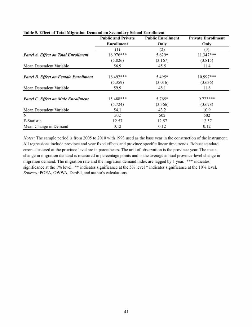
Public and Private Enrollment

Public Enrollment Only

Private Enrollment Only

(1) (2) (3)Panel A. Effect on Total Enrollment 16.976*** 5.629* 11.347***

(5.826) (3.167) (3.815)Mean Dependent Variable 56.9 45.5 11.4

Panel B. Effect on Female Enrollment 16.492*** 5.495* 10.997***(5.359) (3.016) (3.636)

Mean Dependent Variable 59.9 48.1 11.8

Panel C. Effect on Male Enrollment 15.488*** 5.765* 9.723***(5.724) (3.366) (3.678)

Mean Dependent Variable 54.1 43.2 10.9N 502 502 502F-Statistic 12.57 12.57 12.57Mean Change in Demand 0.12 0.12 0.12

Table 5. Effect of Total Migration Demand on Secondary School Enrollment

Notes: The sample period is from 2005 to 2010 with 1993 used as the base year in the construction of the instrument. All regressions include province and year fixed effects and province specific linear time trends. Robust standard errors clustered at the province level are in parentheses. The unit of observation is the province-year. The mean change in migration demand is measured in percentage points and is the average annual province-level change in migration demand. The migration rate and the migration demand index are lagged by 1 year. *** indicates significance at the 1% level. ** indicates significance at the 5% level * indicates significance at the 10% level. Sources: POEA, OWWA, DepEd, and author's calculations.

41

Main Results

Without Province-Specific Linear

Time TrendsWithout Highest

Migration Province

Without Highest Province to Top

Three Destinations

Instrument Constructed with

National Total Net of Province Contribution

Plus Population Weights

(1) (2) (3) (4) (5) (6)Panel A. Effect on Total Enrollment 16.976*** 6.091 18.606*** 15.930*** 19.890*** 10.324***

(5.826) (5.988) (6.369) (5.678) (7.193) (3.578)

Panel B. Effect on Female Enrollment 16.492*** 10.579 17.923*** 15.305*** 19.281*** 10.995***(5.359) (7.546) (5.831) (5.157) (6.621) (3.528)

Panel C. Effect on Male Enrollment 15.488*** -0.381 17.090*** 14.510*** 18.148*** 9.178**(5.724) (4.713) (6.234) (5.598) (7.033) (3.585)

N 502 502 496 484 502 502F-Statistic 12.57 5.04 10.94 11.89 9.68 46.12

Sources: POEA, OWWA, DepEd, and author's calculations.

Table 6. Robustness Checks for the Effect of Total Migration Demand on Secondary School Enrollment

Notes: The sample period is from 2005 to 2010 with 1993 used as the base year in the construction of the instrument. All regressions include province and year fixed effects and province specific linear time trends, except where indicated. Robust standard errors clustered at the province level are in parentheses. The unit of observation is the province-year. The mean change in migration demand is measured in percentage points and is the average annual province-level change in migration demand. The migration rate and the migration demand index are lagged by 1 year. *** indicates significance at the 1% level. ** indicates significance at the 5% level * indicates significance at the 10% level.

42

(1) (2) (3) (4) (5) (6) (7) (8) (9)Panel A. Effect on Total Enrollment 10.043** 10.227** 10.113** 2.937* 3.062** 3.137** 7.106** 7.165** 6.975*

(4.416) (4.410) (4.765) (1.549) (1.534) (1.525) (3.590) (3.618) (3.954)Mean Dependent Variable 56.9 56.9 56.9 45.5 45.5 45.5 11.4 11.4 11.4

Panel B. Effect on Female Enrollment 10.699** 10.937*** 10.854** 2.907* 3.062** 3.106** 7.792** 7.875** 7.748**(4.236) (4.211) (4.549) (1.501) (1.471) (1.466) (3.518) (3.539) (3.849)

Mean Dependent Variable 59.9 59.9 59.9 48.1 48.1 48.1 11.8 11.8 11.8

Panel C. Effect on Male Enrollment 8.516* 8.645** 8.550* 2.959* 3.055* 3.157* 5.557 5.590 5.393(4.378) (4.398) (4.760) (1.653) (1.653) (1.644) (3.479) (3.519) (3.861)

Mean Dependent Variable 54.1 54.1 54.1 43.2 43.2 43.2 10.9 10.9 10.9

N 502 502 502 502 502 502 502 502 502F-Statistic 39.71 39.55 29.59 39.71 39.55 29.59 39.71 39.55 29.59

Instrument for Female Mig. Rate Only Yes Yes No Yes Yes No Yes Yes NoInstrument for Both Male and Female Mig. Rate No No Yes No No Yes No No YesControl for Male Mig. Rate No Yes Yes No Yes Yes No Yes YesMean Change in Demand 0.05 0.05 0.05 0.05 0.05 0.05 0.05 0.05 0.05

Sources: POEA, OWWA, DepEd, and author's calculations.

Public and Private Enrollment Public Enrollment Only Private Enrollment OnlyTable 7. Effect of Female Migration Demand on Secondary School Enrollment by Gender

Notes: Columns 1, 4, and 7 are the basic specification and instrument for the female migration rate with the female migration demand index, Columns 2, 5, and 8 control for the male migration rate, and Columns 3, 6, and 9 instrument for both the male and female migration rate with the male and female migration demand indices. The sample period is from 2005 to 2010 with 1993 used as the base year in the construction of the instrument. All regressions include province and year fixed effects as well as province-specific linear time trends. Robust standard errors clustered at the province level are in parentheses. The unit of observation is the province-year. The mean change in migration demand is measured in percentage points and is the average annual province-level change in migration demand. The migration rate and the migration demand index are lagged by 1 year. *** indicates significance at the 1% level. ** indicates significance at the 5% level * indicates significance at the 10% level.

43

Manila to Malaysia, Quezon to Qatar: International Migration and its

Effects on Origin-Country Human Capital

Caroline Theoharides

Online Appendix

Online Appendix A: Gender Composition of Domestic JobsIn the simple theoretical model outlined in Section 2, I assume that an increase in demand

for migrants in predominantly female occupations should only change the wage premium for

females. This relies on the gender-specific nature of both foreign and domestic employment. One

concern might be that domestic jobs are not gender-specific in nature, and thus domestic wages

will rise for both male and female workers. This would lead to an increase the wage premium for

both genders. Using the 2007 Philippine LFS, I calculate that of the top 37 domestic occupations

(75% of all employment), 22 occupations are more than 75% male or female, 26 occupations

are more than 70% male or female, and only 4 occupations are between 40% and 60% male

or female. Online Appendix Table 9 shows these occupations and the percent female. Further,

using phil-jobs.net, the job posting website maintained by the Philippine government, of the 1,160

domestic job vacancies posted during the week of Sept. 9th, 2013, over 50% explicitly specified

the gender of the applicant. This suggests that domestic occupations are highly gender specific,

and a change in the supply of skilled female workers should increase wages for females more

than for males. Even if higher domestic wages increase the wage premium for both genders, the

increased probability of finding work abroad for females means the female wage premium will

increase by more.

44

Online Appendix B: Data ConstructionThis data appendix outlines the key technical details for the construction of both the migration

and education datasets used in this paper.

B.1: Migration Data

The migration dataset is constructed from the administrative databases of the Philippine Over-

seas Employment Administration (POEA) and the Overseas Worker Welfare Administration (OWWA).

POEA is tasked with approving migrant contracts and providing exit clearance. They maintain

a rich database on all new contract migrants, including data on name, date of birth, sex, marital

status, occupation, destination country, employer, recruitment agency, salary, contract duration,

and date deployed. OWWA is responsible for the welfare of overseas workers and their families,

and all migrants are required to become OWWA members. In order to check on the welfare of

migrant families, OWWA maintains a similar database to POEA, but also collects data on home

address of the migrant. OWWA membership requirements have changed substantially over the

sample period. Originally, OWWA required membership for all new hires, domestic helpers, and

seafarers, but since 2001, membership is required for all new hires and rehires.

In order to identify a consistent sample of new hires over the sample period, I combine the

two administrative datasets from POEA and OWWA using fuzzy matching techniques (Winkler,

2004). I match the data using first name, middle name, last name, date of birth, destination

country, gender, and year of departure. For the years of data used in this analysis, the overall

match rate is 94%. In 1993, the base year, the match rate is 90%. The match rates for 2005-2009

range from 96% to 98%, with a somewhat lower match rate of 80% in 2004.

While the match rates are high, one concern might be that match quality is differential by

45

migrant characteristics directly correlated with educational attainment. To test for this, I create

a binary variable equal to 1 if the match for a given migrant is successful and zero otherwise.

Using the individual-level migrant data, I then regress this binary variable on a number of migrant

characteristics. While ideally I would examine the effect of a migrant’s educational attainment on

match quality, education data are unfortunately not available in the migration data set. Instead,

I investigate demographic characteristics of the migrants, namely age and gender, since educa-

tional attainment likely varies by these demographics. I also examine the effect of migrant salary

and contract duration. The best proxy for educational attainment is salary since higher earning

migrants likely also have higher levels of education.

The results are shown in Appendix Table 10. In Column 1, I regress the match variable on

age, gender, contract duration, and salary. Given the sample size of over 1.6 million migrants, the

point estimates are unsurprisingly statistically significant. The magnitudes, however, are trivial.

The largest point estimate is for gender. With a mean match rate of 0.935, females are 0.001%

less likely to match between the two datasets. The main estimates in this paper also include

province and year effects as well as province-specific linear time trends. While I cannot include

the province fixed effects and trends in the test for match quality since the province variable is not

included in the POEA dataset, in Column 2 I add year fixed effects. The point estimates are again

extremely small. A $100 increase in wages, which represents over one-quarter of the total wage

given average wages in the sample of $417, would yield a 0.0004% decrease in the likelihood of

the match. With such small point estimates, it seems unlikely that any differences in match quality

by migrant characteristics have an effect on the results of the paper.

To calculate the number of migrants in each province, I aggregate the individual migrant

records from the matched dataset to the province level, which is my level of analysis, using

46

the home address variable. However, the home address variable includes municipality, but not

province. Out of 1630 municipalities, 332 have ambiguous names that are used in more than one

province or region. This accounts for between 10 and 19% of migration episodes depending on

the year. Thus, to calculate the number of migrants in the province, I assign municipalities with

repeated names their population share of the total number of migrants across municipalities with

the same name. The results are robust to other assignments.

Further, a share of migrants fail to report municipality in the OWWA database. I drop these

observations from the analysis. However, I test the robustness of the results to three different

methods of imputing municipality: 1) Based on municipality population shares; 2) Based on mu-

nicipality migration densities from the 2010 Philippine Census; and 3) By predicting the probabil-

ity of missing municipality based on observed migrant characteristics and assigning municipality

shares based on the mean predicted probability across migrants from that municipality. The results

are robust to the choice of missing municipality assignment.

To calculate the province-level migration rates, I divide the total number of migrant workers

in each province-year by the working aged population in the province. I define the working aged

population as 18 to 60 since 18 is the minimum age at which one can migrate. The age range 18

to 60 covers 99% of all migration episodes in my sample period. All population data are from the

1990, 1995, 2000, and 2007 Philippine Censuses from the National Statistics Office, and include

overseas contract workers. I linearly interpolate population counts for years between censuses.

One concern with the linearly interpolated values from the Census is that they may suffer

from multicollinearity with the province-specific linear time trends. To test for this, I include two

alternative specifications in Appendix Table 11. First, I estimate the effect of migration on school

enrollment using level values rather than rates. Specifically, I estimate the effect of the number

47

of migrants departing from the province on the total number of enrolled secondary students. The

instrument is constructed in the same way as described in Section 4, except that I no longer

divide by the working population at baseline. As a result, the instrument is just the predicted

number of migrants based on the base share. Second, I estimate the effect of the migration rate on

the secondary school enrollment rate using my standard instrument, but instead dividing by the

1993 working population and 1993 high school aged population to calculate the migration and

enrollment rates in order to avoid the linear interpolation.

In both cases, the results are robust to these alternative specifications. Column 2 presents the

level results. A one migrant increase in the number of migrants departing the province yields an

increase of 2.5 students enrolled. This falls well within the boundaries of my main results, which

suggest that for each migrant, 1.9 to 4.1 additional students are enrolled in secondary school. I

cannot reject the null hypothesis that my estimate of 2.5 students is equal to either 1.9 or 4.1.

Column 3 presents the results using the base year population in the construction of rates. These

results are more easily comparable to my main results (Column 1), and indicate that my results

are robust to this alternative specification.

B.2: Education Data

The education data used in this paper are from the Philippine Department of Education (DepEd).

The public school data are from the Basic Education Information System (BEIS), and include

school-level data on enrollment, dropout, retention, and a number of other variables. All public

schools are required to submit this data on an annual basis.

Private school data are available at the division level, which is a geographic unit larger than the

municipality, but smaller than the province. Private schools are not required to submit enrollment

data to DepEd, and so non-submission must be accounted for when calculating enrollment rates.

48

The private school data from 2002 to 2004 are the official figures from DepEd. For 2005 to

2010, I adjust division-level enrollment to account for non-submission. I calculate the submission

rate by dividing the number of schools that submitted by the total number of private schools in the

division. The median submission rate is 1, and the 5th percentile is 0.5, suggesting that compliance

is generally high. However, 47% of divisions do not have 100% compliance, suggesting that

adjustment is important. To adjust for compliance, I assume that complying and non-complying

schools are the same size. I then inflate enrollment by one divided by the submission rate. Further,

there are 120 observations (10%) between 2005 and 2010 that are missing or have unavailable

compliance rates. For these observations, I replace enrollment with the average enrollment for

the years immediately before and after. The results are robust to excluding missing values or non-

compliers. Neither official figures nor compliance rates are available for 2011 so I drop it from

my analysis.

After adjusting for compliance, I aggregate the public and private school enrollment data to

the division level. To calculate enrollment rates, I divide by the population in the province aged

twelve to seventeen, following DepEd’s definitions and Maligalig et al. (2010).

Online Appendix C: Identifying VariationOne critique of Bartik-style instruments is that the source of underlying variation is often un-

clear. To address this, in Online Appendix Figure 1 I plot total migration over time in each of the

9 destinations with the highest variances over the sample period in order to explicitly explore the

identifying variation.24 Migrant outflows change substantially over the sample period. Despite

fluctuations in certain destination-years, in general these plots of destination-specific migration

demand suggest that migration demand increased over time and that the variation in most desti-24Incidentally, these are also 7 of the top 10 largest destinations. Figures for all 32 destinations

are available upon request.

49

nations is fairly low frequency.

To further explore the determinants of demand, I uncover a number of institutional factors that

drive the identifying variation for the 9 highest variance destinations shown in Online Appendix

Figure 1. Panel A shows total migration to Saudi Arabia from 1992 to 2009. During the early part

of the sample period, migration fell due to the Gulf War. From 2003 onward, migration to Saudi

Arabia grew substantially as oil prices increased, and the hire of engineers, building caretakers,

domestic helpers, laborers, and medical workers increased substantially. The dip at the end of the

sample is due to a change in the minimum wage for domestic helpers imposed by the Philippines

in 2007 (McKenzie, Theoharides and Yang, 2014). With a minimum wage that was double the

previous rate ($400 per month from $200 per month), the number of domestic helpers fell from

12,550 in 2006 to 3,870 in 2007, though the hire of domestic helpers recovered by 2009.

Migrants to Japan are almost exclusively employed as Overseas Performing Artists (OPAs).

In Panel B, the large drop in the number of migrants to Japan in 2005 is due to barriers imposed

on migration of OPAs in response to pressure from the United States (Theoharides, 2015). The

dip in deployment of migrants to Japan between 1994 and 1995 was due to more stringent re-

quirements for OPAs imposed by the Philippine Labor Secretary in response to exploitation of

Filipinas (Philippine General Rule 120095).

Panels C, D, and F show steady increases in the number of Filipino migrants to the Middle East

from 2003 onward. This coincides with rising oil prices, and the number of migrants employed

as building caretakers, cooks, domestic helpers, engineers, plumbers, salesmen, and other service

workers increases substantially in these destinations during this period. Similar to Saudi Arabia,

the dip in the number of migrants in 2007 is due to the increase in minimum wage for domestic

helpers.

50

In Taiwan (Panel E), about 50% of migrants work in the production sector, which is largely

composed of factory workers. Growth in the hire of these workers over the sample period was

substantial due to growth in cell phones, computers, and other electronics during the 1990s, and

this growth remained steady through the 2000s. The other major occupations migrating to Taiwan

are caregivers and domestic helpers, though this declined substantially in 2006 for caregivers and

in 1997 for domestic helpers, likely due to the increased hire of these migrants from Indonesia.

The large drop in the number of workers to Taiwan in 2000 was due to a hiring ban on Filipino

workers imposed by Taiwan in June, 2000 due to deteriorating relations between Taiwan and the

Philippines.

Almost all migrants to Hong Kong (Panel G) are employed as domestic helpers. While there

are fluctuations in demand for these workers over the sample period, the general trajectory is

upward. Indeed, the number of domestic helpers increased from about 13,500 in 1992 to 25,000

in 2009. Migrants to Lebanon (Panel I) are also almost exclusively domestic helpers. The hire of

domestic helpers grew substantially starting in 1998 and by 2005, over 11,000 domestic helpers

were employed. However, in 2007, the Philippines imposed a two year ban on the deployment

of Filipinos due to fighting between Israel and Hezbollah. Finally, migration to Singapore (Panel

H) is mainly for domestic helpers, engineers, and medical workers. The growth at the end of the

sample period was due to a doubling of the hire of medical workers between 2007 and 2008.

To summarize, as discussed in 5.1 the majority of the variation in the migration demand index

is relatively low frequency, indicating that changes in migration demand are persistent. Policy

changes by destination countries and the Philippines, the price of oil, and growth in the electronics

field seem to be the drivers behind changes in the number of Filipinos migrating abroad each year

overall as well as to specific destinations.

51

Online Appendix D: Comparison of InstrumentsIn this appendix, I compare the Bartik-style instrument used in my main analysis with the

more commonly used historic migration rate instrument. As I discussed in Section 4.2, my iden-

tification strategy differs from the commonly used historic migration rate instrument by 1.) using

panel data instead of cross sectional data and 2.) using a Bartik-style instrument instead of the

historic migration rate instrument. In Appendix Table 12, I explore whether it would be suffi-

cient to simply use a historic migration rate instrument in panel data with province fixed effects

and province-specific linear time trends to resolve concerns about bias from province-specific

unobservables.

To create the historic migration rate instrument, I use the province-level migration rate 13

years prior to instrument for the current province-level migration rate in each of my sample years.

Columns 1 and 2 of Appendix Table 12 show the results using the historic migration rate instru-

ment. While there is a strong first stage in Column 1, when province and year fixed effects and

province-specific linear time trends are included in Column 2, the first stage results are weak, and

the first stage point estimate has the opposite sign of what is expected. If I instead instrument

with the Bartik-style instrument (Columns 3 and 4), the results are robust to the inclusion of the

fixed effects and linear time trends. The Bartik-style instrument does a better job of exploiting

the variation in migrant networks by predicting migration rates based destination-specific shifts

in demand rather than simply assuming that high migration provinces are always high migration

provinces. Thus, the combination of panel data and the Bartik-style instrument is an improvement

on previously used identification strategies in the migration literature.

52

Online Appendix E: Identifying AssumptionsIn Section 4.2, I discuss the identifying assumptions necessary for my analysis to provide a

causal estimate. In this appendix, I provide additional checks of two of the identifying assump-

tions. First, I provide additional evidence that the total number of migrants departing from the

Philippines is determined by host country demand. To further show that economic conditions in

the Philippines do not influence the total number of migrants, I regress the log number of mi-

grants in each of the 32 destination countries on log Philippine GDP, controlling for log GDP in

the top ten destinations for Filipinos. If economic conditions in the Philippines do not affect the

number of overseas workers, then Philippine GDP should not have an effect on migrant outflows.

Online Appendix Table 13 shows the results of this analysis. Out of the 32 destinations, Philip-

pine GDP only has a statistically significant effect in 2 cases, roughly what would be expected

due to chance. While the coefficients are not precisely estimated zeros, they are smaller and less

precisely estimated than the point estimates on log GDP in the top ten destinations.

Second, I conduct two additional checks to show that baseline shares are not correlated with

trends in variables related to the outcome variable. One way to test the validity of this exogene-

ity assumption is to compare provinces with low destination-specific baseline migration rates to

those with high rates and compare their trends in variables related to education. If, for exam-

ple, provinces with high baseline rates have higher growth in enrollment than provinces with low

baseline rates, I would incorrectly estimate that an increase in demand has a positive effect on

enrollment, when in actuality the increase in enrollment was at least partly due to differing trends.

Ideally I would compare trends in education outcomes prior to the start of the overseas mi-

gration program in areas that have high or low destination-specific migration rates at baseline.

However, the overseas migration program commenced in 1974, long before data on education

53

outcomes in the Philippines were available. In Online Appendix Figure 1, I plot the migration

outflows for the 9 destinations with the highest variation over the sample period. Migration for at

least some of the destinations remained relatively flat between 1993 and 2000, suggesting that the

importance of shocks to migration demand was much larger during the later years of the sample.

Thus, in provinces with high and low destination-specific migration rates, I examine trends in the

secondary school enrollment rate in the period from 1993 to 2000.25

In Online Appendix Figure 2, I plot the average province-level high school enrollment rates

for high and low migration provinces for each of the 9 destinations with the highest variation

in migrant counts.26 This allows for a visual evaluation of the parallel trends assumption: in

the absence of the change in migration demand, enrollment should have remained parallel. In

the pre-period, the trends in enrollment appear quite parallel. This suggests, for example, that

recruiters did not choose to locate in areas where education was increasing at a higher rate. In the

post period, enrollment in the low migration provinces appears to be catching up, perhaps due to

poverty reduction policies or policies geared at increasing educational attainment specifically.27

While this is concerning for the parallel trends assumption, it will lead to downward bias of the

estimates of the effect of migration demand on enrollment. Since I hypothesize that migration

demand increases enrollment, increases in education for low migration areas compared to high

migration areas will bias the estimates against finding an effect from increased migration demand.

To more rigorously examine if there are differential trends in enrollment, I estimate the fol-

lowing equation separately for each destination country in the pre period, post period, and full25I use destination-specific rates of migration at baseline to measure the level of treatment. The

baseline shares used in the construction of the index do not take into account the population of theprovince, thus they are not measuring the density of migration experienced by the province.

26Since DepEd did not release enrollment data prior to 2002, I use the LFS to calculateprovince-level high school enrollment rates.

27Total high school enrollment data are not available from 2001 to 2005.

54

sample:

�EnrollRatept = �0 + �1MigRatep0 + �t + ✏pt (8)

where �EnrollRatept is the percent change in the province-level high school enrollment rate

from time t � 1 to time t, MigRatep0 is the province migration rate at baseline, �t are year

fixed effects, and ✏pt is the error term. t is equal to 1993 to 2000 for the pre period and 2006

to 2011 for the post period. A non-zero value for �1 would lead to concern that the enrollment

rate is trending differentially for different levels of the migration rate. Online Appendix Table

14 shows the results. While the point estimates are not precise, there is substantial variation in

the magnitudes of the coefficients. However, many of the destinations with large point estimates

are small and account for little of the variation in migrant demand over the sample period. I

highlight the 9 highest variation destination countries in grey. Other than Lebanon and Singapore,

the coefficients in the pre-period for these highest variance destinations are close to zero. Given

that most of the identifying variation will come from changes in demand in these destinations, this

reduces concerns about differential trending driving the results. The inclusion of province-specific

linear time trends in all preferred specifications further alleviates this concern.

Online Appendix F: Impulse Response FunctionsIn order to further explore the effect of shocks to migration on enrollment over time, I estimate

a panel vector autoregression (VAR) to produce impulse response functions. Impulse response

functions best highlight the dynamic relationships estimated in the panel VAR. To do this, I use

Stata code written by Abrigo and Love (forthcoming) and follow the same procedure as Neumann,

Fishback and Kantor (2010). I select a lag structure of one year, which minimizes both the Akaike

55

Information Criterion (AIC) and the Bayesian Information Criterion (BIC). The AIC and BIC

reward goodness of fit of the model, while penalizing model complexity.

Appendix Figure 3 illustrates the responses of the migration rate and enrollment rate to a one

standard deviation shock in year zero. The solid line illustrates the impulse response function,

and the 90% confidence interval is outlined by dotted lines. The standard errors are clustered

by province, and calculated based on 1,000 Monte Carlo simulations. The X-axis is measured in

years, and the Y-axis is the percent deviation of the dependent variable from its mean in each year.

Enrollment increased in response to a shock in migration, though the increase did not occur

immediately (column 1, row 2), which is consistent with both the theoretical and empirical results

of the main paper. One year after the shock, enrollment increased by 0.5 percentage points, a

smaller effect than I find in my main results, which also include fixed effects and time trends. The

effects on enrollment appear to persist beyond one year. Six years after the shock, enrollment

is still slightly higher than before the shock, though the effect on enrollment is not statistically

different from zero beyond two years after the shock. It is also interesting to consider how much

enrollment increased in total for the six years following the shock. This can be determined by

aggregating the cumulative deviations, which are the area between the IRF line and the zero line.

The impulse response functions also provide further useful information on the persistence of

migration shocks. For a one standard deviation shock to migration, migration persists at a higher

rate than in the absence of the shock through six years after the shock, though after four years

the effect is not statistically different from zero. This corroborates the results from the Fourier

decomposition shown in Section 5.1, and provides further evidence that shocks to migration are

persistent and thus parents may anticipate that such migration opportunities will still exist when

their child is old enough to migrate.

56

Online Appendix G: Heterogeneity by Grade LevelSecondary school enrollment increases in response to increased migration demand due to

changes in income. However, given that the enrollment choice is sequential, aggregate enroll-

ment results may miss potentially interesting dynamics regarding the marginal student affected

by changes in migration demand. To examine these dynamics, I look at the effect of both total

and female migration demand on grade-level enrollment rates for each grade of high school. The

results are shown in Online Appendix Table 15.

Panel A shows the effects of total migration demand by grade level. An increase in migra-

tion demand causes an increase in enrollment across all grades, indicating marginal students are

induced into enrollment at all grade levels. However, the effects are largest in the 1st and 4th

year (5% and 4.3% respectively). For the first year, this is likely due to the bunching of dropouts

prior to the first year of high school. For 4th year students, liquidity constrained households may

choice to invest scarce resources in the student who will obtain a degree. This could be a result of

limited benefits to partial completion of high school. Thus, while there are marginal students in

all grades, this suggests a large number of students never enroll in high school either because of

liquidity constraints or the returns on the education investment are too low.

Panel B shows the enrollment response to female migration demand. The effects are positive

and quite similar across grade levels. Turning to Panels C and D, while there are equivalent effects

on male and female aggregate enrollment in response to a change in female migration demand,

there are heterogeneous effects when comparing the male and female enrollment responses by

grade level. While I cannot reject that the effects on male and female enrollment are equal (again

suggesting that the income channel is dominant), the differences in point estimates suggest that

some combination of the two channels may matter.

57

Appen

dix

Fig

ure

I:Tot

alM

igra

nts

inH

ighes

tV

aria

nce

Des

tinat

ions

040

00080

000

1200

00

# of Migrants

1990

1995

2000

2005

2010

Year

A. S

audi

Ara

bia

020

00040

00060

00080

000

# of Migrants

1990

1995

2000

2005

2010

Year

B. J

apan

020

00040

00060

00080

000

# of Migrants

1990

1995

2000

2005

2010

Year

C. U

AE

020

00040

00060

000

# of Migrants

1990

1995

2000

2005

2010

Year

D. Q

atar

020

00040

00060

000

# of Migrants19

9019

9520

0020

0520

10Ye

ar

E. T

aiwa

n

020

00040

00060

000

# of Migrants

1990

1995

2000

2005

2010

Year

F. K

uwai

t

020

00040

00060

000

# of Migrants

1990

1995

2000

2005

2010

Year

G. H

ong

Kong

020

00040

00060

000

# of Migrants

1990

1995

2000

2005

2010

Year

H. S

inga

pore

020

00040

00060

000

# of Migrants

1990

1995

2000

2005

2010

Year

I. Le

bano

n

Sour

ce: P

OEA

.

58

Appen

dix

Fig

ure

II:Par

alle

lTre

nds

Tes

tA

cros

sH

igh

and

Low

Bas

elin

eM

igra

tion

Pro

vince

s

.75.8.85.9Avg. HS Enroll. Rate

1995

2000

2005

2010

Year

A. S

audi

Ara

bia

.75.8.85.9Avg. HS Enroll. Rate

1995

2000

2005

2010

Year

B. J

apan

.75.8.85.9Avg. HS Enroll. Rate

1995

2000

2005

2010

Year

C. U

AE

.75.8.85.9Avg. HS Enroll. Rate

1995

2000

2005

2010

Year

D. Q

atar

.75.8.85.9Avg. HS Enroll. Rate

1995

2000

2005

2010

Year

E. T

aiwa

n

.75.8.85.9Avg. HS Enroll. Rate

1995

2000

2005

2010

Year

F. K

uwai

t

.75.8.85.9Avg. HS Enroll. Rate

1995

2000

2005

2010

Year

G. H

ong

Kong

.75.8.85.9Avg. HS Enroll. Rate

1995

2000

2005

2010

Year

H. S

inga

pore

.75.8.85.9Avg. HS Enroll. Rate

1995

2000

2005

2010

Year

I. Le

bano

n

Sour

ce: P

OEA

, OW

WA,

LFS

.

1st Q

uarti

le4t

h Q

uarti

le

59

Appen

dix

Fig

ure

III:

Impuls

eR

espon

ses

toa

One

Sta

ndar

dD

evia

tion

Pos

itiv

eShoc

kat

Tim

eZer

o

-1012 -.50.51

-.1-.050

.05

-.050

.05.1

02

46

02

46

Res

pons

e of

Enr

ollm

ent t

o Sh

ock

in E

nrol

lmen

t

Res

pons

e of

Enr

ollm

ent t

o Sh

ock

in M

igra

tion

Res

pons

e of

Mig

ratio

n to

Sho

ck in

Enr

ollm

ent

Res

onse

of M

igra

tion

to S

hock

in M

igra

tion

Percent Deviation from Mean

Year

s af

ter s

hock

60

Destination Occupation Occupation x Destination(1) (2) (3)

Panel A. Total Migration Demand Index 16.976*** 5.844 4.861(5.826) (4.803) (3.264)

N 502 502 502F-Statistic 12.57 21.62 37.39

Panel B. Female Migration Demand Index 10.043** 11.608*** 10.244***(4.416) (3.104) (3.505)

N 502 502 502F-Statistic 39.71 44.70 98.16

Index TypeAppendix Table 1. Effect of Total and Female Migration Demand on Total Secondary Enrollment, by Index Type

Notes: The sample period is from 2005 to 2010 with 1993 used as the base year in the construction of the instrument. Column 1 uses the destination-based index which is used for the main analysis. Column 2 creates the index in the same manner, but instead of destinations, it uses 38 occupation categories. Column 3 uses 38 x 32 occupation-destination groups to create the instrument. All regressions include province and year fixed effects as well as province-specific linear time trends. Robust standard errors clustered at the province level are in parentheses. The unit of observation is the province-year. *** indicates significance at the 1% level. ** indicates significance at the 5% level * indicates significance at the 10% level. Sources: POEA, OWWA, DepEd, and author's calculations.

61

1993 1994 1995 1996 1997 1998First stage 0.444*** 0.314*** 0.635*** 0.597*** 0.427* 0.903***

(0.125) (0.112) (0.123) (0.146) (0.238) (0.136)Second Stage 16.976*** 11.667* 9.360*** 8.705** 10.170** 6.753**

(5.826) (6.924) (3.534) (4.088) (4.817) (3.271)F-statistic 12.57 7.80 26.49 16.70 3.23 44.06

1993 1994 1995 1996 1997 1998First stage 0.504*** 0.361*** 0.568*** 0.598*** 0.444*** 0.671***

(0.080) (0.065) (0.056) (0.099) (0.137) (0.105)Second Stage 10.043** 1.972 10.258** 9.503** 12.492** 8.907**

(4.416) (2.714) (4.453) (4.495) (5.743) (3.472)F-statistic 39.71 30.60 100.99 36.34 10.58 40.60

Sources: POEA, OWWA, DepEd, and author's calculations.

Notes: The sample period is from 2005 to 2010 with the base year used in the construction of the index indicated in the the top row of the table. Panel A examines the effect of total migration demand on secondary school enrollment, while Panel B examines the effect of female migration demand on secondary enrollment. The results shown in the first column (base year 1993) are equivalent to the main results shown in the paper. All regressions include province and year fixed effects as well as province-specific linear time trends. Robust standard errors clustered at the province level are in parentheses. The unit of observation is the province-year. *** indicates significance at the 1% level. ** indicates significance at the 5% level * indicates significance at the 10% level.

Appendix Table 2. First and Second Stage Results with Alternative Base YearsPanel A. Effect of Migration Demand on Total Enrollment (Instrument: Migration Demand Index)

Base Year

Panel B. Effect of Female Migration Demand on Total Enrollment (Instrument: Female Migration Index)Base Year

62

25th 50th 75th SD Min MaxAlgeria 0.00 0.00 0.00 3.47 0.00 17.39Angola 0.00 0.00 0.00 3.03 0.00 14.00Australia 0.00 0.00 0.00 7.18 0.00 60.00Bahrain 0.14 0.26 1.30 2.10 0.00 10.22Brunei 0.14 0.39 1.13 1.96 0.00 10.34Canada 0.00 0.08 1.32 2.43 0.00 13.25Cyprus 0.00 0.00 1.43 2.71 0.00 15.71Guam 0.00 0.05 0.48 4.21 0.00 35.48Hong Kong 0.11 0.24 1.60 1.95 0.00 9.48Ireland 0.00 0.00 0.00 10.91 0.00 100.00Israel 0.00 0.00 0.00 3.74 0.00 10.09Italy 0.02 0.24 1.27 2.41 0.00 15.55Japan 0.03 0.08 0.47 3.46 0.00 21.38Jordan 0.00 0.00 0.66 2.99 0.00 19.10South Korea 0.00 0.23 1.48 2.21 0.00 12.27Kuwait 0.06 0.17 0.84 2.64 0.00 14.20Lebanon 0.13 0.36 1.07 2.14 0.00 10.31Libya 0.02 0.15 0.65 2.72 0.00 16.40Malaysia 0.11 0.31 1.75 1.90 0.00 10.33Nigeria 0.00 0.14 0.69 3.13 0.00 21.73Northern Mariana Islands 0.06 0.12 0.85 2.86 0.00 16.62Oman 0.13 0.38 1.29 2.26 0.00 14.27Other 0.02 0.12 0.59 2.67 0.00 12.64Papua New Guinea 0.00 0.03 1.09 2.82 0.00 18.92Qatar 0.10 0.31 1.17 2.35 0.00 13.24Russia 0.00 0.08 0.94 2.97 0.00 20.00Saudi Arabia 0.10 0.21 0.83 2.60 0.00 13.59Singapore 0.12 0.40 1.22 1.95 0.00 9.96Taiwan 0.07 0.15 0.95 2.57 0.00 15.14United Arab Emirates 0.15 0.49 1.43 1.94 0.00 10.09United Kingdom 0.00 0.00 0.00 4.29 0.00 25.00United States 0.04 0.18 0.94 3.08 0.00 20.96

PercentileAppendix Table 3. Summary Statistics for Base Shares used in Construction of the Bartik-Style Instrument

Notes: The baseline shares are defined as Mpi0/Mi0. Summary statistics for the baseline shares are presented for each of the 32 destinations (expressed as percentages). The base year is defined as 1993. The unit of observation is the province, and 84 provinces are included in the analysis. The category "Other" includes migrants to all destination countries besides the 31 listed here. 2% of observations fall in the "Other" category.Source: POEA, OWWA, and author's calculations.

63

Lag 1 Migration Demand Index

Plus Province-Specific Time Trends

Without 2nd DistrictPlus Population

Weights

(1) (2) (3) (4)Panel A. Lag 1 Total Migration Rate 0.252** 0.405*** 0.621*** 0.394***

(0.121) (0.130) (0.110) (0.136)N 502 502 502 496F-Statistic 4.37 9.68 8.43 31.63KP Underidentification Test (p-value) 0.0051 0.0027 0.0045 0.0019

Panel B. Lag 1 Female Migration Rate 0.440*** 0.509*** 0.504*** 0.515***(0.078) (0.080) (0.055) (0.086)

N 502 502 502 496F-Statistic 31.83 41.01 36.04 84.83KP Underidentification Test (p-value) 0.0009 0.0023 0.0041 0.0025

Panel C. Lag 1 Male Migration Rate 0.333** 0.333 0.127 0.392*(0.139) (0.209) (0.137) (0.228)

N 502 502 502 496F-Statistic 5.73 2.55 2.96 0.86KP Underidentification Test (p-value) 0.0353 0.0776 0.0697 0.1664

Appendix Table 4. Replication of Table 4 with "Leave One Out" Instrument

Notes: The sample period is from 2005 to 2010 (N=502) with 1993 used as the base year in the construction of the instrument. The instrument is constructed by multiplying province base shares by the national total to each destination net of each province's contribution to that total. These components are aggregated across all job sites. All regressions include province and year fixed effects. Robust standard errors clustered at the province level are in parentheses. The unit of observation is the province-year. Since the standard errors are clustered, the reported F-statistic is the Kleibergen-Papp statistic. The KP Underidentification test reports the p-value of the Kleibergen-Paap underidentification LM test. The female and male migration rates are instrumented for with the gender-specific versions of the indices. In Column 3, I drop the Second District of Manila, which is the province with the highest migration rate. In Column 4, I weight the results by the province level population at baseline. The migration rate and the migration demand index are lagged by 1 year. *** indicates significance at the 1% level. ** indicates significance at the 5% level * indicates significance at the 10% level. Sources: POEA, OWWA, and author's calculations.

64

Public and Private Enrollment

Public Enrollment Only

Private Enrollment Only

(1) (2) (3)Panel A. Effect on Total Enrollment 19.890*** 6.714* 13.176***

(7.193) (3.858) (4.606)Mean Dependent Variable 56.9 45.5 11.4

Panel B. Effect on Female Enrollment 19.281*** 6.576* 12.705***(6.621) (3.666) (4.370)

Mean Dependent Variable 59.9 48.1 11.8

Panel C. Effect on Male Enrollment 18.148*** 6.853* 11.295**(7.033) (4.098) (4.400)

Mean Dependent Variable 54.1 43.2 10.9N 502 502 502F-Statistic 9.68 9.68 9.68Mean Change in Demand 0.12 0.12 0.12

Appendix Table 5. Replication of Table 5 with "Leave One Out" Instrument

Notes: The sample period is from 2005 to 2010 with 1993 used as the base year in the construction of the instrument. The instrument is constructed by multiplying province base shares by the national total to each destination net of each province's contribution to that total. These components are aggregated across all job sites. All regressions include province and year fixed effects and province specific linear time trends. Robust standard errors clustered at the province level are in parentheses. The unit of observation is the province-year. The mean change in migration demand is measured in percentage points and is the average annual province-level change in migration demand. The migration rate and the migration demand index are lagged by 1 year. *** indicates significance at the 1% level. ** indicates significance at the 5% level * indicates significance at the 10% level. Sources: POEA, OWWA, DepEd, and author's calculations.

65

Main Results

Without Province-Specific Linear

Time TrendsWithout Highest

Migration Province

Without Highest Province to Top

Three Destinations

Standard Bartik Instrument Contruction

Plus Population Weights

(1) (2) (3) (4) (5) (6)Panel A. Effect on Total Enrollment 19.890*** 7.580 21.789*** 18.611*** 16.976*** 12.140***

(7.193) (6.962) (7.926) (7.001) (5.826) (4.318)

Panel B. Effect on Female Enrollment 19.281*** 12.685 20.967*** 17.833*** 16.492*** 12.889***(6.621) (8.839) (7.265) (6.359) (5.359) (4.308)

Panel C. Effect on Male Enrollment 18.148*** 0.225 19.990*** 16.955** 15.488*** 10.809**(7.033) (5.362) (7.723) (6.868) (5.724) (4.262)

N 502 502 496 484 502 502F-Statistic 9.68 4.37 8.43 9.14 12.57 31.63

Appendix Table 6. Replication of Table 6 with "Leave One Out" Instrument

Notes: The sample period is from 2005 to 2010 with 1993 used as the base year in the construction of the instrument. The instrument is constructed by multiplying province base shares by the national total to each destination net of each province's contribution to that total. These components are aggregated across all job sites. All regressions include province and year fixed effects and province specific linear time trends, except where indicated. Robust standard errors clustered at the province level are in parentheses. The unit of observation is the province-year. The mean change in migration demand is measured in percentage points and is the average annual province-level change in migration demand. The migration rate and the migration demand index are lagged by 1 year. *** indicates significance at the 1% level. ** indicates significance at the 5% level * indicates significance at the 10% level. Sources: POEA, OWWA, DepEd, and author's calculations.

66

(1) (2) (3) (4) (5) (6) (7) (8) (9)Panel A. Effect on Total Enrollment 10.654** 10.827** 10.684** 3.084* 3.200* 3.264** 7.570** 7.627** 7.420*

(4.758) (4.741) (5.101) (1.660) (1.641) (1.628) (3.856) (3.879) (4.225)Mean Dependent Variable 56.9 56.9 56.9 45.5 45.5 45.5 11.4 11.4 11.4

Panel B. Effect on Female Enrollment 11.326** 11.550** 11.439** 3.059* 3.204** 3.239** 8.267** 8.346** 8.200**(4.553) (4.515) (4.858) (1.605) (1.572) (1.564) (3.767) (3.782) (4.099)

Mean Dependent Variable 59.9 59.9 59.9 48.1 48.1 48.1 11.8 11.8 11.8

Panel C. Effect on Male Enrollment 9.032* 9.153* 9.032* 3.099* 3.188* 3.277* 5.933 5.965 5.754(4.725) (4.736) (5.097) (1.771) (1.767) (1.754) (3.747) (3.782) (4.129)

Mean Dependent Variable 54.1 54.1 54.1 43.2 43.2 43.2 10.9 10.9 10.9

N 502 502 502 502 502 502 502 502 502F-Statistic 41.01 40.99 31.38 41.01 40.99 31.38 41.01 40.99 31.38

Instrument for Female Mig. Rate Only Yes Yes No Yes Yes No Yes Yes NoInstrument for Both Male and Female Mig. Rate No No Yes No No Yes No No YesControl for Male Mig. Rate No Yes Yes No Yes Yes No Yes YesMean Change in Demand 0.05 0.05 0.05 0.05 0.05 0.05 0.05 0.05 0.05

Sources: POEA, OWWA, DepEd, and author's calculations.

Appendix Table 7. Replication of Table 7 with "Leave One Out" InstrumentPublic and Private Enrollment Public Enrollment Only Private Enrollment Only

Notes: Columns 1, 4, and 7 are the basic specification and instrument for the female migration rate with the female migration demand index, Columns 2, 5, and 8 control for the male migration rate, and Columns 3, 6, and 9 instrument for both the male and female migration rate with the male and female migration demand indices. The sample period is from 2005 to 2010 with 1993 used as the base year in the construction of the instrument. The instrument is constructed by multiplying province base shares by the national total to each destination net of each province's contribution to that total. These components are aggregated across all job sites. All regressions include province and year fixed effects as well as province-specific linear time trends. Robust standard errors clustered at the province level are in parentheses. The unit of observation is the province-year. The mean change in migration demand is measured in percentage points and is the average annual province-level change in migration demand. The migration rate and the migration demand index are lagged by 1 year. *** indicates significance at the 1% level. ** indicates significance at the 5% level * indicates significance at the 10% level.

67

Appendix Table 8. Robustness checks for inclusion of province-specific linear time trends

OLS 2SLS 2SLS OLS 2SLS 2SLS 2SLS(1) (2) (3) (4) (5) (6) (7)

Panel A. Effect of Migration Rate on Secondary School Enrollment -2.955* 6.091 16.976*** -3.011* 6.385 11.420 17.369***

(1.566) (5.988) (5.826) (1.672) (6.255) (8.458) (5.761)

Panel B. First stage results: Effect of Instrument on Migration Rate N/A 0.276** 0.444*** N/A 0.269** 0.303*** 0.452***

(0.123) (0.125) (0.123) (0.113) (0.125)

N 502 502 502 462 462 462 462F-Statistic 5.04 12.57 4.75 7.24 12.99

Province-Specific Linear Time Trends X XBaseline Controls x Time Trends X

Main Sample Restricted Sample

Notes: Panel A reports OLS or second stage results. Panel B reports first stage results. Columns 1 through 3 use the same sample used throughout the paper. Columns 4 through 7 restrict the sample to the 77 provinces for which baseline covariates are available. Baseline covariates are calculated at the province-level and interacted with a linear time trend. They include: percent female, percent married, percent employed, percent of children aged 12-15 employed, percent urban, and percent high school graduates. The sample period is from 2005 to 2010 with 1993 used as the base year in the construction of the instrument. All regressions include province and year fixed effects. Robust standard errors clustered at the province level are in parentheses. The unit of observation is the province-year. The migration rate and the migration demand index are lagged by 1 year. *** indicates significance at the 1% level. ** indicates significance at the 5% level * indicates significance at the 10% level. Sources: POEA, OWWA, DepEd, LFS, and author's calculations.

68

Occupation % of Total % FemaleFarmhand and Laborers 18.17 39.9General Managers in Wholesale and Retail Trade 6.74 73.5Rice Farmer 5.96 7.85Salesperson 4.27 62.0Corn Farmer 3.39 9.59Domestic Helper 3.18 88.6Motorcycle Driver 2.76 1.20Fisherman 2.05 2.40Coconut Farmer 1.95 10.6Market and Sidewalk Stall Vendor 1.93 64.1Car Driver 1.84 0.75Carpenter 1.62 40.3Street Vendor 1.56 0.54Elementary Teacher 1.36 87.0Hand Packer 1.30 40.3Hog Farmer 1.24 71.2Protective Service Worker 1.17 5.61Vegetable Farmer 1.11 31.0Fishery Laborer 1.05 17.1Hand Launderers 1.03 97.2Hotel Cleaner 0.94 25.9Building Construction Laborer 0.89 1.30Waiter 0.89 51.0Root Crop Farmer 0.86 33.9Construction and Maintenance (Roads) 0.77 1.96Deep Sea Fisherman 0.73 0.87General Manager (Transport) 0.66 7.80Messenger 0.66 12.5Cashiers and Ticket Clerks 0.63 81.4Sewers 0.62 83.1Hairdresser 0.60 66.9Heavy Truck Driver 0.55 0.75Office Clerk (Other) 0.54 58.2Bricklayer 0.54 0.76Secondary Teacher 0.53 73.7General Managers (Restaurant) 0.52 69.1Electronics Fitter 0.51 12.9

Source: LFS and author's calculations.

Appendix Table 9. Top Domestic Occupations

Notes: This table lists the top occupations for domestically employed Filipinos in 2007.

69

(1) (2)Age -0.001151*** -0.001539***

(0.000028) (0.000025)Female -0.001472*** 0.006714***

(0.000436) (0.000335)Salary -0.000020*** -0.000004***

(0.000001) (0.000000)Contract duration 0.000415*** 0.000019**

(0.000153) (0.000009)N 1,671,323 1,671,323Year Fixed Effects No YesNotes: The sample period includes all years of migration data used in the main analysis: 1993 and 2004-2009. The unit of observation is the individual migrant. The dependent variable is a binary variable equal to 1 if the match resulting from the fuzzy matching procedure is sucessful. It is regressed on migrant covariates. Robust standard errors are in parentheses. *** indicates significance at the 1% level. ** indicates significance at the 5% level * indicates significance at the 10% level. Sources: POEA, OWWA, and author's calculations.

Appendix Table 10. Correlation of covariates and match quality

70

Appendix Table 11. Robustness checks for linearly interpolated census data

Main Results Level ResultsUsing 1993 Population

(1) (2) (3)

Panel A. Effect on Total Enrollment 16.976*** 2.474** 14.966***(5.826) (0.991) (5.361)

Mean Dependent Variable 56.90 80789.85 74.39

Panel B. Effect on Female Enrollment 16.492*** 1.380*** 14.502***(5.359) (0.500) (4.986)

Mean Dependent Variable 59.92 41142.97 77.17

Panel C. Effect on Male Enrollment 15.488*** 1.082** 13.809***(5.724) (0.497) (5.311)

Mean Dependent Variable 54.06 39631.46 71.68N 502 502 502F-Statistic 12.575 20.675 15.652

Notes: In Column 2, the dependent variable is the number of students enrolled in secondary school, which is regressed on the total number of migrants in the province. The total number of migrants in the province is instrumented for using the predicted number of migrants from the province. In Column 3, the dependent variable is the secondary school enrollment rate, using the 1993 population as the denominator, which is regressed on the migration rate in 1993, using the 1993 population as the denominator. The sample period is from 2005 to 2010 with 1993 used as the base year in the construction of the instrument. All regressions include province and year fixed effects and province specific linear time trends. Robust standard errors clustered at the province level are in parentheses. The unit of observation is the province-year. The migration rate and the migration demand index are lagged by 1 year. *** indicates significance at the 1% level. ** indicates significance at the 5% level * indicates significance at the 10% level. Sources: POEA, OWWA, DepEd, and author's calculations.

71

(1) (2) (3) (4)Panel A. First Stage Results 0.236*** -0.096** 0.231*** 0.444***

(0.043) (0.046) (0.043) (0.125)

Panel B. Second Stage Results 34.818*** 3.522 14.446* 17.229***(7.741) (14.127) (8.664) (5.863)

N 498 498 498 498F-Statistic 29.89 4.42 28.87 12.52Province fixed effects, year fixed effects N Y N Y

Sources: POEA, OWWA, DepEd, and author's calculations.

Historic migration rate instrument Bartik-style instrumentAppendix Table 12. Comparison of Historic Migration Rate Instrument and Bartik-Style Instrument

Notes: The sample period is from 2005 to 2010. The sample size is 498, rather than 502 as in the other tables in the paper, because the historic migration rate cannot be calculated for the province of the Dinagat Islands and so it is dropped from the sample. In Columns 1 and 2, the migration rate is instrumented for with the historic migration rate 13 years earlier (1992-1997). In Columns 3 and 4, the migration rate is instrumented for with the Bartik-style instrument as in Table 5. Robust standard errors clustered at the province level are in parentheses. The unit of observation is the province-year. Since the standard errors are clustered, the reported F-statistic is the Kleibergen-Papp statistic. The KP Underidentification test reports the p-value of the Kleibergen-Paap underidentification LM test. *** indicates significance at the 1% level. ** indicates significance at the 5% level * indicates significance at the 10% level.

72

Log GDP Log GDPAlgeria -20.245 Lebanon 9.793

(14.886) (9.783)Angola 5.131 Libya -1.185

(4.112) (0.739)Australia -0.029 Malaysia -14.327

(5.566) (7.395)Bahrain -2.570 Nigeria 0.077

(4.884) (3.323)Brunei 2.457 Northern Mariana Islands 0.096

(2.562) (4.808)Canada -6.720 Oman -12.982

(3.549) (8.091)Cyprus 6.306 Other -1.793

(10.446) (1.276)Guam -7.734 Papua New Guinea -0.505

(7.315) (0.926)Hong Kong -6.380 Qatar -0.323

(3.437) (5.842)Ireland -3.445 Russia -4.955

(4.084) (5.512)Israel -0.889 Saudi Arabia 0.954

(1.732) (6.155)Italy 0.181 Singapore -9.278*

(2.319) (4.258)Japan 18.597* Taiwan -3.765

(9.272) (7.071)Jordan 7.113 UAE 4.541

(3.987) (2.817)South Korea -13.429 United Kingdom -3.559

(10.367) (4.397)Kuwait 0.976 United States -19.170*

(1.871) (7.849)

Source: POEA, OWWA, WDI, and author's calculations.

Appendix Table 13. Effect of Philippine GDP on Number of Departing Migrants

Notes: Each cell represents a separate regression of the log number of migrants in each of the 32 destinations used in construction of the migration demand index on log GDP in the Philippines and log GDP in the top 10 destination countries for migrants. The time series is from 1992 to 2009.

73

Pre-Period Post-Period Full Sample Pre-Period Post-Period Full SampleAlgeria -67.670 -1392.519 -638.118 Lebanon 51.557 -86.430 -8.137

(2427.689) (3524.548) (2057.687) (59.319) (85.743) (50.221)Angola -207.951 -756.388 -454.732 Libya -5.791 -4.809 -5.366

(1319.069) (1841.143) (1098.809) (24.768) (35.834) (20.961)Australia 689.174 10656.617 4965.825 Malaysia -11.848 13.102 -0.979

(7147.079) (10398.928) (6064.321) (8.118) (11.672) (6.862)Bahrain 2.203 10.646 5.868 Nigeria 58.404 34.243 47.950

(34.712) (50.046) (29.333) (152.460) (220.444) (128.996)Brunei -22.738 49.883** 8.768 Northern Mariana Islands -8.797 -52.478 -27.758

(16.699) (24.018) (14.133) (36.411) (52.444) (30.758)Canada -158.161 -161.486 -159.606 Oman -10.686 139.046 54.372

(456.752) (657.799) (385.784) (86.868) (124.977) (73.361)Cyprus -63.828 1329.034 538.462 Other -0.072 -32.654 -14.119

(800.557) (1156.553) (677.290) (26.562) (38.498) (22.500)Guam 2.313 -72.079 -29.694 Papua New Guinea -24.111 -316.706 -153.707

(61.575) (89.410) (52.200) (194.792) (275.471) (163.248)Hong Kong -1.580 -1.907 -1.722 Qatar 2.617 19.678 9.954

(3.585) (5.175) (3.031) (10.750) (15.602) (9.112)Ireland 3322.300 -1.01e+04 -2426.762 Russia -47.151 456.172 170.619

(8928.155) (13006.084) (7580.403) (359.627) (519.576) (304.232)Israel -2216.072 -6637.257 -4158.360 Saudi Arabia -0.164 -0.179 -0.170

(4426.718) (6308.695) (3721.969) (1.076) (1.550) (0.909)Italy -21.201 10.809 -7.316 Singapore -19.797 -94.196** -52.946**

(103.436) (149.221) (87.431) (30.703) (43.050) (25.639)Japan -0.674 -2.220 -1.341 Taiwan -1.532 -5.856 -3.413

(2.272) (3.291) (1.924) (4.842) (6.964) (4.087)Jordan 83.597 150.931 112.627 UAE 2.131 4.908 3.349

(792.773) (1149.835) (671.648) (8.392) (11.981) (7.061)South Korea -214.572 166.267 -49.729 United Kingdom -2160.414 303.421 -1101.018

(130.856) (189.396) (110.927) (4769.007) (6934.382) (4044.996)Kuwait -2.720 4.709 0.505 United States -2.174 -51.719 -23.658

(34.455) (49.668) (29.114) (38.213) (55.094) (32.296)

Source: POEA, OWWA, LFS, and author's calculations.

Appendix Table 14. Effect of Baseline Destination-Specific Migration Rate on Change in High School Enrollment Rate

Notes: The unit of observation is the province-year. In the pre-period, there are 628 observations, and the sample period is from 1993 to 2000. In the post-period, there are 498 observations, and the sample period is 2006 to 2011. In the full sample, there are 1,126 observations, and the sample period is 1992 to 2000 and 2006 to 2011. All regressions include year fixed effects. The dependent variable, the change in enrollment, is expressed as a percent. The destination-specific province migration rate at baseline is also expressed as a percent. *** indicates significance at the 1% level. ** indicates significance at the 5% level * indicates significance at the 10% level.

74

Year 1 Year 2 Year 3 Year 4(1) (2) (3) (4)

Panel A. Total Demand on Total Enrollment 38.407*** 13.434 15.994 26.462***(11.431) (10.585) (11.195) (8.089)

Mean Dependent Variable 91.4 88.2 80.1 72.4N 502 502 502 502F-Statistic 12.57 12.57 12.57 12.57Mean Change in Demand 0.12 0.12 0.12 0.12Panel B. Female Demand on Total Enrollment 14.386** 10.482 14.690** 17.292**

(7.251) (7.197) (7.222) (8.412)Mean Dependent Variable 91.8 88.2 80.1 72.4Panel C. Female Demand on Female Enrollment 17.109** 12.654* 12.794* 20.662**

(7.361) (7.381) (6.803) (10.121)Mean Dependent Variable 100.0 94.3 81.0 78.6Panel D. Female Demand on Male Enrollment 11.172 8.002 16.306* 14.313**

(7.458) (7.277) (8.495) (7.208)Mean Dependent Variable 97.4 86.2 75.5 64.9N 502 502 502 502F-Statistic 39.71 39.71 39.71 39.71Mean Change in Demand 0.05 0.05 0.05 0.05

Sources: POEA, OWWA, DepEd, and author's calculations.

Appendix Table 15. Effect of Migration Demand on School Enrollment, by Grade Level

Notes: The sample period is from 2005 to 2010 with 1993 used as the base year in the construction of the instrument. All regressions include province and year fixed effects and province-specific linear time trends. Robust standard errors clustered at the province level are in parentheses. The unit of observation is the province-year. The mean change in migration demand is measured in percentage points and is the average annual province-level change in migration demand. Grade level enrollment rates are calculated by dividing the total number enrolled in a given grade by 1/7th of the age 12-17 population. Rates are higher than total secondary enrollment rates because while on time enrollment would suggest that 12 year olds are enrolled in year 1, a number of individuals older or younger than 12 are also included. As a result, rates may be greater than 100. See Maligalig et al., (2010) for a more detailed description of enrollment rate calculations in the Philippines. *** indicates significance at the 1% level. ** indicates significance at the 5% level * indicates significance at the 10% level.

75