Mani Srivastava UCLA - EE Department Room: 6731-H Boelter Hall Email: [email protected] Tel: 310-267-2098 WWW: mbs Copyright 2004

Mani SrivastavaUCLA - EE DepartmentRoom: 6731-H Boelter HallEmail: [email protected]: 310-267-2098WWW: http://www.ee.ucla.edu/~mbs

Copyright 2004 Mani Srivastava

Power-aware Design - Part IEnergy Consumers & Sources

EE202A (Fall 2004): Lecture #8

2 Copyright 2004 Mani Srivastava

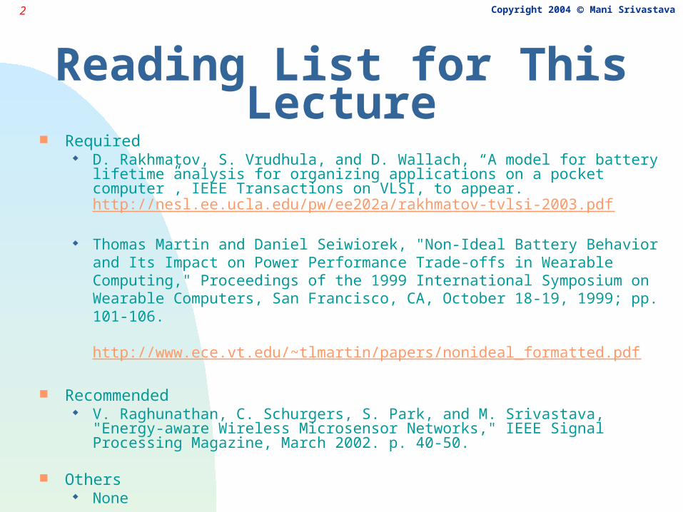
Reading List for This Lecture Required

D. Rakhmatov, S. Vrudhula, and D. Wallach, “A model for battery lifetime analysis for organizing applications on a pocket computer”, IEEE Transactions on VLSI, to appear.http://nesl.ee.ucla.edu/pw/ee202a/rakhmatov-tvlsi-2003.pdf

Thomas Martin and Daniel Seiwiorek, "Non-Ideal Battery Behavior and Its Impact on Power Performance Trade-offs in Wearable Computing," Proceedings of the 1999 International Symposium on Wearable Computers, San Francisco, CA, October 18-19, 1999; pp. 101-106.

http://www.ece.vt.edu/~tlmartin/papers/nonideal_formatted.pdf

Recommended V. Raghunathan, C. Schurgers, S. Park, and M. Srivastava, "Energy-aware

Wireless Microsensor Networks," IEEE Signal Processing Magazine, March 2002. p. 40-50.

Others None


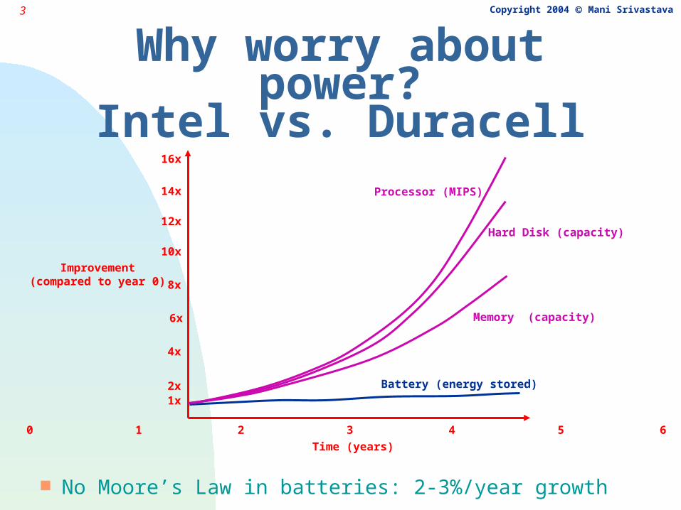
Why worry about power?Intel vs. Duracell

No Moore’s Law in batteries: 2-3%/year growth

Processor (MIPS)

Hard Disk (capacity)

Memory (capacity)

Battery (energy stored)

0 1 2 3 4 5 6

16x

14x

12x

10x

8x

6x

4x

2x1x

Improvement(compared to year 0)

Time (years)


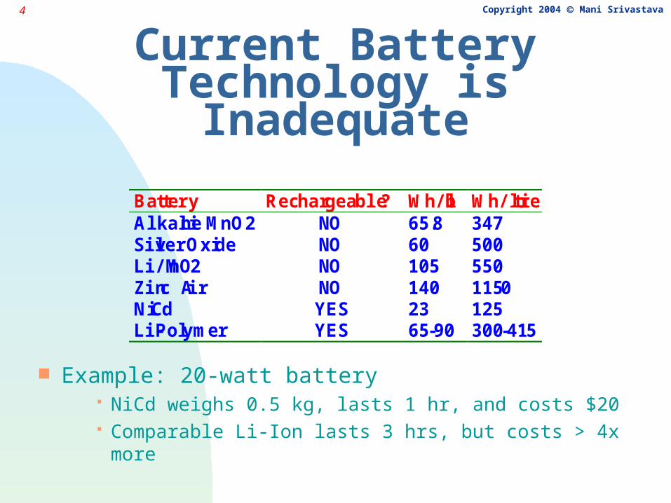
Current Battery Technology is Inadequate

Example: 20-watt battery NiCd weighs 0.5 kg, lasts 1 hr, and costs $20 Comparable Li-Ion lasts 3 hrs, but costs > 4x more

Battery Rechargeable? Wh/lb Wh/litreAlkaline MnO2 NO 65.8 347Silver Oxide NO 60 500Li/MnO2 NO 105 550Zinc Air NO 140 1150NiCd YES 23 125Li-Polymer YES 65-90 300-415


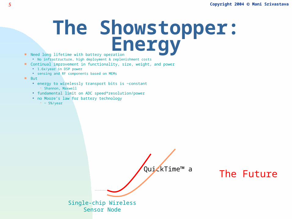
The Showstopper: Energy Need long lifetime with battery operation

No infrastructure, high deployment & replenishment costs Continual improvement in functionality, size, weight, and power

1.6x/year in DSP power sensing and RF components based on MEMs

But energy to wirelessly transport bits is ~constant

Shannon, Maxwell fundamental limit on ADC speed*resolution/power no Moore’s law for battery technology

~ 5%/year

QuickTime™ and aTIFF (Uncompressed) decompressorare needed to see this picture.

QuickTime™ and aTIFF (Uncompressed) decompressorare needed to see this picture.

Single-chip WirelessSensor Node

The Future


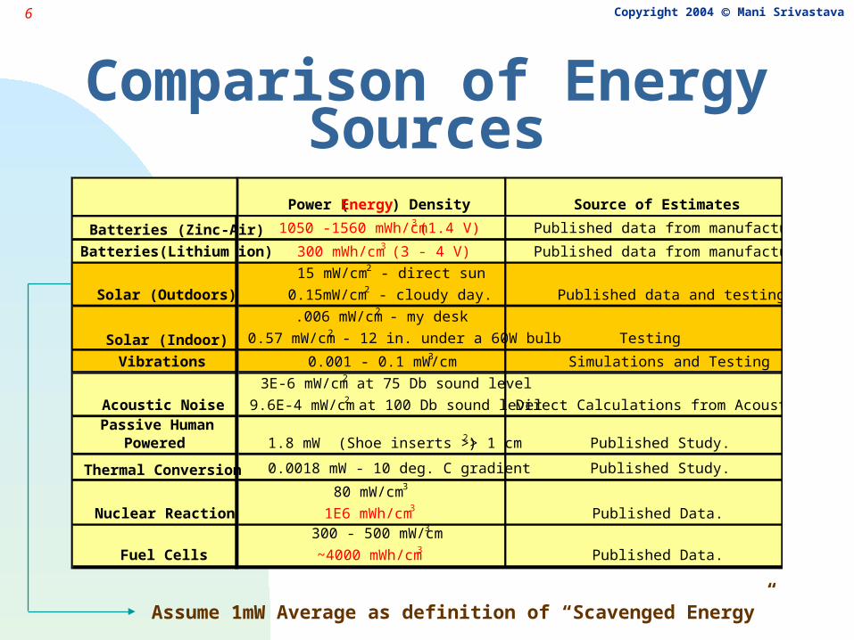
Comparison of Energy Sources

Power (Energy) Density Source of Estimates

Batteries (Zinc-Air) 1050 -1560 mWh/cm3 (1.4 V) Published data from manufacturers

Batteries(Lithium ion) 300 mWh/cm3 (3 - 4 V) Published data from manufacturers

Solar (Outdoors)

15 mW/cm2 - direct sun

0.15mW/cm2 - cloudy day. Published data and testing.

Solar (Indoor)

.006 mW/cm2 - my desk

0.57 mW/cm2 - 12 in. under a 60W bulb Testing

Vibrations 0.001 - 0.1 mW/cm3 Simulations and Testing

Acoustic Noise

3E-6 mW/cm2 at 75 Db sound level

9.6E-4 mW/cm2 at 100 Db sound level Direct Calculations from Acoustic TheoryPassive Human

Powered 1.8 mW (Shoe inserts >> 1 cm2) Published Study.

Thermal Conversion 0.0018 mW - 10 deg. C gradient Published Study.

Nuclear Reaction

80 mW/cm3

1E6 mWh/cm3 Published Data.

Fuel Cells

300 - 500 mW/cm3

~4000 mWh/cm3 Published Data.

Assume 1mW Average as definition of “Scavenged Energy”


Will IC technology alone help?

Speed power efficiency has indeed gone up 10x / 2.5 years for Ps and DSPs in 1990s

degraded before 90s > 100 mW/MIP to < 1 mW/MIP since 1990

IC processes have provided 10x / 8 years since 1965 rest from power conscious IC design in recent years

Lower power for a given function & performance e.g. 1.6x / year reduction since early 80s for DSPs (source TI)


But … Help from IC technology will slow down

e.g. circuit voltage reduction have provided big gains used to be 5V, now around 1.5-2V expected to plateau

Big gains from low-power IC design tricks behind us Strong indications of continued exponential increase in

operating frequency and # of functions we all want color displays, multimedia, wireless comm.,

speech recognition on our PDAs! increase of 10x / 7 yrs in gates, 10x/9 yrs in frequency

Power requirements of wireless communication functions also constrained by Shannon & Maxwell!


IC Technology Trends and Power[source: De99 from Intel]

Transistor scaling Each generation of technology scaling results in 30% reduction in

minimum feature size now mostly “constant electric field” scaling

• gate length, effective electrical gate oxide thickness, and supply voltage scaled by 30%

• use to be constant voltage scaling previously Worst-case sub-threshold leakage current approx. constant

but, have been able to maintain approximately constant drive current per unit width of transistor, at reduced supply voltage

Net result: gate delay reduced by 30%

• areal component of junction capacitances reduced by 30% transistor density is doubled (I.e. die area reduced by 50%) total capacitance on chip reduced by 30% transistor capacitance per unit area increases by 43%


IC Technology Trends and Power(contd.)

Power constant electric field scaling:

43% higher f, 30% less C, 30% less V energy per clock cycle reduces by 65%

• assumes unchanged ave. # of switching transitions per cycle power reduces by 50%

If can’t scale Vdd and Vt (e.g. if electric field < max for reliability) energy reduce by 30% power remains constant can’t add more transistors without increasing power budget! constant voltage scaling was employed until 0.8 micron

But, max power depends not only on technology, but also on implementation (size, frequency, circuit style, microarchitecture etc.)

Metric: “active” or “switched” capacitance (P/V2f) per unit area• scaling theory predicts 43% increase• real life: 30-35% (logic transistor density improvement < x2)


IC Technology Trends and Power (contd.)

Clock frequency doubles every technology generation

instead of 43% (as predicted by 30% gate delay improvement) why?

ave # of gate delays in a clock cycle is reducing (more pipelined) advanced circuit techniques

Die size size of die increases 25% per technology generation new designs add more transistors (integration, complexity)

Interconnect scaling thinner, tighter higher resistance and capacitance more layers interconnect distribution (# of wires vs. length) does not change significantly


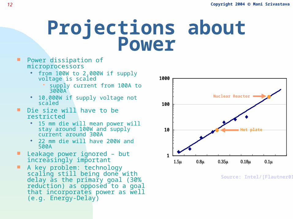
Projections about Power Power dissipation of microprocessors

from 100W to 2,000W if supply voltage is scaled

supply current from 100A to 3000A

10,000W if supply voltage not scaled Die size will have to be restricted

15 mm die will mean power will stay around 100W and supply current around 300A

22 mm die will have 200W and 500A Leakage power ignored – but

increasingly important A key problem: technology scaling

still being done with delay as the primary goal (30% reduction) as opposed to a goal that incorporates power as well (e.g. Energy-Delay)

Source: Intel/[Flautner01]

1

10

100

1000

1.5 0.8 0.35 0.18 0.1

/Watts cm

2

Hot plate

Nuclear Reactor


Barriers to Future Voltage Scaling

Voltage scaling requires threshold voltage Vt to be scaled as well (15% per generation) this increases sub-threshold leakage current impact on power consumption and circuit robustness

Leakage power total leakage current goes up 7.5x per generation leakage power power by 5x soon will become a significant portion of total

active power remains constant for constant die size leakage power, and therefore total power, can be substantially

reduced by cooling Essential to control die temperature power density (W/cm2): 0.6 micron chips surpassed a hot plate!


Barriers to Future Voltage Scaling (contd.)

Circuit performance and robustness scaling V and Vt poses serious challenges to special

circuits such as domino logic, sense amplifiers increase in sub-threshold leakage current impacts bit line

delay on large on-chip caches divergence of logic and cache performance

Single event upsets: soft errors caused by alpha particles in material and cosmic rays reduced capacitance lower energy to flip a bit soft error rate will increase

• adding more capacitance undesirable• memory is typically ECC protected, but not latches, flip-flops

etc.


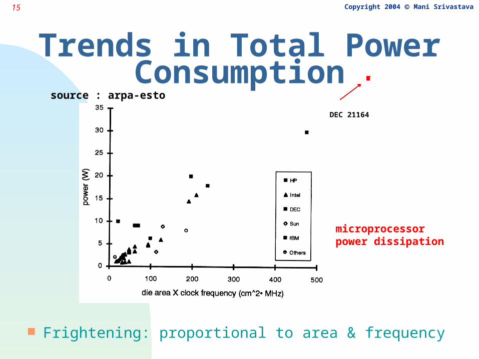
Trends in Total Power Consumption

Frightening: proportional to area & frequency

DEC 21164

source : arpa-esto

microprocessorpower dissipation


System Design for Low Power Need to explicitly design the system with power

consumption or energy efficiency in mind Fortunately, IC technology still continue to help

indirectly by increasing level of integration more and faster transistors can enable low-power

system architectures and design techniques• e.g. system integration on a chip can reduce the

significant circuit I/O power consumption

Energy efficient design of higher layers of the system also help

energy efficient protocols, power-aware apps. etc.


System Design for Low Power (contd.)

Energy efficiency cuts across all system layers entire network, not just the node everything: circuit, logic, software, protocols, algorithms, user

interface, power supply... complex global optimization problem

Need to choose the right metric e.g. individual node vs. network lifetime

Trade-off between energy consumption & QoS optimize energy metric while meeting QoS constraint

Power-awareness, and not just low power right energy at the right time and place


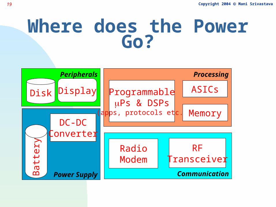
Sources of Power Consumption


Power Supply

Where does the Power Go?B

atte

ry

DC-DCConverter

Communication

RadioModem

RFTransceiver

Processing

ProgrammablePs & DSPs

(apps, protocols etc.) Memory

ASICs

Peripherals

Disk Display


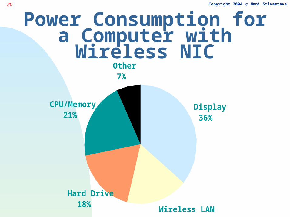
Power Consumption for a Computer with Wireless NIC

Display36%

Wireless LAN18%

Hard Drive18%

CPU/Memory21%

Other7%


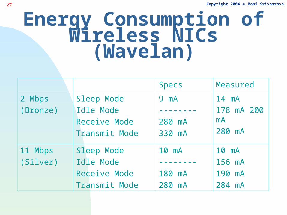
Energy Consumption ofWireless NICs (Wavelan)

Specs Measured

2 Mbps(Bronze)

Sleep ModeIdle ModeReceive ModeTransmit Mode

9 mA--------280 mA330 mA

14 mA178 mA 200 mA280 mA

11 Mbps (Silver)

Sleep ModeIdle ModeReceive ModeTransmit Mode

10 mA--------180 mA280 mA

10 mA156 mA190 mA284 mA


Power Consumption in Post-PC Devices

Pocket computers, PDAs, wireless pads, wireless sensors, pagers, cell phones

Energy and power usage of these devices is markedly different from laptop and notebook computers much wider dynamic range of power demand share of memory, communication and signal processing

subsystems become more important disk storage and displays disappear or become simpler

Design of power-aware higher layer applications and protocols need to be re-evaluated


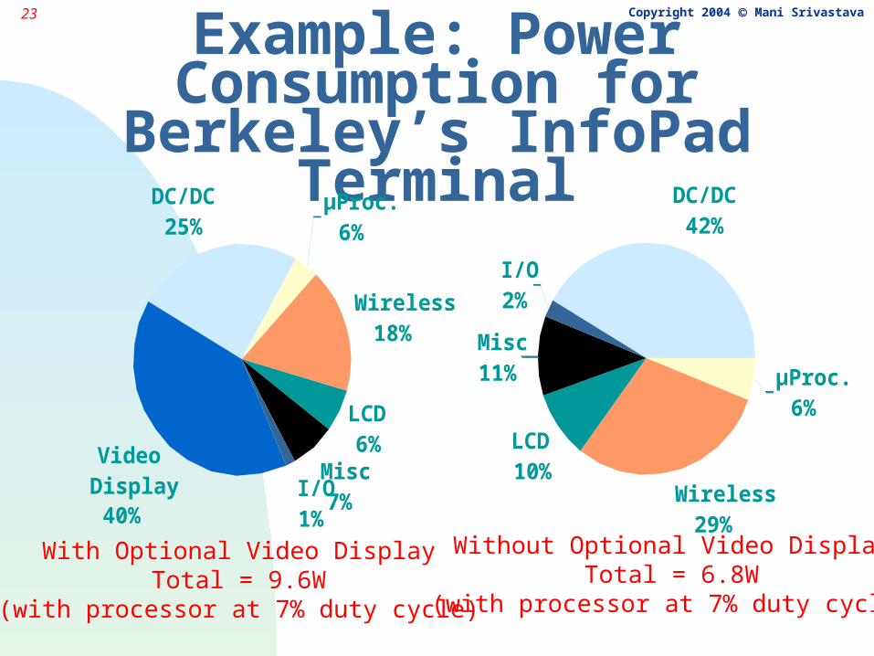
Example: Power Consumption for Berkeley’s InfoPad Terminal

DC/DC25%

LCD6%

I/O1%

Video Display

40%

Wireless18%

µProc.6%

Misc7%

With Optional Video DisplayTotal = 9.6W

(with processor at 7% duty cycle)

DC/DC42%

LCD10%

I/O2%

Wireless29%

µProc.6%

Misc11%

Without Optional Video DisplayTotal = 6.8W

(with processor at 7% duty cycle)


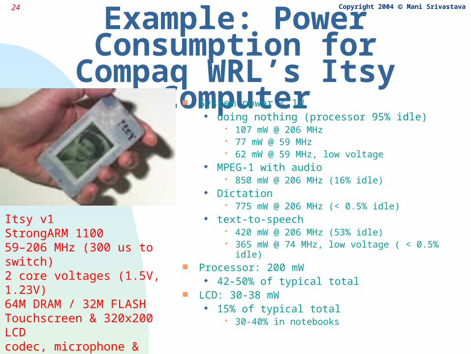
Example: Power Consumption for Compaq WRL’s Itsy Computer

System power < 1W doing nothing (processor 95% idle)

107 mW @ 206 MHz 77 mW @ 59 MHz 62 mW @ 59 MHz, low voltage

MPEG-1 with audio 850 mW @ 206 MHz (16% idle)

Dictation 775 mW @ 206 MHz (< 0.5% idle)

text-to-speech 420 mW @ 206 MHz (53% idle) 365 mW @ 74 MHz, low voltage ( < 0.5% idle)

Processor: 200 mW 42-50% of typical total

LCD: 30-38 mW 15% of typical total

30-40% in notebooks

Itsy v1StrongARM 110059–206 MHz (300 us to switch)2 core voltages (1.5V, 1.23V)64M DRAM / 32M FLASHTouchscreen & 320x200 LCDcodec, microphone & speakerserial, IrDA


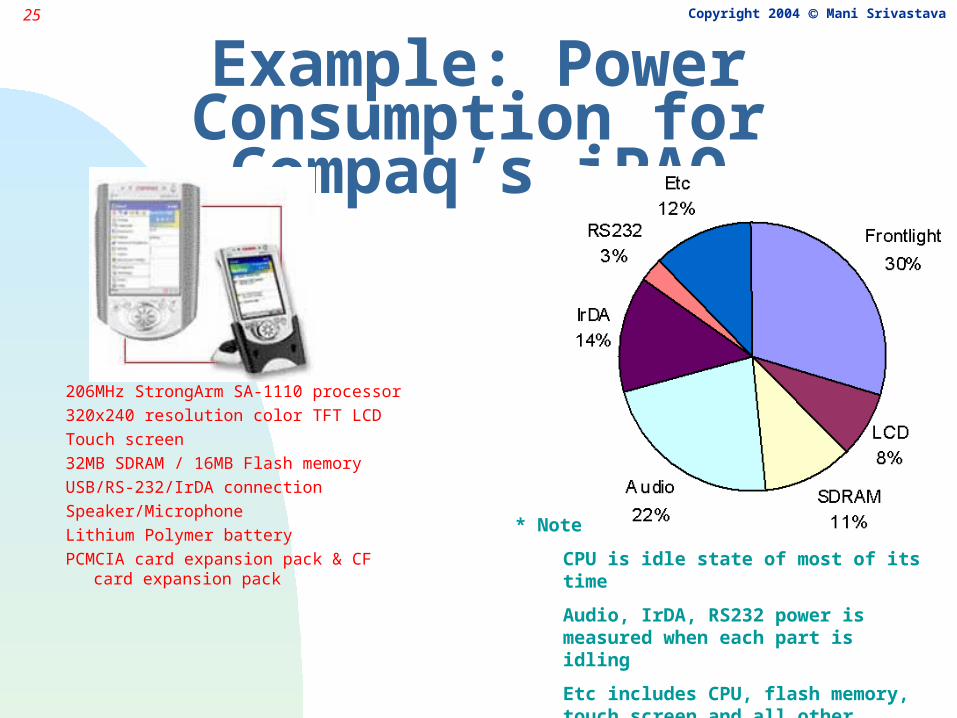
Example: Power Consumption for Compaq’s iPAQ

206MHz StrongArm SA-1110 processor

320x240 resolution color TFT LCD

Touch screen

32MB SDRAM / 16MB Flash memory

USB/RS-232/IrDA connection

Speaker/Microphone

Lithium Polymer battery

PCMCIA card expansion pack & CF card expansion pack

* Note

CPU is idle state of most of its time

Audio, IrDA, RS232 power is measured when each part is idling

Etc includes CPU, flash memory, touch screen and all other devices

Frontlight brightness was 16


The Power Hogs in Post-PC Devices

Wireless modem Rx is comparable, and may be more, than Tx

DC-DC conversion Displays

Handheld flat panel display6.4W Helmet mounted display 4.9W Integrated sight module display 2.6W

Digital subsystem for protocol & applications note: in InfoPad, the processor is used primarily for simple

management of transmit modem schedule Storage peripherals


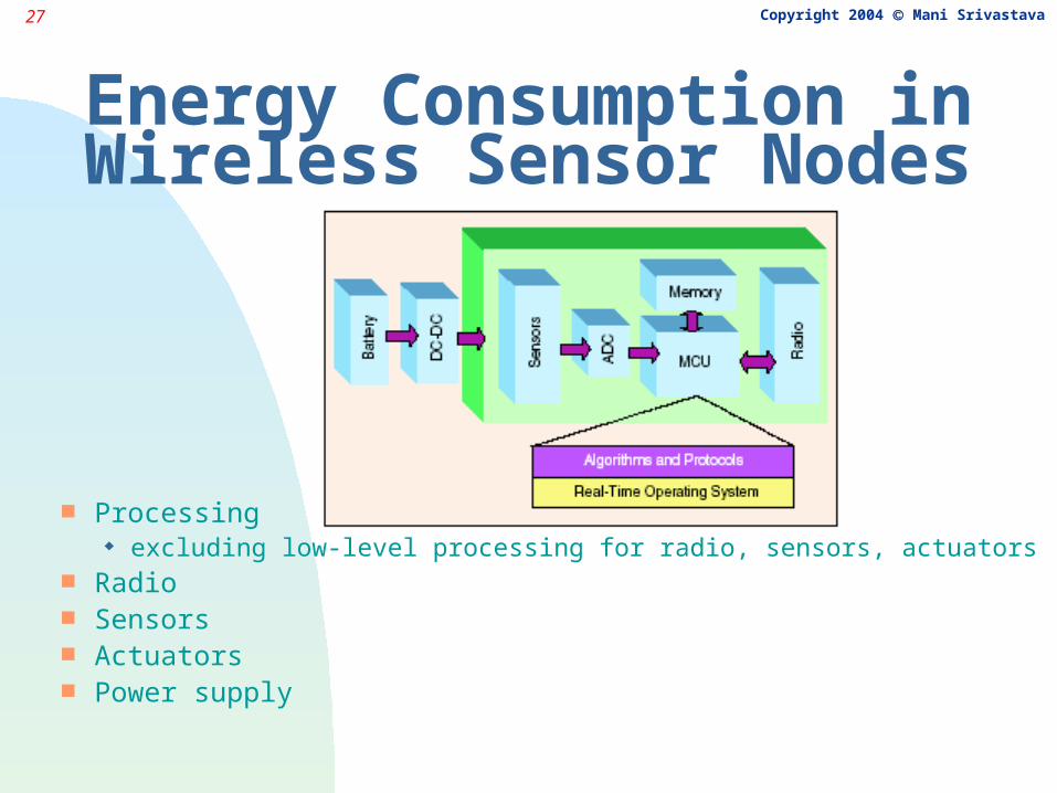
Energy Consumption in Wireless Sensor Nodes

Processing excluding low-level processing for radio, sensors, actuators

Radio Sensors Actuators Power supply


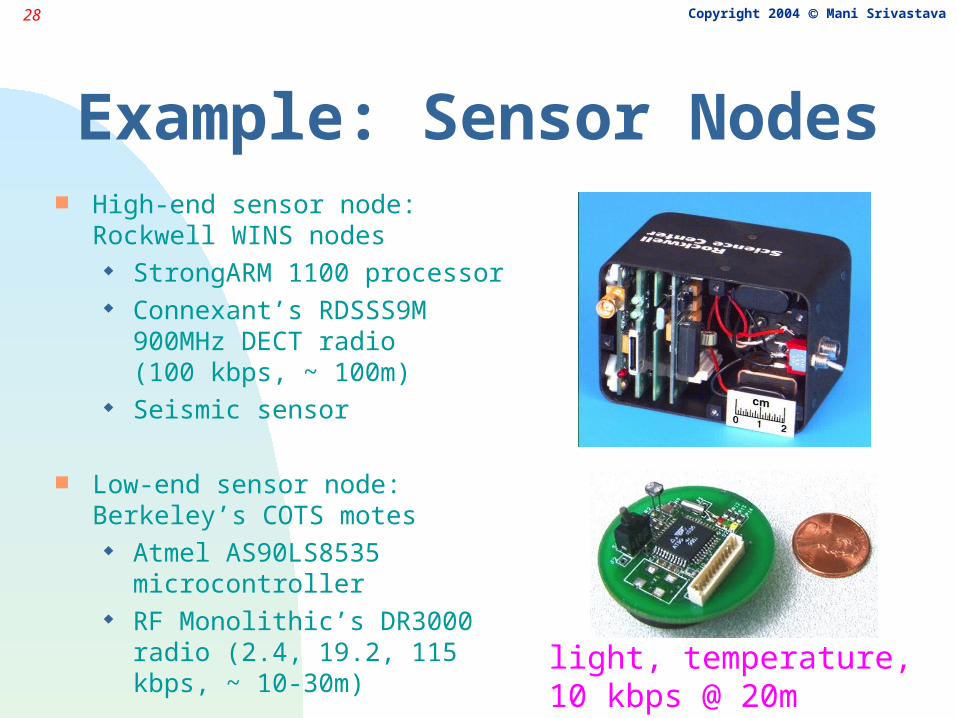
Example: Sensor Nodes High-end sensor node: Rockwell

WINS nodes StrongARM 1100 processor Connexant’s RDSSS9M

900MHz DECT radio(100 kbps, ~ 100m)

Seismic sensor

Low-end sensor node: Berkeley’s COTS motes Atmel AS90LS8535

microcontroller RF Monolithic’s DR3000 radio

(2.4, 19.2, 115 kbps, ~ 10-30m)

light, temperature,10 kbps @ 20m


Processing Common sensor node processors:

Atmel AVR, Intel 8051, StrongARM, XScale, ARM Thumb, SH Risc Power consumption all over the map, e.g.

16.5 mW for ATMega128L @ 4MHz 75 mW for ARM Thumb @ 40 MHz

But, don’t confuse low-power and energy-efficiency! Example

242 MIPS/W for ATMega128L @ 4MHz (4nJ/Instruction) 480 MIPS/W for ARM Thumb @ 40 MHz (2.1 nJ/Instruction)

Other examples: 0.2 nJ/Instruction for Cygnal C8051F300 @ 32KHz, 3.3V 0.35 nJ/Instruction for IBM 405LP @ 152 MHz, 1.0V 0.5 nJ/Instruction for Cygnal C8051F300 @ 25MHz, 3.3V 0.8 nJ/Instruction for TMS320VC5510 @ 200 MHz, 1.5V 1.1 nJ/Instruction for Xscale PXA250 @ 400 MHz, 1.3V 1.3 nJ/Instruction for IBM 405LP @ 380 MHz, 1.8V 1.9 nJ/Instruction for Xscale PXA250 @ 130 MHz, .85V (leakage!)

And, the above don’t even factor in operand size differences! However, need power management to actually exploit energy efficiency

Idle and sleep modes, variable voltage and frequency


Radio Energy per bit in radios is a strong function of desired

communication performance and choice of modulation Range and BER for given channel condition (noise, multipath

and Doppler fading) Watch out: different people count energy differently

E.g. Mote’s RFM radio is only a transceiver, and a lot of low-level

processing takes place in the main CPU While, typical 802.11b radios do everything up to MAC and link

level encryption in the “radio” Transmit, receive, idle, and sleep modes Variable modulation, coding Currently around 150 nJ/bit for short rangeS


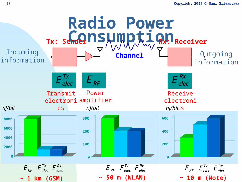
Radio Power ConsumptionTx: Sender Rx: Receiver

ChannelIncominginformation

Outgoinginformation

TxelecE Rx

elecERFETransmit

electronicsReceive

electronicsPower

amplifier

0

2000

4000

6000

8000

0

100

200

300

0

200

400

600

TxelecE Rx

elecERFETxelecE Rx

elecERFETxelecE Rx

elecERFE

nJ/bit nJ/bit nJ/bit

~ 1 km (GSM) ~ 50 m (WLAN) ~ 10 m (Mote)


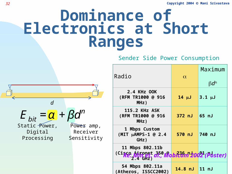
Dominance of Electronics at Short Ranges

d

Static Power,Digital Processing

Power amp,Receiver Sensitivity

Radio Maximum

dn

2.4 KHz OOK(RFM TR1000 @ 916 MHz)

14 J 3.1 J

115.2 KHz ASK(RFM TR1000 @ 916 MHz)

372 nJ 65 nJ

1 Mbps Custom(MIT AMPS-1 @ 2.4 GHz)

570 nJ 740 nJ

11 Mbps 802.11b(Cisco Aironet 350 @ 2.4

GHz)236 nJ 91 nJ

54 Mbps 802.11a(Atheros, ISSCC2002)

14.8 nJ 11 nJ

€

Ebit =α + βdn

Re: Min et. al., Mobicom 2002 (Poster)

Sender Side Power Consumption


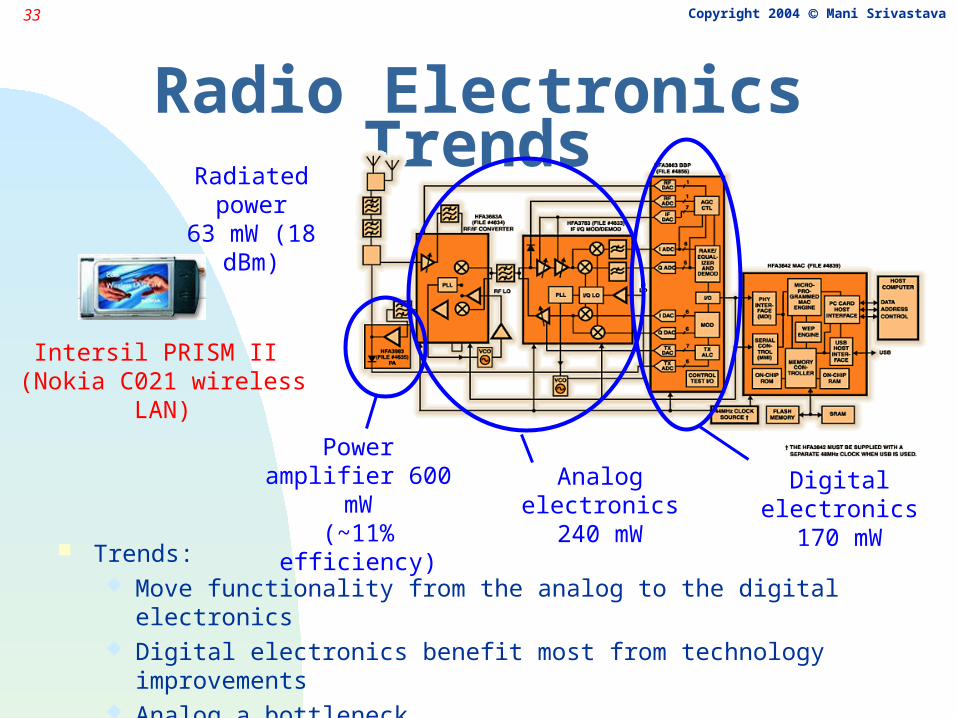
Radio Electronics Trends

Analog electronics240 mW

Digital electronics170 mW

Power amplifier 600 mW

(~11% efficiency)

Intersil PRISM II (Nokia C021 wireless LAN)

Radiated power63 mW (18 dBm)

Trends: Move functionality from the analog to the digital electronics Digital electronics benefit most from technology improvements Analog a bottleneck Digital complexity still increasing (robustness)


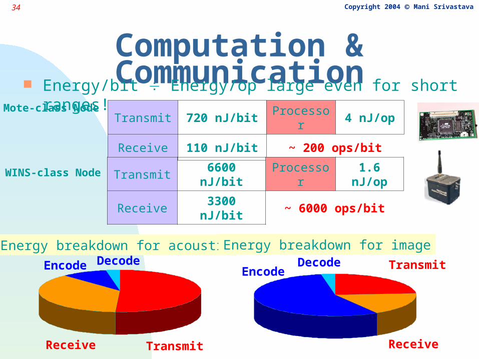
Computation & Communication Energy/bit Energy/op large even for short ranges!

Transmit 720 nJ/bit Processor 4 nJ/op

Receive 110 nJ/bit ~ 200 ops/bit

Mote-class Node

WINS-class Node Transmit 6600 nJ/bit Processor 1.6 nJ/op

Receive 3300 nJ/bit ~ 6000 ops/bit

TransmitReceive

Encode Decode Transmit

Receive

EncodeDecode

Energy breakdown for acoustic Energy breakdown for image


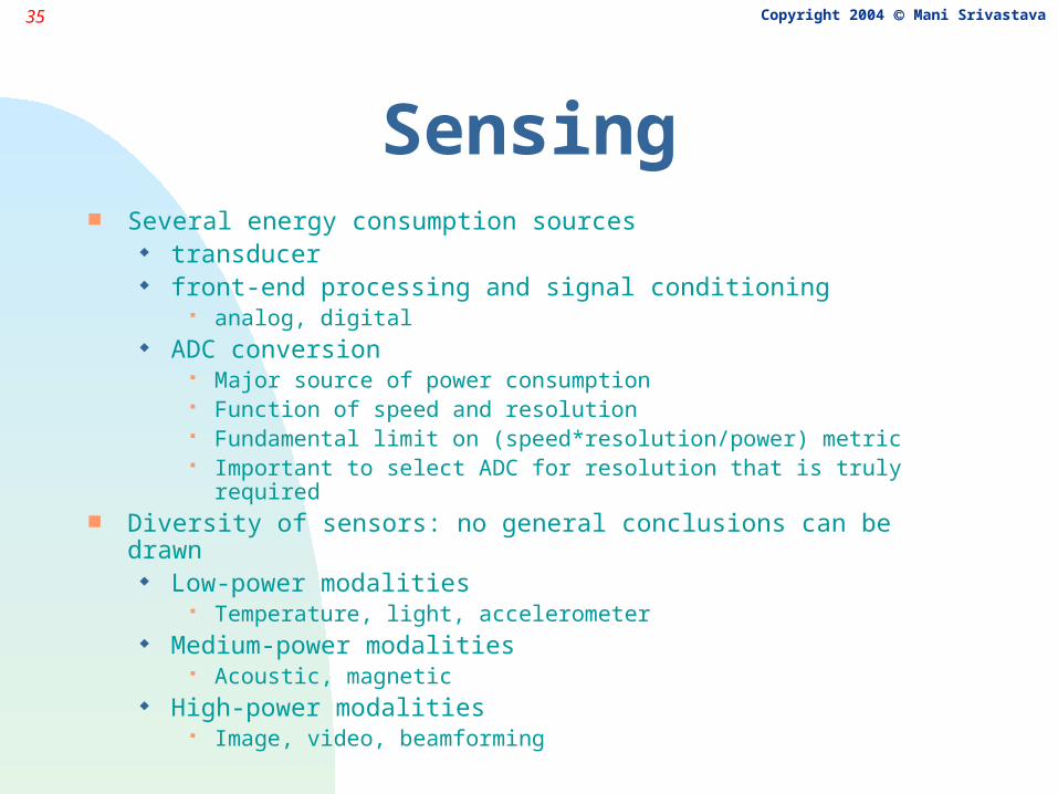
Sensing Several energy consumption sources

transducer front-end processing and signal conditioning

analog, digital ADC conversion

Major source of power consumption Function of speed and resolution Fundamental limit on (speed*resolution/power) metric Important to select ADC for resolution that is truly required

Diversity of sensors: no general conclusions can be drawn Low-power modalities

Temperature, light, accelerometer Medium-power modalities

Acoustic, magnetic High-power modalities

Image, video, beamforming


Actuation Emerging sensor platforms

Mounted on mobile robots Antennas or sensors that can be actuated

Energy trade-offs not yet studied Some thoughts:

Actuation often done with fuel, which has much higher energy density than batteries

E.g. anecdotal evidence that in some UAVs the flight time is longer than the up time of the wireless camera mounted on it

Actuation done during boot-up or once in a while may have significant payoffs

E.g. mechanically repositioning the antenna once may be better than paying higher communication energy cost for all subsequent packets

E.g. moving a few nodes may result in a more uniform distribution of node, and thus longer system lifetime


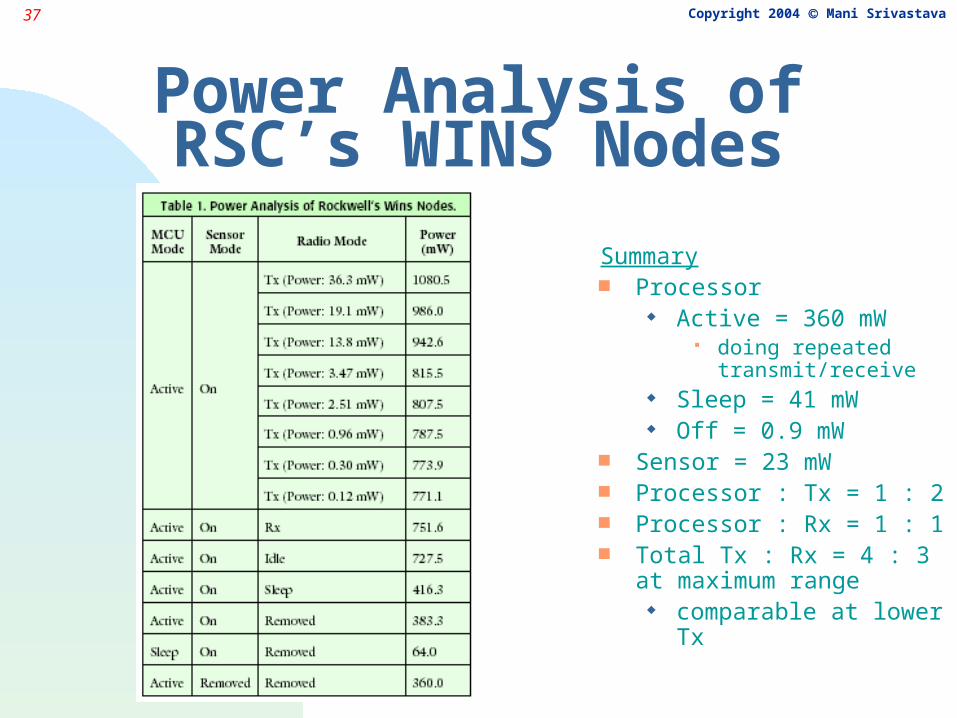
Power Analysis of RSC’s WINS Nodes

Summary Processor

Active = 360 mW doing repeated

transmit/receive Sleep = 41 mW Off = 0.9 mW

Sensor = 23 mW Processor : Tx = 1 : 2 Processor : Rx = 1 : 1 Total Tx : Rx = 4 : 3 at

maximum range comparable at lower Tx


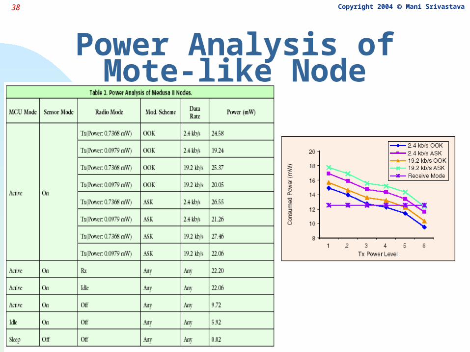
Power Analysis of Mote-like Node


Some Observations Using low-power components and trading-off unnecessary performance for power

savings can have orders of magnitude impact Node power consumption is strongly dependent on the operating mode

E.g. WINS consumes only 1/6-th the power when MCU is asleep as opposed to active

At short ranges, the Rx power consumption > T power consumption multihop relaying not necessarily desirable

Idle radio consumes almost as much power as radio in Rx mode Radio needs to be completely shut off to save power as in sensor networks idle

time dominates MAC protocols that do not “listen” a lot

Processor power fairly significant (30-50%) share of overall power In WINS node, radio consumes 33 mW in “sleep” vs. “removed”

Argues for module level power shutdown Sensor transducer power negligible

Use sensors to provide wakeup signal for processor and radio Not true for active sensors though…


Metrics for Power

Power sets battery life in hours problem: power frequency (slow the system!)

Energy per operation fixes obvious problem with the power metric but can cheat by doing stuff that will slow the chip

– Energy/op = Power * Delay/op

Metric should capture both energy and performance: e.g. Energy/Op * Delay/Op

Energy*Delay = Power*(Delay/Op)2


Communication vs. Computing A good measure is J/bit vs. J/ instruction Examples

Rockwell WINS nodes: 1500 to 2700 Medusa (similar to UCB’s motes): 220 to 2900 Sensoria’s WINS NG 2.0 nodes: ~ 1400

But watch out: not all instructions are the same: 8-bit vs. 32-bit not all bits are the same: distance, error probability


Sources of Power: Batteries


Battery Characteristics

Important characteristics: energy density (Wh/liter) and specific energy (Wh/kg) power density (W/liter) and specific power (W/kg) open-circuit voltage, operating voltage cut-off voltage (at which considered discharged) shelf life (leakage) cycle life

The above are decided by “system chemistry” advances in materials and packaging have resulted in

significant changes in older systems– carbon-zinc, alkaline manganese, NiCd, lead-acid

new systems– primary and secondary (rechargeable) Li– secondary zinc-air, Ni-metal hydride


Modeling the Battery Behavior

Theoretical capacity of battery is decided by the amount of the active material in the cell

batteries often modeled as buckets of constant energy – e.g. halving the power by halving the clock frequency is

assumed to double the computation time while maintaining constant computation per battery life

In reality, delivered or nominal capacity depends on how the battery is discharged

discharge rate (load current) discharge profile and duty cycle operating voltage and power level drained


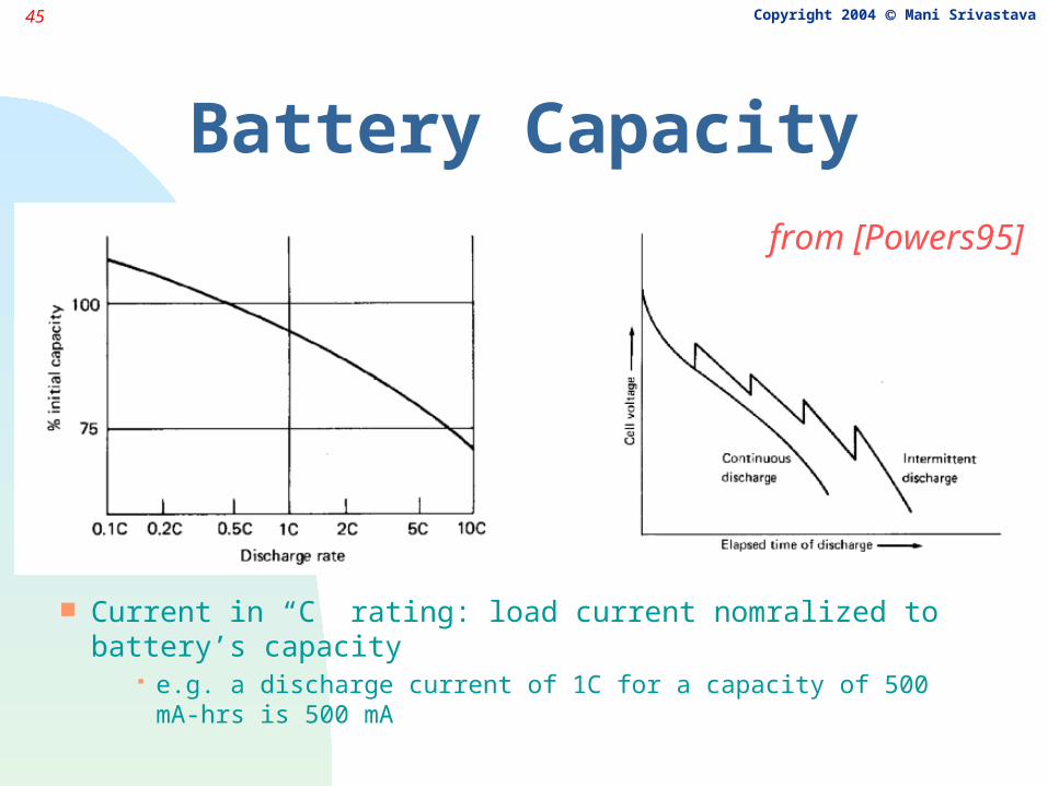
Battery Capacity

Current in “C” rating: load current nomralized to battery’s capacity e.g. a discharge current of 1C for a capacity of 500 mA-hrs is 500 mA

from [Powers95]


Battery Capacity vs. Discharge Current

Amount of energy delivered is decreased as the current (rate at which power is drawn) is increased

rated as ampere hours or watt hours when discharged at a specific rate to a specific cut-off voltage

– primary cells rated at a current which is 1/100th of the capacity in ampere hours (C/100)

– secondary cells are rated at C/20 or C/10 At high currents, the diffusion process that moves new

active material from electrolytes to the electrode cannot keep up

concentration of active material at cathode drops to zero, and cell voltage goes down below cut-off

even though active material in cell is not exhausted!


Battery Capacity vs. Discharge Current: Peukert’s Formula

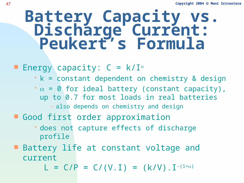
Energy capacity: C = k/I k = constant dependent on chemistry & design = 0 for ideal battery (constant capacity), up to 0.7

for most loads in real batteries– also depends on chemistry and design

Good first order approximation does not capture effects of discharge profile

Battery life at constant voltage and currentL = C/P = C/(V.I) = (k/V).I-(1+)


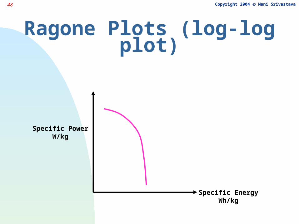
Ragone Plots (log-log plot)

Specific PowerW/kg

Specific EnergyWh/kg


Amount of Computation during Battery Lifetime

Consider a system modification that changes performance by factor n and power by factor x

total work (= speed x lifetime) will change by n.x -(1+)

e.g. reducing the clock frequency by xN reduces power by xN (N>1) & reduces performance by xN,

work done changes by (1/N)x(1/N) -(1+) = N

– > 1 for >0 however, can’t just go on reducing frequency

– static power dissipated even at zero frequency– P = V.I = V.(S+Df)

optimum frequency to maximize computation problem: system performance does not change linearly with

frequency (e.g. memory bottlenecks)


Alternate Equivalent View of the Battery

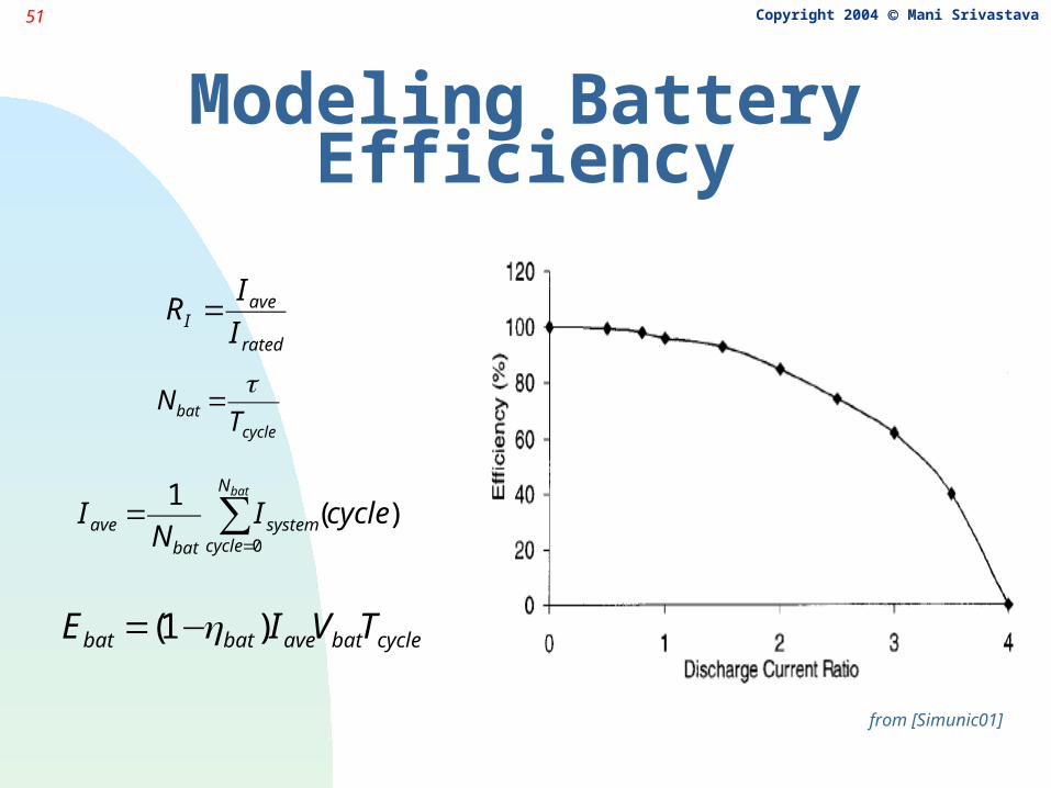
Manufacturer’s often give battery efficiency (%) vs. discharge rate (or discharge current ratio) discharge rate = Iave/Irated

Battery cannot respond to instantaneous changes in current so, a time constant used to calculate Iave

Given actual energy drawn by the circuit, one can use the battery efficiency to calculate the actual depletion in the stored energy in the battery

Example: battery efficiency is 60% and its rated capacity is 100 mAh @ 1V computed average DC-DC current of 300 mA would drain the

battery in 12 min, while at 100% efficiency it would last 1 hr


Modeling Battery Efficiency

rated

aveI I

IR =

cyclebat TN

=

∑=

=batN

cyclesystem

batave cycleI

NI

0

)(1

cyclebatavebatbat TVIE )1( η−=

from [Simunic01]


Digression:Metrics to Relate Power and Performance

MIPS/Watt: millions of instructions per Joule problem: running faster gives better MIPS/Watt increasing frequency by N

MIPS go up by xN power goes up < xN due to static power MIPS/Watt will increase!

W/Spec2 has similar problem Total computation during battery lifetime is better

shows diminishing returns of increasing frequency


Capacity & Variable Discharge Current: Constant vs. Pulsed

Capacity can be extended by draining power in short discharge periods separated by rest periods

also works with constant background current Battery relaxes and partially recovers the active

material lost during the current impulse longer the rest period, the better is the recovery longer rest period needed as the discharge depth

becomes greater battery voltage also goes back up


Benefits of Pulsed Discharge

Higher specific power for a given specific energy impulses of several times the limiting current value

can be obtained by choosing short pulses and long rest periods

Higher specific energy for a given specific power ideally, want specific energy = theoretical capacity depends on pulse and rest periods


Exploiting Pulse Discharge

Gain in battery life if system shutdown is done taking into account the pulse discharge

Examples: protocols in case of radios where power during

transmission is a lot higher than during receive and idle periods

shutdown of CPUs and variable speed CPUs shutdown of disks

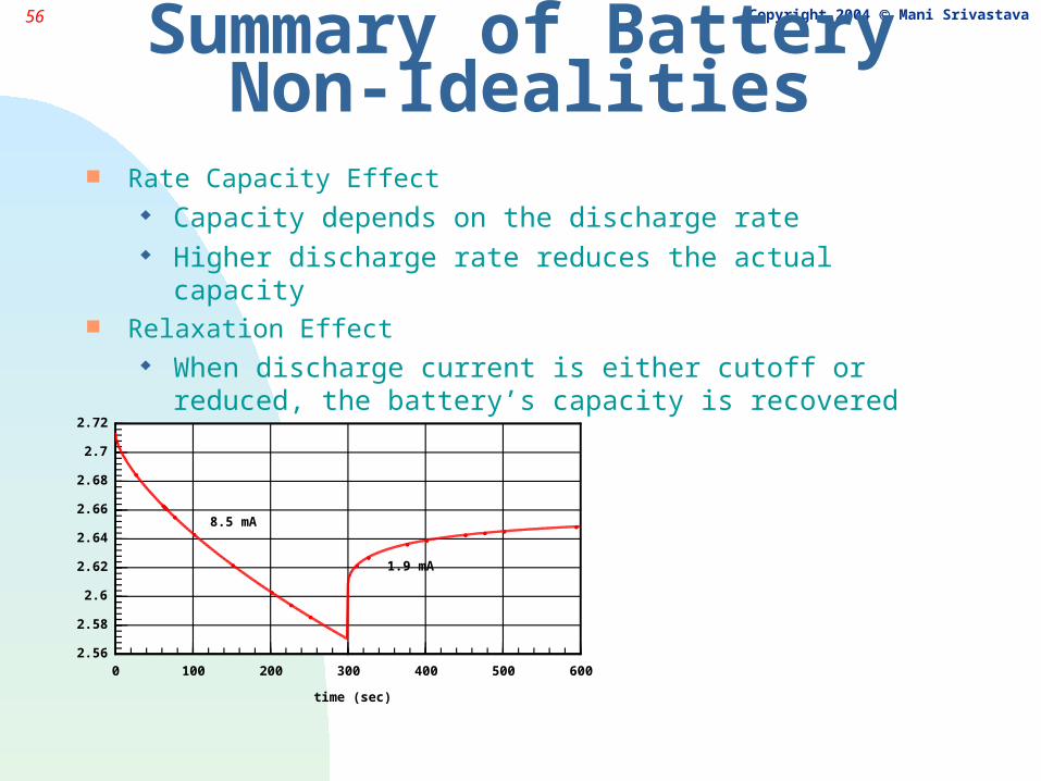
56 Copyright 2004 Mani SrivastavaSummary of BatteryNon-Idealities

Rate Capacity Effect Capacity depends on the discharge rate Higher discharge rate reduces the actual capacity

Relaxation Effect When discharge current is either cutoff or reduced, the battery’s

capacity is recovered

0 100 200 300 400 500 600

time (sec)

2.56

2.58

2.6

2.62

2.64

2.66

2.68

2.7

2.72

Voltage (V)

8.5 mA

1.9 mA


Battery Modeling Predict battery lifetime given a load profile Many battery models

Model electrochemical processes in the battery Solve system of PDEs, e.g. Berkeley’s DUALFOIL Accurate but long simulation times and large number of

parameters (e.g. > 50 with DUALFOIL) Not easy to use in an optimization tool

Abstract representation of batteries E.g. Markov chain No physics or chemistry based justification Not easy to use in an optimization tool

Analytical models Capture key factors of battery performance E.g model by Rakhmatov & Vrudhula @ U. Arizona


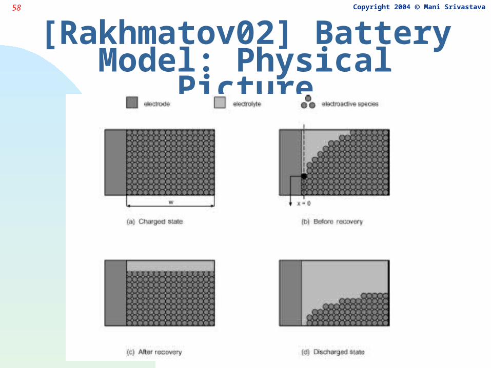
[Rakhmatov02] Battery Model: Physical Picture


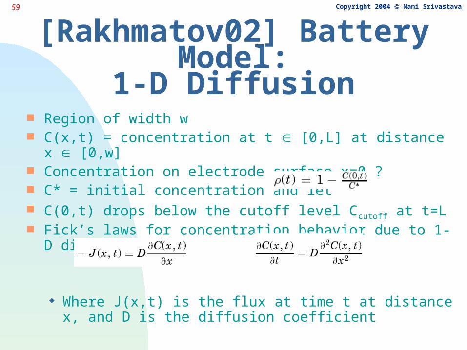
[Rakhmatov02] Battery Model:1-D Diffusion

Region of width w C(x,t) = concentration at t [0,L] at distance x [0,w] Concentration on electrode surface x=0 ? C* = initial concentration and let C(0,t) drops below the cutoff level Ccutoff at t=L Fick’s laws for concentration behavior due to 1-D diffusion

Where J(x,t) is the flux at time t at distance x, and D is the diffusion coefficient


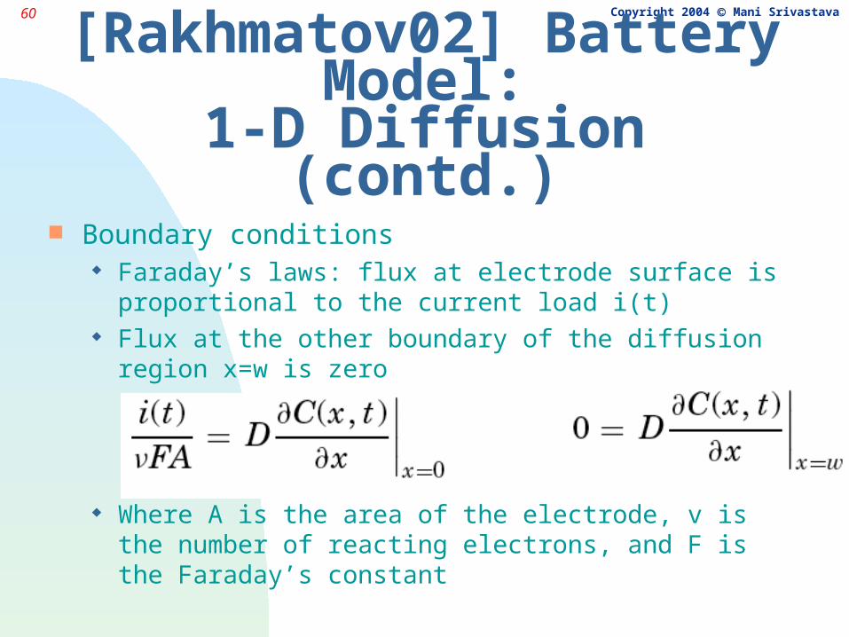
[Rakhmatov02] Battery Model:1-D Diffusion (contd.)

Boundary conditions Faraday’s laws: flux at electrode surface is proportional to

the current load i(t) Flux at the other boundary of the diffusion region x=w is

zero

Where A is the area of the electrode, v is the number of reacting electrons, and F is the Faraday’s constant



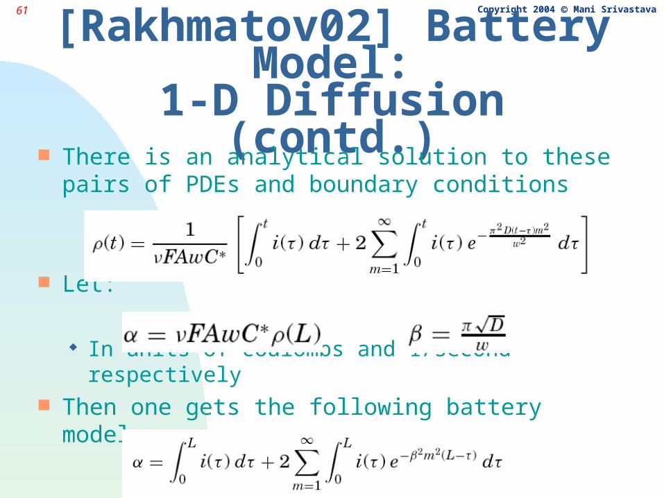
There is an analytical solution to these pairs of PDEs and boundary conditions

Let:

In units of coulombs and 1/second respectively Then one gets the following battery model



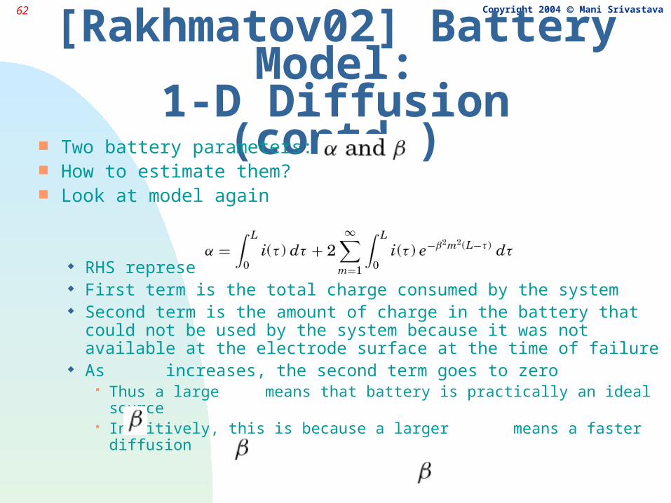
Two battery parameters: How to estimate them? Look at model again

RHS represents the capacity of the battery First term is the total charge consumed by the system Second term is the amount of charge in the battery that could

not be used by the system because it was not available at the electrode surface at the time of failure

As increases, the second term goes to zero Thus a large means that battery is practically an ideal source Intuitively, this is because a larger means a faster diffusion


Estimating and

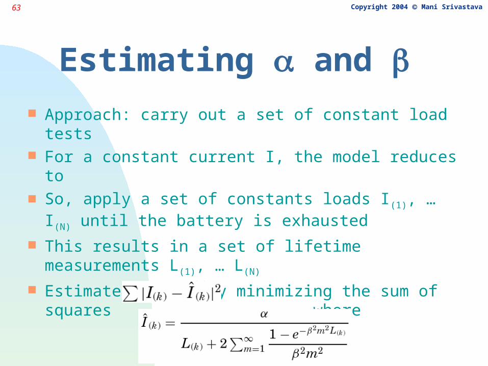
Approach: carry out a set of constant load tests For a constant current I, the model reduces to So, apply a set of constants loads I(1), … I(N) until

the battery is exhausted This results in a set of lifetime measurements

L(1), … L(N) Estimate and by minimizing the sum of

squares where


Alternatives to Batteries?

Small batteries are the only choice for consumer products up to 20W

But heavy expensive expire without warning require replacement (disposal problem) or

recharging (time problem) Are there alternatives?


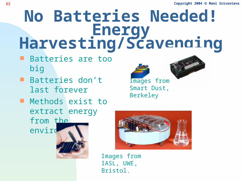
No Batteries Needed!Energy Harvesting/Scavenging

Batteries are too big Batteries don’t last

forever Methods exist to extract

energy from the environment

Images from Smart Dust, Berkeley

Images from IASL, UWE, Bristol.


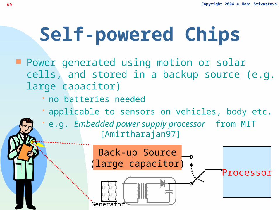
Self-powered Chips Power generated using motion or solar cells, and

stored in a backup source (e.g. large capacitor) no batteries needed applicable to sensors on vehicles, body etc. e.g. Embedded power supply processor from MIT

[Amirtharajan97]

Back-up Source(large capacitor)

Generator

Processor

67 Copyright 2004 Mani SrivastavaExample: Scavenging from Motion

Media Lab’s “Parasitic Power Harvesting” project for devices built into a shoe http://www.media.mit.edu/resenv/power.html piezoelectric shoe inserts, shoe-mounted rotary

magnetic generator 20-80 mW of peak power during brisk walk, 1-2 mW average

a system had been built around the piezoelectric shoes that periodically broadcasts a 12-bit digital RFID as the bearer walks

charge stored in a capacitor over several footsteps and then discharged during RFID transmission every 3-5 footsteps


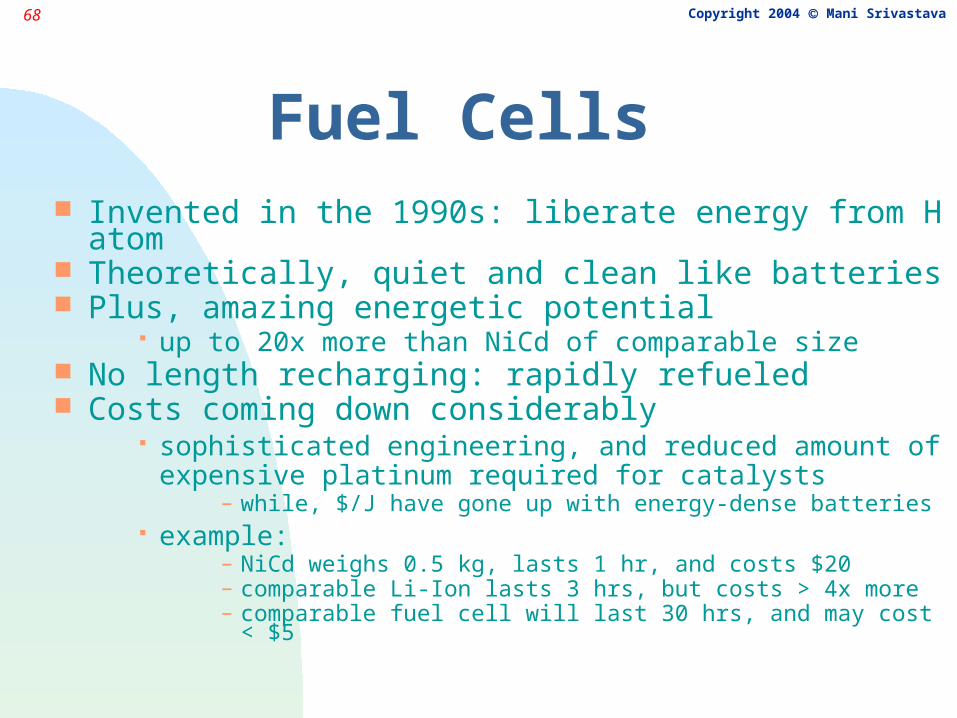
Fuel Cells Invented in the 1990s: liberate energy from H atom Theoretically, quiet and clean like batteries Plus, amazing energetic potential

up to 20x more than NiCd of comparable size No length recharging: rapidly refueled Costs coming down considerably

sophisticated engineering, and reduced amount of expensive platinum required for catalysts

– while, $/J have gone up with energy-dense batteries example:

– NiCd weighs 0.5 kg, lasts 1 hr, and costs $20– comparable Li-Ion lasts 3 hrs, but costs > 4x more– comparable fuel cell will last 30 hrs, and may cost < $5


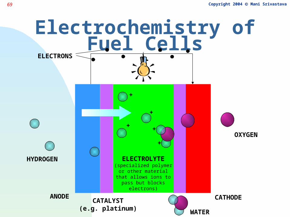
Electrochemistry of Fuel Cells

ELECTROLYTE(specialized polymer

or other materialthat allows ions topass but blocks

electrons)

ANODE CATHODECATALYST(e.g. platinum)

HYDROGEN

OXYGEN

+

+

+

+

+

ELECTRONS

WATER


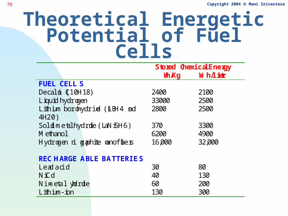
Theoretical Energetic Potential of Fuel Cells

Stored Chemical Energy Wh/Kg Wh/liter

FUEL CELLSDecalin (C10H18) 2400 2100Liquid hydrogen 33000 2500Lithium borohydride (LiBH4 and4H20)

2800 2500

Solid metal hydride (LaNi5H6) 370 3300Methanol 6200 4900Hydrogen in graphite nanofibers 16,000 32,000

RECHARGEABLE BATTERIESLead acid 30 80NiCd 40 130Ni-metal hydride 60 200Lithium-ion 130 300


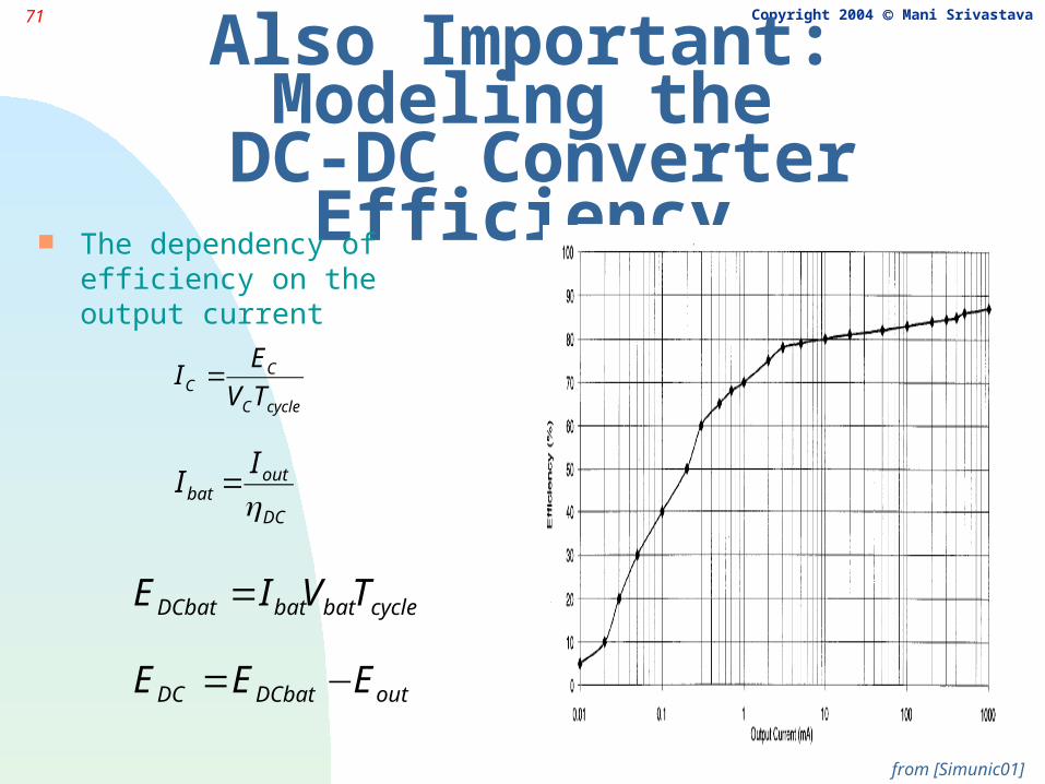
Also Important: Modeling the DC-DC Converter Efficiency

The dependency of efficiency on the output current

cycleC

CC TV

EI =

DC

outbat

II

η=

cyclebatbatDCbat TVIE =

outDCbatDC EEE −=

from [Simunic01]


Summary

Batteries improve very slowly The hunt for disruptive technology is on

Better sources Scavenging & harvesting

Until then: Exploit interesting non-linearities and dynamics that are

exhibited by batteries Resource allocation and scheduling can be made battery-

aware (task scheduling by OS in processors, packet scheduling by MAC in radios)

Documents

Mani Srivastava UCLA - EE Department Room: 6731-H Boelter Hall Email: [email protected] Tel: 310-267-2098 WWW: mbs Copyright 2004