Embed Size (px)
Citation preview

MANEUVER ESTIMATION MODEL FOR
GEOSTATIONARY ORBIT DETERMINATION
THESIS
Brian J. Hirsch
AFIT/GA/ENY/06-J01
DEPARTMENT OF THE AIR FORCE AIR UNIVERSITY
AIR FORCE INSTITUTE OF TECHNOLOGY
Wright-Patterson Air Force Base, Ohio
APPROVED FOR PUBLIC RELEASE; DISTRIBUTION UNLIMITED

The views expressed in this thesis are those of the author and do not reflect the official policy or position of the United States Air Force, Department of Defense, or the United States Government.

AFIT/GA/ENY/06-J01
MANEUVER ESTIMATION MODEL FOR GEOSTATIONARY ORBIT DETERMINATION
THESIS
Presented to the Faculty
Department of Aeronautics and Astronautics
Graduate School of Engineering and Management
Air Force Institute of Technology
Air University
Air Education and Training Command
In Partial Fulfillment of the Requirements for the
Degree of Master of Science in Astronautical Engineering
Brian J. Hirsch
June 2006
APPROVED FOR PUBLIC RELEASE; DISTRIBUTION UNLIMITED.

AFIT/GA/ENY/06-J01
MANEUVER ESTIMATION MODEL FOR GEOSTATIONARY ORBIT DETERMINATION
Brian J. Hirsch
Approved: ____________________________________ Dr. William E. Wiesel date Advisor ____________________________________ Lt Col Kerry D. Hicks date Committee Member ____________________________________ Lt Col Nathan A. Titus date Committee Member

AFIT/GA/ENY/06-J01
Abstract
As an increasing number of geostationary satellites fill a limited number of orbital
slots, collocation of satellites leads to a risk of close approach or misidentification. The
ability to detect maneuvers made by these satellites using optical observations can help to
prevent these problems. Such a model has already been created and tested using data
from the Air Force Maui Optical and Supercomputing site.
The goal of this research was to create a more robust model which would reduce
the amount of data needed to make accurate maneuver estimations. The Clohessy-
Wiltshire equations were used to model the relative motion of a geostationary satellite
about its intended location and a nonlinear least squares algorithm was developed to
estimate the satellite trajectories.
iv

Acknowledgements
I would like to thank my thesis advisor, Dr. William Wiesel, for his guidance and
all the knowledge he imparted along the way. I appreciate his patience throughout my
near daily visits to his office. I’m thankful for every one of those office visits as I always
left understanding astronautics a little better than when I came.
A sincere group of friends, especially friends with programming experience, is
always a blessing to have. I am grateful to have such a group to offer their support
throughout this research.
Finally, I’d like to thank my parents for being both a source of encouragement
and an ear to which I could always vent my frustrations. More than anyone else, they’ve
helped make me who I am today, and much of my scholastic success is due to the work
ethic they’ve instilled upon me.
Brian J. Hirsch
v

Table of Contents Page
Abstract ...................................................................................................................... iv Acknowledgements ......................................................................................................v Table of Contents ....................................................................................................... vi List of Figures ........................................................................................................... viii List of Symbols ............................................................................................................x I. Introduction ...........................................................................................................1 1.1 Background.....................................................................................................1 1.2 Problem Statement ..........................................................................................2 1.3 Research Objectives........................................................................................2 II. Literature Review..................................................................................................3 2.1 Observation Geometry ...................................................................................3 2.1.1 The Celestial Sphere .........................................................................3 2.1.2 Frames of Reference .........................................................................4 2.2 Orbital Perturbations......................................................................................5 2.2.1 Geostationary Orbit...........................................................................5 2.2.2 Perturbations from Ideal GEO Orbits ...............................................6 2.3 Relative Motion .............................................................................................7 2.3.1 Applications to Geostationary Satellites...........................................7 2.3.2 Clohessy-Wiltshire Equations...........................................................8 2.4 Least Squares Approximation......................................................................10 2.4.1 Principle of Maximum Likelihood..................................................10 2.4.2 Linear Least Squares.......................................................................11 2.4.3 Nonlinear Least Squares .................................................................12 III. Methodology......................................................................................................15 3.1 Determining Orbit Geometry ......................................................................15 3.1.1 Application of Clohessy-Wiltshire Equations ................................15 3.1.2 Observations to State Conversion...................................................16 3.2 Test Data Generator .....................................................................................19 3.2.1 Non-maneuver Test Data ................................................................19 3.2.2 Maneuver Test Data........................................................................23 3.3 Non-maneuver Model ..................................................................................26 3.4 Maneuver Model..........................................................................................27 3.4.1 Separating Data with an East-West Maneuver ...............................28 3.4.2 Separating Data with a North-South Maneuver..............................36 3.4.3 Corrections to Data Separation Models ..........................................40
vi

Page
3.4.4 Determining Possible Maneuver Times..........................................44 3.4.5 Choosing Correct Maneuver Time..................................................48 3.4.6 Non-maneuver Data in the Maneuver Model .................................50 IV. Simulation Results ...............................................................................................51 4.1 Response to East-West Maneuvers .............................................................51 4.1.1 Response to Ideal Data....................................................................51 4.1.2 Response to Increasingly Uncertain Data .......................................55 4.1.3 Limits on Maneuver Time ..............................................................59 4.2 Response to North-South Maneuvers..........................................................63 4.2.1 Response to Uncertain Data............................................................66 V. Conclusion ..........................................................................................................69 5.1 Summary .....................................................................................................69 5.2 Conclusions .................................................................................................69 5.2.1 Results Summary ............................................................................69 5.2.2 Future Work ....................................................................................71 Appendix A. Derivation of Linearized Observation Relation ....................................73 Appendix B. MATLAB Code - test_data_generator2.m.............................................76 Appendix C. MATLAB Code - man_data_generator2.m...........................................79 Appendix D. MATLAB Code - NLS_nonman_algorithm.m .....................................82 Appendix E. MATLAB Code - NLS_man_algorithm.m............................................85 Appendix F. MATLAB Code - NLS_loop.m .............................................................91 Appendix G. MATLAB Code - obs_matrix.m ...........................................................94 Appendix H. MATLAB Code - pre_post_man_separate.m .......................................97 Appendix I. MATLAB Code - dec_man_check.m...................................................104 Appendix J. MATLAB Code - ra_man_check.m .....................................................105 Appendix K. MATLAB Code - possible_man_times.m ..........................................107 Bibliography ..............................................................................................................110 Vita.............................................................................................................................111
vii

List of Figures
Figure Page 2.1 The Celestial Sphere ...........................................................................................4 3.1 Observation Geometry ......................................................................................17 3.2 Sample of Non-maneuver Test Data.................................................................20 3.3 Sample of Truncated Non-maneuver Test Data................................................22 3.4 Sample of Maneuver Test Data.........................................................................24 3.5 Sample of Truncated Maneuver Test Data .......................................................25 3.6 NLS curve fitted to first data set .......................................................................29 3.7 Discrete NLS curve fitted to first data set.........................................................30 3.8 Difference between NLS Fit and Observed Data for an E-W maneuver..........31 3.9 Scaled Difference between NLS Fit and Observed Data..................................32 3.10 Slope between the Data Points from Figure 3.9 ...............................................33 3.11 Percentage Difference between the Data Points from Figure 3.10...................34 3.12 Observation Data Separated into Pre-maneuver and Post-maneuver Sets........35 3.13 NLS curve fitted to first data set .......................................................................37 3.14 Difference between NLS Fit and Observed Data for a N-S maneuver.............38 3.15 Percentage Difference between the Data Points from Figure 3.14...................39 3.16 Slope between the Data Points Using Noisy Data ............................................41 3.17 Modified Slope between the Data Points Using Noisy Data ............................41 3.18 Flow Chart of Data Separation Method for E-W Maneuver.............................42 3.19 Flow Chart of Data Separation Method for N-S Maneuver..............................43 3.20 Percentage Difference between the Data Points Using Noisy Data .................43
viii

Figure Page 3.21 Modified Percentage Difference between the Data Points Using Noisy Data..44 3.22 Sample of Pre-maneuver and Post-maneuver NLS Fits ...................................45 3.23 Close-up of NLS Fits Showing Possible Maneuver Intersections ....................46 3.24 Difference between Pre-maneuver and Post-maneuver Fits .............................47 3.25 Intersection Region of Pre-maneuver and Post-maneuver Difference Plot ......47 4.1 Test Data with 3 cm/s E-W Maneuver at 5.5 days ...........................................52 4.2 Response to Test Data from Figure 4.1 ............................................................53 4.3 Test Data with 1 cm/s E-W Maneuver at 6 days ..............................................54 4.4 Incorrect separation for 1.5 cm/s Maneuver at 6 days ......................................55 4.5 Incorrect Estimated Trajectory for 1.5 cm/s Maneuver at 6 days.....................56 4.6 Model’s Response to Data with 2 Arcsecond Uncertainty ...............................58 4.7 Test Data with 7 cm/s E-W Maneuver at 8.5 days ...........................................59 4.8 Example of Poor Post-maneuver Fit .................................................................60 4.9 Estimated Trajectory of Poor Post-maneuver Fit..............................................61 4.10 Separation of Data with a Late Maneuver ........................................................61 4.11 Estimated Trajectory for 3 cm/s Maneuver at 1.2 days ....................................62 4.12 Test Data with 7 cm/s N-S Maneuver at 6 days................................................63 4.13 Separation of Test Data with 7 cm/s N-S Maneuver at 6 days .........................64 4.14 Estimated Trajectory of Test Data with 7 cm/s N-S Maneuver at 6 days.........65 4.15 Estimated Trajectory of Test Data with 7 cm/s N-S Maneuver at 5.1 days......66 4.16 Example of Correct Fit to Data with 1 arcsecond Uncertainty.........................67
ix

Nomenclature
Symbol Description α Right ascension
δ Declination
eR Radius of the earth
refR Radius of reference satellite’s orbit
refλ Longitude of reference satellite
λ Longitude of observing site
φ Latitude of observing site
CW Clohessy-Wiltshire equations
ECI Earth centered inertial
ECEF Earth centered-earth fixed
GEO Geostationary orbit
IADC Inter-Agency Space Debris Coordination Committee
ITU International Telecommunication Union
NLS Nonlinear Least Squares
x

MANEUVER ESTIMATION MODEL FOR GEOSTATIONARY ORBIT
DETERMINATION
I. Introduction
1.1 Background
The first geostationary (GEO) satellite, Syncom 3, was launched on August 19,
1964. It transmitted the first television signal to cross the Pacific Ocean when it relayed
the 1964 Summer Olympics from Tokyo, Japan to viewers in the United States [8].
While limited in space, the geostationary band has tremendous value for global
communications and surveillance. Since the 1970’s, the number of geostationary
satellites has been increasing at a rate of about 30 per year [12: 1171]. In fact, there are
currently over one thousand geostationary satellites, and it is estimated that the number of
10 cm or larger debris objects in the geostationary ring is over two thousand [6: 1319-
1326].
Some satellite operators respond to this crowding in the geostationary band by
collocating multiple satellites in the same stationkeeping box. This requires very precise
tracking and control due to the risk of close approaches and collisions. Furthermore,
operating satellites in such proximity also creates the risk of misidentification.
Well above the effects of atmospheric drag, objects in the geostationary band can
remain in their orbit for thousands of years [7: 1160]. In order to keep the geostationary
band relatively clean, the Inter-Agency Space Debris Coordination Committee (IADC)
requests that end-of-life satellites be maneuvered into a higher graveyard orbit where they
1

pose no threat to operational geostationary satellites. Nearly 40% of all end-of-life
geostationary satellites, however, are simply abandoned [9: 1215]. Satellite failure is also
a concern. Studies have shown as few as six or seven more explosions in the
geostationary ring can double the current risk of collision [1].
1.2 Problem Statement
Crowding in the geostationary band is increasing the risk of close approaches,
leading to possible collisions or misidentification. Both the collocation of a growing
number of satellites and the inability to remove debris is making the GEO environment
continually more hazardous. This risk is further escalated by satellite maneuvers
unknown to neighboring satellite operators. Unknown maneuvers cause neighboring
satellites to vary from their predicted orbits, greatly increasing the risk of
misidentification.
1.3 Research Objectives
The goal of this research was to create a MATLAB algorithm which can detect
satellite maneuvers given observation data from optical telescopes. The program
estimates the time of maneuver, as well as its magnitude and direction. It then models the
satellite trajectory, both before and after the maneuver. The Clohessy-Wiltshire
equations were used to model the relative motion of a geostationary satellite about its
intended location, and a nonlinear least squares algorithm was developed to estimate the
satellite trajectories.
2

II. Literature Review
2.1 Observation Geometry
2.1.1 The Celestial Sphere [4: 6-9]
When classifying the position of objects in space, it has become a standard to affix them
to a spherical shell known as the celestial sphere. This arbitrarily large sphere is centered
on the center of the earth and is mapped out similar to the earth. The celestial equator
lies on the same plane as the earth’s equator, and the rotational axis of the earth intersects
the celestial sphere at the north and south celestial poles. A great circle is defined as the
intersection of the celestial sphere with any plane that passes through the center of the
sphere. The paths of the sun and the planets in the sky follow one such great circle called
the ecliptic. The point where the ecliptic intersects the celestial equator as the sun travels
south to north is called the vernal equinox, or the first point of Aries.
Similar to longitude and latitude on the earth, positions on the celestial sphere can
be defined by two angles called right ascension (α) and declination (δ). Declination
measures the angle north or south from the celestial equator to the position on the
celestial sphere. Similar to longitude, right ascension is measured east or west along the
celestial equator from the vernal equinox to the point where the great circle containing
the position of interest and the north celestial pole crosses the equator, as shown in Figure
2.1. Thus, any point on the celestial sphere can be classified by its right ascension and
declination.
3

Figure 2.1: The Celestial Sphere
2.1.2 Frames of Reference
Although right ascension and declination explicitly define the location of an object on the
celestial sphere, they say nothing about the radial distance from the center of the earth to
the object. While it is common for observatories to obtain position data of a satellite in
terms of right ascension and declination, that information must be converted into a vector
in some reference frame. One such frame is the earth centered inertial (ECI) frame. As
its name implies, the ECI frame’s origin is on the center of the earth. The x-axis points in
the direction of the vernal equinox, and the z-axis lies along the earth’s rotation axis,
pointing northward. The y-axis completes the orthogonal, right-handed frame. In this
frame, right ascension is the angle from the x-axis around the z-axis according to the right
hand rule. Declination measures the angle from the x-y place towards the positive z-axis.
4

A second commonly used frame of reference is the earth centered-earth fixed
(ECEF) frame. Though the ECEF frame has the same origin and z-axis as the ECI frame,
the ECEF frame rotates with the earth. While the x-axis of the ECI frame always points
towards the vernal equinox, the x-axis of the ECEF frame rotates with the earth. The two
frames therefore align once a day. Satellite orbits are more easily specified in the ECI
frame, but since all ground-based observations are taken on a rotating earth, they are
usually listed in the ECEF frame. Consequently, it is often necessary to interchange
between the two frames using a simple rotation matrix.
2.2 Orbital Perturbations
2.2.1 Geostationary Orbit
The period of a circular orbit, or the time it takes to travel one full loop around the earth,
is solely determined by a satellite’s altitude. Satellites at lower altitudes must travel
faster to stay in orbit, thus, they will have shorter periods. At an altitude of 35,786 km, a
satellite will have a period of one sidereal day [13: 232-233]. The satellite is said to be
in a geosynchronous orbit because its period matches the rotational period of the earth. If
a geosynchronous orbit has zero inclination, meaning its orbit is confined to the
equatorial plane, it is classified as a geostationary orbit (GEO). A satellite in GEO will
appear to remain stationary above the equator and can therefore be classified solely by its
longitude, which ideally remains constant. Such orbits are ideal for telecommunications
5

since ground-based receiver dishes never have to realign themselves; from their
perspective GEO satellites remain at a fixed point in the sky.
2.2.2 Perturbations from Ideal GEO Orbits
Unfortunately, satellites can never maintain a perfectly geostationary orbit. Even the
most precise launch system will always have some uncertainty when inserting the
satellite into its orbit. For this reason, satellites will have some sort of onboard
propulsion system to help nudge the satellite into the correct orbit.
Even if a perfect geostationary orbit is achieved, the satellite will not remain in
such an orbit. Gravitational effects of the moon and sun, for example, will change the
inclination of the satellite’s orbit, resulting in perturbations in the north-south directions.
This must be corrected in the form of stationkeeping maneuvers. The INSAT-2 satellites,
for instance, perform a north-south stationkeeping maneuver about 6 times a year [10:
344].
Other sources of orbital perturbations include variations in the gravitational field
of a non-spherical earth and solar radiation pressure. These effects vary the eccentricity
of the satellite’s orbit and result in an east-west drift. The effect due to solar radiation
pressure varies with the surface area of the satellite, but on average a correction of about
0.01 m/s (meters per second) is required per day to counter the east-west drift. Daily
maneuvers are generally not necessary, however, as this is a fairly small deviation.
Instead, east-west stationkeeping maneuvers generally occur immediately after north-
south stationkeeping maneuvers [10: 344].
6

2.3 Relative Motion
2.3.1 Applications to Geostationary Satellites
In order to keep geostationary satellites safely separated, the International
Telecommunication Union (ITU) has divided the geostationary band into 0.2° longitude
segments. This corresponds to an East-West band of about 147 kilometers in which the
satellite must remain [5: 18]. Crowding in the GEO band has led some satellite operators
to maintain multiple satellites in the same longitudinal segment. This is known as
colocation. Naturally, colocation imposes very strict stationkeeping requirements. The
satellites must remain a safe distance apart while remaining in their 0.2° segment. In
some cases, the colocated satellites are controlled by the same ground station, thus they
must additionally stay within some maximum separation distance so they can both
receive an uplink signal of finite beam radius [5: 19-20].
Several methods exist for maintaining separation between colocated satellites.
One method is longitudinal separation. As the name implies, this is achieved by keeping
a longitudinal difference in the target longitudes of the satellites. While this will
theoretically eliminate the chance of collision, separating the 0.2° longitude window in
half requires much more stringent positioning and stationkeeping [10: 346].
A second colocation method is perigee separation. Although an ideal
geostationary orbit is circular and has no perigee or apogee, real orbits are never perfectly
circular. As such, a GEO satellite will speed up or slow down somewhat as it travels
around its slightly eccentric orbit. This results in a diurnal east-west oscillation. The
7

colocated satellites will have an oscillating separation in the longitudinal direction, as
well as the radial direction due to their differing elliptical orbits. Twice a day the
longitudinal separation will go to zero, and twice a day the radial separation will go to
zero. These will occur at different times, however, so the satellites should remain safely
separated [10: 346].
A third method is known as plane separation. In this case, one or both satellites
will be given a slight non-zero inclination. The result is diurnal oscillations in the north-
south direction. If all other orbital characteristics were equal, pure plane separation
would result in the separation distance periodically dropping to zero, thus a combination
of plane separation and one of the other methods must be used. In fact, it is common to
use a combination of separation strategies. For example, a study showed that the safest
and most economical strategy for collocating the INSAT-2 satellites was a combination
of the perigee and plane separation methods [10: 346-348].
2.3.2 Clohessy-Wiltshire Equations [16: 80-85]
Equations governing the relative motion between two orbiting bodies were first derived
by G. W. Hill in 1878. When one of the satellites is in a circular orbit, these equations
can be simplified into the Clohessy-Wiltshire (CW) equations. Created in 1960, these
equations of motion can be used as a guidance system for the rendezvous of two orbiting
bodies [3: 656-658]. This research follows the derivation of the CW equations as shown
in Wiesel’s Spaceflight Dynamics. Given in cylindrical coordinates, the relative position
vector is defined as
( )0Tr r r zδ δ δθ δ= (2.1)
8

and the relative velocity vector is given as
( )0Tv r r zδ δ δθ δ= (2.2)
Given the relative position and velocity at some initial time (t0), the equations of motion
are as follows:
( ) ( ) ( )0rr rvr t r t v tδ δ δ= Φ +Φ 0 (2.3)
( ) ( ) ( )0vr vvv t r t v tδ δ δ= Φ +Φ 0 (2.4)
where
( )4 3cos 0 0
6 sin 1 00 0 cos
rr
ψψ ψ
ψ
−⎡ ⎤⎢Φ = −⎢⎢ ⎥⎣ ⎦
⎥⎥ (2.5)
( )
( )
1 2sin 1 cos 0
2 4 3cos 1 sin 0
10 0 s
rv
n n
n n n
n
ψ ψ
ψ ψ ψ
inψ
⎡ ⎤−⎢ ⎥⎢ ⎥⎢ ⎥Φ = − −⎢ ⎥⎢ ⎥⎢ ⎥⎢ ⎥⎣ ⎦
(2.6)
( )3 sin 0 0
6 cos 1 0 00 0 sin
vr
nn
n
ψψ
ψ
⎡ ⎤⎢Φ = −⎢⎢ ⎥−⎣ ⎦
⎥⎥
s
(2.7)
cos 2sin 02sin 3 4cos 0
0 0 covv
ψ ψψ ψ
ψ
⎡ ⎤⎢Φ = − − +⎢⎢ ⎥⎣ ⎦
⎥⎥ (2.8)
In these matrices, ψ = nt, where n is the mean motion of the satellite in the circular orbit,
and t is the time since epoch. Eqs (2.3) and (2.4) thus allow us to find the relative motion
of two satellites at any time, given the initial relative position and velocity.
9
2.4 Least Squares Approximation
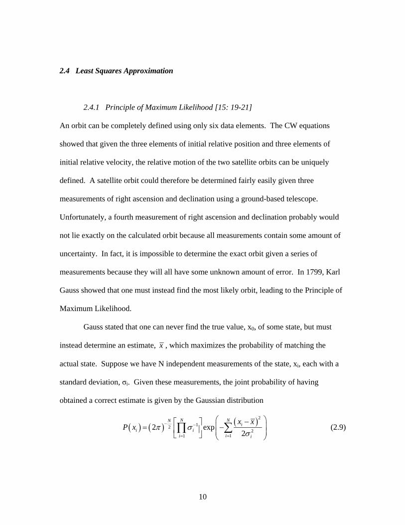
2.4.1 Principle of Maximum Likelihood [15: 19-21]
An orbit can be completely defined using only six data elements. The CW equations
showed that given the three elements of initial relative position and three elements of
initial relative velocity, the relative motion of the two satellite orbits can be uniquely
defined. A satellite orbit could therefore be determined fairly easily given three
measurements of right ascension and declination using a ground-based telescope.
Unfortunately, a fourth measurement of right ascension and declination probably would
not lie exactly on the calculated orbit because all measurements contain some amount of
uncertainty. In fact, it is impossible to determine the exact orbit given a series of
measurements because they will all have some unknown amount of error. In 1799, Karl
Gauss showed that one must instead find the most likely orbit, leading to the Principle of
Maximum Likelihood.
Gauss stated that one can never find the true value, x0, of some state, but must
instead determine an estimate, x , which maximizes the probability of matching the
actual state. Suppose we have N independent measurements of the state, xi, each with a
standard deviation, σi. Given these measurements, the joint probability of having
obtained a correct estimate is given by the Gaussian distribution
( ) ( ) ( )212
211
2 exp2
N NNi
i iii i
x xP x π σ
σ− −
==
⎛ ⎞−⎡ ⎤= −⎜⎢ ⎥ ⎜⎣ ⎦ ⎝ ⎠
∑∏ ⎟⎟
(2.9)
10

We can then find the best estimate, x , by maximizing this probability distribution. This
is done by minimizing the exponent, or solving the following equation:
( )2
21
02
Ni
i i
x xddx σ=
−=∑ (2.10)
Minimizing the squared term in the exponent gives the procedure its name: Method of
Least Squares.
2.4.2 Linear Least Squares [14: 67-70]
The method of linear least squares uses a series of observations, zi, to estimate the state,
x, of a system. We begin with knowledge of the state dynamics:
( ) ( ) ( )0 0,x t t t x t= Φ (2.11)
Linear least squares gets its name because we assume the observations are linearly related
to the system state by the following formula:
( ) ( )i i i i iz t H x t e= + (2.12)
where Hi is a matrix relating the observations, z, to the state, x, and ei is the unknown
error in the observations. Recalling from Eq. (2.11) that the state at any time can be
written in terms of the initial state, we can rewrite Eq. (2.12) as
( ) ( )0i i i iz t T x t e= + (2.13)
where = . The final necessary input is the covariance, QiT iH Φ i, of each observation.
This is a property of the observing instrument that gives an indication of the instrument’s
level of precision. If the set of observations was taken with multiple instruments, the
covariances will serve to give more weight to the observations taken with the more
precise instruments.
11

It is common to assemble the required information as follows:
1
2
N
zz
z
z
⎛ ⎞⎜ ⎟⎜ ⎟≡⎜ ⎟⎜ ⎟⎝ ⎠
(2.14)
( )( )
( )
1 1 0
2 2 0
0
,,
,N N
H t tH t t
T
H t t
Φ⎛ ⎞⎜ ⎟Φ⎜≡ ⎜⎜ ⎟⎜ ⎟Φ⎝ ⎠
⎟⎟
⎟⎟
(2.15)
1
2
0 00 0
0 0 N
Q
Q
⎛ ⎞⎜ ⎟⎜≡⎜⎜ ⎟⎝ ⎠
……
…
(2.16)
We can then calculate the covariance of the estimated state:
( ) 11TxP T Q T
−−= (2.17)
Finally, the estimated state is given by
( ) ( )10
Txx t P T Q z−= (2.18)
2.4.3 Nonlinear Least Squares [15: 74-81]
In many cases, including the subject of this thesis, the relationship between the
observations and the state being estimated is not linear. These nonlinear cases require a
different method of solution. Rather than simply solving for the estimated state, we must
make a guess at some reference state, refx , determine how well the observations match
12
this reference state, and calculate a correction, xδ , to the reference state. We then add
this correction to the reference state and iterate until we believe the reference state has
converged on the true state.
We begin with the assumption that variations in the system dynamics are linear,
or can at least be approximated by a linear function. Additionally, any correction to the
initial state can also be linearly propagated in time:
( ) ( ) ( )0, 0x t t t x tδ = Φ δ (2.19)
We can write the nonlinear observation relation as follows:
( ) ( )( ),i i i iz t G x t t= (2.20)
The observation relation can be linearized by solving for the error in the observations.
Recall that a perfect instrument would make a perfect observation, , of the true state, 0z
0x . A real instrument, however, will observe imperfect data, , resulting from an
imperfectly observed state,
z
x . The instrument error is then given by
( ) ( )( ) ( )
( )
0
0
0
, ,
,
e z zG x t G x t
G x x t G x tG x tx
δ
δ
0 ,
= −
= −
= + −
∂≈∂
(2.21)
Keeping a similar form to linear least squares, we can rewrite this as
( ) ( )( ,i i ref i iG )H t x t tx
∂≡∂
(2.22)
where is the linearized observation relation. The estimated reference state can be
compared to the observations by calculating the residual:
iH
( )( ),i i ref i ir z G x t t= − (2.23)
13

The residuals therefore give an indication of how close the reference state is to the true
observed state, and the goal of this process is to minimize the residuals by applying
corrections to the reference state. In fact, the residuals are related to the state correction
as follows:
( )( ) (( )
0
0
,i i i
i i
i
r H x t
H t t x t
T x t
δ
δ
δ
≈
= Φ
=
)0 (2.24)
Determining the state correction now becomes very similar to the method used in linear
least squares. The covariance of the correction is given by
11T
x i i ii
P T Q Tδ
−−⎛= ⎜
⎝ ⎠∑ ⎞
⎟ (2.25)
and the state correction is
( ) 10
Tx i i i
ix t P T Qδδ −= r∑ (2.26)
The reference state is then improved by adding the correction factor:
( ) ( ) ( )1 0 0 0ref refx t x t x tδ+ = + (2.27)
This process is then iterated until the reference state converges to a solution, where the
degree of convergence is determined by the size of the residuals.
14

III. Methodology
This chapter will discuss the methods of solution used to detect geostationary
satellite maneuvers. It will begin with an explanation of the reference frame and
observation geometry used, also describing how the equations of motion were applied.
Explanations of both the theory and computer algorithm used to model the motion of a
non-maneuvering satellite will follow. Finally, the methods used to detect maneuvers
and estimate the resulting satellite motion will be discussed.
3.1 Determining Observation Geometry
3.1.1 Application of Clohessy-Wiltshire Equations
The Clohessy-Wiltshire (CW) equations as shown in Eqs. 2.3 - 2.8 give the relative
motion between two satellites. For the purposes of this research, however, only one
satellite is considered. The CW equations are therefore applied to the relative motion
between the satellite of interest and an imaginary reference satellite. This reference
satellite is considered to be perfectly stationary at 0º latitude and the desired longitude of
the real satellite. Thus, the reference satellite represents the ideal location of the real
satellite, and the relative separation represents the deviation from its ideal location.
15

Following Eqs. 2.1 and 2.2, the system state will be given as
0
0
rr
zx
rr
z
δδθδδδθδ
⎛ ⎞⎜ ⎟⎜ ⎟⎜ ⎟
= ⎜⎜ ⎟⎜ ⎟⎜ ⎟⎜ ⎟⎝ ⎠
⎟ (3.1)
The state transition matrix then becomes a 6x6 combination of the CW matrices in Eqs.
2.5 – 2.8.
rr rv
vr vv
Φ Φ⎡ ⎤Φ = ⎢ ⎥Φ Φ⎣ ⎦
(3.2)
The use of an ideal reference satellite allows for further simplifications to be
made. Since both the observing station and the reference satellite rotate with the earth at
the exact same rate, this rotation can be ignored. The problem can be set up in the earth
centered-earth fixed (ECEF) frame, rather than the earth centered inertial (ECI) frame.
This allows the time-varying angle between the vernal equinox and Earth’s 0º longitude
to be ignored. Although this simplifies the observation equations, it actually causes the
right ascension angle to be incorrectly defined. Right ascension is referenced to the
vernal equinox, while the angle referred to as right ascension in this research is
referenced to the local meridian of the observing site. For simplicity, however, the term
right ascension will still be used.
3.1.2 Observations to State Conversion
The system state is given in terms of the relative separation between the satellite of
interest and a reference satellite in an ideal orbit. The observations, however, are given
16

as right ascension (α) and declination (δ) from the point of view of the observing site.
The conversion from the observations to the state must take into account the position of
both the observing site and the satellite in the ECEF reference frame.
Figure 3.1: Observation Geometry
Following Figure 3.1, the position of the satellite in the ECEF frame is given as
( ) ( )( ) (
cos
sin
ref ref
ref ref
R rxr y R r
z z)
δ λ δθ
δ λ δθ
δ
⎛ ⎞+ +⎛ ⎞ ⎜ ⎟⎜ ⎟ ⎜= = + +⎜ ⎟ ⎜ ⎟⎜ ⎟ ⎜ ⎟⎝ ⎠
⎝ ⎠
⎟ (3.3)
17

where refR is the radius of the reference satellite’s orbit, refλ gives the longitude of the
reference satellite, and rδ , δθ , and zδ are the relative separation components of the
system state. The position of the observing site in the ECEF frame is given by the
following equation.
cos coscos sin
sin
e
e
e
X RY RZ R
φ λφ λφ
⎛ ⎞ ⎛ ⎞⎜ ⎟ ⎜ ⎟=⎜ ⎟ ⎜ ⎟⎜ ⎟ ⎜ ⎟⎝ ⎠ ⎝ ⎠
(3.4)
eR is the radius of the earth, φ denotes the latitude of the observing site, and λ denotes
the longitude of the observing site. The observation vector, made up of right ascension
and declination, is determined by
( ) ( )2 2
arctan
arctan
y Yx X
zz Z
x X y Y
αδ
⎛ −⎛ ⎞⎜ ⎟⎜ ⎟−⎝ ⎠⎜ ⎟⎛ ⎞
= = ⎜ ⎟⎜ ⎟ ⎛ −⎝ ⎠ ⎜ ⎟⎜ ⎟⎜ ⎟⎜ ⎟⎜ ⎟− + −⎝ ⎠⎝ ⎠
⎞
⎞ (3.5)
Substituting Eqs. 3.3 and 3.4 into Eq. 3.5 will give right ascension and declination in
terms of the relative separation variables of the system state. Since Eq. 3.5 relates the
observation variable to the state variables, it is known as the observation relation, denoted
as G from Eq. 2.20. For the purposes of nonlinear least squares (NLS) estimation, this
observation relation must be linearized. This is done by taking partial derivatives of both
elements of the observation relation with respect to each element of the state. Following
Eq. 2.22, the resulting linearized observation relation is given by
0 0
0 0
r r z r r zzHx
r r z r r z
α α α α α αδ δθ δ δ δθ δδ δ δ δ δ δδ δθ δ δ δθ δ
∂ ∂ ∂ ∂ ∂ ∂⎡ ⎤⎢ ⎥∂ ∂ ∂ ∂ ∂ ∂∂ ⎢ ⎥= =∂ ∂ ∂ ∂ ∂ ∂⎢ ⎥∂
⎢ ⎥∂ ∂ ∂ ∂ ∂ ∂⎣ ⎦
(3.6)
18

The six partial derivatives with respect to the velocity terms of the state will be zero,
since no velocity components appear in Eq. 3.5. The other six derivatives in the left half
of the H matrix, however, result in large equations that were solved by hand and
confirmed using Maple V by Waterloo Maple, Inc. Those equations are derived and
shown in Appendix A.
3.2 Test Data Generator
3.2.1 Non-maneuver Test Data
A method of creating test data was made as a means to check the accuracy of the orbit
determination models. This allows the initial state, maneuver time, and maneuver vector
to be pre-determined, giving a standard against which the model’s results can be
compared. The first step in generating test data was to choose an initial state. This initial
state can be hard coded in order to provide a known true state to compare against, or it
can be created using a random number generator to simulate data with an unknown initial
position and trajectory. A time vector spanning ten days was chosen, and the initial state
was propagated over the time vector using the state transition matrix from Eq. 3.2. At
this point, the option was available to add a small random component to each element of
the state for each timestep. This simulates the uncertainty inherent in real observations.
For each time element, the state vector was then converted into right ascension and
declination following the observation geometry described in Section 3.1.2.
19

Figure 3.2: Sample of Non-maneuver Test Data
20

Figure 3.2 shows an example of data produced from the test data generator.
Figure (a) plots declination with respect to right ascension, showing how the satellite’s
motion would appear as seen from the ground. Figures (b) and (c) plot the right
ascension and declination, respectively, as a function of time. It is apparent that both
right ascension and declination oscillate with a period of one day, and a drift in the East-
West direction causes the right ascension to steadily decrease.
Contrary to what is shown in Figure 3.2, real observation data would not be
continuous over the course of several days. Optical observations can only be taken at
night, and tight observing schedules generally result in, at most, an observing time of a
couple hours for each object of interest. In order to incorporate this into the test data
generator, the time vector was truncated in order to only include a few observations each
night. In fact, the time vector was restructured as a collection of two hour spans divided
into five minute intervals. A 22 hour dead time was included between each two hour
span. This resulted in a more accurate simulation of real observation data. An example
is shown in Figure 3.3. Although not obvious from simple observation, the orbit shown
in Figure 3.3 is exactly the same as the one in Figure 3.2. Appendix B shows the
MATLAB code for the non-maneuver test data generator.
21

Figure 3.3: Sample of Truncated Non-maneuver Test Data
22

3.2.1 Maneuver Test Data
A similar approach was used for the creation of test data in which a maneuver is
included. After propagating the initial state vector over the time span of interest, a
particular time point was chosen to be the maneuver time. The selection of the maneuver
time could either be user defined or chosen by a random number generator. In either
case, the time of maneuver was stored as an output variable in order to provide a standard
to compare the maneuver model against.
In order to create the maneuver, the system state at the chosen maneuver time was
adjusted. Most stationkeeping maneuvers occur in either the North-South direction or the
East-West direction [10: 343]. In terms of the system state, as shown in Eq. 3.1, a North-
South maneuver corresponded to an adjustment to the zδ term, while an East-West
maneuver corresponded to a change in the 0r δθ term. Having adjusted the system state
at the time of the maneuver, it was then considered to be the initial state for all post-
maneuver states propagated for the remainder of the time vector. The states were finally
converted into right ascensions and declinations following the same method used for the
non-maneuver data generator. Appendix C shows the code that generates the maneuver
test data. Figure 3.4 shows an example of a continuous set of maneuver data, while
Figure 3.5 shows the same data set truncated into nightly observing sessions. Notice that
the maneuver is most evident in the right ascension plot, indicating that the maneuver is
an East-West maneuver in this case.
23
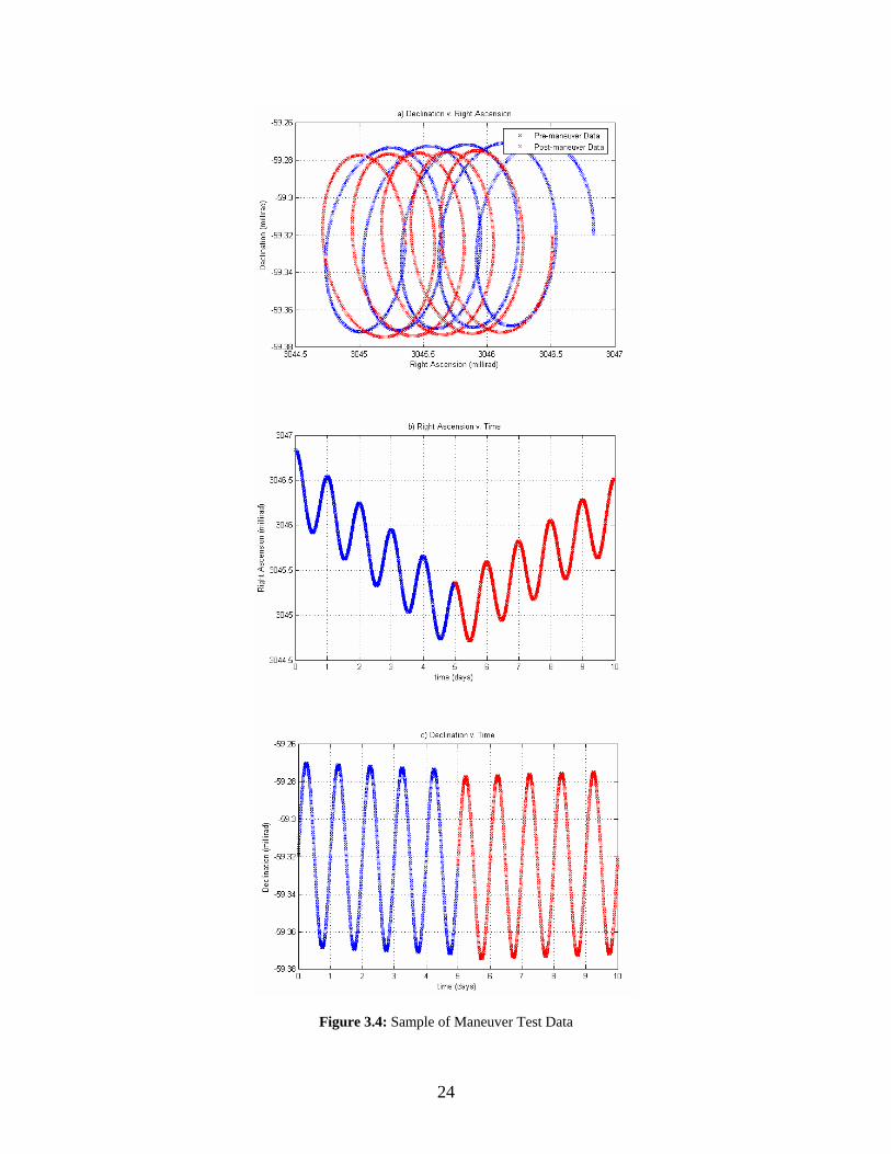
Figure 3.4: Sample of Maneuver Test Data
24

Figure 3.5: Sample of Truncated Maneuver Test Data
25

3.3 Non-maneuver Model
Before attempting to estimate maneuvers, a non-maneuver model was created that
would use the nonlinear least squares process to estimate a satellite’s orbit given
observed non-maneuver data. The provided data is in the form of an obscard file which
gives the right ascension, declination, and date of a series of observations. Using a
modified version of a MATLAB program written by Keric Hill while working at AMOS
in the summer of 2003, the obscard file is converted to right ascension, declination, and
time vectors. Recall from Section 2.4.3 that the nonlinear least squares method requires
an initial guess of the system’s initial state. Since there is no a priori information as to
the satellite’s actual initial position, the initial guess is the zero vector. This means the
algorithm initially assumes there is no relative separation or relative velocity between the
actual satellite and the reference satellite. Another user input is the covariance of the
observation vector, denoted as Q in Eq. 2.16. The entries of this matrix signify the
accuracy of the observing telescope. For this research, the telescope used had both a
right ascension and declination covariance of one square arcsecond, as provided by
operators at AMOS.
Having defined all necessary input, the following gives a summary of the
nonlinear least squares algorithm as applied to the non-maneuver data. For each
observation, the initial guess of the system’s initial state is propagated to the observation
time using the state transition matrix, Φ, as defined by Eq. 3.2. The observation relation
and linearized observation relation are both determined for each state vector using
26

Eqs. 3.3 – 3.6. Following Eq. 2.23, the residual is calculated. Finally, the following two
running sums are updated for each observation:
1Ti i i
i
T Q T−∑ (3.7)
1Ti i i
i
T Q r−∑ (3.8)
Q is the covariance defined in Eq. 2.16, = iT iH Φ , and r is the residual defined by Eq.
2.23. Once each observation is considered and the two running sums are updated, the
state correction and its covariance are determined following Eqs. 2.25 and 2.26. The
state correction term is then used to update the guess of the initial state as shown in Eq.
2.27, and the process is iterated until the guess of the initial state converges to the true
initial state. Convergence is generally confirmed by observing the residuals and ensuring
they are sufficiently small. The covariance of the observations can be used as a metric to
define when the residuals are small enough. There is no reason to continue iterations
when the residuals become smaller than the uncertainty in the measurements. Once the
initial state is found, it can be propagated over any time vector of choice in order to
determine the satellite’s orbit over that time vector. This program is shown in its entirety
in Appendix D.
3.4 Maneuver Model
The first step in the algorithm to model the orbit of a maneuvering satellite is to
separate the data into pre-maneuver and post-maneuver segments. It is assumed that only
one maneuver takes place during the time span of observations. As the observation data
27

is processed, it should become apparent from visual inspection if multiple maneuvers
occurred during a given data set. The data could then simply be separated such that only
one maneuver is contained in each set. An additional assumption is that the data will be
arranged in nightly observing sessions, similar to what is shown in Figure 3.5, and that
the maneuver takes place at some time after the first observing session.
3.4.1 Separating Data with an East-West Maneuver
With these assumptions in mind, the algorithm pulls out the first observing session and
fits a nonlinear least squares curve using only this first clump of data. Propagating this
estimation over the entire data set should result in a curve that fits the pre-maneuver data
set fairly well, but diverges from the post-maneuver data, as shown in Figure 3.6. Notice
once again that in this example, an East-West maneuver took place, evident by the
obvious change in the right ascension trend. By converting the fitted curve into discrete
points that match up with the data points, as shown in Figure 3.7, a simple subtraction
can be made.
If the uncertainty in the observations is large enough, the first clump of data may
not be enough to fit a nonlinear least squares curve that closely approximates all the pre-
maneuver observations. In cases such as these where more data points are needed to
produce an accurate initial fit, the algorithm allows for both the first and second
observation data clumps to be used. While more data points should always increase the
accuracy of the initial pre-maneuver fit, including the second data clump introduces the
constraint that the maneuver cannot occur between the first and second observing
sessions.
28

Figure 3.6: NLS curve fitted to first data set
29

Figure 3.7: Discrete NLS curve fitted to first data set
30

The difference between the nonlinear least squares fit and the observed data
points are plotted in Figure 3.8. Recall that the difference is most noticeable in the right
ascension difference because the simulated maneuver is in the East-West direction. Had
the maneuver been in the North-South direction, the change would have been evident in
the declination difference.
Figure 3.8: Difference between NLS Fit and Observed Data for an E-W maneuver
By visual inspection, it is clear from Figure 3.8 that a maneuver occurred at some
time between the data set at Day 5 and the data set at Day 6. Unfortunately, designing an
algorithm so a computer can determine the approximate maneuver time is a bit more
complicated. As the magnitude of the maneuver will directly affect the scale of the angle
differences, the right ascension difference was first scaled according to the largest data
point, as shown in Figure 3.9.
31

Figure 3.9: Scaled Difference between NLS Fit and Observed Data
It would seem reasonable to simply define some cutoff difference such that the
maneuver is determined to occur once the difference exceeds this cutoff difference.
However, this would not be a feasible method in cases where the maneuver took place
during one of the observing sessions. As most stationkeeping maneuvers take place at
night when the satellite is less likely to be in use, this is a valid concern. Notice that
before the maneuver, the slope of the curve is approximately zero, while the slope as
some positive value after the maneuver. The absolute value of the slope between each of
the scaled difference data points from Figure 3.9 was therefore calculated. Figure 3.10
shows the result of this slope calculation.
32

Figure 3.10: Slope between the Data Points from Figure 3.9
Once again, it is visually apparent that the maneuver takes place sometime
between the fifth and sixth day. As expected from Figure 3.9, the slopes of the pre-
maneuver data are all very close to zero, while the post-maneuver data have relatively
larger slopes. Next, the percentage difference between the slope data of Figure 3.10 was
calculated by dividing the difference between two consecutive data points by the first of
the two data points. Figure 3.11 shows these percentage differences.
33

Figure 3.11: Percentage Difference between the Data Points from Figure 3.10
The percentage difference between the point just before the maneuver and the
point just after the maneuver is significantly larger than all other percentage differences
because it is the only one that has both the relatively large slope difference characteristic
to the post-maneuver data, while also containing a small pre-maneuver data point in the
denominator of the percentage difference calculation. Thus, the percentage difference
gives a clear indication of where to separate the data into pre-maneuver and post-
maneuver observations. Figure 3.12 shows a correct separation.
34

Figure 3.12: Observation Data Separated into Pre-maneuver and Post-maneuver Sets
35

3.4.2 Separating Data with a North-South Maneuver
The method used to separate the data when a North-South stationkeeping maneuver took
place is slightly different that the East-West method just described. Since there is no drift
in the declination, any North-South maneuver will simply change the amplitude and
possibly shift the phase of the sinusoidal declination curve. The period and average value
of the declination will remain the same.
Following the same method as in the East-West maneuver algorithm, a nonlinear
least squares curve is fitted to the first observing session. Notice in Figure 3.13 that in
the case of a North-South maneuver, the declination strays from the fitted curve after the
maneuver, while the right ascension remains fairly close to the NLS approximation. Once
again, the difference between the observed data and the NLS fitted data is plotted. As
seen in Figure 3.14, the declination difference curve clearly shows that the maneuver
took place sometime between the fifth and sixth day.
36

Figure 3.13: NLS curve fitted to first data set
37
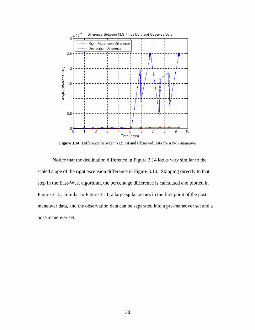
Figure 3.14: Difference between NLS Fit and Observed Data for a N-S maneuver
Notice that the declination difference in Figure 3.14 looks very similar to the
scaled slope of the right ascension difference in Figure 3.10. Skipping directly to that
step in the East-West algorithm, the percentage difference is calculated and plotted in
Figure 3.15. Similar to Figure 3.11, a large spike occurs in the first point of the post-
maneuver data, and the observation data can be separated into a pre-maneuver set and a
post-maneuver set.
38

Figure 3.15: Percentage Difference between the Data Points from Figure 3.14
Since the algorithm used to separate the data for an East-West maneuver is
different than for a North-South maneuver, some technique to determine beforehand
which type of maneuver occurs must be included. Referring back to Figures 3.8 and
3.14, these charts plot the right ascension and declination differences for each example
maneuver. For East-West maneuvers, the right ascension difference has a much greater
maximum value than the declination difference. Likewise, the declination difference has
a much greater maximum difference for North-South maneuvers. The type of maneuver
can therefore quickly be determined from the maximum difference.
39

3.4.3 Corrections to Data Separation Models
During the course of this research, it was found that the random error added to each
element of the generated test data was not large enough to provide an accurate
representation of the uncertainty inherent in real optical observations. Earth’s non-
homogenous atmosphere causes light from space to be randomly refracted, thus limiting
the resolution of any ground-based observations. At sea level, atmospheric effects
usually limit the resolution of optical observations to about one arcsecond. The Air Force
Maui Optical Station (AMOS), located at about 10,000 ft above sea level, can obtain
resolutions of one half to one quarter of an arcsecond on very clear nights [2: 159-169].
While the methods described in Sections 3.4.1 and 3.4.2 originally resulted in an
accurate separation of pre-maneuver and post-maneuver observations, they were found to
be inaccurate when more random noise was added to the observation data. The methods
above tended to amplify the noise to the extent that false maneuvers were occasionally
detected in data with uncertainties of one arcsecond or more. In response to this, the
methods used to separate the pre-maneuver and post-maneuver data for both East-West
and North-South maneuvers were slightly revised.
Errors in the method for East-West maneuvers stemmed from calculating the
slope of the right ascension difference plot, as shown in Figure 3.10. Data points in the
same observing session are often very close together chronologically, therefore noisy data
can result in relatively large slopes. Figure 3.16 shows how noise can affect the slope
calculation, turning the orderly plot in Figure 3.10 into an unintelligible mess.
40

Figure 3.16: Slope between the Data Points Using Noisy Data
Figure 3.17: Modified Slope between the Data Points Using Noisy Data
41

The effects of the noise in the data were minimized by modifying the slope
calculation. Rather than calculating the slope, a second difference of the scaled
difference was calculated. Thus, the rise over run calculation of the slope was discarded
for a simple rise calculation without dividing by the run. Referring back to Figure 3.9, it
can be seen that the largest differences occur between the nightly observing sessions after
the maneuver occurs. These will therefore show up as peaks in the second difference
calculation. Shown in Figure 3.17, the first point of each post-maneuver data clump,
marked by a blue circle, is greatly accented. The same points in Figure 3.16, also shown
as blue circles, were obscured by the noisy data. From Figure 3.17, the data can be easily
separated according to the first peak. A flow chart summarizing the data separation
method is shown in Figure 3.18.
Figure 3.18: Flow Chart of Data Separation Method for E-W Maneuver
Increased uncertainty in the observation data had a similar effect for North-South
maneuvers. The original method to separate pre-maneuver and post-maneuver data for a
North-South maneuver involved calculating a percentage difference. For pre-maneuver
data, the difference due to noise is significantly amplified as the percentage calculation
involves dividing by a very small number. This effect was neutralized by multiplying the
percentage by the second of the two data points. This effectively amplified the post-
maneuver percentages, while suppressing pre-maneuver percentages. Figure 3.20 shows
42

a percentage difference calculation, similar to Figure 3.15, in which noise is included.
Notice the actual separation point, shown by the blue circle, is dwarfed by pre-maneuver
peaks created by noise. Figure 3.21 shows the same data using the improved method of
multiplying by the second data point. Notice that all the post-maneuver peaks are
amplified, while the pre-maneuver noise is suppressed. The actual separation point is
once again the maximum value. A flow chart summarizing this revised method is shown
in Figure 3.19.
Figure 3.19: Flow Chart of Data Separation Method for N-S Maneuver
Figure 3.20: Percentage Difference between the Data Points Using Noisy Data
43

Figure 3.21: Modified Percentage Difference between the Data Points Using Noisy Data
3.4.4 Determining Possible Maneuver Times
Having separated the data into a pre-maneuver partition and a post-maneuver partition,
the nonlinear least squares algorithm can be applied to both sets separately. This will
result in two fitted curves that should intersect at the maneuver time, as shown in Figure
3.22. Assuming both NLS curves are fairly accurate representations of the actual path of
the satellite both before and after the maneuver, the two curves should intersect at the
actual maneuver time.
44

Figure 3.22: Sample of Pre-maneuver and Post-maneuver NLS Fits
45

Figure 3.23 shows a close up of the region surrounding the intersection point for
the East-West maneuver from Figure 3.22. Notice that there are multiple points where
the two nonlinear least squares curves intersect. Since both right ascension and
declination follow sinusoidal curves, there will almost always be multiple intersections
between the pre-maneuver curve and the post-maneuver curve. Each intersection
corresponds to a possible maneuver and time of maneuver that would transfer the satellite
from its pre-maneuver trajectory to its post-maneuver trajectory.
Figure 3.23: Close-up of NLS Fits Showing Possible Maneuver Intersections
In order to locate all the intersections, the difference between the post-maneuver
and pre-maneuver fits is calculated. Shown in Figure 3.24, the intersections occur where
the difference equals zero. Unfortunately, these fits are not continuous lines, but are
rather made up of discrete points. It is therefore extremely unlikely that the difference
will ever equal zero; it will instead contain minima at the intersection times. Figure 3.25
gives a closer view of the intersection region of Figure 3.24.
46

Figure 3.24: Difference between Pre-maneuver and Post-maneuver Fits
Figure 3.25: Intersection Region of Pre-maneuver and Post-maneuver Difference Plot
47

Each minimum will most likely have a different value, so the data must be
separated into groups containing only one minimum. Otherwise, the algorithm will only
locate the smallest of the multiple minima. The first step in separating the minima
involves disregarding all difference data that is above some threshold value.
Notice the small humps between the intersection points in Figure 3.25. The size
of these humps depends upon the difference in the post-maneuver and pre-maneuver fits
between intersection points, as well as the angle between the fits at the intersection point.
It is therefore impossible to predict beforehand if the entire humps will fall under the
threshold value, or if only the regions surrounding the minima will be kept. Either way,
the minima will be characterized by having a set of data points with a negative slope to
the left of the minimum and a set of data points with a positive slope to the right of the
minimum. Separating the data at every point where the slope changes from positive to
negative will result in a split at the peaks of each hump. This will result in groups of data
containing one minimum per group, each designating a possible maneuver time.
3.4.5 Choosing Correct Maneuver Time
The method to determine which of these intersections corresponds to the real maneuver
draws upon the previously stated assumption that all stationkeeping maneuvers will be
either in the North-South direction or the East-West direction. At each intersection, the
velocity components of the system state are extracted from the pre-maneuver NLS fit and
the post-maneuver NLS fit. The difference between each of the three velocity
components defines the three-dimensional maneuver.
48

Using the notation for the velocity components of the system state defined in Eq.
3.1, the maneuver is calculated for each intersection point using the following formula.
( )( )( )
( ) ( )
( ) ( )( ) ( )
0 0 0
post maneuver pre maneuver
post maneuver pre maneuver
post maneuver pre maneuver
r rr
maneuver r r r
z z z
δ δδ
δθ δθ δθ
δ δ δ
− −
− −
− −
⎛ ⎞−⎛ ⎞Δ ⎜ ⎟⎜ ⎟⎜ ⎟= Δ = −⎜ ⎟⎜ ⎟⎜ ⎟⎜ ⎟ ⎜ ⎟Δ −⎝ ⎠ ⎝ ⎠
(3.9)
From the perspective of a ground station, rδ describes the radial velocity, 0r δθ defines
the velocity in the East-West direction, and zδ gives the velocity in the North-South
direction. How closely each maneuver approximates a purely East-West or North-South
maneuver is determined by calculating what percentage of the maneuver vector is in the
0r δθ term or the zδ term, respectively.
( )( ) ( ) ( )
0
22 20
%E W
r
r r z
δθ
δ δθ δ−
Δ=
Δ + Δ + Δ (3.10)
( )( ) ( ) ( )
22 20
%N S
z
r r z
δ
δ δθ δ−
Δ=
Δ + Δ + Δ (3.11)
Eq. 3.10 identifies what percentage of the maneuver is in the East-West direction, while
Eq. 3.11 describes what percentage is in the North-South direction. The correct
maneuver can therefore be determined by creating a simple algorithm that simultaneously
searches through both percentages for each possible maneuver to find a maximum. The
maneuver in which this maximum occurs is determined to be the correct maneuver.
49

3.4.6 Non-maneuver Data in the Maneuver Model
In addition to determining the maneuver vector and time of maneuver, a robust maneuver
detection model must also be able to recognize when no maneuver took place. If an
observation data set that contains no maneuver is fed into the previously described
maneuver model, the algorithm will first attempt to separate the data into a pre-maneuver
segment and a post-maneuver segment. Although there will be no clearly defined
maneuver peak as in Figures 3.11 or 3.15, the model will find a peak and separate the
data accordingly. The pre-maneuver and post-maneuver NLS fits will align very closely,
but the algorithm will still determine a maneuver and maneuver time.
Experimental analysis using several sample non-maneuver data sets showed that
the determined maneuver was generally on the order of 10 nm/s. A threshold maneuver
magnitude of 1 mm/s was therefore included. If the detected maneuver is below 1 mm/s,
the algorithm will advise the user to apply that data set to the non-maneuver model.
50

IV. Simulation Results
This chapter will summarize the results of the simulation in response to various
types of observation data. The first section will focus on data containing a maneuver in
the East-West direction. The minimum detectable maneuver size will be addressed, as
well as the model’s response to data with varying degrees of uncertainty. The section
will also review the model’s ability to detect a maneuver that occurs during an observing
session and maneuvers that occur near the beginning or end of a particular data set. The
second section will discuss these aspects with respect to North-South maneuvers. The
differences in the response to these maneuvers will be addressed, as well as their
implications.
4.1 Response to East-West Maneuvers
4.1.1 Response to Ideal Data
Initial test data, representing best possible seeing conditions, was generated with a
simulated uncertainty of ±0.2 arcseconds. For the first test case, data was generated
containing a 3 cm/s maneuver at a time of 5.5 days. Figure 4.1 shows the observation
data, along with an initial non-maneuver NLS fit. The algorithm detected the maneuver,
determining it to occur at 5.49 days, with a magnitude of 3.02 cm/s. Figure 4.2 shows the
resulting estimation of the satellite’s pre-maneuver and post-maneuver trajectory.
51

Figure 4.1: Test Data with 3 cm/s E-W Maneuver at 5.5 days
52

Figure 4.2: Response to Test Data from Figure 4.1
53
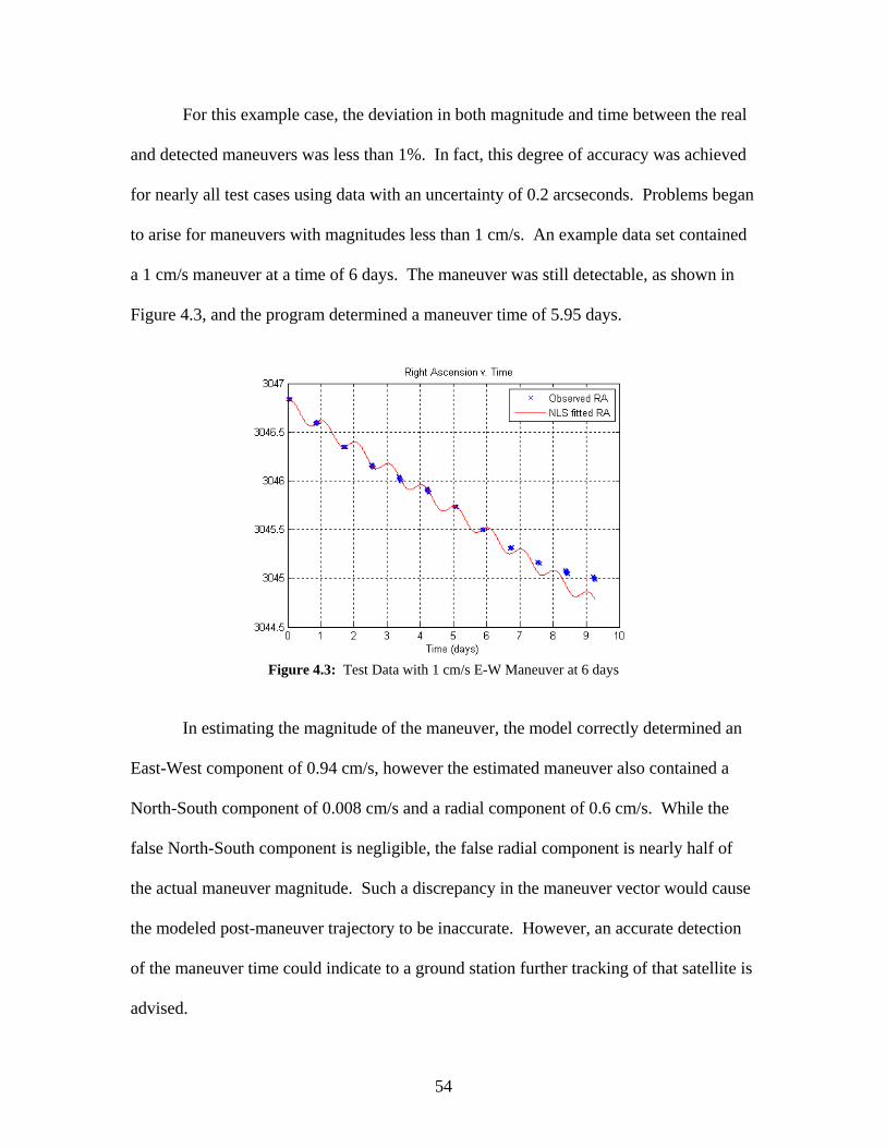
For this example case, the deviation in both magnitude and time between the real
and detected maneuvers was less than 1%. In fact, this degree of accuracy was achieved
for nearly all test cases using data with an uncertainty of 0.2 arcseconds. Problems began
to arise for maneuvers with magnitudes less than 1 cm/s. An example data set contained
a 1 cm/s maneuver at a time of 6 days. The maneuver was still detectable, as shown in
Figure 4.3, and the program determined a maneuver time of 5.95 days.
Figure 4.3: Test Data with 1 cm/s E-W Maneuver at 6 days
In estimating the magnitude of the maneuver, the model correctly determined an
East-West component of 0.94 cm/s, however the estimated maneuver also contained a
North-South component of 0.008 cm/s and a radial component of 0.6 cm/s. While the
false North-South component is negligible, the false radial component is nearly half of
the actual maneuver magnitude. Such a discrepancy in the maneuver vector would cause
the modeled post-maneuver trajectory to be inaccurate. However, an accurate detection
of the maneuver time could indicate to a ground station further tracking of that satellite is
advised.
54

4.1.2 Response to Increasingly Uncertain Data
While an observation uncertainty of 0.2 arcseconds is theoretically achievable on very
clear nights at observing stations at high altitudes, a more reasonable uncertainty of one
arcsecond was analyzed next. When given data with this degree of uncertainty, the
model is no longer able to accurately separate the pre-maneuver and post-maneuver data
for small maneuvers. As an example, observation data was generated with a 1.5 cm/s
maneuver occuring at a time of 6 days. The data was randomly adjusted in order to
simulate an uncertainty of one arcsecond. Such a small maneuver with respect to the
amount of uncertainty in the observations resulted in the model incorrectly separating the
pre-maneuver and post-maneuver data in the middle of the observation cluster centered
on about 1.7 days, as shown in Figure 4.4. Figure 4.5 shows the resulting incorrect
trajectory fit. Notice that the noise in the data seems more prevalent in the declination
plot. This will be discussed further in the next example.
Figure 4.4: Incorrect separation for 1.5 cm/s Maneuver at 6 days
55

Figure 4.5: Incorrect Estimated Trajectory for 1.5 cm/s Maneuver at 6 days
56

It was determined that for data with a 1 arcsecond uncertainty, the minimum
detectible East-West maneuver had a magnitude of about 5.5 cm/s. Decreasing the
maneuver magnitude further resulted in the model occasionally misidentifying the correct
pre-maneuver/post-maneuver separation point. When the maneuver time was correctly
estimated, the maneuver vector often contained significant components in the North-
South and radial directions, similar to the case described earlier.
The uncertainty in the test data was further increased to 2 arcseconds. For this
case it was found that increasing the uncertainty in the data did not significantly change
the minimum maneuver magnitude at which point the model could estimate the time of
maneuver. The model’s ability to estimate the magnitude and direction of the maneuver,
however, rapidly diminished.
Figure 4.6 shows the resulting analysis of data generated with an uncertainty of 2
arcseconds, containing an East-West maneuver of 4.25 cm/s at 6 days. While the model
successfully estimated the maneuver occurred at 5.97 days, the maneuver vector was
determined to be 3.1 cm/s in the East-West direction, 0.06 cm/s in the North-South
direction, and 2.24 cm/s in the radial direction.
Notice in Figure 4.6 that the right ascension plot looks fairly neat, while the
declination plot is a mess. This is due to the scaling of the graphs. While East-West drift
causes the right ascension to vary by about 1.4 milliradians, the declination only varies by
about 60 microradians. An uncertainty of 2 arcseconds corresponds to almost 10
microradians. While this is still fairly insignificant for the right ascension plot, it is over
30% of the declination curve’s amplitude. For this reason, the declination data is
practically useless when using data at this level of uncertainty.
57

Figure 4.6: Model’s Response to Data with 2 Arcsecond Uncertainty
58

4.1.3 Limits on Maneuver Time
This section investigates how the model responds to maneuvers that occur near the very
beginning or very end of the observation data set. In the first case, data was generated in
which the maneuver occurred just before the last clump of observations. In particular, the
data contained a 7 cm/s maneuver at 8.5 days. Figure 4.7 clearly shows that only the last
clump of data belongs in the post-maneuver set.
Figure 4.7: Test Data with 7 cm/s E-W Maneuver at 8.5 days
While the algorithm had no trouble separating the pre-maneuver and post-
maneuver data, fitting an NLS curve to the post-maneuver data proved difficult. As
Figure 4.8 shows, one clump of data is not enough to produce an accurate NLS fit. As
expected, such an inaccurate post-maneuver fit results in an incorrect estimate of both
maneuver time and vector.
59
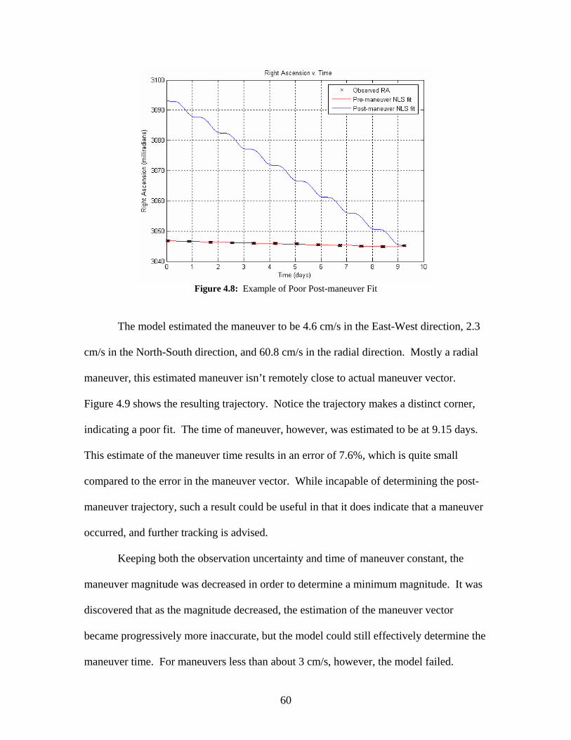
Figure 4.8: Example of Poor Post-maneuver Fit
The model estimated the maneuver to be 4.6 cm/s in the East-West direction, 2.3
cm/s in the North-South direction, and 60.8 cm/s in the radial direction. Mostly a radial
maneuver, this estimated maneuver isn’t remotely close to actual maneuver vector.
Figure 4.9 shows the resulting trajectory. Notice the trajectory makes a distinct corner,
indicating a poor fit. The time of maneuver, however, was estimated to be at 9.15 days.
This estimate of the maneuver time results in an error of 7.6%, which is quite small
compared to the error in the maneuver vector. While incapable of determining the post-
maneuver trajectory, such a result could be useful in that it does indicate that a maneuver
occurred, and further tracking is advised.
Keeping both the observation uncertainty and time of maneuver constant, the
maneuver magnitude was decreased in order to determine a minimum magnitude. It was
discovered that as the magnitude decreased, the estimation of the maneuver vector
became progressively more inaccurate, but the model could still effectively determine the
maneuver time. For maneuvers less than about 3 cm/s, however, the model failed.
60

Figure 4.9: Estimated Trajectory of Poor Post-maneuver Fit
Similar results occurred for maneuvers which occurred just before the second to
last clump of observations. Figure 4.10 shows that in these cases, the model could more
accurately fit an NLS curve to the post-maneuver data. While the estimated maneuver
vector was still very inaccurate, this did result in an even better estimate of maneuver
time than the cases in which only one clump of data was recorded after the maneuver.
Figure 4.10: Separation of Data with a Late Maneuver
61

Responses to maneuvers which occurred near the beginning of the observation
data proved to be slightly more accurate than responses to maneuvers occurring near the
end of the data set. As an example, data with a 3 cm/s maneuver at 1.2 days was
considered. This occurs just after the second clump of data. Just as before, the model
had no trouble determining the time of maneuver. It was estimated to occur at 1.15 days.
The maneuver magnitude was still somewhat inaccurate, with an estimated value of
4.41 cm/s. Figure 4.11 shows the resulting trajectory determined for that example.
Figure 4.11: Estimated Trajectory for 3 cm/s Maneuver at 1.2 days
Recall from Section 3.4.1 that the initial non-maneuver NLS fit used to determine
the pre-maneuver and post-maneuver separation point originally was formed by fitting a
curve to only the first clump of data. It was determined that noise in the observations
caused this initial fit to be inaccurate, so the first two observation clumps were instead
used to determine the initial fit. This requires the assumption that no maneuvers occur
between the first and second data clumps. For this reason, the model breaks down when
62

given data in which such a maneuver occurs. Reverting back to the use of only the first
data clump in the initial fit resulted in poor approximations when the data had an
uncertainty of 0.5 arcseconds or more. It was therefore determined that this model cannot
effectively detect a maneuver which occurs after only one observing session.
4.2 Response to North-South Maneuvers
Since there is no drift in the North-South direction, these maneuvers are
inherently more difficult to detect. Consider the North-South maneuver shown in Figure
4.12. This 7 cm/s maneuver occurred at 6 days and had a simulated uncertainty of 0.2
arcseconds. The pre-maneuver and post-maneuver data was accurately separated, as
shown in Figure 4.13, and NLS curves were fitted to both data sets.
Figure 4.12: Test Data with 7 cm/s N-S Maneuver at 6 days
63

Figure 4.13: Separation of Test Data with 7 cm/s N-S Maneuver at 6 days
Notice that a North-South maneuver appears as an amplitude change in the
declination curve. Both the period and phase of the sinusoidal curve remain the same.
Because of this, each periodic intersection of the pre-maneuver and post-maneuver data
corresponds to an identical maneuver.
Recall from Section 3.4.5 that the correct maneuver time is determined by finding
which of the intersections corresponds to a maneuver that most closely matches an
entirely North-South maneuver or an entirely East-West maneuver. If every possible
maneuver is identical, there is no way to resolve which is the correct one. By
constraining the list of possible maneuvers to those that lie near the pre-maneuver/post-
maneuver separation point, the algorithm will usually end up randomly choosing either
the correct maneuver time or one of the two neighboring possible maneuvers.
In cases where sessions of observation data are gathered each night, this results in
an uncertainty in the estimated maneuver time of about 12 hours, as the intersections
64

between pre-maneuver and post-maneuver NLS fits occur every 12 hours. If there are
gaps in the data due to bad weather, there may be several more intersections between the
last pre-maneuver data point and the first post-maneuver data point. It will be impossible
to distinguish which of these intersections is the correct maneuver time, thus the potential
error in the maneuver time estimate will grow larger.
Figure 4.14 shows the model successfully estimating the maneuver to be 7.01
cm/s, occurring at a time of 6 days. Running the simulation multiple times showed that
the model would often incorrectly estimate that the maneuver occurred at 6.5 days.
According to Figure 4.13, this is the other intersection that occurs between the pre-
maneuver and post-maneuver data.
Figure 4.14: Estimated Trajectory of Test Data with 7 cm/s N-S Maneuver at 6 days
65

When a North-South maneuver occurs during an observing session, the model is
actually more likely to determine the correct maneuver time. Consider the 7 cm/s
maneuver at 5.1 days, as shown in Figure 4.15. While the example in Figure 4.13
showed two possible intersections that occured between the pre-maneuver and post-
maneuver data, this example has only one as the data is separated inside an observing
session.
Figure 4.15: Estimated Trajectory of Test Data with 7 cm/s N-S Maneuver at 5.1 days
4.2.1 Response to Uncertain Data
Since the variation of the declination curve occurs on such a small scale, increasing the
uncertainty in the observation data has a much larger effect on detecting North-South
maneuvers. Figure 4.16 shows a 10 cm/s maneuver at 5.1 days with an uncertainty of 1
arcsecond.
66

Figure 4.16: Example of Correct Fit to Data with 1 arcsecond Uncertainty
67

While Figure 4.16 shows a case in which the maneuver time and vector was
correctly estimated, this was an exception to the trend of difficulties in detecting North-
South maneuvers with uncertain data. In general, data with an uncertainty of 1
arcsecond, a good estimate of the uncertainty in ground based observations, made all
maneuvers less than 10 cm/s undetectable. In fact, the maneuver magnitude had to be
increased over 20 cm/s before the model could consistently estimate the maneuver. As
the 10 cm/s maneuver in graph (c) of Figure 4.16 shows, such large maneuvers served to
increase the satellite’s North-South wobble rather than suppressing it. It is unlikely that
one would ever encounter a North-South maneuver of 20 cm/s or more, as satellite
operators would generally damp out the declination oscillation long before such a large
correction was required.
Even when the simulated uncertainty in the test data was decreased to 0.5
arcseconds, representing near-perfect seeing conditions, the smallest detectable maneuver
was around 10 cm/s. In fact, the data needed to have uncertainties closer to 0.2
arcseconds before maneuvers on the order of 1 to 10 cm/s were detectable. As an
uncertainty of 0.2 arcseconds is virtually impossible to achieve by ground-based optical
observatories, this research concludes that the model cannot accurately detect North-
South maneuvers that have magnitudes typical to stationkeeping maneuvers using optical
data with uncertainties on the order of 1 arcsecond or more.
68

V. Conclusion
5.1 Summary
This research shows that geostationary satellite maneuvers can be estimated using
optical observations. While there are inherent difficulties in detecting North-South
maneuvers, both the time of maneuver and maneuver vector can be accurately estimated
for East-West maneuvers. The research shows that this model, or a similar one, could be
used as an effective method of both tracking geostationary satellites and predicting
possible collision and misidentification among collocated satellites.
5.2 Conclusions
5.2.1 Results Summary
This thesis shows that the model developed by this research can detect East-West
maneuvers as small as about 5.5 cm/s, using optical data with an uncertainty of 1
arcsecond. The minimum detectable maneuver decreases as the uncertainty decreases,
reaching an absolute minimum of about 1 cm/s for data with an uncertainty of 0.2
arcseconds. The model had no trouble detecting maneuvers which occurred during an
observing session. In cases where the maneuver occurred near the extreme beginning or
end of the observation data set, the algorithm could accurately estimate the maneuver
time, although it had trouble determining the maneuver vector. This was deemed
69

sufficient as an accurate detection of maneuver time could signal that more observation is
required to obtain a more accurate estimation of the post-maneuver trajectory.
The model proved to be less robust when given data containing North-South
maneuvers. While North-South maneuvers as small as 3 cm/s could be detected using
data with an uncertainty of 0.2 arcseconds, the smallest detectable maneuver jumped to
over 10 cm/s when the uncertainty of the observation data was increased to the more
realistic value of 1 arcsecond. The inability to detect small North-South maneuvers in
data with realistic amounts of noise was attributed to the relative size of the declination
oscillations. The variation in a GEO satellite’s North-South position is often so small that
it is on the same order as the measurement uncertainty due to atmospheric effects,
making it virtually impossible to accurately detect a North-South maneuver.
Additionally, it was found that due to the purely sinusoidal nature of the North-
South satellite motion, the maneuver necessary to shift the satellite from its pre-maneuver
trajectory to the post-maneuver trajectory was not unique. In fact, every 12 hours a
window existed in which a maneuver of the same magnitude could occur, resulting in the
same post-maneuver trajectory. While the estimated maneuver time could be constrained
to occur after the last pre-maneuver data point and before the first post-maneuver data
point, if these points were separated by more than 12 hours, it was impossible to
determine which of these maneuver windows corresponded to the correct maneuver time.
70

5.2.2 Future Work
Many problems with the model still exist which could be addressed in future research.
First, the equations of motion governing GEO satellite motion could be improved. While
effects such as solar radiation pressure and interactions due to the sun and moon should
not affect the accuracy of the model due to their deterministic nature, stationkeeping
perturbations could have a significant effect on the model’s performance. Developing
more all-encompassing equations of motion to include these perturbations could give a
better view of the model’s accuracy.
This research made the assumption that all maneuvers are discrete impulses.
Many thrusters currently on satellites are designed to use small continuous or sequential
maneuvers. The model’s response to such maneuvers could be examined in future work.
While very small continuous maneuvers could prove difficult to detect, improving the
model to search for multiple maneuvers should be fairly straightforward. Once the model
separates the pre-maneuver and post-maneuver data, the algorithm could be repeated to
search for additional maneuvers within each of the separated data segments.
Unfortunately, it is a fairly common practice to immediately follow a North-South
stationkeeping maneuver with an East-West maneuver [10: 344]. Theoretically, the
method should be able to detect the resultant maneuver with components in both the
North-South and East-West directions. This maneuver would likely be discarded,
however in favor of another possible maneuver that more closely resembles a purely
North-South or purely East-West maneuver.
71

This model assumes that all the observation data for a certain satellite has a given
uncertainty. In reality, the weather is unpredictable and can cause the uncertainty in the
observations to vary greatly. Inclement weather will prohibit observations, resulting in
large gaps in the observation data. Less severe conditions may allow data to be taken, but
this data will be less accurate. If hazy nights occur in which data sets can be taken, but
prove to have a greater uncertainty than normal, it would be interesting to study the
usefulness of such data. While it is generally preferred to have as much data as possible,
throwing out more uncertain data may actually improve the accuracy of the model.
Finally, the validity of this research could be confirmed by obtaining real
observations of GEO satellites. Artificially generated test data was used for the purposes
of this research. While this allowed more control in examining the responses to various
phenomena, the model’s response to real observation data must be verified. Ideally,
correspondence with satellite operators would allow for knowledge of the actual
maneuver time and vector.
72
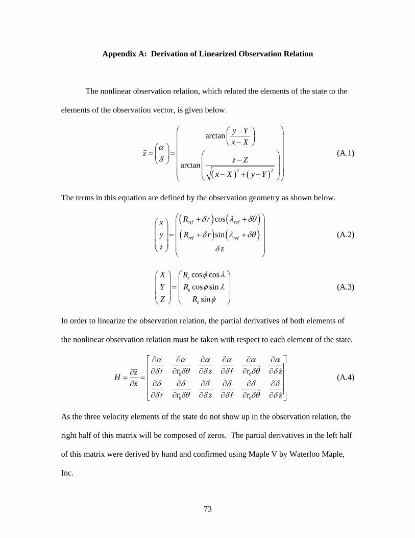
Appendix A: Derivation of Linearized Observation Relation
The nonlinear observation relation, which related the elements of the state to the
elements of the observation vector, is given below.
( ) ( )2 2
arctan
arctan
y Yx X
zz Z
x X y Y
αδ
⎛ −⎛ ⎞⎜ ⎟⎜ ⎟−⎝ ⎠⎜ ⎟⎛ ⎞
= = ⎜ ⎟⎜ ⎟ ⎛ −⎝ ⎠ ⎜ ⎟⎜ ⎟⎜ ⎟⎜ ⎟⎜ ⎟− + −⎝ ⎠⎝ ⎠
⎞
⎞ (A.1)
The terms in this equation are defined by the observation geometry as shown below.
( ) ( )( ) (
cos
sin
ref ref
ref ref
R rxy R rz z
)δ λ δθ
δ λ δθ
δ
⎛ ⎞+ +⎛ ⎞ ⎜ ⎟⎜ ⎟ ⎜= + +⎜ ⎟ ⎜ ⎟⎜ ⎟ ⎜ ⎟⎝ ⎠
⎝ ⎠
⎟ (A.2)
cos coscos sin
sin
e
e
e
X RY RZ R
φ λφ λφ
⎛ ⎞ ⎛ ⎞⎜ ⎟ ⎜ ⎟=⎜ ⎟ ⎜ ⎟⎜ ⎟ ⎜ ⎟⎝ ⎠ ⎝ ⎠
(A.3)
In order to linearize the observation relation, the partial derivatives of both elements of
the nonlinear observation relation must be taken with respect to each element of the state.
0 0
0 0
r r z r r zzHx
r r z r r z
α α α α α αδ δθ δ δ δθ δδ δ δ δ δ δδ δθ δ δ δθ δ
∂ ∂ ∂ ∂ ∂ ∂⎡ ⎤⎢ ⎥∂ ∂ ∂ ∂ ∂ ∂∂ ⎢ ⎥= =∂ ∂ ∂ ∂ ∂ ∂⎢ ⎥∂
⎢ ⎥∂ ∂ ∂ ∂ ∂ ∂⎣ ⎦
(A.4)
As the three velocity elements of the state do not show up in the observation relation, the
right half of this matrix will be composed of zeros. The partial derivatives in the left half
of this matrix were derived by hand and confirmed using Maple V by Waterloo Maple,
Inc.
73

( )( ) ( )
( ) ( ) ( )( ) ( )
( ) ( )( ) ( )
2
1 2
2
sin cos sin cossin
cos cos cos cos cos cos
sin cos sin1
cos cos cos
ref ref e refref
ref ref e ref ref e
ref ref e
ref ref e
R r R
R r R R r RH
r R r R
R r R
δ λ δθ φ λ λ δθλ δθ
δ λ δθ φ λ δ λ δθ φ λαδ δ λ δθ φ λ
δ λ δθ φ λ
⎡ ⎤+ + − ++ ⎣ ⎦−+ + − ⎡ ⎤+ + −∂ ⎣ ⎦= =
∂ ⎡ ⎤+ + −⎣ ⎦+⎡ ⎤+ + −⎣ ⎦
( ) ( )( ) ( )
( ) ( ) ( ) ( )( ) ( )
( ) ( )( ) ( )
2
2 20
sin cos sin sincos
cos cos cos cos cos cos
sin cos sin1
cos cos co
ref ref e ref refref ref
ref ref e ref ref e
ref ref e
ref ref e
R r R R rR r
R r R R r RH
r R r R
R r R
δ λ δθ φ λ δ λ δδ λ δθ
δ λ δθ φ λ δ λ δθ φ λαδθ δ λ δθ φ λ
δ λ δθ φ
⎡ ⎤+ + − + ++ + ⎣ ⎦−+ + − ⎡ ⎤+ + −∂ ⎣ ⎦= =
∂ ⎡ ⎤+ + −⎣ ⎦++ + −
θ
2sλ⎡ ⎤⎣ ⎦
3 0Hzαδ∂
= =∂
( ) ( ) ( ) ( )( )
( ) ( ) ( ) ( )
( ) ( ) ( )
2
2 2
4
sin cos cos cos cos...
sin1
cos cos cos sin cos sin
sin sin cos sin sin
e ref ref e ref
e
ref ref e ref ref e
e ref ref e r
z R R r R
z R
R r R R r R
z R R r R
Hr
δ φ δ λ δθ φ λ λ δθ
δ φ
δ λ δθ φ λ δ λ δθ φ λ
δ φ δ λ δθ φ λ λ
δδ
⎡ ⎤− − + + − +⎣ ⎦⎛ ⎞−⎜ ⎟+⎜ ⎟⎡ ⎤ ⎡⎜ ⎟+ + − + + + −⎣ ⎦ ⎣⎝ ⎠
⎡ ⎤− + + −⎣ ⎦−
∂= =∂
( )( )
( ) ( ) ( ) ( )
⎤⎦
( ) ( ) ( ) ( )( )
2
2 2
32 2 2
sin1
cos cos cos sin cos sin
cos cos cos sin cos sin
ef
e
ref ref e ref ref e
ref ref e ref ref e
z R
R r R R r R
R r R R r R
δθ
δ φ
δ λ δθ φ λ δ λ δθ φ λ
δ λ δθ φ λ δ λ δθ φ λ
⎛ ⎞⎜ ⎟⎜ ⎟⎜ ⎟⎜ ⎟⎜ ⎟⎜ ⎟⎜ ⎟⎜ ⎟+⎜ ⎟⎜ ⎟⎛ ⎞−⎜ ⎟⎜ ⎟+⎜ ⎟⎜ ⎟⎡ ⎤ ⎡⎜ ⎟+ + − + + + −⎜ ⎟⎣ ⎦ ⎣⎝ ⎠⎜ ⎟⎝ ⎠
⎡ ⎤ ⎡+ + − + + + −⎣ ⎦ ⎣
⎤⎦
⎤⎦
( ) ( ) ( ) ( ) ( )( )
( ) ( ) ( ) ( )
( ) ( ) ( )
2
2 2
50
sin cos cos cos sin
sin1
cos cos cos sin cos sin
sin sin cos sin
e ref ref e ref ref
e
ref ref e ref ref e
e ref ref e
z R R r R R r
z R
R r R R r R
z R R r R
Hr
δ φ δ λ δθ φ λ δ λ δθ
δ φ
δ λ δθ φ λ δ λ δθ φ λ
δ φ δ λ δθ φ λ
δδθ
⎡ ⎤− + + − + +⎣ ⎦⎛ ⎞−⎜ ⎟+⎜ ⎟⎡ ⎤ ⎡⎜ ⎟+ + − + + + −⎣ ⎦ ⎣⎝ ⎠
⎡ ⎤− + + −⎣ ⎦−
∂= =∂
( ) ( )( )
( ) ( ) ( ) ( )
⎤⎦
( ) ( ) ( ) ( )
2
2 2
2
cos
sin1
cos cos cos sin cos sin
cos cos cos sin cos sin
ref ref
e
ref ref e ref ref e
ref ref e ref ref e
R r
z R
R r R R r R
R r R R r R
δ λ δθ
δ φ
δ λ δθ φ λ δ λ δθ φ λ
δ λ δθ φ λ δ λ δθ φ λ
⎛ ⎞⎜ ⎟⎜ ⎟⎜ ⎟⎜ ⎟⎜ ⎟⎜ ⎟⎜ ⎟⎜ ⎟+ +⎜ ⎟⎜ ⎟⎛ ⎞−⎜ ⎟⎜ ⎟+⎜ ⎟⎜ ⎟⎡ ⎤ ⎡⎜ ⎟+ + − + + + −⎜ ⎟⎣ ⎦ ⎣⎝ ⎠⎜ ⎟⎝ ⎠
⎡ ⎤+ + − + + + −⎣ ⎦( )
⎤⎦
32 2⎡ ⎤⎣ ⎦
74

( ) ( ) ( ) ( )( )[ ]
( ) ( ) ( ) ( )
12 2 2
62
2 2
cos cos cos sin cos sin
sin1
cos cos cos sin cos sin
ref ref e ref ref e
e
ref ref e ref ref e
R r R R r RH
z z R
R r R R r R
δ λ δθ φ λ δ λ δθ φ λδδ δ φ
δ λ δθ φ λ δ λ δθ φ λ
−
⎡ ⎤ ⎡+ + − + + + −⎣ ⎦ ⎣∂= =∂ ⎛ ⎞−⎜ ⎟+⎜ ⎟⎡ ⎤ ⎡⎜ ⎟+ + − + + + −⎣ ⎦ ⎣⎝ ⎠
⎤⎦
⎤⎦
These equations make up the nonlinear observation relation as shown below.
1 2 3
4 5 6
0 0 00 0 0
H H HzHH H Hx⎡ ⎤∂
= = ⎢∂ ⎣ ⎦⎥ (A.11)
75

Appendix B: MATLAB Code - test_data_generator2.m
function [time,ra,dec] = test_data_generator2 % Create a set of non-maneuver test observation data arranged % in nightly observing sessions. % % OUTPUTS: % time - a time vector in units of days % ra - a vector of right ascension data in radians % dec - a vector of declination data in radians % % USER CONTROLS: % Initial State: comment out lines 44 and 45 for a randomly % generated initial state. Hardcode initial state % in lines 48 - 53 % Observation Uncertainty: set in line 109 % % Brian Hirsch % Spring 2006 clc;clear % This program will use the phi matrix from the CW equations % to generate test data points of the state. It then converts % the state data points into observation data points and adds some % random error onto each point. The data will be arranged in tight % clumps with large spaces of time in between to simulate real data % taken from telescopes. % The following units are used throughout the program: % Distance -- Earth radii (6378.135 km) % Time -- Days (86400 s) % Angles -- radians Re = 1; % Radius of earth longref = 3; % Reference satellite longitude Rref = 6.6 * Re; % Reference satellite orbit radius latsite = 0.3456; % Latitude of observer longsite = 2.7122; % Longitude of observer % Create the initial state by assuming the satellite can be off % from the reference satellite by anywhere from 0 to 10 m and % 0 to 10 cm/s, in the positive or negative direction. %x(1:3,1) = -1.6e-6 + 2 * 1.6e-6 * rand(3,1); %x(4:6,1) = -0.0014 + 2 * 0.0014 * rand(3,1); % Create a random initial state x(1,1)= 1.567856e-6; x(2,1)= 1.567856e-8; x(3,1)= 7.839282e-7; x(4,1)= 0.00677; x(5,1)= 0.000542; x(6,1)= 0.001355;
76

% The time vector will be made up of times spaced about 5 min % apart for 2 hours with 22 hours between them. K = 0; a = 1; while K < 10 t(1,a:a+24) = K:0.0035:K+0.084; K = K + 0.92; a = a + 25; end % mean motion of geo satellite is about 1 rev/day n = 2*pi; % in rad/day % For each time point: for i = 2:length(t) % Input the phi matrix psi = n*t(i); phi = [4-3*cos(psi) 0 0 1/n*sin(psi) 2/n*(1-cos(psi)) 0;... 6*(sin(psi) - psi) 1 0 2/n*(cos(psi)-1) 4/n*sin(psi)-3/n*psi 0;... 0 0 cos(psi) 0 0 1/n*sin(psi);... 3*n*sin(psi) 0 0 cos(psi) 2*sin(psi) 0;... 6*n*(cos(psi) -1) 0 0 -2*sin(psi) -3+4*cos(psi) 0;... 0 0 -n*sin(psi) 0 0 cos(psi)]; % Update state vector x(:,i) = phi * x(:,1); end % Now convert the state vector onto an observation vector % Determine x,y,z position of satellite in ECF frame. xpos = (Rref + x(1,:)) .* cos(longref + x(2,:)/Rref); ypos = (Rref + x(1,:)) .* sin(longref + x(2,:)/Rref); zpos = x(3,:); % Determine X,Y,Z postion of observer in ECF frame. X = Re.*cos(latsite).*cos(longsite); Y = Re.*cos(latsite).*sin(longsite); Z = Re.*sin(latsite); % Convert to RA and dec (observation matrix, z) ra = atan2((ypos-Y),(xpos-X)); dec = atan2((zpos-Z),sqrt((xpos-X).^2.+(ypos-Y).^2)); % To simulate the observation uncertainty inherent in the % telescopes, we'll add a random component to the RA and Dec % values, based on the given covariance of the equipment used. % NOTE: 1 arcsec = 4.85e-6 rad angle_error = 1e-5; % Choose RA and Dec uncertainty (in rad)for i = 1:length(ra)
77

ra_err = -angle_error + 2*angle_error * rand; ra(1,i) = ra(1,i) + ra_err; dec_err = -angle_error + 2*angle_error * rand; dec(1,i) = dec(1,i) + dec_err; end % Output the time vector time = t;
78

Appendix C: MATLAB Code - man_data_generator2.m
function [time,ra,dec,t0_man] = man_data_generator2 % Create test observation data containing a manuever. % % OUTPUTS: % time - a time vector in units of days % ra - a vector of right ascension data in radians % dec - a vector of declination data in radians % t0_man - the time at which the maneuver occurs % % USER CONTROLS: % Initial State: comment out lines 45 and 46 for a % randomly generated initial state. % Hardcode initial state in lines 49 - 54 % Maneuver Time: set in line 81 % Maneuver Magnitude: set in line 92 % Observation Uncertainty: set in line 160 % % Brian Hirsch % Spring 2006 clc;clear; % This program will use the phi matrix from the CW equations % to generate test data points of the state. The state elements % are then converted into observation data points and some random % error is added into each point. % The following units are used throughout the program: % Distance -- Earth radii (6378.135 km) % Time -- Days (86400 s) % Angles -- radians Re = 1; % Radius of earth longref = 3; % Reference satellite longitude Rref = 6.6 * Re; % Reference satellite orbit radius latsite = 0.3456; % Latitude of observer longsite = 2.7122; % Longitude of observer % Create the initial state by assuming the satellite can be % off from the reference satellite by anywhere from 0 to 10 m % and 0 to 10 cm/s, in the positive or negative direction. %x(1:3,1) = -1.6e-6 + 2 * 1.6e-6 * rand(3,1); %x(4:6,1) = -0.0014 + 2 * 0.0014 * rand(3,1); % Or just arbitrarily pick an initial offset x(1,1)= 1.567856e-6; x(2,1)= 1.567856e-8; x(3,1)= 7.839282e-7; x(4,1)= 0.00677; x(5,1)= 0.000542; x(6,1)= 0.001355;
79

% For now, the time vector runs in 5 min increments for 10 days t = 0:0.0035:10; % mean motion of geo satellite is about 1 rev/day n = 2*pi; % in rad/day % For each time point: for i = 2:length(t) % Input the phi matrix psi = n*t(i); phi = [4-3*cos(psi) 0 0 1/n*sin(psi) 2/n*(1-cos(psi)) 0;... 6*(sin(psi) - psi) 1 0 2/n*(cos(psi)-1) 4/n*sin(psi)-3/n*psi 0;... 0 0 cos(psi) 0 0 1/n*sin(psi);... 3*n*sin(psi) 0 0 cos(psi) 2*sin(psi) 0;... 6*n*(cos(psi) -1) 0 0 -2*sin(psi) -3+4*cos(psi) 0;... 0 0 -n*sin(psi) 0 0 cos(psi)]; % Update state vector x(:,i) = phi * x(:,1); end % Set maneuver time choose_man_time = 4.998; % This is the chosen maneuver time % Since there may not be a data point at our exact desired % maneuver time, we'll find the closest one to it. man_index = find(abs(t-choose_man_time)==min(abs(t-choose_man_time))); t0_man = t(man_index); x0_man = x(:,man_index); % Now insert the maneuver into the state (in Earth radii per day. % 1 cm/s = 0.00013 earth radii/day. man_mag = -0.001; x0_man(5,1) = x0_man(5,1) + man_mag; % Now create a post-maneuver time vector that starts at the % manuever time and continues with the rest of the data. It als o% needs to be set such that the maneuver time is now time zero. t_man = t(man_index:length(t)); t_man = t_man - t0_man; % Now propogate the post-maneuver state with the phi matrix for i = 2:length(t_man) % Input the phi matrix psi = n*t(i); phi = [4-3*cos(psi) 0 0 1/n*sin(psi) 2/n*(1-cos(psi)) 0;... 6*(sin(psi) - psi) 1 0 2/n*(cos(psi)-1) 4/n*sin(psi)-3/n*psi 0;...
80

0 0 cos(psi) 0 0 1/n*sin(psi);... 3*n*sin(psi) 0 0 cos(psi) 2*sin(psi) 0;... 6*n*(cos(psi) -1) 0 0 -2*sin(psi) -3+4*cos(psi) 0;... 0 0 -n*sin(psi) 0 0 cos(psi)]; % Update state vector x(:,i+man_index-1) = phi * x0_man; end % The state has now been propagated in 5 min intervals for % about 10 days. Assume that real observations will occur in % segments of about 2 hours with around 22 hours between each % segment. We must therefore crop the state and time vector to % simulate this. % Pull out "daily" observation sessions and stick them together % into new time and state vectors K = 1; a = 1; while K < length(t) new_t(1,a:a+24) = t(1,K:K+24); new_x(:,a:a+24) = x(:,K:K+24); K = K + 239; a = a + 25; end % Now convert the state vector onto an observation vector % Determine x,y,z position of satellite in ECI frame. xpos = (Rref + new_x(1,:)) .* cos(longref + new_x(2,:)/Rref); ypos = (Rref + new_x(1,:)) .* sin(longref + new_x(2,:)/Rref); zpos = new_x(3,:); % Determine X,Y,Z postion of observer in ECI frame. X = Re.*cos(latsite).*cos(longsite); Y = Re.*cos(latsite).*sin(longsite); Z = Re.*sin(latsite); % Convert to RA and dec (observation matrix, z) ra = atan2((ypos-Y),(xpos-X)); dec = atan2((zpos-Z),sqrt((xpos-X).^2.+(ypos-Y).^2)); % To simulate the observation uncertainty inherent in the % telescopes, we'll add a random component to the RA and Dec % values, based on the given covariance of the equipment used. % NOTE: 1 arcsec = 4.85e-6 rad angle_error = 1e-5; % Choose RA and Dec uncertainty (in rad)for i = 1:length(ra) ra_err = -angle_error + 2*angle_error * rand; ra(1,i) = ra(1,i) + ra_err; dec_err = -angle_error + 2*angle_error * rand; dec(1,i) = dec(1,i) + dec_err; end time=new_t;
81

Appendix D: MATLAB Code - NLS_nonman_algorithm.m clear;clc;close all; % This is the main program of the thesis for non-maneuver % data. It reads in the observation data and fit a nonlinear % least squares curve to the observations data. % % USER CONTROLS: % Source Data - if the observation data is in an obscard % file, uncomment line 36 and comment out % line 39. If the data comes from the test % data generator, comment out line 36 and % use line 39. % % FUNCTIONS CALLED: % radec_read.m % test_data_generator2.m (Shown in Appendix B) % NLS_loop.m (Shown in Appendix F) % % Brian Hirsc h% Spring 2006 % The following units are used throughout the program: % Distance -- Earth radii (6378.135 km) % Time -- Days (86400 s) % Angles -- radians Re = 1; % Radius of earth longref = 3; % Reference satellite longitude Rref = 6.6 * Re; % Reference satellite orbit radius latsite = 0.3456; % Latitude of observer longsite = 2.7122; % Longitude of observer n = 2*pi; % mean motion of geo satellite is about 1 rev/day % Read in the test data from an obscard file %[time, ra, dec] = radec_read('testfile.obs'); % Read in data from the test data generator [t, ra, dec] = test_data_generator2; % Set initial guess of the state x0 = zeros(6,1); % Run Nonlinear Least Squares Loop [fixed_x0,G,H,r_total,sigma]=NLS_loop(t,ra,dec,x0); % Now convert the improved state vector into RA and Dec arrays so % it can be compared to the observation data % First propagate the improved initial state vector through all % the observation times
82

fixed_x(:,1) = fixed_x0; % Make a new time vector for the improved data that has more % data points in order to make a smoother curve. ti = 0:0.01:t(length(t)); % For each time point: for i = 2:length(ti) % Input the phi matrix psi = n*ti(i); phi = [4-3*cos(psi) 0 0 1/n*sin(psi) 2/n*(1-cos(psi)) 0;... 6*(sin(psi) - psi) 1 0 2/n*(cos(psi)-1) 4/n*sin(psi)-3/n*psi 0;... 0 0 cos(psi) 0 0 1/n*sin(psi);... 3*n*sin(psi) 0 0 cos(psi) 2*sin(psi) 0;... 6*n*(cos(psi) -1) 0 0 -2*sin(psi) -3+4*cos(psi) 0;... 0 0 -n*sin(psi) 0 0 cos(psi)]; % Update improved state vector fixed_x(:,i) = phi * fixed_x(:,1); end % Determine x,y,z position of satellite in ECF frame. xpos = (Rref + fixed_x(1,:)) .* cos(longref + fixed_x(2,:)/Rref); ypos = (Rref + fixed_x(1,:)) .* sin(longref + fixed_x(2,:)/Rref); zpos = fixed_x(3,:); % Determine the position of the observing site in ECF frame X = Re*cos(latsite)*cos(longsite); Y = Re*cos(latsite)*sin(longsite); Z = Re*sin(latsite); % Convert to RA and Dec fixed_ra = atan2((ypos-Y),(xpos-X)); fixed_dec = atan2((zpos-Z),sqrt((xpos-X).^2.+(ypos-Y).^2)); % Convert all RAs and Decs to milliradians ra_milli = 1000 .* ra; dec_milli = 1000 .* dec; fixed_ra_milli = 1000 .* fixed_ra; fixed_dec_milli = 1000 .* fixed_dec; %%%%%%%%%%%%%%%%%%%%%%%%%%%%%%%%%%%%%%%%%%%%%%%%%%%%%%%%% % Plot results %%%%%%%%%%%%%%%%%%%%%%%%%%%%%%%%%%%%%%%%%%%%%%%%%%%%%%%%% % First plot RA vs Dec, both observed data and NLS fitted data figure(1) subplot(2,2,1) plot(ra_milli,dec_milli,'x',fixed_ra_milli,fixed_dec_milli,'-r') xlabel('Right Ascension (milliradians)')
83

ylabel('Declination (milliradians)') legend('Observed RA and Dec 'NLS fitted RA and Dec',1) ',title('Satellite Position') grid on % Plot RA vs time, both observed data and NLS fitted data %figure(2) subplot(2,2,3) plot(t,ra_milli,'x',ti,fixed_ra_milli,'-r') xlabel('Time (days)') ylabel('Right Ascension (milliradians)') legend('Observed RA','NLS fitted RA',1) title('Right Ascension v. Time') grid on % Plot Dec vs time, both observed data and NLS fitted data %figure(3) subplot(2,2,4) plot(t,dec_milli,'x',ti,fixed_dec_milli,'-r') xlabel('Time (days)') ylabel('Declination (milliradians)') legend('Observed Dec','NLS fitted Dec',1) title('Declination v. Time') grid on
84

Appendix E: MATLAB Code - NLS_man_algorithm.m
clear;clc;close all; % This is the main program of the thesis for maneuver data. % It reads in the observation data and separates it into a pre-maneuver % partition and a post-maneuver partition. The program then fits a % nonlinear least squares curve to each set of data, determines the % intersection points between these two fits, and estimates the % maneuver time and vector based on these intersections. % % USER CONTROLS: % Source Data - if the observation data is in an obscard file, % uncomment line 38 and comment out line 41. % If the data comes from the test data generator, % comment out line 38 and use line 41. % % FUNCTIONS CALLED: % radec_read.m % man_data_generator2.m (Shown in Appendix C) % pre_post_man_separate.m (Shown in Appendix H) % NLS_loop.m (Shown in Appendix F) % possible_man_times.m (Shown in Appendix K) % % Brian Hirsch % Spring 2006 % The following units are used throughout the program: % Distance -- Earth radii (6378.135 km) % Time -- Days (86400 s) % Angles -- radians Re = 1; % Radius of earth longref = 3; % Reference satellite longitude Rref = 6.6 * Re; % Reference satellite orbit radius latsite = 0.3456; % Latitude of observer longsite = 2.7122; % Longitude of observer n = 2*pi; % mean motion of geo satellite is about 1 rev/day % Read in the test data from an obscard file %[time, ra, dec] = radec_read('testfile.obs'); % Read in data from the test data generator [t,ra,dec] = man_data_generator2; numdata = length(t); % The man_time_check program will go through this data, determine % between which data points the maneuver took place, and separate % the data into pre-maneuver data and post-maneuver data. [pre_man_t,pre_man_ra,pre_man_dec,post_man_t,post_man_ra,post_man_dec,man_type]=pre_post_man_separate(t,ra,dec); % Now an NLS loop will be run for both the pre and post maneuever % data.
85

% Set initial guess of the state (for both sets of data) x0 = zeros(6,1); % Run Nonlinear Least Squares Loop (for both data sets) [fixed_x0_pre,G_pre,H_pre,r_total_pre,sigma_pre]=NLS_loop(pre_man_t,pre_man_ra,pre_man_dec,x0); [fixed_x0_post,G_pre,H_post,r_total_post,sigma_post]=NLS_loop(post_man_t,post_man_ra,post_man_dec,x0); % Now convert the improved state vector into RA and Dec arrays so % it can be compared to the observation data. % First propagate the improved initial state vector through all the % observation times fixed_x_pre(:,1) = fixed_x0_pre; fixed_x_post(:,1) = fixed_x0_post; % Make a new time vector for the improved data that has more data % points in order to make a smoother curve. ti = 0:0.01:t(length(t)); % For each time point: for i = 2:length(ti) % Input the phi matrix psi = n*ti(i); phi = [4-3*cos(psi) 0 0 1/n*sin(psi) 2/n*(1-cos(psi)) 0;... 6*(sin(psi) - psi) 1 0 2/n*(cos(psi)-1) 4/n*sin(psi)-3/n*psi 0;... 0 0 cos(psi) 0 0 1/n*sin(psi);... 3*n*sin(psi) 0 0 cos(psi) 2*sin(psi) 0;... 6*n*(cos(psi) -1) 0 0 -2*sin(psi) -3+4*cos(psi) 0;... 0 0 -n*sin(psi) 0 0 cos(psi)]; % Update improved state vector fixed_x_pre(:,i) = phi * fixed_x_pre(:,1); fixed_x_post(:,i) = phi * fixed_x_post(:,1); end % Determine x,y,z position of satellite in ECF frame. xpos_pre = (Rref + fixed_x_pre(1,:)) .* cos(longref + fixed_x_pre(2,:)/Rref); ypos_pre = (Rref + fixed_x_pre(1,:)) .* sin(longref + fixed_x_pre(2,:)/Rref); zpos_pre = fixed_x_pre(3,:); xpos_post = (Rref + fixed_x_post(1,:)) .* cos(longref + fixed_x_post(2,:)/Rref); ypos_post = (Rref + fixed_x_post(1,:)) .* sin(longref + fixed_x_post(2,:)/Rref); zpos_post = fixed_x_post(3,:); % Determine the position of the observing site in ECF frame X = Re*cos(latsite)*cos(longsite); Y = Re*cos(latsite)*sin(longsite); Z = Re*sin(latsite);
86

% Convert to RA and Dec fixed_ra_pre = atan2((ypos_pre-Y),(xpos_pre-X)); fixed_dec_pre = atan2((zpos_pre-Z),sqrt((xpos_pre-X).^2.+(ypos_pre-Y).^2)); fixed_ra_post = atan2((ypos_post-Y),(xpos_post-X)); fixed_dec_post = atan2((zpos_post-Z),sqrt((xpos_post-X).^2.+(ypos_post-Y).^2)); % Convert all RAs and Decs to milliradians ra_milli = 1000 .* ra; dec_milli = 1000 .* dec; fixed_ra_milli_pre = 1000 .* fixed_ra_pre; fixed_dec_milli_pre = 1000 .* fixed_dec_pre; fixed_ra_milli_post = 1000 .* fixed_ra_post; fixed_dec_milli_post = 1000 .* fixed_dec_post; %%%%%%%%%%%%%%%%%%%%%%%%%%%%%%%%%%%%%%%%%%%%%%%%%%%%%%%%%%%%%%%% % Plot results %%%%%%%%%%%%%%%%%%%%%%%%%%%%%%%%%%%%%%%%%%%%%%%%%%%%%%%%%%%%%%%% % First plot RA vs Dec, both observed data and NLS fitted data figure subplot(2,2,1) plot(ra_milli,dec_milli,'xk',fixed_ra_milli_pre,fixed_dec_milli_pre,'-r',fixed_ra_milli_post,fixed_dec_milli_post,'-b') xlabel('Right Ascension (milliradians)') ylabel('Declination (milliradians)') legend('Observed RA and Dec','Pre-maneuver NLS fit','Post-maneuver NLS fit',1) title('a) Satellite Position') grid on % Plot RA vs time, both observed data and NLS fitted data subplot(2,2,3) plot(t,ra_milli,'xk',ti,fixed_ra_milli_pre,'-r',ti,fixed_ra_milli_post,'-b') xlabel('Time (days)') ylabel('Right Ascension (milliradians)') legend('Observed RA','Pre-maneuver NLS fit','Post-maneuver NLS fit',1) title('b) Right Ascension v. Time') grid on % Plot Dec vs time, both observed data and NLS fitted data subplot(2,2,4) plot(t,dec_milli,'xk',ti,fixed_dec_milli_pre,'-r',ti,fixed_dec_milli_post,'-b') xlabel('Time (days)') ylabel('Declination (milliradians)') legend('Observed Dec','Pre-maneuver NLS fit','Post-maneuver NLS fit',1) title('c) Declination v. Time') grid on
87

% The maneuver time can be determined by finding where the % pre-maneuver and post-maneuver NLS curves intersect. However, % the curves may intersect at multiple points since they are % sinusoidal. We must therefore pull out each intersection, look at % the velocity change for each, and determine which velocity change % looks the most like a reasonable maneuver, where a reasonable % maneuver is one that is almost totally in the North-South % direction, or almost totally in the East-West direction. [pos_min_times,pos_min_indeces]=possible_man_times(fixed_ra_pre,fixed_ra_post,fixed_dec_pre,fixed_dec_post,ti,man_type); % We can set a constraint that the maneuver must occur near the % pre-post maneuver separation point, since all the possible N-S % maneuver are identical. We'll set the range to a day before and % after the separation point min_man_time = post_man_t(1,1) - 1; max_man_time = post_man_t(1,1) + 1; % Only keep the possible min times that fall within this range. c = 1; % counter for i = 1:length(pos_min_times) if pos_min_times(1,i) > min_man_time && pos_min_times(1,i) < max_man_time min_times(1,c) = pos_min_times(1,i); c = c + 1; end end % If no maneuver took place during the time span of the % observations, the program will generally start to break down % here, because this constraint will knock out all possible min % times. Rather than allowing the program to crash, we'll just % keep all the possible min times and note that the error occurred, % meaning there may be no maneuver at all. Since the above % constraint isn't necessary for E-W maneuvers, we'll also keep all % intersections if the maneuver was an E-W one. if c ==1 || man_type == 1 min_times = pos_min_times; end % For each intersection time, determine the state from the % pre-maneuver fit and from the post-maneuver fit, by propagating % to each intersection time with the phi matrix % For each intersection: for i = 1:length(min_times) % Input the phi matrix psi = n*min_times(1,i); phi = [4-3*cos(psi) 0 0 1/n*sin(psi) 2/n*(1-cos(psi)) 0;... 6*(sin(psi) - psi) 1 0 2/n*(cos(psi)-1) 4/n*sin(psi)-3/n*psi 0;... 0 0 cos(psi) 0 0 1/n*sin(psi);...
88

3*n*sin(psi) 0 0 cos(psi) 2*sin(psi) 0;... 6*n*(cos(psi) -1) 0 0 -2*sin(psi) -3+4*cos(psi) 0;... 0 0 -n*sin(psi) 0 0 cos(psi)]; pre_man_state(:,i) = phi*fixed_x0_pre; post_man_state(:,i) = phi*fixed_x0_post; end % We're only concerned with the velocity difference, so pull % those out pre_man_vel = pre_man_state(4:6,:); post_man_vel = post_man_state(4:6,:); % Determine the difference between the pre and post maneuver % velocities man_vel_diff = abs(post_man_vel-pre_man_vel); % Determine the magnitude of the total velocity difference for i = 1:length(min_times) tot_vel_diff(1,i) = sqrt((man_vel_diff(1,i))^2+(man_vel_diff(2,i))^2+(man_vel_diff(3,i))^2); end avg_vel_diff = mean(tot_vel_diff); % Now we want to determine which of the velocity differences % for each intersection most closely resembles an all E-W % difference, or an all N-S difference. This will be done by % dividing the velocity change in the direction of interest % (N-S or E-W) by the magnitude of the total velocity change. for i = 1:length(min_times) % 1st row checks E-W changes E_W_man_match(1,i) = man_vel_diff(2,i)/tot_vel_diff(1,i); % 2nd row checks N-S changes N_S_man_match(1,i) = man_vel_diff(3,i)/tot_vel_diff(1,i); end % Find the max value [max_value,max_index]=max(max(E_W_man_match,N_S_man_match)); % Output the maneuver and time of maneuver (only if the program % thinks a maneuver actually occured) if c ~= 1 && avg_vel_diff > 1e-5 % If a maneuver was detected, % output it Time_of_Maneuver = min_times(1,max_index) Maneuver = post_man_vel(:,max_index) - pre_man_vel(:,max_index) else % If no maneuver was detected, say so, but continue % running the program display('No valid maneuver time was detected. Try running this data through the non-maneuver NLS model.') Time_of_Maneuver = min_times(1,max_index); Maneuver = post_man_vel(:,max_index) - pre_man_vel(:,max_index); end
89

% Make a final plot showing the actual path of the satellite, % according to the NLS fit. time_sep_index = pos_min_indeces(1,find(pos_min_times == Time_of_Maneuver)); t_pre = ti(1,1:time_sep_index); t_post = ti(1,time_sep_index:length(ti)); % Now we'll truncate the pre-maneuver and post-maneuver at the % maneuver time. final_fit_ra_milli(1,1:time_sep_index) = fixed_ra_milli_pre(1,1:time_sep_index); final_fit_dec_milli(1,1:time_sep_index) = fixed_dec_milli_pre(1,1:time_sep_index); final_fit_ra_milli(1,time_sep_index:length(ti)) = fixed_ra_milli_post(1,time_sep_index:length(ti)); final_fit_dec_milli(1,time_sep_index:length(ti)) = fixed_dec_milli_post(1,time_sep_index:length(ti)); % Now plot this: % First plot RA vs Dec, both observed data and NLS fitted data figure subplot(2,2,1) plot(ra_milli,dec_milli,'xk',final_fit_ra_milli,final_fit_dec_milli,'-r') xlabel('Right Ascension (milliradians)') ylabel('Declination (milliradians)') legend('Observed Position','NLS fitted Position',1) title('a) Satellite Position') grid on % Plot RA vs time, both observed data and NLS fitted data subplot(2,2,3) plot(t,ra_milli,'xk',ti,final_fit_ra_milli,'-r') xlabel('Time (days)') ylabel('Right Ascension (milliradians)') legend('Observed RA','NLS fitted RA',1) title('b) Right Ascension v. Time') grid on % Plot Dec vs time, both observed data and NLS fitted data subplot(2,2,4) plot(t,dec_milli,'xk',ti,final_fit_dec_milli,'-r') xlabel('Time (days)') ylabel('Declination (milliradians)') legend('Observed Dec','NLS fitted Dec',1) title('c) Declination v. Time') grid on
90

Appendix F: MATLAB Code - NLS_loop.m
function [fixed_x0,G,H,r_total,sigma]=NLS_loop(t,ra,dec,x0) % NLS_loop % This function runs through the nonlinear least squares loop % % INPUTS: % t - time vector (1 x n) % ra - right ascension vector (1 x n) % dec - declination vector (1 x n) % x0 - guess of initial state (6 x 1) % % OUTPUTS: % fixed_x0 - converged estimate of initial state % G - observation relation matrix % H - linearized observation relation matrix % r_total - gives the ra and dec residuals for each data % point. Each pair of rows corresponds to a data % point and each column corresponds to an interation % of the NLS loop (2n x # of iterations) % sigma - gives the covariance of each element of the % fitted state % % FUNCTIONS CALLED: % obs_matrix.m (Shown in Appendix G) % % Brian Hirsch % Spring 2006 numdata = length(t); %%%%%%%%%%%%%%%%%%%%%%%%%%%%%%%%%%%%%%%%%%%%%%%%%%%%%%%%%%%%% % Nonlinear Least Squares Loop % %%%%%%%%%%%%%%%%%%%%%%%%%%%%%%%%%%%%%%%%%%%%%%%%%%%%%%%%%%%%% % Set a maximum number of iterations maxiter = 40; for iter = 1:maxiter % Initialize vectors and matrices zob = zeros(2,1); % The vector of RA and Dec Q = eye(2,2); % The covariance matrix Q(1,1) = 4.848e-6^2; % Assume covariance of both RA and Dec is Q(2,2) = 4.848e-6^2; % 1 arcsec^2 or 4.848e-6^2 rad^2 Pinv = zeros(6,6); % Running sums used in the observation CorVect = zeros(6,1); % iteration % Run a loop to process each observation for obiter = 1:numdata
91

% Pull out individual observations tob = t(obiter); zob = [ra(obiter);dec(obiter)]; % Propagate the state forward to the correct time % Define the state transition matrix using the standard CW eqns. n = 2*pi; % mean motion of geo satellite is about 1 rev/day psi = n*tob; phi = [4-3*cos(psi) 0 0 1/n*sin(psi) 2/n*(1-cos(psi)) 0;... 6*(sin(psi) - psi) 1 0 2/n*(cos(psi)-1) 4/n*sin(psi)-3/n*psi 0;... 0 0 cos(psi) 0 0 1/n*sin(psi);... 3*n*sin(psi) 0 0 cos(psi) 2*sin(psi) 0;... 6*n*(cos(psi) -1) 0 0 -2*sin(psi) -3+4*cos(psi) 0;... 0 0 -n*sin(psi) 0 0 cos(psi)]; x = phi*x0; % Now get the G and H matrices [G,H] = obs_matrix(x); % Calculate residual vector (r_total contains residuals for all % iterations) r = zob - G; r_total(obiter*2-1:obiter*2,iter) = r; % Calculate the observation matrix, T. T = H * phi; % Form running sums of: % Pinv = transpose(T)*inverse(Q)*T % CorVect = transpose(t)*inverse(Q)*r Pinv = Pinv + T'*inv(Q)*T; CorVect = CorVect + T'*inv(Q)*r; end % Finished looping through observations %%%%%%%%%%%%%%%%%%%%%%%%%%%%%%%%%%%%%%% % Now improve the state estimate % Determine covariance matrix, P P = inv(Pinv); % Determine correction to the state dx = P * CorVect; % Update initial state x0 = x0 + dx; end
92

% End of least squares loop fixed_x0 = x0; % Check covariance of estimated state sigma(:,1) = [sqrt(P(1,1));sqrt(P(2,2));sqrt(P(3,3));sqrt(P(4,4));sqrt(P(5,5));sqrt(P(6,6))];
93

Appendix G: MATLAB Code - obs_matrix.m function [G,H] = obs_matrix(x) % This function calculates the observation relation, G, and % the linearized observation relation, H. % % OUTPUTS: % G - observation relation % H - linearized observation relation % % INPUTS: % x - 6x1 state vector % % Brian Hirsc h% Spring 2006 % The equations for H were derived using the math software, % Maple V, and confirmed by a hand derivation. % The following units are used throughout the program: % Distance -- Earth radii (6378.135 km) % Time -- Days (86400 s) % Angles -- radians % The given values needed for this approximation include: Re = 1; % Radius of earth longref = 3; % Reference satellite longitude Rref = 6.6 * Re; % Reference satellite orbit radius latsite = 0.3456; % Latitude of observer longsite = 2.7122; % Longitude of observer n = 2*pi; % mean motion of geo satellite is about 1 rev/day % Pull out the state vector delr = x(1); deltheta = x(2) / Rref; delz = x(3); delrdot = x(4); delthetadot = x(5) / Rref; delzdot = x(6); % Determine the position of the observing site in ECI frame X = Re*cos(latsite)*cos(longsite); Y = Re*cos(latsite)*sin(longsite); Z = Re*sin(latsite); % Determine the position of the reference satellite in ECI frame xpos = (Rref + delr)*cos(longref + deltheta); ypos = (Rref + delr)*sin(longref + deltheta); zpos = delz; % RA and Dec will be the observation variables. They are defined % below in terms of the positions of the observer (X,Y,Z) and the % reference satellite (xpos,ypos,zpos).
94

G = [atan2((ypos-Y),(xpos-X)) ; atan2((zpos-Z),sqrt((xpos-X)^2+(ypos-Y)^2))]; % The H matrix is the derivate of the observation vector, z, % with respect to the state vector. Note that half the matrix % will be zeros since the derivatives with respect to the velocities % in the state vector are zero. % H1 = diff(RA,delr) H1 = (sin(longref+deltheta)/((Rref+delr)*cos(longref+deltheta)-Re*cos(latsite)*cos(longsite))-((Rref+delr)*sin(longref+deltheta)-Re*cos(latsite)*sin(longsite))*cos(longref+deltheta)/(((Rref+delr)*cos(longref+deltheta)-Re*cos(latsite)*cos(longsite))^2))/(1+((Rref+delr)*sin(longref+deltheta)-Re*cos(latsite)*sin(longsite))^2/(((Rref+delr)*cos(longref+deltheta)-Re*cos(latsite)*cos(longsite))^2)); % H2 = diff(RA,deltheta) H2 = ((Rref+delr)*cos(longref+deltheta)/((Rref+delr)*cos(longref+deltheta)-Re*cos(latsite)*cos(longsite))+((Rref+delr)*sin(longref+deltheta)-Re*cos(latsite)*sin(longsite))*(Rref+delr)*sin(longref+deltheta)/(((Rref+delr)*cos(longref+deltheta)-Re*cos(latsite)*cos(longsite))^2))/(1+((Rref+delr)*sin(longref+deltheta)-Re*cos(latsite)*sin(longsite))^2/(((Rref+delr)*cos(longref+deltheta)-Re*cos(latsite)*cos(longsite))^2)); % H3 = diff(RA,delz) H3 = 0; % H4 = diff(Dec,delr) H4 = -1/2*(delz-Re*sin(latsite))*(2*((Rref+delr)*cos(longref+deltheta)-Re*cos(latsite)*cos(longsite))*cos(longref+deltheta)+2*((Rref+delr)*sin(longref+deltheta)-Re*cos(latsite)*sin(longsite))*sin(longref+deltheta))/((((Rref+delr)*cos(longref+deltheta)-Re*cos(latsite)*cos(longsite))^2+((Rref+delr)*sin(longref+deltheta)-Re*cos(latsite)*sin(longsite))^2)^(3/2)*(1+(delz-Re*sin(latsite))^2/(((Rref+delr)*cos(longref+deltheta)-Re*cos(latsite)*cos(longsite))^2+((Rref+delr)*sin(longref+deltheta)-Re*cos(latsite)*sin(longsite))^2))); % H5 = diff(Dec,deltheta) H5 = -1/2*(delz-Re*sin(latsite))*(-2*((Rref+delr)*cos(longref+deltheta)-Re*cos(latsite)*cos(longsite))*(Rref+delr)*sin(longref+deltheta)+2*((Rref+delr)*sin(longref+deltheta)-Re*cos(latsite)*sin(longsite))*(Rref+delr)*cos(longref+deltheta))/((((Rref+delr)*cos(longref+deltheta)-Re*cos(latsite)*cos(longsite))^2+((Rref+delr)*sin(longref+deltheta)-Re*cos(latsite)*sin(longsite))^2)^(3/2)*(1+(delz-Re*sin(latsite))^2/(((Rref+delr)*cos(longref+deltheta)-Re*cos(latsite)*cos(longsite))^2+((Rref+delr)*sin(longref+deltheta)-Re*cos(latsite)*sin(longsite))^2)));
95

% H6 = diff(Dec,delz) H6 = 1/(sqrt(((Rref+delr)*cos(longref+deltheta)-Re*cos(latsite)*cos(longsite))^2+((Rref+delr)*sin(longref+deltheta)-Re*cos(latsite)*sin(longsite))^2)*(1+(delz-Re*sin(latsite))^2/(((Rref+delr)*cos(longref+deltheta)-Re*cos(latsite)*cos(longsite))^2+((Rref+delr)*sin(longref+deltheta)-Re*cos(latsite)*sin(longsite))^2))); % Build H matrix H = [H1 H2 H3 0 0 0; H4 H5 H6 0 0 0];
96

Appendix H: MATLAB Code - pre_post_man_separate.m function [pre_man_t,pre_man_ra,pre_man_dec,post_man_t,post_man_ra,post_man_dec,man_type]=pre_post_man_separate(t,ra,dec) % This function will determine between which clumps of observations % the manuever takes place. We'll get an initial NLS fit from just % the first clump of data, or the first two clumps of data. This % should produce a trajectory that somewhat lines up with the % pre-maneuever data. We should then be able to determine the % maneuever by checking for a jump in the residuals when we include % the entire data set. % % INPUTS: % t - entire time vector (in days) of observations % ra - entire right ascension vector % dec - entire declination vector % % OUTPUTS: % pre_man_t - Pre-maneuver half of the time vector % pre_man_ra - Pre-maneuver half of the ra vector % pre_man_dec - Pre-maneuver half of the dec vector % post_man_t - Post-maneuver half of the time vector % post_man_ra - Post-maneuver half of the ra vector % post_man_dec - Post-maneuver half of the dec vector % man_type - Maneuver type: 1 for East-West maneuver, % 2 for North-South maneuver % USER CONTROLS: % Line 95 or 98 must be commented out depending on whether % the 1st clump or both the 1st and 2nd clumps will be used % to create an initial NLS fit % % FUNCTIONS CALLED % NLS_loop.m (Shown in Appendix F) % ra_man_check (Shown in Appendix J) % dec_man_check (Shown in Appendix I) % % Brian Hirsch % Spring 2006 % Pull out first clump of data. % First determine the step size of the first clump of observations clump_step = t(1,2) - t(1,1); % Form a new time vector that only contains the first clump of data t_1st(1,1) = t(1,1); % Now determine how long the clump goes. i=2; while t(1,i) - t(1,i-1) <= 2 * clump_step %Doubled to give wiggle room t_1st(1,i) = t(1,i); i = i + 1; end
97

% Now crop the ra and dec vectors so only the 1st clump of data is % used for c = 1:length(t_1st) ra_1st(1,c) = ra(1,c); dec_1st(1,c) = dec(1,c); end % Now pull out the second clump of data % First form a vector containing only the 2nd clump of time data t_2nd(1,1) = t(1,length(t_1st)+1); i=2; b = length(t_1st) + 2; while t(1,b) - t(1,b-1) <= 2 * clump_step %Doubled to give wiggle room t_2nd(1,i) = t(1,b); i = i + 1; b = b + 1; end % Crop the ra and dec vectors so only the 2nd clump of data is used i=1; for c = (length(t_1st)+1):(length(t_1st)+length(t_2nd)) ra_2nd(1,i) = ra(1,c); dec_2nd(1,i) = dec(1,c); i = i + 1; end % Now combine 1st and 2nd clumps of data into one t_1st_and_2nd = [t_1st t_2nd]; ra_1st_and_2nd = [ra_1st ra_2nd]; dec_1st_and_2nd = [dec_1st dec_2nd]; % Now we'll run a NLS fit to the first (or 1st and 2nd) clump % of data. % Create an initial guess x0 = zeros(6,1); % Run NLS loop for either the 1st clump of data or the 1st and % 2nd clumps (comment one or the other out) % Using just the first clump %[fixed_x0,G,H,r_total,sigma]=NLS_loop(t_1st,ra_1st,dec_1st,x0); % Using the first and second clump [fixed_x0,G,H,r_total,sigma]=NLS_loop(t_1st_and_2nd,ra_1st_and_2nd,dec_1st_and_2nd,x0); %%%%%%%%%%%%%%%%%%%%%%%%%%%%%%%%%%%%%%%%%%%%%%%%%%%%%%%%%%%%%%%%%% % Plot the fit to the first data clump against all the data to see % if a maneuver is visible.
98

% First propagate the fitted initial state over the length of the % time vector % Make a new time vector for the improved data that has more data % points in order to make a smoother curve. ti = 0:0.01:t(length(t)); fixed_x(:,1) = fixed_x0; % For each time point: for i = 2:length(ti) % Input the phi matrix n = 2*pi; % mean motion of geo satellite is about 1 rev/day psi = n*ti(i); phi = [4-3*cos(psi) 0 0 1/n*sin(psi) 2/n*(1-cos(psi)) 0;... 6*(sin(psi) - psi) 1 0 2/n*(cos(psi)-1) 4/n*sin(psi)-3/n*psi 0;... 0 0 cos(psi) 0 0 1/n*sin(psi);... 3*n*sin(psi) 0 0 cos(psi) 2*sin(psi) 0;... 6*n*(cos(psi) -1) 0 0 -2*sin(psi) -3+4*cos(psi) 0;... 0 0 -n*sin(psi) 0 0 cos(psi)]; % Update improved state vector fixed_x(:,i) = phi * fixed_x(:,1); end % Given physical values Re = 1; % Radius of earth longref = 3; % Reference satellite longitude Rref = 6.6 * Re; % Reference satellite orbit radius latsite = 0.3456; % Latitude of observer longsite = 2.7122; % Longitude of observer % Determine x,y,z position of satellite in ECF frame. xpos = (Rref + fixed_x(1,:)) .* cos(longref + fixed_x(2,:)/Rref); ypos = (Rref + fixed_x(1,:)) .* sin(longref + fixed_x(2,:)/Rref); zpos = fixed_x(3,:); % Determine the position of the observing site in ECF frame X = Re*cos(latsite)*cos(longsite); Y = Re*cos(latsite)*sin(longsite); Z = Re*sin(latsite); % Convert to RA and Dec fixed_ra = atan2((ypos-Y),(xpos-X)); fixed_dec = atan2((zpos-Z),sqrt((xpos-X).^2.+(ypos-Y).^2)); % Convert all RAs and Decs to milliradians ra_milli = 1000 .* ra; dec_milli = 1000 .* dec; fixed_ra_milli = 1000 .* fixed_ra; fixed_dec_milli = 1000 .* fixed_dec;
99

%%%%%%%%%%%%%%%% % Plot results %%%%%%%%%%%%%%%% % First plot RA vs Dec, both observed data and NLS fitted data figure subplot(2,2,1) plot(ra_milli,dec_milli,'x',fixed_ra_milli,fixed_dec_milli,'-r') xlabel('Right Ascension (milliradians)') ylabel('Declination (milliradians)') legend('Observed RA and Dec','NLS fitted RA and Dec',1) title('a) Declination v. Right Ascension') grid on % Plot RA vs time, both observed data and NLS fitted data subplot(2,2,3) plot(t,ra_milli,'x',ti,fixed_ra_milli,'-r') xlabel('Time (days)') ylabel('Right Ascension (milliradians)') legend('Observed RA','NLS fitted RA',1) title('b) Right Ascension v. Time') grid on % Plot Dec vs time, both observed data and NLS fitted data subplot(2,2,4) plot(t,dec_milli,'x',ti,fixed_dec_milli,'-r') xlabel('Time (days)') ylabel('Declination (milliradians)') legend('Observed Dec','NLS fitted Dec',1) title('c) Declination v. Time') grid on %%%%%%%%%%%%%%%%%%%%%%%%%%%%%%%%%%%%%%%%%%%%%%%%%%%%%%%%%%%%%%%%%% % Now determine the difference between the observed RA and Dec for % the entire data vector and the RA and Dec propagated from the % fitted initial state derived from the first clump of data. % First propagate the 1st clump fitted initial state over the % same time vector as the observed data. first_fit_x(:,1) = fixed_x0; % For each time point: for i = 2:length(t) % Input the phi matrix n = 2*pi; % mean motion of geo satellite is about 1 rev/day psi = n*t(i); phi = [4-3*cos(psi) 0 0 1/n*sin(psi) 2/n*(1-cos(psi)) 0;... 6*(sin(psi) - psi) 1 0 2/n*(cos(psi)-1) 4/n*sin(psi)-3/n*psi 0;... 0 0 cos(psi) 0 0 1/n*sin(psi);... 3*n*sin(psi) 0 0 cos(psi) 2*sin(psi) 0;... 6*n*(cos(psi) -1) 0 0 -2*sin(psi) -3+4*cos(psi) 0;... 0 0 -n*sin(psi) 0 0 cos(psi)];
100

% Update improved state vector first_fit_x(:,i) = phi * first_fit_x(:,1); end % Now convert these state vectors into RA and Dec % Determine x,y,z position of satellite in ECF frame. first_fit_xpos = (Rref + first_fit_x(1,:)) .* cos(longref + first_fit_x(2,:)/Rref); first_fit_ypos = (Rref + first_fit_x(1,:)) .* sin(longref + first_fit_x(2,:)/Rref); first_fit_zpos = first_fit_x(3,:); % Convert to RA and Dec first_fit_ra = atan2((first_fit_ypos-Y),(first_fit_xpos-X)); first_fit_dec = atan2((first_fit_zpos-Z),sqrt((first_fit_xpos-X).^2.+(first_fit_ypos-Y).^2)); % Convert to milliradians first_fit_ra_milli = 1000 .* first_fit_ra; first_fit_dec_milli = 1000 .* first_fit_dec; %%%%%%%%%%%%%%%% % Plot results %%%%%%%%%%%%%%%% % First plot RA vs Dec, both observed data and NLS fitted data figure subplot(2,2,1) plot(ra_milli,dec_milli,'x',first_fit_ra_milli,first_fit_dec_milli,'.r') xlabel('Right Ascension (milliradians)') ylabel('Declination (milliradians)') legend('Observed RA and Dec','NLS fitted RA and Dec',1) title('a) Declination v. Right Ascension') grid on % Plot RA vs time, both observed data and NLS fitted data subplot(2,2,3) plot(t,ra_milli,'x',t,first_fit_ra_milli,'.r') xlabel('Time (days)') ylabel('Right Ascension (milliradians)') legend('Observed RA','NLS fitted RA',1) title('b) Right Ascension v. Time') grid on % Plot Dec vs time, both observed data and NLS fitted data subplot(2,2,4) plot(t,dec_milli,'x',t,first_fit_dec_milli,'.r') xlabel('Time (days)') ylabel('Declination (milliradians)') legend('Observed Dec','NLS fitted Dec',1) title('c) Declination v. Time') grid on
101

% Now find the difference between the observed data and the % fitted data. ra_diff = abs(ra-first_fit_ra); dec_diff = abs(dec-first_fit_dec); figure plot(t,ra_diff,'-xr',t,dec_diff,'-xb') legend('Right Ascension Difference','Declination Difference',2) xlabel('Time (days)') ylabel('Angle Difference (rad)') title('Difference Between NLS Fitted Data and Observed Data') grid on % We'll first determine if the maneuver was in the North-South % direction or the East-West direction. An N-S maneuver will result % in a big difference in declination, while an E-W maneuver will % result in a big difference in right ascension, so we can simply % find which has the largest difference. if max(ra_diff) > max(dec_diff) man_type = 1; % Type 1 manuever will denote an E-W maneuver else man_type = 2; % Type 2 manuever will denote an N-S maneuver end % Depending on which maneuver took place, different programs will % determine the separation point between the pre maneuver data and % the post maneuver data. if man_type == 1 [sep_point]=ra_man_check(ra_diff,t); else if man_type == 2 [sep_point]=dec_man_check(dec_diff,t); end end % Now separate the data according to the determined separation point pre_man_t = t(1,1:sep_point-1); pre_man_ra = ra(1,1:sep_point-1); pre_man_dec = dec(1,1:sep_point-1); post_man_t = t(1,sep_point:length(t)); post_man_ra = ra(1,sep_point:length(ra)); post_man_dec = dec(1,sep_point:length(dec)); % Do a simple plot to see if the data was separated correctly % Convert to milliradians pre_man_ra_milli = 1000 * pre_man_ra; pre_man_dec_milli = 1000 * pre_man_dec; post_man_ra_milli = 1000 * post_man_ra; post_man_dec_milli = 1000 * post_man_dec; % First plot RA vs Dec figure subplot(2,2,1)
102

plot(pre_man_ra_milli,pre_man_dec_milli,'xb',post_man_ra_milli,post_man_dec_milli,'+r') xlabel('Right Ascension (milliradians)') ylabel('Declination (milliradians)') legend('Pre-maneuver RA and Dec','Post-maneuver RA and Dec',1) title('a) Declination v. Right Ascension') grid on % Plot RA vs time subplot(2,2,3) plot(pre_man_t,pre_man_ra_milli,'xb',post_man_t,post_man_ra_milli,'+r') xlabel('Time (days)') ylabel('Right Ascension (milliradians)') legend('Pre-maneuver RA','Post-maneuver RA',1) title('b) Right Ascension v. Time') grid on % Plot Dec vs time subplot(2,2,4) plot(pre_man_t,pre_man_dec_milli,'xb',post_man_t,post_man_dec_milli,'+r') xlabel('Time (days)') ylabel('Declination (milliradians)') legend('Pre-maneuver Dec','Post-maneuver Dec',1) title('c) Declination v. Time') grid on
103

Appendix I: MATLAB Code - dec_man_check.m function [sep_point]=dec_man_check(dec_diff,t) % This function will try to separate pre and post maneuver % data for a North-South maneuver by determining the percent % difference between each data point in the difference between % real observations and the initial NLS fit to the first clump % of data. % % INPUTS: % t - entire time vector (in days) of observations % dec_diff - difference vector between observed declination % and NLS fit of the declination % % OUTPUTS: % sep_point - the index of the time vector marking the % separation point between the pre-maneuver % data and post-maneuver data % % Brian Hirsc h% Spring 2006 % Calculate the percentage difference for i = 2:length(dec_diff) percent_diff(1,i) = (dec_diff(1,i)-dec_diff(1,i-1))/dec_diff(1,i-1); end % Plot this figure plot(t,percent_diff,'-xr') ylabel('Percentage Difference in Declination (rad)') xlabel('Time (days)') grid on title('Percentage Difference (dividing by previous data point)') % This percentage difference calculation results in a division % by a small number in the pre-maneuver data, so noisy data can % explode in this calculation. To suppress this, the percentage % difference is multiplied by the value of the second point. for i = 2:length(dec_diff) scaled_percent_diff(1,i) = percent_diff(1,i) * dec_diff(1,i); end % This graph should spike where the maneuver takes place. sep_point = find(scaled_percent_diff == max(scaled_percent_diff)); % Plot this figure plot(t,scaled_percent_diff,'-xr') ylabel('Scaled Percentage Difference in Declination (rad)') xlabel('Time (days)') grid on title('Scaled Percentage Difference (dividing by previous data point)')
104

Appendix J: MATLAB Code - ra_man_check.m function [sep_point]=ra_man_check(ra_diff,t) % This function will try to separate pre and post maneuver data % for an East-West maneuver by scaling the difference between the % right ascension observations and the inital NLS fit of the right % ascension. A second difference of these scaled difference values % is calculated in order to determine the separation point. % % INPUTS: % t - entire time vector (in days) of observations % ra_diff - difference vector between observed right ascension % and NLS fit of the right ascension % % OUTPUTS: % sep_point - the index of the time vector marking the separation % point between the pre-maneuver data and post-maneuver % data % % Brian Hirsc h% Spring 2006 % First scale the data to the last data point for i = 1:length(ra_diff) scale_to_last_diff(1,i) = ra_diff(1,i)/ra_diff(1,length(ra_diff)); end figure plot(t,scale_to_last_diff,'-xr') ylabel('Scaled Difference') xlabel('Time (days)') grid on title('Right Ascension Scaled Difference') % Next, calculate the difference between the data points once again for i = 2:length(scale_to_last_diff) slope_diff(1,i) = (scale_to_last_diff(1,i)-scale_to_last_diff(1,i-1)); end slope_diff(1,1) = slope_diff(1,2); % Arbitrarily set the first % point to be insignificant slope_diff = abs(slope_diff); % Absolute value of difference % Now there should be a peak at the beginning of each new clump % of the post maneuver data. We must find the first of these peaks. % First find the maximum peak max_point = find(slope_diff == max(slope_diff)); % All other peaks will be within at least a tenth of the max peak c = 1; % counter for i = 1:length(slope_diff) if slope_diff(1,i) > slope_diff(1,max_point) / 10 peaks(1,c) = slope_diff(1,i); peaks_index(1,c) = i;
105

peaks_times(1,c) = t(1,i); c = c + 1; end end % Plot this figure plot(t,slope_diff,'-xr') hold on plot(peaks_times,peaks,'bo') ylabel('Difference in slope') xlabel('Time (days)') grid on title('Right Ascension Slope Difference Between Data Points') % The first peak determines where to separate the data sep_point = peaks_index(1,1);
106

Appendix K: MATLAB Code - possible_man_times.m function [min_time,min_index]=possible_man_times(fixed_ra_pre,fixed_ra_post,fixed_dec_pre,fixed_dec_post,ti,man_type) % This function determines where the pre-maneuver NLS fit and % the post-maneuver NLS fit intersect. This usually occurs at % multiple places, so the function will determine which intersection % corresponds to the true maneuver by looking at the velocity % changes at each intersection. The true maneuver will probably % have a velocity change either totally in the North-South direction, % or totally in the East-West direction. The intersection whose % velocity change most closely resembles this will be determined to % be the correct maneuver time. % % INPUTS: % fixed_ra_pre - NLS estimated fit of the pre-maneuver ra % fixed_ra_post - NLS estimated fit of the post-maneuver ra % fixed_dec_pre - NLS estimated fit of the pre-maneuver dec % fixed_dec_post - NLS estimated fit of the post-maneuver dec % ti - entire time vector (in days) of observations % man_type - Maneuver type: 1 for East-West maneuver, % 2 for North-South maneuver % % OUTPUTS: % min_time - a vector of the times at which each intersection % between the pre-manever and post-maneuver NLS % fits intersect % min_index - a vector of the indeces in the total time vector % at which each entry in the min_time vector occurs % % Brian Hirsc h% Spring 2006 % Determine if the maneuver occurred in the North-South or East-West % direction. if man_type == 1 pre_fit = fixed_ra_pre; post_fit = fixed_ra_post; else if man_type == 2 pre_fit = fixed_dec_pre; post_fit = fixed_dec_post; end end % Find difference between fits fit_diff_first = abs(pre_fit-post_fit); % Find the max difference and scale the vector to this max fit_diff = fit_diff_first./fit_diff_first(1,find(max(fit_diff_first)==fit_diff_first));
107

% Plot this difference figure plot(ti,fit_diff,'x') grid on title('Difference Between Pre-maneuver and Post-maneuver NLS fits') xlabel('Time (days)') if man_type == 1 ylabel('Right Ascension Difference (scaled to largest value)') else ylabel('Declination Difference (scaled to largest value)') end % Since the intersection probably occurs between data points, % there shouldn't be any points where the difference is actually % zero. Instead we'll find where the difference is less than some % set value. Due to the nature of the difference curves for the % different maneuver types, this set value will differ depending % on the maneuver type. if man_type == 1 set_point = 0.01; else if man_type == 2 set_point = 0.2; end end c=1; for i = 1:length(ti) if fit_diff(1,i) < set_point % Pull out all the "almost intersecting" points small_diff_span(1,c) = fit_diff(1,i); % Keep track of what time index those points came from small_diff_span_index(1,c) = i; c = c + 1; nd eend % This span should contain all the intersections, as well as % nearby points on either side of the intersection points. It % should be composed as follows: a curve of negative slope leading % to an intersection point, then a curve of positive slope leading % away from the intersection point. Next, another curve of negative % slope leading towards a second intersection point, then a curve % of positive slope leading away from the intersection point, and % so on, depending on the number of intersection points. In order % to separate the intersection points, we'll simply look for where % the curve's slope switches from positive to negative. The span % will then be arranged into a matrix in which each row contains % a minimum as well as possibly multiple surrounding data points. % Find slope between each point in the span. Actually we just % find the difference, not the slope. The difference will have % the same sign trends and is easier to calculate. span_slope(1,1) = -1; % Arbitrarily set initial value for i = 2:length(small_diff_span) span_slope(1,i) = small_diff_span(1,i)-small_diff_span(1,i-1); end
108

% We want a matrix in which each row contains a minimum as % well as possibly multiple surrounding data points, so we'll % separate the span everywhere the difference switches from % positive to negative. clump_index=1; min_matrix(1,1)=small_diff_span(1,1); % Start with 1st data point index_matrix(1,1) = small_diff_span_index(1,1); w = 2; % Set a counter for the width of each row for i = 2:length(small_diff_span) if ((span_slope(1,i-1) > 0) && (span_slope(1,i) < 0)) clump_index = clump_index + 1; % Move down a row w = 2; % Reset width counter min_matrix(clump_index,1) = small_diff_span(1,i); index_matrix(clump_index,1) = small_diff_span_index(1,i); else min_matrix(clump_index,w) = small_diff_span(1,i); index_matrix(clump_index,w) = small_diff_span_index(1,i); w = w + 1; end end % Since not all rows of the matrix will be the same size, MATLAB % will put zeros in the matrix where there is not data. We don't % want these to be chosen as the minimum, so any entries in the % matrix that are zero will be reset as a large number. [r,c]=size(min_matrix); for i1 = 1:r for i2 = 1:c if min_matrix(i1,i2) == 0 min_matrix(i1,i2) = 1; nd e end end % Now we determine the intersection times by taking the min of % each row for i = 1:r min_location=find(min_matrix(i,:)==min(min_matrix(i,:))); min_index(1,i)=index_matrix(i,min_location); end % Now convert the min indexes to min times. for i=1:length(min_index) min_time(1,i)=ti(1,min_index(1,i)); end
109

Bibliography
1. Anselmo, L. and Pardini, C. Collision Risk Mitigation in Geostationary Orbit. Conference Proceedings, AAS 01-322, AAS/AIAA Astrodynamics Conference, Quebec City, Canada, July, 2001. 2. Carroll, Bradley W., Ostlie, Dale A. Modern Astrophysics. Reading, MA: Addison- Wesley Publishing Company, Inc., 1996. 3. Clohessy, W. H. and Wiltshire, R. S. “Terminal Guidance System for Satellite Rendezvous,” Journal of the Aerospace Sciences, 27: 653-658 (1960). 4. Danby, J.M.A. Fundamentals of Celestial Mechanics. Richmond, VA: Willmann- Bell, Inc., 1992. 5. Dorsey, William W., et al. Colocation of Geostationary Communication Satellites. Conference Proceedings, AIAA 11th Communication Satellite Systems Conference, San Diego, CA. 6. Jehn, R., Agapov, V., and Hernandez, C. “The Situation in the Geostationary Ring,” Advances in Space Research, 35: 1318-1327 (2005). 7. Matney, M.J., et al. “Extracting GEO Orbit Populations from Optical Surveys,” Advances in Space Research, 34: 1160-1165 (2004). 8. National Space Science Data Center. Master Catalog: Spacecraft. NSSDC ID: 1964- 047A. 21 April 2006 http://nssdc.gsfc.nasa.gov/database/MasterCatalog?sc=1964-047A 9. Smith, D.A., et al. “A Mission to Preserve the Geostationary Region,” Advances in Space Research, 34: 1214-1218 (2004). 10. Srinivasamurthy, K.N. and Gopinath, N.S. “Strategy Analysis for Colocation of INSAT-2 Satellites,” Acta Astronautical, 50: 343-349 (March 2002). 11. Vallado, David A. Fundamentals of Astrodynamics and Applications. New York, NY: McGraw-Hill Companies, Inc., 1997. 12. Wegener, P., et al. “Population Evolution in the GEO Vicinity,” Advances in Space Research, 34: 1171-1176 (2004). 13. Wie, Bong Space Vehicle Dynamics and Control. Reston, VA: American Institute of Aeronautics and Astronautics, 1998. 14. Wiesel, William E. Modern Astrodynamics. Beavercreek, OH: Aphelion Press, 2003. 15. Wiesel, William E. Modern Orbit Determination. Beavercreek, OH: Aphelion Press, 2003. 16. Wiesel, William E. Spaceflight Dynamics. Boston, MA: Irwin McGraw-Hill, 1997.
110

Vita Brian J. Hirsch graduated from Gibson Southern High School in Fort Branch, Indiana in June
2000. He entered undergraduate studies at Rose-Hulman Institute of Technology in Terre Haute, Indiana
where he graduated in June 2004 with a Bachelor of Science degree, summa cum laude, in Physics with
minors in Mathematics and Astronomy. While at Rose-Hulman, he was a member of the Alpha Lambda
Delta freshman honor society, the Pi Mu Epsilon honorary mathematics fraternity, and the Sigma Pi Sigma
physics honor society. He was also awarded the C. Leroy Mason Award for Rose-Hulman’s most
outstanding physics student following the sophomore year and the John W. Rhee Award for Rose-
Hulman’s most outstanding physics senior.
In September 2004, he entered the Graduate School of Engineering and Management, Air Force
Institute of Technology. As a student there, he joined the Tau Beta Pi engineering honor society and was
vice-president of the Sigma Gamma Tau aerospace engineering honor society. Upon graduation, he will
continue his studies at the Air Force Institute of Technology, working towards a Doctor of Philosophy in
Astronautical Engineering.
111

REPORT DOCUMENTATION PAGE Form Approved OMB No. 074-0188
The public reporting burden for this collection of information is estimated to average 1 hour per response, including the time for reviewing instructions, searching existing data sources, gathering and maintaining the data needed, and completing and reviewing the collection of information. Send comments regarding this burden estimate or any other aspect of the collection of information, including suggestions for reducing this burden to Department of Defense, Washington Headquarters Services, Directorate for Information Operations and Reports (0704-0188), 1215 Jefferson Davis Highway, Suite 1204, Arlington, VA 22202-4302. Respondents should be aware that notwithstanding any other provision of law, no person shall be subject to an penalty for failing to comply with a collection of information if it does not display a currently valid OMB control number. PLEASE DO NOT RETURN YOUR FORM TO THE ABOVE ADDRESS. 1. REPORT DATE (DD-MM-YYYY) 13-06-2006
2. REPORT TYPE Master’s Thesis
3. DATES COVERED (From – To) Sep 2004 – Jun 2006
5a. CONTRACT NUMBER
5b. GRANT NUMBER
4. TITLE AND SUBTITLE Maneuver Estimation Model for Geostationary Orbit Determination 5c. PROGRAM ELEMENT NUMBER
5d. PROJECT NUMBER 5e. TASK NUMBER
6. AUTHOR(S) Hirsch, Brian J.
5f. WORK UNIT NUMBER
7. PERFORMING ORGANIZATION NAMES(S) AND ADDRESS(S) Air Force Institute of Technology Graduate School of Engineering and Management (AFIT/EN) 2950 Hobson Way WPAFB OH 45433-7765
8. PERFORMING ORGANIZATION REPORT NUMBER AFIT/GA/ENY/06-J01
10. SPONSOR/MONITOR’S ACRONYM(S)
9. SPONSORING/MONITORING AGENCY NAME(S) AND ADDRESS(ES) AFRL Det 15 535 Lipoa Pkwy, Ste 200 Kihei, HI 96753 808-874-1594
11. SPONSOR/MONITOR’S REPORT NUMBER(S)
12. DISTRIBUTION/AVAILABILITY STATEMENT APPROVED FOR PUBLIC RELEASE; DISTRIBUTION UNLIMITED.
13. SUPPLEMENTARY NOTES 1 As an increasing number of geostationary satellites fill a limited number of orbital slots, collocation of satellites leads to a risk of close approach or misidentification. The ability to detect maneuvers made by these satellites using optical observations can help to prevent these problems. Such a model has already been created and tested using data from the Air Force Maui Optical and Supercomputing site.
4. ABSTRACT
The goal of this research was to create a more robust model which would reduce the amount of data deeded to make accurate maneuver estimations. The Clohessy-Wiltshire equations were used to model the relative motion of a geostationary satellite about its intended location, and a nonlinear least squares algorithm was developed to estimate the satellite trajectories.
15. SUBJECT TERMS Maneuver Detection, Relative Orbit Determination, Clohessy-Wiltshire Equations, Nonlinear Least Squares Approximation
16. SECURITY CLASSIFICATION OF:
19a. NAME OF RESPONSIBLE PERSON William E. Wiesel, USAF (ENY)
REPORT U
ABSTRACT U
c. THIS PAGE U
17. LIMITATION OF ABSTRACT UU
18. NUMBER OF PAGES 123 19b. TELEPHONE NUMBER (Include area code)
(937) 255-3636, ext 4312
Standard Form 298 (Rev: 8-98) Prescribed by ANSI Std. Z39-18
112