Managing Satisfaction in Relationships over Time

Managing Satisfaction in

Relationships over Time

_______________

Sam AFLAKI

Ioana POPESCU

2010/32/DS

1

Managing Satisfaction in Relationships over Time

by

Sam Aflaki*

and

Ioana Popescu**

This research has been supported by the Booz & Co. chair in Strategic Revenue Management at INSEAD.

* PhD Candidate in Decision Sciences at INSEAD, Boulevard de Constance 77305 Cedex Fontainebleau, France Ph: (33) (0)1 60 72 42 41 Email: [email protected]

** Associate Professor of Decision Sciences, The Booz & Company Chaired Professor in Strategic Revenue

Management at INSEAD, 1 Ayer Rajah Avenue, Singapore 138676 Ph: +65 67 99 53 43, Email:[email protected]

A working paper in the INSEAD Working Paper Series is intended as a means whereby a faculty researcher's thoughts and findings may be communicated to interested readers. The paper should be considered preliminary in nature and may require revision. Printed at INSEAD, Fontainebleau, France. Kindly do not reproduce or circulate without permission.

1

Managing Satisfaction in Relationships over Time

Abstract

Consider a firm that has the flexibility to actively manage and customize the service offered to its customers in a repeat business context. What is the long-term value of such flexibility, and how should firms manage the service relationship over time? We propose a dynamic model of the firm--client relationship that relies on behavioral theories and empirical evidence to model the endogenous evolution of service expectations and customer satisfaction, as well as their impact on repurchase decisions. In general, we find that firms can extract higher long-term value by managing service experiences and expectations over time. Varying service in the long run is not optimal, however. We characterize the firm's optimal dynamic service policy and show that it converges over time to a steady-state service level. Loss aversion expands the range of constant optimal service policies, suggesting that behavioral asymmetries limit the value of responsive service. Our results provide insights for service suppliers seeking to leverage customer-level data and service flexibility in order to prioritize clients and improve long-term performance. Keywords: Service Management; Quality; Satisfaction; Managing Relationships; Managing Expectations 1. Introduction Largely facilitated by recent advances in information technology, the shift from managing

transactions to managing customer relationships has become an important part of

corporate strategy in both business-to-customer (B2C) markets. Companies such as

Harrah’s Entertainment and Yves Rocher use customer-level data to develop service

delivery strategies that are finely tuned to customer needs in order to increase customer

equity and long-term profitability. Traditionally product-focused firms, such as IBM and

Roche, are now focused increasingly on building service relationshipsby offering

customized support and maintenance contracts to their business clients. In such repeated

interaction settings, clients’ assessment of the value of the relationship and subsequent

repatronagedecisions depend largely on prior experiences with

Aflaki and Popescu: Satisfaction Dynamics2

the firm and subsequent expectations.

How should firms manage service delivery and customer experience over time in order to capture

the most value from a customer relationship? In particular, when is it desirable for the firm to use

responsive service strategies as opposed to maintaining a constant service level? Which customers

are more valuable in this context, and how should the firm prioritize service delivery? This paper

aims to provide guidance for firms that seek to use responsive service strategies and knowledge of

individual customers in order to improve long-term profitability by actively managing service and

satisfaction in relationships over time.

We propose a behavioral dynamic model of a single firm–client relationship in which the firm’s

objective is to maximize expected long-run discounted profit from the client relationship—that is,

customer lifetime value (CLV). In each period, the provider decides what service level to offer the

customer. Improving service is costly, but it increases customer satisfaction and retention rate. We

rely on behavioral decision theories (adaptive expectations, prospect theory) and empirical evidence

from the marketing literature to model realistic effects of service experiences on satisfaction as well

as their impact on repurchase decisions.

Although practitioners recognize the importance of understanding and responding to customer

behavior in repeated service interactions, “surprisingly little time ... has been spent examining ser-

vice encounters from the customer’s point of view” (Chase and Dasu 2001). “Every year companies

have thousands, even millions of interactions with human beings, also known as customers. Their

perceptions of an interaction are influenced by . . . the sequence of painful and pleasurable experi-

ences. . . . Yet the application of behavioral science to service operations seems spotty at best” —

a recent McKinsey study reveals (DeVine and Gilson 2010).

Our research addresses this practical need by drawing on the behavioral literature to provide

prescriptive models for managing service encounters over time. From a modeling perspective, our

work fills a gap at the interface of the service operations and marketing literatures by addressing

the need (i) to “incorporate findings from psychology and marketing into OM models of service


management” (Bitran et al. 2008, p. 80) and (ii) to develop dynamic models of customer lifetime

value in marketing (Rust and Chung 2006, Table 1).

Our contribution to the literature is three fold: (i) we propose the first dynamic model of manag-

ing service relationships that endogenizes retention and incorporates realistic customer behavior;

(ii) we characterize the structure of the firm’s optimal policy in the long run and also in a transient

regime; and (iii) we explain how customer behavior affects the firm’s policy and profits and how it

should prioritize business.

We define responsive service broadly as the level of extra effort that the firm expends on retain-

ing the customer; this can be any costly driver of customer satisfaction (excluding price) that

the firm can customize and control in a responsive manner. Examples include sales-force effort

or response time (e.g for insurance or service contracts), personalized offers and gifts (e.g. Yves

Rocher or DBS bank), impressions (or make-goods) delivery for advertising contracts or, for online

information providers, content relevance. For lifestyle memberships, service consists of customized

information and access to special deals and events. At Harrah’s, responsive service refers to a range

of complimentary benefits, known as ’comps’ (e.g., free room, shows, chips, faster lines), which are

fine-tuned to customer needs to improve retention and create customer goodwill.

We rely on behavioral theories and evidence from the marketing literature to model the effect of

service on satisfaction and repatronage behavior. Repurchase probability is modeled as a general

increasing function of satisfaction with the service provider (there are no assumptions on its shape).

Customer satisfaction depends on prior service experiences with the firm and follows an adaptive

expectations process that is consistent with behavioral theories on belief formation (Hogarth and

Einhorn 1992) and empirical findings (Bolton 1998). Our basic model focuses on an exponential

smoothing process for satisfaction updating, and it extends to capture more complex, non linear,

and asymmetric effects, such as loss aversion. Prospect theory (Tversky and Kahneman 1991)

predicts that customers are loss averse—that is, more sensitive to perceived downgrades than

upgrades in service—as widely evidenced in the satisfaction literature (Boulding et al. 1993; Bolton

1998).


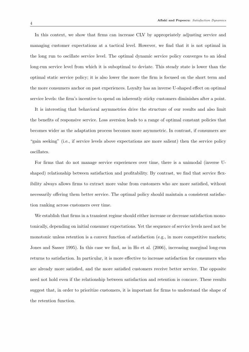
In this context, we show that firms can increase CLV by appropriately adjusting service and

managing customer expectations at a tactical level. However, we find that it is not optimal in

the long run to oscillate service level. The optimal dynamic service policy converges to an ideal

long-run service level from which it is suboptimal to deviate. This steady state is lower than the

optimal static service policy; it is also lower the more the firm is focused on the short term and

the more consumers anchor on past experiences. Loyalty has an inverse U-shaped effect on optimal

service levels: the firm’s incentive to spend on inherently sticky customers diminishes after a point.

It is interesting that behavioral asymmetries drive the structure of our results and also limit

the benefits of responsive service. Loss aversion leads to a range of optimal constant policies that

becomes wider as the adaptation process becomes more asymmetric. In contrast, if consumers are

“gain seeking” (i.e., if service levels above expectations are more salient) then the service policy

oscillates.

For firms that do not manage service experiences over time, there is a unimodal (inverse U-

shaped) relationship between satisfaction and profitability. By contrast, we find that service flex-

ibility always allows firms to extract more value from customers who are more satisfied, without

necessarily offering them better service. The optimal policy should maintain a consistent satisfac-

tion ranking across customers over time.

We establish that firms in a transient regime should either increase or decrease satisfaction mono-

tonically, depending on initial consumer expectations. Yet the sequence of service levels need not be

monotonic unless retention is a convex function of satisfaction (e.g., in more competitive markets;

Jones and Sasser 1995). In this case we find, as in Ho et al. (2006), increasing marginal long-run

returns to satisfaction. In particular, it is more effective to increase satisfaction for consumers who

are already more satisfied, and the more satisfied customers receive better service. The opposite

need not hold even if the relationship between satisfaction and retention is concave. These results

suggest that, in order to prioritize customers, it is important for firms to understand the shape of

the retention function.


The robust structure of a policy based on satisfaction suggests that firms should focus on satis-

faction, rather than service, as a metric for managing relationships over time. In sum, our results

show how service suppliers can leverage their customer-level data and service flexibility to increase

retention and improve long-term performance by gradually managing service expectations.

2. Related Literature and Customer Behavior Model

This section reviews related work and then develops our customer behavior model, which is based

on psychology and marketing literature.

2.1. Related Literature

Our work emerges from the interface of a relatively large literature on satisfaction and service-

relationship management in marketing, reviewed by Zeithaml (2000) and Rust and Chung (2006),

respectively, and the growing literature in behavioral operations; see Ferrer and Rocha e Oliveira

(2008) and Loch and Wu (2007) for reviews.

Several marketing frameworks capture the trade-off between cost and customer retention, includ-

ing the customer lifetime value (CLV) framework (Rust et al. 2004; Venkatesan and Kumar 2004),

the return on quality (ROQ) framework (Rust et al. 1995), and the customer equity framework

(Blattberg and Deighton 1996).

Few papers consider optimal investment decisions in customer satisfaction. Ho et al. (2006)

model customer purchases as a Poisson process whose rate depends on customer satisfaction, and

the probability p that a customer is satisfied in a given period is controlled by the firm. Focusing

on static policies, these authors find that customer value is increasing and convex in satisfaction.

However, their model neither captures the evolution of customer experiences over time nor its

endogenous effect on retention. Liu et al. (2007) consider the problem of inter-temporal allocation

of a limited capacity (sales-force effort) to a customer who forms adaptive expectations based on

prior service experiences. These expectations affect short-term profit but not retention. The focus

on allocating an exhaustible resource over a limited time period renders their model and insights

inherently different from ours.


There is a growing operations literature that examines endogenous models of demand in repeated

interaction settings. In this context, customers form adaptive expectations based on the firm’s past

policies, including pricing (Popescu and Wu 2007; Nasiry and Popescu 2009), capacity (Liu and

van Ryzin 2009), and quality (Caulkins et al. 2006). Closest to our work is that of Gaur and Park

(2007), who derive steady-state results in an oligopoly where loss-averse customers form adaptive

expectations about retailers’ fill rates. Their asymmetric adaptation model is similar to our model

in Section 7.1. These authors find that loss aversion leads to lower industry profits (consistent with

our findings) and higher service levels (an effect of strategic interaction).

In the service operations literature, Gans (2003) characterizes the firm’s optimal stationary

service policy in an oligopoly when customers respond in a Bayesian fashion to any change in service.

Our model is different in that it leverages the firm’s service flexibility by analyzing dynamic service

policies in the absence of strategic interactions. In our model, competition is captured indirectly,

through the retention function. In a duopoly setting, Hall and Porteus (2000) consider a finite-

horizon dynamic model where demand is a function of “service failures”, which are determined by

the firm’s investment in capacity. Their customers are purely reactive in their switching behavior,

with no memory of experiences prior to the current period. In contrast, our work endogenizes

retention by explicitly modeling customers’ evolution of satisfaction.

Two combined features distinguish our work from this literature. First, we draw on behavioral

theories—such as adaptive expectations and loss aversion—to endogenize retention based on past

service experiences in a dynamic service-satisfaction framework. Second, we go beyond steady-state

analysis to investigate the dynamics of customized service decisions over time, which are critical

for managing individual customer relationships.

2.2. The Customer Behavior Model

The effect of variations in service on customer lifetime value is more pronounced in B2B contexts

as well as “continuously provided services”, in which case revenue streams are closely tied with

retention. In such settings, customers dynamically adjust their perception of service quality based


on recent service encounters, and these perceptions ultimately determine repurchase behavior. This

section models the relationships among service, satisfaction, and retention based on evidence from

behavioral sciences and from a vast marketing literature on the antecedents and consequences of

satisfaction (see Anderson and Sullivan 1993).

2.2.1. The link between service and satisfaction. In the marketing literature, “customer

satisfaction” refers to a dynamic construct, formed after each service encounter (Bolton and Drew

1991a), as a function of the customer’s immediate perception of service and her service expectation

(see Tse and Wilton 1988 and the references therein).1 We assume that customer satisfaction reflects

previous experiences with the firm, which are used as a basis to form endogenous expectations about

what will happen in the next service encounter. Satisfaction is then updated based on perceived

service levels.

The most common model of satisfaction updating is an adaptive expectation model, where

satisfaction st+1 is a weighted average of past satisfaction st and current service xt. For simplicity

we assume that both service x and satisfaction s are measured in percentage terms: x, s ∈ [0,1].2

The following exponential smoothing model captures the essence of theoretical models on belief

formation (Hogarth and Einhorn 1992) and satisfaction (discussed below); it is also the simplest

model that renders the main insights from our framework:

st+1 = λst + (1−λ)xt. (1)

The adaptation parameter λ∈ [0,1) is the weight that the customer puts on prior experiences and

beliefs in order to update her satisfaction level. Customers with lower λ focus more on more recent

experiences; in particular, the satisfaction of the customers for whom λ= 0 is solely determined by

the most recent service experience. Exponential smoothing models have been used extensively to

1 Boulding et al. (1993) distinguish two types of expectations: will expectations, closely tied with the customer’sprevious experiences with the firm, refer to customer’s expectations about what will happen in the next serviceencounter; should expectations reflect normative beliefs about what service levels should be, based on exogenousvariables such as firm’s reputation, industry standards, and expert opinions. Our focus is on the endogenous effectsof the firm’s service decisions and hence on will expectations.

2 This allows us to capture a variety of service decisions, including the binary (service, no service) models typicallyused in the literature; in this case, x represents the fraction of time that service is offered over a given time period.


model adaptive expectations in an operational context (see, e.g., Caulkins et al. 2006; Gaur and

Park 2007; Liu et al. 2007; Popescu and Wu 2007).

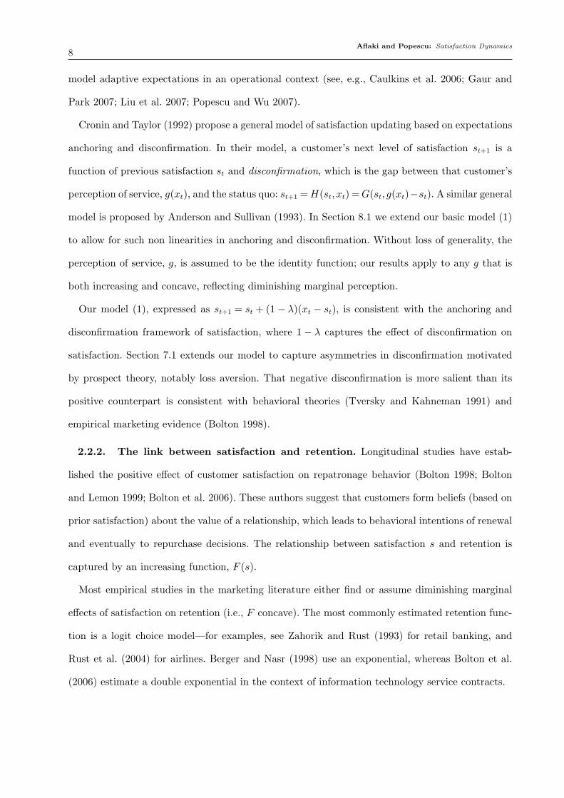
Cronin and Taylor (1992) propose a general model of satisfaction updating based on expectations

anchoring and disconfirmation. In their model, a customer’s next level of satisfaction st+1 is a

function of previous satisfaction st and disconfirmation, which is the gap between that customer’s

perception of service, g(xt), and the status quo: st+1 =H(st, xt) =G(st, g(xt)−st). A similar general

model is proposed by Anderson and Sullivan (1993). In Section 8.1 we extend our basic model (1)

to allow for such non linearities in anchoring and disconfirmation. Without loss of generality, the

perception of service, g, is assumed to be the identity function; our results apply to any g that is

both increasing and concave, reflecting diminishing marginal perception.

Our model (1), expressed as st+1 = st + (1− λ)(xt − st), is consistent with the anchoring and

disconfirmation framework of satisfaction, where 1− λ captures the effect of disconfirmation on

satisfaction. Section 7.1 extends our model to capture asymmetries in disconfirmation motivated

by prospect theory, notably loss aversion. That negative disconfirmation is more salient than its

positive counterpart is consistent with behavioral theories (Tversky and Kahneman 1991) and

empirical marketing evidence (Bolton 1998).

2.2.2. The link between satisfaction and retention. Longitudinal studies have estab-

lished the positive effect of customer satisfaction on repatronage behavior (Bolton 1998; Bolton

and Lemon 1999; Bolton et al. 2006). These authors suggest that customers form beliefs (based on

prior satisfaction) about the value of a relationship, which leads to behavioral intentions of renewal

and eventually to repurchase decisions. The relationship between satisfaction s and retention is

captured by an increasing function, F (s).

Most empirical studies in the marketing literature either find or assume diminishing marginal

effects of satisfaction on retention (i.e., F concave). The most commonly estimated retention func-

tion is a logit choice model—for examples, see Zahorik and Rust (1993) for retail banking, and

Rust et al. (2004) for airlines. Berger and Nasr (1998) use an exponential, whereas Bolton et al.

(2006) estimate a double exponential in the context of information technology service contracts.


Satisfaction (s)

Rete

ntio

n (F

)

local telephone

hospitals

personalcomputers

airlines

automobiles

1 2 3 4 5

Figure 1 “How the competitive environment affects the satisfaction–loyalty relationship” (Jones and Sasser

1995, p. 91).

Jones and Sasser (1995) argue that the marginal effect of satisfaction on loyalty need not be

diminishing and depends on the degree of market competition and customers’ switching costs.

Specifically, they find that F becomes more convex when the degree of competition in the market

increases, as illustrated in Figure 1 (replicated from their paper). They cite evidence from Xerox,

which found that increasing satisfaction ratings from 4 to 5 (on a 5-point scale) for its office

products customers increased the retention rate by a factor of 6, significantly more than for lower-

rating customers. Increasing marginal effects of satisfaction on loyalty (F convex) have also been

observed in the automotive industry (Mittal and Kamakura 2001).

We make no structural assumptions on the retention rate F beyond that it is increasing; that is,

more satisfied customers are more likely to renew, as evidenced in much of the marketing literature

(see Zeithaml 2000). In section 7.2 we relax this assumption by investigating an alternative model

in which value (and hence retention) is driven by disconfirmation, the gap between experience and

expectation: F (x− s). Such a model suggests that more satisfied customers are more difficult to

retain because they become more demanding, consistent with the treadmill effect (Brickman and

Campbell 1971) and with models of habituation (Baucells and Sarin 2010).

3. The Firm’s Problem

Marketing research suggests that “retaining customers is a far more profitable strategy than gain-

ing market share or reducing costs” (Zeithaml 2000), and goes so far as to recommend “separate

marketing plans — or even building two marketing organizations – for acquisition and retention


efforts” (Blattberg and Deighton 1996). Our model focuses on maximizing net present value from

the retention of existing customers (so-called defensive marketing), and does not consider acquisi-

tion and word of mouth-effects.

For simplicity of exposition we assume that, for each period during which the customer is active,

the revenue (or margin) is fixed and equal to P . So the short-term profit from offering service

level x is π(x) = P − c(x), where c is an increasing convex cost of service. This model is consistent

with service contracts in B2B and subscription services in B2C (e.g., insurance, information service

providers, lifestyle memberships, credit cards, telecom, cable/TV).

In broader contexts, satisfaction may affect customer spending (Seiders et al. 2005). In the

case of Harrah’s, for example, satisfaction may not influence a customer’s overall spending on

gambling, but it can affect the share of his gambling budget spent with the company (and not with

competitors). As discussed in Section 8.2, all our results extend without loss of generality to allow

for the effect of satisfaction on customer spending P = P (s)— or, more general short-term profit

models π(x, s) — as long as the marginal cost of service is increasing. The assumption of convex

costs, which is ubiquitous in the context of service operations, can be motivated by explicitly

deriving costs in various service delivery systems, such as queueing systems or inventory problems

(cf. Ho et al. 2006).

3.1. Dynamic Model

In our stylized model, the firm is fully informed about customer behavior (owing to extensive

customer-level data), and has the capability to adjust service based on this information. The

firm’s objective is to maximize the long-term value of each customer by dynamically adjusting the

customized service level xt, in response to the endogenous consumer behavior process described

in section 2.2. The main trade-off is between the short-term cost of providing high service and

the long-term benefit of increasing retention and future revenue streams. Under the exponential

smoothing model (1) for satisfaction updating, this problem can be formulated as a discounted

dynamic program with the following Bellman equation:

J(s) = maxx∈[0,1]

π(x) +βF (λs+ (1−λ)x)J(λs+ (1−λ)x). (2)


This is equivalent to an infinite horizon stochastic shortest path problem, with discount factor

β ∈ [0,1], representing how much the firm discounts future profits. Alternatively, β is a proxy for

the frequency of service encounters (the further away the next purchase is, the more heavily it is

discounted). Our model and results extend to capture non linear satisfaction formation mechanisms

as well as the effect of satisfaction on purchase frequency and customer spending (or short-term

profitability), as shown in Section 8.

Lemma 1. The value function J(·) is increasing, and P ≤ J(s)≤ P1−β for all s∈ [0,1].

Lemma 1 follows as a direct consequence of the satisfaction–retention relationship F being

increasing (Bolton 1998). This result shows that a firm with the flexibility to vary service level

optimally over time is always able to extract more value from customers who are ex ante more

satisfied, thereby realizing customers’ full profit potential. This is a benefit of service flexibility,

as the profitability relationship need not be monotone for firms that keep service and satisfaction

constant over time (Blattberg and Deighton 1996), as discussed in the next section.

3.2. Static Benchmark Model

If a firm does not have the flexibility to change service level x over time, then the long-term profit

from maintaining a constant service level x (consistent with customer expectations) is given by the

well-known CLV formula (Rust et al. 2004):

Π(x) =∞∑t=0

βtF t(x)π(x) =π(x)

1−βF (x)= π(x)L(x). (3)

We use L(x) = 1/(1− βF (x)) to denote the expected lifetime of the customer, given a constant

service level x; L(x) is increasing in x. If we assume unit demand in each period, then L(x) can

be interpreted as the expected total demand from the customer over her lifetime. The expected

customer lifetime value given a constant satisfaction level x, Π(x), is the product of the short-term

profit π(x) of each active customer and her expected lifetime L(x). Because π is decreasing and L

is increasing, Π is typically not monotone.

The marketing literature (see Rust et al. 1995) provides ample evidence of the diminishing

marginal returns to increasing satisfaction (i.e., that Π is concave), so Π has a unique maximizer s̄.


To guarantee uniqueness of optimal solutions throughout the paper, we make the following milder

assumption.

Assumption 1. c′(s)/L′(s) is strictly increasing in s.

Assumption 1 is satisfied for common parametric models used in the literature, such as logistic

F (x) = 1/(1 + exp(−αx)) or exponential F (x) = 1− exp(−αx) retention and for power cost c(x) =

x1+θ with θ≥ α. Other assumptions that guarantee uniqueness of optimal solutions throughout the

paper are strict concavity of Π or alternatively, strict quasi-concavity of Π and λπ+ (1−λ)Π.

Assumption 1 ensures that Π has a unique maximizer s̄, which is the optimal static service level.

In order to characterize this level, define the marginal cost per marginal customer lifetime as

C(x) =(c(x)L(x))′

L′(x)= c(x) + c′(x)

L(x)L′(x)

= c(x) + c′(x)1−βF (x)βF ′(x)

. (4)

Lemma 2. There exists a unique optimal static service level s̄ ∈ [0,1] that solves: (a) P =C(x)

as given by (4) when P ∈ [C(0),C(1)], (b) s̄= 1 for P ≥C(1), and (c) s̄= 0 for P ≤C(0).

Rewriting P =C(x) as (c(x)L(x))′ = (PL(x))′ reveals that the optimal static service level balances

the long-run marginal cost and marginal revenue of offering service, which is consistent with the

standard microeconomics insight. An implication of Lemma 2 is that Π is quasi-concave and, in

particular, non monotone for P ∈ [C(0),C(1)], consistent with marketing literature (Rust et al.

1995; Blattberg and Deighton 1996).

4. Long-Run Policy

Consider a firm that offers a constant service level st ≡ s̄ (as determined by Lemma 2) in each

period, so that customer expectations are anchored to s̄. Is it possible for the firm to extract more

profit in the long run from this customer by varying service? If so, how?

Figure 2 suggests that the firm can improve profits (by at least 10% relative to the static optimal

policy s̄= 0.7) simply by reducing the service quality in the first two periods and offering higher

service in the long run. Observe that this policy makes both the firm and the consumers better off

over the long run, though at the expense of a short-lived reduction in service. Alternatively, the


2 4 6 8 10 12 14 16 18 20

0.3

0.4

0.5

0.6

0.7

0.8

0.9

1

t

s t

+10%

+11%

Figure 2 The value of flexibility in service. F (s) = s0.9, c(x) = x2, λ= 0.8, β = 0.94, P = 1.

firm can obtain even higher profits (an 11% improvement) by adopting an oscillating, high–low

service policy; this is illustrated by the zigzag path in Figure 2.

The example indicates that firms can indeed do better by varying service, even if only temporarily.

It remains for us to establish whether these insights are robust and what the optimal service policy

actually looks like. In particular, the following questions should be addressed. (i) Is it optimal to

oscillate between high and low service in the long run, or is there an ideal long-run service level

for which the firm should aim? (ii) Is it always possible for the firm to improve profits by varying

service in the short run (as compared with implementing a constant service policy), and (iii) when

can the firm do so, while also providing better service to the customer in the long run? We provide

formal answers to these questions in what follows.

4.1. Steady State

This section characterizes an ideal long-run service level from which it is suboptimal to deviate.

By definition, s∗∗ is a steady state if the firm has no incentive to move away from it—that is if it

is a fixed point of the optimal service policy: x∗(s∗∗) = s∗∗, where x∗(·) is the policy that optimizes

(2). In other words, if customers’ satisfaction is in steady state, s∗∗, then it is optimal for the firm

to offer x= s∗∗ in each period.

Now consider the memory-adjusted marginal cost of service per marginal lifetime value:


C(s;λ) = c(s) +( λ

1−λ+L(s)

) c′(s)L′(s)

= c(s) + c′(s)(1−βF (s))(1−λβF (s))

β(1−λ)F ′(s), (5)

where C(s; 0) =C(s) as defined in (4). Because c(s) and L(s) are increasing, Assumption 1 guar-

antees that C(s;λ) is strictly increasing in s therefore, C =C(0, λ)<C(1, λ) =C.

The next result provides necessary conditions for a steady state to exist. Existence and global

stability are subsequently confirmed in Proposition 3.

Proposition 1. If problem (2) admits a steady state s∗∗, then this is unique and: (a) s∗∗ is

the unique solution of P = C(s;λ) if C < P < C; (b) s∗∗ = 1 if P ≥ C; (c) s∗∗ = 0 if P ≤ C.

Furthermore, s∗∗ is decreasing in λ and increasing in β and P .

Proposition 1 relates the firm’s long-run service policy to the firm’s strategic outlook as well as to

marketing (price) and operational (cost) factors. A firm with a short-term outlook puts less weight

β on future cash flows (e.g., β = 0 for a fully myopic firm), and provides lower long-run service and

satisfaction, because it focuses on (short-term) cost savings. All else equal, steeper costs or lower

prices reduce the firm’s incentive to invest in service and customer satisfaction.

Our results quantify the relationship between service level and contract price or customer spend-

ing, and they provide bounds on revenue indicating what it is worth for the firm to spend on

retention; see Figure 3. Some firms, such as the Ritz-Carlton, strive for full service and 100% satis-

faction across the board (Jones and Sasser 1995) whereas other businesses, such as Facebook and

Google’s Nexus phone, offer minimal customer service (Cachon and Terwiesch 2010). Our results

qualify the profitability of such practices by providing bounds on revenue for extreme policies to

be optimal in the long run. Specifically, below a relatively low price (P ≤C ≥ c(0)), the firm should

not increase its service expenditures (i.e., s∗∗ = 0). But for sufficiently high margins (P ≥C ≥ c(1)),

the firm should aim to maximize retention by offering full service over the long run.

Proposition 1 explains how the firm’s long-run policy is affected by customer behavior— in

particular by adaptation (or memory, λ) and loyalty (F ), as discussed next. The effect of behavioral

factors on profitability J is addressed in Section 6.2.


0 1 2 3 4 5 60

0.2

0.4

0.6

0.8

1

s**(P)

s(P)

P

Figure 3 Steady state s∗∗ and optimal static service s̄ as functions of price P , where F (s) = 1/(1 +

exp(−3s)), c(x) = x2 +x, λ= 0.5, β = 0.94; C = 1.15, C = 4.7.

The firm provides higher long-run satisfaction to customers who are more adaptive (or forgetful),

i.e. those who anchor on more recent experiences, captured by a lower λ. In particular, if satisfaction

is determined solely by the most recent service encounter (λ= 0), then the steady state coincides

with the optimal static service level: s∗∗(λ = 0) = s̄ = arg maxs∈[0,1] Π(s). In general, the steady-

state service level s∗∗(λ) is always lower than the static optimal policy s̄; see Figure 3. This follows

because C(s;λ) is increasing in λ, since s̄ solves P =C(s) =C(s; 0) and s∗∗ solves P =C(s;λ).

Remark 1. s∗∗ ≤ s̄.

In order to understand the effect of loyalty on the steady state, consider a parametric logit model

F (s;α) = 1/(1 + exp(−αs)), the most common retention model estimated in the literature. The

retention rate F (s;α) increases with α, which acts as a proxy for customer loyalty. Figure 4 shows

that the steady state is non monotone in α: it increases up to a certain point but then decreases.

This suggests that there is an “ideal” loyalty level beyond which the firm will treat the customer

as a captured audience and hence reduce costly investment in retention.

In this model, α also determines the degree of concavity of F , which is linked to the level of

competition in the market environment (as argued in Jones and Sasser 1995). This suggests that,

from the customers’ point of view, there is an optimal level of market competition that results

in the highest steady-state service level. These insights are partially consistent with Hall and

Porteus (2000), who find that loyalty decreases long-run service levels in an oligopoly. Our model

captures competitive effects implicitly, through customer choice, but does not account for strategic


0 2 4 6 8 10

s**

0

0.1

0.2

0.3

0.4

0.5

0.6

s0 0.2 0.4 0.6 0.8 1

F s

0.4

0.5

0.6

0.7

0.8

0.9

1.0

= 1

= 10

= 5

= 0

Figure 4 The effect of loyalty α on steady state service s∗∗ and retention F ; F (s;α) = 1/(1 + exp(−αs)), c(x) =

x2, λ= 0.5, β = 0.94.

interaction.

Corollary 1. The steady state s∗∗ of problem (2) maximizes over s∈ [0,1] the function:

W (s) = λπ(s) + (1−λ)Π(s). (6)

This result shows that an alternative to Assumption 1, which ensures uniqueness of the steady

state, is that W be strictly quasi-concave (in particular that Π be strictly concave). Corollary 1

suggests that in steady state the firm balances short term-profit (π) and long-term customer value

(Π), as weighed by customer memory λ, by solving λπ′(s) + (1− λ)Π′(s) = 0. From a technical

standpoint, W as defined in (6), is an important construct for problem (2) because it is a Lyapounov

function.3

4.2. Limited Flexibility

In Section 4.1 we characterized a unique service level s∗∗ from which it is suboptimal to deviate.

We now show that, unless s0 = s∗∗ (i) the firm can always do better by varying service in the short

run (first two periods); and, moreover, (ii) a policy can always be devised where both firm and

customer are better off in the long run, at the expense of a short disturbance in service. These

results validate the robustness of the example presented in Figure 2.

3 Specifically, W describes a “hill” that solutions to (2) are always climbing, with s∗∗ at the top, which ensures globalstability (see the proof of Proposition 3). In general, Lyapounov functions are hard to come by; “there is no wayother than unsystematic ingenuity to find them” (Stokey et al. 1989, p. 140).


The long-term expected customer profit associated with a given service path ℘= {xt, t≥ 1}, as a

function of the prior satisfaction level s0, is denoted J℘(s0). In particular, for the path xt ≡ x= s0

we have J℘(x) = Π(x).

Proposition 2. For any s0 6= s∗∗, there exists a service path ℘= {x1, x2, xt = s0, t≥ 3} that is

more profitable than the constant service path {xt = s0, t≥ 0}, i.e. J℘(s0)>Π(s0).

This result shows that, if expectations are not in steady state, then the firm can obtain higher

profits by varying service temporarily (over the first two periods). Moreover, the result extends for

strategic transitions to a prespecified service level x = xt, t ≥ 2. For all but finitely many values

x 6= s0, it is more profitable to vary service temporarily (so as to manage expectations in the

transition) than to shift directly from s0 to the new service level x. Smooth service downgrading

(or upgrading) is practiced in various industries, such as airlines (Cruz and Papadopoulos 2003).

Finally, we argue that both the firm and the customer can be better off over the long run if the

firm has the flexibility to temporarily vary service.

Corollary 2. For any initial customer expectation s0 6= s∗∗, there exists a service level x> s0

and a service path ℘(x) = {x0, x1, xt = x, t ≥ 2} that is more profitable than the constant service

path {xt = s0, t≥ 0}; that is J℘(x)(s0)>Π(s0).

Consider, for example, a firm that follows the optimal static service policy determined in Section

3.2 and offers a constant service level s̄. In this case, it is reasonable to assume that a customer’s

expectation of service is s0 = s̄. Proposition 2 shows that exploiting the behavioral effects of changes

in service on customer satisfaction and retention enables firms to improve customer profitability

by temporarily varying service. Moreover, Corollary 2 indicates that long-run win–win solutions

can be designed whereby the firm can obtain higher net present value than the best static policy

(Π(s̄)) and simultaneously offer better service (x> s̄= s0) to customers over the long run (albeit

at the cost of a temporary disturbance in service).


5. Transient Satisfaction Policy

In Section 4 we showed that the firm can benefit from varying service, either temporarily or in the

long run, when expectations are not in steady state. Naturally the question then arises as to what

is the best way to leverage service flexibility.

In this section we characterize the transient structure of the firm’s optimal policy. Our results

suggest that it is conceptually (and technically) more effective to focus on satisfaction, rather than

service, as a decision variable because doing so leads to unified, robust insights. Because the firm

is fully informed about the satisfaction updating process, deciding on a service level is equivalent

in our setting to choosing the next level of customer’s satisfaction.

Define π̄(r, s) = π( r−λs1−λ ); then, in terms of the variable st+1 = λst+(1−λ)xt, problem (2) becomes

J(st) = maxst+1∈s(st)

π̄(st+1, st) +βF (st+1)J(st+1). (7)

Here s(st) = [λst, λst + (1− λ)] is the feasible set of next-period satisfaction st+1 associated with

the constraint xt ∈ [0,1]. The optimal satisfaction policy s∗(·) solves (7) and satisfies s∗(s) = λr+

(1−λ)x∗(s) for the optimal service policy x∗(·), that solves (2). Technically, the advantage of this

model over its equivalent formulation (2) is that it avoids the complex interaction between state

and decision variables in the expected profit-to-go. Thus, supermodularity of the argument of the

Bellman equation (7) is ensured by concavity of short-term profits π, with no assumption on the

renewal rate F .

The following result establishes existence and global stability of the unique steady state deter-

mined by Proposition 1, and it characterizes the structure of the optimal transient policy.

Proposition 3. The optimal satisfaction policy s∗(·) is increasing. Moreover, the optimal sat-

isfaction path {s∗t} converges monotonically to the unique steady state s∗∗ characterized by Propo-

sition 1. The optimal service path {x∗t} also converges to the steady state s∗∗.

Proposition 3 shows that there does exist an ideal satisfaction level that the firm will deliver in the

long run, regardless of customers’ prior expectations. If initial expectations are not in steady state,


2 4 6 8 10 12 14 160

0.1

0.2

0.3

0.4

0.5

0.6

0.7

0.8

0.9

1Satisfaction Path

t0.2 0.4 0.6 0.8 1

0

0.2

0.4

0.6

0.8

1Satisfaction Policy

s

s** s**

Figure 5 (a) Optimal dynamic satisfaction paths st+1 = s∗(st) as a function of prior satisfaction s0; (b) optimal

satisfaction policy s∗(·) and steady state s∗∗; F (s) = 1/(1 + exp(−3s)), c(x) = x2, λ= 0.5, β = 0.94.

s0 6= s∗∗, then the firm benefits from adjusting service level and the optimal way of doing so induces

a monotone satisfaction path that converges to s∗∗. As illustrated in Figure 5, if customers have low

initial expectations, the firm will gradually increase satisfaction to s∗∗ by systematically offering

service above expectations; and the opposite holds if customers have high initial expectations.

Relative to a constant policy, which maintains service at current expectations, the optimal policy

increases expected lifetime for less satisfied customers by improving their service experience and

also capitalizes on short-term profits for more satisfied customers. The steady state balances the

marginal short-term cost of increasing satisfaction against the corresponding marginal expected

return over the long run.

Proposition 3 indicates that the service path will converge to the same steady state but makes

no statement regarding monotonicity of the service policy. Indeed, it is possible that the optimal

service policy is not increasing or even monotone. So even though it is optimal for the firm to

deliver higher satisfaction to ex ante more satisfied customers, they may not actually receive higher

service, as discussed in Section 6.1. Given the robust nature of insights concerning the satisfaction

(vs. service) policy, we conclude that firms should consider monitoring satisfaction rather than

service. The cost of doing so may not be an issue, given that “many companies routinely measure

customer satisfaction rather than service quality” (Rust et al. 1995).


6. Customer Value and Prioritization

Section 5 characterized the optimal satisfaction policy over the long run within a transient regime.

Firms can use this information to infer which customers are more valuable and benefit more from

an optimal dynamic service strategy. In particular, should customers who are more satisfied receive

higher service? Should the firm prioritize increasing satisfaction for more or less satisfied customers?

Which types of customers (e.g., more loyal, more adaptive) are more profitable for the firm? These

issues are addressed in this section.

6.1. Marginal Return on Satisfaction and Optimal Service Policy

Here we investigate the structure of the optimal service policy and the nature of marginal returns

to satisfaction as captured by the shape of the value function J . We argue that both depend on

the nature of customer loyalty—that is, the shape of the retention function F (see Section 2.2.2).

Proposition 4. If F (s) is convex, then the optimal service policy x∗(s) is increasing and the

value function J(s) is convex. The opposite need not hold when F (s) is concave.

Proposition 4 implies that more satisfied customers receive better service if satisfaction has an

increasing marginal impact on retention; this appears to be the case in more competitive industries

(Jones and Sasser 1995). The result is not robust when F is non convex or in particular, concave.

When F is concave, the optimal policy can be decreasing; that is, more satisfied customers actually

receive lower service although their overall satisfaction remains higher (see Figure 6). Concavity of

F, however, does not generally guarantee this result. Indeed, Figure 7 illustrates cases when F is

concave but x∗(·) is increasing.

Increasing marginal returns to satisfaction over the long run may seem to contradict conventional

wisdom (Rust et al. 1995). Yet, Ho et al. (2006) find that, for static policies, customer value can

be convex if costs are not too steep; they attribute this effect to a disaggregate view of customer

behavior in their model. Our result is not driven by cost but rather by the shape of the retention

function, which does not figure in their paper.


1 2 3 4 5 60

0.2

0.4

0.6

0.8

1Service and Satisfaction Paths

t0.2 0.4 0.6 0.8 1

0

0.2

0.4

0.6

0.8

1Service and Satisfaction Policies

s

xt

st

x*(s)

s*(s)

Figure 6 The optimal service policy and path can be decreasing, while the satisfaction policy and path are

increasing for F concave; F (s) = 1/(1 + exp(−5s)), c(x) = x2, λ= 0.5, β = 0.94, s0 = 0.3.

0 0.2 0.4 0.6 0.8 11

2

3

s

Cus

tom

er V

alue

0

0.2

0.4

0.6

0.8

1

Ser

vice

Pol

icy

0 0.2 0.4 0.6 0.8 12.5

3

3.5

4

s

Cus

tom

er V

alue

0

0.2

0.4

0.6

0.8

1

Ser

vice

Pol

icy

F(s)=s0.9 F(s)=1/(1+exp(-3s))

J(s) Convex J(s) Concave

J(s)

x*(s)

x*(s)

J(s)

Figure 7 Customer value J can be convex or concave and the optimal service policy x∗ can be increasing for F

concave; c(x) = x2, λ= 0.5, β = 0.94.

The controversial suggestion that firms may want to focus on (increasing satisfaction for) cus-

tomers who already are relatively more satisfied was advanced by Jones and Sasser (1995), who

suggested that such priorities should be determined by whether the retention rate is convex or

concave. Proposition 4 partially confirms their intuition for the case when F is convex. However,

in contrast to these authors, we find that firms may experience increasing marginal returns to

satisfaction even when the latter has a diminishing marginal effect on retention. An example is

illustrated in Figure 7, where J can be either convex or concave for F concave.

Intuition suggests that the shape of the value function J depends on the degree of concavity of

F . Characterizing this relationship analytically is difficult because of the multiplicative interaction

effects in the value-to-go (2) or (7), which make preservation of structural properties (e.g., con-


cavity) problematic. A sufficient condition for J(s) to be concave (resp. convex) and the optimal

service policy x∗(s) to be decreasing (resp. increasing) is the concavity (convexity) of (FJ)(s) (see

the proof of Proposition 4). This property is generally not preserved, however, since FJ may not

be concave even when both F and J are (increasing and) concave. Numerical results for parametric

logit, exponential, and power retention rates F suggest that, for sufficiently concave F , customer

value J (but not necessarily FJ) becomes concave and the optimal service policy may remain

increasing.

6.2. The Effect of Behavioral Parameters on the Value Function

A key premise of our work is that behavioral factors, such as customer loyalty and memory, affect

demand and profitability. Understanding these effects facilitates identifying the customer types

that are more valuable to the firm. Our results in Section 4.1 show that customers who adapt faster

(or are more forgetful) receive better service in the long run. But are these customers also more

valuable to the firm? What about customers who are more loyal? Do they remain more profitable

when they do not receive better service? (See Figure 4.)

Proposition 5. (a) The marginal effect of memory on the value function ddλJ(s;λ) is positive

for s > s∗∗(λ), negative for s < s∗∗(λ), and zero at s = s∗∗(λ). (b) If F (s;α) is increasing in the

loyalty parameter α, then J(s;α) is also increasing in α.

Part (a) states that the value function is locally monotone in the adaptation parameter λ but

that the direction of monotonicity depends on customer satisfaction. All else equal, the firm can

extract more value from satisfied customers when prior experiences are more salient (i.e., when

customers adjust their expectations more slowly). Empirical evidence suggests that “customers

who have many months’ experience with the organization weigh prior cumulative satisfaction more

heavily and new information (relatively) less heavily” (Bolton 1998). In this case, Proposition 5

suggests that, ceteris paribus, the focus should be on customers who have a longer history with the

firm if they are satisfied. Among the unsatisfied customers, the firm should focus on the recently

acquired ones because they are less anchored on past experiences and adapt faster. Figure 8(a)


s** JL S i C t V l

Customer�Value�(J)�RankingLong�run�Service Customer�Value

� ptation

(�)

Slow

Lowest�Value Highest�Value s0 high

�

Adap

yptation�( Slow

s0 low

�

Loyalty

Ada Fast

(b)

Low HighSatisfaction�(s0)

(a) (b)(a)

Figure 8 (a) Effect of customer adaptation speed on value depends on prior satisfaction s0; (b) Effect of adap-

tation and loyalty on service and customer value.

summarizes these insights, suggesting that ’old’ customers are the most valuable assets for the firm

if they are happy, but otherwise they may be the least valuable.

Part (b) of the proposition confirms the intuitive result that latent loyalty (higher α) is always

valuable to the firm. Recall, however, that more loyal customers may not receive better long-

run service, as illustrated in Figure 4 for F (x;α) = 1/(1 + exp(−αx)). The effect of behavioral

parameters (adaptation and loyalty) on customer value and long-run service is summarized in

Figure 8(b).

7. Asymmetries in Satisfaction and Renewal Processes

In this section we investigate, along lines that are consistent with prospect theory and marketing

evidence, the effect of behavioral asymmetries on adaptation and decision processes. We find that

these asymmetries, especially loss aversion, have important effects on the firm’s policy: (i) they

make constant service policies more prevalent, leading to a range of steady states; and (ii) optimal

service policies oscillate if the asymmetries are reversed.

These insights are preserved in an alternative retention model that is driven by disconfirmation,

in which customers react more to changes in satisfaction, rather than to absolute levels.

7.1. Loss Aversion and Satisfaction

Prospect theory postulates that decision makers code new information as gains or losses relative

to a status quo, a principle that applies to both decision and experience utility (Tversky and


Kahneman 1991; Kahneman et al. 1997). “Experienced utility” is the decision maker’s hedonic

value at the moment of experience which is captured by the concept of satisfaction in our model.

For both types of utility, a negative change from the status quo has a larger effect on value than

a positive change of the same magnitude. Generally known as loss aversion, this phenomenon has

received vast empirical support in the satisfaction literature (Boulding et al. 1993; Bolton 1998).

Consider the following asymmetric (kinked) satisfaction updating process:

sKt+1 ={sGt+1 = st + (1−λG)(xt− st) if xt ≥ st,sLt+1 = st + (1−λL)(xt− st) if xt < st,

(8)

where 1− λL > 1− λG expresses loss aversion. Such a kinked learning model is used by Gaur and

Park (2007) for consumers who form expectations about product availability (fill rate) and by

Nasiry and Popescu (2009) in a dynamic pricing context.

The Bellman equation for loss-averse adaptation can be written as follows:

JK(st) = maxxt∈[0,1]

π(xt) +βF (sKt+1)JK(sKt+1), (9)

where sKt+1 follows the transition dynamics (8). Let JL and JG denote the value functions of the

smooth problems (2) corresponding to λL and λG, respectively. Loss aversion implies that, by

Proposition 1, the corresponding steady states satisfy s∗∗L = s∗∗(λL) > s∗∗(λG) = s∗∗G . The kinked

adaptation process can be expressed as the minimum of two smooth exponential smoothing mech-

anisms, sKt+1 = min{sGt+1, sLt+1}, implying JK(s)≤min{JL(s), JG(s)} (see the Appendix). This sug-

gests that loss aversion—that is, the asymmetric effect of disappointing experiences relative to

pleasurable ones—has a negative effect on profitability. This is consistent with the findings in Gaur

and Park (2007).

Proposition 6. Assume that customers are loss averse (i.e., λL < λG). Then problem (9)

admits a range of steady states [s∗∗L , s∗∗G ]: starting from any s0 ∈ [s∗∗L , s∗∗G ], a constant service and

satisfaction path st = s0 is optimal. For s0 > s∗∗L , the satisfaction path st monotonically decreases

to s∗∗L and JK(s0) = JL(s0). For s0 < s∗∗G , the satisfaction path monotonically increases to s∗∗G and

JK(s0) = JG(s0). The service path converges to the same steady state as the corresponding satis-

faction path.


2 4 6 8 10 12 14 16 18 200.4

0.42

0.44

0.46

0.48

0.5

0.52

0.54

0.56

0.58

Satisfaction Path

t

Figure 9 The optimal satisfaction path oscillates for gain-seeking customers; F (s) = 1/(1 + exp(−3s)), c(x) =

x2, λG = 0.4, λL = 0.6, β = 0.94, P = 1.

Adding loss aversion to the model does not affect the structure of the transient policy, but it does

widen the set of steady states and so makes constant service policies more prevalent. Intuitively, the

firm has less leverage to improve perception when customers anchor more on negative experiences.

Technically, this is due to the kink in satisfaction updating.

For completeness, we briefly consider here the case where customers are “gain seeking” (i.e.,

λG < λL). This means that service experiences above expectations (positive disconfirmation) are

more salient than those below expectations (negative disconfirmation). Bolton et al. (2000) find

evidence that members of loyalty rewards programs tend to discount or overlook negative service

experiences. In this case, we find that no interior steady state exists. Under a high–low policy, the

firm benefits in the long-run by manipulating customer satisfaction and their expectations. The

benefits to the firm in this case are attributable to the positive net effect of increasing service and

then decreasing it back.

Proposition 7. If λL > λG then problem (9) admits no interior steady state. If, moreover,

C(0;λG)<P <C(1;λL), then any optimal service path oscillates.

7.2. Renewal Is Driven by Disconfirmation

The results so far have been based on a model where more satisfied customers are more likely to

renew; this assumption has the widest empirical support in the marketing literature. One could


argue, however, that more satisfied customers also have higher expectations and thus are more

likely to react negatively to lower service quality than those who expect less. This section considers

such a model where retention F depends only on disconfirmation, x− s, or the perceived gain or

loss relative to expectations. This model is a good proxy for cases when customers react more to

changes in service.

Evidence that disconfirmation is a better predictor of retention, than is customer satisfaction,

may be found, for example, in Bolton and Drew (1991b). The key difference from our previous

models is that here customers with higher expectations are less likely to renew. Intuitively, they

become harder to please as they grow accustomed to better service owing to the satisfaction

treadmill effect. Indeed, our model is consistent with the treadmill effect (Brickman and Campbell

1971), and habituation models (Baucells and Sarin 2010).

Loss aversion in customer’s decision process suggests that a perceived downgrade in service (neg-

ative disconfirmation) has a stronger impact on retention than a perceived improvement (positive

disconfirmation) of the same magnitude. Formally, we model the kinked retention rate as

FK(x− s) ={F (δL(x− s)) if x< s,F (δG(x− s)) if x≥ s, (10)

where δL > δG captures loss aversion. The corresponding Bellman equation is

JK(s) = maxx∈[0,1]

π(x) +βFK(x− s)JK(λs+ (1−λ)x). (11)

Lemma 3. JK(s) is decreasing in s. Moreover, if F is convex then JK is also convex.

This result is in sharp contrast with Lemma 1. If retention is driven by the gap between experience

and expectation, then customers who are more satisfied require higher maintenance, and this makes

them less profitable in the long run. However, the rest of our insights are preserved under this

conceptually and structurally different model.

Proposition 8. If customers are loss averse in their renewal decisions (i.e., δL ≥ δG) then

problem (11) admits a range of steady states [s∗∗(δG), s∗∗(δL)], where s∗∗(δ) solves

(1−λβF (0))π′(s) +βδF ′(0)π(s) = 0. (12)


If s0 > s∗∗(δL) then the optimal satisfaction path decreases to s∗∗(δL), and if s0 < s

∗∗(δG), then the

optimal satisfaction path increases to s∗∗(δG). If δL < δG, then no steady state exists.

8. Extensions: Alternative Satisfaction and Revenue Models

We now show that the main insights in this paper are robust when allowing for non linearity in the

satisfaction updating process as well as for alternative revenue models that account for the effect

of satisfaction on spending, purchase frequency, and social social planning objectives.

8.1. Non Linear Models of Satisfaction

Our results can be extended to account for general nonlinear effects in the satisfaction updating

process, st+1 =G(st, xt− st) =H(xt, st), as long as this satisfies the following assumption.

Assumption 2. (a) H(x, s) is increasing in x and s, and H(s, s) = s; (b) H11(x, s) ≤ 0; (c)

H12(x, s)≥ 0; (d) H22(s, s)≥ 0.

For convenience, partial derivatives are here denoted by corresponding subscripts. Part (a) states

that all else equal, both service level and ex ante satisfaction have a positive effect on ex post

satisfaction; this is consistent with empirical evidence (Oliver and DeSarbo 1988). In particular,

it suggests that the absolute effect of satisfaction dominates the effect of disconfirmation x− s;

the opposite effect was captured in Section 7.2. Satisfaction does not change if service remains

constant, H(s, s) = s, while controlling for exogenous effects on satisfaction. Diminishing marginal

sensitivity to service, (b), is a natural assumption. Part (c) and part (d) are technical conditions

stating that more satisfied customers are more sensitive to a change in service and to a change in

satisfaction, respectively. To the best of our knowledge, these hypotheses have not yet been tested

in the literature.

Assumption 2 is satisfied, for example, for an exponential smoothing model in which the weight

attached to the current experience depends on the current service level: H(x, s) = λ(x)s+ (1−

λ(x))x, provided that λ(x) is increasing and has a bound on its curvature, λ′(x)≥ |λ′′(x)|/2 (as

for, e.g., λ(x) = x, ex−1, and 1−e−x). In this model, lower service is more salient in memory— that


is, the lesser the current experience, the more it weighs on satisfaction. Section 7.1 described a

model in which experiences below expectations are more salient than those above expectations.

The Bellman equation corresponding to this problem is:

J(s) = maxx∈[0,1]

π(x) +βF (H(x, s))J(H(x, s)). (13)

Proposition 3 extends under this general adaptation process by replacing λ with λ(s) =H2(s, s),

the derivative of H(x, s) with respect to s, evaluated at x= s. In particular, for the exponential

smoothing model (1), we recover precisely λ(s) = λ.

Proposition 9. Under Assumption 2, the results in Proposition 1, Proposition 3 and Corollary

1 apply to model (13) once we redefine C(s;λ(s)) = c(s) +( λ(s)

1−λ(s)+L(s)

) c′(s)L′(s)

. In particular,

the corresponding steady state solves: λ(s)π′(s) + (1−λ(s))Π′(s) = 0.

We find it interesting that the steady state depends on the service–satisfaction relationship

only via λ(s), the marginal effect of expectations on satisfaction, when service is aligned with

expectations.

8.2. Alternative Profit Models

Our structural results are essentially driven by the concavity of the short-term profits π (supermod-

ularity of π̄), with no assumption on the retention function except monotonicity. This allows one to

extend the application of our insights to more complex revenue models, which capture the effect of

satisfaction on customer spending and purchase frequency, and also to nonprofit and public-service

contexts.

Satisfaction affects purchase frequency. Our structural results extend to capture the effect

of satisfaction on purchase frequency. Technically, this is equivalent to replacing β with βν(st+1) in

problem (7). Practical evidence suggests that more satisfied customers increase their frequency of

purchase (Sharma et al. 1999); in other words, ν(·) is decreasing. This transformation has no effect

on supermodularity of (7)’s argument, implying that our monotonicity and convergence results

hold without any additional assumptions on ν(·).


Satisfaction affects spending. Our results also extend for a general model π(x, s) where the

firm’s instant profit is a function of the offered service and satisfaction level, provided that π(x, s)

is supermodular and concave in service x. This holds, for example, if more satisfied customers are

more sensitive to changes in service, or if the marginal cost of serving them is lower. In particular,

this condition holds if customer spending P (s) is increasing in satisfaction but unaffected by current

service x; whereas convex costs depend only on current service c(x), so π(x, s) = P (s)− c(x).

Public services. In particular, consider a model in which the firm’s objective has a social

component: P (·) = (1−w)P +wS(·). Here w ∈ [0,1] is the weight that the firm puts on consumer

surplus, which is an increasing concave function of service S(x) or, alternatively, of satisfaction

S(s). As w→ 1, this becomes a public-services problem for a social planner who cares only about

customer surplus and not profit. All our results extend in this context. Moreover, customer sat-

isfaction increases as the firm puts more weight on consumer surplus (i.e., s∗∗(w) and s∗(w) are

increasing in w). In particular, a profit-focused monopolist (w= 0) will satisfy customers less than

a public planner with the same cost structure. But if social concerns are of major importance to

the firm and if the marginal social benefits of full satisfaction exceed marginal costs (specifically,

if w≥ c′(1)/S′(1)), then it is easy to see that offering full service is optimal, x∗ ≡ 1.

9. Conclusions

We relied on behavioral theories to develop a dynamic programming model of using responsive

service strategies to manage satisfaction over time in a customer relationship. In this context, we

showed that firms can extract more value in the long run by gradually managing service experiences

and expectations over time towards an “ideal” steady-state service level from which it is suboptimal

to deviate. Interestingly, behavioral asymmetries (such as loss aversion) drive the structure of

optimal long-run policies by ensuring convergence and increasing the prevalence of constant service

policies. Indeed, the more customers are averse to service downgrades, the wider is the range of

optimal constant service policies offered by the firm and the lower are its profits.

Our results provide insight into how firms with responsive service capabilities can use customer-

level information—such as prior satisfaction, loyalty, and adaptation—to prioritize customers in


terms of value and customized service. The relationships between various behavioral factors and

the firm’s policy and profits are summarized in Table 1.

More loyal customers are more valuable, but they may not receive better service if they are

inherently too sticky. Our model predicts a unimodal relationship between loyalty and service.

From the customers’ perspective, this means that there exists an ideal, intermediate level of loyalty

(driven, e.g., by switching costs or the level of market competition) that fetches the best service.

The firm offers less service in the long run to less adaptive customers, such as those with a longer

history; these are more profitable than customers who focus on recent experiences, but only if they

are sufficiently satisfied.

We find that the firm can always extract more value from more satisfied customers if they are

also more likely to renew. This is a direct benefit of service flexibility that would not be realized

if firms were constrained to maintain the same service level, or if renewal is mainly driven by

disconfirmation. The optimal policy preserves satisfaction ranking: ex ante more satisfied customers

remain more satisfied. However, they receive better service only if there are increasing marginal

returns to satisfaction. Contrary to existing predictions (Jones and Sasser 1995), this may be the

case even if satisfaction has diminishing marginal effects on retention.

Table 1 Effects of Consumer Behavior on Policy and Value

Behavioral Long-run Service Customer ValueFactor (steady state s∗∗) (J)Loyalty (α) Inverse U-shape Increasing

Adaptation (λ) Increasing Increasing for high s0;decreasing for low s0

Loss aversion Expands range Decreasing(ρ= λG/λL > 1) (oscillates if ρ< 1)

Initial satisfaction/ No effect Depends on what drives renewal:Expectation (s0) increasing, if satisfaction;

decreasing, if disconfirmation.

This paper is a first step toward capturing behavioral effects of service dynamics in a business

relationship. We have therefore strived for parsimony in developing the simplest stylized model


capable of transmitting the main insights from this framework. Ample opportunities exist for

future research to extend this model and address its limitations from an operational, marketing, or

economic perspective—for example, by incorporating strategic interaction, customer heterogeneity

and fairness perceptions, acquisition and network effects, and/or richer operational service struc-

tures. For expository purposes, we cast our model and results in the context of managing service

relationships. However, our setup can be expanded to broader contexts, such as employee retention,

effort and quality management.

References

Anderson, E. W., M. W. Sullivan. 1993. The antecedents and consequences of customer satisfaction for firms.

Marketing Science 12(2) 125–143.

Baucells, M., R. K. Sarin. 2010. Predicting Utility Under Satiation and Habit Formation. Management

Science 56(2) 286–301.

Berger, P. D., N. I. Nasr. 1998. Customer lifetime value: Marketing models and applications. Journal of

Interactive Marketing 12(1) 17–30.

Bitran, G. R., J. C. Ferrer, P. Rocha Oliveira. 2008. Managing customer experiences: Perspectives on the

temporal aspects of service encounters. Manufacturing & Service Operations Management 10(1) 61.

Blattberg, R.C., J. Deighton. 1996. Manage marketing by the customer equity test. Harvard Business Review

74 136–145.

Bolton, R. N. 1998. A dynamic model of the duration of the customer’s relationship with a continuous

service provider: The role of satisfaction. Marketing Science 17(1) 45.

Bolton, R. N., J. H. Drew. 1991a. A multistage model of customers’ assessments of service quality and value.

Journal of Consumer Research 17(4) 375–384.

Bolton, R. N., J.H. Drew. 1991b. A longitudinal analysis of the impact of service changes on customer

attitudes. The Journal of Marketing 1–9.

Bolton, R. N., P.K. Kannan, M.D. Bramlett. 2000. Implications of loyalty program membership and service

experiences for customer retention and value. Journal of the Academy of Marketing Science 28(1)

95–108.


Bolton, R. N., K. N. Lemon, M. D. Bramlett. 2006. The effect of service experiences over time on a supplier’s

retention of business customers. Management Science 52(12) 1811–1823.

Bolton, R. N., K.N. Lemon. 1999. A dynamic model of customers’ usage of services: usage as an antecedent

and consequence of satisfaction. Journal of Marketing Research 36(2) 171–186.

Boulding, W., A. Kalra, R. Staelin, V. A. Zeithaml. 1993. A dynamic process model of service quality: From

expectations to behavioral intentions. Journal of Marketing Research 30(1) 7–27.

Brickman, P., D.T. Campbell. 1971. Hedonic relativism and planning the good society. Adaptation level

theory: A symposium. Academic Press, 287–302.

Cachon, G., C. Terwiesch. 2010. Death to facebook a self service nightmare. Matching Supply with Demand

- Current events and issues in Operations Management URL http://mswd.wordpress.com/2010/01/

13/death-to-facebook-a-self-service-nightmare/.

Caulkins, J.P., G. Feichtinger, J. Haunschmied, G. Tragler. 2006. Quality cycles and the strategic manipu-

lation of value. Operations Research 54(4) 666–677.

Chase, R.B., S. Dasu. 2001. Want to perfect your company’s service? use behavioral science. Harvard

Business Review 79(6) 78–84.

Cronin, J. J., S. A. Taylor. 1992. Measuring service quality: a reexamination and extension. Journal of

Marketing 56(3) 55–68.

Cruz, A., L. Papadopoulos. 2003. The Evolution of the Airline Industry and Impact on Passenger Behaviour.

Passenger behaviour 32.

DeVine, J., K. Gilson. 2010. Using behavioral science to improve the customer experience. McKinsey

Quarterly February.

Ferrer, G. R. B. J. C., P. Rocha e Oliveira. 2008. Managing Customer Experiences: Perspectives on the

Temporal Aspects of Service Encounters. Manufacturing and Service Operations Management 10(1).

Gans, N. 2003. Customer loyalty and supplier quality competition. Management Science 48(2) 207–221.

Gaur, V., Y. Park. 2007. Asymmetric consumer learning and inventory competition. Management Science

53(2) 227.

Hall, J., E. Porteus. 2000. Customer service competition in capacitated systems. Manufacturing & Service

Operations Management 2(2) 144–165.


Ho, T., Y. H. Park, Y. P. Zhou. 2006. Incorporating Satisfaction into Customer Value Analysis: Optimal

Investment in Lifetime Value. Marketing Science 25(3) 260 – 277.

Hogarth, R. M., H. J. Einhorn. 1992. Order effects in belief updating: The belief-adjustment model. Cognitive

Psychology 24(1) 1–55.

Jones, T. O., W. E. Sasser. 1995. Why satisfied customers defect. Harvard Business Review 73(6) 88–91.

Kahneman, D., P. P. Wakker, R. Sarin. 1997. Back to bentham? explorations of experienced utility. Quarterly

Journal of Economics 112(2) 375.

Liu, B. S. C., N. C. Petruzzi, D. Sudharshan. 2007. A service effort allocation model for assessing customer

lifetime value in service marketing. Journal of Services Marketing 21 24–45.

Liu, Q., G. van Ryzin. 2009. Strategic capacity rationing when customers learn. Working paper, Columbia

University .

Loch, Ch., Y. Wu. 2007. Behavioral operations management. Foundations and Trends in Technology,

Information and Operations Management 1(3).

Mittal, V., W. A. Kamakura. 2001. Satisfaction, repurchase intent, and repurchase behavior: Investigating

the moderating effect of customer characteristics. Journal of Marketing Research 38(1) 131–142.

Nasiry, J., I. Popescu. 2009. Dynamic pricing with asymmetric consumer learning. INSEAD working paper .

Oliver, R. L., W. S. DeSarbo. 1988. Response determinants in satisfaction judgments. The Journal of

Consumer Research 14(4) 495–507.

Popescu, I., Y. Wu. 2007. Dynamic pricing strategies with reference effects. Operations Research 55(3) 413.

Rust, R. T., T. S. Chung. 2006. Marketing models of service and relationships. Marketing Science 25(6)

560–580.

Rust, R. T., K. N. Lemon, V. A. Zeithaml. 2004. Return on marketing: Using customer equity to focus

marketing strategy. Journal of Marketing 68(1) 109–127.

Rust, R. T., A. J. Zahorik, T. L. Keiningham. 1995. Return on quality (roq): Making service quality

financially accountable. The Journal of Marketing 59(2) 58–70.

Seiders, K., G. B. Voss, D. Grewal, A. L. Godfrey. 2005. Do satisfied customers buy more? examining

moderating influences in a retailing context. Journal of Marketing 69(4) 26–43.


Sharma, S., R. W. Niedrich, G. Dobbins. 1999. A framework for monitoring customer satisfaction: An

empirical illustration. Industrial Marketing Management 28(3) 231 – 243.

Stokey, N.L., R.E. Lucas, E.C. Prescott. 1989. Recursive methods in economic dynamics. Harvard University

Press.

Topkis, D. M. 1998. Supermodularity and complementarity . Princeton University Press.

Tse, D. K., P. C. Wilton. 1988. Models of consumer satisfaction formation: an extension. Journal of Marketing

Research 25(2) 204–212.

Tversky, A., D. Kahneman. 1991. Loss aversion in riskless choice: A reference-dependent model. The

Quarterly Journal of Economics 106(4) 1039–1061.

Venkatesan, R., V. Kumar. 2004. A customer lifetime value framework for customer selection and resource

allocation strategy. Journal of Marketing 106–125.

Zahorik, A. J., R. T. Rust. 1993. Customer satisfaction, customer retention, and market share. Journal of

Retailing 69(2) 103–125.

Zeithaml, V. A. 2000. Service quality, profitability, and the economic worth of customers: What we know

and what we need to learn. Journal of the Academy of Marketing Science 28(1) 67.

Appendix: Proofs

Proof of Lemma 1. Monotonicity of the value function holds because F (λs+(1−λ)x) is increas-

ing in x. Monotonicity is preserved by induction for the corresponding finite-horizon model and

then at the limit for our infinite-horizon formulation. The firm can at least extract P from the

customer by offering {xt ≡ 0}, so P ≤ J(s). An upper bound on customer value is obtained if the

customer never defects and the firm offers no added service, so J(s)≤∑∞

t=0 βtP = P

1−β .

Proof of Lemma 2. Assumption 1 guarantees that Π is unimodal, so its maximizer is unique.

We write the first-order condition with respect to x to obtain, after rearrangement, P = C(x).

By Assumption 1, C(x) is increasing and so C(0)<C(1). The rest of the result follows from the

unimodality of Π.

Proof of Proposition 1. (a) An interior steady state is given by the following Euler equation:


∂

∂st+1

{π(st+1−λst

1−λ

)+βF (st+1)

(π(st+2−λst+1

1−λ

)+βF (st+2)Π(st+2)

)}st=st+1=st+2=s

= 0.

(14)

Defining W (s) = λπ(s) + (1−λ)Π(s), we can rewrite (14) as

W ′(s) = (1−λ)βF ′(s)(P −C(s;λ)) = 0, (15)

which is equivalent to P =C(s;λ). Under Assumption 1, C(s;λ) is increasing and so the solution

to P = C(s;λ) is unique if it exists. Strict quasi-concavity of W (or strict concavity of Π) is also

sufficient for this.

It remains to show that (i) if P > C then s∗∗ = 0 cannot be a steady state; and (ii) if P < C

then s∗∗ = 1 cannot be steady state. For this we show that, starting from s0 = 0 (resp. s0 = 1), the

corresponding constant satisfaction paths with profits Π(0) (resp. Π(1)), are suboptimal.

(i) Consider the service path ℘0(δ) = {x1 = δ, xt = 0, t≥ 2}, and let J℘0(δ)(0) denote the corre-

sponding discounted profit starting at s0 = 0. We then have

limδ→0+

J℘0(δ)(0)−Π(0)δ

≥ limδ→0+

1δ

(J℘0(δ)(0)−π(0) +β(F ((1−λ)δ)−F (0))π(0)

)= π′(0) +β(1−λ)F ′(0)π(0)

= [1−βF (0)]2W ′(0)> 0, (16)

where the last inequality holds because P >C implies W ′(0)> 0.

(ii) Similarly, consider the service path ℘1(δ) = {x1 = 1−δ, xt = 1, t≥ 2} and let J℘1(δ)(1) denote

the corresponding profit starting at s0 = 1. Then

J℘1(δ)(1) = π(1− δ) +βπ(1)∞∑k=0

βkF (1− δλk(1−λ)). (17)

Therefore,

limδ→0+

J℘1(δ)(1)−Π(1)δ

= limδ→0+

1δ

(π(1− δ)−π(1) +βπ(1)

∞∑k=0

βk(F (1− δλk(1−λ))−F (1)))

= −π′(1)−β(1−λ)π(1)F ′(1)∞∑k=0

βkλk


= −π′(1)− β(1−λ)1−λβ

F ′(1)π(1)

> −π′(1)− β(1−λ)(1−λβ)(1−β)

F ′(1)π(1)

= − β(1−λ)(1−λβ)(1−β)

F ′(1)(P −P )> 0. (18)

The last inequality holds because P < P by definition. Hence, starting from s0 = 1, a profitable

deviation from the constant satisfaction path {st ≡ 1} exists and so s∗∗ = 1 cannot be a steady

state.

Moreover, C(s;λ) is decreasing in β because

∂C(s;λ)∂β

=−(1−λβ2[F (r)]2)c′(r)β(1−λ)F ′(r)

≤ 0.

Finally, since C(s;λ) is increasing in s and decreasing in β and since s∗∗ solves P = C(s;λ), it

follows that s∗∗ is increasing in β.

Proof of Corollary 1. This follows directly from the proof of Proposition 1.

Proof of Proposition 2. For any s0 ∈ (0,1), consider the variational path ℘(ε) = {x1 = s0 +

ε, x2 = s0 − λε, xt = s0, t ≥ 3}. We show that, for any initial expectation s0 6= s∗∗, there exists

|ε| ≤min{s0,1− s0} such that at least one of the feasible paths ℘(ε) or ℘(−ε) is more profitable

than the constant path st ≡ s0; that is, Π(s0)<max{J℘(ε)(s0), J℘(−ε)(s0)}.

It is easy to verify that under ℘(ε) we have s2 = s0 for any feasible ε (i.e., |ε| ≤min{s0,1− s0}),

which implies that

J℘(ε)(s0) = π(s0 + ε) +βF (s0 + (1−λ)ε)(π(s0−λε) +βF (s0)Π(s0)

). (19)

For ε > 0 we use Π(s0) = π(s0) +βF (s0)(π(s0) +βF (s0)Π(s0)

)to obtain

limε→0+

J℘(ε)(s0)−Π(s0)ε

= β(1−λ)F ′(s0)(π(s0) +βF (s0)Π(s0)

)+ (1−λβF (s0))π′(s0) (20)

= β(1−λ)F ′(s0)Π(s0) + (1−λβF (s0))π′(s0) (21)

= (1−βF (s0))W ′(s0). (22)


Similarly, using (19) for ℘(−ε), we obtain

limε→0+

J℘(−ε)(s0)−Π(s0)ε

=−(1−βF (s0))W ′(s0). (23)

The result follows because, by Assumption 1, W ′(s0) 6= 0 for s0 6= s∗∗.

Proof of Corollary 2. By Proposition 2, for any s0 6= s∗∗ there exist x0 and x1 such that

J(s0;x0, x1, s0)>Π(s0), where J(s0;x0, x1, x) is the value of the path {x0, x1, xt = x, t≥ 2} starting

at s0. The result then follows because J(s0;x0, x1, x) is continuous in x.

Proof of Proposition 3. By the concavity of π(·), the term on the right-hand side of the

Bellman equation (7) is supermodular in (st+1, st). Furthermore, the feasible sets s(st) are ascending

in st; that is, for any st ≤ s′t, r ∈ s(st), and r′ ∈ r(s′t) we have min(r, r′)∈ s(st) and max(r, r′)∈ s(s′t).

Therefore, by Topkis’s theorem (Topkis 1998, Thm. 2.8.2), the policy function s∗(·) is increasing on

[0,1]. It follows that s∗(·) must have a fixed point, s∗∗ = s∗(s∗∗), which is a steady state of problem

(7).

Moreover, monotonicity of s∗(·) implies that the state path {s∗t} is monotone (by induction),

and because the feasible set s(·) is compact, {s∗t} must converge to a steady state. Hence a steady

state exists, and by Proposition 1 it is unique. Finally, in steady state s∗∗ = λs∗∗ + (1 − λ)x∗∗,

so s∗∗ = x∗∗. In particular, because the satisfaction paths converge monotonically to s∗∗ (which

maximizes the unimodal function W ), it follows that W is a Lyapounov for our problem.

Proof of Proposition 4. The result holds because convexity is preserved by maximization and

limits. Indeed, if F (s) is convex, it follows by induction that the corresponding finite horizon value

function is also convex. By value iteration, we can take limits to obtain that the infinite horizon

value function J(s) is convex, so V (s) = F (s)J(s) is convex.

We further show that V convex (resp. concave) is sufficient for the service policy to be increasing

(decreasing) and the value function J to be convex (concave), confirming the statement at the

end of Section 6.1. Now, V convex (concave) is equivalent to the argument on the right-hand side

of the Bellman equation, Q(x, s) = π(x) + βV (λs+ (1− λ)x), being supermodular (submodular);

Monotonicity of the optimal policy then follows by Topkis’s theorem. Moreover, V convex implies


that Q(x, s) is convex in s, so J is convex. On the other hand, V concave implies that Q(x, s) is

jointly concave, so J is concave.

Proof of Proposition 5. For a given s0, consider the optimal service path st+1 = s∗(st) for all

t. By the envelope theorem, for all t we have

∂

∂λJ(st;λ) =

st+1− st(1−λ)2

π′(st+1−λst

1−λ

)+βF (st+1)

∂

∂λJ(st+1;λ). (24)

In particular, at steady state s0 = s∗∗(λ) = st we have (1−βF (s)) ∂∂λJ(s;λ)|s=s∗∗ = 0, which implies

the stated result. For s0 ≥ s∗∗(λ), by Proposition 3 the optimal satisfaction path is decreasing,

st+1 ≤ st for all t, so the first term in the right-hand side of (24) is positive. Thus, for any t > 0,

we have

∂

∂λJ(s0;λ) ≥ βF (s1)

∂

∂λJ(s1;λ) (25)

≥ β2F (s1)F (s2)∂

∂λJ(s2;λ)≥ · · · (26)

≥ limt→∞

βt

(t∏i=1

F (si)

)∂

∂λJ(st;λ) = 0. (27)

The last derivative is bounded as n→∞ because st→ s∗∗(λ) (Proposition 3). The case s0 ≤ s∗∗(λ)

is proved similarly.

Proof of Proposition 6. We transform problem (9) to obtain

JK(st) = maxsKt+1∈s(st)

π(sKt+1−λst

1−λ

)+βF (sKt+1)J

K(sKt+1). (28)

For any θ ∈ [0,1], let (Pθ) denote problem (28) where sθt+1 = θsGt+1 + (1− θ)sLt+1. This is equivalent

to a smooth model (7) with λθ = θλG + (1− θ)λL. Let Jθ and s∗∗θ denote (respectively) the value

function and the steady state of this problem. In particular, s∗∗θ=0 = s∗∗L and s∗∗θ=1 = s∗∗G .

Lemma 4. (a) JK(s) ≤ Jθ(s) for all s. (b) If s∗∗θ is a steady state for (Pθ), then it is also a

steady state for problem (28).

Proof of Lemma 4. (a) The claim follows from sθt+1 = θsGt+1 + (1− θ)sLt+1 ≥min{sGt+1, sLt+1}= sKt+1,

by induction on the finite-horizon versions of the corresponding problems, and then using value


iteration. (b) Starting from s∗∗θ , a constant satisfaction path is optimal for (Pθ). This path is feasible

for our kinked problem (28) and achieves the same value JK(s∗∗θ ) = Jθ(s∗∗θ ). Therefore, using part

(a) of Lemma 4, the constant path s∗∗θ must be optimal for problem (28) and so s∗∗θ is also a steady

state for this problem. �

By Proposition (3), if we start from s0 > s∗∗θ=0 = s∗∗L then the optimal satisfaction path in (PL)

decreases to s∗∗L . This path is feasible for problem (28) and gives the same value in both problems.

Because JL(s)≥ JK(s), for all s, the optimal path for (PL) is also optimal for problem (28). The

case s0 < s∗∗θ=1 = s∗∗G is analogous.

By Proposition 1, s∗∗θ solves P = C(s;λθ) where λθ = θλG + (1− θ)λL. For θ = 0 (resp. θ = 1),

the solution to P =C(s;λθ) is s∗∗L (resp. s∗∗G ). Continuity of C(s;λ) ensures that for all s∈ [s∗∗G , s∗∗L ]

there exists a θ ∈ [0,1] such that P = C(s;λθ); in other words, s is a steady state for (Pθ). By

Lemma 4, it is also a steady state for problem (28) and hence for problem (9).

Proof of Proposition 7. Suppose that the interior steady state exists and is equal to x. It

follows that, starting from s0 = x, any deviation from the constant service path {xt ≡ x, ∀t} is not

profitable. Consider the following two deviations:

℘+(e) = {x1 = x + e, x2 = x− d, xt = x, t≥ 3}, (29)

℘−(e) = {x1 = x− e, x2 = x + f, xt = x, t≥ 3}; (30)

here d = λL(1−λG)

1−λLe and f = λG(1−λL)

1−λGe. It follows that for both paths we have s2 = x. The profit

associated with each path is equal to

J℘+(e)(x) = π(x + e) +βF (λGx + (1−λG)(x + e))(π(x− d) +βF (x)Π(x)

), (31)

J℘−(e)(x) = π(x− e) +βF (λLx + (1−λL)(x− e))(π(x + f) +βF (x)Π(x)

). (32)

Suboptimality of any deviation from the constant path {x} implies that the derivative of J℘+(e)(x)

and J℘−(e)(x) with respect to e, evaluated at e= 0, should be negative. Therefore,

d

deJ℘+(e)(x) +

d

deJ℘−(e)(x)

∣∣e=0

= β(λL−λG)(F ′(x)Π(x)− 1−λLλG

(1−λG)(1−λL)F (x)π′(x)

)≤ 0 (33)


which contradicts λL > λG; thus an interior steady state does not exist. Ruling out the boundary

steady states follows the same line of argument as in Proposition 1.

Proof of Lemma 3. The monotonicity result for the finite-horizon version of the problem follows

by induction because FK(x− s) is decreasing in s and monotonicity is preserved by maximization.

Since monotonicity is preserved by limits, the infinite-horizon result follows by value iteration. To

show convexity of the value function we use that F is increasing and convex, and J is decreasing, so

the function on the right-hand side of the Bellman equation is convex. The result follows because

convexity is preserved by maximization and limits.

Proof of Proposition 8. First we characterize the steady state of the smooth problem (11)

when δL = δG = δ. The Euler equation states that the following expression, evaluated at st = st+1 =

st+2 = s∗∗(δ) equals zero:

∂

∂st+1

{π(st+1−λst

1−λ

)+βF

(δ(st+1− st)1−λ

)(π(st+2−λst+1

1−λ

)+βF

(δ(st+2− st+1)1−λ

)Π(st+2)

)};

(34)

Equivalently,

11−λ

π′(s) + δβF ′(0) (π(s) +βF (0)Π(s)) +βF (0)(− λ

1−λπ′(s)− δβ

1−λF ′(0)Π(s)

)∣∣∣s=s∗∗

= 0.

(35)

After simplification, this is equation is precisely (12).

The proof for the loss-averse case is analogous to that of Proposition 6. In particular, by defining

Fθ(x− s) = F ((θδG + (1− θ)δL)(x− s))≥ FK(x− s) with θ ∈ [0,1], we can prove a result similar to

Lemma 4. In particular, the resulting smooth problems for θ ∈ [0,1] provide value function upper

bounds Jθ ≥ JK . Their steady states (characterized previously) span the range [s∗∗(δG), s∗∗(δL)]

and are also steady states for our kinked problem. The proof of the gain-seeking case (δL < δG, ) is

similar to that of Proposition 7 and follows by considering the following variational paths:

℘+(e) = {x1 = x + e, x2 = x + e(1−λ), xt = x, t≥ 3} (36)

℘−(e) = {x1 = x− e, x2 = x− e(1−λ), xt = x, t≥ 3}. (37)


Proof of Proposition 9. Let h denote the inverse function of H(x, s); that is, h(H(x, s), s) = x.

problem (13) can be rewritten with respect to the variable st+1 as

J(st) = maxst+1∈s(st)

π(h(st+1, st)) +βF (st+1)J(st+1), (38)

where s(·) represents the corresponding feasible set. Much as in the proof of Proposition 3, we show

that the argument inside problem (38) is supermodular and that the feasible sets are ascending,

which (by Topkis’s theorem) implies monotonicity of the policy function s∗(·). Because H(xt, st) is

increasing in st, the feasible sets s(st) are ascending. The cross partial derivative of the argument

of problem (38) is

π′′(h(st+1, st))h1(st+1, st)h2(st+1, st) +π′(h(st+1, st))h12(st+1, st), (39)

where derivatives are denoted by corresponding subscripts. Differentiating

H(h(st+1, st), st) = st+1 (40)

with respect to st+1 and to st, we obtain (respectively)

h1(st+1, st) =1

H1(xt, st)> 0 and h2(st+1, st) =−H2(xt, st)

H1(xt, st)≤ 0 (41)

by Assumption 2. Finally, we take the cross partial derivative of (40) with respect to (st+1, st) and

substitute h1(st+1, st) and h2(st+1, st) from (41); this yields

h12(st+1, st) =H2(xt, st)H11(xt, st)−H12(xt, st)H1(xt, st)

[H2(xt, st)]3≤ 0. (42)

Because π is decreasing and concave, it follows from (41) and (42) that (39) is positive, confirming

the desired supermodularity result. The rest of the proof is similar to that of Proposition 1.

Documents

Managing Satisfaction in Relationships over Time