MANAGING INFRASTRUCTURE SYSTEMS:

WHO’S HEARD IN THE DECISION MAKING PROCESS?

A Dissertation

by

SHERI LASHEL SMITH

Submitted to the Office of Graduate Studies of Texas A&M University

in partial fulfillment of the requirements for the degree of

DOCTOR OF PHILOSOPHY

May 2002

Major Subject: Urban and Regional Science

MANAGING INFRASTRUCTURE SYSTEMS:

WHO’S HEARD IN THE DECISION MAKING PROCESS?

A Dissertation

by

SHERI LASHEL SMITH

Submitted to Texas A&M University in partial fulfillment of the requirements

for the degree of

DOCTOR OF PHILOSOPHY

Approved as to style and content by:

Andrew D. Seidel (Chair of Committee)

Timothy J. Lomax (Member)

Roger E. Smith (Member)

Dennis E. Wenger (Member)

George O. Rogers (Head of Department)

May 2002

Major Subject: Urban and Regional Science

iii

ABSTRACT

Managing Infrastructure Systems:

Who’s Heard in the Decision Making Process? (May 2002)

Sheri Lashel Smith, B.S., George Washington University;

M.A., University of Illinois at Champaign-Urbana;

Chair of Advisory Committee: Dr. Andrew D. Seidel

Citizen participation includes those activities by citizens who are not public

officials that are more or less intended to influence the actions taken by government

(Verba & Nie, 1972). Citizen initiated contacts are one such form of participation. In

1999, the volume of complaint and service related calls received by the Department of

Public Works and Engineering equaled almost 20 percent of the city’s population. Via

Houston’s Customer Response Center, these contacts are logged in, directed to the

appropriate department and incorporated into the department’s infrastructure

management system (IMS).

The goal of the IMS is to provide a systems approach to making cost-effective

decisions about the design, rehabilitation, construction, retrofitting, maintenance or

abandonment of the city’s infrastructure (Grigg, 1988). To date, the effectiveness of this

program is perceived as less than ideal and the public is critical of the results (Graves,

2002). Residents express concerns that infrastructure projects are targeted towards

business and industrial areas while neighborhood needs are being ignored. Politicians

are concerned that projects are not equally distributed among the districts. Meanwhile,

iv

public works’ staff are concerned because there isn’t enough money to address citizen

calls, business and industrial needs and political concerns in addition to the problems

they have identified.

The purpose of this research is twofold: to determine if citizen initiated contacts

have been a significant factor in the selection of water and sewer projects and, to identify

other factors that may play a role in the decision making process.

This study is longitudinal in nature, covering the time period between 1992 and

1999. Univariate, bivariate and multivariate analysis were applied to the various data

sets provided by the City of Houston. The results of the analysis supports the following:

Citizen contacts have been significant in determining the allocation of water

and sewer CIP projects; however, that has not been consistent through the

years.

Factors such as race, class, line type, material, size, age and location also

factor into the decision making process.

v

ACKNOWLEDGEMENTS

This dissertation reflects the efforts of many people. First and foremost I would

like to thank my parents. They supported my decision to return to school and have

listened and encouraged me throughout the highs and lows of this process. I have other

family members and friends in Kansas City, Missouri who have either directly helped or

wished me well. The list of names would be long but I want them to know that I

appreciate their proof reads, cards, food, visits and phone calls.

I would like to thank Dr. Andrew Seidel who was willing to advise a project on a

subject that didn’t fall within the traditional fields of planning. Through this process I

believe that we have progressed from a student advisor relationship to a friendship that

will last long after graduation. I would also like to thank my committee who assisted me

in finding a research project that served as the basis for this research and helped me

finance my education.

The various statistical analysis that are discussed in the upcoming chapters would

not have been possible without the advice, direction and patience of Drs. Margaret

Slater, Sherry Bame, Cliff Spiegleman and Eun Sug Park. Each made contributions that

resulted in my having a better understanding of the “world of statistics.”

Finally, my special thanks to my friends, Theresa Good and Mary McGehee.

Everyone should have friends who have gone through the process before them and are

willing to reach back and help you along. These women have listened, laughed and

given advice at critical times. It would have been lonely without them.

vi

TABLE OF CONTENTS

Page ABSTRACT ..................................................................................................................... iii ACKNOWLEDGMENTS..................................................................................................v TABLE OF CONTENTS ................................................................................................. vi LIST OF FIGURES........................................................................................................ viii LIST OF TABLES ........................................................................................................... ix CHAPTER I INTRODUCTION............................................................................................1 The Infrastructure Management System ..........................................................2 Incorporating Citizen Input ..............................................................................4 Research Setting...............................................................................................6 Problem and Research Objective .....................................................................8 The Decision Making Structure and Process ...................................................8 II LITERATURE REVIEW...............................................................................14 Defining Citizen Initiated Contacts: Their Uniqueness and Importance ......14 Theories of Urban Service Delivery or Resource Allocation.........................30 Contributions of Current Research.................................................................43 III METHODOLOGY.........................................................................................45 Research Hypotheses......................................................................................45 Research Design.............................................................................................49 Dependent Variables ......................................................................................50 Independent Variables....................................................................................50 Data Sources...................................................................................................53 Data Analysis .................................................................................................56

vii

CHAPTER Page IV THEORETICAL MODEL ANALYSIS ........................................................60 Introduction ....................................................................................................60 Simple Model .................................................................................................60 Class Bias Theory...........................................................................................66 Decision Rules Theory ...................................................................................74 Political Influence ..........................................................................................92 V FULL MODEL ANALYSIS........................................................................106 Introduction ..................................................................................................106 Bivariate Analysis ........................................................................................106 Multivariate Analysis ...................................................................................114 Model Fit Analysis .......................................................................................119 VI CONCLUSIONS AND DISCUSSION........................................................122 Summary of Multivariate Analysis ..............................................................122 Summary of Model Fit Findings ..................................................................125 Implications..................................................................................................128 REFERENCES...............................................................................................................133 APPENDIX A ................................................................................................................142 APPENDIX B ................................................................................................................150 APPENDIX C ................................................................................................................154 APPENDIX D ................................................................................................................158 APPENDIX E.................................................................................................................174 APPENDIX F.................................................................................................................180 APPENDIX G ................................................................................................................188 VITA ..............................................................................................................................196

viii

LIST OF FIGURES

FIGURE Page 1.1 Distribution of 1999 PW&E Citizen Calls ..........................................................7 1.2 Routine Maintenance Summary ........................................................................11 1.3 Summary of Houston’s CIP Process .................................................................12 4.1 Water and Sewer Related Complaints...............................................................61

ix

LIST OF TABLES

TABLE Page 2.1 Summary of Government Response to Citizen Contacts Literature ..............30 2.2 Summary of Class Bias Literature .................................................................33 2.3 Summary of Decision Rules Literature ..........................................................37 2.4 Summary of Political Influence Literature.....................................................40 2.5 Summary of Additional Studies .....................................................................43 4.1 Number of Water and Sewer Work Orders by Census Tract .........................62 4.2 Effects of Citizen Contact on CIP Projects (n=375) ......................................64 4.3 Simple Model Fit Comparisons (n=375)........................................................66 4.4 Description of Class Bias Variables (n=375).................................................67 4.5 Bivariate Relationship among Class Bias Variables ......................................68 4.6 Class Bias Model Multivariate Analysis (n=375) ..........................................71 4.7 Cumulative List of Significant Variables.......................................................73 4.8 Description of Decision Rules Variables (n=375) .........................................75 4.9 Water Decision Rules Bivariate Analysis ......................................................79 4.10 Sewer Decision Rules Bivariate Analysis ......................................................81 4.11 Water Decision Rules and Dependent Variables ...........................................85 4.12 Sewer Decision Rules with Dependent Variable ...........................................87 4.13 Decision Rules Model Multivariate Analysis ................................................88 4.14 Cumulative List of Significant Variables with Decision Rules .....................91 4.15 Description of Political Bias Variables (n=64) ..............................................94

x

TABLE Page 4.16 Bivariate Political and Water Work Orders ...................................................96 4.17 Bivariate Political Independent and Dependent Variable ..............................99 4.18 Political Model Multivariate Analysis .........................................................101 4.19 Cumulative List of Significant Variables with Political Influence ..............103 4.20 Political Model Fit Comparisons (n=375)....................................................104 5.1 Multivariate Analysis of Water Variables....................................................115 5.2 Multivariate Analysis of Sewer Variables ...................................................118 5.3 Full Model Fit Comparisons ........................................................................120 5.4 Comparison of Model Fit .............................................................................121 6.1 Final List of Significant Variables ...............................................................124

1

CHAPTER I

INTRODUCTION

Since the 1970’s, if not before, there have been growing concerns about the

decaying conditions of our nations’ infrastructure. These concerns have not been

focused solely on older cities such as Boston, New York or Chicago. Infrastructure

related problems have plagued cities young and old, large and small, east and west, rural

and urban. Articles have appeared in magazines, professional journals, books and

reports attempting to identify contributing causes. Some of the reasons cited include a

decrease in capital spending (Crihfield & McGuire, 1997; Seely, 1993), redirection of

spending from rehabilitation to new construction (Koehn et al., 1985), consumer demand

exceeding capacity (Haughwout, 1995) and poor decision making and management

practices (Sanders, 1973). Regardless of the reasons, in the face of limited resources,

aging infrastructure and competing demands, government agencies did not have well

developed methods to determine how much money should be spent nor where the funds

should be directed (Crihfield & McGuire, 1997). The result was a piecemeal approach

to infrastructure management, the continued decay of infrastructure systems and the

increased frustration among citizens who could not see the impact their tax dollars had

on their city.

The style and format for this study follow that of the Urban Affairs Review.

2

Infrastructure is vital to all cities. It is the physical framework that supports and

sustains all economic activity and produces services central to the quality of life (Grigg,

1994; Cain, 1997). It is important to understand that a city's infrastructure is not a single

element or facility but a combination of several elements. Though authors differ on the

categories, most agree that the following are included: roads and bridges, buildings and

outdoor sports areas, transportation services, water and sewer, waste management,

energy production and distribution and communication (Grigg, 1988; Federal Public

Works, 1993).

The Infrastructure Management System

In the past two decades, efforts have been made to better manage infrastructure

elements. Relying on common sense, experience, manual records and memories of long-

time employees to identify potential problems was proving ineffective and cities were

tiring of reactionary planning or crisis management (Snodgrass, Kiengle & Labriola,

1996). At the same time, growth in the urban areas was causing an increase in service

demand and technology was creating a more sophisticated consumer (Snodgrass,

Kiengle & Labriola, 1996). It was evident that most city and county agencies were ill

equipped to manage the mountains of information being generated daily (Snodgrass,

Kiengle & Labriola, 1996). Public works staff realized that when asked to justify budget

requests, they could not account for the exact number of publicly owned bridges and

streets, nor could they identify the location and condition of water and sewer lines. Staff

3

was also unable to estimate funding needs or show the impacts of funding changes

(Thornton & Ulrich, 1993).

As a result of the situation identified, Houston and many other cities adopted

and/or modernized their Infrastructure Management System (IMS). The IMS was

designed to provide a holistic or systems approach to making cost-effective decisions

about design, rehabilitation, construction, retrofitting, maintenance or abandonment of

an infrastructure element (Grigg, 1988). The IMS process is a multi-step endeavor that

entails the following (Lytton, 1991):

an inventory of what is being managed,

a condition assessment of existing elements,

determination of fund needs,

identification and prioritization of candidate projects when funds are

constrained,

method to determine the impact of funding decisions on the future condition

and funding, needs and

a feedback process.

A key step in this process is condition assessment. It is in this step that data is

collected to identify type and severity of deterioration, structural integrity, functional

adequacy and safety of the infrastructure element (Grigg, 1986; Habibian, 1994). The

information is then used to determine future maintenance, rehabilitation or replacement

needs.

Collecting data to determine the condition of an infrastructure element is not a

simple task. For elements that are visible such as streets, buildings and bridges, visual

4

assessments are valuable indicators in ascertaining current conditions. However, visual

indicators are of little or no assistance when attempting to assess the condition of water

distribution and sewer collection lines. Because the lines are buried and rarely

uncovered or exposed, a comprehensive and systematic routine checking procedure

cannot be carried out without spending large sums of money.

One solution that is available to all municipalities is to incorporate citizen input

into the condition assessment process. The citizen is the end user. He or she would be

the first to notice loss of water pressure, water discoloration, a sewer leak or backup.

These are some of the primary indicators of water and sewer system problems. When

citizen contacts are combined with in-house records and monitored over time, engineers

should be able to identify deteriorating lines (Goodwin & Peterson, 1983, 1984).

Incorporating Citizen Input

Citizen interaction with government agencies is not a new concept. Citizens have

expressed their views and exerted their influence on a variety of topics in a number of

ways since before the United States Constitution made provisions for a representative

form of government in 1787 (So et al., 1979; King, Feltey & Susel, 1998). According to

Sherry Arnstein (1969), “the principle of citizen participation of the governed in their

government is the cornerstone of democracy.” Over time, the enthusiasm and intensity

surrounding this principle has surged and waned. In the 1960's, participation hit a new

high as citizens responded to the war on poverty, racial discrimination and the Model

Cities Program. The results of their participation were policy changes that have had

5

lasting effects (So et al., 1979; King, Feltey & Susel, 1998; Creighton, 1999). Currently,

almost every piece of legislation contains requirements for public participation, though

some are more prescriptive than others (Creighton, 1999).

As defined by Verba and Nie (1972), citizen participation includes those

activities by private citizens that are more or less directly aimed at influencing the

selection of government personnel and/or the actions they take. In their book

Participation in America, Verba and Nie identified four modes of participation: citizen

initiated contacts, voting, campaign activity and cooperative activity (1972). Of the

modes identified, citizen initiated contacts are the least discussed (Sharp, 1986; Jones et

al., 1977). They have also been the most difficult to explain (Hirlinger, 1992; Thomas,

1982).

Citizen initiated contacts are characterized by one-on-one interactions between

an individual and a government agency on an issue that is highly salient to the individual

(Jones et al., 1977). It is estimated that between one-fifth to three-fifths of a

municipality's population will initiate contact with a city agency to register a complaint

or request a service (Sharp, 1986; Thomas & Melkers, 1999). This makes citizen

contacts the highest volume of all forms of participation, including voting (Thomas,

1982). To capture these calls, many cities have in place a central contact point where

citizens may report utility problems or request services. The data these contacts provide

may have the potential to increase the effectiveness of a city's infrastructure management

process by providing important information pertaining to the condition of underground

water and sewer lines.

6

Yet, we still don’t know if the citizen’s potentially valuable information is being

incorporated into the condition assessment step and ultimately into the infrastructure

management process. The reason for this ambiguity may lie in the fact that citizen

contacts are potentially one of many factors that could be incorporated into the decision

making process. It may be naive to believe that a citizen’s call will directly translate

into the expenditure of dollars in a CIP project. However, what other factors are

considered and to what degree each has an influence is yet to be determined.

Research Setting

The City of Houston is situated in southeast Texas and, according to the Census

Bureau, is the fourth largest city in the nation. Houston is typical of many cites in that it

is responsible for the provision of water and sewer services to its 2.5 million residents.

Like other cities, Houston has more water and sewer lines in need of repair than it has

funds to repair them (Barrett & Green, 2000). The Department of Public Works and

Engineering (PW&E) estimates that their Utilities Maintenance Division is responsible

for approximately 7,000 miles of water distribution and 6,000 miles of sewer collection

lines that run throughout the city. Of those lines, PW&E staff estimates that at least 55

percent are in need of some level of repair or upgrade with an estimated cost exceeding

750 million dollars.

Efforts to systematically address this situation are progressing. Prior to 1985, all

maintenance and historical information were manually maintained on cards. In 1985, a

computerized work order tracking system (WOTS) was developed and maintained by the

7

city to assist with the maintenance of water and sewer systems. Ten years later, in 1995,

Houston brought on-line a Geographic Information Management System (GIMS) that

generates a visual map of the city’s water and sewer systems. During the summer of

1999, WOTS was replaced with an infrastructure management system (IMS). This

system also tracks work orders. However, unlike its predecessor, it is fully integrated

with GIMS which allows the IMS to visually link service requests and complaints to

systems data maintained in GIMS. In its first year, the IMS tracked 341,364 incoming

calls. Eighty eight percent were directed to PW&E. Figure 1.1 shows how citizen calls

were distributed within PW&E in 1999. Sixty-five percent or 154,000 calls were sewer

and water service requests and complaints. That number has increased over the past

years and it is anticipated that it will continue to do so.

Figure 1.1: Distribution of 1999 PW&E Citizen Calls

������������������������������������������������������������������������

������������������������������������������������������������������������������������������������������������������������������������������������������������������������������������������������������������������������������������������������

������������������������������������������������������������������������������������������������������������������������������������������������������������������������������������������������

4% 12%

65%

1%

6%12%

���Customer Response Center

����Neighborhood Protection

Public Utilities Capital Projects���

Water Consumer Services Maintenance and Right of Way

8

Problem and Research Objective

Implementation of new technology has not alleviated criticisms (Schwartz, 2000;

Garcia, 2000; Graves, 2002). Individual residents state that the city is still not

responding to their service requests and complaints. They believe that rehabilitation and

replacement projects are targeted toward business and industrial areas and that

neighborhood needs are being ignored. Politicians, in an effort to make their

constituency happy and become re-elected, want to ensure that projects are equally

distributed among council districts. Meanwhile, PW&E staff assert that they are

incorporating citizen requests and complaints into the planning process, but there is not

enough money to satisfy citizen demands and political requests in addition to the

problems that they have identified.

The objective of this study is twofold: First, to ascertain if citizen initiated

contacts are incorporated into recommendations from Houston's infrastructure

management process for water and sewer lines. Secondly, to identify other factors that

may be considered in the infrastructure management process. Achieving both objectives

entails identifying the players and understanding the process. More importantly, it

involves measuring the outcome or output of that process to determine the effect, if any,

of citizen contacts or other factors.

The Decision Making Structure and Process

It is important to understand the organizational structure and process under which

the rehabilitation process operates. During the last few years, the Department of Public

9

Works and Engineering reorganized several times. What will be discussed is based on

the organizational structure and process followed at the time of this study, 1999-2000.

Operational Structure of Public Works and Engineering Utilities Division

The Public Works and Engineering Department is responsible for the design,

construction and maintenance of the City of Houston's infrastructure including water,

sewers, streets, storm drainage, ditches, sidewalks and traffic control. Within the

department is the Public Utilities Division which is responsible for the city's public

water supply and sewer system. The city's water system is divided into two phases:

each phase is the responsibility of a different section.

Water Collection transports water from its source i.e. surface water or aquifer to

a treatment facility. The Water Production Section oversees this process and is

responsible for the pipes, valves, pump stations, wells, water towers and treatment

facilities that make up the collection system. Once the water has been treated, it enters

into the second phase, water distribution. This is the phase where water is delivered to

homes, businesses and industry. The Utility Maintenance Section manages this phase

and is responsible for the lines (mains and laterals) and pump stations that comprise the

water system.

The sanitary sewer system is divided in much the same way. In the collection

phase, sewage is transported from households, businesses and industry to a sewer

treatment facility. The process is overseen by the Utility Maintenance Section which is

also responsible for the maintenance of all pipes, valves and lift stations that lead to the

sewer treatment plant. In the distribution phase, sewage is treated and the effluent or

10

treated water is transported to a water source i.e. water, lake, river, etc. This process,

including the sewer treatment facility, falls under the auspices of the Sewer Operations

Section.

Utility Division Maintenance Process

The Public Utilities Division has two ways that it funds the repair and

replacement of its water supply and sewer systems: the operations budget funds routine

or daily maintenance and a special water and sewer enterprise fund finances capital

improvement projects (CIP). In addition to the source of funding, what differentiates the

two is the degree of the work involved and the decision making process.

Routine maintenance includes activities such as cleaning lines, repairing cracks,

painting fire hydrants, repairing manholes, mowing right-of-ways, etc. It also covers

emergency repairs due to accidents or other unplanned events.

The Public Utilities Division receives complaints from a variety of sources.

Typically, water and sewer related complaints are received through the Customer

Request Center (CRC) where it is transferred to Central Operations as shown in

Figure 1.2. Central Operations enters the information into the IMS system and sends out

an investigator. If the problem is found to be the responsibility of the city, a work order

is created and either the Central Operations work crews or staff from the appropriate

section performs the necessary work. If the problem is larger than these two groups can

handle, the repair is contracted out. Once the repair has been made, resolution of the

problem is entered into the IMS system and the project is closed out. Currently, the city

claims that it sends out an inspector within 24 hours after receiving the call.

11

CIP Process

While the focus of maintenance is on prevention and immediate fixes, capital

improvement projects (CIP) are typically major, infrequent expenditures, such as the

construction or rehabilitation of a new facility (Bowyer, 1993). The CIP projects are

based on priorities, based on the needs or desires for such improvements and according

the city's present and anticipated financial situation (American Society of Planning

Officials, 1951; So, 1962).

The CIP is planned with a five-year horizon but is generally reconsidered and

readopted each year to permit a re-evaluation of anticipated expenditures, technology

costs, material, and manpower availability (Bowyer, 1993).

Central Operationsreceives service req.

Customer ResponseCenter (CRC)

PW&Eresponsibility?

Technical Service(water)

Technical Service(sewer)

City responsibility?

WaterProduction

Day-to-daymaintenance projects

yes

Central Operationscreates work order

on IMS

list of projects

list of projects

UtilityMaintenance

Water Quality

System Development

Groundwatermaintenance

Surface water operations &maintenance

Facilities Maintenance &operations

Scheduled maintenance

Waste water operations

Central Operations.Sends investigator

CRC creates servicerequest in IMS

Scheduled maintenance

In-comingservice/complaint calls

Yes

Work orders

Figure 1.2: Routine Maintenance Summary

12

Beginning in late fall or early winter, each section in the Public Utilities Division

gathers data to identify what projects (with related costs) will be submitted for CIP

consideration. As shown in Figure 1.3, the sections meet as one group with the Planning

and Operations Section. This section is involved in overall systems modeling and

operations. They are also aware of new regulations and overall system shortcomings

that may exist. Together these four sections discuss project priorities knowing that the

available funds are limited to a set annual amount of 270 million dollars (dollar amount

set in 1997). The final list is then presented to the CIP Committee who shepherd it

through Finance and Administration, Mayoral and Council reviews. The CIP must be

adopted before the fiscal year begins on July 1st.

In the following chapters, information is presented and discussed that addresses

the criticisms directed at the city and its infrastructure management efforts. As was

shown in the previous sections, there is much to consider. The process is not simple, the

players are many and the desired results are individualized.

CityCouncil

Waterproduction

Finance &Administration

Mayoralreview

WastewaterOperations

UtilityMaintenance

Planning &Operations CIP adoptedCIP

CommitteeCapital Projects

Figure 1.3: Summary of Houston’s CIP Process

13

Chapter II outlines research that has been documented on citizen contacts, its

definition, who makes contact and more importantly, how government has responded to

those contacts. The chapter concludes with a review of the literature on urban service

delivery. This review will identify potential variables and other research issues to be

considered in meeting this study’s second objective. Chapter III describes the research

design, selected variables and the data sets used. It also defines the hypotheses to be

tested and explains the statistical methods applied to the data. Chapters IV and V guide

the reader through the three levels of data analysis. The final chapter discusses the

results of the analysis chapters, relates the results to previous research and provides

recommendations for future action or research.

14

CHAPTER II

LITERATURE REVIEW

Scholars in several disciplines have examined the extent to which decisions made

by agents in public bureaucracies reflect the preferences of elected officials, interest

groups and private citizens (Balla, 2000). Because this research is focused on citizen

initiated contacts and their potential effects on the selection of water and sewer

rehabilitation and replacement projects, it is important to have a working knowledge of

citizen contacts, its importance, explanatory theories and the resulting government

response. In light of the possibility that there may be other factors that affect the

selection or distribution of resources in addition to or instead of citizen contacts, this

chapter includes research on public service distribution.

Defining Citizen Initiated Contacts: Their Uniqueness and Importance

Citizen contacts are defined as solitary acts where the individual asks a

government official to act on an issue or problem in which the individual, their family or

community has a perceived stake (Eisinger, 1972, Greene, 1982; Zuckerman & West,

1985; Hirlinger, 1992). The contact may occur in many forms; writing, phone call,

personal visit, day to day interactions or via the Internet (Lehnen, 1976; Bimber, 1999;

Lando, 1999).

In their book Participation in America, Sidney Verba and Norma Nie delved

deeply into the subject of citizen participation in an effort to identify and describe its

15

various components. They claimed that a valid form of participation “ will emphasize

the processes of influencing governmental policies, be a flow of influence upward from

the masses and be a part of a process by which the national interests are created.” In their

book, they identified four modes of participation, campaigning, cooperative activities,

voting and citizen contacts. Of these modes, citizen contacts have been the least

discussed and the most difficult to explain (Jones et al., 1977; Thomas, 1982; Sharp,

1986; Hirlinger, 1992).

Citizen contacts are participatory acts that sharply differ from other forms of

participation (Verba & Nie, 1972; Zuckerman & West, 1985). There are several aspects

of citizen contacts that makes them unique. The first is individuality and control.

Unlike voting, cooperative activity and campaigning, the individual usually acts alone.

Contact is made solely by the individual, at their initiative and they alone determine the

time contact will be made and the topic to be discussed (Verba & Nie, 1972; Coulter,

1992; Traut & Emmert, 1993). The person who makes contact with a government

official knows what they want and is therefore making contact for a specific reason and

is expecting a specific response in the near future (Sharp, 1984; Thomas, 1982). This

makes citizen contacts more instrumental in nature than other forms of participation and

it makes it the only form of participatory activity where is it possible that only one

person may benefit (Vedlitz & Veblen, 1980; Thomas, 1982; Brown, 1982).

Unfortunately, the degree of pressure on the politician or administrator to act is lower

and response to the contact may be slower because only one person is involved (Verba &

Nie 1972; Coulter, 1992).

16

The second aspect is cost. Citizen contact requires a low degree of maintenance

on the part of both the individual and government official. It does not involve the

formation and maintenance of groups, the selection of office holders nor does it include

public demonstrations of political strength. Contacts do not require and hardly ever seek

resources for groups larger than neighborhoods (Zuckerman & West, 1985; Verba &

Nie, 1972). A final aspect of citizen contact that makes it unique is its non partisanship

(Coulter, 1992). The individual usually does not face political opposition, there is

seldom a public issue and there are no parties or affiliations from which to choose.

In addition to being unique, citizen contacts are an important form of

participation. In fact, these individual and isolated activities on the part of citizens can

have as much cumulative impact on urban policy as the more commonly studied forms

of political participation such as voting and campaigning (Traut & Emmert, 1993).

Contacts are the communication link between the public and elected officials, especially

during non-electoral periods (Vedlitz & Veblen, 1980). By making contact, individual

citizens have the opportunity to provide input into the political system. For government,

contacts are a means to communicate informally with community residents and public

officials, provide information, influence public behavior and otherwise implement policy

(Lehnen, 1976). Thus citizen contacts may be the key to maintaining government

responsiveness and the distribution of municipal services (Jones et al., 1977; Mladenka,

1977).

The potential influence that contacts have over government comes largely from

the numbers that are involved. Research on citizen contacts report that between 1/3 to

3/5 of the sample populations reported making at least one contact to a government

17

agency. In many cases these numbers are twice that of usual voter turnout in a local

council election (Sharp, 1986). Because contacts represent such a high volume of citizen

participation with local government, they should exert a substantial influence over the

distribution of local services (Thomas & Melkers, 1999).

Who Makes Contact

The majority of research on citizen contacts have explored the demographics of

who makes contact, where they live and why contact was made. However, a definitive

profile of the potential or typical citizen who makes contact has yet to be established

(Traut & Emmert, 1993; Thomas & Melkers, 1999). Since citizen contacts became a

singular research issue about twenty five years ago, variables such as age, race,

education, awareness, social well being, need or combinations of the above have been

suggested as determining factors. There has also been a few popular, more

comprehensive models. These include the Standard Socioeconomic Model that contends

that factors such as income and education predispose an individual to make contact

because higher socioeconomic status brings the greater economic and psychological

resources that facilitate participation (Verba & Nie, 1972; Thomas, 1982, Coulter, 1988).

A second model, the Parabolic or Need-Awareness Model, states the propensity to

contact is a function of both the individual’s need for services and their awareness of the

government agency designed to provide the service. This model proposes that an

individual’s needs are inversely related to their social well being while awareness is

directly related to well being (Jones et al., 1977). A third model is the Political

Involvement Model. It states that ones’ propensity to contact is based on how connected

18

one is to the existing political structure which may include civic organizations (Verba &

Nie, 1972; Coulter, 1988).

Peter Eisinger (1972) was one of the first to study citizen contacts. He surveyed

554 Milwaukee adults to discover who made contact, how they differed from those who

do not and to identify the various dimensions of contacts. His results supported the

socioeconomic model. He found that whites, even when one controlled for level of

education, were much more likely to contact city officials than their black counterparts.

An important aspect of Eisinger’s work is in his differentiation between two forms of

contacts, request and opinion. Request contact occurs in three ways. Either the citizen

is complaining of some unjust or inadequate service, seeking help or a favor or, is calling

to request that someone do something about a problem. Opinion contact can occur in

two ways. Either someone is calling to exert influence or they are commenting on an

existing state of affairs.

As part of his exploratory study on the distribution of government services,

Herbert Jacob also studied the nature of citizen contacts in Milwaukee (Jacob, 1972).

Using the independent variables of income and race and arranging his findings by

service category i.e. health, law enforcement and regulatory agencies, Jacob found that

blacks had fewer total contacts with government agencies than whites but those

differences were not great. He also found that contact with government officials and

public programs is never uniform throughout a population. This is primarily because

many government agencies are designed for special populations and those populations

tend to geographically cluster together.

19

Verba and Nie’s work on citizen contacts distinguished between two types of

referents, the entity on whose behalf a contact is made. In particular referents, the

citizen is concerned with an issue that is salient to themselves and/or the immediate

family. The subsequent response would presumably have little or no direct impact on

others in society. Broad referents are more public in nature. Government actions would

affect a significant segment of the population, if not the entire community or society.

Verba & Nie concluded that those who made broad referent contact fit the standard

socioeconomic model. They felt it was virtually impossible to explain particularized

contact (Verba & Nie, 1972).

Robert Lehnen, a strong supporter of citizen contacts as a viable form of

participation, attempted to determine which of three variables affected contact; sex, race

or age (Lehnen, 1976). His results illustrated that when controlling for socioeconomic

status, a persons’ sex only made a slight difference. Race showed more of a differential.

Whites contacted more than blacks and the disparity of the rate of contact between the

races increased as socioeconomic status increased. With regards to age, regardless of

socioeconomics, the highest propensity to contact government staff or officials was for

those between the ages 30 to 49. After age 49, the rates of contact decreased.

In an attempt to answer the question who contacts and why, Bryan Jones and

colleagues structured their research somewhat differently from earlier studies (Jones et

al., 1977). Whereas previous research used the individual as the unit of analysis Jones et

al. (1977) studied agency records and aggregated their analysis by census tracts. Their

research also differed in how the independent variables were operationalized. Social

well-being was measured by the distance from city’s center and awareness was the

20

citizen’s recognitions of government’s to deal with problems. With these variables they

included educational levels. Their research showed that a citizen’s propensity to contact

is low in neighborhoods of low social well-being. The propensity to contact increased

with social well-being until it reached a maximum middle level, then it declined

(parabolic model). The relationship between contact and awareness was positively

related with the propensity to contact increasing as awareness increased. When social-

well being was removed from the equation they found that the number of black and

white contacts were almost equal which contradicted the socioeconomic model.

In 1978, Jones and colleagues again tested the parabolic model by studying the

distribution of local government services in three Detroit Bureaucracies (Jones et al.,

1978). Using the same variables and aggregating the data as in his previous study, they

found that though citizen contacts came from all over the city, they were

disproportionately concentrated in neighborhoods at the middle ranges of the social well

being scale. This further supported the earlier proposed parabolic needs/awareness

model.

Houston, Texas was the site for Kenneth Mladenka’s research on citizen

contacts. Testing the applicability of the socioeconomic model, Mladenka hypothesized

that black and other low income neighborhoods were less likely to contact government

agencies (Mladenka, 1977). By studying individual contacts pulled from government

records, he found no evidence to support that race or income were factors contributing to

who contacted. Instead, he found very low levels of contact across all neighborhoods

with no variation based on socioeconomic characteristics.

21

Vedlitz, Dyer and Durand tested the parabolic needs/awareness model by

applying it to Dallas and Houston in the mid 1970's. They too studied governmental

records and like both of the Jones et al. (1977 & 1978) studies, they aggregated their

results at the census tract level. Where their study differed from Jones is how they

operationalized social well-being. Their definitions included age of housing, average

value of rent and median household income (Vedlitz, Dyer & Durand, 1980). Their

results provided no evidence supporting the parabolic needs/awareness model.

However, they were unable to completely rule out the model’s potential validity. They

suggested that the model may be more appropriate at aggregate levels but it could not be

universally applied to all cities. Vedlitz et al. suggested to more appropriately test the

model and increase its external validity, the operational variables should include age of

housing, average value of rent and median household income and, the number of cities

tested should increase (Vedlitz, Dyer & Durand, 1980). Also in the mid 80’s, Arnold

Vedlitz, with the assistance of Eric Veblen, studied citizen initiated contacts in the upper

income neighborhood of Garland, Texas. Using the socioeconomic variables of

education and interest in city government they too could not find support for the

parabolic relationship. Their results provided some evidence of socioeconomic

influence. However, it was not very strong.

John Thomas tested the applicability of both the socioeconomic and the parabolic

need/awareness model in Cincinnati (Thomas, 1982). Using income and educational

levels as variables for social well being and analyzing individual response records, he

discovered that the data rejected the parabolic needs/awareness model. The

socioeconomic model was a better fit though it was not a good fit because it was valid

22

only as a secondary influence. Only when you control for need for services did citizen

contacts increase with socioeconomics. Thomas then introduced an alternative model of

citizen-contact, clientele-participation. The underlying premise of clientele participation

is the distinction between objective needs, “what an objective observer would describe as

a particular individual’s needs and perceived needs, what people feel they need.”

Thomas concluded that an individual becomes part of an agency’s clientele because of

perceived needs that might be met or reduced by the agency’s actions.

In the early 1980's, Steven Brown realized that the research on citizen contacts

were inconclusive. In Kitchener, Ontario, he surveyed 500 residents to determine which

model of citizen contacts were best described by the data. The models tested were the

socioeconomic, need/awareness and social involvement models. His independent

measures included educational level, political efficacy, awareness of government, sense

of civic duty, a psychological involvement in government, the number of memberships

in organizations and willingness to pay for a variety of services (need). Brown

concluded that the need/awareness model was not a good predictor of contact because

the impact of awareness on contacts were largely conditional on the presence of some

but not an excessive degree of need. The socioeconomic model was an imperfect

explanation of citizen contact though there was a moderately strong relationship between

contacts and education, the variable for social well being. What Brown concluded was

that when need arose, citizens tended to be those who possessed the resources, the skills,

and the facilitating political attitudes (Brown, 1982).

In her studies on citizen contacts, Elaine Sharp adapted the Jones parabolic

needs/awareness model to individual contacts in Wichita, Kansas (Sharp, 1982). She

23

used education and income levels as measures of socioeconomic status. For measures of

awareness and efficacy, she used citizen recognition of a channel for contact. Her

conclusions were that the likelihood of making contact does increase with

socioeconomic status. In her study, awareness was positively related to socioeconomics

and need negatively related, which was in support of the need-awareness model. But,

socioeconomics, need, awareness and contact variables do not all work together as the

parabolic need-awareness model suggested, because there was a strong positive

association between socioeconomics and contacts when need and awareness are

controlled.

In 1984, Sharp tested the significance of socioeconomic variables such as income

and education as predictors of contacts in 24 Kansas City neighborhoods. Her results

mirrored those of Thomas’ 1982 study in that she found that if one controls for need,

contact is associated with income and education. When perceived need is high, the

contact propensity across socioeconomics is negligible (Sharp, 1984).

Where previous studies of citizen contacts had been at either the local or national

level, Alan Zuckerman and Darrell West looked at the propensity to contact across

several countries (Zuckerman & West, 1985). Using the independent variables of

income and education as a measure for socioeconomic status and political activities as a

measure of political ties, they concluded that contacts are not the results of

socioeconomics, efficacy or need. Those persons with political ties to those who can

help and with the political obligation to help others were most likely to make contacts.

In 1986, Rodney Hero made his contribution to the research on citizen contacts

by looking at the independent variables of age, ethnic/racial status, perceived need,

24

efficacy and awareness. He analyzed the relationships among the variables by using a

bivariate and multi-variable analysis (Hero, 1986). For his dependent variables, he

differentiated between two types of contacts, calls to complain and calls to seek

information or services. When using his bivariate analysis, he found no clear

relationship between income, efficacy or race. He did find that age and perceived need

had a statistically significant relationship to citizen contacts. When he used a

multivariate analysis, age was the only variable to remain statistically significant. He

concluded that perceived need was significant when using bivariate analysis because

other intervening factors had not been controlled for.

Also in 1986, Steven Peterson attempted to identify what factors helped to

determine citizen contact. He altered his research from other studies by specifically

looking at older Americans in a rural setting (Peterson, 1986 & 1988). Peterson believed

that some of the contradicting studies on citizen contacts were due to a lack of

specification of the dependent variable, contacts. In his research, he differentiated

between input and out take contacts. Input contacts are the effort to get an agency to

respond to a particular problem. In out take contacts, the individual extracts from the

political system. Out takers are clients of the programs and/or are ongoing recipients of

services. Peterson felt this important to distinguish because different types of contacts

are separate process at work. He found that the best predictors of input contacts were

education, efficacy, interest, need (inversely) and group consciousness. The best

predictors of out-take contacts were need, efficacy and group consciousness.

Philip Coulter, in his book Political Voice, provided a more in-depth analysis of

citizen contacts by looking at its importance, uniqueness and types (Coulter, 1992). As

25

part of his study, he tried to understand why previous research produced a variety of

results. He asserted that the variations were due to three reasons: differences in cities,

differences in methodologies and misspecifications of explanatory equations. Coulter’s

study, conducted in Birmingham, Alabama, looked at aggregated responses at the census

tract level and tested the effects of social well being and median family income (as a

measure of socioeconomics). In his estimation, the predominant theories on contacts i.e.

socioeconomic and need-awareness, were inadequate to explain patterns of citizen

contact in Birmingham. He found some evidence, albeit spurious, that race may have an

effect on citizen contacts. The need awareness model provided some significant results

but the relationship was opposite of Jones’ original model. In Birmingham, Coulter

proposed that there were two kinds of need that best explained his observations:

substantial need which caused those of the lower income groups to contact public

agencies and significant need, which resulted in those from the higher income brackets

to contact government agencies.

In the 90’s, citizen contacts were receiving growing attention as an integral part

of political participation. The objective of Michael Hirlinger’s research on contacts was

to determine whether different patterns of contact behavior in urban settings were indeed

subject to different explanatory models. Surveying 332 adults in a mid-size

southwestern city and differentiating between particularized contacts (calling on behalf

of one’s self) and general contacts (calling on behalf of a group) Hirlinger tested six

independent variables commonly tested in previous research: perceived need,

socioeconomics, political ties, perceived efficacy, age and race. He found that

particularized contacts appeared to be best explained by age and a perceived-need

26

political ties model; generalized contacts were best explained by perceived efficacy

(Hirlinger, 1992).

The socioeconomic and need-awareness model was revisited by Carol Ann Traut

and Craig Emmert in 1993. Surveying 1449 residents in three Florida towns, they

analyzed the effects of both models by developing a multi-variate model that included

components of both (Traut & Emmert, 1993). Separating particularized from social or

broad referents, Traut and Emmert concluded that the socioeconomic model was a good

predictor of social referent (on whose behalf the contact is made) contact. Need, as

measured by service evaluation and awareness, was a better predictor of particularistic

contact. However, to achieve an understanding of general contacts it was necessary to

analyze the interaction of the socioeconomic and need-awareness models.

Thomas and Melkers’s (1999) research in Atlanta is the most recent attempt at

providing an explanation of citizen initiated contacts. Studying only particularized

contacts, they found that need, especially in the light of stake holding, emerged as the

most consistent predictor of the different municipal contacts. The next best predictor

was other forms of local civic and neighborhood involvement. Thomas and Melkers felt

that based on the volume of contacts, some substantial influence on locals services

should be exerted. Their conclusions emphasized that future research should be about

the consequences of citizen contacts and what impact, if any, these contacts have on the

problems local governments choose to address.

So what does this review of who makes contact tell us? It says that after many

studies there is still a lack of consensus on who makes contact and why. What can be

27

ascertained is that there are several aspects of citizen contacts that must be considered, if

not controlled for, to allow researchers to better interpret their results. These issues are:

analyzing aggregate records vs. individual response

using multi-variate vs. bivariate analysis

selecting consistent independent variables

accurately measuring the independent variable(s)

distinguishing between broad referents vs. particular referents

determining objective vs. subjective needs

differentiating between types of services studied

Government Response to Contacts

The literature on local governments’ response to contact is much smaller than the

body of literature previously discussed. Kenneth Mladenka’s research looked at how

well a variety of Houston municipal services responded to citizen initiated contacts and

if these responses varied based on the socioeconomic characteristics of the

neighborhood. His results found very low levels of contacts and because of those low

levels, governmental responses were low (Mladenka, 1977). Lack of contact and

response showed no variation based on the socioeconomic characteristics of the

neighborhood. The reasons given by government officials were that “low levels of

demand-making precluded the possibility of any sanctions for municipality

unresponsiveness.” Therefore citizen contacts were not effective because contacts

played an insignificant role in the decision-making and resource allocation process.

Mladenka concluded that citizen contacts could affect government policy “only if public

28

decision makers were constrained to pay more than passing attention to this mode of

participatory activity.”

Bryan Jones reached more conclusive results when he studied government

response records in Detroit (Jones et al., 1977). Their research identified three factors

that governed the effectiveness of citizen-initiated contacts: nature of the political

system, content of the citizen contact and characteristics of the individual. Their

conclusions indicated that contact effectiveness, the ability to generate government

response, was inversely related to the number of contacts made from an area. Large

numbers inevitably put a strain on resources and resulted in lower response rates.

However, they did not determine the optimal number of contacts to generate government

response or if government response rates would improve if the analysis allowed for

response rates over a longer time period.

Kenneth Mladenka followed up his 1977 study by expanding his research to

include the City of Chicago, thereby allowing for different types of political systems

(Mladenka, 1981). The results from his study indicated that the effectiveness of citizen

contacts were not based on political influences, class or race. In both cities there was

evidence that bureaucratic decision rules may have been a determining factor. However,

like Jones and in his previous study, Mladenka focused on immediate or short-term

responses.

Kenneth Greene believed that government records weren’t enough to evaluate

the response to citizen contacts. Records didn’t convey why administrators did or did

not respond to contacts (Greene, 1982). Therefore Greene questioned 164 administrators

within the state of New Jersey. In his study he was able to identify two types of

29

administrators, the expert and the mediator. The expert administrator is not receptive to

contacts and feels that responding to them reduces his agencies’ efficiency and will not

endeavor to address them. The mediator administrator is more receptive to contact

demands, consider them part of the daily workload and will develop rules to satisfy those

demands.

Vedlitz and Dyer tested the factors of politics, socioeconomic and bureaucratic

decision rules as determinants of government response to citizen contacts (Vedlitz &

Dyer, 1984). Their findings supported earlier studies that politics and socioeconomic

factors do not determine the effectiveness of citizen contacts. They were able to provide

some evidence that supported the theory that bureaucratic decision rules may be a factor

however, their study was based on short-term responses.

Table 2.1 summarizes the research presented on government’s response to citizen

contacts. In the few studies that address this issue, note the two-common elements. All

studies address immediate or short-term results (short-term is not defined). And, the

effectiveness of the citizen contact, measured as the ability to generate a response, is

evaluated in the context of other variables or settings.

30

TABLE 2.1: Summary of Government Response to Citizen Contacts Literature Author Response

Time Variables Conditions of Effectiveness

Mladenka (1977) Immediate Socioeconomic Unsure, not enough calls to number of calls determine

Jones et al. (1977) Immediate Political systems Contact content Citizen characteristics

Inversely related to number of contacts made from area

Mladenka (1981) Immediate Race, class Political systems Decision rules

Internal agency rules

Greene (1982) Immediate Type of administrator Mediator administrator Vedlitz & Dyer (1984) Short-term Politics

Socioeconomic Internal agency rules

Theories of Urban Service Delivery or Resource Allocation

It would seem that the effectiveness of government’s response to citizen-initiated

contacts may be better understood by reviewing the literature on service delivery. This

area of research is broader and adds more depth to understanding the factors that

influence government’s decisions with regards to the allocation of services. Research in

this area may fall under one of two categories; economical or political (Jones et al.,

1978; Viteritti, 1982). The emphasis of this research will be on the political approach.

This approach centers on the distribution of services to identifiable demographic groups,

and asks who gains and who loses as a consequences of delivery practices (Viteritti,

1982).

It is generally agreed that resource allocation patterns are virtually never

distributed equally across a municipality Mladenka & Hill, 1978; Jones, 1980; Baer,

1985). Researcher’s attempts to explain these distributional patterns resulted in three

predominant theories; bureaucratic decision rules, underclass or class bias and political

31

influence. These theories have subsequently guided investigations into urban service

delivery as researchers test the applicability of these theories with a variety of different

public services areas in a multitude of cities.

Class Bias Theory

The underclass or class bias theory was one of the first theories to be proposed

(Lee, 1994). It states that the distribution of urban services discriminates against either

minority or lower-class neighborhoods and favors those neighborhoods dominated by

the upper-class or non-minorities (Lee, 1994; Cingranelli, 1981).

In 1981, David Cingranelli studied the distribution of police and fire protection in

Boston. He concluded that it was difficult to select a single or set of variables when

attempting to explain the distribution of services. However, he believed that given a

“need for services” and when studying comparable neighborhoods, race or the

underclass theory was best supported (Cingranelli, 1981).

David Cingranelli, this time in collaboration with Frederick Bolton, revisited the

underclass hypothesis. They proposed that earlier studies were flawed in three areas: the

use of inappropriate measures of neighborhood need, analyzing a limited number of

variables and failure to study comparable neighborhoods (Bolotin & Cingranelli, 1983).

By incorporating these modifications into their study of the distribution of police

services in Boston, they found evidence to support the underclass hypothesis.

Richard Feiock’s research took a slightly different approach. He criticized

earlier works for not measuring provision of services in relation to the tax burden

(Feiock, 1986). His study looked at elementary education in Erie, Pennsylvania. His

32

objective, to test the application of the underclass hypothesis by examining the

distribution of service benefits and tax burdens resulting from the provision of an urban

service. His findings revealed a regressive relationship in the provision of services. The

net incidence of education was related to the socioeconomic status of neighborhoods

which further supported the underclass hypothesis.

In 1989, Mladenka was not satisfied with the research, his included, on urban

service distribution. Among his criticisms were that previous studies did not look at

distributional patterns over time, failed to use multiple-indicators, did not take into

account demographic shifts and failed to define or elaborate on decision rules to see if

the rules were truly racially or economically neutral (Mladenka, 1989). For this study,

Mladenka studied parks and recreation facilities programs and expenditures between

1962 –1983. He used multiple indicators of recreational resources and services,

aggregated his data by wards and supplemented the data with interviews. He concluded

that race was a factor but only in the early 60’s. After 1967, changing demographics and

other social changes altered the distributional patterns. His study showed that after

1967, home-ownership was the factor governing service distribution.

Emily Talen (1997), in a more recent study, applied exploratory spatial data

analysis techniques (ESDA) to the issue of service distribution patterns. She measured

accessibility (in distance) to park facilities in Macon, Georgia and Pueblo, Colorado.

Her goal, “to determine whether political or other factors account for a distributional

inequities.” The results of her research added a physical or spatial dimension to the

ongoing research in this area. It also provided support for the class bias theory.

Table 2.2 summarizes the research supporting the Class Bias theory.

33

TABLE 2.2: Summary of Class Bias Literature

Author Services Studied Location Measures to Consider

Cingranelli (1981) Police Boston, MA Need for services Bolotin and Cingranelli (1983)

Police Boston, MA Need for services Comparable neighborhoods Multiple variables

Feiock (1986) Elementary education

Erie, PA Distribution of service benefits Tax burden Education

Mladenka (1989) Parks and recreation

Chicago, IL Long-term response of distributional patterns Multiple indicators Account for demographic shifts Define decision rules Aggregated data Added interviews

Talen (1997) Parks Macon, GA Pueblo, CO

Accessibility

Bureaucratic Decision Rules

According to the bureaucratic decision rules theory, the distribution of services

are based on a set of professional criteria that bureaucracies use to determine who gets

what. These criteria should be immune to political, socioeconomic or other external

factors (Jones et al., 1977; Mladenka & Hill, 1978; Lee, 1994).

In Urban Outcomes, the authors concentrated their research on the government’s

distribution of goods and services to the citizens of Oakland, California (Levy, Meltsner

& Wildavsky, 1974). One of the studies’ objectives was to determine why and how

schools, libraries and street reconstruction were allocated among groups in the city. The

authors found that there were several professional criteria that were involved in the

allocation of street reconstruction projects. Reconstruction projects were under the

control of the street department and the decision rules that they follow. Though there

34

was some political influence, it only resulted in shifting priority schedules. For libraries,

a set of internal rules also governed the location and amount of resources allocated.

These rules were based on usership. However, the results were a distributional pattern

that favored the well-to-do areas, particularly those with scholarly interest who used

special collections. With regards to schools, when comparing the areas of class size,

teacher salaries, experience and salary dollars per student, the rules guiding their

allocation resulted in a distributional pattern where neighborhoods at the upper and

lower end of the income brackets received the greatest benefits.

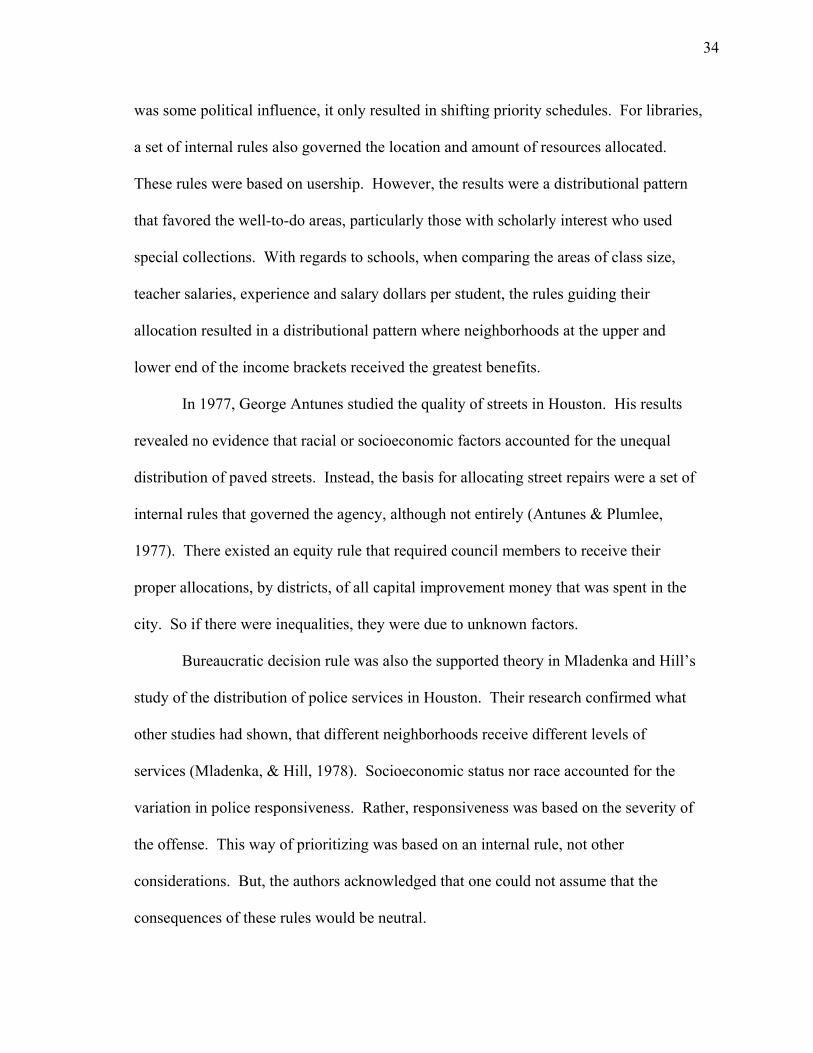
In 1977, George Antunes studied the quality of streets in Houston. His results

revealed no evidence that racial or socioeconomic factors accounted for the unequal

distribution of paved streets. Instead, the basis for allocating street repairs were a set of

internal rules that governed the agency, although not entirely (Antunes & Plumlee,

1977). There existed an equity rule that required council members to receive their

proper allocations, by districts, of all capital improvement money that was spent in the

city. So if there were inequalities, they were due to unknown factors.

Bureaucratic decision rule was also the supported theory in Mladenka and Hill’s

study of the distribution of police services in Houston. Their research confirmed what

other studies had shown, that different neighborhoods receive different levels of

services (Mladenka, & Hill, 1978). Socioeconomic status nor race accounted for the

variation in police responsiveness. Rather, responsiveness was based on the severity of

the offense. This way of prioritizing was based on an internal rule, not other

considerations. But, the authors acknowledged that one could not assume that the

consequences of these rules would be neutral.

35

Kenneth Mladenka, in 1978, decided to reexamine the role of organizational

rules in decision making and their impact on the distribution of urban public services;

namely parks and libraries (Mladenka, 1978). This study included six cities in Virginia

and information was aggregated at the census tract level. Mladenka discovered that

there were no clear cumulative inequalities in either service. Instead, there existed a set

of operational rules that had distributional consequences. These rules, merely simplified

the choice among alternative solutions, reduced uncertainty, made for easy application

and reliable performance, limited discretion and relied on existing agency records and

information. He noted that the reason he focused on the impacts of services rather than

facilities was because he recognized that neighborhoods change easier than physical

facilities. Therefore, the current neighborhood may not resemble the neighborhood that

existed when these services were built.

Bryan Jones and colleagues attempted to show that the distribution of services

had political consequences even though the internal decision making process was

governed by a set of agency rules. Their study of three agencies in the City of Detroit

revealed that the decision rules that were followed did have distributional or political

consequences. However, the nature of the impact and the characteristics of the resulting

distributional patterns varied from agency to agency. They concluded that to better

understand the distributional patterns of a given agency, one should study the internal

structures and processes of that agency (Jones et al., 1978).

Boston was the site of Pietro Nivola’s (1978) study of housing inspection

services. He was concerned that the conventional views of service distribution i.e.

underclass and politics needed to be reconsidered. He concluded that the distributional

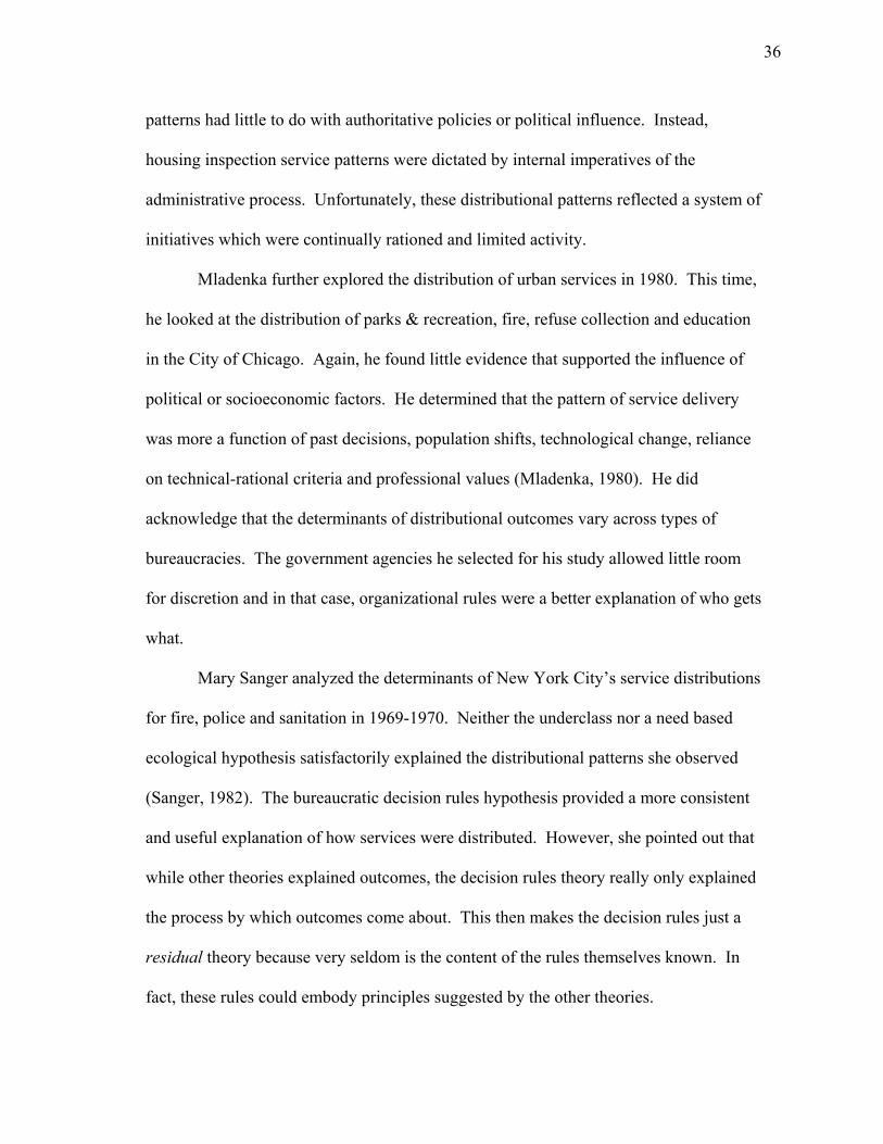
36

patterns had little to do with authoritative policies or political influence. Instead,

housing inspection service patterns were dictated by internal imperatives of the

administrative process. Unfortunately, these distributional patterns reflected a system of

initiatives which were continually rationed and limited activity.

Mladenka further explored the distribution of urban services in 1980. This time,

he looked at the distribution of parks & recreation, fire, refuse collection and education

in the City of Chicago. Again, he found little evidence that supported the influence of

political or socioeconomic factors. He determined that the pattern of service delivery

was more a function of past decisions, population shifts, technological change, reliance

on technical-rational criteria and professional values (Mladenka, 1980). He did

acknowledge that the determinants of distributional outcomes vary across types of

bureaucracies. The government agencies he selected for his study allowed little room

for discretion and in that case, organizational rules were a better explanation of who gets

what.

Mary Sanger analyzed the determinants of New York City’s service distributions

for fire, police and sanitation in 1969-1970. Neither the underclass nor a need based

ecological hypothesis satisfactorily explained the distributional patterns she observed

(Sanger, 1982). The bureaucratic decision rules hypothesis provided a more consistent

and useful explanation of how services were distributed. However, she pointed out that

while other theories explained outcomes, the decision rules theory really only explained

the process by which outcomes come about. This then makes the decision rules just a

residual theory because very seldom is the content of the rules themselves known. In

fact, these rules could embody principles suggested by the other theories.

37

Table 2.3 summarizes the literature supporting the Decision Rules theory of

urban service delivery.

TABLE 2.3: Summary of Decision Rules Literature Author Services Studied Location Measures to Consider

Levy, Meltsner & Wildavsky (1974)

Schools Libraries Streets

Oakland, CA Internal rules Public usage Professional criteria

Antunes & Plumlee (1977)

Streets Houston, TX Internal rules and equity among council districts

Mladenka & Hill (1978)

Police Houston, TX Severity of offense

Mladenka (1978) Parks and libraries 6 cities in Virginia Operational rules Jones et al. (1978) Three agencies Detroit, MI Study the internal process

and structure of agency Nivola (1978) Housing inspection

services Boston, MA Internal imperatives of the

administrative process Mladenka (1980) Parks and recreation

Fire, refuse collection, education

Chicago, IL Past decisions Population shifts Technological changes Technical-rational criteria Professional values

Sanger (1982) Fire Police Sanitation

New York Knowledge of the agencies internal rules

Political Influence

The Political Influence theory supports the contention that the distribution of

services reflects the electoral considerations of politicians (Lee, 1994). These

considerations are influenced by external forces that can include civic pressures or re-

election issues (Meier, Stewart & England, 1991).

Bryan Jones analyzed the role of intermediary groups in delivery of urban public

services. For his study, Jones chose to focus on Chicago’s Department of Buildings.

His objective was to determine whether citizens were linked in any way to the service

bureaucracy through mediating structures and whether these linkages affected the

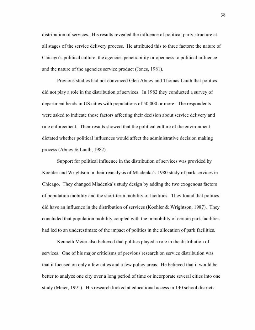
38

distribution of services. His results revealed the influence of political party structure at

all stages of the service delivery process. He attributed this to three factors: the nature of

Chicago’s political culture, the agencies penetrability or openness to political influence

and the nature of the agencies service product (Jones, 1981).

Previous studies had not convinced Glen Abney and Thomas Lauth that politics

did not play a role in the distribution of services. In 1982 they conducted a survey of

department heads in US cities with populations of 50,000 or more. The respondents

were asked to indicate those factors affecting their decision about service delivery and

rule enforcement. Their results showed that the political culture of the environment

dictated whether political influences would affect the administrative decision making

process (Abney & Lauth, 1982).

Support for political influence in the distribution of services was provided by

Koehler and Wrightson in their reanalysis of Mladenka’s 1980 study of park services in

Chicago. They changed Mladenka’s study design by adding the two exogenous factors

of population mobility and the short-term mobility of facilities. They found that politics

did have an influence in the distribution of services (Koehler & Wrightson, 1987). They

concluded that population mobility coupled with the immobility of certain park facilities

had led to an underestimate of the impact of politics in the allocation of park facilities.

Kenneth Meier also believed that politics played a role in the distribution of

services. One of his major criticisms of previous research on service distribution was

that it focused on only a few cities and a few policy areas. He believed that it would be

better to analyze one city over a long period of time or incorporate several cities into one

study (Meier, 1991). His research looked at educational access in 140 school districts

39

across the US. He chose education because he believed it would be most likely

controlled by bureaucratic decision rules and least by electoral politics. He found that

bureaucratic decision rules did not over ride the impact of political forces or social class

biases. In cases where bureaucratic decision rules had been established, thus preventing

bureaucrats from adjusting services to meet either political or social ends, decision rules

determined policy. However, where there was room for discretion, political forces

clearly an exerted influence.

The objective of Rowan and Tunyavong’s study was to reexamine the role of

distributional politics (Rowan & Tunyavong, 1994). In the City of Chicago, they

analyzed the distribution of Community Development Block Grant funds (CDBG) over a

15-year period and Capital Improvement Projects (CIP) over a 6-year period. Their

findings were in support of political influences in service distribution. They concluded

that who rules really does matter. The use of a particular program for political purposes

can occur over short periods of time. Elected officials can be selective by choosing

certain programs for political purposes. Only when it is not to their benefit to do so they

allow bureaucratic decision rules to reign.

Table 2.4 is a summary of the political influence literature.

Additional Studies

In addition to the studies just discussed, there are a number of studies that

propose alternative theories or address service distribution issues.

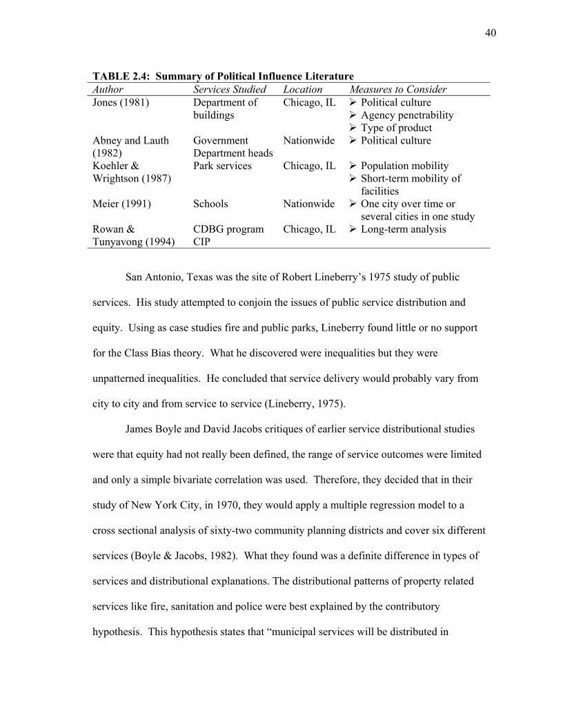
40

TABLE 2.4: Summary of Political Influence Literature Author Services Studied Location Measures to Consider Jones (1981) Department of

buildings Chicago, IL Political culture

Agency penetrability Type of product

Abney and Lauth (1982)

Government Department heads

Nationwide Political culture

Koehler & Wrightson (1987)

Park services Chicago, IL Population mobility Short-term mobility of facilities

Meier (1991) Schools Nationwide One city over time or several cities in one study

Rowan & Tunyavong (1994)

CDBG program CIP

Chicago, IL Long-term analysis

San Antonio, Texas was the site of Robert Lineberry’s 1975 study of public

services. His study attempted to conjoin the issues of public service distribution and

equity. Using as case studies fire and public parks, Lineberry found little or no support

for the Class Bias theory. What he discovered were inequalities but they were

unpatterned inequalities. He concluded that service delivery would probably vary from

city to city and from service to service (Lineberry, 1975).

James Boyle and David Jacobs critiques of earlier service distributional studies

were that equity had not really been defined, the range of service outcomes were limited

and only a simple bivariate correlation was used. Therefore, they decided that in their

study of New York City, in 1970, they would apply a multiple regression model to a

cross sectional analysis of sixty-two community planning districts and cover six different

services (Boyle & Jacobs, 1982). What they found was a definite difference in types of

services and distributional explanations. The distributional patterns of property related

services like fire, sanitation and police were best explained by the contributory

hypothesis. This hypothesis states that “municipal services will be distributed in

41

proportion to tax contributions.” Distribution patterns for social services like health,

welfare and education services were best explained by the compensatory hypothesis.

This states that “municipal services are distributed on the basis of need.” Boyle and

Jacobs further commented that those studies that found no clear distributional pattern

and attributed this to decision rules possibly overlooked or omitted important

explanatory or external variables. They stated that it is not realistic to believe that there

are no external influences in service distribution.

The purpose of Peter Nardulli and Jeffery Stonecash’s research was to provide

the theoretical framework for posing or evaluating any theory of service distribution

(Nardulli & Stonecash, 1982). They believed that previous research had neglected very

important logical questions about possible influences upon distribution. Therefore, they

posed a series of five questions they believed must be considered if a general theory or

an expectation for a specific city is to be formed. The questions, in suggested order, are

as follows:

1. What is the nature of services (can the service be unequally distributed)?

2. What is the nature of the bureaucracy (it is susceptible to political influence

and/or does a bureaucratic policy exist.)

3. What are the rules of allocation the organization uses?

4. If the bureaucracy is susceptible to external influences, whit kind of political

linkages exits?

5. What are the distributional patterns desired by the bureaucracy?

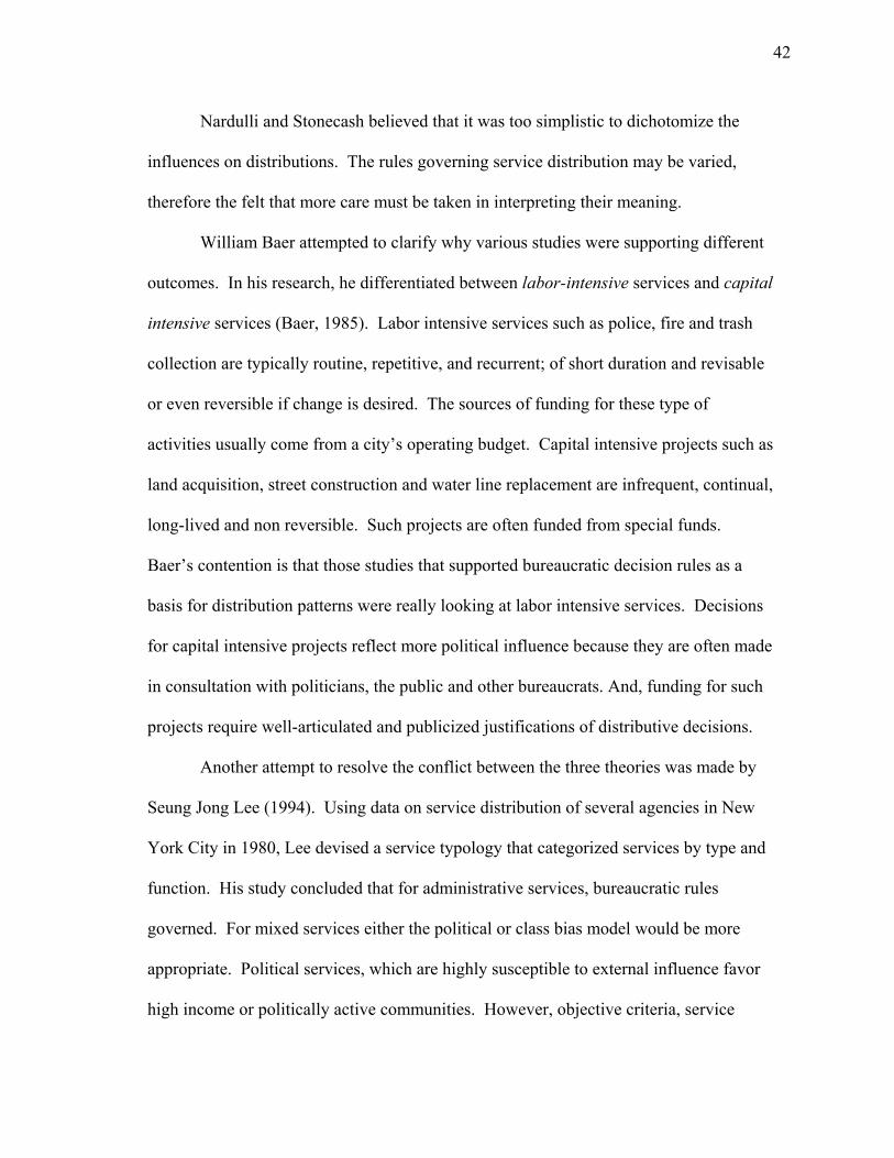
42

Nardulli and Stonecash believed that it was too simplistic to dichotomize the

influences on distributions. The rules governing service distribution may be varied,

therefore the felt that more care must be taken in interpreting their meaning.

William Baer attempted to clarify why various studies were supporting different

outcomes. In his research, he differentiated between labor-intensive services and capital

intensive services (Baer, 1985). Labor intensive services such as police, fire and trash

collection are typically routine, repetitive, and recurrent; of short duration and revisable

or even reversible if change is desired. The sources of funding for these type of

activities usually come from a city’s operating budget. Capital intensive projects such as

land acquisition, street construction and water line replacement are infrequent, continual,

long-lived and non reversible. Such projects are often funded from special funds.

Baer’s contention is that those studies that supported bureaucratic decision rules as a

basis for distribution patterns were really looking at labor intensive services. Decisions

for capital intensive projects reflect more political influence because they are often made

in consultation with politicians, the public and other bureaucrats. And, funding for such

projects require well-articulated and publicized justifications of distributive decisions.

Another attempt to resolve the conflict between the three theories was made by

Seung Jong Lee (1994). Using data on service distribution of several agencies in New

York City in 1980, Lee devised a service typology that categorized services by type and

function. His study concluded that for administrative services, bureaucratic rules

governed. For mixed services either the political or class bias model would be more

appropriate. Political services, which are highly susceptible to external influence favor

high income or politically active communities. However, objective criteria, service

43

needs and conditions proved to be more important determinates of service distribution,

regardless of the service type.

Table 2.5 summarizes the findings of the additional studies.

TABLE 2.5: Summary of Additional Studies Author Services

Studied Location Findings

Lineberry (1975) Parks Fire

San Antonio, TX Unpatterned inequalities that vary from city to city and from service to service

Boyle & Jacobs (1982)

Variety New York City Different in types of services and distributional patterns; patterns depending on nature of service

Nardulli & Stonecash (1982)

Not dichotomize the influences or distributions

Baer (1985) Variety Type of services: capital intensive vs. labor intensive, dictated type influence

Lee (1994) Variety New York City Service type, objective criteria service needs and conditions dictate influence

Contributions of Current Research

A majority of the research on citizen contacts identifies who makes contact, why

they make contact and the bureaucracy’s immediate response. The effects of citizen

initiated contacts, on public policy have received little attention (Rosener, 1978; Potter

& Norville, 1983; Thomas & Melkers, 1999). This study intends to extend what is

known about government’s response to citizen initiated contacts by determining if these

contacts effect long-range policy.

44

This research will also contribute to the body of knowledge on service

distribution. Though there a number of studies on service distribution patterns, their

research suggest gaps that should be address. Those gaps which are addressed in this

study include: reviewing the internal structure and process of the agency as part of

evaluating the distribution of services (Jones et al., 1978); taking a closer look at the

rules embodied within the agency (Sanger, 1982); studying the same city and services

over time in order to detect changes in distributional patterns and the use of multiple

indicators (Mladenka, 1989).

In addition to research on service distribution, this study attempts to understand

the decision making process with regards to infrastructure repair/replacement allocation

and the Public Works Department. It is accepted that infrastructure decision making

models can no longer be solely a technical issue (Rittel & Webber, 1973). However, it is

unclear how non-technical issues are being incorporated into the current decision making

process. This research will determine if and how non-technical issues are being

integrated into the infrastructure policy-making process.

45

CHAPTER III

METHODOLOGY

In Houston, the repair and maintenance of water and sewer elements are

managed by different branches within the Public Utilities Division. However, Capital

Improvement Projects for both infrastructure elements are funded from the same source

and follow virtually the same decision making process. For those reasons, both are part

of this study.

This chapter will state the research and null hypotheses, outline the study design,

define the variables and explain the statistical procedures to be used.

Research Hypotheses

To achieve the objectives of determining the statistical significance of citizen

contacts on the selection of water and sewer capital improvement projects, this study

will test five null hypotheses. Each of the null hypotheses tests the significance of

citizen contacts on the selection of water and sewer capital improvement projects

singularly and in the presence of other variables.

Direct Relationship Between Work Orders and Project Selection

Hypothesis 1a. Citizen initiated contacts have had a significant effect on the selection of

water related capital improvement projects between 1992 and 1999.

46

Null Hypothesis 1a. Citizen initiated contacts have had no significant effect on the

selection of water related capital improvement projects between 1992 and 1999.

Hypothesis 1b. Citizen initiated contacts have had a significant effect on the selection of

sewer related capital improvement projects between 1992 and 1999.

Null Hypothesis 1b. Citizen initiated contacts have had no significant effect on the

selection of sewer related capital improvement projects between 1992 and 1999.

Hypotheses Representing the Class Bias Theory

Hypothesis 2a. Citizen initiated contacts, when taken in consideration with

sociodemographic variables, have had a significant effect on the selection of

water related capital improvement projects between 1992 and 1999.

Null Hypothesis 2a. Citizen initiated contacts, when taken in consideration with

sociodemographic variables, have had no significant effect on the selection of

water related capital improvement projects between 1992 and 1999.

Hypothesis 2b. Citizen initiated contacts, when taken in consideration with

sociodemographic variables, have had a significant effect on the selection of

sewer related capital improvement projects between 1992 and 1999.

Null Hypothesis 2b. Citizen initiated contacts, when taken in consideration with

sociodemographic variables, have had no significant effect on the selection of

sewer related capital improvement projects between 1992 and 1999.

47

Hypotheses Representing Decision Rule Theory

Hypothesis 3a. Citizen initiated contacts, when taken in consideration with technical

factors, have had a significant effect on the selection of water related capital

improvement projects between 1992 and 1999.

Null Hypothesis 3a. Citizen initiated contacts, when taken in consideration with

technical factors, have had no significant effect on the selection of water related

capital improvement projects between 1992 and 1999.

Hypothesis 3b. Citizen initiated contacts, when taken in consideration with technical

factors, have had a significant effect on the selection of sewer related capital

improvement projects between 1992 and 1999.

Null Hypothesis 3b. Citizen initiated contacts, when taken in consideration with

technical factors, have had no significant effect on the selection of sewer related

capital improvement projects between 1992 and 1999.

Hypotheses Representing Political Theory

Hypothesis 4a. Citizen initiated contacts, when taken in consideration with political

factors, have had a significant effect on the selection of water related capital

improvement projects between 1992 and 1999.

Null Hypothesis 4a. Citizen initiated contacts, when taken in consideration with

political factors, have had no significant effect on the selection of water related

capital improvement projects between 1992 and 1999.

48

Hypothesis 4b. Citizen initiated contacts, when taken in consideration with political

factors, have had a significant effect on the selection of sewer related capital

improvement projects between 1992 and 1999.

Null Hypothesis 4b. Citizen initiated contacts, when taken in consideration with

political factors, have had no significant effect on the selection of sewer related

capital improvement projects between 1992 and 1999.

Hypotheses Incorporating All Variables

Hypothesis 5a. Citizen initiated contacts, when taken in consideration with all other

factors, have had a significant effect on the selection of water related capital

improvement projects between 1992 and 1999.

Null Hypothesis 5a. Citizen initiated contacts, when taken in consideration with all

other factors, have had no significant effect on the selection of water related

capital improvement projects between 1992 and 1999.

Hypothesis 5b. Citizen initiated contacts, when taken in consideration with all other

factors, have had a significant effect on the selection of sewer related capital

improvement projects between 1992 and 1999.

Null Hypothesis 5b. Citizen initiated contacts, when taken in consideration with all

other factors, have had no significant effect on the selection of sewer related

capital improvement projects between 1992 and 1999.

49

Research Design

This research is a quantitatively analyzed case study designed with the purpose

of describing and diagnosing the factors considered in the selection of sewer and water

projects for Houston’s Capital Improvement Plan. The study is longitudinal in nature;

covering the time period beginning in 1992 (the year the city's maintenance system

became computerized) through 1999. A longitudinal study was chosen because it will

allow for technological, administrative and political changes that may occur over time.

The target population is the City of Houston, Texas. Houston was chosen for

two reasons. First, when the research began, the Department of Public Works and

Engineering was in the process of upgrading their GIS and Infrastructure Management

System. Secondly, the city was working with Texas A&M University on an

infrastructure project funded by the National Science Foundation. This research is an

extension of that project.

The city has various levels of analysis that could be studied: census tracts, zip

codes, Key Maps, Inc., neighborhood, super neighborhoods and voting districts. Census

tracts were chosen for this research because of the availability of demographic data; the

existence of concrete, non-subjective boundaries; and the constancy of the boundaries

during the study period.

Of the 481 census tracts in Houston, only those tracts that had at least one-third

of its land mass within the city’s boundaries were considered. Seven tracts were omitted

from the study because they were commercial areas (downtown and the Galleria) that

50

have ongoing projects and thus are not subjected the same annual CIP selection process.

In total, 375 census tracts were studied.

Dependent Variables

Two dependent variables will be measured. Water related projects (WCIP) and

sewer related projects (SCIP) are capital improvement projects approved by City

Council 1992-1999. The dependent variable will only include work on underground

lines and valves. Treatment plants, towers, lift and pump stations, etc. will not be

studied because they are visible features of the water system and this study focuses on

underground, non-visible elements. Also, towers and treatment plants have little if no

interaction with the public. Citizen complaints address local problems, not global

problems. Major rehabilitation or replacement projects are driven by capacity or

regulatory issues although these issues can cause local problems.

The dependent variable will be dichotomous in nature, taking on the values of

either (0) no project allocated that year or (1) project(s) allocated that year.

Independent Variables

Citizen initiated contacts may not be the only factor that contributes to the

selection of water and sewer replacement projects. Therefore, this study includes other

variables that may be considered by the Department of Public Works and those who

affect the selection of CIP projects. The independent variables have been identified in

51

the literature and via formal and informal interviews with PW&E staff and City Council

members.

Citizen calls will be represented by work orders. During the study period, all

citizen complaints or requests for utilities determined to be the city’s

responsibility, resulted in either water work orders (WWO) or sewer work

orders (SWO). Between 1992 and 1995, PW&E began gathering and

summarizing data in the spring prior to June 30th (end of fiscal year). In

1996, their planning process began earlier and data was summarized the

previous winter. Therefore, the number of calls will be calculated March to

February for years 1992 through 1995 and on a calendar year 1997 through

1999. Year 1996 will capture work orders beginning March 1995 through

December 1995.

Variables Representing the Class Bias Theory

Racial composition is the percent non-white population as of the 1990 census

(NONWHITE). This percent is calculated as the number of non-white

persons divided by the total population.

Median household income according to the 1990 census (INC).

Percent home owner in 1990 (OWN). This number is calculated as the

number of owner-occupied housing divided by the number of occupied

housing units.

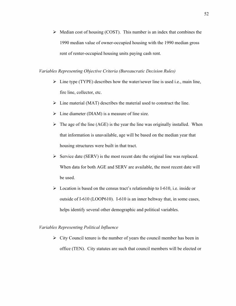
52

Median cost of housing (COST). This number is an index that combines the

1990 median value of owner-occupied housing with the 1990 median gross

rent of renter-occupied housing units paying cash rent.

Variables Representing Objective Criteria (Bureaucratic Decision Rules)

Line type (TYPE) describes how the water/sewer line is used i.e., main line,

fire line, collector, etc.

Line material (MAT) describes the material used to construct the line.

Line diameter (DIAM) is a measure of line size.

The age of the line (AGE) is the year the line was originally installed. When

that information is unavailable, age will be based on the median year that

housing structures were built in that tract.

Service date (SERV) is the most recent date the original line was replaced.

When data for both AGE and SERV are available, the most recent date will

be used.

Location is based on the census tract’s relationship to I-610, i.e. inside or

outside of I-610 (LOOP610). I-610 is an inner beltway that, in some cases,

helps identify several other demographic and political variables.

Variables Representing Political Influence

City Council tenure is the number of years the council member has been in

office (TEN). City statutes are such that council members will be elected or

53

re-elected for a two-year term. The maximum number of terms that can be

served is three.

Electoral influence is described by the variable percent registered to vote

(VOTE). It is the number of registered voters divided by census tract

population.

Stable (STABLE) indicates if a precinct has been redistricted during the

study period

Percent of the population that is active (ACTIVE) is the number of citizen

calls divided by census tract population.

Districts (DIST) represent the nine council districts in Houston.

Data Sources

The data used is archival, originally collected by various city departments and

organizations. This section describes the characteristics of each database provided by

source.

The Planning and Development Department provides an Arcview database,

COHGIS, release five. COHGIS contains a variety of layers that will be used

in this study. These layers include: city limits, council districts, counties,

neighborhood to standard areas, super neighborhoods and capital

improvement projects. The strength of this database is the amount of

information that it contains and the fact that it is in tabular and graphical

formats. The weakness is that the layers are updated at different times.

54

Therefore, before comparisons are made, it is necessary to update the older

layers to correspond with the most recent.

Harris County Tax Assessor's office offers a computerized precinct map and

a list of all registered voters by precinct, by year. A weakness of the voter

database is that it may be current but not necessarily accurate.

The Department of Public Works and Engineering maintains

1. A GIMS database that describes water and sewer lines. A weakness of

this database is that not all the fields have information. The method for

collecting, entering and updating information is unclear. Therefore, one

does not know how recent the information is. A second weakness is that

historical information is lost when a line segment is replaced. The

strength of the database lies in that it provides relatively accurate location

and description of water and sewer lines.

2. An IMS database that contains citizen contact and work order records for

1992 through June, 1999. The strength of the database is that it is fairly

complete, provides location of call, date and time; it also tracks work

orders until work is completed. Most importantly, it ties service requests

to work orders so that service request and work order numbers can be

coordinated. The weakness of IMS stems from changes in record keeping

throughout the study period. Work orders were initially maintained by

separate offices with jurisdiction over city quadrants and were transferred

to a central location in the mid 1990’s. There may be a possible loss of

55

records and changes in the way data was recorded. Also, the level of

completeness varies from work order record to record.

3. The CIP documents which describe the individual projects. The

weakness of this source is that there are instances where the approved

CIP project is substituted by another. This may happen at the design

phase and therefore would not be included within the document nor

would the substitution show in subsequent years.

The Bureau of the Census has 1990 demographic information on the census

tracts that are part of the city of Houston. The demographics selected contain

racial composition, median household income, percent homeownership,

average cost of housing and median housing age. The strength of this

database is that its numbers and percentages are commonly recognized and

used.

The Houston Chronicle newspaper supplied political information relating to

council districts, tenure, election years and redistricting. All archived

editions are accessed on-line.

In addition to the data collected, formal and informal interviews were held with

persons from the various divisions within the Department of Public Works and

Engineering and select council members. The purpose of the interviews were to have a

better understanding of how the data was used and to identify the players in the decision

making process. When permitted, interviews were tape recorded for accuracy.

56

Data Analysis

Three levels of analysis were performed: descriptive univariate analysis,

comparative bivariate analysis, and explanatory multivariate analysis.

Descriptive Univariate Analysis

A univariate analysis is useful for three reasons (Hatcher & Stepanski, 1994). It

screens the data, helping to identify data keyed in incorrectly and to ensure that data can

be read and manipulated by the computer. Secondly, it reveals the shape of the data.

This will help to determine if the data is normally distributed or if transformations need

to be made. Finally, the analysis will provide a basic description of the data i.e.

minimum, maximum, mean, frequency and measures of central tendency.

Bivariate Analysis of Variable Relationships

A bivariate analysis was used to determine the strength and direction of the

relationships among the independent variables and between the dependent and

independent variables (Healey, 1984). Because the variables are measured differently,

several measures were used. The chi-square test of independence was used to test the

relationship between two categorical variables. While the chi-square test statistic tests

the significance of the relationship, there are two chi-square based statistics that assess

the strength of the relationship. The Phi θ coefficient is used for 2 x 2 tables, the

Cramer’s V statistic is applied to larger tables (Healey, 1984). Where appropriate, either

of these statistics will be calculated. Pearson’s rho measured the relationship between

integer variables. Kendall’s Tau-b was used for measuring the association between two

57

ordinal variables and between ordinal and integer variables. A t-test measured the

relationship between categorical and integer variables and a Kruskal-Wallis test was

used on ordinal and categorical variables.

Multivariate Analysis

A multivariate logistic regression analysis was used to determine the importance

of the independent variables on the selection of CIP projects. Logistic regression was

chosen because it is specifically designed for modeling the relationship between a

discrete, dichotomous dependent variable and one or more independent variables

(Hosemer & Lemeshow, 2000).

For both water and sewer, five separate logistic regression models were run. As

shown in the example below, the first model tests for a direct relationship between work

orders and the dependent variable.

Simple model: ((x) (water project allocation) =

e B(0) + B(1) x(1) 1 + e B(0) + B(1) x(1)

where x(1) = WWO or SWO

Three of the five models are theory based and will test the individual and

interactive effects of the independent variables on CIP project selection and the fit of the

model in predicting the dependent variable, CIP. The example below is the logistic

regression for the Class Bias Model.

58

Class Bias Model: ((x) (water project allocation) =

e B(0) + B(1)x(1) + B(2) x(2) + B(3) x(3) + B(4)x(4) + B(5) x(5) 1 + e B(0) + B(1)x(1) + B(2) x(2) + B(3) x(3) + B(4)x(4) + B(5) x(5)

where x1 = WWO or SWO x2 = NONWHITE

x3 = INC x4 = OWN x5 = COST The fifth model is a full model examining the contribution of all the independent

variables on the dependent variable irrespective of theoretical considerations.

Full Model: ((x) (water project allocation) =

e B(0) + B(1)x(1) + B(2) x(2) + B(3) x(3) + B(4)x(4) + B(5) x(5) +B(6)x(6) + B(7)x(7) + … B( )x( ) 1 + e B(0) + B(1)x(1) + B(2) x(2) + B(3) x(3) + B(4)x(4) + B(5) x(5)+B(6)x(6) + B(7)x(7) + … B( )x( )

Two statistics were used to determine the independent variable(s) relationship

with the dependent variable. The first is the Wald chi-Square statistic. This statistic

functions like the chi-square in a Least Squares regression. The significance level is set

for .05. The second, and more reliable statistic, is the Odds Ratio and related 95 percent

confidence interval. The Odds Ratio describes the magnitude of the relationship

(Dawson-Saunders & Trapp, 1990). It expresses the likelihood of an occurrence i.e.

census tract receiving a CIP project, relative to the likelihood of a non-occurrence. The

ratio ranges from negative infinity to positive infinity. The stronger the relationship

between the independent and dependent variable is in the distance the ratio is from

1.000. A value of 1.000 indicates no relationship.

59

To assess model fit, the -2 Log Likelihood, Likelihood Ratio and Score statistics

were used. Lower values of the 2-Log Likelihood statistic indicate a more desirable

model. The Likelihood Ratio and Score statistics have a chi-square distribution with a p-

value for the statistic.

60

CHAPTER IV

THEORETICAL MODEL ANALYSIS

Introduction

The three theories of urban service delivery provide the framework used to

analyze the data. By the single variable work order and then by theory, this chapter will

first provide a univariate analysis of the variables. The analysis will briefly describe the

data and discuss what, if any, transformations were needed to present the data in a

manageable, quantitative form without losing too much of the information provided in

the raw data. Next, the bivariate relationships will be examined between work orders

and the theory based independent variables, among the theory-based variables and

between the independent and dependent variables. Finally, the results of the multivariate

analysis will be discussed.

Simple Model

Univariate analysis

A total of 330,046 water related and 253,226 sewer related citizen calls were

logged in the selected census tracts during the eight-year study period. Though there

were fluctuations throughout the years, the volume of calls have been increased from

approximately 17,000 water and 10,800 sewer in 1992 to 56,316 water and 38,343 sewer

61

calls in 1999. These calls represent an average of, respectively, 150 and 105 calls per

calendar day.

Figure 4.1 summarizes the annual work orders for both water and sewer.

Between the second and third years, the number of water work orders almost doubled.

After 1994, the number of calls began to decrease until 1997. After a 23 percent

decrease in water related calls in 1998, the number of calls reached its maximum of

56,316 in 1999.

The number of sewer work orders increased by 60 percent between 1992 and

1993 and by 80 percent between 1993 and 1994. After 1995, the number of calls

dropped from 34,308 to 29, 434. The number of calls increased the following year and

reached its peak of 38,343 in 1999.

Figure 4.1: Water and Sewer Related Complaints

0

10,000

20,000

30,000

40,000

50,000

60,000

92 93 94 95 96 97 98 99

Water Sewer

62

Water and sewer work orders were aggregated by census tracts. The description

data is presented in Table 4.1. When aggregated, work orders were not normally

distributed nor did they meet the condition of independence from year to year. Calls are

carried over to the next year if no corresponding capital improvement project had been

allocated. Therefore, to facilitate further analysis, both water and sewer work orders

were divided into quartiles based on the median. A description of all the independent

variables after the transformations are in Appendix A.

TABLE 4.1: Number of Water and Sewer Work Orders by Census Tract Variable Min Max Mean Median Std. Dev

Water WWO92 0 163 45.24 33.014 38.00 WWO93 0 396 97.53 64.33 89.00 WWO94 0 859 218.63 138.61 192.00 WWO95 0 1316 310.30 212.82 280.00 WWO96 0 1786 369.229 260.267 315.00 WWO97 2.0 2420 472.610 330.24 404.00 WWO98 7. 2897 499.730 396.24 417.00 WWO99 11.0 2608 593.674 430.288 491.00 Sewer SWO92 0 203 28.74 29.54 20.00 SWO93 0 551 70.22 68.51 52.00 SWO94 0 1007 147.62 136.63 107.00 SWO95 0 1499 225.07 200.64 165.00 SWO96 0 1919 284.46 216.0 257.65 SWO97 0 2377 358.79 277.0 330.15 SWO98 0 2811 396.58 287.0 298.00 SWO99 0 3278 467.49 334.0 469.56

63

Multivariate Analysis

The results of the regression model are presented in Table 4.2. The p-values of

the multivariate analysis indicate that for five years during the eight-year period (1992,

1993, 1997, 1998 and 1999) water work orders significantly predicted the likelihood that

a capital improvement project would be selected in a given census tract. The Odds Ratio

indicates that the strongest relationships between water work orders and capital

improvement projects are in 1992. In that year, the odds that a census tract with a work

order received a capital improvement project is 2.026, or twice as likely than for a

census tract without a work order. The corresponding confidence interval contains the

value of the true ratio. Since the interval does not contain 1.000 (an indication of no

relationship) we can be 95 percent confident that the relationship is indeed significant.

After 1992, the ability of work orders to predict a water capital improvement project

decreases. In 1993, there is only a 47 percent likelihood that a census tract with a work

order was allocated a capital improvement project versus one with no work orders. In

1997, there was a 38 percent likelihood. The likelihood increases in 1998 to 55 percent

and increases again in 1999 to 70 percent. In none of these years do the corresponding

confidence intervals encompass 1.000. Therefore, we are 95 percent confident of the

strength of those relationships. Since water work orders has had a significant influence

on the prediction of capital improvement projects 62 percent of the time, we can reject

the null hypothesis 1a.

64

TABLE 4.2: Effects of Citizen Contact on CIP Projects (n=375) Year Estimate (p-value) Odds Ratio Confidence Interval

Water WWO92 .7060 .0001* 2.026 (1554, 2.641) WWO93 .3872 .0275* 1.473 (1.044, 2.078) WWO94 .1066 .4591 1.112 (.839, 1.475) WWO95 .2045 .1244 1.227 (.945, 1.592) WWO96 .2273 .1735 1.255 (.905, 1.741) WWO97 .3237 .0159* 1.382 (1.063, 1.798) WWO98 .4434 .0121* 1.558 (1.102, 2.203) WWO99 .5359 .0069* 1.709 (1.159, 2.521) Sewer SWO92 .2166 .1079 1.242 (.954, 1.617) SWO93 .0651 .6661 1.067 (.794, 1.435) SWO94 .4609 .0269* 1.585 (1.054, 2.384) SWO95 .1605 .3615 1.174 (.832, 1.657) SWO96 .0785 .6565 1.079 (.772, 1.507) SWO97 .4201 .0025* 1.522 (1.159, 2.000) SWO98 .2745 .1259 1.316 (.926, 1.870) SWO99 .5268 .0078* 1.649 (1.148, 2.497) *Significant at the .05 level

Sewer work orders significantly predict the likelihood of selecting a capital

improvement projects in years 1994, 1997 and 1999. Unlike water, the strength or

magnitude of the significant relationships of sewer work orders with the dependent

variable were relatively consistent. As reflected in the Odds Ratios, census tracts with

work orders had a 58 percent likelihood of receiving a capital improvement project, in

1994, versus those tracts with no work orders. In 1997 there was a 52 percent chance

and in 1999 a 64 percent chance of a census tract receiving a capital improvement

project if there had been a work order. The number of years where work orders had a

significant effect on project allocation, was a low 37 percent (3/8) of the time. Still we

can reject null hypothesis 1b for sewer work orders has proven to be a significant

predictor for three of the study years.

65

Model Fit

A review of the water model fit shown in Table 4.3 reveals that when compared

with the intercept only, the model where water work orders is statistically significant is a

better fit 37 percent of the time. The values of the –2 Log Likelihood are shown with the

intercept only and with the inclusion of the covariates. A decrease in value signifies a

model improvement. The Likelihood Ratio chi-square measures the difference between

the two. According to that value, there is a model improvement by adding water work

orders. The improvement ranges from .55 in 1994 to 31.71 in 1992. But, is the

improvement significant? The p-values associated with the Likelihood Ratio and the

Score value indicate that the model improvement is significant in every year except

1994, 1995 and 1996. These coincide with the years where no significant variables were

identified.

The inclusion of sewer work orders has also been a model improvement for every

year. In 1993, the improvement was a low .18. In 1999, the model improvement was by

8 points. However, the model improvement was significant for only the three years,

1994, 1997 and 1998 where there were significant variables. This conclusion is

supported by the chi-square significance of the Likelihood Ratio and Score values.

The results of the multivariate analysis indicate that work orders do not account

for all CIP projects. Fortunately, this is not where the analysis ends. The next step is to

incorporate the previously discussed models to determine potential group and individual

effects.

66

TABLE 4.3: Simple Model Fit Comparisons (n=375) -2 Log Likelihood Likelihood Ratio Score Value

Intercept Only

With covariates chi-square p-value chi-square p-value

Water 1992 363.941 332.224 31.7173 .0001 30.1832 .0001 1993 232.637 227.552 5.0850 .0241 5.0100 .0252 1994 290.739 290.189 .5501 .4583 .5493 .4586 1995 309.119 306.724 2.3955 .1217 2.3848 .1225 1996 218.704 216.811 1.8938 .1688 1.8772 .1707 1997 316.163 310.125 6.0386 .0140 5.9567 .0147 1998 209.077 202.221 6.8556 .0088 6.6573 .0099 1999 194.086 185.930 8.1568 .0043 7.8526 .0051 Sewer 1992 275.194 272.559 2.6348 .1045 2.6202 .1055 1993 232.637 232.451 .1866 .6658 .1864 .6659 1994 172.965 167.600 5.3656 .0205 5.1883 .0227 1995 199.160 198.317 .8430 .3585 .8386 .3598 1996 199.160 198.961 .1984 .6560 .1982 .6562 1997 294.506 284.760 9.7463 .0018 9.5296 .0020 1998 183.698 181.261 2.4366 .1185 2.400 .1213 1999 183.698 175.639 8.0581 .0045 7.6989 .0078 *Significant at the .05 value

Class Bias Theory

Univariate Analysis

The four variables representing the class bias model are: percent nonwhite

(NONWHITE), percent ownership (OWN), median household income (INC) and

median housing cost (COST). As shown in Table 4.4, percent nonwhite ranges in value

from 0 to 100. Slightly less than half (48 percent) of the census tracts are at least 39

percent nonwhite and 30 percent of the census tracts are over 50 percent non-white. The

values for income, range from 0 to 350,131. But, over 90 percent of the census tracts

had average incomes less than $50,000. Since neither of these variables fit a normal

distribution they were divided into categories. Percent nonwhite was divided into

67

quartiles with values based on the median. Income was trichotomized, with the category

values also based on the median. Appendix A describes the class bias variables after the

transformations.

TABLE 4.4: Description of Class Bias Variables (n=375) Variable Min Max Mean Median Std. Dev

NONWHITE 0 100 43.989 39.00 30.093 INC 0 350,131 29,986 25,644 23,619 OWN 0 100 45.0533 46.00 22.9719 COST 5.594 10.50 5.594 5.500 1.7581

The values for percent ownership ranged from 0 to 100 percent. The median

values revealed that almost 50 percent of the population were homeowners. Housing

cost is the combined average of median rent and median housing values. Both median

rent and median housing values were scaled from 1 to 11. The values were then added

together and divided by 2. The result is the variable housing cost (COST) with values

ranging from 0 to 10.5 with a median value of 5.5 resulting in a normal distribution

throughout the census tracts.

Bivariate Relationships

Relationships between work orders and class bias variables. The relationships

between water work orders (WWO) and the independent variables are described in

Table 4.5. Percent nonwhite and water work orders had a significant relationship

between 1994 and 1998 however, that relationship was weak. The nature or direction of

the relationship indicates that the two variables are negatively related; therefore, we can

68

conclude that in every year, larger numbers of work orders are associated with a smaller

percent of nonwhites.

TABLE 4.5: Bivariate Relationship among Class Bias Variables Variable Percent non-white Median income Percent ownership Housing cost

WWO92 B= -.0809 (.0611) B= .0727 (.1113) P= -.0351 (.4970) P= .0876 (.0900) WWO93 B= -.0623 (.1498) B= .0272 (.5511) P= -.0729 (.1586) P= .0730 (.1581) WWO94 B= -.1157 (.0075) B= .0744 (.1038) P= -.0124 (.8102) P= .1098 (.0334) WWO95 B= -.1595 (.0002) B= .1056 (.0209) P= -.0173 (.7384) P= .1393 (.0069) WWO96 B= -.1670 (.0001) B= .0778 (.0891) P= -.0333 (.5202) P= .1521 (.0031) WWO97 B= -.1315 (.0024) B= .0604 (.1863) P= .0033 (.9481) P= .0696 (.1783) WWO98 B= -.0911 (.0351) B= .0306 (.5029) P= -.0148 (.7749) P= .0318 (.5389) WWO99 B= -.0727 (.0927) B= -.0170 (.7098) P= -.0098 (.8496) P= -.0033 (.9484) NONWHITE B= -.6320 (.0001) P= -.2250 (.0001) P= -.6353 (.0001) INC P= .3839 (.0001) P= .7255 (.0001) OWN P= .2528 (.0001) COST WCIP92 L= -.0544 (.6290) L= .3362 (.1415) L= -.0015 (.7925) L= .0858 (.2496) WCIP93 L= .3959 (.0134) L= -.4578 (.1403) L= 0.0013 (.8596) L= -.2570 (.0214) WCIP94 L= .4722 (.0009) L= -.5217 (.0528) L= .0006 (.9181) L= -.2158 (.0299) WCIP95 L= .1204 (.9132) L= -.0318 (.9000) L= .0019 (.7675) L= -.0330 (.6977) WCIP96 L= .1546 (.3309) L-.0640 (.8405) L= -.0060 (.4558) L= .1299 (.2063) WCIP97 L= -.0217 (.8608) L= .0533 (.8309) L= -.0050 (.4231) L= .0253 (.7589) WCIP98 L= -.3203 (.0599) L= 1.258 (.0003) L= .0018 (.8266) L= .3379 (.0013) WCIP99 L= .0237 (.8894) L= .5633 (.1036) L-.0049 (.5684) L= .0317 (.7797) SWO92 B= -.1058 (.0146) B= .0652 (.1550) P= -.0496 (.3373) P= .0791 (.1261) SWO93 B= -.1176 (.0066) B= .0629 (.1689) P= -.0406 (.4328) P= .0566 (.0977) SWO94 B= -.1020 (.0186) B= .3772 (.4105) P= -.0351 (.4976) P= .0819 (.1131) SWO95 B= -.1081 (.0125) B= .0539 (.2395) P= -.0181 (.7257) P= .0611 (.2375) SWO96 B= -.1173 (.0067) B= .0591 (.1961) P= -.0276 (.5934) P= .0812 (.1161) SWO97 B= -.1004 (.0202) B= .0507 (.2674) P= .0132 (.7976) P= .0410 (.4285) SWO98 B= -.0105 (.8187) B= -.0105 (.8187) P= -.0457 (.3771) P= -.0275 (.6001) SWO99 B= -.0392 (.3918) B= -.0392 (.3918) P= -.0196 (.7039) P= -.0836 (.1058) SCIP92 L= -.0855 (.5298) L= .5995 (.0315) L= -.0020 (.7690) L= .2094 (.0180) SCIP93 L= .3959 (.0139) L= -.4578 (.1403) L= -.0013 (.8596) L=-.2570 (.0214) SCIP94 L= .2718 (.1506) L= -.0551 (.1449) L= -.0013 (.8864) L= -.1049 (.4110) SCIP95 L= .2654 (.1234) L= -.3544 (.2996) L= .0019 (.8205) L= -.1272 (.2783) SCIP96 L= .0925 (.5818) L= .1062 (.7535) L= -.0100 (.2478) L= .1564 (.1499) SCIP97 L= .1568 (.2314) L= .3987 (.1305) L= -.0005 (.9332) L= .1492 (.0793) SCIP98 L= -.3271 (.0782) L= 1.092 (.0032) L= -.0018 (.8403) L= .3245 (.0042) SCIP99 L= .0270 (.8784) L= .5617 (.1183) L= .0063 (.4841) L= .0159 (.8931) = Indicates significance at p=<.05 B=Kendall’s Tau-b P=Pearson’s rho L=Logistic regression

69

The relationship between water work orders and income is positively significant

in 1995. Housing cost and water work orders have a positively significant, albeit weak,

relationship between 1994 and 1996.

Percent nonwhite was the only class bias variable to have a significant

relationship with sewer work orders (SWO). This occurred between 1992 and 1997.

The relationship between the two variables is negative and the value of the correlation

coefficient indicates that the relationship is weak.

Associations among class bias variables. All the relationships among the class

bias variables are significant. However, they vary on the strength of the correlation and

the direction of the relationship. A moderately strong negative relationship exists

between percent nonwhite and income and between percent nonwhite and housing cost.

As might be expected, lower incomes and lower housing costs are associated with higher

percentages of non-whites. The correlation between percent nonwhite and percent

ownership is negative and not as strong. The strongest correlation among the class bias

variables is the positive relationship between income and housing cost. The relationship

between percent ownership and housing cost is also positive but not nearly as strong.

Associations between class bias and dependent variables. The relationships

between work orders and the dependent variable were discussed in the first section of

this chapter. The relationship between the class bias and dependent variables, also

shown in Table 4.5, vary from year to year. In 1992, between 1995 and 1997 and 1999,

there were no significant relationships between water capital improvement projects

(WCIP) and any of the class bias variables. In 1993 and 1994, percent nonwhite and

housing cost were significant and the direction of those relationships are positive. In

70

1998, water capital improvement projects had a positive significant relationship with

both income and housing cost.

For sewer, the only significant relationship in 1992 is the positive relationship

between housing cost and sewer capital improvement projects. In 1993, the significant

relationships were the positive relationship with percent nonwhite and the negative

relationship with housing cost. In 1994 through 1997 and again in 1999, there were no

significant relationships. In 1998, sewer capital improvement projects had a positive

significant relationship with both income and housing cost.

Multivariate Analysis

From the results of the bivariate analysis, we can conclude that the variable

percent ownership, because it has no significant relationship with the dependent

variables, could be omitted from further analysis. A series of logistic regressions

confirms this.1 Table 4.6 shows the outcome of regression models run for each year.

For brevity, only significant variables are displayed. A detailed output of all variables

along with the model fit statistics can be found in Appendix B.

Beginning with water, even with the addition of other variables and with little

effect on the strength of the Odds Ratio, water work orders remained positively

significant in the same years as in the simple model.

1Stepwise, backward and full model regressions were run to determine the largest number of significant variables. The model fit statistics were based on the model chosen.

71

TABLE 4.6: Class Bias Model Multivariate Analysis (n=375)

Variable Coefficients (p-value) Odds Ratio Confidence Intervals

Water 1992 WWO .7060 .0001 2.026 (1.554, 2,641) 1993 WWO .4236 .0163 1.527 (1.081, 2.158) NONWHITE .4309 .0084 1.539 (1.117, 2.120) 1994 NONWHITE .4722 .0009 1.603 (1.215, 2.116) 1995 1996 NONWHITE .5194 .0186 1.681 (1.091, 2.591) COST .3633 .0124 1.438 (1.082, 1.912) 1997 WWO .6243 .0025 1.867 (1.246, 2.796) NONWHITE .4417 .0497 1.555 (1.001, 2.418) INC 1.2381 .0095 3.449 (1.334, 8.787) 1998 WWO .4603 .0110 1.585 (1.111, 2.260) INC 1.3041 .0003 3.684 (1.818, 7.466) 1999 WWO .5359 .0069 1.709 (1.159, 2.521) Sewer 1992 COST .2094 .0180 1.233 (1.037, 1.467) 1993 NONWHITE .3939 .0139 1.486 (1.084, 2.036) 1994 SWO .4609 .0269 1.585 (1.054, 2.384) 1995 1996 NONWHITE .4564 .0499 1.578 (1.000, 2.491) COST .3605 .0182 1.434 (1.063, 1.934) 1997 SWO .4201 .0025 1.522 (1.159, 2.000) 1998 INC 1.0927 .0032 2.982 (1.443, 6.162) 1999 SWO .5775 .0047 1.782 (1.193, 2.660) INC 1.4746 .0206 4.369 (1.254, 15.220)

72

Of the four class bias variables, only housing cost (1996), percent nonwhite

(1993, 1994, 1996 and 1999) and income (1997 and 1998) have had a significant effect

on capital improvement projects. All of those relationships were positive. Note that in

no year do you see the same combination of significant variables. The corresponding

Odds Ratios indicate that income in 1997 and 1998 and water work orders in 1992 have

the strongest predicting power among all of the variables. The weakest contributor is

housing cost. The confidence intervals suggest that we can be 95 percent assured that all

the significant variables have some effect on the dependent model (i.e., the interval does

not encompass 1.000). Because water work orders is included among the significant

variables, we can reject null hypothesis 2a. Water work orders, when tested with class

bias variables, have had a significant effect on the selection of capital improvement

projects.

As was the case with water, the addition of the class bias variables did not affect

the years that sewer work orders is positively significant. In 1992 the regression model

indicates a positive significant relationship between housing cost and capital

improvement projects selection. In 1998 and again in 1999, the significant variable is

income. The variables housing cost and percent nonwhite are individually and positive

significant in 1992 and 1993 and are of combined significance in 1996. The Odds

Ratios for the significant variables ranged in strength between .23 to 4.3. None of the

confidence intervals include 1.000 so we can be 95 percent confident of the variables’

predictability. Therefore, we can reject null hypothesis 2b. Sewer work order, when

tested with class bias variables, have had a significant effect on the selection of capital

improvement projects even though this occurs only 37 percent of the time.

73

As we progress towards the full model, we see that the following variables have

proven to be significant at some point during the research period (Table 4.7). Others

have dropped out. This list will be added to as we proceed through this chapter. It is

anticipated that the final list will mirror those variables found to be significant in the full

model.

TABLE 4.7: Cumulative List of Significant Variables Significant Variables: Water Sewer Water works orders(WWO) Sewer work orders (SWO) Theory: Class Bias Percent nonwhite (NONWHITE)

Percent income (INC) Cost of housing (COST)

Cost of housing (COST) Percent nonwhite (NONWHITE) Percent income (INC)

Model Fit

In seven of the eight years, the class bias model is an improvement over the

intercept only model. As presented in Appendix B, the –2 Log Likelihood values

decrease each year except 1995. The amount of the improvement varies with a high of

31 in 1992 and a low of 6 in 1997. Though the values range, the corresponding p-values

indicate that adding the covariates significantly improves the model. In 1995, there were

no significant variables thus no model improvements.

The addition of the class bias model is an improvement over the simple model in

1993, 1994, 1996, 1998 and 1999. In 1992 and 1997, there is no improvement since the

results of the model were the same.

For sewer, the addition of the class bias variables also resulted in an

improvement from the intercept only model for every year except 1995. The degree of

model improvement ranged between 5 and 9. As was the case with water in 1995, no

74

significant variables were found. A review of Likelihood Ratio and Score values show

that the model improvement were significant. In year 1999, the Score and Likelihood

Ratios disagree.

The addition of the class bias variables are an improvement over the sewer

simple model in three of the eight years. In the remaining years, either no significant

variables were found or the results of the class bias and simple model were the same.

Decision Rules Theory

Univariate Analysis

The five variables representing the decision rules theory are line type (TYPE),

material (MAT), size (Diam), AGE (age of line) and location (loop610). The descriptive

statistics, summarized in Table 4.8, are prior to any transformations. (See Appendix A

for transformations).

The age of the line is estimated by either the average year housing was built or

the year the line was replaced, whichever is most recent. The year was then subtracted

from the base year 1990. The result is a range of ages between 0, a relatively new line,

to 90, a line that was placed in the early 1900’s. A frequency count and a median age of

20 indicate that 50 percent of the lines included in this study are at least 20 years old.

Two percent of the lines are over 50 years old.

75

TABLE 4.8: Description of Decision Rule Variables (n=375) Variable name (VARIABLE) Freq Min Max Mean Median Std. Dev

Water Age of line (AGE) 0 90 21.5976 20.0 14.1362 Loop610 (LOOP610) 30.40 0 1 .3040 0 .4605 Type Main (MAIN) 49.6 25 2696 558.04 501.00 330.25 Well collection (WCL) 13.87 0 34.00 .9893 0 3.819 Collector (COLL) 3.73 0 225.00 .6640 0 11.621 Hydrant (HYDL) 49.87 1.0 1612.00 237.95 210.00 151.2422 Fire line (FIRE) 45.33 0 41.00 2.722 1.000 4.6403 Casing (CASE) 37.33 0 47.00 2.084 1.000 3.9735 Transmission (TRANS) 3.73 0 21 .3200 0 1.8626 Material Asbestos (AB) 49.87 0 1471.00 132.96 85.00 159.59 Cast iron (CI) 49.87 0 630 140.41 113.00 117.44 Concrete (CONC) 8.27 0 49 .5946 0 3.4827 Copper (COP) 22.64 0 28 1.066 0 3.2602 Ductile iron (DI) 29.60 0 222 4.616 0 15.088 Galvanized iron (GALV) 37.87 0 234 15.240 0 34.526 Prestressed concrete (PCPE) 3.20 0 15 .2106 0 1.423 Prestressed concrete lined (PCPL) 1.33 0 11.00 .0800 0 .7835 Polyvinyl (PVC) 49.33 0 2100 99.885 42.00 56.826 Steel cylinder (SRC) 7.73 0 36 .6400 0 3.477 Steel (STL) 85.33 0 64 6.984 4 8.5179 Diameter in inches >=2.5 (DIAM1) 49.87 0 354 54.144 31.00 65.109 2.5<>6 (DIAM2) 49.87 24 2931 365.07 321 238.93 8<>12 (DIAM3) 49.87 13 2205 335.75 290 208.127 12<>24 (DIAM4) 48.80 0 470 34.296 22 44.091 >24 (DIAM5) 40.27 0 97.00 7.018 0 14.834 Sewer Age of line (AGE) 4 90 25.88 20.0 13.0467 Loop610 (LOOP610) 30.40 0 1 .3040 0 .4605 Type Casing (CASE) 16.27 0 30 .3813 0 1.784 Collector (COLL) 49.87 0 3129 354.77 299.00 257.012 Force main (FM) 41.87 0 31 2.504 1.00 4.1366 Lateral (LATL) 42.67 0 1063 32.800 1.00 99.083 Overflow (OF) 29.95 0 10.0 .5267 0 1.1095 Siphon (SIPH) 16.53 0 12 .4933 0 1.4101 Sludge (SLDG) 7.47 0 12 .301 0 1.345 Stub (STUB) 49.87 0 2283 166.42 84 233.666 Material Acrylonitrile butadiniene styrene (ABS) 45.87 0 1342.00 26.104 1.00 94.2647 Asbestos cement (AC) 2 0 2.0 .0053 0 .1032 Corrugated metal pipe (CGMP) 9.33 0 31.00 .24 0 1.723 Cast iron (CI) 48.0 0 144.0 15.872 9 19.832 Vitrified clay pipe (CLAY) 24 0 38 .7386 0 2.723 Concrete (CONC) 49.60 0 218 18.333 6 31.479 Ductile iron (DI) 47.47 0 358.00 11.168 3.0 31.479 Extra strength clay pipe (ESC) 2.93 0 840 8.173 0 68.0180 Extra strength concrete pipe (ESP) 49.60 0 651 63.957 22 101.495 Monolithic reinforced concrete (MRC) 41.60 0 57 4.9653 0 8.570 Polyvinyl chloride (PVC) 49.33 0 1025 10.458 0 58.612 Reinforced concrete pipe (RCP) 49.33 0 107 10.650 4 15.8628 Steel (STL) 17.87 0 31 .4400 0 1.876 Diameter (in inches) 0<>4 (DIAM1) 33.60 0 67.00 1.245 0 4.99 6<>8 (DIAM2) 49.60 0 2671 354.373 268.00 310.208 10<>20 (DIAM3) 49.33 0 654.00 87.312 68.00 69.4031 >20 (DIAM4) 48.53 0 130.00 29.170 23.00 26.1106

76

The variable for location, loop610, indicates whether the line, or the census tracts

that contains the lines, lie inside Interstate Highway 610. Less than 40 percent of the

census tracts/lines fall within the loop. Census tracts within loop610 are considered

older neighborhoods and typically have a higher density. Public work’s staff have

assigned those areas a higher priority.

Houston maintains seven types of water lines. By frequencies, the largest

numbers are hydrant leads and main lines. The least frequent are transmission and

collector lines. This makes sense given that transmission and collector lines carry water

to and from its source. Main and hydrant lines distribute water throughout the city.

Individual frequency counts indicated that several line types had numbers so small that

the information was lost or the frequencies were too small to be captured when

aggregating at the census tract level. Therefore, several types were combined. The

combinations were based on similarities in usage. For water, well collection and

collector lines were combined to form collection. The line type casing was dropped.

Line material varied as much as line type. Eleven materials were used for

Houston’s water lines. The most popular water line material is steel with a frequency of

85.33. The least common materials are prestressed concrete lined, and prestressed

concrete. Due to low frequency counts and based on their similarities, several materials

were combined. For water, prestressed concrete and prestressed concrete lined were

combined to form prestressed concrete. As with type, the subtypes under the variable

material were dichotomized given the value of 0 or 1.

Diameter is the final variable in the Decision Rules Model. For water, line

diameter was divided into five sizes. The sizes were based on perceived use and

77

priorities as stated by public work’s staff. All lines less than 2.5” were considered

undersized and had the highest priority (Diam1). The size of the lines then increased

from residential (Diam2), commercial (Diam3) to the largest lines designed for either

industry (Diam4) and transmission of water from its source i.e., aquifer or surface water

(Diam5).

There are eight types of sewer lines that run throughout the city. Collector are

those lines that collect sewage from homes and businesses. They represent the highest

frequency. Sludge lines were the least frequent. Line types were dichotomized to values

0 or 1. The decision to dichotomize was based on the lack of normality and lack of

independence of the data.

For sewer, the most popular materials were concrete, polyvinyl and reinforced

concrete pipe. The least, acrylonitrile butadiniene styrene. Due to low frequency counts

and based on their similarities, several materials were combined. For sewer, extra

strength clay pipe was combined with clay, extra strength concrete pipe was combined

with concrete, CISCO was combined with cast iron, and polyethylene pipe were

combined with corrugated metal pipe. As with type, the subtypes under the variable

material were dichotomized and given the value of 0 or 1.

The sewer variable Diameter was divided into four categories. Again, the

smaller lines were designed for residential use (Diam1), the larger lines are for

commercial (Diam2), industrial (Diam3) and service to and from the treatment plant

(Diam4). Diameter was then dichotomized with the values of 0 and 1.

78

Bivariate Analysis

Relationships were measured between water work orders and decision rules

variables, between the decision rules variables and between the independent and

dependent variables. As was done with the class bias theory, different tests were run

based on the variable types.

Associations between work orders and decision rules variables. The

relationships between water work orders and the decision rules variables are shown in

Table 4.9. A Kruskal-Wallis test was run on work orders and line types, material and the

variable loop610. Kendall’s tau-b analyzed the relationship between water work orders

and age of line. Among the line types, water work orders exhibited a significant positive

relationship with mains and hydrant leads. These relationships were significant for all

eight years. This may not be surprising if you recall that main lines and hydrant leads

mainly service residential areas and water work orders are primarily generated by

residents.

Among materials, asbestos cement and cast iron were positively significant for

all years. Copper had a positively significant relationship between 1993 and 1995.

Galvanized iron was positively significant between 1992 and 1997 and polyvinyl was

positively related to work orders between 1992 and 1995 and again in 1997.

Line sizes Diam1, Diam2 and Diam3 exhibited a positive significant relationship

with work orders during the entire study period. Again, this may not be surprising given

that the smaller lines provide relatively direct service to residential neighborhoods.

79

Loop610 was positively related to work orders in 1992, 1995 and 1996. Age of

line was significantly related to water work orders in 1996, 1998 and 1999. The nature

of these relationships was positive.

TABLE 4.9. Water Decision Rules Bivariate Analysis WWO 92 WWO 93 WWO 94 WWO 95 WWO 96 WWO 97 WWO 98 WWO 99 T_MAIN K=73.55

(.0001) K=61.85 (.0001)

K=88.39 (.0001)

K=90.97 (.0001)

K=54.97 (.0001)

K=63.24 (.0001)

K=42.36 (.0001)

K=52.75 (.0001)

T_COLL K=3.300 (.3476)

K=6.333 (.0965)

K=2.195 (.5329)

K=2.866 (.4127)

K=3.198 (.3624)

K=2.014 (.5695)

K=.9014 (.8251)

K=4.126 (.2481)

T_HYDL K=37.37 (.0001)

K=43.94 (.0001)

K=59.64 (.0001)

K=44.24 (.0001)

K=35.23 (.0001)

K=43.52 (.0001)

K=34.05 (.0001)

K=37.51 (.0001)

T_FIRE K=5.020 (.1703)

K=3.926 (.2695)

K=.9994 (.8014)

K=3.064 (.3817)

K=5.314 (.1501)

K=4.712 (.1941)

K=7.265 (.0639)

K=4.597 (.2037)

T_TRANS K=1.209 (.7508)

K=1.450 (.6937)

K=1.020 (.7962)

K=2.048 (.5625)

K=.6717 (.8798)

K=2.641 (.4503)

K=.9972 (.8019)

K=1.964 (.5797)

M_AC K=12.76 (.0052)

K=32.96 (.0001)

K=36.36 (.0001)

K=34.78 (.0001)

K=41.28 (.0001)

K=42.34 (.0001)

K=25.52 (.0001)

K=25.51 (.0001)

M_CI K=31.83 (.0001)

K=37.11 (.0001)

K=38.27 (.0001)

K=29.06 (.0001)

K=30.75 (.0001)

K=17.38 (.0001)

K=16.59 (.0009)

K=15.47 (.0015)

M_CONC K=3.267 (.3523)

K=2.960 (.3977)

K=2.079 (.5562)

K=2.381 (.4971)

K=1.494 (.6835)

K=5.858 (.1187)

K=1.232 (.7453)

K=.5447 (.9090)

M_COP K=6.172 (.1035)

K=9.602 (.0223)

12.148 (.0069)

K=8.326 (.0397)

K=6.656 (.0837)

K=4.215 (.2391)

K=4.479 (.2142)

K=4.544 (.2084)

M_DI K=3.825 (.2810)

K=7.649 (.0538)

K=3.085 (.3786)

K=4.527 (.2099)

K=2.980 (.3946)

K=3.072 (.3806)

K=1.721 (.6321)

K=1.234 (.7446)

M_GALV K=40.86 (.0001)

K=26.41 (.0001)

K=27.71 (.0001)

K=20.84 (.0001)

K=12.91 (.0048)

K=15.30 (.0016)

K=7.185 (.0662)

K=6.620 (.0850)

M_PC K=5.297 (.1512)

K=5.409 (.1442)

K=2.635 (.4512)

K=4.578 (.2054)

K=2.945 (.4001)

K=1.123 (.7714)

K=1.860 (.6018)

K=2.994 (.3925)

M_PVC K=34.04 (.0001)

K=14.995 (.0019)

K=23.88 (.0001)

K=12.64 (.0055)

K=2.075 (.5569)

K=14.87 (.0019)

K=5.885 (.1173)

K=5.642 (.1304)

M_SRC K=3.307 (.3467)

K=.9554 (.8121)

K=2.003 (.5717)

K=1.689 (.6394)

K=1.256 (.7396)

K=.3134 (.9575)

K=.6007 (.8963)

K=.8355 (.8409)

M_STL K=2.992 (.3927)

K=1.194 (.7543)

K=3.529 (.3169)

K=3.197 (.3622)

K=3.932 (.2688)

K=2.796 (.4241)

K=3.357 (.3397)

K=4.445 (.2172)

DIAM1 K=56.91 (.0001)

K=51.31 (.0001)

K=49.23 (.0001)

K=46.99 (.0001)

K=23.15 (.0001)

K=21.86 (.0001)

K=7.265 (.0001)

K=9.906 (.0001)

DIAM2 K=58.76 (.0001)

K=58.27 (.0001)

K=76.62 (.0001)

K=54.22 (.0001)

K=38.85 (.0001)

K=46.12 (.0001)

K=46.33 (.0001)

K=53.88 (.0001)

DIAM3 K=59.13 (.0001)

K=43.55 (.0001)

K=68.20 (.0001)

K=60.68 (.0001)

K=42.42 (.0001)

K=48.28 (.0001)

K=35.64 (.0001)

K=37.15 (.0001)

DIAM4 K=1.075 (.7831)

K=2.447 (.4848)

K=.4658 (.9263)

K=1.6414 (.6500)

K=1.745 (.6269)

K=4.452 (.2166)

K=2.676 (.4443)

K=8.863 (.0312)

DIAM5 K=2.936 (.4016)

K=1.512 (.6794)

K=2.879 (.4105)

K=4.659 (.1985)

K=.2854 (.9628)

K=1.960 (.5807)

5.3882 (.1455)

K=8.700 (.0336)

LOOP 610

K=14.34 (.0002)

K=3.280 (.0701)

K=3.350 (.0672)

K=5.560 (.0156)

K=4.223 (.0399)

K=1.130 (.2878)

K=3.089 (.0788)

K=1.654 (.1983)

AGE B=-.012 (.7542)

B=.0399 (.3133)

B=.0292 (.4603)

B=.0545 (.1682)

B=.1150 (.0037)

B=0638 (.1065)

B=.0985 (.0128)

B=.1098 (.0055)

= Indicates significance at p=<.05 K=Kruskal Wallis B=Kendall’s Tau-b

80

As was done with water, the relationship between sewer work orders (SWO) and

line types, material, size and loop610 were examined with a Kruskal-Wallis test.

Kendall tau-b evaluated the relationship between sewer work orders and age of line. The

results of the tests are in Table 4.10. Among the line types, collector, overflow and stub

were the only types that had a positive significant relationship with work orders for

every year. Force mains and lateral line types were positively significant for years 1998

and 1999 only. Line type siphon was positively significant in 1993.

The relationship between sewer work orders and line materials reveals that only

four of the ten materials have a significant relationship with sewer work orders.

Concrete was positively significant for six years. Materials ductile iron and monolithic

reinforced concrete were only positively significant in 1994-1995 and 1995, 1996,

respectively. Corrugated metal pipe was positively significant in 1997.

The relationship between line size and sewer work orders were simple. The

variable Diam2 was positively significant for the entire eight years. Diam4 was

positively significant for seven of the eight. The significance of Diam4 is counter

intuitive because the larger line size does not typically run through residential areas.

Loop610 was positively significant with sewer work orders in 1996 and 1999.

Age of line, unlike what we saw with water, was only significant in 1999.

81

TABLE 4.10: Sewer Decision Rules Bivariate Analysis SWO 92 SWO 93 SWO 94 SWO 95 SWO 96 SWO 97 SWO 98 SWO 99 T_CASE K=3.792

(.2848) K=.1849 (.9800)

K=2.929 (.4026)

K=5.677 (.1284)

K=2.019 (.5684)

K=4.768 (.1895)

K=.5139 (.9158)

K=.8049 (.8483)

T_COLL K=32.61 (.0001)

K=47.23 (.0001)

K=45.85 (.0001)

K=35.63 (.0001)

K=39.87 (.0001)

K=44.14 (.0001)

K=39.70 (.0001)

K=36.46 (.0001)

T_FM K=.5207 (.9143)

K=1.991 (.5741)

K=1.576 (.6646)

K=3.801 (.2838)

K=2.908 (.4059)

K=3.027 (.3874)

K=10.77 (.0130)

K=10.96 (.0119)

T_LATL K=4.500 (.2123)

K=4.889 (.1800)

K=4.273 (.2334)

K=2.611 (.4555)

K=3.616 (.3059)

K=2.601 (.4573)

K=11.71 (.0084)

K=10.40 (.0154)

T_OF K=17.79 (.0005)

K=14.73 (.0021)

K=8.321 (.0398)

K=8.084 (.0443)

K=9.499 (.0233)

K=10.29 (.0162)

K=9.371 (.0241)

K=10.46 (.0150)

T_SIPH K=5.806 (.1214)

K=11.13 (.0110)

K=5.323 (.1496)

K=6.988 (.0723)

K=5.401 (.1447)

K=2.117 (.5484)

K=6.622 (.0849)

K=7.420 (.0596)

T_SLDG K=1.837 (.6068)

K=2.115 (.5487)

K=2.100 (.5518)

K=2.750 (.4317)

K=4.204 (.2403)

K=2.821 (.4199)

K=4.381 (.2231)

K=4.520 (.2104)

T_STUB K=11.47 (.0094)

K=8.661 (.0341)

K=8.867 (.0311)

K=9.355 (.0249)

K=10.00 (.0185)

K=8.853 (.0313)

K=8.743 (.0329)

K=13.53 (.0036)

M_ABS K=1.284 (.7329)

K=.4938 (.9202)

K=3.431 (.3298)

K=1.007 (.7994)

K=1.049 (.7894)

K=3.809 (.2828)

K=2.549 (.4665)

K=3.882 (.2745)

M_CGMP K=3.364 (.3388)

K=4.208 (.2398)

K=7.219 (.0652)

K=6.718 (.0814)

K=6.634 (.0845)

K=11.04 (.0115)

K=1.950 (.5828)

K=1.729 (.6305)

M_CI K=2.497 (.4757)

K=.6389 (.8875)

K=.4355 (.9328)

K=1.883 (.5969)

K=1.368 (.7129)

K=.7113 (.8705)

K=.6009 (.8962)

K=2.626 (.4529)

M_CLAY K=6.026 (.1103)

K=.8431 (.8391)

K=.7023 (.8727)

K=1.062 (.7861)

K=.9865 (.8045)

K=.2629 (.9668)

K=1.059 (.7868)

K=.0740 (.9948)

M_CONC K=10.92 (.0122)

K=6.402 (.0936)

K=10.32 (.0160)

K=6.363 (.0952)

K=11.00 (.0117)

K=9.989 (.0187)

K=9.942 (.0191)

K=9.635 (.0219)

M_DI K=4.068 (.2541)

K=4.810 (.1862)

K=12.51 (.0058)

K=7.845 (.0493)

K=5.414 (.1438)

K=6.271 (.0991)

K=4.110 (.2498)

K=4.667 (.1979)

M_MRC K=4.555 (.2074)

K=8.156 (.0429)

K=11.92 (.0077)

K=6.673 (.0831)

K=7.050 (.0703)

K=5.867 (.1182)

K=2.522 (.4713)

K=.6022 (.8959)

M_PVC K=1.795 (.6158)

K=1.676 (.6421)

K=6.220 (.1013)

K=3.063 (.3819)

K=3.171 (.3660)

K=3.478 (.3236)

K=3.867 (.2761)

K=4.310 (.2298)

M_RCP K=.5772 (.9016)

K=2.336 (.5056)

K=.2380 (.9712)

K=4.757 (.1905)

K=3.734 (.2917)

K=1.285 (.7325)

K=2.319 (.5088)

K=.1.525 (.6764)

M_STL K=2.298 (.5127)

K=.4946 (.9201)

K=1.771 (.6211)

K=3.217 (.3592)

K=1.142 (.7667)

K=1.456 (.6923)

K=.8867 (.8286)

K=1.636 (.6511)

DIAM1 K=2.085 (.5549)

K=3.216 (.3595)

K=.7173 (.8691)

K=.7102 (.8708)

K=.1679 (.9826)

K=.7599 (.8590)

K=1.468 (.6896)

K=.9215 (.8202)

DIAM2 K=35.23 (.0001)

K=39.13 (.0001)

K=34.49 (.0001)

K=36.20 (.0001)

K=31.87 (.0001)

K=36.53 (.0001)

K=37.55 (.0001)

K=36.67 (.0001)

DIAM3 K=7.676 (.0532)

K=4.939 (.1763)

K=6.246 (.1002)

K=5.400 (.1414)

K=3.617 (.3058)

K=2.442 (.4857)

K=6.171 (.1035)

K=6.394 (.0939)

DIAM4 K=6.546 (.0878)

K=8.039 (.0452)

K=9.276 (.0258)

K=9.665 (.0216)

K=18.36 (.0004)

K=11.24 (.0105)

K=16.10 (.0011)

K=15.47 (.0015)

LOOP610 K=1.478 (.2240)

K=2.814 (.0934)

K=2.402 (.1212)

K=3.129 (.0769)

K=6.469 (.0110)

K=2.687 (.1011)

K=2.147 (.1428)

K=5.404 (.020)

AGE B=-.0329 (.4016)

B=-0258 (.5187)

B=.0083 (.8324)

B=-.0068 (.8604)

B=-.0045 (.9075)

B=.0104 (.7903)

B=.0609 (.1204)

B=.0889 (.0233)

= Indicates significance at p=<.05 K=Kruskal-Wallis B=Kendall’s Tau b

82

Associations among water decision rules variables. The relationships between

line types, materials, diameter, loop610 and age of line were tested with a chi-square

statistic. The results are in Appendix C. The findings were that line type main had a

strong positive significant relationship with 10 of the 12 materials, which indicates that

main lines are not composed of any one type of material. Collector lines are primarily

made out of materials steel cylinder and prestressed concrete. Hydrant lines are

composed of four typical materials; ductile iron, galvanized iron, polyvinyl or steel. Fire

lines are primarily ductile iron and steel and transmission lines are composed of

primarily cast iron, prestressed concrete or polyvinyl.

The relationships between line types and diameter is clearer. Main lines span the

range of sizes which is why it had a positive significant relationship with each of the line

size categories. Collector lines range in size between Diam3 and Diam4 while hydrant

leads range in size between Diam2 and Diam4. Fire lines span between Diam2 and

Diam5 and transmission lines, which we expect to be the largest lines, are significant

only at Diam5.

The relationship between line types and loop610 shows a positive relationship

with main, collector, hydrant and transmission. The relationship with line types and age

of line were tested with a t-test, none of the relationships proved to be significant.

The relationship between material and size varied. The material cast iron was

positively significant with line sizes Diam1, Diam2, Diam4 and Diam5. Line material

concrete and sizes Diam1 and Diam5 were positively significant. Copper was positively

significant with Diam1 and Diam5. Ductile iron and Diam2-Diam4 were positively

significant. Galvanized iron is primarily used on the largest size lines while polyvinyl

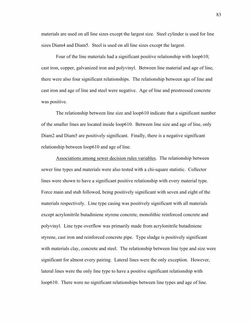
83

materials are used on all line sizes except the largest size. Steel cylinder is used for line

sizes Diam4 and Diam5. Steel is used on all line sizes except the largest.

Four of the line materials had a significant positive relationship with loop610;

cast iron, copper, galvanized iron and polyvinyl. Between line material and age of line,

there were also four significant relationships. The relationship between age of line and

cast iron and age of line and steel were negative. Age of line and prestressed concrete

was positive.

The relationship between line size and loop610 indicate that a significant number

of the smaller lines are located inside loop610. Between line size and age of line, only

Diam2 and Diam5 are positively significant. Finally, there is a negative significant

relationship between loop610 and age of line.

Associations among sewer decision rules variables. The relationship between

sewer line types and materials were also tested with a chi-square statistic. Collector

lines were shown to have a significant positive relationship with every material type.

Force main and stub followed, being positively significant with seven and eight of the

materials respectively. Line type casing was positively significant with all materials

except acrylonitrile butadiniene styrene concrete, monolithic reinforced concrete and

polyvinyl. Line type overflow was primarily made from acrylonitrile butadiniene

styrene, cast iron and reinforced concrete pipe. Type sludge is positively significant

with materials clay, concrete and steel. The relationship between line type and size were

significant for almost every pairing. Lateral lines were the only exception. However,

lateral lines were the only line type to have a positive significant relationship with

loop610. There were no significant relationships between line types and age of line.

84

Among the materials, acrylonitrile butadiniene styrene, ductile iron and cast iron

exhibited a positively significant relationship with each of the line sizes. Corrugated

metal pipe is used primarily for the smaller pipes and monolithic reinforced concrete is

for the larger pipes. Clay and polyvinyl and steel are mainly used on all pipes except the

larger sizes. Concrete and reinforced concrete pipe are mainly used on all sizes except

the smaller sizes. Only the material polyvinyl was positively significant with age of line.

Diam3 was the only line size primarily located within loop610. There were no

significant relationships between any of the diameters and age of line. As we saw with

water, the relationship between age of line and loop610 was positively significant.

Associations between decision rules variables and dependent variables.

Table 4.11 shows the relationships between the water decision rules and the dependent

variables. The relationships were tested with a logistic regression. Among line types,

only main was positively significant. This occurred in 1992 and 1995. Different

materials were significant in different years. The relationship between water capital

improvement projects and galvanized iron was significant for five of the eight years

which indicate that this material gets repaired the most. Polyvinyl followed, being

significant in four years. Note that the direction of the relationship between polyvinyl

and water capital improvement projects is negative in 1996. The reasons for that are

unclear. The materials cast iron and concrete were significant for two years. Copper

was positively significant in 1992.

The variable Diam1 had a positive significant relationship with water capital

improvement projects between 1992 and 1998 supporting Public Works’ contention that

85

smaller lines receive higher priority. The variables Diam3 and Diam5 were positively

significant in 1992. Diam2 was positively significant in 1994.

TABLE 4.11: Water Decision Rules and Dependent Variable CIP 92 CIP 93 CIP 94 CIP 95 CIP 96 CIP 97 CIP 98 CIP 99 T_MAIN L= 1.160

(.0001) L=.3347 (.3503)

L=.2539 (.4095)

L=.6366 (.0357)

L=.4319 (.2504)

L=.1028 (.7229)

L=.3088 (.4211)

L=.5881 (.1542)

T_COLL L=-.7466 (.0785)

L=.0059 (.9899)

L=-.0611 (.8826)

L=-.5677 (.2138)

L=-.3948 (.4753)

L=-.2449 (.5496)

L=-0307 (.9520)

L=.3567 (.4619)

T_HYDL L=.0413 (.8754)

L=.0689 (.8461)

L=.3368 (.2761)

L=.3546 (.2325)

L=.1427 (.7001)

L=.0062 (.9827)

L=.7569 (.0597)

L=-.3976 (.3275)

T_FIRE L=.4759 (.0727)

L=.3963 (.2661)

L=.5468 (.0773)

L=.1322 (.6535)

L=.6197 (.0993)

L=.2203 (.4475)

L=.0584 (.8785)

L=.7732 (.0611)

T_TRANS L=.5626 (.3539)

L=-13.19 (.9824)

L=13.26 (.9794)

L=-.8050 (.4425)

L=-.1998 (.8498)

L=.4605 (.4906)

L=-12.17 (.9751)

L=.8067 (.3080)

M_AC L=-.1674 (.5263)

L=.7212 (.0527)

L=-.2293 (.4563)

L=-.4307 (.1492)

L=.0058 (.9874)

L=.1745 (.5480)

L=.4459 (.2503)

L=-.2346 (.5593)

M_CI L=.7548 (.0058)

L=.5849 (.1103)

L=.5304 (.0906)

L=-.1671 (.5709)

L= 1.025 (.0119)

L=.3441 (.2392)

L=.2972 (.4387)

L=.5766 (.1624)

M_CONC L=-2.306 (.0470)

L=.0437 (.9452)

L=-.3645 (.5614)

L=1.000 (.0191)

L=.5140 (.3679)

L=-.1840 (.7409)

L=-.2504 (.7408)

L=.3567 (.5793)

M_COP L=.7101 (.0140)

L=.4993 (.1971)

L=.5911 (.0763)

L=.0922 (.7895)

L=.4850 (.2289)

L=.1521 (.6513)

L=-.1722 (.7164)

L=-.5564 (.3173)

M_DI L=.0812 (.7763)

L=-.5669 (.1913)

L=.3750 (.2423)

L=.0016 (.9959)

L=-.8817 (.0782)

L=.3308 (.2784)

L=.0209 (.9600)

L=.5336 (.1923)

M_GALV L= 1.539 (.0001)

L= 1.132 (.0021)

L= 1.307 (.0001)

L=.5829 (.0489)

L=.2673 (.4741)

L=.8431 (.0041)

L=-.0558 (.8877)

L=.7771 (.0538)

M_PC L=-.0125 (.9848)

L=.8581 (.1981)

L=-13.27 (.9779)

L=-.9544 (.3603)

L=.4490 (.5647)

L=1.009 (.0714)

L=-12.18 (.9734)

L=-.1580 (.8807

M_PVC L=.7068 (.0093)

C-.0336 (.9246)

L= 1.076 (.0013)

L=1.136 (.0004)

L=-.9907 (.0151)

L=.3692 (.2066)

L=.3204 (.4038)

L=.5996 (.1463)

M_SRC L=-.1235 (.8088)

L=.1242 (.8455)

L=-.2841 (.6520)

L=-.8702 (.2447)

L=-1.012 (.3276)

L=1.666 (.1051)

L=.3104 (.6286)

L=.8098 (.1628)

M_STL L=.9548 (.0508)

L=.0336 (.9472)

L=.2372 (.6081)

L=.8591 (.1127)

L=.5466 (.3817)

L=.2149 (.6199)

L=-.1655 (.7470)

L=-.3038 (.5578)

DIAM1 L= 1.231 (.0001)

L= 1.010 (.0095)

L=.7308 (.0224)

L=.8117 (.0087)

L=.8643 (.0292)

L= 1.175 (.0003)

L=.2972 (.4387)

L=.7506 (.0754)

DIAM2 L=.3913 (.1416)

L=.3230 (.3675)

L=.6269 (.0466)

L=.3546 (.2325)

L=-.1310 (.7236)

L=-.2465 (.3974)

L=.0597 (.0597)

L=.2461 (.5402)

DIAM3 L=.9072 (.0011)

L=.0689 (.8461)

L=.3368 (.2761)

L=.4432 (.1378)

L=.5633 (.1391)

L=-.1619 (.5772)

L=.5987 (.1285)

L=.7506 (.0754)

DIAM4 L=-.1148 (.6640)

L=.4997 (.1672)

L=.3859 (.2121)

L=-.2044 (.4894)

L=.0525 (.8871)

L=.0564 (.8456)

L=-.0929 (.8075)

L=.1316 (.7421)

DIAM5 L=.5954 (.0249)

L=.4995 (.1606)

L=-.1713 (.5890)

L=.3757 (.2034)

L=.7081 (.0578)

L=.0393 (.8938)

L=.2841 (.4573)

L=.5060 (.2064)

LOOP610 L= 1.774 (.0001)

L=.9900 (.0058)

L=.8261 (.0080)

L=-.0425 (.8948)

L=.9163 (.0141)

L=-.1031 (.7471)

L=.1473 (.7159)

L=.8202 (.0418)

AGE L= -.0060 (.5356)

L= .0249 (.0198)

L=-.0137 (.2535)

L=-.0451 (.0011)

L= .0086 (.4806)

L=-.0102 (.3547)

L=-.0184 (.2349)

L=-.0164 (.3065)

= Indicates significance at p=<.05 L=Logistic Regression

86

For five years, loop610 had a positive significant relationship with the dependent

variable. Age of line was positively significant in 1993 but negatively related in 1995.

The relationship between the sewer independent variables and the dependent

variable in Table 4.12 shows that in any given year, very few variables had a significant

effect on the dependent variable. In 1992 and 1993 lateral lines were positively

significant. No other line types demonstrated a significant relationship with sewer

capital improvement projects until collector in 1998. The nature of that relationship was

positive.

The material acrylonitrile butadiniene styrene was significant in four of the eight

years. The direction of the relationship was negative in all four years. Concrete had a

positive significant effect in 1993 and 1994. The only other material to have a

significant relationship with sewer capital improvement projects was corrugated metal

pipe in 1998 and monolithic reinforced concrete in 1997. Both of those relationships

were positive. The smaller line size (Diam1) had a positive significant relationship with

sewer capital improvement projects. The relationship between water capital

improvement projects and loop610 was positive and significant in 1992 and 1993.

Multivariate Analysis

The summarized results of water and sewer multivariate analysis are in

Table 4.13. The complete results can be found in Appendix D. The variables

transmission and collector were omitted from the water multivariate analysis. A

combination of low frequencies and concentrated locations compromised the validity of

parameters and model fit estimates.

87

TABLE 4.12: Sewer Decision Rules Relationship with Dependent Variable CIP 92 CIP 93 CIP 94 CIP 95 CIP 96 CIP 97 CIP 98 CIP 99 T_CASE L=.2903

(.4704) L=-.1681 (.7391)

L=.6450 (.1944)

L=.5926 (.1985)

L=.1219 (.8127)

L=.2952 (.4433)

L=-.3761 (.5518)

L=-.8464 (.2596)

T_COLL L=.3621 (.2597)

L=.0689 (.8461)

L=-.2737 (.5282)

L=-.3050 (.4420)

L=-.1489 (.7055)

L=.0061 (.9838)

L= 1.761 (.0015)

L=-.2572 (.5446)

T_FM L=-.2769 (.4026)

L=.3239 (.3626)

L=-.0976 (.8248)

L=-.2562 (.5312)

L=.2241 (.5699)

L=-.2589 (.4116)

L=-.2408 (.5759)

L=-.4310 (.3297)

T_LATL L= 1.238 (.0003)

L= 1.339 (.0006)

L=.5949 (.1707)

L=.1648 (.6759)

L=.3197 (.4162

L=.2491 (.4135)

L=-.1178 (.7803)

L=.4029 (.3313)

T_OF L=.2963 (.3752)

L=.3638 (.3250)

L=.0289 (.9508)

L=-.0676 (.8763)

L=-.0676 (.8763)

L=.1156 (.7234)

L=-.3187 (.5089)

L=.2994 (.4891)

T_SIPH L=-.0822 (.8507)

L=.6283 (.1297)

L=-.2942 (.6433)

L=-.1857 (.7396)

L=.9663 (.0251)

L=-.2241 (.6052)

L=.7352 (.1170)

L=.5056 (.3027)

T_SLDG L=.5119 (.3261)

L=.5300 (.3541)

L=-12.18 (.9690)

L=-.0516 (.9460)

L=.8080 (.1636)

L=-.2664 (.6727)

L=.0803 (.9164)

L=.9506 (.1042)

T_STUB L=.3621 (.2597)

L=-.4407 (.2231)

L=-.2737 (.5282)

L=-.1489 (.7055)

L=.4757 (.2362)

L=.0985 (.7459)

L=-.2526 (.5446)

L=.2640 (.5265)

M_ABS L=-.9510 (.0073)

L=-.0067 (.9848)

L=-1.467 (.0088)

L=-.1317 (.7399)

L=.3339 (.3967)

L=-.6737 (.0369)

L=.7934 (.0652)

L=-1.294 (.0113)

M_CGMP L=.6866 (.1324)

L=-1.329 (.1972)

L=.7795 (.1800)

L=.5300 (.3541)

L=-.3116 (.6803)

L=.0886 (.8618)

L=1.251 (.0135)

L=.6730 (.2435)

M_CI L=-.0608 (.8486)

L=-.2288 (.5231)

L=-.7926 (.0887)

L=.0865 (.8257)

L=-.0681 (.8627)

L=-.3746 (.2257)

L=.5199 (.2180)

L=-.5296 (.2182)

M_CLAY L=.0277 (.9404)

L=-.0702 (.8680)

L=.3492 (.4577)

L=.2568 (.5567)

L=-.4004 (.4315)

L=.1237 (.7222)

L=-.2491 (.6288)

L=.2240 (.6284)

M_CONC L=-.1335 (.6750)

L=.7330 (.0490)

L=.2964 (.4945)

L=-.1373 (.7273)

L=-.4526 (.2597)

L=.0185 (.9515)

L=.0129 (.8039)

L=-.4168 (.3233)

M_DI L=-.1382 (.6653)

L=-.3348 (.3546)

L=.0154 (.9716)

L=-.3603 (.3696)

L=.2643 (.5023)

L=-.1611 (.5982)

L=.0229 (.9559)

L=-.6966 (.1149)

M_MRC L=-.4000 (.2328)

L=-.3422 (.3585)

L=-.3076 (.4951)

L=.3673 (.3505)

L=.0557 (.8884)

L=.6723 (.0284)

L=.6229 (.1356)

L=.4499 (.2781)

M_PVC L=.1820 (.5676)

L=-.2877 (.4221)

L=-.6400 (.1555)

L=-.1258 (.7494)

L=.1835 (.6414)

L=-.5326 (.0876)

L=-.0572 (.8902)

L=.4626 (.2730)

M_RCP L=.3864 (.2291)

L=-.2877 (.4221)

L=-.4418 (.3157)

L=-.4410 (.2721)

L=.1835 (.6414)

L=-.2473 (.4186)

L=.2869 (.4913)

L=.2869 (.4913)

M_STL L=.1591 (.6907)

L=-.2910 (.5628)

L=.7558 (.1114)

L=.2460 (.6096)

L=-.2857 (.6085)

L=.0105 (.9789)

L=-.4953 (.4323)

L=-.1419 (.8011)

DIAM1 C=-.1289 (.7065)

C=-.1090 (.7753)

C=.2556 (.5630)

C=-.4484 (.3200)

C=-.2532 (.5591)

C=-.0836 (.7970)

C=-.0777 (.8609)

C=.8207 (.0487)

DIAM2 C=.0687 (.8289)

C=-.0454 (.8983)

C=-.4532 (.3034)

C=.0173 (.9649)

C=-.1373 (.7273)

C=.1108 (.7155)

C=.6325 (.1415)

C=.1029 (.8039)

DIAM3 C=.2838 (.3746)

C=-.1601 (.6531)

C=-.0643 (.8814)

C=.4987 (.2143)

C=.4987 (.2143)

C=-.5326 (.0876)

C=.2869 (.4913)

C=-.5868 (.1725)

DIAM4 C=-.1172 (.7124)

C=-.2524 (.4813)

C=-.6059 (.1787)

C=-.5705 (.1628)

C=-.0912 (.8169)

C=.2527 (.4069)

C=.3212 (.4410)

C=-.0029 (.9560)

LOOP610 P= 1.541 (.0001)

P=.9900 (.0058)

P=.4136 (.3503)

P=-.0949 (.8270)

P=.7471 (.0598)

P=.1914 (.5526)

P=-.3456 (.4737)

P=.6335 (.1311)

AGE T=-.010 (.4030)

T=.0203 (.0888)

T= .0132 (.3748)

T= .0012 (.9350)

T=-.0029 (.8488)

T=-.0133 (.2940)

T=-.0334 (.0829)

T=-.0242 (.1898)

= Indicates significance at p=<.05 L=logistic regression

88

TABLE 4.13: Decision Rules Model Multivariate Analysis Year Coefficients (p-value) Odds Ratio Confidence Intervals

Water 1992 WWO .6750 .0001 1.964 (1.478, 2.609) M-CONC -2.9636 .0057 .052 (.006, .423) M_STL 1.2530 .0246 3.501 (1.174, 10.438) DIAM5 .7096 .0202 2.033 (1.117, 3.700) LOOP610 1.7694 .0001 5.867 (3.207, 10.735) 1993 M_AC .7579 .0472 2.134 (1.010, 4.510) M_GALV 1.2185 .0012 3.382 (1.621, 7.058) AGE .0263 .0192 1.027 (1.004, 1.049) 1994 T_MAIN -1.1083 .0142 .330 (.136, .801) M_GALV 1.5074 .0001 4.515 (2.269, 8.982) M_PVC .9634 .0075 2.621 (1.294, 5.307) DIAM2 1.2877 .0041 3.624 (1.503, 8.738) 1995 M_CONC .9053 .0496 2.473 (1.002, 6.104) M-PVC .9059 .0092 2.474 (1.251, 4.892) DIAM1 1.0398 .0035 2.829 (1.407, 5.687) LOOP610 -.7714 .0382 .462 (.223, .959) AGE -.0446 .0018 .956 (.930, .984) 1996 M_GALV -1.5123 .0248 .220 (.059, 825) M_PVC -1.6432 .0004 .193 (.078, 478) DIAM3 1.0867 .0101 2.964 (1.295, 6.785) LOOP610 1.1514 .0037 3.163 (1.455, 6.875) 1997 M_GALV .8288 .0308 2.290 (1.080, 4.859) DIAM1 1.1752 .0003 3.239 (1.723, 6.088) LOOP610 -1.0229 .0093 .360 (.166, .777) 1998 WWO .4434 .0121 1.558 (1.102, 2.203) 1999 WWO .8026 .0007 2.231 (1.400, 3.555) T_HYDL -2.1817 .0002 .119 (.036, .354) T_FIRE 1.0970 .0193 2.995 (1.195, 7.508) M_COP -1.5383 .0181 .215 (.060, .769) DIAM3 1.4137 .0136 4.111 (1.337, 12.640) Sewer 1992 M_ABS -1.1281 .0048 .324 (1.48, 7.08) DIAM3 .9365 .0110 2.551 (1.239, 5.252) LOOP610 1.5040 .0001 4.499 (2.296, 8.818) 1993 T_LATL 1.3690 .0005 3.931 (1.810, 8.536) M_CONC .7649 .0454 2.149 (1.016, 4.545) AGE .0253 .0425 1.026 (1.001, 1.051) 1994 SWO .4465 .0357 1.563 (1.030, 2.371) M_ABS -1.4312 .0110 .239 (.079, .720) 1995 1996 T_SIPH 1.0304 .0184 2.802 (1.190, 6.597) LOOP610 .8086 .0445 2.245 (1.020, 4.939)

89

TABLE 4.13: continued Year Coefficients (p-value) Odds Ratio Confidence Intervals

1997 SWO .4362 .0023 1.547 (1.168, 2.048) M_MRC .6565 .0361 1.928 (1.043, 3.563) DIAM3 -.6618 .0391 .516 (.275, .967) 1998 T_COLL 1.6887 .0025 5.413 (1.810, 16.186) M_CGMP 1.0592 .0417 2.884 (1.041, 7.993) 1999 SWO .5063 .0129 1.659 (1.113, 2.472) M_ABS -1.4385 .0062 .237 (.085, .664) DIAM1 1.0053 .0206 2.733 (1.167, 6.401)

Water

Significant for five years in the simple model, with the addition of the decision

rules variables water work orders is only positively significant for three (1992, 1998 &

1999). A look at the results shows that in 1992, water work orders, two types of

material, larger size lines and lines inside of loop610 significantly predict the likelihood

of a capital improvement project. All variables but concrete were positive. The

strongest variables, as indicated by the Odds Ratio, are loop610 and steel. The weakest

variable is the material concrete. Concrete also contributes inversely to the model. In

1993, galvanized iron, age of line and asbestos cement are the best predictors. Three

variables were positively significant in 1994; galvanized iron and polyvinyl and Diam2

The fourth variable, main, was negatively significant. Galvanized iron was the strongest

predictor followed by Diam2, polyvinyl and main. In 1995, the variable Diam1 has the

strongest power, loop610 and age of line are the weakest. Loop610 and age of line

contributed negatively to the model. In fact, according to the confidence intervals, these

two variables, along with concrete, get close to making no significant contribution to the

model. In the following year, we see the materials polyvinyl and loop610 are again

90

significant, although polyvinyl has a negative relationship and loop610 is positive.

These variables are accompanied by galvanized iron and Diam3. In 1997, the variables

Diam3, galvanized iron and loop610 reappear. Water work orders were again positively

significant in 1998 and 1999. In 1999, water work orders was joined by hydrant, fire

line, copper and Diam3.

Although water work orders have not been significant in every year, they have

been significant 37 percent of the time, therefore, we can reject the null hypothesis 3a.

Water work orders have had a significant effect on predicting the likelihood of a capital

improvement project when taken into consideration with technical factors.

Sewer

Sewer work orders remained significant in the same three years (1994, 1997 and

1999) that they were in the simple model. A review of the years shows the significant

variables. In 1992, Diam3 and loop610 are all positively significant with the variable

loop610 having the strongest degree of predictability. The variable acrylonitrile

butadiniene styrene is also significant but its relationship is negative, and, according to

the Odds Ratio, its contribution to the model is the weakest. In 1993, lateral, concrete

and age of line were able to predict the likelihood of a capital improvement project.

The year 1994 is the first year we see the significance of sewer work orders, it is

joined by the variable acrylonitrile butadiniene styrene. No variables were significant in

1995. In 1996, the predicting variables were siphon and loop610. Two new variables

joined sewer work orders in predicting the likelihood of a capital improvement project in

1997. The following year we see that collector and corrugated metal pipe are

91

significant. In 1998, sewer work orders and acrylonitrile butadiniene styrene are joined

by Diam1.

Because sewer work orders was also significant at least 37 percent of the time,

we reject null hypothesis 3b. When taken in consideration with technical factors, sewer

work orders had a significant effect on the selection of sewer related capital

improvement projects.

Adding the significant decision rules variables to the variables found to be

significant in the previous models results in the following (Table 4.14):

TABLE 4.14: Cumulative List of Significant Variables with Decision Rules Significant Variables: Water Sewer

Water work orders (WWO) Sewer work orders (SWO) Theory: Class Bias Percent nonwhite (NONWHITE)

Percent income (INC) Cost of housing (COST)

Cost of housing (COST) Percent nonwhite (NONWHITE) Percent income (INC)

Theory: Decision Rules Significant Variables: Main (MAIN)

Hydrant (HYDL) Fire line (FIRE) Concrete (CONC) Steel (STL) Acrylonitrile (ABS) Galvanized (GALV) Polyvinyl (PVC) Copper (COP) Diam1 (DIAM1) Diam2 (DIAM2) Diam3 (DIAM3) Diam5 (DIAM5) Loop610 (LOOP610) Age of line (AGE)

Lateral (LATL) Siphon (SIPH) Collector (COLL) Corrugated metal (CGMP) Asbestos cement (AC) Concrete (CONC) Monolithic reinforced pipe (MRC) Diam1 (DIAM1) Diam3 (DIAM3) Loop610 (LOOP610) Age of line (AGE)

92

Model Fit

The addition of the water decision rules variables is a better fit over the intercept

only model for every year (see Appendix D). As calculated by the Likelihood Ratio, the

range of improvement is between 6.8 in 1998 and 85.9 in 1992. In every year but 1998,

the Likelihood Ratio and Score values indicate that the model significantly improved by

adding decision rules variables. In all but one year, 1998, the Decision Rules model is

an improvement over the simple model. In that year, the results of the two multivariate

analysis are the same.

The addition of the decision rules variables to the sewer model resulted in a

decrease in the –2 Log Likelihood values in seven of the eight years. The range of

improvements were a low of 8.4 in 1996 to a high of 33.5 in 1992. In these years, the

improvements were shown to be significant. In 1995, no variables were significant thus

no change in the –2 Log L. A comparison of this model to the simple model show that

the Decision Rules Model seems to be a better in every year except 1995.

Political Influence

Univariate Analysis

Analyzing the political influence model differed from the previous models.

Political data was only available by precincts. Few census tracts and voter precinct share

the same boundaries. Seventeen percent (17 percent) of the census tracts were perfectly

aligned with precinct borders, the remaining precincts were divided between tracts.

93

Adjustments were made and the number of census tracts studied for this model is 64.

That number represents those precinct boundaries that closely match census boundaries.

There are five variables representing the political model, stable (STABLE),

percent vote (VOTE), percent active (ACTIVE), tenure (TEN), and DIST. The

descriptive statistics are shown in Table 4.15.

Percent active is the number of work orders per census population. The range of

values for this variable is 0 to 13.04. In general, less than 13 percent of the census tract

population contacts the city to complain. Note that the maximum increases steadily over

the eight-year period. This may be due to an increasing awareness of the Customer

Response Center. The values of percent active were dichotomized based on the median

value.

Percent vote represents the number of registered voters per census tract

population. Notice that the yearly maximum often exceeds the population. This is due

to the nature of raw data and characteristics of voters. The records are updated every

two years. Oftentimes, the voter has moved but has yet to notify Harris County. Also,

the number of voters increase but the denominator is based on census information that is

static as of 1990. To accommodate this, the values for percent vote were dichotomized

based on the median value.

Tenure is the number of years the council member has been in office. The range

is 1 to 6. Prior to 1993, there were no term limits so years served over six were

classified as six. In 1992, of the eight council members, six (or 75 percent) had served

six or more years. In DistE, the council member was serving his 28th year. As expected,

the mean years in office decreased with 64 percent serving their first year. Tenure then

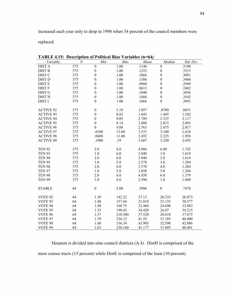
94

increased each year only to drop in 1998 when 54 percent of the council members were

replaced.

TABLE 4.15: Description of Political Bias Variables (n=64) Variable N Min Max Mean Median Std. Dev

DIST A 375 0 1.00 .1146 0 .3190 DIST B 375 0 1.00 .1253 0 .3315 DIST C 375 0 1.00 .1066 0 .3091 DIST D 375 0 1.00 .1386 0 .3460 DIST E 375 0 1.00 .0960 0 .2949 DIST F 375 0 1.00 .0613 0 .2402 DIST G 375 0 1.00 .1040 0 .3056 DIST H 375 0 1.00 .1466 0 .3542 DIST I 375 0 1.00 .1066 0 .3091 ACTIVE 92 375 0 5.19 1.057 .8700 .0651 ACTIVE 93 375 0 8.82 1.645 1.445 1.542 ACTIVE 94 375 0 9.05 2.789 2.535 2.117 ACTIVE 95 375 0 8.14 2.888 2.815 2.093 ACTIVE 96 375 0 9.08 2.763 2.475 2.017 ACTIVE 97 375 .0100 13.04 3.331 3.100 2.624 ACTIVE 98 375 .0400 11.08 2.452 2.225 1.958 ACTIVE 99 375 .1900 .19 3.687 3.250 2.692 TEN 92 375 2.0 6.0 4.986 6.00 1.742 TEN 93 375 1.0 6.0 2.040 1.0 1.614 TEN 94 375 2.0 6.0 3.040 2.0 1.614 TEN 95 375 1.0 5.0 2.578 3.0 1.284 TEN 96 375 2.0 6.0 3.578 4.0 1.284 TEN 97 375 1.0 5.0 3.858 5.0 1.284 TEN 98 375 2.0 6.0 4.858 6.0 1.379 TEN 99 375 1.0 6.0 2.594 1.0 1.840 STABLE 64 0 2.00 .3906 0 .7478 VOTE 92 64 1.39 142.22 27.13 20.235 26.873 VOTE 93 64 1.48 157.64 31.019 23.135 30.577 VOTE 94 64 1.50 169.75 32.466 24.690 32.083 VOTE 95 64 1.53 190.43 34.420 26.07 34.215 VOTE 96 64 1.57 210.380 37.528 28.610 37.073 VOTE 97 64 1.70 236.13 41.55 31.185 40.400 VOTE 98 64 1.68 156.34 43.905 32.590 42.886 VOTE 99 64 1.63 238.160 41.177 31.095 40.401

Houston is divided into nine council districts (A-I). DistH is comprised of the

most census tracts (15 percent) while DistE is comprised of the least (10 percent).

95

The variable stable represents those precincts that had not been redistricted

during the study period. Less than 25 percent of the precincts had not been redistricted.

The values associated with stable range from 0 to 3. The value 0 indicates there have

been changes, 1 represents a stable tract, 2 indicates that the census tract is comprised of

two or more precincts where at least one of them is stable. See Appendix A for

description of the political influence variables after adjustments were made.

Bivariate Analysis

Associations between work orders and political bias independent variables.

Table 4.16 shows the results of the relationship between work orders and the

independent variables. Because it is calculated using work orders in the denominator,

the relationship between percent active and water work orders is always significant. The

Cramer’s V statistic indicates that the relationship is stronger in the early years and

decreases over time.

Among the districts, DistA was positively significant in 1994 while DistI was

positively significant in 1992. DistE displayed the longest significant relationship with

water work orders. It was positively related in 1992 through 1994. DistF and DistG

were each positively significantly related to work orders in 1999 and 1998, respectively.

The final district to have a significant relationship with work orders was DistI in 1992

and 1993.

96

TABLE 4.16: Bivariate Political and Water Work Orders WWO 92 WWO 93 WWO 94 WWO 95 WWO 96 WWO 97 WWO 98 WWO 99

Water ACTIVE C=.6157

(.0001) C=.5871 (.0001)

C=.5990 (.0001)

C=.4979 (.0001)

C=.4377 (.0001)

C=.3782 (.0001)

C=.2592 (.0001)

C=.3993 (.0001)

TEN B=-.0082 (.8616)

B=.1175 (.0101)

B=.1197 (.0088)

B=-.113 (.0125)

B=-.058 (.2012)

B=-.011 (.8066)

B=.0644 (.1567)

B=-.0222 (.6249)

DISTA K=6.8006 (.0785)

K=2.3061 (.5114)

K=7.9712 (.0466)

K=6.4922 (.0900)

K=7.3396 (.0618)

K=1.9384 (.5853)

K=4.0546 (.2556)

K=3.6670 (.2957)

DISTB K=13.0481 (.0045)

K=4.8547 (.1828)

K=6.0409 (.1096)

K=1.8308 (.6082)

K=7.6188 (.0546)

K=5.2373 (.1552)

K=2.3765 (.4980)

K=2.3448 (.5040)

DISTC K=3.0525 (.3836)

K=3.1869 (.3637)

K=4.5393 (.2088)

K=1.7436 (.6273)

K=1.6679 (.6441)

K=2.8821 (.4102)

K=1.9345 (.5861)

K=1.0250 (.7952)

DISTD K=2.6368 (.4511)

K=2.2020 (.5315)

K=7.3228 (.0623)

K=4.9224 (.1776)

K=6.3231 (.0969)

K=3.0312 (.3868)

K=.3275 (.9548)

K=3.2489 (.3548)

DISTE K=18.5267 (.0003)

K=22.7197 (.0001)

K=17.3540 (.0006)

K=7.7642 (.0511)

K=7.3457 (.0617)

K=2.4980 (.4757)

K=4.7653 (.1898)

K=4.1657 (.2441)

DISTF K=3.9855 (.2630)

K=1.5153 (.6787)

K=.5556 (.9065)

K=.4069 (.9388)

K=.2234 (.9737)

K=3.1583 (.3679)

K=3.7472 (.2901)

K=8.8421 .0315

DISTG K=.9272 (.8189)

K=3.4714 (.3245)

K=5.2042 (.1574)

K=5.4956 (.1389)

K=1.4430 (.6955)

K=1.7211 (.6323)

K=8.0301 (.0454)

K=6.9645 (.0730)

DISTH K=1.3307 (.7218)

K=3.2934 (.3486)

K=2.7317 (.4349)

K=3.1976 (.3622)

K=1.9043 (.5925)

K=3.7196 (.2934)

K=5.6255 (.1313)

K=1.7428 (.6275)

DISTI K=13.2895 (.0041)

K=7.9893 (.0462)

K=5.5561 (.1353)

K=6.1014 (.1068)

K=3.3315 (.3433)

K=4.1173 (.2491)

K=1.2125 (.7500)

K=1.0997 (.7771)

STABLE B=.1093 (.0201)

B=.0926 (.0491)

B=.0865 (.0660)

B=.1077 (.0220)

B=.0231 (.6234)

B=.0913 (.0524)

B=.0943 (.0449)

B=.0160 (.0242)

VOTE B= .1401 (.183)

B=.1422 (.1770)

B=.1336 (.2044)

B=.1985 (.0591)

B=.2141 (.0426)

B=.2058 (.0522)

B=.1526 (.1493)

B=.1477 (.1617)

SWO92 SWO93 SWO94 SWO95 SWO96 SWO97 SWO98 SWO99 Sewer ACTIVE C=.6671

(.0001) C=.6581 (.0001)

C=.5926 (.0001)

C=.5550 (.0001)

C=.5686 (.0001)

C=.5463 (.0001)

C=.5308 (.0001)

C=.5674 (.0001)

TEN .B=-.154 (0001)

B=.255 (.0001)

B=.229 (.0001)

B=-.220 (.0001)

B=-.219 (.0001)

B=-.135 (.0028)

B=-.055 (.2225)

B=.1409 (.0020)

DISTA K=5.6833 (.1281)

K=8.6662 (.0341)

K=9.0566 (.0285)

K=4.3088 (.2300)

K=4.2972 (.2311)

K=4.0669 (.2543)

K=2.1913 (.5337)

K=.7469 (.8621)

DISTB K=5.7823 (.1227)

K=8.5150 (.0365)

K=7.8517 (.0492)

K=3.2065 (.3609)

K=8.5268 (.0363)

K=2.7603 (.4301)

K=.6707 (.8801)

K=.7878 (.8524)

DISTC K=.5735 (.9025)

K=2.0383 (.5645)

K=4.0250 (.2588)

K=3.9772 (.2639)

K=4.5099 (.2114)

K=7.0617 (.0700)

K=5.8154 (.1209)

DISTD K=20.9128 (.0001)

K=23.3849 (.0001)

K=29.3743 (.0001)

K=26.6685 (.0001)

K=28.862 (.0001)

K=30.6584 (.0001)

K=9.7985 (.0204)

K=13.4837 (.0031)

DISTE K=16.854 (.0008)

K=8.9789 (.0300)

K=15.4399 (.0015)

K=13.3732 (.0039

K=13.5510 (.0036)

K=7.9746 (.0465)

K=12.1829 (.0068)

K=13.0641 (.0045)

DISTF K=2.6177 (.4544)

K=2.9144 (.4050)

K=.8046 (.8484)

K=1.2244 (.7471)

K=1.4258 (.6995)

K=.3825 (.9438)

K=3.5927 (.3089)

K=3.9893 (.2626)

DISTG K=12.0359 (.0073)

K=14.2730 (.0026)

K=15.1450 (.0017)

K=15.6708 (.0013)

K=19.2771 (.0002)

K=15.1732 (.0017)

K=8.8459 (.0314)

K=8.6916 (.0337)

DISTH K=14.5430 (.0023)

K=10.6147 (.0140)

K=23.0609 (.0001)

K=17.4725 (.0006)

K=7.2005 (.0658)

K=8.2579 (.0410)

K=7.3887 (.0605)

K=6.4751 (.0906)

DISTI K=13.6512 (.0034)

K=21.3347 (.0001)

K=14.9056 (.0019)

K=17.3568 (.0006)

K=10.9084 (.0122)

K=15.9283 (.0012)

K=8.8842 (.0309)

K=5.4420 (.1422)

STABLE B=.1229 (.0092)

B=.1167 (.0132)

B=.1315 (.0053)

B=.1441 (.0022)

B=.0955 (.0424)

B=.1195 (.0110)

B=.1535 (.0011)

B=.1225 (.0093)

VOTE B=.0293 (.7821)

B=.0994 (.3487)

B=.0339 (.7490)

B=.0722 (.4947)

B=.2169 (.0402)

B=1731 (.1024)

B=1400 (.1896)

B=.1836 (.0844)

= Indicates significance at p=<.05 C=chi-square/Cramer’s V B=Kendall tau b K=Kruska-Wallis

97

Tenure has a significant, albeit weak, relationship with water work orders

between 1993 and 1995. In 1993 the relationship is positive, in 1995 the relationship is

negative. The variables stable and water work orders exhibit a significant relationship in

five of the eight years. These relationships are not strong but are consistently positive.

Percent vote was only significantly positive in 1996.

The level of association between sewer work orders (SWO) and percent active is

significant in every year. The relationship between tenure and sewer work orders is

significant for seven of the eight years studied. The direction of the relationship varies

between years. In 1992 and between 1995 and 1997, the relationship was negative in

1993, 1994 and 1999 the relationship was positive. The reason for the change in signs is

unclear.

The variable stable has a significant relationship with sewer work orders during

the entire study period. During each of the years, the relationship was positive. As was

the case with water, the variable percent vote was only significant in 1996. The

relationship was positive. Surprisingly, DistD and DistE and DistG were positively

significant with sewer work orders for all eight years. DistI was positively significant

six of the eight years, DistH for five. It seems that sewer work orders are more evenly

distributed across the districts over the years than water work orders.

Associations among political variables. The results of the analysis among the

political variables can be found in Appendix E. Beginning with water, tenure was

positively significantly related with all districts in every year. Tenure was also positive

and significant related with percent active in 1998. The variables percent active and

percent vote were positive and significantly related every year except 1996-1998.

Percent active and DistH displayed a significant relationship in 1995, 1996-1998. The

98

only other significant relationship with percent active was the positive relationship with

DistD in 1997 and the positive relationships with DistD, DistE and DistH in 1998.

Percent vote was only significant with DistH. This positive relationship occurred in

1997 and 1998.

Among the sewer variables, the results were similar. Tenure was significantly

and positively related to every district. Tenure was also significantly related to percent

active. In 1992, the relationship was negative; in 1992 and 1993 it was positive. The

variables percent active and percent vote were significant four of the eight years. In

each of the significant years, the relationship is positive. Percent active and stable were

significantly and positively related in 1998 and 1999. Only two districts were

significantly related to percent active. DistD was positive in 1992, 1993 and 1995.

DistG was positive in 1995 and 1997 through 1999.

Associations between political variables and dependent variables. As reflected in

Table 4.17, few of the political variables have a significant relationship with the

dependent variable. Beginning with water, the results of the chi-square analysis

indicated that there is a significantly positive relationship between percent active and

capital improvement project in 1992, 1995 and 1998. The Cramer’s V value indicates

that the relationship is relatively weak. Stable was significant and positive in 1992 and

1995. The years 1992, 1994 and 1997 were the only years where council districts were

significantly related to water capital improvement projects. In 1992, DistA, DistB and

DistH were most likely to receive a capital improvement project. In 1994, it was DistA,

DistB, DistC and DistH. By 1997, only DistG was significantly, albeit negatively,

related to the dependent variable.

99

TABLE 4.17: Bivariate Political Independent and Dependent Variable CIP 92 CIP 93 CIP 94 CIP 95 CIP 96 CIP 97 CIP 98 CIP 99

Water ACTIVE L=.7200

(.0081) L=.5967 (.1033)

L=.5427 (.0834)

L=.6366 (.0357)

L=.3038 (.4146)

L=.3692 (.2066)

L=.9459 (.0219)

L=-.3861 (.3417)

TEN L=.0470 (.5475)

L=-.0173 (.8775)

L=-.0274 (.7785)

L=-.0164 (.8864)

L=.0717 (.6161)

L=-.2284 (.0216)

L=.1719 (.2579)

L=-.1121 (.3276)

DISTA L=-1.233 (.0444)

L=-.0041 (.9941)

L=.8227 (.0393)

L=-.2744 (.5834)

L=.3963 (.4428)

L=.6334 (.1082)

L=-1.391 (.1769)

L=-1.272 (.2178)

DISTB L=-.1475 (.7207)

L=.4113 (.3899)

L=-2.064 (.0435)

L=.5565 (.1552)

L=-.8175 (.2742)

L=-.2062 (.6563)

L=-.7419 (.3220)

L=.7606 (.1220)

DISTC L=-1.595 (.0307)

L=.3732 (.4686)

L=-1.131 (.1274)

L=-.4568 (.4053)

L=-.6253 (.4046)

L= -.2287 (.6485)

L=-.0780 (.9019)

L=-.4267 (.5718)

DISTD L= .4211 (.2310)

L=-1.791 (.0807)

L=-.6639 (.2228)

L=-1.118 (.0684)

L=-.4769 (.4460)

L= .2063 (.6052)

L=-.0493 (.9298)

L= .0834 (.8824)

DISTE L=-.1707 (.7153)

L=-.6061 (.4192)

L=-.5464 (.3809)

L=-.0465 (.9268)

L=-.5011 (.5054)

L=-.0934 (.8533)

L=-.4256 (.5724)

L=-1.067 (.3022)

DISTF L=.4436 (.3695)

L=-.8551 (.4101)

L=-1.245 (.2286)

L=.5410 (.3060)

L=.8907 (.1274)

L=.1944 (.7331)

L=.9712 (.0978)

L=.7179 (.2725)

DISTG L=-.7790 (.1530)

L=-.7005 (.3495)

L=-1.845 (.0717)

L=-.1492 (.7668)

L=-.1253 (.8427)

L=-2.005 (.0500)

L= .6040 (.2474)

L=-1.159 (.2620)

DISTH L= 1.103 (.0005)

L= .7941 (.0575)

L=2.095 (.0001)

L=.0138 (.9734)

L=.3258 (.4948)

L=-.2149 (.6199)

L=-.1200 (.8297)

L=.5559 (.2546)

DISTI L=.2456 (.5431)

L=.3732 (.4686)

L=-.3336 (.5447)

L= .6265 (.1276)

L=.4884 (.3463)

L=.5761 (.1600)

L=.5718 (.2727)

L=.0494 (.9381)

STABLE L=.7051 (.0238)

L=-10.29 (.9650)

L=-.3175 (.5734)

L=.8024 (.0111)

L=-10.28 (.9665)

L=-.1459 (.7555)

L=.2593 (.5791)

L=-.3613 (.6442)

VOTE L=.1755 (.5779)

L=.1632 (.6380)

L=-.2484 (.6123)

L=-.4806 (.1306)

L=-.5788 (.3276)

L=-.1323 (.7537)

L=-.0410 (.9273)

L=-.1094 (.7575)

Sewer ACTIVE L=.0162

(.9594) L=-.0101 (.9773)

L=.6968 (.1220)

L=.2065 (.6000)

L=.3511 (.3761)

L=.0431 (.8872)

L=-.2297 (.5816)

L=.1143 (.7826)

TEN L=.0135 (.8838)

L=-.0173 (.8775)

L=.0983 (.4191)

L=.1802 (.2344)

L=-.0047 (.9753)

L=-.2150 (.0388)

L= .2167 (.2043)

L=-.1327 (.2702)

DISTA L=-1.858 (.0697)

L=-.0041 (.9941)

L= 1.100 (.0296)

L= .5697 (.2756)

L=-.0823 (.8967)

L=.4563 (.2832)

L=-1.185 (.2514)

L=-1.185 (.2514)

DISTB L=.2895 (.5148)

L=.4113 (.3899)

L=-12.24 (.9597)

L= .7108 (.1466)

L=-.6612 (.3787)

L=-.8972 (.1460)

L=-.5287 (.4737)

L=.8673 (.0809)

DISTC L=-1.028 (.1666)

L=.3732 (.4686)

L=-1.007 (.3308)

L=.0054 (.9932)

L=-.4692 (.5336)

L=-.3589 (.5143)

L=.1429 (.8232)

L=-1.101 (.2869)

DISTD L= .6725 (.0885)

L=-1.791 (.0807)

L=.2880 (.6143)

L=-1.537 (.1354)

L=-.3146 (.6176)

L=.3648 (.3652)

L=-.1771 (.7801)

L=-.1771 (.7801)

DISTE L=-.4418 (.4797)

L=-.6061 (.4192)

L=.3716 (.5649)

L=-.3444 (.6485)

L=-.3444 (.6485)

L=-.2278 (.6806)

L=-.2129 (.7791)

L=-.9802 (.3440)

DISTF L= .7732 (.1466)

L=-.8551 (.4101)

L=-.3830 (.7142)

L=-.6030 (.5627)

L= 1.056 (.0729)

L=.3372 (.5557)

L=1.1995 (.0436)

L= .8112 (.2170)

DISTG L=-13.33 (.9667)

L=-.7005 (.3495)

L=-.9786 (.3451)

L=.0364 (.9543)

L=.0364 (.9543)

L=-1.869 (.0681)

L=.8433 (.1126)

L=-1.072 (.3000)

DISTH L= .5931 (.1311)

L= .7641 (.0575)

L=.5175 (.3271)

L=-.3845 (.5411)

L=.2558 (.6204)

L=.1193 (.7748)

L=-.7189 (.3392)

L=.6626 (.1789)

DISTI L= .5055 (.2617)

L=.3732 (.4686)

L=-.2394 (.7526)

L=.3645 (.5211)

L=.3645 (.5211)

L=.7333 (.0763)

L=.1429 (.8232)

L=.1429 (.8232)

STABLE L= .6073 (.0753)

L=-10.29 (.9650)

L=-10.23 (.9715)

L=.7951 (.0284)

L=-10.26 (.9686)

L=-11.37 (.9723)

L=.3731 (.4257)

L=-.3128 (.6887)

VOTE L=.0000 (.1735)

L=-.0001 (.6587)

L=-.0005 (.7518)

L=-.0009 (.2295)

L=-.0007 (.3802)

L=-.0006 (.4846)

L=.0001 (.7560)

L=-.0002 (.5982)

= Indicates significance at p=<.05 L=Logistic Regression

100

For sewer, the variable stable is significant and positive in 1995. Tenure had a

negatively significant relationship with sewer capital improvement projects in 1997.

Only two of the nine districts were likely to receive a sewer capital improvement project.

DistA and DistE were significantly and positively related for one year; DistA in 1994

and DistF in 1998.

Multivariate Analysis

The results of the multivariate analysis are shown in Table 4.18. The decision

was made to omit percent active and percent vote from the multivariate analysis.

Percent active was omitted from the multivariate analysis due to its strong relationship

with work orders. Because percent active is calculated using work orders, the presence

of both variables in the model would be repetitive.

Percent vote’s presence in the model compromised the validity of parameters and

model fit estimates. This occurred because the variable is not present for every census

tract. Recall that there are 64 tracts that contain values for the variable percent vote.

That is less than a fifth of the study population. Therefore, the final multivariate analysis

for the political model includes the nine districts, tenure, work orders and stable.

Water work orders from DistH significantly predicted the likelihood of a capital

improvement project in 1992. The Odds Ratio for those variables indicate that DistH is

the stronger predictor. The next year with a significant variable is 1994 with the

variables DistH and DistA. In 1995, stable is the significant variable. In 1997, work

orders is again significant. DistG has a negative effect on capital improvement project

selection. In the final two years of the study, water work orders is the only variable that

101

significantly predicts the likelihood of a capital improvement project. In those two

years, the strength of the variable is similar.

Based on the results of the multivariate analysis, we can reject null hypothesis 4a.

Water work orders, when analyzed with political variables has significantly affected the

selection of capital improvement projects. However, we have to acknowledge that water

work orders was significant only 50 percent of the time.

TABLE 4.18: Political Model Multivariate Analysis Estimate (p-value) Odds Ratio Confidence Intervals

Water 1992 WWO .7216 .0001 2.058 (1.567, 2.702) DISTH 1.1526 .0007 3.166 (1.626, 6.165) 1993 1994 DISTA 1.5980 .0003 4.943 (2.073, 11.789) DISTH 2.4617 .0001 11.725 (5.616, 24.497) 1995 STABLE .8024 .0111 2.231 (1.201, 4.143) 1996 1997 WWO .3434 .0116 1.410 (1.080, 1.841) DISTG -2.0769 .0429 .125 (.017, .936) 1998 WWO .4434 .0121 1.558 (1.102, 2.203) 1999 WWO .5359 .0069 1.709 (1.159, 2.521) Sewer 1992 1993 1994 SWO .5190 .0178 1.680 (1.094, 2.581) DISTA 1.2523 .0160 3.498 (1.263, 9.693) 1995 STABLE .7951 .0284 2.215 (1.088, 4.509) 1996 1997 SWO .4201 .0025 1.522 (1.159, 2.000) 1998 DISTF 1.1995 .0436 3.318 (1.035, 10.638) 1999 SWO .5268 .0078 1.694 (1.148, 2.497)

102

For sewer work orders, the results are simple. There were only three years when

variables significantly predicted the likelihood of a capital improvement project (1994,

1997 and 1998). The strength of the relationship between sewer work orders and the

dependent variable is relatively consistent. There is less than a .15 difference in the

Odds Ratios with the strongest relationship in 1999 and the weakest in 1997. In 1994,

sewer work orders is accompanied by the stronger Predictor DistA. In 1995, the

significant variable is stable. In 1998, the variable is DistF.

In addition to sewer work orders, in 1994 DistA contributed to the prediction of

the dependent variable. As calculated by the Odds Ratio, its contribution is three times

stronger than sewer work orders. In 1998, DistF is the significant predictor. Based on

the results of the multivariate analysis, we can reject the null hypothesis 4b. Sewer work

orders, when analyzed with political variables has significantly affected the selection of

capital improvement projects.

Adding the significant variables that represent the Political Influence theory to

the other variables produces the following list of variables we may expect to see in the

full model (Table 4.19).

103

TABLE 4.19: Cumulative List of Significant Variables with Political Influence Significant Variables: Water Sewer

Water work orders (WWO) Sewer work orders (SWO) Theory: Class Bias Percent nonwhite (NONWHITE)

Percent income (INC) Cost of housing (COST)

Cost of housing (COST) Percent nonwhite (NONWHITE) Percent income (INC)

Theory: Decision Rules Significant Variables: Main (MAIN)

Hydrant (HYDL) Fire line (FIRE) Concrete (CONC) Steel (STL) Acrylonitrile (ABS) Galvanized (GALV) Polyvinyl (PVC) Copper (COP) Diam1 (DIAM1) Diam2 (DIAM2) Diam3 (DIAM3) Diam5 (DIAM5) Loop610 (LOOP610) Age of line (AGE)

Lateral (LATL) Siphon (SIPH) Collector (COLL) Corrugated metal (CGMP) Asbestos cement (AC) Concrete (CONC) Monolithic reinforced pipe (MRC) Diam1 (DIAM1) Diam3 (DIAM3) Loop610 (LOOP610) Age of line (AGE)

Theory: Political Influence Significant Variables: DistA (DISTA)

DistG (DISTG) DistH (DISTH) Stable (STABLE)

DistA (DISTA) DistE (DISTE) Stable (STABLE)

Model Fit

The addition of the political influence variables to the water model proved to be

an improvement. A look at the Likelihood Ratios and Score values, in Table 4.20,

indicate that in the years that we saw significant variables, we also experienced a

significant model fit. Comparing the fit of the political model with the simple model, we

see that the political bias model is an improvement. However, in 1993, the improvement

is by a mere 5.377 and in 1996, there is no improvement. Given this small difference, it

is correct to expect that there isn’t a significant difference in each year. In fact, the years

where the political model is a significantly better fit is in 1992, 1997, 1998 and 1999. Is

104

the political model an improvement over the simple model? Yes, in some years,

specifically in 1992, 1994, 1995 and 1997. The –2 Log Likelihood values were the same

in 1998 and 1999 where the multivariate results were the same. In the remaining years,

there were no significant variables for the Political model.

TABLE 4.20: Political Model Fit Comparisons (n=375) 2-Log Likelihood Likelihood Ratio Score Value

Intercept Only

With Covariates

chi-Square

p-value chi-Square

p-value

Water 1992 363.941 321.284 42.656 .0001 41.3119 .0001 1993 232.637 227.259 5.377 .0204 3.9175 .0478 1994 290.739 243.712 47.027 .0001 56.9163 .0001 1995 309.119 303.457 5.6618 .0173 7.6683 .0056 1996 218.704 1997 316.163 302.218 13.9454 .0009 11.6181 .0030 1998 209.077 202.221 6.8556 .0088 6.6573 .0099 1999 194.086 185.930 8.1568 .0043 7.8526 .0051 Sewer 1992 275.194 1993 232.637 1994 172.965 162.643 10.322 .0057 10.8384 .0044 1995 199.160 195.376 3.7839 .0517 5.7063 .0169 1996 199.160 1997 294.605 284.760 9.746 .0018 9.5296 .0020 1998 183.698 180.378 3.3198 .0685 4.5294 .0333 1999 183.698 175.639 8.0581 .0045 7.6989 .0055

Sewer results resemble water. There is a model improvement when we add the

political variables to the intercept-only model in five of the eight years. The range in

difference is a low of 3.31 in 1998 and a high of 10.3 in 1994. In the remaining years,

no significant variables were detected. A comparison with the simple work order model

reveals that the political influence is a better fit but only in 1994.

105

The simple and three theory-based models indicate that for both water and sewer,

work orders retained some power of predictability. However, the years and the degree

varied. The next step, to be addressed, in Chapter V, is to determine if work orders,

when taken into consideration with all the variables discussed in this chapter, have a

significant effect on the selection of capital improvement projects. A discussion of the

findings from this chapter and Chapter V will be in Chapter VI.

106

CHAPTER V

FULL MODEL ANALYSIS

Introduction

This chapter will discuss the interaction between variables outside of their

theoretical boundaries. It will then present the results of the bivariate and multivariate

analysis; determining which variables, if any, have a significant effect on the selection of

capital improvement projects. This chapter concludes by evaluating the model fit and

discussing which model best fits the data.

Bivariate Analysis

Water

As was done with the previous bivariate analysis, different tests were run based

on the variable types. The results of the analysis are in Appendix F.

Decision rules and class bias variables. Because the decision rules variables are

comprised primarily of technically oriented variables, one would not expect there to be

many statistically significant relationships between decision rules and class bias

variables. For the most part, that expectation holds true. Only the material concrete was

positive and significantly related to percent ownership. Line size showed a few more

significant interactions. The variable Diam3 was significantly yet negatively related

with housing cost. Diam5 is positive and significantly related to percent nonwhite. The

107

variable loop610 was shown to be significantly related to housing cost (negative) and

INC (positive). According to the p-values and direction of the relationship, it would

seem that higher income, lower cost census tracts are located within the central city. The

variable age of line was significantly related to percent nonwhite, housing cost and

income. This indicates that tracts with older lines are comprised of higher percentages

of non-whites. Via the direction of the relationship with housing cost and income,

higher housing costs and people with higher incomes are associated with those tracts

with newer or newly replaced lines.

Class bias and political variables. Few statistically significant relationships

existed between class bias and political variables. In two years, 1995 and 1997, percent

active had a positive relationship with percent nonwhite. In those two years, which are

election years, higher percentages of nonwhites are associated with higher percentages

of phone calls.

In 1993, 1994 and again in 1999 tenure and percent nonwhite were significantly

and negatively related. The remainder of the time, the significant relationships between

the variables were positive. Housing cost and tenure were also significant in every year

except in 1997 and 1998. The nature of the relationships vary between the years. While

it is positive a majority of the time, the relationship is negative in 1995 and 1996.

Reasons for these sign changes are unclear. The relationships between income and

tenure almost mirror the relationship between housing cost and tenure, except in 1994.

There were many statistically significant relationships between council districts

and the class bias variables. Council DistA had a positive relationship with housing cost

and DistB was significant with high percentages of percent nonwhite in high housing

108

cost, high income census tracts. DistD was negatively significant with housing cost

while DistF was significant with percent nonwhite and percent ownership. Both DistG

and DistI were significantly related with percent nonwhite but in low cost, high income

census tracts. DistH was significantly related to housing cost.

Political and decision rules variables. Stable was significant and positively

related with type main lines, materials concrete and ductile iron and sizes Diam1 and

Diam2. These are the primary lines, materials and sizes in the 64 census tracts where the

variable was measured.

Percent vote was significant with a number of variables throughout the study

period though the reasons are unclear. Percent vote showed a positive, significant

relationship with line type hydrant and material galvanized iron. Those relationships

were significant for each year. Material cast iron was positively significant in every year

except 1996. Line sizes, Diam2 and percent vote were positive and significantly related

in all eight years. Diam4 was significant for every year except 1999. That relationship

was positive for all seven years. Age of line and percent vote are only significant in

1992. That relationship is negative indicating that low voter registration occurs in the

older neighborhoods. Percent vote’s significant and consistently positive relationship

with loop610 during the entire study period can be attributed to the fact that more than

half of the study areas is located within the loop.

The variable percent active was significantly related in all eight years to line

types main and hydrant; materials cast iron, polyvinyl; and sizes Diam1, Diam2 and

Diam3. In each of those years, the relationships were positive except for the relationship

between hydrant and percent active in 1999. The materials copper (1993-1995, 1997

109

and 1998), and prestressed concrete (1998) were significant and positively related. The

material steel and percent active were significant but negatively related in 1993 and

1998.

There weren’t many significant relationships between tenure and the decision

rules variables. Only line type main was positively significant in 1999. Tenure was

significantly related to the materials cast iron between 1992 and 1994; ductile iron in

1995 and 1996; galvanized iron between 1993 and 1996; prestressed concrete in 1995

and 1996 and polyvinyl in 1995, 1996 and 1999. Each of those relationships were

positive. The smallest lines size (Diam1) was significant and positively related to tenure

in 1993 and 1994. The largest line size (Diam5) was significantly related to tenure in

1992 and 1996. The relationships were positive.

In evaluating the relationship with the council districts, no two districts were

alike. Among the significant relationships, DistA was positively related with line types

collector, line material cast iron and age of line. The remaining relationships, main,

galvanized iron, Diam5 and loop610 were negative. DistB had a negative relationship

with material polyvinyl and sizes Diam2 and Diam3. The only positive relationship with

DistB was with Diam5. All significant relationships between DistC and the decision

rules variables were negative: cast iron, galvanized iron and Diam1. DistD had a

negative relationship with line type fire and a positive relationship with both loop610

and age of line.

DistE had the largest number of significant variables. Positive relationships

existed with line types main and hydrant, Diam2, loop610 and age of line. Negative

relationships were with materials cast iron, copper, galvanized iron and Diam1. The

110

positive relationships with DistF include line type fire line, material steel cylinder and

Diam5. The negative relationships were with materials copper, galvanized iron, Diam1

and loop610. Except for the positive relationship with age of line, all other variables

significantly related to DistG were negative. This includes the materials concrete and

galvanized iron and sizes Diam1 and Diam5. Conversely, all the relationships with

DistH were positive except for the relationship with hydrant lines. All the significant

relationships with DistI were positive. This included materials galvanized iron and

polyvinyl, sizes Diam, Diam3 and Diam5, loop610 and age of line.

Sewer

The sewer bivariate discussion will compare the decision rules variables with the

class bias and political variables. The results of the bivariate analysis are in

Appendix G.

Decision rules with class bias variables. An analysis of the relationship between

the variables representing these two theories shows that among line types, collector is

significantly related to lower housing cost and higher percentages of nonwhites. Lateral

lines are in lower cost, higher income census tracts and FM and stub lines have an

inverse significant relationship with percent ownership.

Five types of line materials were found to be significant and positively related to

percent nonwhite: acrylonitrile butadiniene styrene, cast iron, concrete, ductile iron and

polyvinyl. Among the variables significantly associated with housing cost, all

demonstrated a negative relationship. The variable income was significant and

111

positively associated with materials acrylonitrile butadiniene styrene, cast iron, concrete

and polyvinyl.

Among the line sizes, Diam1 was found to be significant and positively related to

income and negatively related to housing cost. Diam3 was significant and positively

related to percent nonwhite. The largest line size (Diam4) was significantly related to all

class bias variables except percent ownership. The relationship was negative with

housing cost and positive with percent nonwhite and income.

The variables loop610 and age of line exhibited a significant relationship with

the same variables. The significant relationships were positive between loop610 and

percent nonwhite and between loop610 and income. The negative relationships were

between loop610, age of line and housing cost and between age of line and income.

Class bias and political variables. Class and political variables are not

water/sewer specific. Therefore, the bivariate results are the same that were discussed in

water. The exception is the political variable percent active. The only significant

relationship we see between percent active and the class bias variables is with housing

cost in 1993 through 1999. These relationships are negative which may indicate that

lower cost neighborhoods make more calls as a percentage of the population.

Political and decision rules variables. The variable stable exhibited a positive

significant relationship with line types casing and overflow. Among the remaining

variables, only the material ductile iron and line size Diam4 were significant and

positive. The variable percent vote was significant and positively related to two line

types; sludge in 1996 and 1997 and stub in 1992, 1994-1995 and 1998-1999.

Corrugated metal pipe is the only significantly related line material with percent vote.

112

This relationship was significant and positive for all eight years. Only two other

decision rules variables were shown to be significant and positively related to percent

vote; Diam2 and loop610 between 1992 and 1999.

Percent active was significantly related with types collector and stub, line sizes

Diam2, Diam4 and age of line for every year. Each of these relationships were positive.

The remaining significant relationships were with line type overflow which was positive

between 1992 and 1994 and siphon which was positive in 1992 and again in 1996 and

1997. With the materials, percent active was significant and positive with ductile iron in

1995 and again between 1997 and 1999 and with monolithic reinforced concrete in

1996. Age of line and percent active were significantly related between 1993 and 1999.

That relationship was negative.

At some points in the study period, tenure has been significantly related with

seven of the eight line types. All the relationships were positive. Casing, collector and

force main lines were significant in 1999. Lateral lines were significant in 1993 through

1996. Overflow and siphon lines were significant in 1995 and 1996. Sludge lines were

significant in 1993 and 1994.

Two materials were found to be significant and positively related to tenure,

monolithic reinforced concrete in 1992 and Clay in 1995, 1996 and 1999. Diam3 in

1997 and 1998 was the only line size to be significantly related to tenure. The

relationship was positive for both years. Loop610 and tenure were significant and

positive between 1993 and 1996. Age of line was significant in 1995, 1996 and 1999.

The relationship was positive in 1995 and 1996 but negative in 1999.

113

Among the districts, five line types were significant; the positive relationship

between casing with DistB and DistE; the negative relationships between collector and

Force main with DistH; the negative relationships between lateral with DistA, DistB and

DistF and the positive relationship with DistH and DistI. Line type overflow had a

negative relationship with DistB and a positive relationship with DistI. Stub was

negatively associated with DistC.

Significant relationships with the line materials were the negative relationship

between acrylonitrile butadiniene styrene and DistB; DistH and Dist and the positive

relationship between acrylonitrile butadiniene styrene and Dist C and DistG. Cast iron

and DistC and DistH had a negative relationship; cast iron and DistF and DistG had a

positive relationship; clay and DistE; concrete and DistG had a positive relationship.

The relationship between ductile iron and DistE, DistG was positive while the

relationship between ductile iron and DistH was negative; material monolithic reinforced

concrete and DistB were negatively related; monolithic reinforced concrete and DistD

were positively related. Material polyvinyl was negatively related to DistH and

positively related to DistG. Material reinforced concrete pipe was significant with

DistF, DistG and DistH. The relationship with DistH was negative. Finally, steel was

positively related to DistE and negatively related to DistC.

The line size Diam2 was only negatively significant with DistC. Diam3 and

DistB and DistH were negatively related. Diam3 and DistF and DistG were positive.

Diam4 was significant and positively related to DistF; loop610 was significant with

every district except DistB and DistC. Age of line and the districts were significant for

DistD, DistE, DistG and DistI. Each of those relationships were significant.

114

Multivariate Analysis

Water

A review of Table 5.1 reveals no obvious patterns of prediction. In the first year,

census tracts that had generated work orders, were within loop610 and had large

numbers of steel lines had a strong likelihood of receiving a capital improvement

project. The Odds Ratios show that of those significant variables, the negative effects of

concrete contributed the least to the model. Loop610 was the strongest contributor

followed by the material steel.

The year 1993 told a different story. Lines made out of galvanized iron that were

in less expensive neighborhoods predicted the likelihood of a capital improvement

project.

In 1994, we see the longest list of significant contributing variables. This time,

older lines with diameters between 2.5” and 6” made from galvanized iron or polyvinyl

in percent nonwhite census tracts located in either DistA or DistH were likely to receive

a capital improvement project. The strongest contributors to the model, according to the

Odds Ratio, were DistA and DistA accompanied by Diam2. Line type main was

negatively significant.

In the following year, 1995, there are four significant variables. The variable

polyvinyl and age of line retain their significance from 1994 and are joined by

undersized lines (Diam1). DistD contributes negatively to the model.

115

TABLE 5.1: Multivariate Analysis of Water Variables Estimate p-value Odds Ratio Confidence Interval 1992 STABL .8877 .0156 5.225 (1.183, 4.988) DIAM5 .7817 .0123 2.430 (1.185, 4.029) LOOP610 1.6534 .0001 5.225 (2.765, 9.873) M_CONC -3.3875 .0028 .034 (.004, .313) M_STL 1.2634 .0282 3.537 (1.145, 10.932) WWO .6803 .0001 1.975 (1.472, 2.648) DISTH .7882 .0443 2.199 (1.028, 4.741) 1993 M_GALV 1.2402 .0010 3.456 (1.656, 7.212) COST -.3014 .0099 .740 (.588, .930) 1994 AGE .0434 .0001 1.044 (1.011, 1.079) DIAM2 1.7275 .0081 5.626 (2.118, 14.949) M_GALV 1.499 .0005 3.158 (1.361, 7.329) M_PVC 1.2604 .0074 3.527 (1.488, 8.361) T_MAIN -1.4394 .0047 .237 (.087, .643) NONWHITE .4566 .0079 1.579 (1.127, 2.211) DISTA 2.4691 .0001 11.811 (4.048, 34.462) DISTH 2.4724 .0001 11.851 (4.636, 30.293) 1995 M_PVC .9059 .0092 2.474 (1.251, 4.892) AGE .0446 .0018 1.046 (1.017, 1.075) DIAM1 1.0398 .0035 2.829 (1.407, 5.687) DISTD -1.4729 .0194 .229 (.067, .788) 1996 DIAM3 1.0867 .0101 2.964 (1.295, 6.785) LOOP610 1.1514 .0037 3.163 (1.455, 9.876) M_PVC -1.6432 .0004 .193 (.078, .478) 1997 DIAM1 1.1787 .0003 3.250 (1.722, 6.135) TEN -.2328 .0237 .792 (.648, .969) 1998 WWO .4603 .0110 1.585 (1.111, 2.260) INC 1.304 .0003 3.684 (1.818, 7.466) 1999 T_FIRE 1.2118 .0070 3.360 (1.393, 8.100) T_HYDL -1.2144 .0088 .297 ( .120, .736) WWO .7733 .0005 2.167 (1.403, 3.346)

116

In 1996 the material polyvinyl is again significant, only this time the relationship

is negative. The variable loop610 is also significant and is the strongest contributor to

the model. Polyvinyl and loop610 are joined by the variable Diam3.

The political variable tenure and undersized lines (Diam1) were significant

predictors in 1997. Tenure has a negative relationship and, as shown by the Odds Ratio,

is the weakest among the two variables. Water work orders were again significant in

1998. It accompanied income which was a three times stronger predictor. In the final

year of analysis, water work orders remained significant and with a stronger predicting

power. Fire line and to a lesser extent, hydrant were also significant predictors.

There are certain expectations one may have when combining all the variables

into one model. Based on the interviews with public works staff and the final list of

significant variables compiled at the end of Chapter IV, one would expect to see more

frequency in the significance of undersized lines (Diam1), older lines or lines in older

census tracts (age of line) and lines within loop610. Tenure should also have been

significant in greater frequency. This was not the case, at least not consistently

In the final analysis of water work orders and the full model, we do not see the

same significant variables that were compiled at the end of Chapter IV. We lost DistG,

material age of line and copper. We gain the political variable tenure. The results for

water work orders differed from what was in the simple model, class bias and political

model. In those models, water work orders were significant 50 percent of the time and

in the same years. The results of the full model are what we found in the Decision Rules

Model. Water work orders were significant in three years, 1992, 1998 and 1999.

Though this represents only 37 percent of the time, we are able to reject the null

117

hypothesis 5a. Water work orders, when taken into consideration with all variables, has

had a significant effect on the selection of water related capital improvement projects.

Sewer

As shown in Table 5.2, in the results of the sewer multivariate analysis, no two

years look alike. In 1992 lines between 10” and 20” (Diam3) made from materials other

than acrylonitrile butadiniene styrene that were inside loop610, were most likely to

determine the likelihood of a capital improvement projects. The Odds Ratio for that year

shows that loop610 was the strongest predictor, followed by Diam3 and acrylonitrile

butadiniene styrene. In the following year, it was lateral lines made from concrete in

lower housing cost census tracts. In 1994, sewer work orders and acrylonitrile

butadiniene styrene were significant contributors to capital improvement project

selection. By 1996, loop610 is again significant. This time, it is joined by line type

siphon. Sewer work orders are significant in 1997. Also, significant in that year are line

sizes between 10” and 20” (Diam3) made from monolithic reinforced concrete. The

year 1998 has the longest list of significant variables. In that year, collector lines made

from corrugated metal pipe in high income tracts were most likely to predict the

selection of capital improvement projects. Forced mains inversely contributed to the

model. In the final year, sewer work orders was joined by line size Diam1 and material

acrylonitrile butadiniene styrene.

118

TABLE 5.2: Multivariate Analysis of Sewer Variables Estimate p-value Odds Ratio Confidence Interval 1992 DIAM3 .8967 .0168 2.452 (1.175, 5.113) LOOP610 1.7684 .0001 5.862 (2.800, 12.272) M_ABS -1.2322 .0028 .292 (.130, .654) DISTF 1.7721 .0036 5.883 (1.784, 19.402) 1993 T_LATL 1.538 .0002 4.659 (2.098, 10.348) M_CONC .7843 .0418 2.191 (1.030, 4.662) COST -.3688 .0027 .692 (.543, .880) 1994 M_ABS -1.4856 .0089 .226 (.074, .689) SWO .5003 .0256 1.649 (1.063, 2.559) DISTA 1.3434 .0119 3.832 (1.346, 10.912) 1995 STABLE .7951 .0284 2.215 (1.088, -4.509) 1996 LOOP610 1.0121 .0187 2.751 (1.184, 6.395) T_SIPH .9286 .0370 2.531 (1.057, 6.058) DISTF 1.2909 .0452 3.636 (1.028, 12.860) 1997 DIAM3 -.6618 .0391 .516 (.275, .967) M_MRC .6565 .0361 1.928 (1.043, 3.563) SWO .4362 .0023 1.547 (1.168, 2.048) 1998 T_COLL 1.8774 .0012 6.537 (2.093, 20.420) T_FM -1.0106 .0371 .364 (.141, .941) M_CGMP 1.3709 .0143 3.939 (1.316, 11.762) INC 1.1047 .0050 3.018 (1.396, 6.524) 1999 DIAM1 1.0488 .0166 2.854 (1.210, 6.734) M_ABS -1.5705 .0034 .208 (.073, .596) SWO .5577 .0077 1.747 (1.159, 2.632) DISTF 1.5713 .0318 4.813 (1.146, 20.206)

After all the addition and subtraction of variables, our final list of variables

differs from the list in the previous chapter. The full model loses the variables percent

nonwhite and age of line. It gains line type force main. Overall, variables from the

Decision Rules theory seem to be the strongest but in reality, not many of the same

119

variables are repeated throughout the study period. Sewer work orders were significant

in the same three years 1994, 1997 and 1999 in the full model that it was in the simple

and theory based models. Because sewer work orders is significant 37 percent of the

time, we can reject the null hypothesis 5b. When taken in consideration with all other

factors, sewer work orders generated by citizen contacts have had a significant effect on

the selection on capital improvement projects.

Model Fit Analysis

The incorporation of all the variables previously discussed does not necessarily

ensure that the full model will be a better fit. Table 5.3 illustrates the changes in the

model fit statistics of the multivariate regression. For the water model, the addition of

the covariates does result in an improvement in the –2 Log Likelihood statistic. As was

the case with the previous models, the level or degree of improvement varies from year

to year. The largest change in the –2 Log Likelihood occurred in 1992, the smallest, in

1993. In each year, the improvements in the –2 Log Likelihood resulted in a significant

fit of the model. P-values of both the Likelihood Ratios and Score statistic are within the

.05 limit.

120

TABLE 5.3: Full Model Fit Comparisons -2 Log Likelihood Likelihood Ratio Score Value Intercept

Only With Covariates

chi-Square

p-value chi-Square

p-value

Water 1992 363.941 268.317 95.6245 .0001 84.9090 .0001 1993 232.637 215.496 16.7677 .0002 15.462 .0004 1994 290.739 200.817 89.9225 .0001 90.9566 .0001 1995 309.119 272.923 36.1958 .0001 33.8093 .0001 1996 218.704 196.992 21.712 .0001 20.6813 .0001 1997 316.163 296.321 19.8427 .0001 19.3153 .0001 1998 209.077 188.131 20.9464 .0001 19.8020 .0001 1999 194.086 174.219 19.867 .0002 18.7608 .0007 Sewer 1992 275.194 240.592 34.6013 .0001 34.8374 .0001 1993 232.637 205.783 26.8540 .0001 25.7427 .0001 1994 172.965 153.936 19.0294 .0003 18.5366 .0030 1995 199.160 195.376 3.7839 .0517 5.7063 .0169 1996 199.160 187.326 11.8337 .0080 13.2368 .0042 1997 294.506 276.046 18.1679 .0004 17.506 .0006 1998 183.698 154.111 29.5863 .0001 29.1714 .0001 1999 183.698 159.253 20.2155 .0001 22.8692 .0001

The scenario is slightly different for sewer. In 1995, no variables were found to

be significant therefore there was no model improvement (or value) in the –2 Log

Likelihood score. The remaining years experience significant changes between the

intercept only and the full model. The greatest change was 33 points in 1992. The

lowest was eight in 1996.

Model Comparisons

Having reviewed all the model fit analysis, is it valid to assume that the full

model is consistently the better fit over the previous four? Not necessarily. It is not

statistically valid to compare the changing values of the –2 Log Likelihood scores

between the models because they do not test the same variables. The best way to assess

which model fits best is to compare the value of the full model to the class bias, decision

121

rules, political and simple models and determine if the –2 Log Likelihood statistic is

improved upon by the additional variables. For example, as shown in Table 5.4, the

1992 water Decision Rules model has the lowest –2 Log Likelihood value of 277.990.

The addition of the remaining variables in the full model does not improve upon that

value. Therefore, in 1992 the Decision Rules model is a better fit. The full model is an

equal improvement but it utilizes more variables. In 1993-1995, 1997 and 1999, the –2

Log Likelihood suggests that the full model is a better fit. However, the Decision Rules

model is a better fit in 1996 and the Class Bias model fits best in 1998.

TABLE 5.4: Comparison of Model Fit -2 Log Likelihood Values Simple Class Rules Political Full Water 1992 332.224 332.224 277.990 321.284 268.317* 1993 227.552 220.126 212.940* 215.496* 1994 290.189 278.671 255.880 243.712 200.817* 1995 306.724 272.291* 303.457 272.923 1996 216.811 211.354 174.885* 196.992 1997 310.125 310.125 293.460* 302.218 296.321 1998 202.221 188.131* 202.221 202.221 188.131 1999 185.930 178.745 163.690* 185.930 174.219 Sewer 1992 272.559 269.648 241.840 240.592* 1993 232.451 226.193 211.981 205.783* 1994 167.600 167.600 159.378 162.643 153.936* 1995 198.317 195.376* 1996 198.961 196.160 190.734 187.326* 1997 284.760 284.760 276.338 284.760 216.046* 1998 181.261 174.636 166.476 180.378 154.111* 1999 175.639 168.774 162.985 175.639 159.253* * indicates better fitting model

For sewer, the full model is a better fit in every year. But, in 1992, the difference

between the decision rules and the full model is slightly more than one point.

122

CHAPTER VI

CONCLUSIONS AND DISCUSSION

What does the analysis presented in Chapters IV and V mean? How does it

satisfy the research objectives? The purpose of this chapter is to summarize the results

of the multivariate model fit analysis and relate them to the research objectives: to

determine if work orders had an effect on CIP project selection and to identify if other

factors are considered in the CIP decision making process. The chapter will conclude

with a discussion on the implications of this study for the City of Houston, future

research and the field of planning.

Summary of Multivariate Analysis

In answer to the first objective, we know that alone, and in consideration with

additional variables, both water and sewer work orders have significantly contributed or

have had a significant effect on the selection of CIP projects. Unfortunately, the

significance of work orders in the CIP process was not consistent throughout the study

period. Critics of Houston’s infrastructure management system, or more specifically the

CIP process, would focus on the fact that work orders significantly contributed to the

decision making process less than 40 percent of the of the time. What they would

overlook or misinterpret is in those years when work orders weren’t statistically

significant it doesn’t mean that citizen contacts were completely disregarded or

overlooked. A review of the full model in Appendix H would reveal that in every year,

123

work orders have had some degree of influence, however slight. Also, the Department

of Public Works & Engineering acknowledges that it can’t address all CIP issues or

requests in a single year. In those areas that don’t receive a CIP project, the number and

location of calls are held over and added to the next year’s calls. This additive measure

of need is then incorporated into the CIP process. That process is continued until a

project is allocated in that area.

What has not been asked or answered here is what degree of influence should

one expect work orders to have. As was shown in the analysis of the theory models,

work orders are not the only factor to be considered. Should they override other issues

such as government regulations? And, how can everyone be satisfied when funds are

limited.

For the second objective, the urban service delivery literature identified a variety

of potential variables. That list was refined by information gathered in the interviews

with members of PW&E and the City Council. Through the analysis of each theory, a

list of significant variables were compiled. The full model multivariate analysis resulted

in the list of variables in Table 6.1. These variables, in addition to work orders,

significantly influenced the selection of water and sewer CIP projects between 1992 and

1999. In each year the result was a different set of variables.

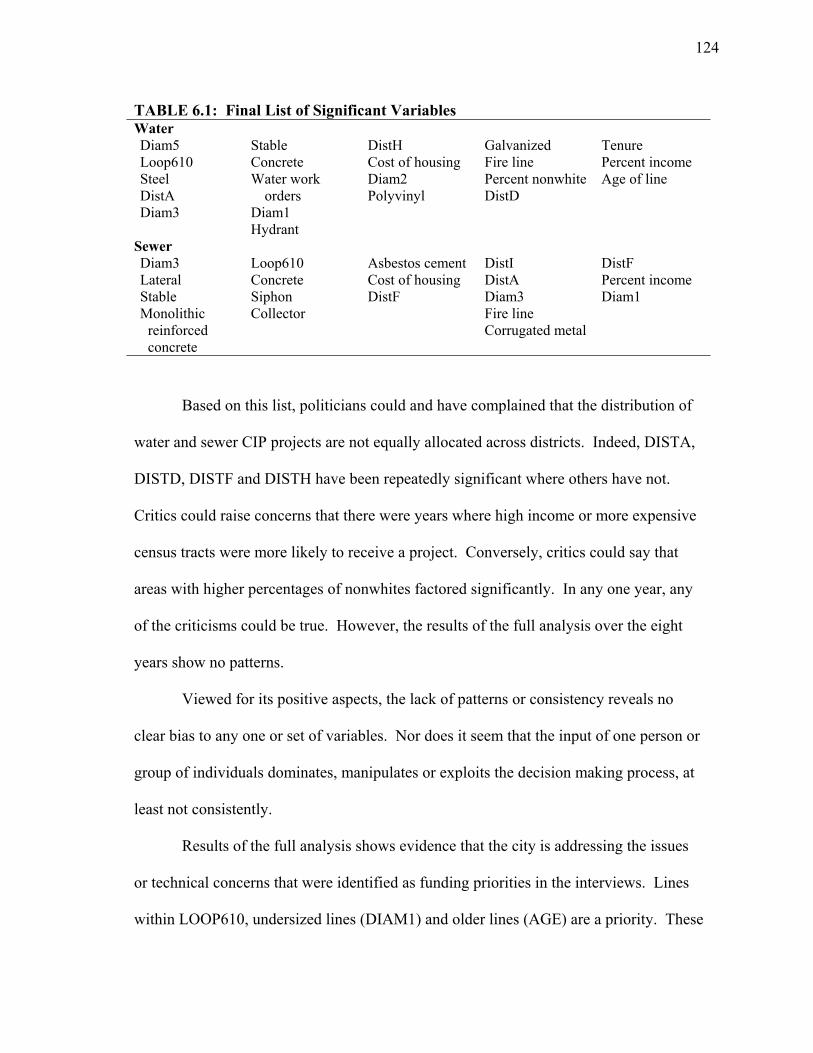
124

TABLE 6.1: Final List of Significant Variables Water Diam5 Loop610 Steel DistA Diam3

Stable Concrete Water work

orders Diam1 Hydrant

DistH Cost of housing Diam2 Polyvinyl

Galvanized Fire line Percent nonwhite DistD

Tenure Percent income Age of line

Sewer Diam3 Lateral Stable Monolithic

reinforced concrete

Loop610 Concrete Siphon Collector

Asbestos cement Cost of housing DistF

DistI DistA Diam3 Fire line Corrugated metal

DistF Percent income Diam1

Based on this list, politicians could and have complained that the distribution of

water and sewer CIP projects are not equally allocated across districts. Indeed, DISTA,

DISTD, DISTF and DISTH have been repeatedly significant where others have not.

Critics could raise concerns that there were years where high income or more expensive

census tracts were more likely to receive a project. Conversely, critics could say that

areas with higher percentages of nonwhites factored significantly. In any one year, any

of the criticisms could be true. However, the results of the full analysis over the eight

years show no patterns.

Viewed for its positive aspects, the lack of patterns or consistency reveals no

clear bias to any one or set of variables. Nor does it seem that the input of one person or

group of individuals dominates, manipulates or exploits the decision making process, at

least not consistently.

Results of the full analysis shows evidence that the city is addressing the issues

or technical concerns that were identified as funding priorities in the interviews. Lines

within LOOP610, undersized lines (DIAM1) and older lines (AGE) are a priority. These

125

variables have been significant throughout the study period. But again, this is not the

case in every year. And, because the results for water and sewer were not the same, we

could make the assumptions that for the different systems there are different needs at

different times and, most importantly, different individuals forming the prioritized lists.

Most importantly, keep in mind that the multivariate results reflect decisions

made solely for the allocation of underground lines. Decision makers are allocating

funds for the entire system. That includes pumps, lines, treatment facilities, etc. Each

player at the table is advocating for his/her section. Therefore, the decision makers are

operating within a larger context, the details of which were not shared with this

researcher. One issue is a funding cap. We do not know what potential projects were

denied due to limited funding. We also don’t know what role federal or state regulations

played in determining project selection.

So, in sum, we know that work orders have been significant. We know what

other variables are factored into the decision making process. Prior to determining the

value, if any, of that list, critics must understand that the study of the decision making

process is not an exact science. The results are based on information that is available

and the methods used.

Summary of Model Fit Findings

The results of the model fit analysis help tie the results of multivariate analysis to

the literature on citizen contacts and urban service delivery.

126

The bivariate and simple model tested the direct relationship between citizen

contacts, i.e., work orders and project allocation or government response. When the

simple model was compared to the theory models, the –2 Log Likelihood indicated that

work orders are not the sole factor in the decision making process. If that were the case,

the results of the simple and full model for water and sewer would have been the same

i.e. work orders would have been the only significant variable. Therefore, government

response to citizen contacts cannot be accurately evaluated with a single variable model.

One must consider the bigger picture or context of those contacts. Part of evaluating the

strength of the urban service delivery models lies in the variables selected.

The class bias model tested four variables; percent ownership, median household

income, percent non-white and average housing cost. Implementing the suggestions of

Bolotin and Cingranelli (1983) and Mladenka (1989), I looked for distributional patterns

over time. Still, the final results showed little support for this theory. Only in 1998 was

the class bias the dominate model. In most years, the addition of the class bias variables

resulted in a slight improvement over the simple model. In a few years there was no

improvement.

The decision rules literature suggested that the internal rules and/or professional

criteria be more thoroughly explored (Jones et al., 1978; Sanger, 1982) . Following

those suggestions, the interviews with PW&E suggested five variables that were part of

the agencies internal rules: age of the line, line location, diameter, type and material.

Among the model fit analysis, the decision rules water model was the better fit in 62

percent of the years. That was not the case for sewer. In no year did the decision rules

model prove to be a better fit. However, the value difference between the decision rules

127

and full model was small. The decision rules model proved to be a subset of the full

model.

Consider the conclusions of Mladenka (1978) and Sanger (1982); that the

Decision Rules theory really only explained the decision making process, not the

resulting distributional patterns. Given this we should expect the variables representing

the decision rules model to be predominate, and they are.

Research on the Political Influence model suggested a variety of factors to

consider. Many of the concepts were difficult to quantify or, the information was not

available or, it was not explicitly used by those involved in the decision making process.

Following Meier’s (1991) and Rowan and Tunyavong’s (1994) suggestion of

studying one city over time resulted in no support for the Political Influence theory.

Not only was it never the dominate model, but in several years, 1993 and 1996

for water in 1992, 1993, 1995 and 1996 for sewer, the addition of the political variables

was not a model improvement over the intercept only model.

The results of the full model tells us that each of the models, to varying degrees,

contributes something to the selection of CIP projects. Though that contribution is not

the same each year. What we have learned from the full model is the importance of

long-term study. The conclusions reached by many of the urban service delivery studies

captured a picture in time. If we look at the water study, say in 1998, the results support

the Class Bias theory, in other years, the results would support the Decision Rules. The

same range of results can be said, although to a lesser degree, for sewer.

128

Implications

Implications for City of Houston

The city is doing an admirable job of providing the community with information.

It has created a multitude of avenues where the public can request information, submit

complaints or make suggestions. However, problems continue to plague PW&E.

During the writing of this dissertation, the Houston’s PW&E was restructured at least

once. In late January of 2002, the department head resigned and the department was

harshly criticized as the department of “burst pipes and mangled streets” (Graves, 2002).

It would help the situation if the public had a better understanding of how the

infrastructure decision making process works, what factors are considered and what are

the goals that the process is designed to achieve. That goal(s) may need to be shared

among all the decision makers. At this time, different groups are operating attempting to

satisfy many objectives.

City planners should be included in the decision making process. The decisions

made have distributional consequences/effects. Engineers involved in the process

acknowledge the need for a planner’s knowledge at the decision making table. While

engineers look at systems issues, no one within their department is looking at the current

or future, demographic effects or trends. To that end, it would be helpful if the decision

makers determined if their goal or objective was process or effect driven, i.e. equitable

process or equitable outcome. It is possible these goals will be contradictory. This will

make it somewhat easier to measure the results and defend the decisions made. Also,

now that the city has an updated GIS system, it should be possible to conduct an impact

129

analysis and graphically depict the location of proposed projects prior to the final

decision such that all parties are aware of potential impacts and can discuss or modify

them.

Finally, to the extent possible, the city should complete the inventory of the water

and sewer system. A systematic method of updating the system inventory and condition

assessment should also be considered. The method should include a way of retaining

historical information of replaced lines. Historical information will prove useful in

analyzing line life spans, etc.

Implications for Future Research

During the data collection and writing of this dissertation, several issues

presented themselves as needing further research.

Methodology. For this research, the decision making process was tested using a

logistic regression. Other, non-statistical methods can be applied. These methods may

be able to capture nuances not incorporated in a statistical model. A tree structured non-

parametric data analysis such as a classification and regression tree (CART) is designed

so that statistical concerns such as normality are not an issue. The results of various

methodologies may be different. A comparison of results may prove interesting.

Cost, regulatory factors, and environmental considerations were not incorporated

into the model. If this information could be captured and manipulated, the results may

be different. In addition, all elements of a given system, be it water or sewer should be

evaluated together since they all compete for the same funds under the same funding

cap.

130

There is a wealth of information contained in the bivariate analyses. Future

research may evaluate these relationships to their fullest extent and discuss possible

implications on citizen contacts or on the priorities/criteria to be followed when selecting

capital improvement projects.

Contributions to Literature. There is a growing body of literature on the output

of urban service distribution. Issues of equity or unpatterned inequalities still exists.

This study focused on the decision making process of urban services. It did not evaluate

the distributional effects or patterns of project allocation. Mladenka and Hill (1978)

argue that the decision rules employed in the decision making process were not

necessarily neutral in their effects. The effects may be random or unanticipated

(Antunes & Plumlee, 1977). A future study may incorporate the use of GIS to spatially

analyze the distributional patterns over time and in consideration with population shifts,

tenure, etc. The objective would be to determine if biases exist in the CIP program and

if so, what are they.

When evaluating the distributional patterns, it will be important to incorporate

the lessons learned in the literature review presented in Chapter II.

Evaluate distributional patterns over time to capture political and

socioeconomic changes.

Distinguish between capital and programs.

Distinguish between emergency, short-term or long-term

programs/responses.

Use a variety of indicators.

131

The data that is maintained by Houston’s Customer Response Center is

extensive. The data set contains call location, time and date of call, reason for call,

department referred to, date and time of department response, etc. That information, if

aggregated or otherwise modified (to provide anonymity) and studied would contribute

to the literature on citizen-initiated contacts and government’s immediate response. This

information is available not just for sewer and water but for all city services to which the

Customer Response Center provides support.

Implications for Planning

In 1986, Arthur Nelson wrote an article entitled Teaching planners about

infrastructure: a call to civil engineers. In that article he stated that, “more than 40

percent of the more than 20,000 planners in the United States influence the manner in

which water, sewer, drainage, streets, and other kinds of physical infrastructure are

planned and used.” His concern was to what extent planners are educated about

infrastructure. Transportation planning is a specialization within planning but it does not

cover the other infrastructure elements. At the time of his study, only 10 percent of the

universities that offered planning included infrastructure as a course in their curriculum

(either offered within their department or cross-listed with engineering). The extent to

which that number has increased or decreased and the benefits of such an infrastructure

course in the planning curriculum is a topic for future research.

There are many opportunities for planners to collaborate with engineers, public

administrators, etc. It is clear that each discipline brings valuable information to the

132

discussion. Between planners and engineers specifically, a better relationship could be

fostered if planners were involved in more steps of the CIP progress.

Proactive vs reactive. This is a long-time discussion among the planning

profession. The benefits and disadvantages to both as well as when either action would

be appropriate is a point for discussion.

133

REFERENCES

Abney, G. & Lauth, T. (1982). A comparative analysis of distributional and

enforcement decisions in cities. The Journal of Politics, 44(1), 193-200.

American Society of Planning Officials. (1951). Capital improvement programming -

some consideration, Planning Advisory Service Information Report No. 23.

Chicago, IL: Author.

Antunes, G. & Plumlee, J. (1977). The distribution of an urban public service:

Ethnicity, socioeconomic status, and bureaucracy as determinants of the quality

of neighborhood streets. Urban Affairs Quarterly, 12(3), 313-32.

Arnstein, S.R. (1969). A ladder of citizen participation. Journal of the American

Institute of Planners, 36, 216-224.

Baer, W.C. (1985). Just what is an urban service anyway? Journal of Politics, 47(3),

881-98.

Balla, Steven J. (2000). Political and organizational determinants of bureaucratic

responsiveness. American Politics Quarterly, 28(2), 163-93.

Barrett, K & Greene, R. (2000, April). Grading the cities: A management report card.

Governing. Available: http://governing.com.

Bimber, B. (1999). The Internet and citizen communication with government: Does the

medium matter? Political Communication, 16(4), 409-28.

Bolotin, F.N. & Cingranelli, D.L. (1983). Equity and urban policy: The underclass

hypothesis revisited. Journal of Politics, 45(1), 209-19.

134

Bowyer, R.A. (1993). Capital improvements: Linking budgeting and planning,

Planning Advisory Service Report No. 442. Chicago, IL: American Planning

Association.

Boyle, J. & Jacobs, D. (1982). The intra city distribution of services: A multivariate

analysis. The American Political Science Review, 76(2), 371-79.

Brown, S.D. (1982). The explanation of particularized contacting: A comparison of

models. Urban Affairs Quarterly, 18(2), 217-34.

Cain, L.P. (1997). Historical perspective on infrastructure and U.S. economic

development. Regional Science & Urban Economics, 27(2), 117-38.

Cingranelli, D.L. (1981). Race, politics and elites: Testing alternative models of

municipal services distribution. American Journal of Political Science, 25(4),

664-92.

Coulter, P.B. (1988). Political voice: Citizen demand for urban public services.

Tuscaloosa, AL: The University of Alabama Press.

Coulter, P.B. (1992). There’s a madness in the method: Redefining citizen contacting

of government officials. Urban Affairs Quarterly, 28(2), 297-316.

Creighton, J.L. (1999). Public participation in federal agencies’ decision making in the

1990s. National Civic Review, 88(3), 249-58.

Crihfield, J.B. & McGuire, T.J. (1997). Infrastructure economic development and

public policy. Regional Science and Urban Economics, 27(2), 113-16.

Dawson-Saunders, B. & Trapp, R. (1990). Basic and clinical biostatistics. Norwalk,

CN: Appleton & Lange.

135

Day, T.J. (1998). Sewer infrastructure management: New concepts and tools for your

collector system. Water Engineering and Management, 145(2), 26-29.

Eisinger, P. (1972). The pattern of citizen contacts with urban officials. In H. Hahn

(Ed.), People and politics in urban society (pp. 43-69). Beverly Hills, CA: Sage

Publishing.

Federal Public Works. Infrastructure R&D: A new perspective. (1993). Washington,

DC: Civil Engineering Research Foundation (CERF).

Feiock, R. (1986). The political economy of urban service distribution: A test of the

underclass hypothesis. Journal of Urban Affairs, 8, 31-42.

Garcia, S. (2000, May 14). Let’s create a new approach. Houston Chronicle, p. 1A.

Goodwin, S.R. & Peterson, G.E. (1983). Infrastructure inventory and condition

assessment: Tools for improving capital planning and budgeting. Washington

DC: The Urban Institute Press.

Goodwin, S.R. & Peterson, G.E. (1984). Guide to assessing capital stock condition.

Washington, DC: The Urban Institute Press.

Graves, R. (2002, January 22). Brown replaces director of public works. Houston

Chronicle, p. 1A.

Greene, K. (1982). Service representation and municipal administrators’ receptivity to

citizen contacts. In R.C. Rich (Ed.), Analyzing urban-service distributions (pp.

61-78). Lexington, MA: Lexington Books.

Grigg, N.S. (1986). Urban water infrastructure: Planning, management and

operations. New York: John Wiley & Sons.

136

Grigg, N.S. (1988). Infrastructure engineering and management. New York: John

Wiley & Sons.

Grigg, N.S. (1994). Infrastructure: A more comprehensive policy is needed. Journal of

Professional Issues in Engineering Education and Practice, 128(2), 183-92.

Habibian, A. (1994). Research needs for water distribution system rehabilitation.

Water Engineering and Management, 141(8), 25-27.

Hatcher, L. & Stepanski, E. (1994). A step-by-step approach to using the SAS system

for univariate and multivariate statistics. Cary, NC: SAS Institute.

Haughwout, A.T. (1995). Central city infrastructure investment and suburban house

values. Regional Science and Urban Economics, 27, 199-215.

Healey, J. (1984). Statistics: A tool for social research. Belmont, CA: Wadsworth

Publishing Company.

Hero, R.E. (1986). Explaining citizen-initiated contacting of government officials:

Socioeconomic status, perceived need or something else? Social Science

Quarterly, 67, 626-35.

Hirlinger, M.W. (1992). Citizen-initiated contacting of local government official: A

mulitvariate explanation. Journal of Politics, 54(2), 553-64.

Hosemer, D. & Lemeshow, S. (2000). Applied logistic regression, 2nd ed. New York:

John Wiley & Sons.

Jacob, H. (1972). Contact with government agencies: A preliminary analysis of the

distribution of government services. Midwest Journal of Political Science, 16(1),

123-46.

137

Jones, B. (1978). Distributional considerations in models of government service

provision. Urban Affairs Quarterly, 12(3), 291-312.

Jones, B.D. (1980). Service delivery in the city: Citizen demand and bureaucratic

rules. New York: Longman, Inc.

Jones, B.D. (1981). Party and bureaucracy: The influence of intermediary groups on

urban public services delivery. American Political Science Review, 75, 688-700.

Jones, B.D., Greenberg, S., Kaufman, C. & Drew, J. (1977). Bureaucratic response to

citizen-initiated contacts: Environmental enforcement in Detroit. The American

Political Science Review, 71, 148-65.

Jones, B.D., Greenberg, S., Kaufman, C.& Drew, J. (1978). Service delivery rules and

the distribution of local government services: Three Detroit bureaucracies.

Journal of Politics, 40(2), 332-68.

King, C.S., Feltey, K.M.& Susel, B.O. (1998). The question of participation: Toward

authentic public participation in public administration. Public Administration

Review, 58(4), 317-26.

Koehn, E., Broz, J., Fisher, J. & McKinney, J. (1985). Estimating rural and urban

infrastructure needs. Journal of Professional Issues in Engineering, 111, 48-56.

Koehler, D.H. & Wrightson, M.T. (1987). Inequality in the delivery of urban services:

A reconsideration of the Chicago parks. Journal of Politics, 49(1), 80-99.

Lando, T. (1999). Public participation in local government: Points of view. National

Civic Review, 88(2), 109-22.

Lee, S.J. (1994). Policy type bureaucracy and urban policies: Integrating models of

urban service distribution. Policy Studies Journal, 22(1), 87-108.

138

Lehnen, R.G. (1976). American institutions, political opinion and public policy.

Hinsdale, IL: Dryden Press.

Levy, F., Meltsner, A. Wildavsky, A. (1974). Urban outcomes. Berkeley, CA:

University of California Press.

Lineberry, R. (1975). Equality, public policy and public services: The underclass

hypothesis and the limits to equality. Policy and Politics, 4, 67-84.

Lytton, R.L. (1991). Infrastructure: Back to Cadbury or on to Camelot? Unpublished

doctoral dissertation, Texas A&M University, College Station, TX.

Meier, K.J., Stewart, J. & England, R. (1991). The politics of bureaucratic discretion:

Educational access as an urban service. American Journal of Political Science,

35(1), 155-77.

Mladenka, K.R. (1977). Citizen demand and bureaucratic response: Direct dialing

democracy in a major American city. Urban Affairs Quarterly, 12(3), 273-91.

Mladenka, K.R. (1978). Organizational rules, service equality and distributional

decisions in urban politics. Social Science Quarterly, 59(1), 192-201.

Mladenka, K.R. (1980). The urban bureaucracy and the Chicago political machine:

Who gets what and the limits to political control. American Political Science

Review, 74(4), 991-98.

Mladenka, K.R. (1981). Citizen demands and urban services: The distribution of

bureaucratic response in Chicago and Houston. American Journal of Political

Science, 25(4), 693-714.

Mladenka, K.R. (1989). The distribution of an urban public service: The changing role

of race and politics. Urban Affairs Quarterly, 24(4), 556-83.

139

Mladenka, K.R. & Hill, K.Q. (1978). The distribution of urban police services. Journal

of Politics, 40(1), 112-33.

Nardulli, P.F. & Stonecash, J.M. (1982). Toward a theoretical framework for analyzing

urban service distributions. In R.C. Rich (Ed.), Analyzing urban service

distribution (pp. 45-59). Lexington, MA: Lexington Books.

Nelson, A.C. (1986). Teaching planners about infrastructure: A call to civil engineers.

Journal of Urban Planning and Development, 113(2), 67-76.

Nivola, P. (1978). Distributing a municipal service: A case study of housing

inspection. Journal of Politics, 40(1), 59-81.

Peterson, S.A. (1986). Close encounters of the bureaucratic kind: Older Americans and

bureaucracy. American Journal of Political Science, 30(2), 347-356.

Peterson, S.A. (1988). Sources of citizens’ bureaucratic contacts: A multivariate

analysis. Administration & Society, 20(2), 152-65.

Potter, H. & Norville, H. (1983). Citizens’ participation and effectiveness in

environmental issues. In G.A. Daneke (Ed.), Public involvement and social

impact assessment (pp. 35-44). Boulder, CO: Westview Press.

Rittel, H. & Webber, M. (1973). Dilemmas in a general theory of planning. Policy

Sciences, 4, 155-69.

Rosener, J.B. (1978). Citizen participation: Can we measure its effectiveness? Public

Sciences, 4, 155-69.

Rowan, M. & Tunyavong, I. (1994). Patterned inequality? Reexamining the role of

distributive politics in urban service delivery. Urban Affairs Quarterly, 29(4),

509-34.

140

Sanders, H.T. (1973). What infrastructure crisis? Public Interest, 110, 3-18.

Sanger, M. (1982). Academic models and public policy: The distribution of city

services in New York. In R.C. Rich (Ed.), The politics of urban public services

(pp. 37-51). Lexington, MA: Lexington Books.

Schwartz, M. (2000, April 19). Public works department head quits. Houston

Chronicle, p. 1A.

Seely, B.E. (1993). A republic bound together. The Wilson Quarterly, 17, 18-39.

Sharp, E. (1982). Citizen-initiated contacting of local government officials and

socioeconomic status: Determining the relationship and accounting for it.

American Political Science Review, 76(1), 109-15.

Sharp, E. (1984). Citizen demand-making in the urban context. American Journal of

Political Science, 28(4), 654-70.

Sharp, E. (1986). Citizen demand making in the urban context. Birmingham, AL:

University of Alabama Press.

Snodgrass, R., Kiengle, W. & Labriola, A. (1996). Taking infrastructure management

systems into the next century. Public Works, 27, 7-13.

So, F. (1962). Capital improvement programming. Chicago, IL: American Society of

Planning Officials, Planning Advisory Service Information Report No. 151.

So, F.S., Stollman, I.B., Beal, F. & Arnold, D. (1979). The practice of local government

planning, 3rd ed. Washington, DC: International City Management Association.

Talen, E. (1997). The social equity of urban service distribution: An exploration of

park access in Pueblo, Colorado and Macon, Georgia. Urban Geography, 18(6),

521-541.

141

Thomas, J.C. (1982). Citizen-initiated contacts with government agencies: A test of

three theories. American Journal of Political Science, 26(3), 504-22.

Thomas, J.C. & Melkers, J. (1999). Explaining citizen-initiated contacts with municipal

bureaucrats. Urban Affairs Review, 43(5), 667-90.

Thornton, W.J. & Ulrich, H.D. (1993). Infrastructure-management-system analysis.

Journal of Urban Planning and Development, 119(1), 39-47.

Traut, C. & Emmert, C. (1993). Citizen-initiated contacting: A multivariate analysis.

American Politics Quarterly, 21(2), 239-53.

Vedlitz, A. & Dyer, J.A. (1984). Bureaucratic response to citizen contacts:

Neighborhood demands and administrative reaction in Dallas. Journal of

Politics, 45, 1207-16.

Vedlitz, A., Dyer, J.A. & Durand, R. (1980). Citizen contacts with local governments:

A comparative view. American Journal of Political Science, 24(1), 50-67.

Vedlitz, A & Veblen, E. (1980). Voting and contacting two forms of political

participation in a suburban community. Urban Affairs Quarterly, 16, 31-48.

Verba, S. & Nie, N. (1972). Participation in America: Political and democracy and

social equity. New York: Harper and Row.

Viteritti, J. (1982). Bureaucratic environments, efficiency, and equity in urban-service-

delivery systems. In R. Rich (Ed.), The politics of urban public services (pp. 53-

68). Lexington, MA: Lexington Books.

Zuckerman, A.S. & West, D.M. (1985). The political basis of citizen contacting: A

cross-national analysis. American Political Science Review, 79(1), 117-31.

142

APPENDIX A

DESCRIPTIVE STATISTICS

N Min Max Mean Median Std. Dev. Freq

Cum Freq

Water work orders

Water work orders 1992 375 1 4 2.53 2 1.136 1 91 91

2 98 189

3 82 271

4 104 375

Water work orders 1993 375 1 4 2.533 2 1.058 1 75 75

2 113 188

3 99 287

4 88 375

Water work orders 1994 375 1 4 2.568 2 1.069 1 71 71

2 117 188

3 90 278

4 97 375

Water work orders 1995 375 1 4 2.541 2 1.122 1 85 85

2 106 191

3 80 271

4 104 375

Water work orders 1996 375 1 4 2.581 2 1.134 1 82 82

2 106 188

3 74 262

4 113 375

Water work orders 1997 375 1 4 2.573 2 1.123 1 81 81

2 107 188

3 78 266

4 109 375

Water work orders 1998 375 1 4 2.536 2 1.176 1 99 99

2 89 188

3 74 262

4 113 375

Water work orders 1999 375 1 4 2.562 2 1.128 1 84 84

2 104 188

3 79 267

4 108 375

143

Sewer work orders

Sewer work orders 1992 375 1 4 2.528 2 1.203 1 103 103

2 92 195

3 59 254

4 121 375

Sewer work orders 1993 375 1 4 2.5466 2 1.18 1 97 97

2 93 190

3 68 258

4 117 375

Sewer work orders 1994 375 1 4 2.608 2 1.136 1 78 78

2 110 188

3 68 256

4 119 375

Sewer work orders 1995 375 1 4 2.5973 2 1.133 1 79 79

2 109 188

3 71 259

4 116 375

Sewer work orders 1996 375 1 4 2.549 2 1.1572 1 92 92

2 97 189

3 74 263

4 112 375

Sewer work orders 1997 375 1 4 2.525 2 1.169 1 99 99

2 90 189

3 76 265

4 110 375

Sewer work orders 1998 375 1 4 2.56 2 1.204 1 101 101

2 87 188

3 63 251

4 124 375

Sewer work orders 1999 375 1 4 2.56 2 1.195 1 99 99

2 89 188

3 65 253

4 122 375

144

Demographic Model

N Min Max Mean Median Std. Dev. Freq Cum Freq

Percent nonwhite 375 1 4 2.525 2 1.174 1 97 97

2 98 195

3 66 261

4 114 375

Median hh income 375 0 3 1.824 2 0.5813 1 102 102

2 237 339

3 36 375

Percent ownership 375 0 100 45.0533 46 22.971904

Median Hsng Cst (index of below) 375 0 10.5 5.5946 5.5 1.7481001

Median house value 375 0 1060300 76019.6 54400 86010.97

Median rent 375 0 1001 427.978 406 151.94177

Objective Model

Water

DIAM1 >= 2.5 375 0 1 0.4986 0 0.5006 0 188 188

1 187 375

DIAM2 2.5 <> 6 375 0 1 0.4986 0 0.5006 0 188 188

1 187 375

DIAM3 8 <> 12 375 0 1 0.4986 0 0.5006 0 188 188

1 187 375

DIAM4 12 <> 24 375 0 1 0.488 0 0.5005 0 192 182

1 183 375

DIAM5 > 24 375 0 1 0.4026 0 0.49109 0 224 224

1 151 375

T_MAIN main line 375 0 1 0.496 0 0.5006 0 189 189

1 186 375

T_WCL well collection line 375 0 1 0.1386 0 0.34606 0 323 323

1 52 375

T_COLL collector 375 0 1 0.3733 0 0.18983 0 361 361

1 14 375

T_HYDL hydrant lead 375 0 1 0.4986 0 0.50066 0 188 188

1 187 375

T_FIRE fire line 375 0 1 0.4533 0 0.498482 0 205 205

1 170 375

T_CASE casing 375 0 1 0.3733 0 0.4843357 0 235 235

1 140 375

T_TRANS transmission line 375 0 1 0.04 0 0.196221 0 360 360

1 15 375

145

M_AC asbestos 375 0 1 0.4986 0 0.5006 0 188 188

1 187 375

M_CI cast iron 375 0 1 0.4986 0 0.5006 0 188 188

1 187 375

M_CONC concrete 375 0 1 0.08266 0 0.2757 0 344 344

1 31 375

M_COP copper 375 0 1 0.2266 0 0.4192 0 290 290

1 85 375

M_DI ductile iron 375 0 1 0.296 0 0.4571 0 264 264

1 111 375

M_GALV galvanized iron 375 0 1 0.3786 0 0.4857 0 233 233

1 142 375

M_PCPE pcpe 375 0 1 0.032 0 0.1762 0 363 363

1 12 375

M_PCPL pcpl 375 0 1 0.0133 0 0.1148 0 370 370

1 5 375

MAT78 pcpe/pcpl 375 0 1 0.0426 0 0.2023 0 359 359

1 16 375

M_PVC polyvinyl 375 0 1 0.5006 0 0.5006 0 190 190

1 185 185

M_SRC steel cylinder 375 0 1 0.2674 0 0.2674 0 346 346

1 29 375

M_STL steel 375 0 1 0.3542 0 0.3542 0 55 55

1 320 375

AGE median age of housing 375 0 90 68.402 70 14.1362

SERV repair date 375 0 90 24.7733 0 36.2977

Loop610 375 0 1 0.304 0 0.4605 0 261 261

1 114 375

Sewer

T CASE casing 375 0 1 0.1626 0 0.3695 0 314 314

1 61 375

T COLL collector 375 0 1 0.4986 0 0.5006 0 188 188

1 187 375

T FM force main 375 0 1 0.4133 0 0.493 0 220 220

1 155 375

T LATL lateral 375 0 1 0.4266 0 0.4952 0 215 215

1 160 375

T OF overflow 375 0 1 0.2986 0 0.4582 0 262 262

1 112 375

T SIPH siphon 375 0 1 0.1653 0 0.3719 0 313 313

1 62 375

146

T SLDG sludge 375 0 1 0.0746 0 0.2632 0 347 347

1 28 375

T STUB sub 375 0 1 0.4986 0 0.5006 0 188 188

1 187 375

M ABS acrylonitrile buadiniene styrene 375 0 1 0.4586 0 0.4989 0 203 203

1 172 375

M CGMP corrugated metal pipe 375 0 1 0.0933 0 0.2912 0 340 340

1 35 375

M CI cast iron 375 0 1 0.48 0 0.5002 0 196 196

1 179 375

M CLAY clay 375 0 1 0.24 0 0.4276 0 285 385

1 90 375

M CONC concrete 375 0 1 0.496 0 0.5006 0 189 189

1 186 375

M DI ductile iron 375 0 1 0.4746 0 0.5002 0 197 197

1 178 375

M ESP extra strength concrete pipe 375 0 1 0.496 0 0.5006 0 189 189

1 186 375

M MRC monlithic reinforced concrete 375 0 1 0.416 0 0.4935 0 219 219

1 156 375

M PVC polyvinyl chloride 375 0 1 0.4933 0 0.5006 0 190 190

1 185 375

M RCP reinforced concrete pipe 375 0 1 0.4933 0 0.5006 0 190 190

1 185 375

M STL steel 375 0 1 0.1786 0 0.3835 0 308 308

1 67 375

DIAM1 0 < > 4 375 0 1 0.336 0 0.4729 0 249 249

1 126 375

DIAM2 6 < > 8 375 0 1 0.496 0 0.5006 0 189 189

1 186 375

DIAM3 10 < > 20 375 0 1 0.4933 0 0.5006 0 190 190

1 185 375

DIAM4 > 20 375 0 1 0.4853 0 0.5004 0 193 193

147

Political Model

N Min Max Mean Median Std. Dev. Freq

Cum Freq

VOTE92 64 1 4 2.5937 2.5 1.178 1 15 23.44

2 17 50

3 11 67.19

4 21 100

VOTE93 64 1 4 2.5937 2.5 1.1229 1 13 20.31

2 19 50

3 13 70

4 19 100

VOTE94 64 1 4 2.5312 205 1.0978 1 14 21.88

2 18 50

3 16 75

4 16 100

VOTE95 64 1 4 2.5312 2.5 1.0978 1 14 21.88

2 18 50

3 16 75

4 16 100

VOTE97 64 1 4 2.6406 2.5 1.0445 1 12 18.75

2 20 50

3 16 75

4 16 100

VOTE98 64 1 4 2.6262 2.5 1.0573 1 9 14.06

2 32 50

3 45 71

4 64 100

VOTE99 64 1 4 2.625 2.5 1.091 1 11 17.19

2 32 50

3 45 70.31

4 64 100

TEN92 375 2 6 4.986 6 1.742

TEN93 375 1 6 2.04 1 1.614

TEN94 375 2 6 3.04 2 1.617

TEN95 375 1 5 2.578 3 1.284

TNE96 375 2 6 3.578 4 1.284

TEN97 375 1 5 3.858 5 1.379

TNE98 375 2 6 4.858 6 1.379

TEN99 375 1 5 2.594 1 1.84

ELYR Value yes or no 375

148

STABLE Value yes or no 375 0 2 0.0666 0 0.3406 0 360 360

1 5 365

2 10 375

ACTIVE93 64 0 1 0.4843 0 0.5037 0 33 51.56

1 64 100

ACTIVE94 64 0 1 0.4843 0 0.5037 0 33 51.56

1 64 100

ACTIVE95 64 0 1 0.4843 0 0.5037 0 33 51.56

1 64 100

ACTIVE96 64 0 1 0.4843 0 0.5037 0 33 51.56

1 64 100

ACTIVE97 64 0 1 0.4843 0 0.5037 0 33 51.56

1 64 100

ACTIVE98 64 0 1 0.4843 0 0.5037 0 33 51.56

1 64 100

ACTIVE99 64 0 1 0.4843 0 0.5037 0 33 51.56

DISTA 43 0 1 0.1146 0 0.319 0 332 332

1 43 375

DISTB 47 0 1 0.1253 0 0.3315 0 328 328

1 47 375

DISTC 40 0 1 0.1066 0 0.3091 0 335 335

1 40 375

DISTD 52 0 1 0.1386 0 0.346 0 323 323

1 52 375

DISTE 36 0 1 0.096 0 0.2949 0 339 339

1 36 375

DISTF 23 0 1 0.0613 0 0.2402 0 352 352

1 23 375

DISTG 39 0 1 0.104 0 0.3056 0 336 336

1 39 375

DISTH 55 0 1 0.1466 0 0.3542 0 320 320

1 55 375

DISTI 40 0 1 0.1066 0 0.3091 0 335 335

1 40 375

149

Dependent Variable

N Min Max Mean Median Std. Dev. Freq Cum Freq

WCIP92 375 0 1 0.18933 0 0.3922966 0 304 304

1 375 375

WCIP93 375 0 1 0.09333 0 0.2912876 0 340 340

1 375 375

WCIP94 375 0 1 0.13067 0 0.3374857 0 326 326

1 49 375

WCIP95 375 0 1 0.144 0 0.3515588 0 321 321

1 54 375

WCIP96 375 0 1 0.08533 0 0.2797503 0 343 343

1 32 375

WCIP97 375 0 1 0.14933 0 0.3568929 0 319 319

1 56 375

WCIP98 375 0 1 0.08 0 0.2716556 0 345 345

1 30 375

WCIP99 375 0 1 0.072 0 0.2588333 0 348 348

1 27 375

SCIP92 375 0 1 0.12 0 0.3253957 1 330 330

2 45 375

SCIP93 375 0 1 0.0933 0 0.2912876 1 340 340

2 35 375

SCIP94 375 0 1 0.06133 0 0.2402613 1 352 352

2 23 375

SCIP95 375 0 1 0.07466 0 0.2632039 1 347 347

2 28 375

SCIP96 375 0 1 0.07467 0 0.2632039 1 347 347

2 28 375

SCIP97 375 0 1 0.13333 0 0.3403888 1 325 325

2 50 375

SCIP98 375 0 1 0.06667 0 0.2497771 1 350 352

2 25 375

SCIP99 375 0 1 0.06667 0 0.24977771 1 350 350

2 25 375

150

APPENDIX B: COMPLETE CLASS BIAS MULTIVARIATE ANALYSIS

Estimate (p-value) Odds Ratio Confidence Intervals Water 1992 WWO .7063 .0001 2.026 (1550 2.650) COST .2086 .8167 1.029 (.808 1.311) MIN .1715 .2976 1.187 (.860 1.639) INC .5027 .2082 1.653 (.756 3.616) OWN -.0041 .5254 .996 (.983 1.009) -2 Log Likelihood Likelihood Ratio Score intercept only 363.941 Chi-square 31.7123 Chi-square 30.1832 with covariates 332.224 p-value <.0001 p-value <.0001

Estimate (p-value) Odds Ratio Confidence Intervals Water 1993 WWO .4271 .0152 1.533 (1.086 2.164) MIN .3565 .0958 1.428 (.939 2.173) COST -.2192 .1896 .803 (.579 1.114) INC .3648 .4518 1.440 (.557 3.725) OWN .0036 .6812 1.004 (.987 1.021) -2 Log Likelihood Likelihood Ratio Score intercept only 232.637 Chi-square 12.5110 Chi-square 12.2843 with covariates 220.126 p-value .0019 p-value .0030

Estimate (p-value) Odds Ratio Confidence Intervals Water 1994 MIN .4961 .0093 1.642 (1.130 2.387) WWO .1922 .1959 1.212 (.906 1.622) COST -.0609 .6755 .941 (.707 1.252) OWN .0057 .4453 1.006 (.991 1.021) INC .1033 .8034 1.109 (.492 2.500) -2 Log Likelihood Likelihood Ratio Score intercept only 290.739 Chi-square 12.0683 Chi-square 11.7749 with covariates 278.671 p-value .0005 p-value .0006

Estimate (p-value) Odds Ratio Confidence Intervals Water 1995 WWO .2430 .0035 1.275 (.976 1.667) COST -.0091 .9450 .991 (.764 1.285) MIN .2227 .2055 1.249 (.885 1.764) INC .1695 .6755 1.185 (.536 2.620) OWN .0030 .6662 1.003 (.989 1.017) -2 Log Likelihood Likelihood Ratio Score intercept only 309.119 Chi-square NA Chi-square NA with covariates NA p-value NA p-value NA

151

Estimate (p-value) Odds Ratio Confidence Intervals Water 1996 WWO .2596 .1411 1.296 (.918 1.832) COST .3693 .0312 1.447 (1.034 2.024) MIN .5693 .0185 1.757 (1.099 2.809) INC .0179 .9725 1.018 (.369 2.811) OWN -.0059 .4866 .994 (.978 1.011) -2 Log Likelihood Likelihood Ratio Score intercept only 218.704 Chi-square 7.3505 Chi-square 6.9248 With covariates 211.354 p-value .2534 p-value .0314

Estimate (p-value) Odds Ratio Confidence Intervals Water 1997 WWO .3285 .0162 1.389 (1.063 1.815) COST .0288 .8223 1.029 (.800 1.324) MIN .0701 .6881 1.073 (.762 1.510) INC .1229 .7631 1.131 (.509 2.514) OWN -.0060 .3750 .994 (.981 1.007 -2 Log Likelihood Likelihood Ratio Score intercept only 316.163 Chi-square 6.0386 Chi-square 5.9567 with covariates 310.125 p-value .0140 p-value .0147

Estimate (p-value) Odds Ratio Confidence Intervals Water 1998 WWO .4548 .0126 1.576 (1.103 2.252) COST 1.6669 .0089 5.296 (1.520 18.448) MIN .1252 .4851 1.133 (.797 1.611) INC .2592 .2949 1.296 (.798 2.105) OWN -.0151 .1136 .985 (.967 1.004) -2 Log Likelihood Likelihood Ratio Score intercept only 209.077 Chi-square 20.94 Chi-square 19.80 with covariates 188.131 p-value .0001 p-value .0001

Estimate (p-value) Odds Ratio Confidence Intervals Water 1999 WWO .6249 . 0025 1.868 (1.245 2.803) COST -.1610 .3821 .851 (.593 1.221) INC 1.553 .0116 4.726 (1.414 15.794) OWN -.0018 .8513 .998 (.979 1.107) MIN .3636 .1319 1.438 (.896 2.308) -2 Log Likelihood Likelihood Ratio Score intercept only 194.086 Chi-square 15.34 Chi-square 14.48 with covariates 178.745 p-value .0015 p-value .0023

152

Estimate (p-value) Odds Ratio Confidence Intervals Sewer 1992 COST .2170 .1344 1.242 (.395 1.651) SWO .2095 .1300 1.233 (.940 1.617) INC .6720 .1509 1.958 (.783 4.899) MIN .3268 .1015 1.387 (.938 2.050) OWN -.0092 .2262 .991 (.976 1.006) -2 Log Likelihood Likelihood Ratio Score intercept only 275.194 Chi-square 5.5456 Chi-square 5.7051 with covariates 269.48 p-value .0185 p-value .0169

Estimate (p-value) Odds Ratio Confidence Intervals Sewer 1993 MIN .3365 .1113 1.400 (.925 2.118) SWO .1271 .4103 1.387 (.839 1.537) COST -.2165 .1917 .805 (.582 1.115) INC .3274 .4938 1.387 (.543 3.543) OWN .0028 .7441 1.003 (.986 1.020) -2 Log Likelihood Likelihood Ratio Score intercept only 232.637 Chi-square 6.4442 Chi-square 6.3269 with covariates 226.193 p-value .0111 p-value .0119

Estimate (p-value) Odds Ratio Confidence Intervals Sewer 1994 SWO .5069 .0166 1.660 (1.097 2.513) COST .1118 .5820 1.118 (.751 1.665) INC .5125 .3906 .599 (.186 1.930) MIN .3019 .2626 1.352 (.797 2.294) OWN .0051 .6203 1.005 (.985 1.026) -2 Log Likelihood Likelihood Ratio Score intercept only 172.965 Chi-square 5.3656 Chi-square 5.1883 with covariates 167.600 p-value .0205 p-value .0227

Estimate (p-value) Odds Ratio Confidence Intervals Sewer 1995 SWO .2059 .2512 1.229 (.864 1.747) COST -.0145 .9366 .986 (.828 2.095) INC -.0858 .8711 .918 (.326 2.587) MIN .2755 .2445 1.317 (.987 1.025) OWN .0059 .5286 1.006 (.689 1.410) -2 Log Likelihood Likelihood Ratio Score intercept only 199.160 Chi-square NA Chi-square NA with covariates NA p-value NA p-value NA

153

Estimate (p-value) Odds Ratio Confidence Intervals Sewer 1996 SWO .0919 .6057 1.096 (.773 1.554) COST .3886 .0307 1.475 (.037 2.098) INC .0000 .9993 1.000 (.337 2.972) MIN .4476 .0738 1.564 (.958 2.556) OWN -.0113 .2188 .989 (.971 1.007) -2 Log Likelihood Likelihood Ratio Score Intercept only 199.160 Chi-square 5.9996 Chi-square 5.7145 with covariates 193.160 p-value .0498 p-value .0574

Estimate (p-value) Odds Ratio Confidence Intervals Sewer 1997 SWO .4193 .0008 1.521 (1.153 2.006) COST .1292 .3450 1.138 (.870 1.488) INC .2503 .5684 1.248 (.543 3.036) MIN .0718 .7014 1.074 (.744 1.551) OWN -.0051 .4754 .995 (.981 1.009) -2 Log Likelihood Likelihood Ratio Score Intercept only 294.506 Chi-square 9.7463 Chi-square 9.5296 with covariates 284.760 p-value .0018 p-value .0020

Estimate (p-value) Odds Ratio Confidence Intervals Sewer 1998 INC 1.317 .0491 3.732 (1.005 13.858) WWO 3.011 .1052 1.351 (.939 1.945) COST .1674 .3801 1.182 (.814 1.718) MIN .1580 .5502 1.171 (.697 1.967) OWN -.0166 .1034 .984 (.964 1.003) -2 Log Likelihood Likelihood Ratio Score Intercept only 183.698 Chi-square 9.0618 Chi-square 8.9727 with covariates 174.636 p-value .0026 p-value .0027

Estimate (p-value) Odds Ratio Confidence Intervals Sewer 1999 SWO .5775 .0047 1.782 (1.193 .660) COST -.1604 .4138 .852 (.580 1.252) INC 1.474 .0206 4.369 (1.254 15.22) MIN .2887 .2390 1.335 (.825 2.158) OWN -.0002 .9801 1.000 (.980 1.020) -2 Log Likelihood Likelihood Ratio Score Intercept only 183.698 Chi-square 14.92 Chi-square 14.92 with covariates 168.774 p-value .0107 p-value .0150

154

APPENDIX C: BIVARIATE ANALYSIS OF DECISION RULE VARIABLES

Water

T_MAIN T_COLL T_HYDL T_FIRE T_TRANS M_CI M_CONC M_COP M_CI C=14.20

(.0002) C=.0630 (.8017)

C=1.410 (.2350)

C=.2134 (.6441)

C=4.793 (.0286)

M-CONC C=.9686 (.3250)

C=3.418 (.0645)

C=.0412 (.8391)

C=.1574 (.6915)

C=1.310 (.2523)

M_COP C=4.755 (.0292)

C=.0262 (.8715)

C=3.320 (.0684)

C=.1320 (.7163)

C=.2893 (.5907)

M_DI C=16.48 (.0001)

C=.8444 (.3581)

C=17.80 (.0001)

C=5.889 (.0152)

C=.2609 (.6095)

M_GALV C=10.98 (.0009)

C=2.194 (.1385)

C=5.298 (.0213)

C=1.447 (.2289)

C=3.437 (.0637)

M_PC C=4.313 (.0378)

C=4.930 (.0264)

C=1.067 (.3016)

C=1.987 (.1586)

C=21.03 (.0001)

M_PVC C=34.03 (.0001)

C=1.477 (.2242)

C=22.08 (.0001)

C=2.190 (.1389)

C=4.530 (.0333)

M_SRC C=1.954 (.1621)

C=68.02 (.0001)

C=3.079 (.0793)

C=2.239 (.1346)

C=3.822 (.0506)

M_STL C=24.45 (.0001)

C=.2895 (.5906)

C=13.16 (.0003)

C=12.24 (.0005)

C=.0017 (.9672)

DIAM1

C=29.39 (.0001)

C=.6402 (.4236)

C=.2161 (.6420)

C=.3311 (.5650)

C=1.165 (.2804)

C=67.41 (.0001)

C=4.319 (.0377)

C=36.86 (.0001)

DIAM2

C=176.1 (.0001)

C=2.790 (.0948)

C=219.6 (.0001)

C=11.33 (.0008)

C=.2858 (.5929)

C=4.930 (.0264)

C=.8503 (.3565)

C=.3466 (.5560)

DIAM3

C=222.7 (.0001)

C=6.220 (.0126)

C=142.2 (.0001)

C=25.26 (.0001)

C=2.630 (.1043)

C=1.943 (.1633)

C=.0412 (.8391)

C=4.516 (.0336)

DIAM4

C=29.37 (.0001)

C=14.29 (.0002)

C=35.27 (.0001)

C=12.50 (.0004)

C=.4051 (.5245)

C=4.053 (.0441)

C=.0023 (.9617)

C=3.443 (.0635)

DIAM5

C=6.497 (.0108)

C=2.142 (.1433)

C=1.441 (.2299)

C=9.466 (.0021)

C= 8.871 (.0029)

C=7.154 (.0075)

C=10.60 (.0011)

C=.9005 (.3426)

LOOP 610

C=5.511 (.0189)

C=4.9502 (.0261)

C=11.90 (.0001)

C=.9491 (.3299)

C=6.352 (.0117)

C=31.89 (.0001)

C= .0551 (.8143)

C=57.01 (.0001)

AGE

T=.59 (.5542)

T=-.70 (.4866)

T=1.27 (.2048)

T=.39 (.6949)

T=1.05 (.3116)

T=-4.34 (.0001)

T=.23 (.8166)

T=-.38 (.7066)

= Indicates significance at p=<.05

155

M_DI M_GALV M_PC M_PVC M_SRC M_STL DIAM1 DIAM2 DIAM1

C=.1390 (.7093)

C=118.7 (.0001)

C=1.022 (.3119)

C=8.064 (.0045)

C=.3192 (.5721)

C=.5019 (.4787)

DIAM2

C=19.76 (.0001)

C=1.530 (.2161)

C=.2724 (.6017)

C=18.36 (.0001)

C=4.586 (.0322)

C=6.051 (.0139)

C=1.943 (.1633)

DIAM3

C=14.18 (.0002)

C=6.736 (.0094)

C=2.383 (.1226)

C=51.52 (.0001)

C=.9635 (.3263)

C=20.28 (.0001)

C=9.282 (.0023)

C=123.2 (.0001)

DIAM4

C=39.67 (.0001)

C=.4928 (.4827)

C=.3713 (.5423)

C=5.865 (.0154)

C=11.71 (.0006)

C=10.02 (.0015)

C=.0236 (.8778)

C=26.13 (.0001)

DIAM5

C=.9856 (.3208)

C=.6881 (.4068)

C=19.87 (.0001)

C=.8955 (.3440)

C=13.50 (.0002)

C=2.346 (.1256)

C=5.078 (.0242)

C=.6076 (.4357)

LOOP 610

C=.4554 (.4998)

C=122.5 (.0001)

C=2.530 (.1116)

C=8.209 (.0042)

C=2.572 (.1088)

C=.7450 (.3881)

C=52.11 (.0001)

C=4.889 (.0270)

AGE

T=.57 (.5687)

T=-.74 (.4578)

T=3.77 (.0002)

T=1.31 (.1983)

T=.42 (.6815)

T=-2.52 (.0123)

T=.04 (.9668)

T=2.97 (.0031)

= Indicates significance at p=<.05 DIAM3 DIAM4 DIAM5 LOOP

610 LOOP 610

C=5.1958 (.0226)

C=.0201 (.8871)

C=.8791 (.3484)

AGE T=-25 (.8003)

T=.60 (.5510)

T-2.31 (.0251)

T=-.38 (.7066)

156

Sewer T_CASE T_COLL T_FM T_LATL T_OF T_SIPH T_SLDG T_STUB M_ABS C=1.988

(.1585) C=36.70 (.0001)

C=23.24 (.0001)

C=16.50 (.0001)

C=.0963 (.7563)

C=.5111 (.4747)

C=.1104 (.7397)

C=4.465 (.0340)

M_CGMP C=6.515 (.0107)

C=3.878 (.0489)

C=7.375 (.0066)

C=.1466 (.7018)

C=16.73 (.0001)

C=.0104 (.9188)

C=2.598 (.1070)

C=.7587 (.3837)

M_CI C=5.964 (.0146)

C=47.21 (.0001)

C=26.66 (.0001)

C=1.556 (.0075)

C=6.443 (.0111)

C=1.398 (.2381)

C=3.215 (.0730)

C=6.402 (.0114)

M_CLAY C=141.9 (.0001)

C=4.864 (.0274)

C=40.13 (.0001)

C=.3442 (.5574)

C=1.829 (.1762)

C=.1329 (.7154)

C=11.21 (.0008)

C=.5693 (.4506)

M_CONC C=.2383 (.6255)

C=5.398 (.0202)

C=1.647 (.1993)

C=.3039 (.5814)

C=2.825 (.0928)

C=3.017 (.0824)

C=4.034 (.0446)

C=4.481 (.0343)

M_DI

C=15.48 (.0001)

C=56.17 (.0001)

C=43.55 (.0001)

C=.6809 (.4093)

C=4.940 (.0262)

C=5.692 (.0170)

C=2.129 (.1445)

C=5.401 (.0201)

M_MRC C=.9185 (.3379)

C=5.515 (.0188)

C=.0122 (.9119)

C=.0141 (.9056)

C=.3039 (.5815)

C=5.358 (.0206)

C=.8788 (.3485)

C=5.113 (.0237)

M_PVC C=.0644 (.7997)

C=18.36 (.0001)

C=13.52 (.0002)

C=.0002 (.9889)

C=.3842 (.5353)

C=.0132 (.9085)

C=.1021 (.7493)

C=8.064 (.0045)

M_RCP C=6.213 (.0127)

C=20.18 (.0001)

C=13.52 (.0002)

C=7.295 (.0069)

C=1.147 (.2841)

C=.1544 (.6943)

C=.7383 (.3902)

C=5.888 (.0152)

M_STL C=193.6 (.0001)

C=4.186 (.0407)

C=51.86 (.0001)

C=1.526 (.2113)

C=8.657 (.0033)

C=1.124 (.2889)

C=12.87 (.0003)

C=.9365 (.3332)

DIAM1 C=16.00 (.0001)

C=4.018 (.0450)

C=44.12 (.0001)

C=.8784 (.4386)

C=19.25 (.0001)

C=.8693 (.3512)

C=12.77 (.0004)

C=.2247 (.6355)

DIAM2 C=1.762 (.1843)

C=154.8 (.0001)

C=17.80 (.0001)

C=1.252 (.2630)

C=5.559 (.0184)

C=.8155 (.3665)

C=5.767 (.0163)

C=112.0 (.0001)

DIAM3 C=13.04 (.0003)

C=114.2 (.0001)

C=46.56 (.0001)

C=2.744 (.0976)

C=12.62 (.0004)

C=5.472 (.0193)

C=.2174 (.6410)

C=4.928 (.0264)

DIAM4 C=6.917 (.0085)

C=47.19 (.0001)

C=13.90 (.0002)

C=.1193 (.7298)

C=3.801 (.0510)

C=9.207 (.0024)

C=.8979 (.3433)

C=8.662 (.0032)

LOOP 610

C=.1962 (.6578)

C=.4089 (.5225)

C=2.634 (.1045)

C=125.5 (.0001)

C=2.908 (.0881)

C=.7408 (.3894)

C=.4039 (.5251)

C=.8691 (.3512)

AGE T=-1.11 (.2718)

T=.53 (.5989)

T=-.22 (.8251)

T=.85 (.3931)

T=.81 (.4192)

T=-1.09 (.2756)

T=.61 (.5481)

T=.20 (.8399)

= Indicates significance at p=<.05

157

Sewer

M_ABS M_CGMP M_CI M_CLAY M_CONC M_DI M_MRC DIAM1 C=8.398

(.0038) C=9.590 (.0020)

C=16.42 (.0001)

C=16.27 (.0001)

C=.9699 (.3247)

C=30.42 (.0001)

C=.3285 (.5665)

DIAM2 C=20.20 (.0001)

C=2.714 (.0995)

C=30.51 (.0001)

C=4.087 (.0432)

C=6.930 (.0085)

C=24.05 (.0001)

C=1.926 (.1650)

DIAM3 C=72.74 (.0001)

C=1.757 (.1850)

C=91.23 (.0001)

C=16.11 (.0001)

C=11.25 (.0008)

C=83.53 (.0001)

C=.7167 (.3972)

DIAM4 C=14.75 (.0001)

C=.1295 (.7189)

C=14.86 (.0001)

C=3.136 (.0766)

C=5.874 (.0154)

C=32.63 (.0001)

C=45.84 (.0001)

LOOP 610

C=10.36 (.0013)

C=.4006 (.5268)

C=8.169 (.0043)

C=.1278 (.7207)

C=.1202 (.7288)

C=2.556 (.1098)

C=2.140 (.1434)

AGE T=1.85 (.0649)

T=-.17 (.8686)

T=1.61 (.1072)

T=.38 (.7045)

T=1.16 (.2461)

T=1.02 (.3085)

T=-.05 (.9634)

= Indicates significance at p=<.05

Sewer

M_PVC M_RCP M_STL DIAM1 DIAM2 DIAM3 DIAM4 LOOP 610

DIAM3 C=18.34 (.0001)

C=35.23 (.0001)

C=23.41 (.0001)

C=16.91 (.0001)

C=34.03 (.0001)

DIAM4 C=3.625 (.0569)

C=25.04 (.0001)

C=2.186 (.1392)

C=1.636 (.2008)

C=18.34 (.0001)

C=25.04 (.001)

LOOP 610

C=1.142 (.2851)

C=3.423 (.0643)

C=.9742 (.3236)

C=.0274 (.8686)

C=2.869 (.0903)

C=5.287 (.0215)

C=.6803 (.4095)

AGE T=2.90 (.0039)

T=.75 (.4537)

T=-.16 (.8704)

T=1.13 (.2589)

T=.46 (.6429)

T=.54 (.5921)

T=.05 (.9612)

T=2.58 (.0103)

B=Kendall’s Tau B T=T-test C=Chi-square K=Kruskal-Wallis = Indicates significance at p=<.05

158

APPENDIX D: COMPLETE DECISION RULES MULTIVARIATE ANALYSIS

Estimate (p-value) Odds Ratio Confidence Intervals Water 1992 WWO92 .6064 .0008 1.834 (1.284 2.618) T_MAIN .7581 .1880 2.134 (.690 6.599) T_COLL -.7749 .1831 .461 (.147 1.442) T_HYDL -.4395 .4475 .644 (.207 2.003) T_FIRE .2129 .5302 1.237 (.636 2.405) M_CI -.1021 .7888 .903 (.428 1.906) M_CONC -3.1172 .0047 .044 (.005 .385) M_COP .1102 .7819 1.116 (.512 2.436) M_DI .0769 .8345 1.080 (.525 2.221) M_GALV .4995 .2857 1.648 (.659 .4123) M_AC -.3529 .3226 0.703 (.349 1.414) M_PVC .2709 .4441 1.311 (.655 2.624) M_SRC .5371 .4358 1.711 (.443 6.607) M_STL 1.2660 .0369 3.547 (1.080 11.645) DIAM1 -.1552 .7266 0.856 (.359 2.044) DIAM2 .1872 .7515 1.206 (.378 3.842) DIAM3 -.2749 .6008 0.760 (.271 2.127) DIAM4 -.3486 .3185 .706 (.356 1.400) DIAM5 .6952 .0352 2.004 (1.049 3.827) LOOP 610 1.3310 .0021 3.785 (1.620 8.844) AGE .0036 .7759 1.004 (.979 1.029) -2 Log Likelihood Likelihood Ratio Score intercept only 363.941 Chi-square 85.9509 Chi-square 76.8191 with covariates 277.990 p-value .0001 p-value .0001

159

Estimate (p-value) Odds Ratio Confidence Intervals Water 1993 WWO93 .3433 .1454 1.410 (.888 2.237) T_MAIN -.4837 .4845 .617 (.159 2.392) T_COLL .2254 .7127 1.253 (.377 4.158) T_HYDL -.1277 .8572 .880 (.219 3.538) T_FIRE .4563 .2755 1.578 (.695 3.583) M_CI -.3073 .5175 .735 (.290 1.865) M_CONC .1572 .8241 1.170 (.293 4.680) M_COP -.2469 .6109 .781 (.302 2.022) M_DI -.8487 .0926 .428 (.159 1.151) M_GALV .7538 .1584 2.125 (.746 6.057) M_AC .7704 .0853 2.161 (.898 5.196) M_PVC -.1730 .6781 .841 (.372 1.904) M_SRC -.1955 .8159 .822 (.159 4.264) M_STL -.0448 .9389 .956 (.304 3.009) DIAM1 .3529 .5115 1.423 (.496 4.081) DIAM2 .5699 .4254 1.768 (.436 7.178) DIAM3 -.4707 .4627 .625 (.178 2.193) DIAM4 .7566 .0762 2.131 (.923 4.918) DIAM5 .3699 .3664 1.448 (.649 3.230) LOOP 610 1.0330 .0525 2.809 (.989 7.983 Age .0285 .0380 1.029 (1.003 1.056) -2 Log Likelihood Likelihood Ratio Score intercept only 232.637 Chi-square 19.6973 Chi-square 20.4805 with covariates 212.940 p-value .0002 p-value .0001

160

Estimate (p-value) Odds Ratio Confidence Intervals Water 1994 WWO94 -.2012 .3289. .818 (.546 1.225) T_MAIN -1.1525 .0667 .316 (.092 1.082) T_COLL .1856 .7179 1.204 (.440 3.295) T_HYDL .1636 .7689 1.178 (.396 3.506) T_FIRE .4652 .1985 1.592 (.784 3.236) M_CI .1550 .6989 1.168 (.533 2.560) M_CONC -.3028 .6608 .739 (.191 2.857) M_COP .1207 .7678 1.128 (.506 2.514) M_DI .1322 .7238 1.141 (.548 2.376) M_GALV 1.5473 .0012 4.699 (1.838 12.014) M_AC -.4067 .2859 .666 (.315 1.405) M_PVC 1.0099 .0096 2.745 (1.279 5.893) M_SRC -.2590 .7402 .772 (.167 3.566) M_STL .3595 .5126 1.433 (.488 4.203) DIAM1 .0383 .9344 1.039 (.417 2.587) DIAM2 1.5189 .0084 4.567 (1.477 14.126) DIAM3 -.2881 .6037 .750 (.253 2.225) DIAM4 .2155 .5676 1.241 (.592 2.598) DIAM5 -.3090 .3997 .734 (.358 1.507) LOOP 610 .1519 .7335 1.164 (.485 2.791) AGE -.00663 .6438 .993 (.966 1.022) -2 Log Likelihood Likelihood Ratio Score intercept only 290.739 Chi-square 34.85 Chi-square 35.10 with covariates 255.880 p-value .0001 p-value .0001

161

Estimate (p-value) Odds Ratio Confidence Intervals Water 1995 WWO955 .0731 .6744 1.076 .765 1.513 T_MAIN .2634 .6624 1.301 .399 4.247 T_COLL -.5324 .3230 .587 .204 1.688 T_HYDL -.0662 .9090 .936 .301 2.911 T_FIRE .1225 .7304 1.130 .563 2.269 M_CI -.5776 .1365 .561 .262 1.201 M_CONC .9809 .0545 2.667 .981 7.247 M_COP .1928 .6569 1.213 .518 2.840 M_DI -.3860 .3173 .680 .319 1.448 M_GALV .3985 .3880 1.490 .603 3.681 M_AC -.5912 .1160 .554 .265 1.157 M_PVC .9997 .0081 2.717 1.297 5.693 M_SRC -.5773 .4974 .561 .106 2.974 M_STL .9348 .1296 2.547 .760 8.532 DIAM1 .9370 .0373 2.552 1.057 6.165 DIAM2 .6417 .2415 1.900 .649 5.559 DIAM3 -.4635 .3926 .629 .217 1.821 DIAM4 -.2728 .4654 .761 .366 1.584 DIAM5 .4038 .2450 1.497 .758 2.958 LOOP 610 -1.0826 .0296 .339 .128 .898 AGE .0398 .0108 .961 .932 .991 -2 Log Likelihood Likelihood Ratio Score intercept only 309.119 Chi-square 36.8278 Chi-square 35.4732 with covariates 272.292 p-value .0001 p-value .0001

162

Estimate (p-value) Odds Ratio Confidence Intervals Water 1996 WWO96 .0213 .9224 1.021 (.666 1.567) T_MAIN -.3185 .6707 .727 (.167 3.157) T_COLL -.0569 .9291 .942 (.253 3.502) T_HYDL 1.3272 .0962 3.770 (.790 18.005) T_FIRE .6131 .1682 1.846 (.772 4.415) M_CI .7899 .1446 2.203 (.762 6.368) M_CONC .2740 .6720 1.315 (.370 4.675) M_COP -.1888 .7252 .828 (.289 2.373) M_DI -1.0943 .0640 .335 (.105 1.066) M_GALV -1.5123 .0248 .220 (.059 0.825) M_AC .0192 .9695 1.019 (.381 2.728) M_PVC -1.7458 .0007 .175 (.063 0.480) M_SRC -1.0032 .4047 .367 (.035 3.883) M_STL .0206 .9766 1.021 (.258 4.043) DIAM1 1.0092 .0758 2.744 (.901 8.358) DIAM2 -1.3999 .0734 .247 (.053 1.142) DIAM3 1.4100 .0496 4.096 (1.003 16.735) DIAM4 .1239 .7852 1.132 (.464 2.759) DIAM5 .4084 .3299 1.504 (.661 3.422) LOOP 610 1.8123 .0096 6.124 (1.644 22.817) AGE .0106 .4937 1.011 (.980 1.042) -2 Log Likelihood Likelihood Ratio Score intercept only 218.704 Chi-square 43.8190 Chi-square 38.4342 with covariates 174.885 p-value .0025 p-value .0015

163

Estimate (p-value) Odds Ratio Confidence Intervals Water 1997 WWO97 .2866 .0861 1.332 (.960 1.874) T_MAIN .2155 .7206 1.241 (.381 4.041) T_COLL .1744 .7111 1.190 (.473 2.995) T_HYDL .3699 .5145 1.448 (.476 4.402) T_FIRE .4191 .2106 1.521 (.789 2.930) M_CI .2377 .5376 1.268 (.596 2.701) M_CONC -.6895 .2809 .502 (.143 1.757) M_COP -.1976 .6327 .821 (.365 1.846) M_DI .3145 .3800 1.370 (.679 2.764) M_GALV .5563 .1766 1.744 (.778 3.908) M_AC .2957 .4135 1.344 (.662 2.730) M_PVC .2116 .5478 1.236 (.620 2.463) M_SRC -1.6360 .1342 .195 (.023 1.657) M_STL .3051 .5343 1.357 .518 3.552 DIAM1 1.2769 .0029 3.586 1.549 8.300 DIAM2 -.9684 .0871 0.380 .125 1.151 DIAM3 -.7948 .1357 0.452 .159 1.283 DIAM4 .0920 .7954 1.096 .547 2.198 DIAM5 -.0242 .9426 0.976 .506 1.884 LOOP 610 -.9984 .0300 0.368 .150 0.908 AGE -.0255 .0907 0.978 .953 1.004 -2 Log Likelihood Likelihood Ratio Score intercept only 316.163 Chi-square 22.7035 Chi-square 22.2134 with covariates 293.460 p-value .0001 p-value .0001

164

Estimate (p-value) Odds Ratio Confidence Intervals Water 1998 WWO98 .4132 .0460 1.512 1.007 2.269 T_MAIN -.9627 .1713 .382 .096 1.517 T_COLL -.1292 .8416 .879 .247 3.122 T_HYDL .4471 .5326 1.564 .384 6.369 T_FIRE .1483 .7320 1.160 .496 2.711 M_CI .2585 .5889 1.295 .507 3.307 M_CONC -.3244 .6869 .723 .149 3.502 M_COP -.2480 .6563 .780 .262 2.326 M_DI -.0869 .8513 .917 .370 2.274 M_GALV -.4404 .4737 .644 .193 2.148 M_AC .1647 .7207 1.179 .478 2.908 M_PVC .0428 .9227 1.044 .440 2.476 M_SRC .3842 .6416 1.469 .291 7.405 M_STL -.2169 .7123 .805 .254 2.549 DIAM1 .5640 .2708 1.758 .644 4.796 DIAM2 .4379 .5336 1.549 .390 6.149 DIAM3 .4023 .5468 1.495 .404 5.534 DIAM4 -.1944 .6629 .823 .344 1.973 DIAM5 .2261 .5885 1.254 .553 2.844 LOOP 610 .2703 .6622 1.310 .390 4.407 AGE -.0262 .1497 .974 .940 1.009 -2 Log Likelihood Likelihood Ratio Score intercept only 209.077 Chi-square 6.8556 Chi-square 6.573 with covariates 202.221 p-value .0088 p-value .0099

165

Estimate (p-value) Odds Ratio Confidence Intervals Water 1999 WWO99 1.0274 .0005 2.794 1.572 4.964 T_MAIN -.1359 .8742 .873 .162 4.695 T_COLL .2045 .7653 1.227 .320 4.698 T_HYDL -2.3048 .0064 .100 .019 .523 T_FIRE 1.3069 .0136 3.695 1.309 10.430 M_CI .5731 .3041 1.774 .595 5.291 M_CONC .5093 .5050 1.664 .372 7.439 M_COP -2.1125 .0032 .121 .030 .493 M_DI .8561 .1017 2.354 .844 6.563 M_GALV .3167 .6211 1.373 .391 4.819 M_AC -.3805 .4955 .684 .229 2.041 M_PVC -.1840 .7197 .832 .305 2.273 M_SRC 1.2971 .1337 3.659 .672 19.933 M_STL -1.1369 .1042 .321 .081 1.264 DIAM1 .2358 .6992 1.266 .383 4.186 DIAM2 .5343 .4929 1.706 .371 7.857 DIAM3 1.1570 .1659 3.180 .619 16.342 DIAM4 .1612 .7541 1.175 .429 3.220 DIAM5 .1125 .8156 1.119 .435 2.879 LOOP 610 .3281 .6131 1.388 .389 4.953 AGE -.0300 .0903 .968 .931 1.005 -2 Log Likelihood Likelihood Ratio Score intercept only 194.086 Chi-square 30.3965 Chi-square 28.5495 with covariates 163.690 p-value .0001 p-value .0001

166

Estimate (p-value) Odds Ratio Confidence Intervals Sewer 1992 SW092 .1369 .3945 1.150 .834 1.585 T_CASE .1668 .8137 1.181 .295 4.731 T_COLL .1975 .7180 1.218 .417 3.559 T_FM -.4093 .3893 .664 .262 1.686 T_LATL .4905 .3138 1.633 .629 4.241 T_OF -.1630 .6937 .850 .377 1.912 T_SIPH .0859 .8598 1.090 .420 2.828 T_SLDG .6319 .3166 1.881 .546 6.479 T_STUB .1125 .7919 1.119 .485 2.580 M_ABS -1.2061 .0073 .299 .124 0.722 M_CGMP .9091. .0895 2.482 .869 7.088 M_CI .0835 .8407 1.087 .482 2.454 M_CLAY -.3869 .6533 .679 .125 3.675 M_CONC -.1833 .6196 .833 .404 1.717 M_DI -.2237 .6142 .800 .335 1.908 M_MRC -.5229 .2097 .593 .262 1.342 M_PVC .1212 .7457 1.129 .543 2.347 M_RCP .7188 .0610 2.052 .967 4.353 M_STL .4238 .6764 1.528 .209 11.179 DIAM1 -.2862 .5079 .751 .322 1.753 DIAM2 -.1272 .8008 .881 .328 2.364 DIAM3 .9595 .0503 2.610 .999 6.822 DIAMR .1801 .6608 1.197 .536 2.676 LOOP 610 1.2221 .0108 3.394 1.326 8.687 AGE -.00700 .6199 .993 .966 1.021 -2 Log Likelihood Likelihood Ratio Score intercept only 275.194 Chi-square 33.3533 Chi-square 34.9764 with covariates 241.840 p-value .0001 p-value .0001

167

Estimate (p-value) Odds Ratio Confidence Intervals Sewer 1993 SW093 .00665 .9724 1.007 .691 1.467 T_CASE -.4521 .6162 .636 .109 3.728 T_COLL .1306 .8385 1.139 .325 4.001 T_FM .6381 .1770 1.893 .750 4.780 T_LATL 1.4161 .0052 4.121 1.527 11.122 T_OF .3069 .4988 1.359 0.559 3.308 T_SIPH .7418 .1386 2.100 .787 5.604 T_SLDG .5681 .4311 1.765 0.429 7.259 T_STUB -1.0846 .0336 0.338 0.124 0.919 M_ABS .6600 .1612 1.935 0.769 4.871 M_CGMP -1.8105 .0995 0.164 0.019 1.411 M_CI -.1387 .7728 0.871 0.340 2.231 M_CLAY .6427 .3814 1.902 .451 8.017 M_CONC .8474 .0501 2.334 1.000 5.448 M_DI -.4481 .3714 .639 0.239 1.707 M_MRC -.6688 .1436 .512 0.209 1.256 M_PVC -.2441 .5652 .783 0.341 1.800 M_RCP .1783 .6860 1.195 0.504 2.837 M_STL -.6742 .5425 .510 .058 4.461 DIAM1 -.2686 .5902 .764 0.288 2.032 DIAM2 .5452 .3783 1.725 0.513 5.801 DIAM3 -.2108 .7019 .810 0.275 2.384 DIAMR -.2812 .5488 .755 0.301 1.893 LOOP 610 .5384 .2672 1.713 0.662 4.434 AGE .0287 .0429 1.029 1.001 1.058 -2 Log Likelihood Likelihood Ratio Score intercept only 232.637 Chi-square 20.6564 Chi-square 20.6564 with covariates 211.981 p-value .0001 p-value .0001

168

Estimate (p-value) Odds Ratio Confidence Intervals Sewer 1994 SW094 .4612 .0657 1.586 .971 2.592 T_CASE -.1558 .8709 .856 .131 5.598 T_COLL .1823 .8185 1.200 .253 5.697 T_FM -.2713 .6752 .762 .214 2.712 T_LATL -.0370 .9501 .964 .302 3.073 T_OF -.4689 .4093 .626 .205 1.906 T_SIPH -.6076 .3967 .545 .134 2.220 T_SLDG -11.5552 .9320 <.001 <.001 >999.999 T_STUB -.2909 .6249 .748 .233 2.399 M_ABS -1.6787 .0117 .187 .051 0.688 M_CGMP .3739 .6141 1.453 .340 6.216 M_CI -.7044 .2371 .494 .154 1.589 M_CLAY -10.2626 .9525 <.001 <.001 >999.999 M_CONC .9325 .0728 2.541 .917 7.036 M_DI .3468 .5528 1.415 .450 4.447 M_MRC -.2151 .7017 .806 .268 2.424 M_PVC -.2318 .6709 .793 .272 2.311 M_RCP -.0756 .8856 .927 .331 2.597 M_STL 11.3652 .9475 >999.999 <.001 >999.999 DIAM1 .7413 .1973 2.099 .680 6.477 DIAM2 -.3944 .5857 .674 .163 2.783 DIAM3 .5413 .4070 1.718 .478 6.175 DIAMR -.5022 .3810 .605 .197 1.862 LOOP 610 .5298 .4044 1.699 .489 5.902 AGE .0105 .5982 1.011 .972 1.051 -2 Log Likelihood Likelihood Ratio Score intercept only 172.965 Chi-square 13.5877 Chi-square 12.4164 with covariates 159.378 p-value .0011 p-value .0020

169

Estimate (p-value) Odds Ratio Confidence Intervals Sewer 1995 SW095 .1908 .3662 1.210 .800 1.830 T_CASE 1.2972 .1125 3.695 .737 18.156 T_COLL -1.1617 .0915 .313 .081 1.206 T_FM -.2021 .7114 .817 .280 2.383 T_LATL .2513 .6157 1.286 .482 3.429 T_OF -.0498 .9212 .951 .354 2.554 T_SIPH -.3505 .5704 .704 .210 2.363 T_SLDG .0378 .9655 1.038 .188 5.748 T_STUB -.0439 .9335 .957 .341 2.686 M_ABS -.0324 .9474 .968 .369 2.537 M_CGMP .5825 .3742 1.790 .495 6.470 M_CI .2049 .6860 1.227 .454 3.315 M_CLAY .2872 .7438 1.333 .238 7.461 M_CONC -.2886 .5101 .749 .317 1.769 M_DI -.5107 .3315 .600 .214 1.682 M_MRC .6457 .1616 1.907 .772 4.710 M_PVC .1759 .6942 1.192 .496 2.865 M_RCP -.4493 .3376 .638 .255 1.599 M_STL -.8109 .4448 .444 .056 3.557 DIAM1 -.7043 .1885 .494 .173 1.413 DIAM2 .5431 .4046 1.721 .480 6.173 DIAM3 1.4796 .0112 4.391 1.399 13.783 DIAMR -.6664 .1887 .514 .190 1.387 LOOP 610 -.3210 .5618 .725 .245 2.146 AGE -.00215 .8942 .998 .967 1.030 -2 Log Likelihood Likelihood Ratio Score intercept only 199.160 Chi-square NA Chi-square NA with covariates NA p-value NA p-value NA

170

Estimate (p-value) Odds Ratio Confidence Intervals Sewer 1996 SW096 .1342 .5153 1.144 (.763 1.714) T_CASE .2421 .7660 1.274 (.259 6.275) T_COLL -1.3521 .0575 .259 (.064 1.044) T_FM .6208 .2351 1.860 (.668 5.184) T_LATL .0271 .9623 1.028 (.334 3.165) T_OF -.0920 .8604 .912 (.327 2.542) T_SIPH 1.1598 .0180 3.189 (1.220 8.340) T_SLDG 1.4154 .0456 4.118 (1.028 16.500) T_STUB .9410 .0871 2.562 (.872 7.529) M_ABS .5732 .2676 1.774 (.644 4.887) M_CGMP -.1017 .9084 .903 (.160 5.109) M_CI -.3028 .5578 .739 (.268 2.034) M_CLAY -.6392 .5713 .528 (.058 4.824) M_CONC -.8884 .0483 .411 (.170 .993) M_DI .3172 .5195 1.373 (.523 3.605) M_MRC .4475 .3521 1.564 (.610 4.015) M_PVC -.0529 .9072 .948 (.390 2.308) M_RCP .1967 .6728 1.217 (.489 3.034) M_STL .4296 .7422 .651 (.050 8.418) DIAM1 -.5869 .2495 .556 (.205 1.510) DIAM2 -.2877 .6470 .750 (.219 2.569) DIAM3 1.2004 .0439 3.321 (1.034 10.673) DIAMR -.5179 .3139 .596 (.217 1.632) LOOP 610 1.0872 .0579 2.966 (.964 9.124) AGE -.00109 .9502 .999 (.965 1.034) -2 Log Likelihood Likelihood Ratio Score intercept only 199.160 Chi-square 8.4252 Chi-square 9.4295 with covariates 190.734 p-value .0148 p-value .0090

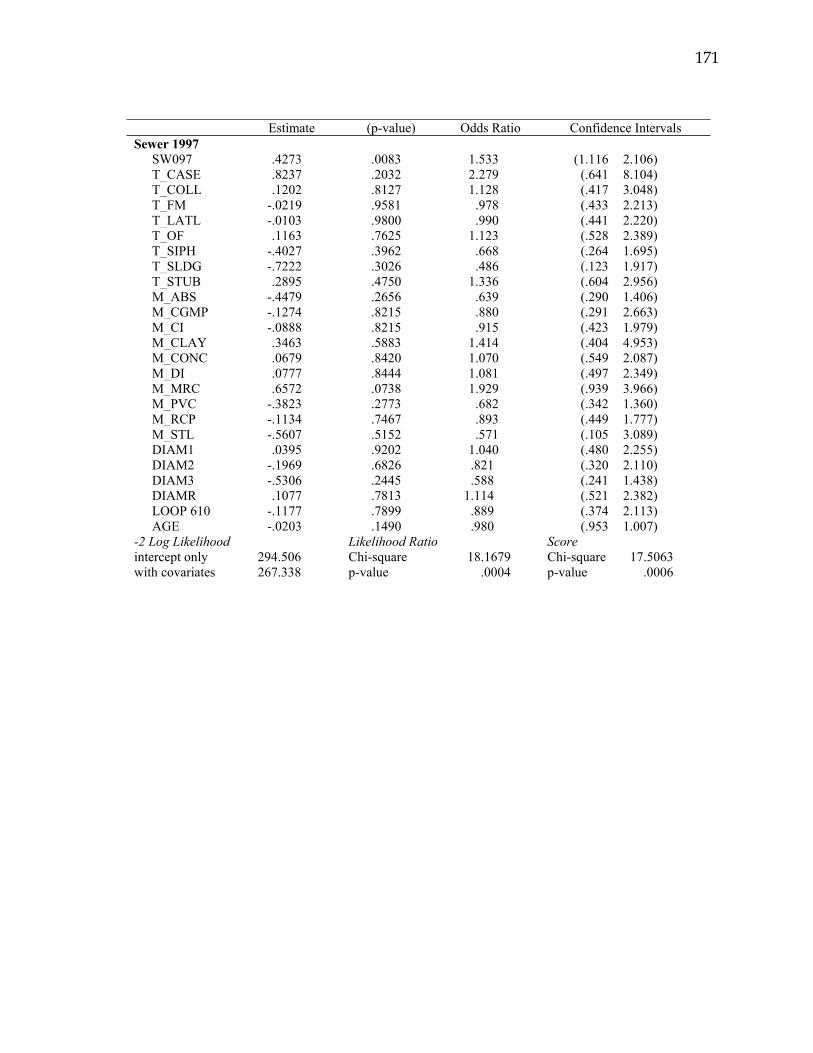
171

Estimate (p-value) Odds Ratio Confidence Intervals Sewer 1997 SW097 .4273 .0083 1.533 (1.116 2.106) T_CASE .8237 .2032 2.279 (.641 8.104) T_COLL .1202 .8127 1.128 (.417 3.048) T_FM -.0219 .9581 .978 (.433 2.213) T_LATL -.0103 .9800 .990 (.441 2.220) T_OF .1163 .7625 1.123 (.528 2.389) T_SIPH -.4027 .3962 .668 (.264 1.695) T_SLDG -.7222 .3026 .486 (.123 1.917) T_STUB .2895 .4750 1.336 (.604 2.956) M_ABS -.4479 .2656 .639 (.290 1.406) M_CGMP -.1274 .8215 .880 (.291 2.663) M_CI -.0888 .8215 .915 (.423 1.979) M_CLAY .3463 .5883 1.414 (.404 4.953) M_CONC .0679 .8420 1.070 (.549 2.087) M_DI .0777 .8444 1.081 (.497 2.349) M_MRC .6572 .0738 1.929 (.939 3.966) M_PVC -.3823 .2773 .682 (.342 1.360) M_RCP -.1134 .7467 .893 (.449 1.777) M_STL -.5607 .5152 .571 (.105 3.089) DIAM1 .0395 .9202 1.040 (.480 2.255) DIAM2 -.1969 .6826 .821 (.320 2.110) DIAM3 -.5306 .2445 .588 (.241 1.438) DIAMR .1077 .7813 1.114 (.521 2.382) LOOP 610 -.1177 .7899 .889 (.374 2.113) AGE -.0203 .1490 .980 (.953 1.007) -2 Log Likelihood Likelihood Ratio Score intercept only 294.506 Chi-square 18.1679 Chi-square 17.5063 with covariates 267.338 p-value .0004 p-value .0006

172

Estimate (p-value) Odds Ratio Confidence Intervals Sewer 1998 SW098 .2041 .3373 1.226 (.808 1.861) T_CASE .4081 .6916 1.504 (.200 11.295) T_COLL 2.8248 .0006 16.857 (3.355 84.686) T_FM .6846 .2331 .504 (.164 1.554) T_LATL .3885 .5737 1.475 (.431 5.042) T_OF .7297 .2150 .482 (.152 1.528) T_SIPH .9426 .0860 2.567 (.875 7.529) T_SLDG .2880 .7492 1.334 (.228 7.797) T_STUB -.6921 .2578 .501 (.151 1.660 M_ABS .8213 .1462 2.274 (.751 6.885) M_CGMP 1.1837 .0812 3.267 (.863 12.358) M_CI .4178 .4754 1.519 (.482 4.783) M_CLAY .0881 .9201 1.092 (.195 6.111) M_CONC .0551 .9108 1.057 (.403 2.768) M_DI -.5678 .3220 .567 (.184 1.743) M_MRC .2024 .7131 1.224 (.416 3.601) M_PVC -.2335 .6452 .792 (.293 2.139) M_RCP .0874 .8642 1.091 (.401 2.971) M_STL -.4085 .7472 .665 (.055 7.967) DIAM1 -.0754 .8902 .927 (.318 2.707) DIAM2 -.3716 .6001 .690 (.172 2.767) DIAM3 -.9792 .1353 .376 (.104 1.358) DIAMR -.5314 .3851 .588 (.177 1.950) LOOP 610 -.6603 .3614 .517 (.1252 .133) AGE -2 Log Likelihood Likelihood Ratio Score intercept only 183.698 Chi-square 17.2211 Chi-square 17.5990 with covariates 166.476 p-value .0002 p-value .0002

173

Estimate (p-value) Odds Ratio Confidence Intervals Sewer 1999 SW099 .5908 .0167 1.805 1.114 2.925 T_CASE -.2925 .1871 ..275 .040 1.873 T_COLL -.5755 .4567 .562 .124 2.560 T_FM -.4544 .4629 .635 .189 2.136 T_LATL -.2215 .7459 .801 .210 3.060 T_OF -.1302 .8130 .878 .298 2.583 T_SIPH .8977 .1304 2.454 .767 7.852 T_SLDG .7075 .3616 2.029 .444 9.276 T_STUB .4346 .4744 1.544 469 5.080 M_ABS -1.0503 .1350 .350 .088 1.387 M_CGMP .7000 .3374 2.014 .482 8.417 M_CI -.2723 .6467 .762 .238 2.441 M_CLAY .8167 .3314 2.263 .4361 1.760 M_CONC -.5833 .2548 .558 .205 1.523 M_DI -1.1312 .0751 .323 .093 1.121 M_MRC .5509 .3228 1.735 .582 5.171 M_PVC .7322 .1642 2.080 .741 5.835 M_RCP .6389 .2147 1.894 .690 5.197 M_STL -.1908 .8629 .826 .095 7.199 DIAM1 1.4067 .0162 4.083 1.297 12.847 DIAM2 .4479 .5382 1.565 .376 6.515 DIAM3 -.1658 .8003 .847 .234 3.061 DIAMR .1372 .8197 1.147 .353 3.730 LOOP 610 .3432 .6197 1.409 .364 5.464 AGE -.0292 .2009 .971 .929 1.016 -2 Log Likelihood Likelihood Ratio Score intercept only 183.698 Chi-square 20.7120 Chi-square 19.5195 with covariates 162.985 p-value .0001 p-value .0002

174

APPENDIX E: BIVARIATE ASSOCIATION OF POLITICAL VARIABLES

Water 1992 ACTIVE TEN STABLE VOTE ACTIVE C=-.0170 (.7419) K=2.463 (.2918) K=9.388 (.0246) TEN B=.0224 (.6284) B=.0787 (.4946) STABLE B=.0393 (.7262) DISTA C=.085 (.7701) K=142.7 (.0001) K=2.018 (.3645) K=1.268 (.7367) DISTB C=2.493 (.1143) K=18.18 (.0001) K=.7925 (.6728) K=1.153 (.7642) DISTC C=.6307 (.4271) K=15.15 (.0001) K=1.657 (.4367) K=6.043 (.1095) DISTD C=.0210 (.8847) K=177.4 (.0001) K=.4908 (.7824) K=3.011 (.3899) DISTE C=2.674 (.1020) K=13.47 (.0002) K=5.613 (.0604) K=2.691 (.4416) DISTF C=.0151 (.9022) K=8.291 (.0040) K= 1.018 (.6010) K=3.266 (.3523) DISTG C=.0021 (.9633) K=14.72 (.0001) K= 1.660 (.4360) K=2.604 (.4667) DISTH C=1.373 (.2413) K=21.80 (.0001) K= 1.084 (.5814) K=2.205 (.5309) DISTI C=.6307 (.4271) K=15.15 (.0001) K= .6105 (.7369) K=3.676 (.2986) 1993 ACTIVE TEN STABLE VOTE ACTIVE C=.0515(.6079) K=2.347 (.3092) K=10.84 (.0126) TENURE B=-.0387 (.4360) B=-.165 (.1381) STABLE B=.0448 (.6901) DISTA C=.0475 (.8276) K=142.7 (.0001) K=2.018 (.3645) K=1.709 (.6347) DISTB C=.0095 (.9225) K=30.14 (.0001) K=.7925 (.6728) K=.7790 (.8445) DISTC C=.1506 (.6979) K=25.11 (.0001) K=1.657 (.4367) K=4.601 (.2035) DISTD C=2.050 (.1521) K=177.4 (.0001) K=.4908 (.7824) K=1.744 (.6271) DISTE C=2.898 (.0887) K=22.34 (.0001) K=5.613 (.0604) K=4.417 (.2198) DISTF C=.0308 (.8606) K=13.74 (.0010) K=1.018 (.6010) K=3.923 (.2699) DISTG C=.0135 (.9073) K=24.41 (.0001) K= 1.660 (.4360) K=2.957 (.3982) DISTH C=5.079 (.0242) K=36.15 (.0001) K= 1.084 (.5814) K=2.503 (.4747) DISTI C=.1506 (.6979) K=374.0 (.0001) K= .6105 (.7369) K=3.046 (.3845) 1994

ACTIVE TEN STABLE VOTE ACTIVE C=.1086(.8170) K=2.214 (.3304) K=8.828 (.0317) TENURE B=-.0387 .4360) B=-.157 (.1573) STABLE B=-.018 (.8709) DISTA C=.2938 (.5878) K=142.7 (.0001) K=2.018 (.3645) K=2.413 (.4912) DISTB C=.1675 (.6823) K=30.14 (.0001) K=.7925 (.6728) K=.8694 (.8328) DISTC C=.5223 (.4699) K=25.11 (.0001) K=1.657 (.4367) K=3.753 (.2893) DISTD C=.6962 (.4041) K=177.4 (.0001) K=.4908 (.7824) K=1.592 (.6610) DISTE C=1.827 (.1764) K=22.34 (.0001) K=5.613 (.0604) K=2.879 (.4106) DISTF C=.3673 (.5445) K=13.74 (.0010) K=1.018 (.6010) K=3.571 (.3116) DISTG C=.3139 (.5753) K=24.41 (.0001) K= 1.660 (.4360) K=1.001 (.2613) DISTH C=.6306 (.4271) K=36.15 (.0001) K= 1.084 (.5814) K=2.407 (.4923) DISTI C=.1506 (.6979) K=374.0 (.0001) K= .6105 (.7369) K=2.580 (.4609) = Indicates significance at p=<.05

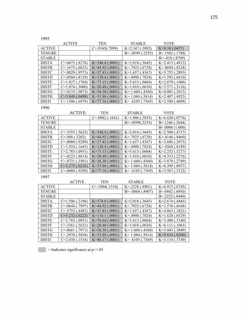
175

1995 ACTIVE TEN STABLE VOTE ACTIVE C=.0345(.7999) K=2.347 (.3092) K=8.10 (.0457) TENURE B=-.0599 (.2255) B=.1502 (.1788) STABLE B=-.018 (.8709) DISTA C=.0475 (.8276) K=346.4 (.0001) K=2.018 (.3645) K=2.413 (.4912) DISTB C=.1675 (.6823) K=44.92 (.0001) K=.7925 (.6728) K=.8694 (.8328) DISTC C=.0029 (.9573) K=37.43 (.0001) K=1.657 (.4367) K=3.753 (.2893) DISTD C=.0560 (.8129) K=120.4 (.0001) K=.4908 (.7824) K=1.592 (.6610) DISTE C=1.827 (.1764) K=73.15 (.0001) K=5.613 (.0604) K=2.879 (.1406) DISTF C=1.074 (.3000) K=20.48 (.0001) K=1.018 (.6010) K=3.571 (.3116) DISTG C=.0135 (.9073) K=36.38 (.0001) K= 1.660 (.4360) K=4.001 (.2613) DISTH C=3.849 (.0498) K=53.88 (.0001) K= 1.084 (.5814) K=2.407 (.4923) DISTI C=.1506 (.6979) K=77.16 (.0001) K= .6105 (.7369) K=2.580 (.4609) 1996 ACTIVE TEN STABLE VOTE ACTIVE C=.0982 (.1641) K=1.906 (.3855) K=6.828 (.0776) TENURE B=-.0599(.2255) B=.1246 (.2644) STABLE B=.0000 (1.000) DISTA C=.3355 (.5625) K=346.4 (.0001) K=2.018 (.3645) K=2.500 (.4717) DISTB C=.988 (.3202) K=44.92 (.0001) K=.7925 (.6728) K=.8146 (.8460) DISTC C=.0080 (.9289) K=37.43 (.0001) K=1.657 (.4367) K=3.686 (.2973) DISTD C=1.934 (.1643) K=120.4 (.0001) K=.4908 (.7824) K=.9268 (.8189) DISTE C=2.785 (.0951) K=73.15 (.0001) K=5.613 (.0604) K=2.252 (.5217) DISTF C=.0223 (.8814) K=20.48 (.0001) K=1.018 (.6010) K=4.333 (.2276) DISTG C=.8721 (.3501) K=36.38 (.0001) K= 1.660 (.4360) K=3.878 (.2749) DISTH C=5.275 (.0216) K=53.88 (.0001) K= 1.084 (.5814) K=6.399 (.0937) DISTI C=.0080 (.9289) K=77.16 (.0001) K= .6105 (.7369) K=3.567 (.3122) 1997 ACTIVE TEN STABLE VOTE ACTIVE C=.1004(.1510) K=.2328 (.8901) K=6.915 (.0745) TENURE B=-.0068 (.8907) B=.0442 (.6950) STABLE B=.2222 (.8440) DISTA C=1.506 (.2196) K=374.0 (.0001) K=2.018 (.3645) K=2.674 (.4445) DISTB C=.0644 (.7997) K=44.92 (.0001) K=.7925 (.6728) K=1.576 (.6648) DISTC C=.5752 (.4482) K=37.43 (.0001) K=1.657 (.4367) K=4.863 (.1821) DISTD C=5.232 (.0222) K=116.1 (.0001) K=.4908 (.7824) K=1.628 (.6529) DISTE C=2.785 (.0951) K=76.64 (.0001) K=5.613 (.0604) K=3.400 (.3340) DISTF C=.3361 (.5621) K=20.48 (.0001) K=1.018 (.6010) K=6.111 (.1063) DISTG C=.0661 (.7971) K=36.38 (.0001) K= 1.660 (.4360) K=3.043 (.3849) DISTH C=.2970 (.5858) K=53.88 (.0001) K= 1.084 (.5814) K=9.834 (.0200) DISTI C=2.038 (.1534) K=86.17 (.0001) K= .6105 (.7369) K=3.110 (.3749) = Indicates significance at p=<.05

176

1998 ACTIVE TEN STABLE VOTE ACTIVE C=.1692(.0047) K=.7093 (.7014) K=7.347 (.0616) TENURE B=-.0068 (.8907) B=.0536 (.6348) STABLE B=.0139 (.9021) DISTA C=3.519 (.0607) K=374.0 (.0001) K=2.018 (.3645) K=2.455 (.4835) DISTB C=.4653 (.4951) K=44.92 (.0001) K=.7925 (.6728) K=2.092 (.5534) DISTC C=.0602 (.8062) K=37.43 (.0001) K=1.657 (.4367) K=6.739 (.0807) DISTD C=6.688 (.0097) K=116.1 (.0001) K=.4908 (.7824) K=1.951 (.5826) DISTE C=5.617 (.0178) K=76.64 (.0001) K=5.613 (.0604) K=3.199 (.3619) DISTF C=.0791 (.7785) K=20.48 (.0001) K=1.018 (.6010) K=6.111 (.1063) DISTG C=1.618 (.2033) K=36.38 (.0001) K=1.660 (.4360) K=2.755 (.4308) DISTH C=4.019 (.0450) K=53.88 (.0001) K=1.084 (.5814) K=9.899 (.0164) DISTI C=.1796 (.6717) K=86.17 (.0001) K= .6105 (.7369) K=3.302 (.3472) 1999 ACTIVE TEN STABLE VOTE ACTIVE C=.1173(.0758) K=1.871 (.3924) K=10.60 (.0140) TENURE B=.0532 (.2830) B=.0385 (.7319) STABLE B=-.001 (.9674) DISTA C=2.982 (.0841) K=374.0 (.0001) K=2.018 (.3645) K=2.733 (.4346) DISTB C=.0461 (.8301) K=44.92 (.0001) K=.7925 (.6728) K=2.669 (.4454) DISTC C=2.980 (.0843) K=37.43 (.0001) K=1.657 (.4367) K=6.715 (.0815) DISTD C=.6962 (.4041) K=116.1 (.0001) K=.4908 (.7824) K=2.326 (.5075) DISTE C=1.827 (.1764) K=76.64 (.0001) K=5.613 (.0604) K=2.297 (.5131) DISTF C=.3673 (.5445) K=20.48 (.0001) K=1.018 (.6010) K=4.818 (.1856) DISTG C=2.481 (.1152) K=36.38 (.0001) K=1.660 (.4360) K=2.847 (.4158) DISTH C=.0442 (.8335) K=53.88 (.0001) K=1.084 (.5814) K=7.470 (.0583) DISTI C=.5223 (.4699) K=86.17 (.0001) K= .6105 (.7369) K=3.768 (.2876) = Indicates significance at p=<.05

177

Sewer 1992 ACTIVE TEN STABLE VOTE ACTIVE C=-.121 (.0188) K=2.184 (.3355) K=5.949 (.1141) TEN B=.0249 (.6284) B=.0787 (.4946) STABLE B=.0393 (.7262) DISTA C=1.030 (.3100) K=142.7 (.0001) K=.2018 (.3645) K=.0999 (.7519) DISTB C=.3193 (.5720) K=18.18 (.0001) K=.7925 (.6728) K=.5733 (.4489) DISTC C=.0191 (.8900) K=15.15 (.0001) K=1.657 (.4367) K=1.858 (.1728) DISTD C= 4.087(.0432) K=177.4 (.0001) K=.4908 (.7824) K=1.021 (.3123) DISTE C=.0174 (.8685) K=13.47 (.0002) K=5.613 (.0406) K=.0730 (.7871) DISTF C=.8673 (.3517) K=8.291 (.0040) K=1.018 (.6010) K=1.888 (.1694) DISTG C=2.782 (.0953) K=14.72 (.0001) K=1.660 (.4360) K=1.364 (.2427) DISTH C=1.163 (.2807) K=21.80 (.0001) K=1.084 (.5814) K=1.300 (.2541) DISTI C=1.441 (.2299) K=15.15 (.0001) K=.6015 (.7369) K=1.940 (.1636) 1993 ACTIVE TEN STABLE VOTE ACTIVE C=.1396(.0258) K=2.214 (.3458) K=5.706 (.1268) TENURE B=-.0387(.4360) B=-.181 (.1043) STABLE B=.0448 (.6901) DISTA C=.1018 (.7497) K=57.37 (.0001) K=.2018 (.3645) K=.0998 (.7521) DISTB C=.0853 (.7702) K=28.95 (.0001) K=.7925 (.6728) K=.0636 (.8009) DISTC C=.2453 (.6204) K=24.10 (.0001) K=1.657 (.4367) K=2.158 (.1418) DISTD C=5.194 (.0227) K=71.32 (.0001) K=.4908 (.7824) K=.5038 (.4778) DISTE C=.3024 (.5824) K=21.43 (.0001) K=5.613 (.0406) K=.3247 (.5688) DISTF C=1.926 (.1651) K=13.18 (.0003) K=1.018 (.6010) K=2.042 (.1530) DISTG C=7.389 (.0066) K=23.42 (.0001) K=1.660 (.4360) K=1.440 (.2300) DISTH C=.0022 (.9627) K=34.69 (.0001) K=1.084 (.5814) K=1.481 (.2235) DISTI C=3.363 (.0997) K=148.4 (.0001) K=.6015 (.7369) K=2.127 (.1447) 1994 ACTIVE TEN STABLE VOTE ACTIVE C=.1600(.0082) K=4.123 (.1273) K=2.764 (.4293) TENURE B=-.0387 .4360) B=-.1811(.1043) STABLE B=-.018 (.8709) DISTA C=1.50 (.2196) K=57.37 (.0001) K=.2018 (.3645) K=.1849 (.6672) DISTB C=.4653 (.4951) K=28.95 (.0001) K=.7925 (.6728) K=.0552 (.8142) DISTC C=.1796 (.6717) K=24.10 (.0001) K=1.657 (.4367) K=3.005 (.0830) DISTD C=3.597 (.0579) K=71.32 (.0001) K=.4908 (.7824) K=.7368 (.3907) DISTE C=1.738 (.1874) K=21.43 (.0001) K=5.613 (.0406) K=.1757 (.6751) DISTF C=2.075 (.1497) K=13.18 (.0003) K=1.018 (.6010) K=1.956 (.1618) DISTG C=2.058 (.1514) K=23.42 (.0001) K=1.660 (.4360) K=1.724 (.1891) DISTH C=.3879 (.5334) K=34.69 (.0001) K=1.084 (.5814) K=2.367 (.1239) DISTI C=2.038 (.1534) K=148.4 (.0001) K=.6015 (.7369) K=1.779 (.1822) = Indicates significance at p=<.05

178

1995 ACTIVE TEN STABLE VOTE ACTIVE C=.1131(.0907) K=14.95 (.0600) K=4.911 (.1784) TENURE B=-.059 (.2255) B=.2041 (.0682) STABLE B=.0000 (1.000) DISTA C=.9563 (.3281) K=139.7 (.0001) K=.2018 (.3645) K=.1849 (.6672) DISTB C=.0004 (.9841) K=8.917 (.0028) K=.7925 (.6728) K=.0552 (.8142) DISTC C=.2453 (.6204) K=7.430 (.0064) K=1.657 (.4367) K=3.005 (.0830) DISTD C=3.920 (.0477) K=100.3 (.0001) K=.4908 (.7824) K=.7368 (.3907) DISTE C=1.565 (.2018) K=57.94 (.0001) K=5.613 (.0406) K=.1757 (.6751) DISTF C=1.926 (.1651) K=4.066 (.0437) K=1.018 (.6010) K=1.956 (.1618) DISTG C=-5.663 (.0173) K=7.223 (.0072) K=1.660 (.4360) K=1.724 (.1891) DISTH C=.2887 (.5910) K=10.69 (.0011) K=1.084 (.5814) K=2.367 (.1239) DISTI C=2.248 (.1338) K=58.17 (.0001) K=.6015 (.7369) K=1.779 (.1822) 1996 ACTIVE TEN STABLE VOTE ACTIVE C=.0646(.4571) K=4.204 (.1222) K=8.284 (.0405) TENURE B=-.0599 (.2255) B=.2041(.0682) STABLE B=.0000 (1.000) DISTA C=.0010 (.9745) K=139.7 (.0001) K=.2018 (.3645) K=.1396 (.7087) DISTB C=.0004 (.9847) K=8.917 (.0028) K=.7925 (.6728) K=.1631 (.6863) DISTC C=.6307 (.4271) K=7.430 (.0064) K=1.657 (.4367) K=2.836 (.0922) DISTD C=2.688 (.1011) K=100.3 (.0001) K=.4908 (.7824) K=.4100 (.5220) DISTE C=.8726 (.3502) K=57.94 (.0001) K=5.613 (.0406) K=.1025 (.7489) DISTF C=.3062 (.5800) K=4.066 (.0437) K=1.018 (.6010) K=2.126 (.1448) DISTG C=4.311 (.3079) K=7.223 (.0072) K=1.660 (.4360) K=1.647 (.1993) DISTH C=.0000 (.9969) K=10.69 (.0011) K=1.084 (.5814) K=4.246 (.0393) DISTI C=.6307 (.4271) K=58.17 (.0001) K=.6015 (.7369) K=1.192 (.2748) 1997 ACTIVE TEN STABLE VOTE ACTIVE C=.0977(.1672) K=14.50 (.0696) K=8.437 (.0378) TENURE B=-.0068 (.8907) B=.1214 (.2802) STABLE B=.02122(.8440) DISTA C=.3800 (.5376) K=142.7 (.0001) K=.2018 (.3645) K= .4819 (.4876) DISTB C=.0004 (.9847) K=41.90 (.0001) K=.7925 (.6728) K=.0141 (.9056) DISTC C=.0156 (.9006) K=34.92 (.0001) K=1.657 (.4367) K=4.108 (.0427) DISTD C=1.797 (.1800) K=41.73 (.0001) K=.4908 (.7824) K=.3068 (.5797) DISTE C=.8726 (.3502) K=27.53 (.0001) K=5.613 (.0406) K=.1705 (.6797) DISTF C=2.005 (.1573) K=19.10 (.0001) K=1.018 (.6010) K=2.410 (.1205) DISTG C=7.579 (.0059) K=33.94 (.0001) K=1.660 (.4360) K=1.382 (.2396) DISTH C=.3456 (.5566) K=50.26 (.0001) K=1.084 (.5814) K=5.092 (.0240) DISTI C=3.233 (.0722) K=30.95 (.0001) K=.6015 (.7369) K=1.722 (.1894) = Indicates significance at p=<.05

179

1998 ACTIVE TEN STABLE VOTE ACTIVE C=.1151 (.0834) K=18.40 (.0184) K=10.85 (.0126) TENURE B=-.0068 (.9807) B= .0836 (.6348) STABLE B=.0139 (.9021) DISTA C=.3355 (.5625) K=142.7 (.0001) K=.2018 (.3645) K=.4431 (.5056) DISTB C=.1370 (.7112) K=41.90 (.0001) K=.7925 (.6728) K=.0026 (.9595) DISTC C=1.194 (.2744) K=34.92 (.0001) K=1.657 (.4367) K=4.993 (.0254) DISTD C=3.597 (.0579) K=41.73 (.0001) K=.4908 (.7824) K=.3534 (.5522) DISTE C=.9364 (.3332) K=27.53 (.0001) K=5.613 (.0406) K=.1390 (.7093) DISTF C=3.501 (.0613) K=19.10 (.0001) K=1.018 (.6010) K=2.413 (.1203) DISTG C=7.773 (.0053) K=33.94 (.0001) K=1.660 (.4360) K=1.307 (.2528) DISTH C=.0015 (.9689) K=50.26 (.0001) K=1.084 (.5814) K=5.158 (.0231) DISTI C=3.105 (.0780) K=30.95 (.0001) K=.6015 (.7369) K=1.783 (.1817) 1999 ACTIVE TEN STABLE VOTE ACTIVE C=.1151(.0834) K=18.40 (.0184) K=11.02 (.0116) TENURE B=.0531 (.2830) B=-.150 (.1804) STABLE B=-.004 (.9674) DISTA C=.3355 (.5625) K=7.482 (.0062) K=.2018 (.3645) K=.5186 (.4715) DISTB C=.1370 (.7112) K=41.90 (.0001) K=.7925 (.6728) K=.4666 (.4946) DISTC C=1.194 (.2744) K=34.92 (.0001) K=1.657 (.4367) K=5.187 (.0227) DISTD C=3.597 (.0579) K=98.23 (.0001) K=.4908 (.7824) K=.2415 (.6231) DISTE C=.9364 (.3332) K=64.79 (.0001) K=5.613 (.0406) K=.6762 (.4109) DISTF C=3.501 (.0613) K=19.10 (.0001) K=1.018 (.6010) K=2.219 (.1363) DISTG C=7.773 (.0053) K=33.94 (.0001) K=1.660 (.4360) K=1.371 (.2416) DISTH C=.0015 (.9689) K=50.26 (.0001) K=1.084 (.5814) K=4.650 (.0310) DISTI C=3.105 (.0780) K=72.85 (.0001) K=.6015 (.7369) K=1.482 (.2234) = Indicates significance at p=<.05

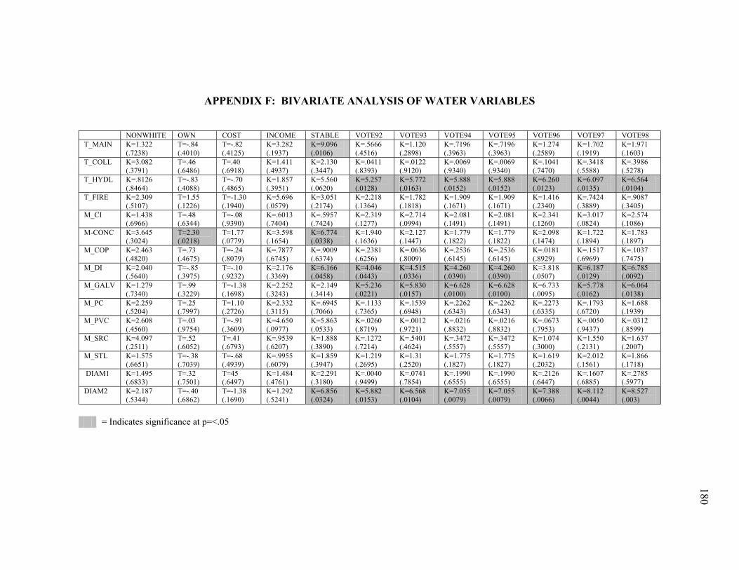
180

APPENDIX F: BIVARIATE ANALYSIS OF WATER VARIABLES

NONWHITE OWN COST INCOME STABLE VOTE92 VOTE93 VOTE94 VOTE95 VOTE96 VOTE97 VOTE98 T_MAIN K=1.322

(.7238) T=-.84 (.4010)

T=-.82 (.4125)

K=3.282 (.1937)

K=9.096 (.0106)

K=.5666 (.4516)

K=1.120 (.2898)

K=.7196 (.3963)

K=.7196 (.3963)

K=1.274 (.2589)

K=1.702 (.1919)

K=1.971 (.1603)

T_COLL K=3.082 (.3791)

T=.46 (.6486)

T=.40 (.6918)

K=1.411 (.4937)

K=2.130 (.3447)

K=.0411 (.8393)

K=.0122 (.9120)

K=.0069 (.9340)

K=.0069 (.9340)

K=.1041 (.7470)

K=.3418 (.5588)

K=.3986 (.5278)

T_HYDL K=.8126 (.8464)

T=-.83 (.4088)

T=-.70 (.4865)

K=1.857 (.3951)

K=5.560 (.0620)

K=5.257 (.0128)

K=5.772 (.0163)

K=5.888 (.0152)

K=5.888 (.0152)

K=6.260 (.0123)

K=6.097 (.0135)

K=6.564 (.0104)

T_FIRE K=2.309 (.5107)

T=1.55 (.1226)

T=-1.30 (.1940)

K=5.696 (.0579)

K=3.051 (.2174)

K=2.218 (.1364)

K=1.782 (.1818)

K=1.909 (.1671)

K=1.909 (.1671)

K=1.416 (.2340)

K=.7424 (.3889)

K=.9087 (.3405)

M_CI K=1.438 (.6966)

T=.48 (.6344)

T=-.08 (.9390)

K=.6013 (.7404)

K=.5957 (.7424)

K=2.319 (.1277)

K=2.714 (.0994)

K=2.081 (.1491)

K=2.081 (.1491)

K=2.341 (.1260)

K=3.017 (.0824)

K=2.574 (.1086)

M-CONC K=3.645 (.3024)

T=2.30 (.0218)

T=1.77 (.0779)

K=3.598 (.1654)

K=6.774 (.0338)

K=1.940 (.1636)

K=2.127 (.1447)

K=1.779 (.1822)

K=1.779 (.1822)

K=2.098 (.1474)

K=1.722 (.1894)

K=1.783 (.1897)

M_COP K=2.463 (.4820)

T=.73 (.4675)

T=-.24 (.8079)

K=.7877 (.6745)

K=.9009 (.6374)

K=.2381 (.6256)

K=.0636 (.8009)

K=.2536 (.6145)

K=.2536 (.6145)

K=.0181 (.8929)

K=.1517 (.6969)

K=.1037 (.7475)

M_DI K=2.040 (.5640)

T=-.85 (.3975)

T=-.10 (.9232)

K=2.176 (.3369)

K=6.166 (.0458)

K=4.046 (.0443)

K=4.515 (.0336)

K=4.260 (.0390)

K=4.260 (.0390)

K=3.818 (.0507)

K=6.187 (.0129)

K=6.785 (.0092)

M_GALV K=1.279 (.7340)

T=.99 (.3229)

T=-1.38 (.1698)

K=2.252 (.3243)

K=2.149 (.3414)

K=5.236 (.0221)

K=5.830 (.0157)

K=6.628 (.0100)

K=6.628 (.0100)

K=6.733 (.0095)

K=5.778 (.0162)

K=6.064 (.0138)

M_PC K=2.259 (.5204)

T=.25 (.7997)

T=1.10 (.2726)

K=2.332 (.3115)

K=.6945 (.7066)

K=.1133 (.7365)

K=.1539 (.6948)

K=.2262 (.6343)

K=.2262 (.6343)

K=.2273 (.6335)

K=.1793 (.6720)

K=1.688 (.1939)

M_PVC K=2.608 (.4560)

T=.03 (.9754)

T=-.91 (.3609)

K=4.650 (.0977)

K=5.863 (.0533)

K=.0260 (.8719)

K=.0012 (.9721)

K=.0216 (.8832)

K=.0216 (.8832)

K=.0673 (.7953)

K=.0050 (.9437)

K=.0312 (.8599)

M_SRC K=4.097 (.2511)

T=.52 (.6052)

T=.41 (.6793)

K=.9539 (.6207)

K=1.888 (.3890)

K=.1272 (.7214)

K=.5401 (.4624)

K=.3472 (.5557)

K=.3472 (.5557)

K=1.074 (.3000)

K=1.550 (.2131)

K=1.637 (.2007)

M_STL K=1.575 (.6651)

T=-.38 (.7039)

T=-.68 (.4939)

K=.9955 (.6079)

K=1.859 (.3947)

K=1.219 (.2695)

K=1.31 (.2520)

K=1.775 (.1827)

K=1.775 (.1827)

K=1.619 (.2032)

K=2.012 (.1561)

K=1.866 (.1718)

DIAM1

K=1.495 (.6833)

T=.32 (.7501)

T=45 (.6497)

K=1.484 (.4761)

K=2.291 (.3180)

K=.0040 (.9499)

K=.0741 (.7854)

K=.1990 (.6555)

K=.1990 (.6555)

K=.2126 (.6447)

K=.1607 (.6885)

K=.2785 (.5977)

DIAM2

K=2.187 (.5344)

T=-.40 (.6862)

T=-1.38 (.1690)

K=1.292 (.5241)

K=6.856 (.0324)

K=5.882 (.0153)

K=6.568 (.0104)

K=7.055 (.0079)

K=7.055 (.0079)

K=7.388 (.0066)

K=8.112 (.0044)

K=8.527 (.003)

= Indicates significance at p=<.05

181

VOTE99 ACTIVE92 ACTIVE93 ACTIVE94 ACTIVE95 ACTIVE96 ACTIVE97 ACTIVE98 ACTIVE99 TEN92 TEN93 TEN94 T_MAIN K=2.515

(.1128) C=.2639 (.0001)

C=.2533 (.0001)

C=.3280 (.0001)

C=.3280 (.0001)

C=.2693 (.0001)

C=.3119 (.0001)

C=.2799 (.0001)

C=.3173 (.0001)

K=.2528 (.6151)

K=.9267 (.3357)

K=.9267 (.3357)

T_COLL K=.2678 (.6048)

C=-.048 (.3502)

C=-.067 (.1928)

C=-.038 (.4513)

C=-.010 (.8382)

C=-.022 (.6658)

C=-.050 (.3266)

C=-.022 (.6658)

C=-.024 (.6321)

K=1.424 (.2327)

K=.0020 (.9643)

K=.0020 (.9643)

T_HYDL K=7.423 (.0064)

C=.2267 (.0001)

C=.2160 (.0001)

C=.2587 (.0001)

C=.2907 (.0001)

C=.2320 (.0001)

C=.2533 (.0001)

C=.2640 (.0001)

C=-.301 (.0001)

K=.1061 (.7447)

K=.0004 (.9843)

K=.0004 (.9843)

T_FIRE K=1.927 (.1651)

C=-.004 (.9317)

C=-.089 (.0843)

C=-.003 (.9471)

C=-.024 (.6303)

C=.0121 (.8141)

C=.0229 (.6580)

C=.0657 (.2032)

C=-.003 (.9471)

K=1.456 (.2275)

K=.2137 (.6439)

K=.2137 (.6439)

M_CI K=3.016 (.0824)

C=.1733 (.0008)

C=.1413 (.0062)

C=.1093 (.0343)

C=.1627 (.0016)

C=.1466 (.0045)

C=.1573 (.0023)

C=.1573 (.0023)

C=.1200 (.0202)

K=6.351 (.0117)

K=11.09 (.0009)

K=11.097 (.0009)

M-CONC K=1.482 (.2234)

C=.0153 (.7672)

C=-.007 (.8879)

C=-.007 (.8879)

C=-.026 (.6058)

C=.0137 (.7910)

C=.0137 (.7910)

C=.0524 (.3100)

C=.0121 (.8150)

K=.2438 (.6215)

K=2.827 (.0927)

K=2.827 (.0927)

M_COP K=.1778 (.6733)

C=.0929 (.0719)

C=.1508 (.0035)

C=.1636 (.0015)

C=.1890 (.0003)

C=.0391 (.4493)

C=.1028 (.0466)

C=.1537 (.0029)

C=.0234 (.6499)

K=.1886 (.6641)

K=.8808 (.3709)

K=.8008 (.3709)

M_DI K=6.136 (.0132)

C=-.040 (.4331)

C=-.024 (.6418)

C=-.070 (.1706)

C=-.024 (.6418)

C=-.020 (.6905)

C=-.008 (.8635)

C=-.032 (.5323)

C=.0227 (.6601)

K=.0523 (.8192)

K=1.913 (.1666)

K=1.913 (.1666)

M_GALV K=5.937 (.0148)

C=.2125 (.0001)

C=.2042 (.0001)

C=.2152 (.0001)

C=.2262 (.0001)

C=.1864 (.0003)

C=.1864 (.0003)

C=.1644 (.0015)

C=.0612 (.2358)

K=1.478 (.2241)

K=7.858 (.0051)

K=7.858 (.0051)

M_PC K=1.672 (.1960)

C=.0567 (.2720)

C=.0281 (.5866)

C=.0809 (.1174)

C=.1072 (.0378)

C=.0820 (.1124)

C=.0820 (.1124)

C=.1612 (.0018)

C=.0545 (.2915)

K=.3085 (.5786)

K=.0004 (.9834)

K=.0004 (.9834)

M_PVC K=.2151 (.6428)

C=.1945 (.0002)

C=.1519 (.0033)

C=.2053 (.0001)

C=.2266 (.0001)

C=.1679 (.0012)

C=.1892 (.0002)

C=.1465 (.0046)

C=.1412 (.0062)

K=.0010 (.9748)

K=3.772 (.0521)

K=3.772 (.0521)

M_SRC K=2.376 (.1232)

C=-.064 (.2117)

C=-.047 (.3566)

C=-.027 (.5926)

C=-.007 (.8820)

C=-.066 (.2010)

C=-.066 (.2010)

C=-.046 (.3724)

C=-.007 (.8820)

K=.0841 (.7718)

K=1.683 (.1945)

K=1.683 (.1945)

M_STL K=2.025 (.1547)

C=-.090 (.0791)

C=-.101 (.0498)

C=-.086 (.0949)

C=-.025 (.6156)

C=-.028 (.5858)

C=-.088 (.0867)

C=-.133 (.0096)

C=-.010 (.8335)

K=.1278 (.7207)

K=.1110 (.7390)

K=.1110 (.7390)

DIAM1

K=.2614 (.6092)

C=.2800 (.0001)

C=.2800 (.0001)

C=.2480 (.0001)

C=.3013 (.0001)

C=.2533 (.0001)

C=.2533 (.0001)

C=.2427 (.0001)

C=.1947 (.0002)

K=.0221 (.8819)

K=9.203 (.0024)

K=9.203 (.0024)

DIAM2

K=9.578 (.0020)

C=.2907 (.0001)

C=.2693 (.0001)

C=.3120 (.0001)

C=.2907 (.0001)

C=.2853 (.0001)

C=.3173 (.0001)

C=.2640 (.0001)

C=.3120 (.0001)

K=.1061 (.7447)

K=.0803 (.7768)

K=.0803 (.7768)

= Indicates significance at p=<.05

182

TEN95 TEN96 TEN97 TEN98 TEN99 DISTA DISTB DISTC DISTD DISTE DISTF T_MAIN K=2.410

(.1205) K=2.410 (.1205)

K=2.548 (.1104)

K=2.548 (.1104)

K=4.316 (.0377)

C=-.005 (.9153)

C=-.107 (.0490)

C=-.1009 (.0507)

C=-.0277 (.5923)

C=.1112 (.0312)

C=.0354 (.4932)

T_COLL K=2.281 (.1309)

K=2.281 (.1309)

K=.5732 (.4490)

K=.5732 (.4490)

K=.1045 (.7465)

C=.1037 (.0446)

C=-.064 (.2104)

C=.0499 (.3339)

C=-.017 (.7283)

C=-.0035 (.9465)

C=.0317 (.5387)

T_HYDL K=.0054 (.9414)

K=.0054 (.9414)

K=2.029 (.1543)

K=2.029 (.1543)

K=1.604 (.2052)

C=.0428 (.4071)

C=-.071 (.1663)

C=-.050 (.3242)

C=-.060 (.2401)

C=.1276 (.0135)

C=.0563 (.2760)

T_FIRE K=4.325 (.0375)

K=4.325 (.0375)

K=.3298 (.5658)

.3298 (.5658)

K=1.542 (.2143)

C=.0421 (.4144)

C=-.053 (.3002)

C=.0150 (.7709)

C=-.117 (.0230)

C=-.024 (.6421)

C=.1021 (.0480)

M_CI K=3.206 (.0734)

K=3.206 (.0734)

K=3.221 (.0727)

K=3.221 (.0727)

K=.2466 (.6195)

C=.1432 (.0055)

C=-.039 (.4471)

C=-.120 (.0201)

C=.0319 (.5363)

C=-.180 (.0005)

C=-.077 (.1353)

M-CONC K=.1018 (.7496)

K=.1018 (.7496)

K=1.346 (.2460)

K=1.346 (.2460)

K=.8464 (.3576)

C=.0439 (.3950)

C=.0034 (.9482)

C=.0218 (.6736)

C=-.008 (.8713)

C=-.032 (.5344)

C=-.076 (.1373)

M_COP K=1.866 (.1719)

K=1.866 (.1719)

K=.4338 (.5101)

K=.4338 (.5101)

K=1.294 (.2553)

C=.0251 (.6275)

C=-.031 (.5380)

C=-.042 (.4089)

C=-.051 (.3200)

C=-.133 (.0099)

C=-.138 (.0074)

M_DI K=.0653 (.7983)

K=.0653 (.7983)

K=2.146 (.1429)

K=2.146 (.1429)

K=1.774 (.1829)

C=.0417 (.4199)

C=-.033 (.5136)

C=.0220 (.6708)

C=-.023 (.6487)

C=.0267 (.6058)

C=-.044 (.3940)

M_GALV K=6.674 (.0098)

K=6.674 (.0098)

K=.2088 (.6477)

K=.2088 (.6477)

K=.9438 (.3313)

C=-.125 (.0150)

C=-.013 (.7977)

C=-.145 (.0050)

C=.0367 (.4768)

C=-.142 (.0058)

C=-.199 (.0001)

M_PC K=4.477 (.0343)

K=4.477 (.0343)

K=.0063 (.9369)

K=.0063 (.9369)

K=1.448 (.2288)

C=.0897 (.0825)

C=-.040 (.4379)

C=.0125 (.8082)

C=-.046 (.3676)

C=-.068 (.1828)

C=-.0560 (.2780)

M_PVC K=7.038 (.0080)

K=7.038 (.0080)

K=1.312 (.2519)

K=1.312 (.2519)

K=5.339 (.0208)

C=-.070 (.1720)

C=-.115 (.0250)

C=.0046 (.9289)

C=.0671 (.1939)

C=.0225 (.6637)

C=.0966 (.0613)

M_SRC K=.9701 (.3247)

K=.9701 (.3247)

K=.3869 (.5339)

K=.3869 (.5339)

K=1.088 (.2968)

C=.0211 (.6823)

C=-.019 (.7110)

C=-.003 (.9534)

C=-.0006 (.9905)

C=.0073 (.8873)

C=.1340 (.0094)

M_STL K=1.003 (.3164)

K=1.003 (.3164)

K=.1070 (.7435)

K=.1070 (.7435)

K=.1387 (.7096)

C=-.063 (.2172)

C=-.093 (.0702)

C=.0212 (.6819)

C=.0355 (.4921)

C=.0328 (.5259)

C=.0431 (.4035)

DIAM1

K=2.034 (.1538)

K=2.034 (.1538)

K=.4980 (.4804)

K=.4980 (.4804)

K=1.405 (.2357)

C=-.024 (.6400)

C=.0574 (.2664)

C=-.189 (.0002)

C=.0319 (.5363)

C=-.125 (.0148)

C=-.143 (.0054)

DIAM2

K=.5162 (.4725)

.5162 (.4725)

K=2.281 (.1309)

K=2.281 (.1309)

K=2.499 (.1139)

C=.0261 (.6137)

C=-.119 (.0203)

C=-.033 (.5148)

C=-.045 (.3811)

C=.1276 (.0135)

C=.0563 (.2760)

= Indicates significance at p=<.05

183

DISTG DISTH DISTI T_MAIN C=-.006

(.9073) C=.0259 (.6156)

C=.0892 (.0843)

T_COLL C=-.015 (.7680)

C=-.007 (.8807)

C=-.064 (.2088)

T_HYDL C=.0970 (.0603)

C=-.112 (.0301)

C= .0182 (.7245)

T_FIRE C=.0758 (.1421)

C=-.029 (.5708)

C=.0324 (.5305)

M_CI C=-.042 (.4075)

C=.1443 (.0052)

C=.0873 (.0909)

M-CONC C=-.102 (.0476)

C=.0398 (.4411)

C=.0845 (.1018)

M_COP C=-.038 (.4572)

C=.2617 (.0001)

C=.0812 (.1160)

M_DI C=-.029 (.5672)

C=-.037 (.4660)

C=.078 (.1274)

M_GALV C=-.121 (.0183)

C=.3601 (.0001)

C=.2467 (.0001)

M_PC C=.0145 (.7785)

C=.0244 (.6370)

C=-.030 (.5586)

M_PVC C=.0308 (.5515)

C=.0131 (.8002)

C=.1256 (.0150)

M_SRC C=-.033 (.5199)

C=.0211 (.6833)

C=-.100 (.0527)

M_STL C=-.031 (.5405)

C=.0653 (.2058)

C=-.0033 (.9497)

DIAM1

C=-.1476 (.0043)

C=.2649 (.0001)

C=.1910 (.0002)

DIAM2

C=.0795 (.1235)

C=-.081 (.1131)

C=.0355 (.4921)

= Indicates significance at p=<.05

184

NONWHITE OWN COST INCOME STABLE VOTE92 VOTE93 VOTE94 VOTE95 VOTE96 VOTE97 DIAM3 K=5.9544

(.1136) T=-.49 (.1381)

T=-2.55 (.0113)

K=8.906 (.0116)

K=6.856 (.0324)

K=.0980 (.7543)

K=.6169 (.4322)

K=.3318 (.5646)

K=.3318 (.5646)

K=.6624 (.4157)

K=.5100 (.4751)

DIAM4 K=2.604 (.4067)

T=-.56 (.5740)

T=-1.04 (.2968)

K=1.641 (.4402)

K=3.354 (.1869)

K=4.572 (.0325)

K=3.986 (.0459)

K=4.854 (.0276)

K=4.854 (.0276)

K=4.219 (.0400)

K=4.188 (.0407)

DIAM5 K=8.632 (.0346)

T=.81 (.4178)

T=-.43 (.6649)

K=2.070 (.3551)

K=.8182 (.6642)

K=.0777 (.7804)

K=.0939 (.7593)

K=.3251 (.5686)

K=.3251 (.5686)

K=.6313 (.4269)

K=1.228 (.2677)

LOOP 610

K=6.420 (.0929)

T=.51 (.6117)

T=-4.60 (.0001)

K=17.57 (.0002)

K=.6788 (.7122)

K=5.982 (.0145)

K=6.409 (.0114)

K=6.169 (.0130)

K=6.169 (.0130)

K=6.053 (.0139)

K=4.824 (.0281)

AGE B=.1183 (.0028)

B=.0105 (.7674)

B=-.203 (.0001)

B=-.232 (.0001)

B=-.067 (.1183)

B=-.208 (.0317)

B=-.163 (.0913)

B=-.170 (.0787)

B=-.170 (0787)

B=-.134 (.1651)

B=-.143 (.1415)

NON WHITE

B=-.041 (.3740)

B=.0310 (.7690)

B=-.003 (.9751)

B=-.038 (.7130)

B=-.038 (.7130)

B=-.046 (.6573)

B=-.050 (.6371)

OWN

B=-.046 (.2698)

B=.1362 (.1538)

B=.1348 (.1576)

B=.1465 (.1243)

B=.1465 (.1243)

B=.1333 (.1626)

B=.1284 (.1806)

COST

B=.0329 (.4522)

B=-.053 (.5902)

B=-.026 (.7902)

B=-.000 (.9952)

B=-.000 (.9952)

B=.0065 (.9569)

B=.029 (.7653)

INCOME

B=-.007 (.8810)

B=-.053 (.6374)

B=-.010 (.9272)

B=-.019 (.8662)

B=-.019 (.8662)

B=.0063 (.9551)

B=-.003 (.9774)

= Indicates significance at p=<.05

185

VOTE98 VOTE99

ACTIVE 92

ACTIVE 93

ACTIVE 94

ACTIVE 95

ACTIVE 96

ACTIVE 97

ACTIVE 98

ACTIVE 99

TEN92 TEN93

DIAM3 K=.6719 (.4124)

K=1.093 (.2956)

C=.2693 (.0001)

C=.2480 (.0001)

C=.3013 (.0001)

C=.2907 (.0001)

C=.2427 (.0001)

C=.2960 (.0001)

C=.2533 (.0001)

C=.2587 (.0001)

K=.1061 (.7447)

K=1.792 (.1807)

DIAM4 K=4.638 (.0313)

K=3.416 (.0646)

C=.0129 (.8029)

C=-.018 (.7149)

C=.0665 (.1979)

C=.0772 (.1351)

C=.0717 (.1650)

C=.0717 (.1650)

C=.0930 (.0716)

C=.1198 (.0203)

K=.7456 (.3879)

K=3.485 (.0619)

DIAM5 K=1.457 (.2273)

K=.9161 (.3383)

C=-.001 (.9848)

C=-.042 (.4119)

C=-.031 (.5419)

C=-.031 (.5419)

C=-.027 (.5995)

C=.0490 (.3426)

C=.0925 (.0732)

C=.0446 (.3874)

K=15.44 (.0001)

K=.2070 (.6492)

LOOP610 K=5.093 (.0240)

K=4.163 (.0413)

C=.1051 (.0418)

C=.0865 (.0941)

C=.0980 (.0576)

C=.1096 (.0337)

C=.0320 (.5354)

C=.0668 (.1959)

C=.0668 (.1959)

C=.0053 (.9184)

K=.0834 (.7728)

K=11.13 (.0008)

AGE B=-.147 (.1316)

B=-.125 (.1975)

T=-1.10 (.2701)

T=-.98 (.3286)

T=-.50 (.6199)

T=-.90 (.3661)

T=-1.94 (.0535)

T=-1.20 (.2299)

T=-.67 (.5034)

T=-1.20 (.236)

B=.0461 (.2862)

B=.0413 (.3232)

NON- WHITE

B=-.036 (.7292)

B=-.061 (.5602)

C=.1033 (.2609)

C=.0959 (.3278)

C=.1054 (.2439)

C=.1477 (.0424)

C=.0813 (.4791)

C=.0893 (.0392)

C=.0879 (.4081)

C=.1114 (.1993)

B=.0433 (.3600)

-.1413 (.0020)

OWN

B=.1209 (.2074)

B=.1269 (.1844)

T=-.81 (.4185)

T=-.67 (.5034)

T=-.04 (.9711)

T=-.26 (.7978)

T=-.72 (.4723)

T=-.27 (.7907)

T=76 (.4484)

T=-1.22 (.2235)

B=-.021 (.6074)

B=-.032 (.4248)

COST

B=.0145 (.8837)

B=.0414 (.6756)

T=-1.19 (.2359)

T=.12 (.9011)

T=-.67 (.5016)

T=-1.15 (.2524)

T=-.77 (.4436)

T=.56 (.5758)

T=-.50 (.6167)

T=-1.47 (.1416)

B=-.014 (.7460)

B=.1334 (.0017)

INCOME

B=-.018 (.8705)

B=.018 (.8712)

C=.0533 (.5866)

C=.0274 (.8685)

C=.0598 (.5118)

C=.0061 (.9930)

C=.0319 (.8261)

C=.0519 (.6033)

C=.0391 (.7510)

C=.0609 (.4991)

B=.0463 (.3538)

B=.0907 (.0605)

= Indicates significance at p=<.05

186

TEN94 TEN95 TEN96 TEN97 TEN98 TEN99 DISTA DISTB DISTC DISTD DISTE DISTF DIAM3 K=1.792

(.1807) K=2.841 (.0919)

K=2.841 (.0919)

K=2.830 (.0925)

K=2.830 (.0925)

K=4.880 (.0272)

C=-.007 (.8859)

C=-.168 (.0011)

C=.0336 (.5148)

C=-.014 (.7809)

C=.0914 (.0768)

C=.0340 (.5100)

DIAM4 K=3.485 (.0619)

K=3.542 (.0598)

K=3.542 (.0598)

K=1.001 (.3169)

K=1.001 (.3169)

K=.0004 (.9838)

C=.1007 (.0511)

C=-.031 (.5458)

C=-.043 (.3990)

C=-.036 (.4775)

C=-.100 (.0509)

C=-.005 (.9232)

DIAM5 K=.2070 (.6492)

K=3.962 (.0465)

K=3.962 (.0465)

K=2.739 (.0979)

K=2.739 (.0979)

K=.0068 (.9341)

C=-.176 (.0007)

C=.1162 (.0245)

C=-.072 (.1613)

C=-.093 (.0704)

C=.0462 (.3708)

C=.1754 (.0007)

LOOP610 K=11.13 (.0008)

K=17.72 (.0001)

K=17.72 (.0001)

K=.8139 (.3670)

K=.0139 (.3670)

K=1.806 (.1790)

C=-.201 (.0001)

C=-.057 (.2649)

C=-.003 (.9536)

C=.2045 (.0001)

C=-.215 (.0001)

C=-.168 (.0011)

AGE B=.0413 (.3232)

B=-.251 (.0001)

B=-.251 (.0001)

B=-.055 (.1838)

B=-.055 (.1838)

B=.172 (.0001)

K=17.00 (.0001)

K=2.684 (.1013)

K=1.343 (.2465)

K=6.049 (.0139)

K=15.32 (.0001)

K=.0325 (.8569)

NON WHITE

B=-.143 (.0020)

B=.1739 (.0001)

B=.1739 (.0001)

B=.1118 (.0140)

B=.1118 (.0140)

B=-.165 (.0003)

K=4.336 (.2273)

K=21.43 (.0001)

K=2.075 (.5568)

K=6.448 (.0917)

K=3.815 (.2821)

K=19.95 (.0002)

OWN

B=-.032 (.4248)

B=.0345 (.3981)

B=.0345 (.3981)

B=-.032 (.4328)

B=-.032 (.4328)

B=.0085 (.8353)

T=-1.19 (.2344)

T=-1.23 (.2183)

T=1.01 (.3116)

T=.57 (.5687)

T=-1.53 (.1270)

T=2.78 (.0096)

COST

B=.1334 (.0017)

B=-.224 (.0001)

B=-.224 (.0001)

B=-.073 (.0809)

B=-.073 (.0809)

B=.1728 (.0001)

T=3.15 (.0018)

T=4.72 (.0001)

T=-.31 (.7589)

T=-2.77 (.0060)

T=-.37 (.7144)

T=.27 (.7891)

INCOME

B=.0907 (.0605)

B=-.204 (.0001)

B=-.204 (.0001)

B=-.033 (.4920)

B=-.033 (.4920)

B=.1331 (.0057)

K=11.45 (.0033)

K=15.72 (.0004)

K=.4153 (.8125)

K=3.004 (.2226)

K=7.060 (.0293)

K=1.329 (.5145)

= Indicates significance at p=<.05

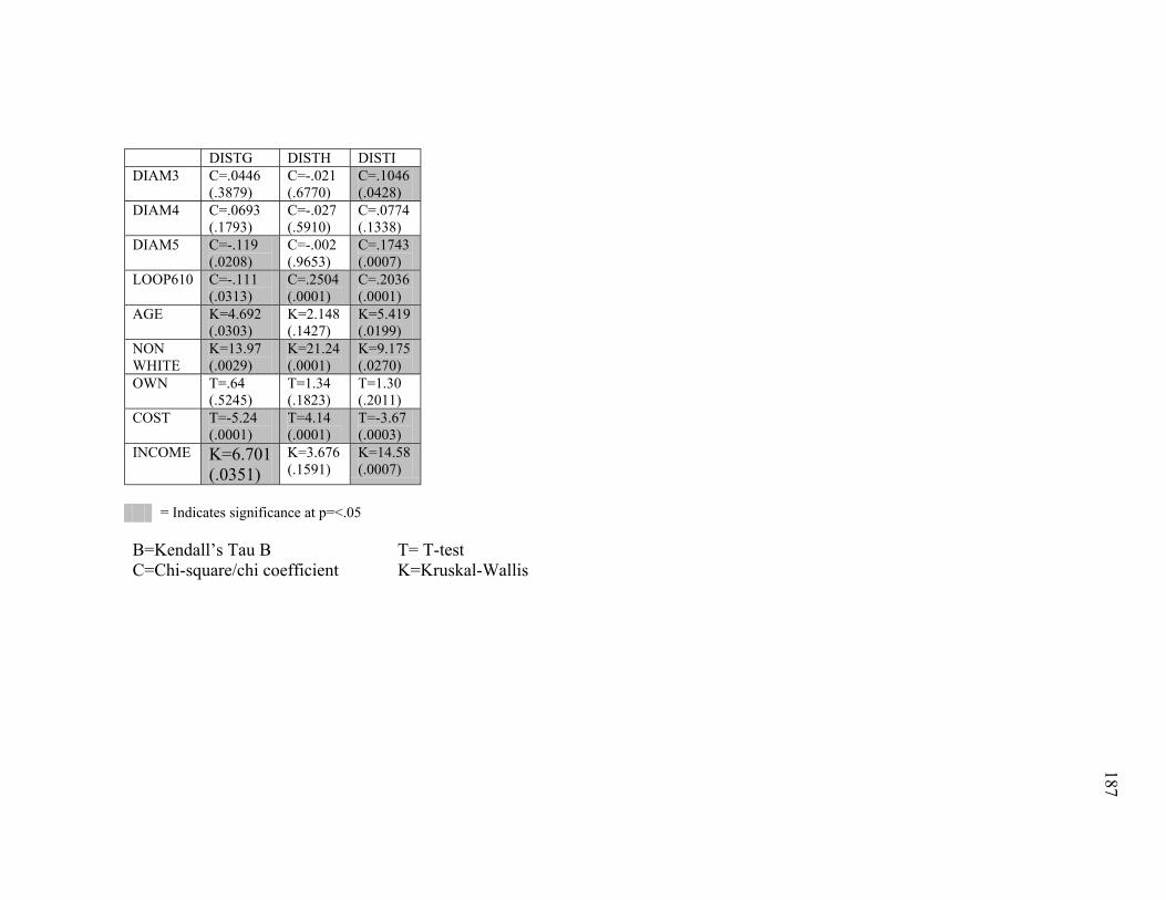
187

DISTG DISTH DISTI DIAM3 C=.0446

(.3879) C=-.021 (.6770)

C=.1046 (.0428)

DIAM4 C=.0693 (.1793)

C=-.027 (.5910)

C=.0774 (.1338)

DIAM5 C=-.119 (.0208)

C=-.002 (.9653)

C=.1743 (.0007)

LOOP610 C=-.111 (.0313)

C=.2504 (.0001)

C=.2036 (.0001)

AGE K=4.692 (.0303)

K=2.148 (.1427)

K=5.419 (.0199)

NON WHITE

K=13.97 (.0029)

K=21.24 (.0001)

K=9.175 (.0270)

OWN

T=.64 (.5245)

T=1.34 (.1823)

T=1.30 (.2011)

COST

T=-5.24 (.0001)

T=4.14 (.0001)

T=-3.67 (.0003)

INCOME

K=6.701 (.0351)

K=3.676 (.1591)

K=14.58 (.0007)

= Indicates significance at p=<.05 B=Kendall’s Tau B T= T-test C=Chi-square/chi coefficient K=Kruskal-Wallis

188

APPENDIX G: BIVARIATE ANALYSIS OF SEWER VARIBLES

NONWHITE OWN COST INCOME STABLE VOTE92 VOTE93 VOTE94 VOTE95 VOTE96 VOTE97 T_CASE K=.0032

(.9552) T=.29 (.7693)

T=1.18 (.2375)

K=.0330 (.8558)

K=6.298 (.0121)

K=.1370 (.7112)

K=.1520 (.6966)

K=.2905 (.5899)

K=.2905 (.5899)

K=.1025 (.7489)

K=.0536 (.8168)

T_COLL K=4.150 (.0416)

T=-.79 (.4321)

T=-2.36 (.0186)

K=3.117 (.0775)

K=.6066 (.4361)

K=2.384 (.1226)

K=2.691 (.1009)

K=3.489 (.0618)

K=3.489 (.0618)

K=3.772 (.0521)

K=2.872 (.0901)

T_FM K=.0621 (.8033)

T=-2.02 (.0436)

T=-.35 (.7272)

K=.1290 (.7194)

K=.8711 (.3507)

K=.1744 (.6763)

K=.0435 (.8347)

K=.0000 (.9945)

K=.0000 (.9945)

K=.0527 (.8184)

K=.0110 (.9163)

T_LATL K=2.913 (.0879)

T=1.04 (.2996)

T=-2.79 (.0055)

K=9.464 (.0021)

K=3.695 (.0546)

K=.5561 (.4558)

K=.9371 (.3330)

K=1.480 (.2237)

K=1.480 (.2237)

K=1.453 (.2279)

K=.7087 (.3999)

T_OF K=3.671 (.0553)

T=-.62 (.5366)

T=-1.32 (.1884)

K=1.105 (.2931)

K=4.064 (.0438)

K=.1846 (.6775)

K=.1972 (.6570)

K=.2753 (.5998)

K=.2753 (.5998)

K=.1427 (.7056)

K=.2206 (.6386)

T_SIPH K=.5538 (.4568)

T=-.85 (.3986)

T=.23 (.8199)

K=.7048 (.4012)

K=2.954 (.0856)

K=1.156 (.2821)

K=1.338 (.2474)

K=.8416 (.3589)

K=.8416 (.3589)

K=.7014 (.4023)

K=1.172 (.2790)

T-SLDG K=1.223 (.2687)

T=.41 (.6789)

T=-1.39 (.1665)

K=1.942 (.1634)

K=1.257 (.2622)

K=.0967 (.7558)

K=.1509 (.6977)

K=.0884 (.7662)

K=.0884 (.7662)

K=.1614 (.0398)

K=4.082 (.0433)

T_STUB K=.0016 (.9685)

T=-2.61 (.0093)

T=-.28 (.7773)

K=.7957 (.3724)

K=.0711 (.7898)

K=4.284 (.0385)

K=3.007 (.0829)

K=3.927 (.0475)

K=3.927 (.0475)

K=4.227 (.0980)

K=2.965 (.0851)

M_ABS K=4.070 (.0436)

T=.31 (.7555)

T=-1.56 (.1203)

K=3.888 (.0486)

K=.2360 (.6271)

K=.3510 (.5536)

K=.6639 (.4152)

K=1.514 (.2184)

K=1.514 (.2184)

K=1.556 (.2122)

K=1.389 (.2386)

M_CGMP K=.7593 (.3835)

T=1.10 (.2735)

T=.64 (.5222)

K=.3322 (.5644)

K=.1489 (.6996)

K=5.936 (.0148)

K=6.574 (.0103)

K=5.476 (.0193)

K=5.476 (.0193)

K=5.502 (.0190)

K=4.975 (.0257)

M_CI K=10.28 (.0013)

T=-1.42 (.1561)

T=-2.62 (.0092)

K=6.808 (.0091)

K=.0143 (.9050)

K=.6828 (.4086)

K=.7554 (.3848)

K=1.493 (.2217)

K=1.493 (.2217)

K=1.721 (.1895)

K=.8318 (.3618)

M_CLAY K=.0087 (.9259)

T=-1.11 (.2691)

T=-.21 (.8370)

K=1.119 (.2900)

K=.6884 (.4067)

K=.1056 (.7453)

K=.0194 (.8893)

K=.0086 (.9262)

K=.0086 (.9262)

K=.0613 (.8045)

K=.1283 (.7202)

M_CONC K=4.128 (.0422)

T=.03 (.9788)

T=-1.47 (.1416)

K=4.288 (.0384)

K=.0504 (.8223)

K=.0040 (.9497)

K=.2337 (.6288)

K=.0059 (.9387)

K=.0059 (.9387)

K=.0012 (.9720)

K=.0241 (.8766)

M_DI K=6.490 (.0108)

T=-.46 (.6483)

T=-3.09 (.0022)

K=3.293 (.0696)

K=6.504 (.0108)

K=.1746 (.6761)

K=.2248 (.6354)

K=.3439 (.5576)

K=.3439 (.5576)

K=.3290 (.5662)

K=.6837 (.4083)

M_MRC K=.0205 (.8861)

T=1.54 (.1241)

T=-.70 (.4827)

K=.6693 (.4133)

K=.3923 (.5311)

K=1.378 (.2403)

K=1.552 (.2128)

K=1.988 (.1585)

K=1.988 (.1585)

K=1.916 (.1662)

K=2.553 (.1101)

M_PVC

K=3.962 (.0465)

T=-.18 (.8606)

T=-2.50 (.0129)

K=10.76 (.0010)

K=.0711 (.7897)

K=.2439 (.6214)

K=.6389 (.4241)

K=.7051 (.4011)

K=.7051 (.4011)

K=.7804 (.3770)

K=1.045 (.3067)

= Indicates significance at p=<.05

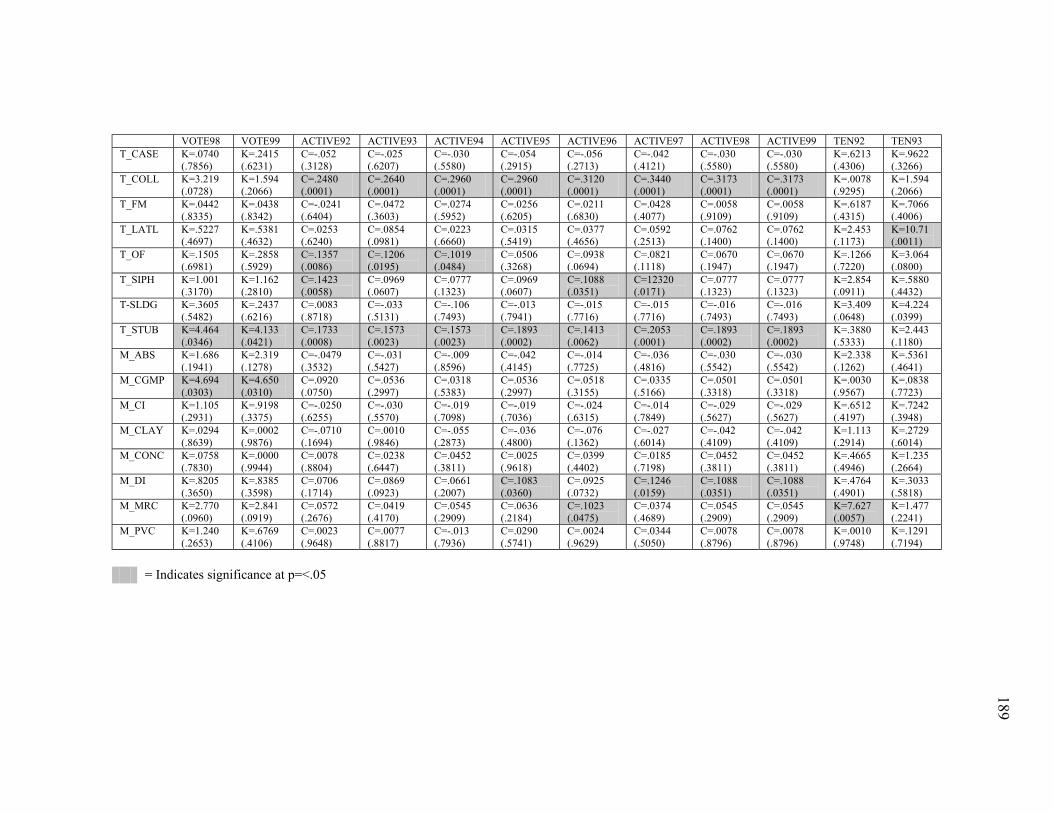
189

VOTE98 VOTE99 ACTIVE92 ACTIVE93 ACTIVE94 ACTIVE95 ACTIVE96 ACTIVE97 ACTIVE98 ACTIVE99 TEN92 TEN93 T_CASE

K=.0740 (.7856)

K=.2415 (.6231)

C=-.052 (.3128)

C=-.025 (.6207)

C=-.030 (.5580)

C=-.054 (.2915)

C=-.056 (.2713)

C=-.042 (.4121)

C=-.030 (.5580)

C=-.030 (.5580)

K=.6213 (.4306)

K=.9622 (.3266)

T_COLL K=3.219 (.0728)

K=1.594 (.2066)

C=.2480 (.0001)

C=.2640 (.0001)

C=.2960 (.0001)

C=.2960 (.0001)

C=.3120 (.0001)

C=.3440 (.0001)

C=.3173 (.0001)

C=.3173 (.0001)

K=.0078 (.9295)

K=1.594 (.2066)

T_FM K=.0442 (.8335)

K=.0438 (.8342)

C=-.0241 (.6404)

C=.0472 (.3603)

C=.0274 (.5952)

C=.0256 (.6205)

C=.0211 (.6830)

C=.0428 (.4077)

C=.0058 (.9109)

C=.0058 (.9109)

K=.6187 (.4315)

K=.7066 (.4006)

T_LATL K=.5227 (.4697)

K=.5381 (.4632)

C=.0253 (.6240)

C=.0854 (.0981)

C=.0223 (.6660)

C=.0315 (.5419)

C=.0377 (.4656)

C=.0592 (.2513)

C=.0762 (.1400)

C=.0762 (.1400)

K=2.453 (.1173)

K=10.71 (.0011)

T_OF K=.1505 (.6981)

K=.2858 (.5929)

C=.1357 (.0086)

C=.1206 (.0195)

C=.1019 (.0484)

C=.0506 (.3268)

C=.0938 (.0694)

C=.0821 (.1118)

C=.0670 (.1947)

C=.0670 (.1947)

K=.1266 (.7220)

K=3.064 (.0800)

T_SIPH K=1.001 (.3170)

K=1.162 (.2810)

C=.1423 (.0058)

C=.0969 (.0607)

C=.0777 (.1323)

C=.0969 (.0607)

C=.1088 (.0351)

C=12320 (.0171)

C=.0777 (.1323)

C=.0777 (.1323)

K=2.854 (.0911)

K=.5880 (.4432)

T-SLDG K=.3605 (.5482)

K=.2437 (.6216)

C=.0083 (.8718)

C=-.033 (.5131)

C=-.106 (.7493)

C=-.013 (.7941)

C=-.015 (.7716)

C=-.015 (.7716)

C=-.016 (.7493)

C=-.016 (.7493)

K=3.409 (.0648)

K=4.224 (.0399)

T_STUB K=4.464 (.0346)

K=4.133 (.0421)

C=.1733 (.0008)

C=.1573 (.0023)

C=.1573 (.0023)

C=.1893 (.0002)

C=.1413 (.0062)

C=.2053 (.0001)

C=.1893 (.0002)

C=.1893 (.0002)

K=.3880 (.5333)

K=2.443 (.1180)

M_ABS K=1.686 (.1941)

K=2.319 (.1278)

C=-.0479 (.3532)

C=-.031 (.5427)

C=-.009 (.8596)

C=-.042 (.4145)

C=-.014 (.7725)

C=-.036 (.4816)

C=-.030 (.5542)

C=-.030 (.5542)

K=2.338 (.1262)

K=.5361 (.4641)

M_CGMP K=4.694 (.0303)

K=4.650 (.0310)

C=.0920 (.0750)

C=.0536 (.2997)

C=.0318 (.5383)

C=.0536 (.2997)

C=.0518 (.3155)

C=.0335 (.5166)

C=.0501 (.3318)

C=.0501 (.3318)

K=.0030 (.9567)

K=.0838 (.7723)

M_CI K=1.105 (.2931)

K=.9198 (.3375)

C=-.0250 (.6255)

C=-.030 (.5570)

C=-.019 (.7098)

C=-.019 (.7036)

C=-.024 (.6315)

C=-.014 (.7849)

C=-.029 (.5627)

C=-.029 (.5627)

K=.6512 (.4197)

K=.7242 (.3948)

M_CLAY K=.0294 (.8639)

K=.0002 (.9876)

C=-.0710 (.1694)

C=.0010 (.9846)

C=-.055 (.2873)

C=-.036 (.4800)

C=-.076 (.1362)

C=-.027 (.6014)

C=-.042 (.4109)

C=-.042 (.4109)

K=1.113 (.2914)

K=.2729 (.6014)

M_CONC K=.0758 (.7830)

K=.0000 (.9944)

C=.0078 (.8804)

C=.0238 (.6447)

C=.0452 (.3811)

C=.0025 (.9618)

C=.0399 (.4402)

C=.0185 (.7198)

C=.0452 (.3811)

C=.0452 (.3811)

K=.4665 (.4946)

K=1.235 (.2664)

M_DI K=.8205 (.3650)

K=.8385 (.3598)

C=.0706 (.1714)

C=.0869 (.0923)

C=.0661 (.2007)

C=.1083 (.0360)

C=.0925 (.0732)

C=.1246 (.0159)

C=.1088 (.0351)

C=.1088 (.0351)

K=.4764 (.4901)

K=.3033 (.5818)

M_MRC K=2.770 (.0960)

K=2.841 (.0919)

C=.0572 (.2676)

C=.0419 (.4170)

C=.0545 (.2909)

C=.0636 (.2184)

C=.1023 (.0475)

C=.0374 (.4689)

C=.0545 (.2909)

C=.0545 (.2909)

K=7.627 (.0057)

K=1.477 (.2241)

M_PVC K=1.240 (.2653)

K=.6769 (.4106)

C=.0023 (.9648)

C=.0077 (.8817)

C=-.013 (.7936)

C=.0290 (.5741)

C=.0024 (.9629)

C=.0344 (.5050)

C=.0078 (.8796)

C=.0078 (.8796)

K=.0010 (.9748)

K=.1291 (.7194)

= Indicates significance at p=<.05

190

TEN94 TEN95 TEN96 TEN97 TEN98 TEN99 DISTA DISTB DISTC DISTD DISTE T_CASE

K=.9622 (.3266)

K=2.787 (.0950)

K=2.787 (.0950)

K=1.851 (.1736)

K=1.851 (.1736)

K=3.963 (.0465)

C=.0226 (.6622)

C=.1169 (.0236)

C=-.011 (.8184)

C=-.030 (.5548)

C=.1016 (.0490)

T_COLL K=1.594 (.2066)

K=1.142 (.2851)

K=1.142 (.2851)

K=3.145 (.0761)

K=3.145 (.0761)

K=4.486 (.0342)

C=.0093 (.8566)

C=-.087 (.0899)

C=-.050 (.3242)

C=-.014 (.7809)

C=.0914 (.0768)

T_FM K=.7066 (.4006)

K=.5227 (.4697)

K=.5227 (.4697)

K=3.201 (.0736)

K=3.201 (.0736)

K=3.985 (.0459)

C=.0208 (.6864)

C=.0257 (.6183)

C=-.079 (.1235)

C=.0704 (.1727)

C=.1309 (.0113)

T_LATL K=10.71 (.0011)

K=19.20 (.0001)

K=19.20 (.0001)

K=.0162 (.8987)

K=.0162 (.8987)

K=5.360 (.0206)

C=-.175 (.0007)

C=-.131 (.0111)

C=-.088 (.0866)

C=.059 (.2493)

C=-.079 (.1223)

T_OF K=3.064 (.0800)

K=4.424 (.0354)

K=4.424 (.0354)

K=1.563 (.2111)

K=1.563 (.2111)

K=4.903 (.0268)

C=-.052 (.3141)

C=-.123 (.0165)

C=.0199 (.7002)

C=.0248 (.6314)

C=.0445 (.3892)

T_SIPH K=.5880 (.4432)

K=4.273 (.0387)

K=4.273 (.0387)

K=.4240 (.5150)

K=.4240 (.5150)

K=.0672 (.7955)

C=.0877 (.0896)

C=-.081 (.1134)

C=.0788 (.1272)

C=.0291 (.5726)

C=-.071 (.1636)

T-SLDG K=4.224 (.0399)

K=3.681 (.0550)

K=3.681 (.0550)

K=.7720 (.3796)

K=.7720 (.3796)

K=2.498 (.1139)

C=-.038 (.4554)

C=.0457 (.3764)

C=.0333 (.5190)

C=-.084 (.1013)

C=.0107 (.8352)

T_STUB K=2.443 (.1180)

K=.0846 (.7712)

K=.0846 (.7712)

K=.9695 (.3248)

K=.9695 (.3248)

K=.2568 (.6124)

C=.0595 (.2489)

C=.0896 (.0827)

C=-.154 (.0028)

C=-.014 (.7809)

C=-.073 (.3007)

M_ABS K=.5361 (.4641)

K=.0731 (.7868)

K=.0731 (.7868)

K=.7097 (.3996)

K=.7097 (.3996)

K=.3479 (.5553)

C=.0383 (.4589)

C=-.122 (.0180)

C=.0113 (.8264)

C=.0643 (.2134)

C=.0815 (.1144)

M_CGMP K=.0838 (.7723)

K=.0281 (.8670)

K=.0281 (.8670)

K=.0215 (.8834)

K=.0215 (.8834)

K=.0303 (.8617)

C=-.029 (.5724)

C=.0170 (.7423)

C=-.021 (.6732)

C=.0304 (.5559)

C=.0199 (.6998)

M_CI K=.7242 (.3948)

K=.1204 (.7286)

K=.1204 (.7286)

K=1.612 (.2041)

K=1.612 (.2041)

K=.4897 (.4840)

C=.0730 (.1572)

C=-.037 (.2664)

C=-.107 (.0379)

C=-.014 (.7740)

C=.0130 (.8006)

M_CLAY K=.2729 (.6014)

K=5.849 (.0156)

K=5.849 (.0156)

K=3.701 (.0544)

K=3.701 (.0544)

K=7.511 (.0061)

C=-.025 (.6164)

C=.0136 (.7926)

C=-.032 (.5308)

C=-.044 (.3856)

C=.1984 (.0001)

M_CONC K=1.235 (.2664)

K=.4112 (.5214)

K=.4112 (.5214)

K=.0763 (.7823)

K=.0763 (.7823)

K=.0411 (.8394)

C=.0447 (.3864)

C=-.037 (.4708)

C=.0373 (.4699)

C=.0039 (.9504)

C=-.087 (.0887)

M_DI K=.3033 (.5818)

K=.3274 (.5672)

K=.3274 (.5672)

K=2.928 (.0871)

K=2.928 (.0871)

K=3.336 (.0678)

C=.0266 (.6060)

C=-.069 (.1783)

C=.0175 (.7343)

C=.0204 (.6934)

C=4.307 (.0380)

M_MRC K=1.477 (.2241)

K=.0214 (.8836)

K=.0214 (.8836)

K=1.799 (.1798)

K=1.799 (.1798)

K=1.078 (.2991)

C=.0528 (.3062)

C=-.123 (.0169)

C=.0149 (.9028)

C=.1310 (.0112)

C=-.036 (.4822)

M-PVC K=.1291 (.7194)

K=1.897 (.1684)

K=1.897 (.1684)

K=.9487 (.3300)

K=.9487 (.3300)

K=2.830 (.0925)

C=-.037 (.4731)

C=-.035 (.4951)

C=-.047 (.3604)

C=.0362 (.4831)

C=.094 (.0662)

= Indicates significance at p=<.05

191

DISTF DISTG DISTH DISTI T_CASE

C=-.052 (.3099)

C=-.102 (.0465)

C=-.101 (.0504)

C=.1052 (.0417)

T_COLL C=.0563 (.2760)

C=.0970 (.0603)

C=-.142 (.0059)

C=.0873 (.0909)

T_FM C=-.056 (.2733)

C=.0511 (.3225)

C=-.103 (.0459)

C=.0959 (.0633)

T_LATL C=-.175 (.0007)

C=-.064 (.2131)

C=.2825 (.0001)

C=.2958 (.0001)

T_OF C=-.094 (.0688)

C=.0640 (.2154)

C=-.023 (.6491)

C=.1331 (.0099)

T_SIPH C=.1256 (.0150)

C=-.081 (.1164)

C=-.022 (.6675)

C=-.037 (.4675)

T-SLDG C=-.072 (.1597)

C=.0029 (.9548)

C=-.117 (.0226)

C=.2305 (.0001)

T_STUB C=-.166 (.0013)

C=.0096 (.8518)

C=.0991 (.0550)

C=.0700 (.1751)

M_ABS C=.1216 (.0186)

C=.2299 (.0001)

C=-.230 (.0001)

C=-.127 (.0136)

M_CGMP C=-.005 (.9136)

C=.1009 (.0507)

C=-.081 (.1159)

C=-.021 (.6732)

M_CI C=.1993 (.0001)

C=.1972 (.0001)

C=-.232 (.0001)

C=.0138 (.7888)

M_CLAY C=-.091 (.0761)

C=-.089 (.0842)

C=-.021 (.6817)

C=.0890 (.0848)

M_CONC C=.0308 (.8606)

C=.1163 (.0243)

C=-.094 (.0667)

C=.0373 (.4699)

M_DI C=.0464 (.3694)

C=.1135 (.0280)

C=-.2129 (.0001)

C=.002 (.9964)

M_MRC C=.0774 (.1340)

C=.0138 (.7900)

C=-.044 (.3937)

C=-.063 (.2167)

M-PVC C=.0145 (.7785)

C=.1181 (.0222)

C=-.137 (.0077)

C=.0219 (.6717)

= Indicates significance at p=<.05

192

NONWHITE OWN COST INCOME STABLE VOTE92 VOTE93 VOTE94 VOTE95 VOTE96 VOTE97 M_RCP K=2.103

(.1469) T=.58 (.5630)

T=-1.24 (.2154)

K=1.250 (.2634)

K=.6741 (.4116)

K=2.978 (.0844)

K=3.319 (.0865)

K=3.436 (.0638)

K=3.436 (.0638)

K=3.662 (.0556)

K=1.982 (.1591)

M_STL K=.0056 (.9404)

T=-.29 (.7722)

T=.45 (.6529)

K=.1304 (.7180)

K=.7411 (.3893)

K=.1293 (.7192)

K=.0143 (.9047)

K=.0030 (.9560)

K=.0030 (.9560)

K=.1360 (.7123)

K=.1179 (.7313)

DIAM1 K=1.326 (.2494)

T=-.32 (.7457)

T=-1.98 (.0482)

K=4.528 (.0333)

K=2.621 (.1054)

K=.5391 (.4628)

K=.3329 (.5640)

K=.5058 (.4770)

K=.5058 (.4770)

K=.2214 (.6380)

K=.5046 (.4775)

DIAM2 K=.0337 (.8543)

T=-1.03 (.3058)

T=.71 (.4751)

K=.2633 (.6079)

K=1.777 (.1825)

K=9.749 (.0018)

K=10.98 (.0009)

K=11.41 (.0007)

K=11.41 (.0007)

K=12.24 (.0005)

K=10.68 (.0011)

DIAM3 K=4.027 (.0448)

T=-.87 (.3834)

T=-1.72 (.0868)

K=.8630 (.3529)

K=.6741 (.4116)

K=.3836 (.5357)

K=.1919 (.6613)

K=.0625 (.8026)

K=.0625 (.8026)

K=.0699 (.7914)

K=.3545 (.5516)

DIAM4 K=7.550 (.0060)

T=-.47 (.6396)

T=-3.08 (.0022)

K=10.56 (.0012)

K=3.890 (.0486)

K=1.209 (.2715)

K=1.300 (.2541)

K=1.312 (.2520)

K=1.312 (.2520)

K=1.956 (.1619)

K=1.752 (.1855)

LOOP610 K=5.331 (.0209)

T=.51 (.6117)

T=-4.60 (.0001)

K=17.10 (.0001)

K=.6785 (.4101)

K=5.982 (.0145)

K=6.409 (.0114)

K=6.169 (.0130)

K=6.169 (.0130)

K=6.053 (.0139)

K=4.824 (.0281)

AGE B=.1773 (.0000)

B=.0190 (.5878)

B=-.324 (.0001)

B=-.340 (.0001)

B=-.021 (.6164)

B=.0860 (.0664)

B=.0283 (.7681)

B=.0449 (.6394)

B=.0449 (.6394)

B=.0370 (.6999)

B=.0310 (.7480)

MIN

B=-.041 (.3740)

B=.0310 (.7690)

B=-.003 (.9751)

B=-.038 (.7130)

B=-.038 (.7130)

B=-.046 (.6573)

B=-.050 (.6371)

OWN

B=-.046 (.2698)

B=.1362 (.1538)

B=.1348 (.1576)

B=.1465 (.1243)

B=.1465 (.1243)

B=.1333 (.1626)

B=.1284 (.1806)

COST

B=.0329 (.4522)

B=-.053 (.5902)

B=-.026 (.7902)

B=-.000 (.9952)

B=-.000 (.9952)

B=.0065 (.9569)

B=-.029 (.7653)

INCOME

B=-.007 (.8810)

B=-.053 (.6374)

B=-.010 (.9272)

B=-.019 (.8662)

B=-.019 (.8662)

B=.0063 (.9551)

B=-.003 (.9774)

= Indicates significance at p=<.05

193

VOTE98 VOTE99 ACTIVE92 ACTIVE93 ACTIVE94 ACTIVE95 ACTIVE96 ACTIVE97 ACTIVE98 ACTIVE99 TEN92 TEN93 M_RCP K=2.249

(.1336) K=2.826 (.0927)

C=.0129 (.8020)

C=.0077 (.8817)

C=-.002 (.9561)

C=.0077 (.8817)

C=.0238 (.6455)

C=.0344 (.5050)

C=.0185 (.7203)

C=.0185 (.7203)

K=.0423 (.8371)

K=.3847 (.5351)

M_STL K=.1449 (.7034)

K=.0622 (.8030)

C=-.0072 (.8890)

C=.0182 (.7251)

C=-.014 (.7764)

C=-.009 (.8511)

C=-.040 (.4382)

C=.0017 (.9730)

C=-.014 (.7764)

C=-.014 (.7764)

K=.0908 (.7632)

K=1.183 (.2766)

DIAM1 K=.6124 (.4339)

K=.6291 (.4277)

C=-.0130 (.8010)

C=.0510 (.3237)

C=.0095 (.8543)

C=.0058 (.9108)

C=.0020 (.9693)

C=-.009 (.8570)

C=.0095 (.8543)

C=.0095 (.8543)

K=.9684 (.3251)

K=.3892 (.5327)

DIAM2 K=10.08 (.0015)

K=10.32 (.0013)

C=.2319 (.0001)

C=.2265 (.0001)

C=.2586 (.0001)

C=.2586 (.0001)

C=.2426 (.0001)

C=.3066 (.0001)

C=.2693 (.0001)

C=.2693 (.0001)

K=.0436 (.8347)

K=1.595 (.2066)

DIAM3 K=.2205 (.6386)

K=.0438 (.8342)

C=.0877 (.0896)

C=.0610 (.2372)

C=.0505 (.3281)

C=.0504 (.3294)

C=.0558 (.2802)

C=.0771 (.1354)

C=.0612 (.2362)

C=.0612 (.2362)

K=2.116 (.1458)

K=.9214 (.3371)

DIAM4 K=1.453 (.2280)

K=1.423 (.2329)

C=.1566 (.0024)

C=.1301 (.0118)

C=.1624 (.0017)

C=.1407 (.0064)

C=.1782 (.0006)

C=.1676 (.0012)

C=.1624 (.0017)

C=.1624 (.0017)

K=.0006 (.9798)

K=.1589 (.6901)

LOOP610 K=5.093 (.0240)

K=4.163 (.0413)

C=.0310 (.5484)

C=-.030 (.0602)

C=.0784 (.1290)

C=-.056 (.2713)

C=.0093 (.0702)

C=.0935 (.0702)

C=.1132 (.0281)

C=.1132 (.0284)

K=.0834 (.7728)

K=11.13 (.0008)

AGE B=.0316 (.7433)

B=-.005 (.9519)

T=-1.39 (.1664)

T=-2.02 (.0441)

T=-3.13 (.0019)

T=-3.01 (.0028)

T=-3.05 (.0024)

T=-2.75 (.0062)

T=-3.22 (.0014)

T=-3.22 (.0014)

B=-.046 (.2862)

B=-.041 (.3232)

NON WHITE

B=-.036 (.7292)

B=-.061 (.5602)

K=6.218 (.1014)

K=3.142 (.3702)

K=5.636 (.1307)

K=3.416 (.3317)

K=2.529 (.4700)

K=1.724 (.6314)

K=3.289 (.3490)

K=3.289 (.3490)

B=.0433 (.3600)

-.1413 (.0020)

OWN

B=.1209 (.2074)

B=.1269 (.1844)

T=-.58 (.5616)

T=-.39 (.6987)

T=-.69 (.4890)

T=-.67 (.5028)

T=-.32 (.7494)

T=-.02 (.9814)

T=-.85 (.3933)

T=-.85 (.3933)

B=-.021 (.6074)

B=-.032 (.4248)

COST

B=.0145 (.8837)

B=.0414 (.6756)

T=-1.59 (.1137)

T=-1.22 (.2222)

T=-1.03 (.3201)

T=-.54 (.5883)

T=-.83 (.4061)

T=.08 (.9333)

T=-.83 (.4093)

T=-.83 (.4093)

B=-.014 (.7460)

B=.1334 (.0017)

INCOME

B=-.018 (.8705)

B=.018 (.8712)

K=1.235 (.5390)

K=.8920 (.6402)

K=.4343 (.8048)

K=.0898 (.9561)

K=.1412 (.9318)

K=.4574 (.7956)

K=.2898 (.8651)

K=.2898 (.8651)

B=.0463 (.3538)

B=.0907 (.0605)

= Indicates significance at p=<.05

194

TEN94 TEN95 TEN96 TEN97 TEN98 TEN99 DISTA DISTB DISTC DISTD DISTE M_RCP K=.3847

(.5351) K=.0134 (.9080)

K=.0134 (.9080)

K=.9487 (.3300)

K=.9487 (.3300)

K=2.830 (.0925)

C=.0036 (.9449)

C=.0292 (.5716)

C=-.099 (.0551)

C=-.010 (.8452)

C=.0768 (.1371)

M_STL K=1.183 (.2766)

K=2.797 (.0944)

K=2.797 (.0944)

K=.0734 (.7864)

K=.0734 (.7864)

K=.1483 (.7001)

C=.0288 (.5773)

C=.0127 (.8062)

C=-.048 (.0484)

C=-.046 (.3716)

C=.1788 (.0005)

DIAM1 K=.3892 (.5327)

K=1.183 (.2766)

K=1.183 (.2766)

K=.0019 (.9653)

K=.0019 (.9653)

K=.4862 (.4856)

C=-.061 (.2368)

C=.0035 (.9452)

C=-.026 (.6100)

C=-.077 (.8813)

C=.094 (.0688)

DIAM2 K=1.595 (.2066)

K=.5784 (.4469)

K=.5784 (.4469)

K=2.565 (.1092)

K=2.565 (.1092)

K=2.796 (.0945)

C=.028 (.5875)

C=.0272 (.5985)

C=-.118 (.0221)

C=-.012 (.8129)

C=.0569 (.2703)

DIAM3 K=.9214 (.3371)

K=.1304 (.7180)

K=.1304 (.7180)

K=3.847 (.0498)

K=3.874 (.0498)

K=3.592 (.0581)

C=.0466 (.3663)

C=-.131 (.0107)

C=-.081 (.1132)

C=.0517 (.3172)

C=.0768 (.1371)

DIAM4 K=.1589 (.6901)

K=1.446 (.2292)

K=1.446 (.2292)

K=.0304 (.8615)

K=.0304 (.8615)

K=.3340 (.5633)

C=-.064 (.2096)

C=-.061 (.2344)

C=-.024 (.6362)

C=.058 (.2606)

C=-.008 (.8685)

LOOP610 K=11.13 (.0008)

K=17.72 (.0001)

K=17.72 (.0001)

K=.8139 (.3670)

K=.8139 (.3670)

K=1.306 (.1790)

C=-.201 (.0001)

C=-.057 (.2649)

C=-.003 (.9536)

C=.2045 (.0001)

C=-.215 (.0001)

AGE B=-.041 (.3232)

B=.2518 (.0001)

B=.2518 (.0001)

B=.0553 (.1838)

B=.0553 (.1838)

B=-.172 (.0001)

K=17.00 (.0001)

K=2.684 (.1013)

K=1.343 (.2465)

K=6.049 (.0139)

K=15.32 (.0001)

NON WHITE

B=-.143 (.0020)

B=.1739 (.0001)

B=.1739 (.0001)

B=.1118 (.0140)

B=.1118 (.0140)

B=-.165 (.0003)

K=4.336 (.2273)

K=21.43 (.0001)

K=2.075 (.5568)

K=6.448 (.0917)

K=3.815 (.2821)

OWN

B=-.032 (.4248)

B=.0345 (.3981)

B=.0345 (.3981)

B=-.032 (.4328)

B=-.032 (.4328)

B=.0085 (.8353)

T=-1.19 (.2344)

T=-1.23 (.2183)

T=1.01 (.3116)

T=.57 (.5687)

T=-1.53 (.1270)

COST

B=.1334 (.0017)

B=-.224 (.0001)

B=-.224 (.0001)

B=-.073 (.0809)

B=-.073 (.0809)

B=.1728 (.0001)

T=3.15 (.0018)

T=4.72 (.0001)

T=-.31 (.7589)

T=-2.77 (.0060)

T=-.37 (.7144)

INCOME

B=.0907 (.0605)

B=-.204 (.0001)

B=-.204 (.0001)

B=-.033 (.4920)

B=-.033 (.4920)

B=.1331 (.0057)

K=11.45 (.0033)

K=15.72 (.0004)

K=.4153 (.8125)

K=3.004 (.2226)

K=7.060 (.0293)

= Indicates significance at p=<.05

195

DISTF DISTG DISTH DISTI M_RCP C=.1034

(.0452) C=.1181 (.0222)

C=-.137 (.0077)

C=-.030 (.5619)

M_STL C=-.061 (.2360)

C=-.067 (.1900)

C=-.075 (.1448)

C=.0869 (.0924)

DIAM1 C=.0064 (.9014)

C=.0905 (.0795)

C=-.087 (.0904)

C=.0102 (.8428)

DIAM2 C=-.053 (.3000)

C=-.049 (.3383)

C=-.049 (.3383)

C=.0719 (.1640)

DIAM3 C=.1257 (.0149)

C=.1880 (.0003)

C=-.198 (.0001)

C=-.012 (.8062)

DIAM4 C=.1076 (.0372)

C=.0537 (.2984)

C=-.055 (.2807)

C=.0274 (.5954)

LOOP610 C=-.168 (.0011)

C=-.111 (.0313)

C=.2504 (.0001)

C=.2036 (.0001)

AGE K=.0325 (.8569)

K=4.692 (.0303)

K=2.148 (.1427)

K=5.419 (.0199)

NON WHITE

K=19.95 (.0002)

K=13.97 (.0029)

K=21.24 (.0001)

K=9.175 (.0270)

OWN

T=2.78 (.0096)

T=.64 (.5245)

T=1.34 (.1823)

T=1.30 (.2011)

COST

T=.27 (.7891)

T=-5.24 (.0001)

T=4.14 (.0001)

T=-3.67 (.0003)

INCOME

K=1.329 (.5145)

K=6.701 (.0351)

K=3.676 (.1591)

K=14.58 (.0007)

= Indicates significance at p=<.05 B=Kendall’s Tau B T= T-test C=Chi-square/Phi coefficient K=Kruskal-Wallis

196

VITA

SHERI LASHEL SMITH 7817 E. Gregory Blvd.

Kansas City, Missouri 64133 EDUCATION Doctor of Philosophy, Urban and Regional Science May 2002 Department of Landscape Architecture and Urban Planning Texas A&M University, College Station, Texas Dissertation Topic: Testing the influence of socio, political and technical factors on the selection of capital improvement projects. Master of Urban and Regional Planning August 1988 Department of Urban and Regional Planning University of Illinois, Champaign-Urbana, Illinois Masters Project: Creation of comprehensive plan for Vandalia, Illinois Bachelor of Arts in Sociology May 1986 George Washington University, Washington, DC. Minor: Economics EXPERIENCE Summer Enhancement Program for Teachers. Special program within the School of Engineering at Texas A&M University. Consultant Summer 1999, 2000, 2001 Indian Nation Council of Governments (INCOG), Tulsa, Oklahoma Community Development Planner April 1994 - December 1996 Community Planner April 1993 - March 1994 Project Get Together/PGT Housing, Tulsa, Oklahoma Consultant April 1994 - December 1996 Housing Development Coordinator August 1993 - March 1994 Neighborhood Housing Services (NHS), Chicago, Illinois Special Project Coordinator July 1992 - January 1993 Neighborhood Director July 1990 - June 1992 Neighborhood Manager August 1988 - June 1990