Managing Expectations in the New KeynesianModel*

Robert G. King Yang K. Lu

First draft: Feb 2019. This draft: August 2021

Abstract

This paper uses a monetary regime shift model to describe the main features of

inflation and real activity in the U.S. between the late 1960s and the mid 2000s. Our

model features occasional, observable changes in regime, a forward-looking New Key-

nesian Phillips curve, and Bayesian learning by the private sector about the type of

policymaker that is in place. When a regime change occurs, the new policymaker can

be of one of two types: it is either endowed with the ability to commit to its future

policies (a committed type) or not (an opportunistic type). Being able to commit or

not, the policymaker in place chooses inflation policies optimally, taking into account

the learning and rational expectation of the private sector. We show that the equilib-

rium can be obtained as a solution to a recursive optimization of the committed type

in which the actions of the opportunistic type are subject to an incentive compatibility

constraint. Numerical exercises using a standard calibration reveal that our model can

capture the rise, fall, and relative stabilization of US inflation between 1970 and 2005.

Keywords: time inconsistency, reputation game, optimal monetary policy, forward-

looking expectations

JEL classifications: E52, D82, D83.

*We would like to thank the audience at various conferences and seminars for helpful comments anddiscussions. All errors are ours. We acknowledge the financial support from the RGC of HKSAR (GRFHKUST-16504317).

Boston University and NBER. Email: 〈rking@bu.edu〉Corresponding author, Hong Kong University of Science and Technology. Email: 〈yanglu@ust.hk〉

“In reality, however, the anchoring of inflation expectations has been a hard-won

achievement of monetary policy over the past few decades, and we should not

take this stability for granted. [...] a policy of achieving “temporarily” higher in-

flation over the medium term would run the risk of altering inflation expectations

beyond the horizon that is desirable. Were that to happen, the costs of bringing

expectations back to their current anchored state might be quite high.”

(Donald L. Kohn, “Monetary Policy Research and the Financial Crisis: Strengths

and Shortcomings”, October 9, 2009)

1 Introduction

Figure 1 plots the one-quarter-ahead inflation forecast errors in the U.S. from 1969 to 2005.1 If

we compute the 8-quarter average of the forecast error and plot it using the black dashed line,

it reveals a turning point around 1980 when the average inflation forecast error turned from

persistently positive to persistently negative. This pattern of persistently nonzero forecast

errors has been used in the literature as evidence for the private sector’s learning with some

misspecified model of the economy.2

We take a different approach in this paper and argue that it is due to the private sector’s

learning about the type of the policymaker in place. Before 1980, the policymaker in the

U.S. was a type that could not commit. After 1980, the policymaker changed to a committed

type that carried out promised inflation plans. The private sector did not observe the type of

the policymaker and had to learn which type it was facing from the past inflation experience.

Turning these simple ideas into macroeconomic time series is the main activity of our research.

We show a basic model of shifting policy regimes can capture the rise, fall, and relative

stabilization of US inflation between the late 1960s and the mid 2000s. The key ingredients

are a forward-looking New Keynesian Phillips curve, policymakers that can or cannot commit,

Bayesian learning by the private sector about policymaker type, and a committed type that

manages expectations with an eye to building reputation.

When a regime change occurs, the new policymaker may be a commitment type endowed

with the ability to subsequently carry out its future inflation policies. If not, as in the

standard Barro-Gordon framework, it simply chooses inflation taking as given the behavior

of expectations (it is myopic, but we call it an opportunistic type). With a policymaker that

can’t commit, our model would – under full information rational expectations – exhibit an

immediate jump to a high inflation rate until another regime change.

But in our model with learning, the rise in inflation can be very gradual, transiting from a

small amount of intrinsic inflation bias (a policymaker’s choice with well-anchored expected

inflation) to a large ultimate bias of 8% or more (at the Nash equilibrium in the terminology of

1The data is from the Survey of Professional Forecasters obtained from the website of the Federal ReserveBank of Philadelphia.

2We thank Donghai Zhang for pointing us to this observation.

1

Figure 1: Forecast error of inflation

The GDP inflation rate, πt, and the Survey of Professional Forecasters’s median inflation forecast

rate made one quarter earlier, ft|t−1, rise and fall together over 1968Q4 through 2005Q4. Inflation

is notoriously difficult to forecast so that the forecasting error, πt − ft|t−1, is volatile, although it

averages close to zero over the sample period. The errors display serial correlation – lengthy runs

of positive and negative forecasting values – that are highlighted by an 8 quarter moving average.

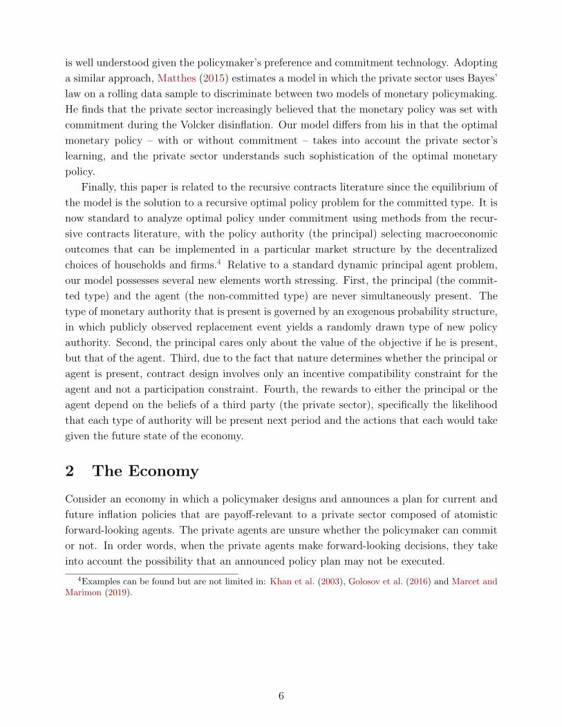
The one quarter ahead forecast ft+1|t and the three quarter ahead forecast ft+3|t rise and fall

together. The SPF spread ft+3|t − ft+1|t, which will play an important role in the paper, also

displays sustained intervals of high or low values. All variables are continuously compounded

annualized rates of change. Additional detail on macroeconomic data and the SPF constructions

are provided in Appendix XX.

Figure 2: SPF and SPF Spread

2

Sargent [1999] and others). The key mechanism is the positive feedback between the choices

of a policymaker that can’t commit and expectations. The process of transition to Nash

equilibrium is complicated by learning, in a manner that is revealing about some particular

stages of “ the Great Inflation.”

Another important modeling challenge is to describe the behavior of the committed type

of policymaker. It has to manage inflation and inflation expectations knowing that private

agents have concerns that the opportunistic type is in charge. The private sector’s assessment

of the likelihood of there being a committed type – its reputation – becomes a key state

variable which evolves like a capital good. We use a recursive approach to policy design

to determine optimal committed policymaker’s choice within a Markovian equilibrium with

private sector learning and prospective regime change.

In our model, the optimal policies of the committed type and the opportunistic type

determine the policy difference between two “regimes’ in the sense of the “Markov switching”

models pioneered by Hamilton [1989]. But relative to the basic “Markov switching’ model,

the policy difference varies endogenously with the private sector’s belief about policymaker

type. In particular, the policy difference is small when the private sector believes that the

committed type most likely is in place; and is larger when it thinks otherwise. The private

sector’s belief, in turn, is determined by past policy differences via Bayesian learning.

We show that the interplay of optimal policy choices by each type within a regime and

private sector’s beliefs resolves a dilemma for mechanical Markov switching models: we can

making the learning relevant while matching the large inflation swings during the period of

the Great inflation and the Volcker disinflation.

For example, at the start of a Great Inflation initiated by a switch to the opportunistic

type, rising actual inflation can have relatively minor effects on expected inflation, since the

private sector believes that the committed type most likely is in place and expects future

anti-inflation policies. Further, the opportunistic type opts not to increase inflation much

because its intrinsic bias is small and expectations are low and stable. In turn, this makes

for slow learning.

Contemporary observers and later analysts have described substantial “price Shocks’ dur-

ing the 1970s highlighting changes in oil and energy, food, imported goods and so on. Our

NK optimal policy framework contains such ultimately transitory shocks, but our theoretical

analysis shows that a positive shock leads to a larger policy difference, leading to a decline

in reputation and higher inflation after the shock’s direct effects have worn away.

If a regime switch occurs in early 1980s, a transition to a committed type that has weak

initial reputation can lead to a Volcker-style disinflation. Forward-looking NK inflation dy-

namics play an important role in such situations. For example, both the full-commitment

solution and a loose-commitment solution exhibit “start-up’ inflation with initial high but

declining inflation after a regime switch but are associated with a real boom. Matters are

quite different in our model when there is a new committed policymaker that has weak initial

3

reputation. This policymaker sees high initial expected inflation because the private sector

believes it is likely that is facing an opportunistic type. An optimal action for the new com-

mitted policymaker must balance accommodating high expected inflation and differentiating

itself from an opportunistic inflation policy. Hence, tough inflation actions lead to a decline

in real activity rather than a boom. Over time, the private sector learns and puts less weight

on an opportunistic type being in place. So the expected inflation declines, resulting in a

lower perceived optimal opportunistic policy by the private sector, which further reduces the

expected inflation, and hence the optimal committed inflation policies. Along the disinfla-

tion transition path, there is an initial stage of large output loss as the cost of signaling by

the committed type. As its reputation improves over time, the signaling incentive of the

committed type weakens and learning becomes more gradual.

Lastly, we use a quantitative exercise to demonstrate the quantitative importance of the

key mechanism in our model. In particular, we extract information from multi-step inflation

forecasts in SPF to construct measures of latent state variables – namely reputation and price

shocks – in our model. The idea is that a near-term forecast is more sensitive to temporary

price shocks, while a longer-term forecast better reflects reputation. Figure 2 couples SPF

forecasts made at a particular date using two different horizons – one-quarter-ahead (SPF1Q)

and three-quarter-ahead (SPF3Q). It is clear that these series rise and fall together. Figure

2 also plot the SPF Spread defined as SPF1Q-SPF3Q. This construction highlights intervals

when the forecasters thought that there were important inflation developments that would

ultimately prove transitory. The extracted reputation states and price shocks, together with

a set of specified regime switch dates (we use the initial quarter of Fed chairmen 1970-

1987), allow us to compute model time series of committed policy and opportunistic policy.

Although not designed to do so, we find the U.S. inflation between 1970 and 2005 is tracked by

the constructed opportunistic policies before 1981 and by the constructed committed policies

afterwards. Moreover, using a counterfactual exercise, we show the success of our model in

matching the U.S. inflation can be attributed to time-varying reputation, which highlights

the quantitative importance of the dynamic interplay between private sector’s belief and the

optimal policy choices.

Our model is deliberately stark. But it yields results that have surprised us and others.

We believe its success in matching the U.S. time series means that there is great empirical

promise, rather than an evident deficiency, in studying models with policy regimes of varying

commitment capability and private sector learning.

The organization of the paper is as follows. In section 2, we describe our model economy.

In section 3, we detail the perfect Bayesian equilibrium that we envision, which features ran-

dom publicly observable replacements of policymakers of a type unknown to private agents,

learning within a regime, and consistent beliefs about prospective regime change. In section

4, we highlight the more complicated decision problem of the committed type, but show that

it fits neatly into a recursive equilibrium and we briefly discuss computational issues. In sec-

4

tion 5, we provide detailed information about our calibrated strategy and how comparative

dynamics arising from variations in initial conditions or shocks can qualitatively replicates

important features of the Great Inflation and the Volcker Disinflation. In section 6, having

extracted model states – including reputation – we put the model to work in interpreting US

macroeconomic time series. Section 7 provides some concluding remarks.

Related literature This paper is closely related to the reputation literature on monetary

policy. The early representative examples of this literature are Barro (1986), Backus and

Driffill (1985a) and Backus and Driffill (1985b). They show that reputational force can disci-

pline a discretionary policymaker to behave like a committed type, who mechanically adopts

an exogenously given policy rule. Other papers in this literature put more emphasis on the

optimal behavior of the committed policymaker. Cukierman and Liviatan (1991) and King

et al. (2008) study how reputation concerns change the optimal committed monetary pol-

icy in a setting with the Lucas-Barro-Gordon Phillips curve. Hansen and McMahon (2016)

and Xandri (2017) show the importance of signaling in monetary policy decisions, in which

the ”good” type of policymaker has a binary choice of signals. Dovis and Kirpalani (2019)

study the optimal policy chosen by the rule designer when there is uncertainty about the

type of policymaker, in settings that do not feature forward-looking expectations. The most

related paper is Lu et al. (2016), which studies optimal reputation building by the committed

policymaker in a NK model with the non-committed policymaker mechanically following a

given policy rule. Lu et al. (2016) finds that reputation building incentives make the com-

mitted policymaker less prone to simulate output with initially high but declining inflation

and its inflation responses less accommodating to energy-price shocks. In the current paper,

we treat both types of policymakers (committed or non-committed) as strategic players and

solve for their optimal inflation policies in a single recursive optimization problem. We find

that taking into account the optimal responses of a non-committed policymaker significantly

changes the reputation building incentives of the committed policymaker, making the effect

of reputation on optimal committed policy highly nonlinear.

In this paper, the rich dynamics of reputation is governed by the private sector’s learning

about the type of the policy authority in place. Our model thus belongs to the vast learning

literature on monetary policy,3 which is well known to be more consistent with basic facts

about measured expectations and forecasting errors than the standard rational expectation

(RE) approach. Most papers in the literature assume that the agents learn using a misspec-

ified model of the economy. Our approach differs in that our private sector possesses prefect

knowledge about the economic model (i.e., the mapping from the states to the policies), yet

incomplete information of the type of policy authority. These two approaches are comple-

mentary in capturing different uncertainty regarding the fundamentals of the economy. Our

approach is more appropriate for studying an economy in which the optimal monetary policy

3See Evans and Honkapohja (2003), Evans and Honkapohja (2008), Woodford (2013) and Eusepi andPreston (2018) for the surveys of this literature.

5

is well understood given the policymaker’s preference and commitment technology. Adopting

a similar approach, Matthes (2015) estimates a model in which the private sector uses Bayes’

law on a rolling data sample to discriminate between two models of monetary policymaking.

He finds that the private sector increasingly believed that the monetary policy was set with

commitment during the Volcker disinflation. Our model differs from his in that the optimal

monetary policy – with or without commitment – takes into account the private sector’s

learning, and the private sector understands such sophistication of the optimal monetary

policy.

Finally, this paper is related to the recursive contracts literature since the equilibrium of

the model is the solution to a recursive optimal policy problem for the committed type. It is

now standard to analyze optimal policy under commitment using methods from the recur-

sive contracts literature, with the policy authority (the principal) selecting macroeconomic

outcomes that can be implemented in a particular market structure by the decentralized

choices of households and firms.4 Relative to a standard dynamic principal agent problem,

our model possesses several new elements worth stressing. First, the principal (the commit-

ted type) and the agent (the non-committed type) are never simultaneously present. The

type of monetary authority that is present is governed by an exogenous probability structure,

in which publicly observed replacement event yields a randomly drawn type of new policy

authority. Second, the principal cares only about the value of the objective if he is present,

but that of the agent. Third, due to the fact that nature determines whether the principal or

agent is present, contract design involves only an incentive compatibility constraint for the

agent and not a participation constraint. Fourth, the rewards to either the principal or the

agent depend on the beliefs of a third party (the private sector), specifically the likelihood

that each type of authority will be present next period and the actions that each would take

given the future state of the economy.

2 The Economy

Consider an economy in which a policymaker designs and announces a plan for current and

future inflation policies that are payoff-relevant to a private sector composed of atomistic

forward-looking agents. The private agents are unsure whether the policymaker can commit

or not. In order words, when the private agents make forward-looking decisions, they take

into account the possibility that an announced policy plan may not be executed.

4Examples can be found but are not limited in: Khan et al. (2003), Golosov et al. (2016) and Marcet andMarimon (2019).

6

2.1 Policymaker

The policymaker is responsible for the inflation rates π.5 Each period, the current policy-

maker is replaced with probability q, which is an observable event although the new policy-

maker’s type is unknown: he may either be the committed type that will execute a plan or

the opportunistic type that may deviate.

The committed type of policymaker (type τ = 1) chooses an optimal inflation plan when

he first takes office and executes it in all subsequent periods, conditional on his not being

replaced. This plan specifies the committed type’s intended inflation in each period t, denoted

by at, contingent on relevant history. The committed type maximizes an expected present

discounted value of payoffs within his own term, with a time discount factor β1.

The opportunistic type of policymaker (type τ = 2) cannot commit so that he chooses

his own intended inflation, denoted by αt, on a period-by-period basis. We assume that the

opportunistic type is myopic.

The private sector does not observe the policymaker’s type or his intended inflation, a

or α. Yet, it observes an inflation rate π that deviates randomly from the policymaker’s

intention. In particular:

π =

a+ σε under the committed type (τ = 1)α + σε under the opportunistic type (τ = 2)

, (1)

where ε is an i.i.d. implementation error that follows a standard normal distribution. We

interpret this random inflation error as a reduced-form representation for all unforeseeable

factors that affect the inflation rate beyond the monetary policy.6

The policymaker has the following momentary objective

u (π, x, τ) = −1

2[(π − π∗)2 + ϑx(x− x∗τ )2] (2)

which depend on the random inflation outcome π, output x, and his own type τ . We assume

a long-run inflation target π∗ in the objective to reflect common practice in modern policy-

making. We also assume a type-specific output target x∗τ to capture the difference between

types of policymaker in valuing output.7

To summarize, a new committed policymaker designs and announces a contingent in-

flation plan that specifies his intended inflation at for the current period and in all future

5We use the terminology ”policymaker” rather than ”policymakerer” to recognize that inflation policymay be the result of various actors. For example, many historical accounts including Delong [], Hetzel [],Levin and Taylor [], and Meltzer [] stress various political influences on monetary policy outcomes.

6A similar structure with implementation error can be found in Cukierman and Meltzer (1986), Faustand Svensson (2001), Atkeson and Kehoe (2006), etc. There is also ample evidence that realized inflationrates miss the intended inflation target, with examples including Roger and Stone (2005) and Mishkin andSchmidt-Hebbel (2007).

7Alternatively, the output component of the objective can be written as −ϑx

2 [x2 + (x∗τ )2] + (ϑxx∗τ )x

highlighting that there is a benefit to an additional unit of output. It is this composite coefficient (ϑxx∗τ )

rather than its components that are important below. Our approach can easily handle publicly observableshocks to the targets π∗ and x∗τ . But since these are not essential components to our analysis and have beenextensively explored elsewhere, we choose to use the simple form in the text.

7

periods. A new opportunistic policymaker announces the same contingent inflation plan that

would have been designed and announced by the committed type,8 but he may deviate from

the plan. To help the realism of our exposition later, we describe the policymaker as announc-

ing his intended inflation at the start of each period t. The committed type will reiterate at

and implement it. The opportunistic type will also announce at but instead implement αt.

2.2 Private sector

The forward-looking private agents have no strategic power (they are atomistic): we capture

their behavior with a standard New Keynesian (NK) Phillips curve

πt = βEtπt+1︸ ︷︷ ︸et

+ κxt + ςt, (3)

where β is the private agents’ time discount factor, Etπt+1 is their expectation about the

next-period inflation, and ςt is a cost-push shock governed by an exogenous Markov chain

with the transition probabilities ϕ (ςt+1; ςt). We use et = βEtπt+1 as a shorthand to denote

the private agents’ discounted expected inflation.

2.3 Timing of events

The within period timing is summarized by Figure 3. At the start of a period, the current

policymaker either is replaced or not, with the exogenous cost-push shock ς realized afterward.

If there is a new policymaker, he announces a new inflation plan. Otherwise, either type

of policymaker will simply reiterate that current economic conditions call for an intended

inflation a.9 Next private agents form their expectations about the next-period inflation, e.

Then comes the hidden intended inflation, a or α, depending on the policymaker’s type. The

random rate of inflation π is realized subsequently, which provides additional information to

private agents, who update their belief about the policymaker’s type. Finally, the output x

is determined by the Phillips curve.

2.4 Reputation, credibility, and expected inflation

The private agents in our model do not directly observe the policymaker’s type or intended

policy, so they have to form a belief about the policymaker’s type. Denote by ρt the private

8In our prior work, King et al. (2008) and Lu (2013), we studied the signaling equilibrium of a model inwhich the opportunistic type chooses optimal announcement strategy. We found that both types of policyauthorities would make the same announcement and that announcement would be the optimal policy for thecommitted type.

9We choose to specify intended inflation rather than alternatives sometimes encountered in discussionsof monetary policy that take a view on the monetary transmission mechanism. For example, if policycontrolled intended real aggregate demand xτt and xτt = xτt +σxτεt, it would follow from the Phillips curveπt = κxt + et + ςt so that a choice of xτt = 1

κ [at − et − ςt] would lead to the same intended inflation. Policychoices would not be affected by this representation, but certain text expressions – particularly those forinflation expectations – would be more cumbersome.

8

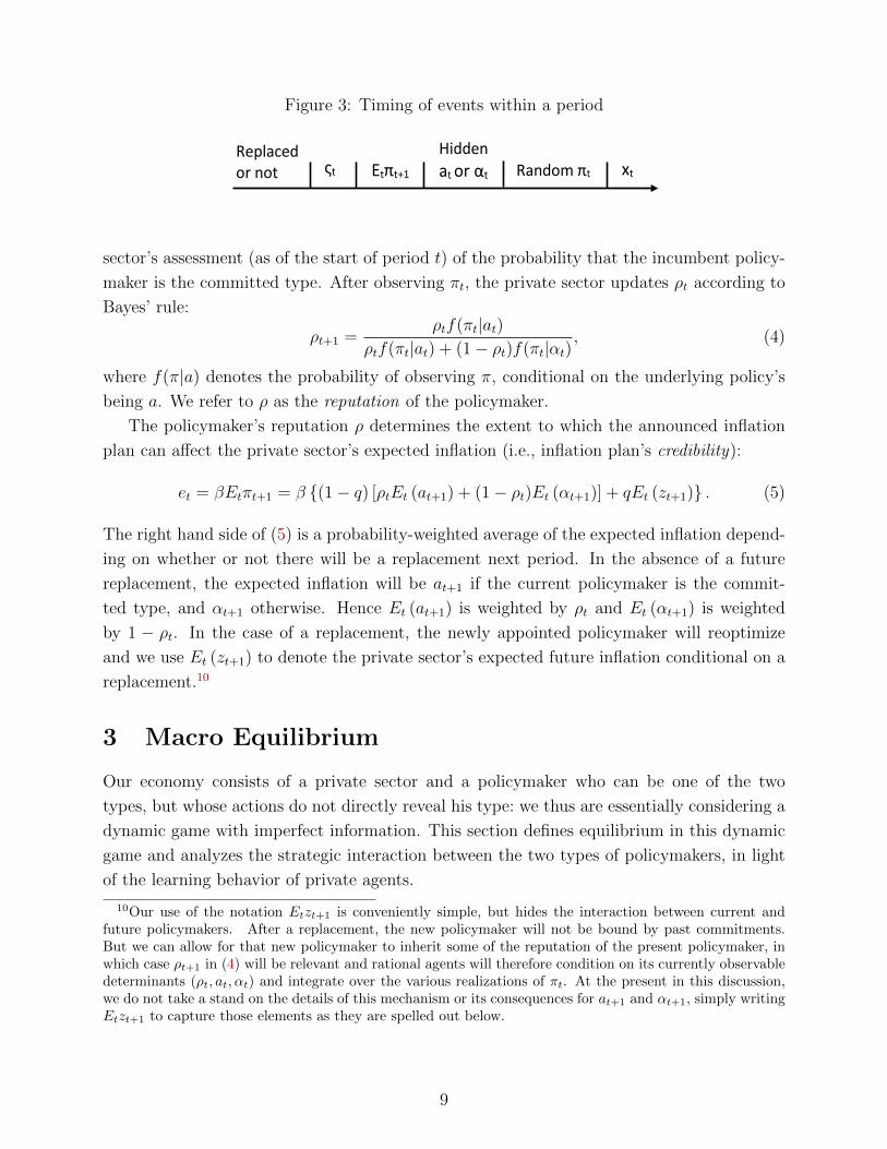
Figure 3: Timing of events within a period

Replaced or not ςt xt Random πt

Hidden at or αt Etπt+1

sector’s assessment (as of the start of period t) of the probability that the incumbent policy-

maker is the committed type. After observing πt, the private sector updates ρt according to

Bayes’ rule:

ρt+1 =ρtf(πt|at)

ρtf(πt|at) + (1− ρt)f(πt|αt), (4)

where f(π|a) denotes the probability of observing π, conditional on the underlying policy’s

being a. We refer to ρ as the reputation of the policymaker.

The policymaker’s reputation ρ determines the extent to which the announced inflation

plan can affect the private sector’s expected inflation (i.e., inflation plan’s credibility):

et = βEtπt+1 = β (1− q) [ρtEt (at+1) + (1− ρt)Et (αt+1)] + qEt (zt+1) . (5)

The right hand side of (5) is a probability-weighted average of the expected inflation depend-

ing on whether or not there will be a replacement next period. In the absence of a future

replacement, the expected inflation will be at+1 if the current policymaker is the commit-

ted type, and αt+1 otherwise. Hence Et (at+1) is weighted by ρt and Et (αt+1) is weighted

by 1 − ρt. In the case of a replacement, the newly appointed policymaker will reoptimize

and we use Et (zt+1) to denote the private sector’s expected future inflation conditional on a

replacement.10

3 Macro Equilibrium

Our economy consists of a private sector and a policymaker who can be one of the two

types, but whose actions do not directly reveal his type: we thus are essentially considering a

dynamic game with imperfect information. This section defines equilibrium in this dynamic

game and analyzes the strategic interaction between the two types of policymakers, in light

of the learning behavior of private agents.

10Our use of the notation Etzt+1 is conveniently simple, but hides the interaction between current andfuture policymakers. After a replacement, the new policymaker will not be bound by past commitments.But we can allow for that new policymaker to inherit some of the reputation of the present policymaker, inwhich case ρt+1 in (4) will be relevant and rational agents will therefore condition on its currently observabledeterminants (ρt, at, αt) and integrate over the various realizations of πt. At the present in this discussion,we do not take a stand on the details of this mechanism or its consequences for at+1 and αt+1, simply writingEtzt+1 to capture those elements as they are spelled out below.

9

3.1 Public Equilibria

Define the public history ht = ht−1, πt−1, ςt as the collection of all past realizations of

inflation rates and exogenous states. We restrict our attention to equilibria in which all

strategies are conditional only on the public history, i.e., “public strategies.”

Such a restriction is innocuous in our equilibrium analysis because: 1) the private sector’s

strategy has to be public since ht is the private sector’s information set; 2) the committed

type’s policy has to be public since it follows the announced policy plan, which needs to

be verifiable by the private sector; 3) given all the other player’s strategies are public, it is

also optimal for the opportunistic type to choose public strategies (Mailath and Samuelson

(2006)).

3.2 Perfect Bayesian

We further require the equilibrium of this imperfect information game to be perfect Bayesian.

That is, the beliefs of the private sector are consistent and the strategies of the two types of

policymakers satisfy sequential rationality.

3.2.1 Consistent beliefs

Expected inflation in (5) summarizes all the relevant beliefs of the private sector: (i) the

likelihood that the current policymaker is of the committed type; (ii) the expected inflation

if the current regime continues; and (iii) the expected inflation conditional on a replacement.

The private sector’s belief about the policymaker’s type follows Bayes’ rule as in (4). The

consistency restriction requires at and αt in (4) to be the equilibrium intended inflation of the

current committed and opportunistic policymaker, respectively. In turn, the private sector’s

belief ρ is also a function of the public history:

ρ (ht+1) = ρ (ht, πt) =ρ (ht) f(πt|a (ht))

ρ (ht) f(πt|a (ht)) + (1− ρ (ht))f(πt|α (ht)). (6)

The expected inflation if the current committed policymaker continues to be in charge will

follow the announced policy plan. The expected inflation if the current opportunistic pol-

icymaker continues to be in charge does not necessarily follow the announced policy plan,

neither does the expected inflation conditional on a future replacement. Hence, the private

sector needs to make conjectures on what they will be. In equilibrium, we impose ratio-

nal expectations in the sense that the conjectured inflations coincide with their equilibrium

counterparts.

Consequently, under the consistency restriction, the expected inflation et defined in (5) is

a function of ht with at+1, αt+1, and zt+1 in (5) replaced by their equilibrium counterparts,

and ρt following the updating rule (6):

e (ht) = β

ρ (ht)E [(1− q) a (ht+1) + qz (ht+1) |ht, τt = 1]

+(1− ρ (ht))E [(1− q)α (ht+1) + qz (ht+1) |ht, τt = 2]

. (7)

10

Notice that the expectation needs to be conditional on τt because the random inflation

outcome πt depends on the type-specific intended inflation. More specifically,

E [·|ht, τt = 1] =

∫(·) f (π|a (ht)) dπ and E [·|ht, τt = 2] =

∫(·) f (π|α (ht)) dπ.

3.2.2 Sequential rationality of the opportunistic type

The opportunistic policymaker takes expected inflation as given and chooses intended infla-

tion period-by-period to maximize his expected momentary utility

maxα

∫u (π, x, τ = 2) f (π|α) dπ,

subject to the NK Phillips curve (3). The quadratic objective leads to a linear decision rule:

αt = π∗ + ι+ Aβ[Etπt+1 − π∗] + Aςt (8)

where

A =ϑx

κ2 + ϑx< 1 and ι = A[κx∗2 − (1− β)π∗].

Top panel of Figure 4 illustrates the decision rule after setting cost-push shock ς = 0 and

using parameters of our benchmark calibration: π∗ = 1.5%, ι = .5%, A = .94 and β = .995.

If expected inflation is at the target, then the opportunistic type chooses α = π∗ + ι. So

we refer to ι as intrinsic inflation bias. The intersection of the decision rule (red solid line)

and the 45 degree line (black dash line) is the familiar full information Nash equilibrium:

αNE − π∗ =ι

1− Aβ, (9)

which we refer to as the Nash-Equilibrium (NE) inflation bias.

One key message is that NE inflation bias can be much greater than intrinsic inflation

bias when Aβ is close to 1. Another key message is implicit: the extent of inflation bias

α−π∗ depends on inflation expectations. If expectations are gradually adjusting to observed

inflation, then the optimal intended inflation of the opportunistic type also rise and fall

gradually with observed inflation, as illustrated in the bottom panel of Figure 4.11 Our

analysis below will incorporate a version of this mechanism in account for the rise and fall of

US inflation.

For the sake of future reference, we rewrite the decision rule (8) in terms of et := βEtπt+1:

α (e) = Ae+B (ς) (10)

where B (ς) = (1− Aβ)π∗ + ι+ Aς.

11Discussing a related model, Sargent and Soderstrom [2000] write: “The Nash outcome does dependcrucially on the assumption that the public’s expectations are fully rational. If instead it forms its expectationsadaptively, depending on the past inflation rate, one can imagine a dynamic version of the model. Thegovernment sets the inflation optimally given the public’s expectations. In the next period, the publicobserves the inflation rate and updates its expectations, and the government resets inflation at a new level,after which the public’s expectations are changed, etc. This leads to a process that eventually converges tothe Nash outcome, where the private sector’s expectations are realized, and the government sets the inflationrate optimally, given the expected rate of inflation.”

11

Figure 4: Optimal Response of Opportunistic Policy to Inflation Expectations

3.2.3 Sequential rationality of the committed type

The committed policymaker decides and announces all of his future state contingent policies

(a) at the beginning of his term and then subsequently executes these without fail. As a

result of his announcement, the committed state-contingent policy plan is public information

and has strategic power on private sector’s expectation and thus on the opportunistic type’s

intended inflations. In particular, the strategy of the committed type is sequentially rational

12

if it maximizes his expected payoff at the beginning of his term (dated as period 0),

E0∞∑t=0

βt1 (1− q)t∫u (πt, e (ht) , ςt, τt = 1) f (πt|at) dπt, (11)

where u (π, e, ς, τ = 1) is the momentary objective of the committed type with x replaced by

(π − e− ς) /κ. The committed type takes into account that (i) the private sector’s expec-

tation e (ht) is formed based on a consistent belief system (7), through which both his own

policies and the opportunistic policies affect how et responds to the past history ht, and (ii)

the opportunistic policy αt is sequentially rational, i.e., it satisfies (10), so that it optimally

respond to the expected inflation e (ht).

3.3 Public Perfect Bayesian Equilibrium

We can now define the Public Perfect Bayesian Equilibrium for this dynamic game.

Definition 1. A Public Perfect Bayesian Equilibrium is a set of functions e(ht), ρ(ht),α(ht), a(ht) and z(ht) such that:

i) given the policymaker’s strategies, α(ht), a(ht), and z(ht), and the private sector’sbelief function ρ(ht), the private sector’s expected inflation function e(ht) satisfies (7); andits belief function ρ(ht+1) is updated according to (6); and

ii) given the expected inflation function, e(ht), the strategy for the opportunistic typepolicymaker, α(ht) satisfies (10); and

iii) the strategy for the committed type policymaker, a(ht), maximizes his expected payoff(11); and

iv) the expected inflation conditional on a replacement, z(ht), is consistent with a(ht),α(ht) and ρ(ht).

4 Recursive optimal policy design

The Public Perfect Bayesian equilibrium in this game can be constructed by a two-stage

approach. In the first stage, a within-regime equilibrium e(ht), ρ(ht), α(ht), a(ht) is con-

structed taking as given the expected inflation z(ht) conditional on a replacement of pol-

icymaker (i.e., a regime change). The second stage is a cross-regime fixed point problem.

Recall that the Public Perfect Bayesian equilibrium requires the expected inflation z(ht) to

be consistent with the equilibrium a(ht), α(ht) and ρ(ht) obtained in the first stage. The

second stage thus is to find a fixed point between z(ht) and a(ht), α(ht), ρ(ht).Constructing the first-stage within-regime equilibrium can be usefully viewed as solving

a principal-agent problem. The policymaker of the committed type is the principal. He

maximizes the objective (11) by choosing the future actions of his own and the future actions

for the two agents – the private sector and the policymaker of the opportunistic type. In

choosing the future actions of the two agents, the principal has to respect two sets of incen-

tive compatibility constraints. The incentive compatibility constraints for the private sector

13

comprises of both the consistent belief constraint (6) and the rational expectation constraint

(7). The incentive compatibility constraint for the opportunistic type is his optimal response

to the expected inflation (10).

In the following proposition, we formulate the optimal policy problem of the principal

– the committed policymaker – in a recursive form. Among three incentive compatibility

constraints, the rational expectation constraint (7) on the private sector is forward-looking

and needs to be transformed to yield a recursive specification. Following the approach laid

out by Kydland and Prescott (1980), Marcet and Marimon (2019) and others,12 we cast the

Lagrangian components associated with the forward-looking constraint (7) in recursive form

by (i) application of the law of iterated expectations; and (ii) appropriate rearrangement of

expected discounted sums. What is unusual about the current model is that the committed

policymaker and the private sector not only have different time discount factors, but they

also disagree on the probability distribution of inflation outcome π: the density of π is

f (π|a) according to the committed policymaker, but ρf (π|a) + (1− ρ) f (π|α) according to

the private sector.

Proposition 1. Given z∗(ς, ρ), the within-regime equilibrium can be obtained as the solu-tion to the following recursive optimization:

W (ς, ρ, µ) = minγ

maxa,α,eu (a, e, ς, τ = 1) + (γe+ µω) +

β1 (1− q)∫ ∑

ς′

ϕ (ς ′; ς)W (ς ′, ρ′, µ′) f (π|a) dπ, (12)

where

ω = −

(1− q) a+ qz∗(ς, ρ) +1− ρρ

[(1− q)α + qz∗(ς, ρ)]

(13)

subject to

α = Ae+B (ς) (14)

µ′ =β

β1 (1− q)γρ, with µ0 = 0 (15)

ρ′ =ρf(π|a)

ρf(π|a) + (1− ρ) f(π|α)(16)

In this recursive program, there are familiar components given prior research using this

approach, and some unfamiliar ones due to unique features of our model.

The first component u (a, e, ς, τ = 1) is the committed policymaker’s expected momentary

objective:∫u (π, e, ς, τ = 1) f (π|a) dπ.

The second component (γe+ µω) arise from the forward-looking rational expectation

constraint (7).13 γ is the Lagrangian multiplier attached to the constraint and the pseudo

12See also Chang (1998) and Phelan and Stacchetti (2001).13The specific form of this problem reflects our efforts to minimize state variables, as explained in detail

in Appendix B.

14

state variable µ serves to record the effect of past promises made by the committed type in

his management of expectations. Hence, the next-period pseudo state µ′ evolves according

(15) that keeps track of the shadow value of current promise γ, the effect of current promise

on expected inflation measured by ρ, and weight adjustment to reflect different time discount

factors between the committed policymaker and the private sector. We assume that a new

policymaker is not held accountable for his predecessor’s promises, so the initial value of the

pseudo-state µ is set to be zero.

It is worth mentioning that, in our setting with two types of policymakers and stochastic

replacement, the term ω defined in (13) contains not only the promise by the committed

policymaker, but also two other inflation rates: the intended inflation α of the opportunistic

policymaker, and the expected inflation z conditional on a replacement. The weights attached

to a, α, and z reflect the exogenous replacement probability q, the endogenous reputational

state ρ, and different probability beliefs about inflation outcome π held by the committed

policymaker and the private sector.

The reputation state ρ evolves according to Bayes’ rule (16), which depends on the random

inflation outcome π, promised inflation a by the committed type, and rationally expected

intended inflation α by the opportunistic type. The reputation state enters the committed

policymaker’s payoff by determining how much expected inflation e can be affected by his

promise, relative to by the opportunistic type’s intended inflation, i.e., the RHS of (13). This

effect of reputation and its implications for the optimal committed policy are studied in our

prior work Lu et al. (2016).

Compared to Lu et al. (2016) in which α is assumed to follow a mechanical rule, the novel

component of this study is that α is chosen optimally by the opportunistic type in response to

the private sector’s expected inflation, summarized in (14). This optimal response creates two

additional channels through which managing expectations matters for the committed type’s

payoff: (i) the expectation anchoring channel by affecting α in ω; and (ii) the reputation

building channel by affecting α in the state evolution equation of ρ (16).

The second stage solves a cross-regime fixed point problem, similar to Schaumburg and

Tambalotti (2007). It requires the expected inflation z∗(ς, ρ) conditional on a replacement

to satisfy the following fixed point

z∗(ς, ρ) = ρ0a∗ (ς, ρ0, 0; z∗(ς, ρ)) + (1− ρ0)α∗ (ς, ρ0, 0; z∗(ς, ρ)) (17)

where a∗(.) and α∗(.) are the within-period equilibrium obtained in the recursive program

(12) given z∗(ς, ρ). ρ0 is the new policymaker’s initial reputation and a function of ρ as we

allow the new policymaker to inherit his reputation partially from his predecessor. Moreover,

the initial value of the pseudo-state µ in the new regime is set to zero.

15

4.1 Tradeoffs in managing expectations

Using this framework, we can discuss the tradeoffs that the committed policymaker faces

in managing expectations of the private sector. We start with some familiar elements from

textbook analyses such as those of Woodford (2003), Walsh (2010), and Gali (2015), then

move to the elements related to more recent literature such as Schaumburg and Tambalotti

(2007) and Lu et al. (2016). We end with the elements that are unique to this paper – the

incentive compatibility of the opportunistic type’s action.

Stimulating real activity In a full commitment benchmark, optimal monetary policy

with no exogenous inflation shocks (ς = 0), no regime changes (q = 0) and perfect credibility

(ρ = 1) is well understood to be history dependent, i.e., there is a path of initially high but

declining inflation that we call “startup inflation”. In each period of the inflation path, the

expected inflation is engineered to be lower than the current inflation e < π, so that there is

a stimulation of real activity brought about by the optimal policy.

In the current recursive framework, this history dependence is captured by the dependence

of the policy a on the pseudo state variable µ that transits endogenously from an initial

condition µ0 = 0. The term −µa in (13) captures the effect of past commitments: a greater

value of µ makes it less desirable to raise current inflation from 0. As we will see later, in

the full commitment benchmark, the pseudo state variable µ rises along the transition path

towards its positive steady state value, and the policy action a declines, ultimately converging

to the long-term inflation target π∗.

Smoothing out shocks With exogenous cost-push shocks (ς 6= 0) in the Phillips curve (3),

expectation management can smooth out the effect of these shocks on output. For example,

after a positive cost-push shock (ς > 0), output will be reduced if a and e are held fixed. It

is therefore desirable to partly accommodate the shock (raising a) and, to also stimulate real

activity by reducing expected inflation e. Technically, a positive cost-push shock produces

a contemporaneous increase in the Lagrangian multiplier γ, which translates into a higher

pseudo-state variable µ′ in the following period and a decrease in the optimal policy a′, thus

ratifying the downward movement in expected inflation e.

Accommodating imperfect credibility With prospective regime change (q > 0), as

stressed by the “loose commitment” approach:14 the future is discounted more heavily in the

objective (12) and the optimal policies of a successor z appear in forward-looking expectations

(13). With unobservable policymaker type (ρ < 1), as stressed by the reputation literature

on monetary policy:15 the intended inflation of an opportunistic policymaker α enters the

14The “loose commitment” approach is originally developed by Roberds (1987) and more recently extendedby Schaumburg and Tambalotti (2007) and Debortoli et al. (2012).

15Optimal committed monetary policy under imperfect credibility is studied by Cukierman and Liviatan(1991) and King et al. (2008) in settings with the Lucas-Barro-Gordon Phillips curve, and by Lu et al. (2016)

16

expectations (13). In both cases, the committed policymaker in the current regime needs

to reckon that part of the private sector’s expected inflation cannot be managed by his

own promised future policies, but rather by future policies of a policymaker that prefers

higher inflation. As a result, the committed policymaker needs a greater change of promised

future policy to achieve the same effect on the expectations, and a higher current policy to

accommodate the negative impact of a higher expected inflation on output.

Building reputation In settings where the private sector is learning about the policy-

maker’s type, there is an additional state variable ρ relative to the standard NK framework.

The level of ρ enters two parts of the recursive program. First, it determines the relative

weight on the opportunistic type’s intended inflation α in the forward-looking expectation

constraint (13) – a higher ρ reduces the impact of α on the committed policymaker’s payoff.

Second, ρ enters the evolution of the pseudo-state variable µ′ (15) – a higher ρ implies a

higher pseudo-state variable µ′ in the following period and in turn a decrease in the optimal

policy a′. Intuitively, a higher ρ enables the committed policymaker to manage the private

sector’s expected inflation more effectively with his own future committed policies. Increasing

ρ (building reputation) is therefore a desirable objective for the committed type.

Through the Bayesian learning rule (16), the evolution of ρ is affected by both the com-

mitted policy a and the opportunistic type’s intended inflation α. In a setting where α

mechanically follows a policy rule α(ς), Lu et al. (2016) shows that there is a tradeoff be-

tween building reputation (accelerating learning) and accommodating imperfect credibility in

the optimal committed policy design, and over a large empirically relevant parameter space,

the reputation building effect dominates.

Incentive compatible opportunistic intended inflation In the current model, the op-

portunistic type’s intended inflation optimally responds to the contemporaneous expected

inflation. At the same time, the private sector’s expected inflation is affected by the op-

portunistic type’s future intended inflation. This dynamic inter-dependence between the

opportunistic intended inflation and the private sector’s expected inflation provides the com-

mitted policymaker with an additional channel of managing expectations. More specifically,

by designing his own path of committed policies, the committed policymaker can affect the

expected inflation, which in turn determines the intended inflation of the opportunistic type,

which can be made closer to or further away from the committed policy. If the opportunistic

intended inflation is made closer to the committed policy, it will mitigate the adverse impact

of imperfect credibility on expected inflation. Too see that, suppose that the opportunis-

tic intended inflation is exactly equal to the committed policy, then expected inflation will

be perfectly aligned with the promised committed policy, as if the committed policymaker

has the full credibility. If the opportunistic intended inflation is made further away from

in a setting with the forward-looking New Keynesian Phillips curve.

17

the committed policy, it will make the realized inflation outcome π more informative about

the policymaker’s type and thus accelerate private sector’s learning. Faster learning makes

expectations more manageable for the committed policymaker in the future. Thus, such an

indirect influence on the opportunistic intended inflation gives the committed policymaker

more strategic power in balancing the tradeoff between building reputation (accelerating

learning) and accommodating imperfect credibility.

4.2 Policy Design with Incentive Compatibility

The committed policymaker’s choice of expected inflation e is a key part of the recursive

optimization. In choosing e, the committed policymaker has to respect the forward-looking

rational expectation constraint (7), where the expected future inflations (a, α, z) are to follow

their equilibrium strategies. The following lemma shows how this forward-looking rational

expectation constraint (7) helps to reduce the determinants of e to only 4 variables.

Lemma 1. Given the state variables (ς, ρ), and the equilibrium strategies a∗ (ς, ρ, µ),α∗ (ς, ρ, µ) and z∗ (ς, ρ), the rationally expected inflation is uniquely determined by the con-temporaneous difference between the intended inflations of the two types δ = a−α, and thenext-period pseudo-state variable µ′.

e = e (δ, µ′; ς, ρ) = βρ

∫M1(ς, b (σε, σε+ δ, ρ) , µ′)φ (ε) dε+ (18)

β(1− ρ)

∫M2(ς, b (σε− δ, σε, ρ) , µ′)φ (ε) dε; (19)

where φ (·) denotes the standard normal density function;

M1 (ς, ρ′, µ′) : =∑ς′

ϕ (ς ′; ς) [(1− q) a∗ (ς ′, ρ′, µ′) + qz∗ (ς ′, ρ′)] ;

M2 (ς, ρ′, µ′) : =∑ς′

ϕ (ς ′; ς) [(1− q)α∗ (ς ′, ρ′, µ′) + qz∗ (ς ′, ρ′)] ;

b (σε, σε+ δ, ρ) =ρ

ρ+ (1− ρ)φ(σε+δσ

)/φ(σεσ

) is ρ′ conditional on τ = 1;

b (σε− δ, σε, ρ) =ρ

ρ+ (1− ρ)φ(σεσ

)/φ(σε−δσ

) is ρ′ conditional on τ = 2.

Lemma 1 says there are two channels through which the committed policymaker can in-

fluence private sector’s expected inflation. The first channel is through the contemporaneous

difference between his own committed policy and the intended inflation of the opportunistic

type. This is the learning channel as a larger difference in intended inflations of the two

types makes the private sector learns faster about the current policymaker’s type. The sec-

ond channel is through the next-period pseudo-state variable µ′ that captures the shadow

value of the pre-commitment. This is the expectation anchoring channel. A higher µ′ implies

lower next-period intended policies of both types. Notice that due to the forward-looking

18

nature of the expected inflation, it is the next-period µ rather than the current-period µ that

determines the expected inflation.

Lemma 1 also implies that when the committed policymaker chooses the expected inflation

e, he simultaneously determines the opportunistic intended inflation α via the opportunistic

type’s optimal response to the inflation expectation, (14), and the committed policy a via δ

– the contemporaneous difference in intended inflations: a = α + δ. This observation allows

us to rewrite the momentary utility function u and the term ω in the recursive program (12)

by replacing a with α + δ, α with Ae + B(ς), and e with e(δ, µ′; ς, ρ) as in Lemma 1. As a

result, the recursive program is simplified from choosing (γ, a, α, e) to merely choosing e or

equivalently (δ, µ′). The following proposition states the simplified recursive program:

Proposition 2. Given z∗(ς, ρ) and U (ς, ρ, µ), the recursive optimization (12) reduces to

W (ς, ρ, µ) = maxδ,µ′

u (δ, µ′) + µω (δ, µ′) + β1 (1− q) Ω (δ, µ′) (20)

where

u (δ, µ′) : = u (Ae+B(ς) + δ, e, ς, τ = 1) (21)

ω (δ, µ′) : = −1

ρ[(1− q) (Ae+B(ς)) + qz∗ (ς, ρ)]− (1− q) δ (22)

Ω (δ, µ′) =

∫ ∑ς′

ϕ (ς ′; ς)U (ς ′, b (σε, σε+ δ, ρ) , µ′)φ(ε)dε (23)

with e = e(δ, µ′; ς, ρ).

The continuation value function U (ς, ρ, µ) satisfies the following fixed point problem

U (ς, ρ, µ) = W (ς, ρ, µ)− µω(δ∗, µ′∗) (24)

where W (ς, ρ, µ), δ∗ and µ′∗ are the solution to the simplified recursive program (20) com-

puted conditional on U (ς, ρ, µ).

4.3 Summary and numerical algorithm

Using the rational expectation constraint (7), we have shown that given the state vari-

ables (ς, ρ) and the future policies following their equilibrium strategies, the private sec-

tor’s expected inflation e is a function of δ = a − α, the contemporaneous difference be-

tween the committed and the opportunistic types’ intended policies, and µ′, the next-

period pseudo-state variable. Such a rational expectation function e (δ, µ′; ς, ρ) implies an

incentive compatible opportunistic policy function α (δ, µ′; ς, ρ) via the opportunistic type’s

optimal response to the inflation expectation, (14), and a committed policy function via

a (δ, µ′; ς, ρ) = α (δ, µ′; ς, ρ) + δ.

We have also shown that after substituting out e in the recursive optimization (12) with

the rational expectation function e (δ, µ′; ς, ρ), the recursive optimization can be simplified to

19

(20), where the optimal pair (δ, µ′) determines all equilibrium strategies in our Public Perfect

Bayesian Equilibrium.

The numerical algorithm for computing our Public Perfect Bayesian Equilibrium follows

similar steps. With a set of guessed functions z (ς, ρ), a(ς, ρ, µ), α(ς, ρ, µ) and U(ρ, η, ς),

1) we obtain the rational expectation function e(δ, µ′; ς, ρ) and the expected continuation

function Ω (δ, µ′; ς, ρ) via (18) and (23);

2) we use (14) to determine α (δ, µ′; ς, ρ) and a (δ, µ′; ς, ρ) = α (δ, µ′; ς, ρ) + δ;

3) we evaluate the committed type’s payoff as in (20) conditional on each pair (δ, µ′);

4) we identify (δ, µ′) that maximizes the committed type’s payoff conditional on (ς, ρ, µ);

5) we use the optimal (δ, µ′) to update the guessed functions.

Iterate until the policy functions converge.

5 Equilibrium Policies

In this section, we use a calibrated version of the model to shed light on aspects of the U.S.

inflation experience in the 70s and 80s. We start by explaining our calibration strategy. We

then show that the equilibrium dynamics in an opportunistic regime with high initial reputa-

tion, and in a committed regime with low initial reputation, and how they can qualitatively

resembles the U.S. inflation experience during the “Great Inflation” in 70s, and during the

“Volcker Disinflation” in 80s, respectively.

5.1 Calibration

Table 1: Benchmark calibration

β, β1 Discount factor 0.995q Replacement probability 0.03ρ0 Initial reputation after replacement 1% + 0.9ρ−1ϑx Output weight 0.1κ PC output slope 0.08x∗1 Committed type’s output target 1.7%x∗2 Opportunistic type’s output target 1.75%π∗ Inflation target 1.5%δ Persistence of cost-push shock 0.7σξ Std of cost-push innovation 0.7%σε Std of implementation error 1.2%

One period is one quarter in our calibration and the parameter values are summarized in

Table 1. The committed policymaker and the private sector share the same time discount

factor, which implies a steady-state interest rate of about 2% annually. The replacement

probability q is set to 0.03 so that the average tenure of a policymaker in our model is 8

20

years. The newly appointed policymaker has an initial reputation equal to 1% + 0.9ρ−1, so

that the plausible range of initial reputation is [1%, 91%].

Our calibration strategy is to match the Great Inflation experience in the U.S. in 70s and

the Volcker disinflation in 80s. To this end, we obtain the slope of the Phillips Curve κ from

the empirical relation between unemployment and inflation in the 1950s and 1960s, when a

1% increase in unemployment led to about 0.54% - 0.65% increase in inflation, depending

on whether inflation is measured year over year (standard Fed practice) or quarterly at an

annual rate. Using Okun’s law, a 1% increase in the unemployment rate is associated with a

2% increase in the output gap (i.e. Okun’s coefficient is 2). This suggests that the empirical

relevant range of κ in our Phillips curve is between 0.068 and 0.081.16

Turning to relative weight of output in policymaker’s objective function with quarterly

inflation variability, ϑx = 0.1 is equivalent to a weight equal to 1.6 in an objective with annual

inflation variability. Based on Okun’s law, the variance of the output gap is about 4 times

that of the unemployment gap. Therefore, our choice of ϑx = 0.1 means that the weight on

stabilizing unemployment is 6.4 times the weight on stabilizing annual inflation. To put such

a number into perspective, the weight on stabilizing unemployment v.s. stabilizing inflation

in the literature varies from 1(Brayton et al. (2014)) to 16 (Orphanides and Williams (2013)).

To match the peak of the Great Inflation, we set a NE inflation bias (9) equal to 8%.

The slope of Phillips curve κ and the output weight ϑx implies that the response coefficient

of opportunistic policy A in (10) is 0.94, which in turns determines the intrinsic inflation

bias ι = 0.52%. The intrinsic inflation bias allows us to back out the opportunistic type’s

output target, assuming the inflation target is 1.5% (annualized quarterly rate). We then set

a slightly lower but essentially the same output target of the committed type.17

Many studies of inflation dynamics incorporated “price shocks” during the Great Inflation,

establish a now standard practice. A prominent one, used by Gordon and King (1982) and

Watson (2014), is a ”Food and Energy price shock” constructed as the difference between

the growth rate of the overall personal consumption deflator and its counterpart excluding

food and energy. We then take a 2-quarter moving average to smooth the series and scale it

by 2/3 since personal consumption expenditure is about two-thirds of GDP. This would be

one measure of the shock ς.18 The persistence and standard deviation of ς in our calibration

matches their empirical counterparts of this series.

Another important parameter is the standard deviation of the implementation error σε.

We obtain it assuming the inflation policies in 1970s were implemented by an opportunistic

policymaker who was optimally responding to the expected inflation measured by the SPF

and the cost-push shock measured by the food-energy inflation rates. The difference between

such an opportunistic inflation policy and the actual inflation (measure by quarterly change

in GDP deflator) is interpreted as the implementation errors. We then identify the time

16These empirical relations can be found in Figures 15 and 16 in the Appendix.17Due to a computational technicality, x∗1 needs to be different from x∗2.18The series is plotted in Figure 17 in the Appendix.

21

window when the mean of implementation errors equals zero, and use that time window to

compute the standard deviation of the implementation errors, which turns out to be around

1.2% (annualized quarterly rate).19

5.2 Equilibrium dynamics with opportunistic type in charge

We start by describing the equilibrium dynamics of a new regime when an opportunistic

policymaker inherits good, but not perfect reputation. Our first focus is on the transitional

dynamics that arise when all shocks are set to zero in all periods. We then show how the

economy responds when there is a 1% cost push shock during the middle of this transition. We

find three phases that qualitatively resemble the U.S. inflation during the “Great Inflation” .

In interpreting dynamic outcomes here and below, it is important to remember that there

are no structural sources of inflation persistence in this New Keynesian model under com-

mitment.20 Yet, one should also bear in mind the NK optimal policy framework exhibits

“startup inflation”: with replacement but without learning, a new committed policymaker

will choose to set inflation initially above its long-run optimal level π∗ because there are

short-run benefits from stimulating the real economy through a path of high, but declin-

ing inflation.21 As we will see, more elaborate dynamics arise with endogenously evolving

reputation when there is an opportunistic policymaker in charge.

5.2.1 Transitional dynamics

Figure 5 plots the transitional dynamics of various inflation rates, the output gap x, and

reputation ρ: : it also establishes some conventions that we will follow in subsequent figures.

In the left component of the panel, the red solid line is the equilibrium opportunistic policy

α when there are no shocks – the realized inflation rate – and we will always use red for α.

Expected inflation e will always be a solid blue line in the model and when we capture it with

SPF forecasts. We will use green for the committed policy a throughout, but we represent

a as a dashed line in this Figure because it is not an observable variable. Instead, it is the

committed policy a as rationally perceived by the private sector, i.e., it is what a committed

type would do in when confronted with this inflation history.

To serve as benchmarks, we also plot the opportunistic policy α under the polar assump-

tions that ρ = 0 and ρ = 1. If ρ = 0, i.e., agents know that there is an opportunistic poli-

cymaker in place: note that this α solution, represented with a dash-dot black line, features

the NE bias discussed earlier. Another useful benchmark is the behavior of the opportunistic

19The moving average and standard deviation are plotted in Figure 18 in the Appendix.20By contrast, hybrid versions of the NKPC take the form

πt = γfEtπt+1 + γbπt−1 + ςt

with structural inflation persistence implying γb > 0 and conventional micro-based specifications implyingthat γf + γb is close to, but less than one. (see addref)

21See, for example, Schaumburg and Tambalotti (2007).

22

Figure 5: Transitional Dynamics in Opportunistic Regime with ρ0 = 0.8

Figure 6: Dynamic response to cost push shock in Opportunistic Regime with ρ0 = 0.8

type if expected inflation follows the path chosen by the committed type without reputation

concerns: we plot this using a dashed black line and label it as ρ = 1. Such a policy outcome

can never occur, of course, but it is a useful reference point for high ρ. Finally, the dotted

black line is the constant inflation target π∗.

The equilibrium opportunistic policy α (red) starts at a rate around 3.5% and decreases

gradually toward the inflation target for several years, as a consequence of two basic and

important properties of our framework. First, as discussed earlier, with full commitment, a

new committed policymaker chooses an inflation plan that features start-up inflation. Under

this plan, expected inflation is also high and declining, a feature that is partially inherited

23

by rational expectations when there is a high likelihood of a committed policymaker being

in place (a good initial reputation). Second, confronted with such relatively low inflation

expectations, our opportunistic policymaker also chooses a low inflation given the response

function α−π∗ = A(e−βπ∗)+ι because intrinsic inflation bias is small (recall Figure 4). The

roughly 3.5% initial level includes the 1.5% inflation target, 0.5% intrinsic inflation bias and

1.5% response to expected inflation, which is essentially at the level under full commitment

(the red and black dashed lines are therefore close to each other in early periods).

During an initial phase, which is quite lengthy in Figure 5, there continues to be little

difference between α and a, so that there is little reputation evolution in the bottom right-

hand panel. Real output is high because α > e and there is a relatively flat Phillips curve

(x = 1κ(π− e)). Early on, the equilibrium opportunistic policy α (red) tracks the dashed line

because expectations are close to those arising under policy with full commitment.

But, over time, a wider gap between a and observed inflation (π = α) arises because a

committed type would reduce inflation toward π∗. As the gap widens, reputation declines,

expectations rise, and the opportunistic policymaker increases α in response given α− π∗ =

A(e−βπ∗)+ι. There is a positive feedback mechanism – highlighted in Figure 4 – that drives

inflation and expectations toward their Nash Equilibrium levels. Output declines as actual

and expected inflation become more closely aligned.22 This “stagflation” is the terminal

phase of our model’s inflationary process.

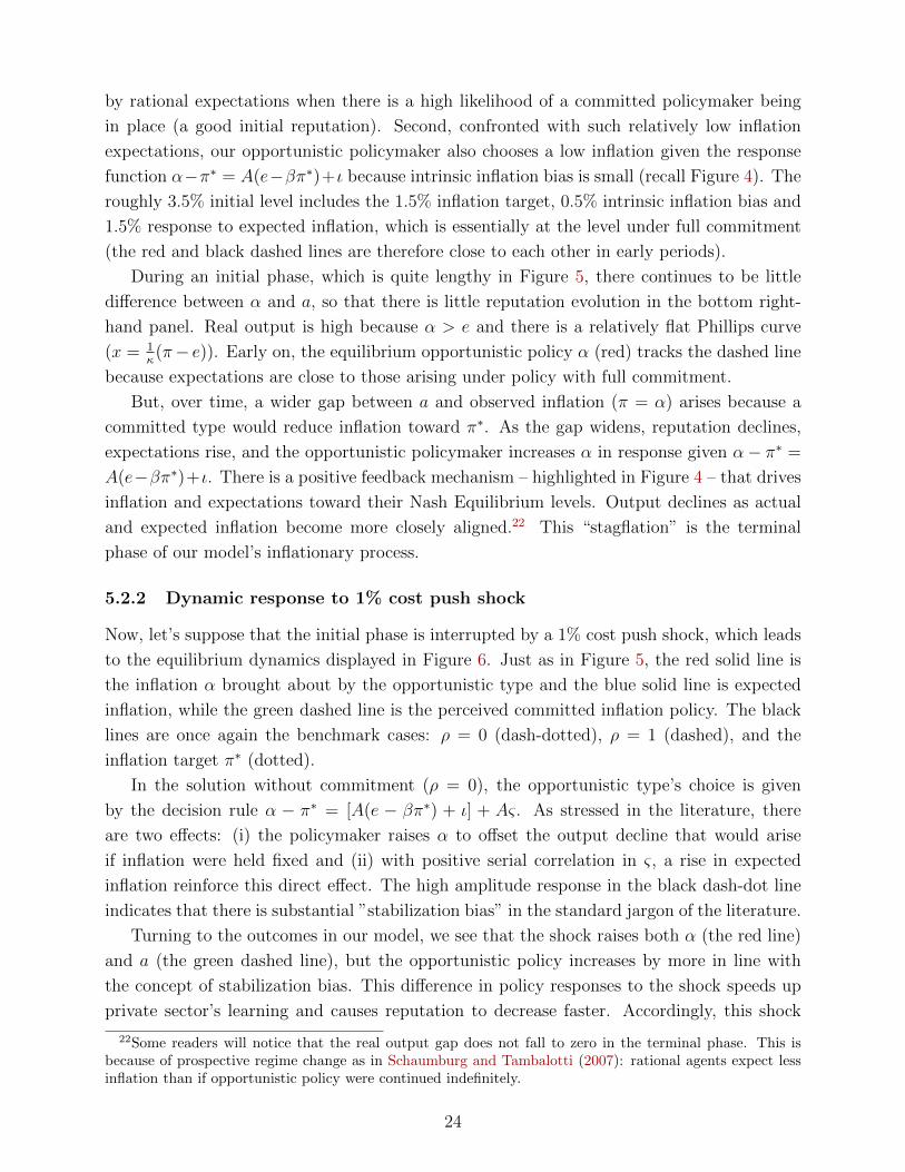
5.2.2 Dynamic response to 1% cost push shock

Now, let’s suppose that the initial phase is interrupted by a 1% cost push shock, which leads

to the equilibrium dynamics displayed in Figure 6. Just as in Figure 5, the red solid line is

the inflation α brought about by the opportunistic type and the blue solid line is expected

inflation, while the green dashed line is the perceived committed inflation policy. The black

lines are once again the benchmark cases: ρ = 0 (dash-dotted), ρ = 1 (dashed), and the

inflation target π∗ (dotted).

In the solution without commitment (ρ = 0), the opportunistic type’s choice is given

by the decision rule α − π∗ = [A(e − βπ∗) + ι] + Aς. As stressed in the literature, there

are two effects: (i) the policymaker raises α to offset the output decline that would arise

if inflation were held fixed and (ii) with positive serial correlation in ς, a rise in expected

inflation reinforce this direct effect. The high amplitude response in the black dash-dot line

indicates that there is substantial ”stabilization bias” in the standard jargon of the literature.

Turning to the outcomes in our model, we see that the shock raises both α (the red line)

and a (the green dashed line), but the opportunistic policy increases by more in line with

the concept of stabilization bias. This difference in policy responses to the shock speeds up

private sector’s learning and causes reputation to decrease faster. Accordingly, this shock

22Some readers will notice that the real output gap does not fall to zero in the terminal phase. This isbecause of prospective regime change as in Schaumburg and Tambalotti (2007): rational agents expect lessinflation than if opportunistic policy were continued indefinitely.

24

Figure 7: Great Inflation: inflation, expected inflation and food-energy price

leads to a rise in expected inflation (the blue line) which exhibits a higher persistence than

the shock itself does. Afterward, expected inflation and opportunistic policy are on a higher

plateau for the duration of the initial phase, given an erosion of reputation. Note also that

the terminal phase has been brought forward in time.

5.2.3 The Great Inflation

In Figure 7, we plot the time series of inflation, expected inflation, and food-energy price

during the “Great Inflation” in the 1970s. At least three features of the “Great Inflation”

experience are qualitatively replicated by the equilibrium dynamics with high initial reputa-

tion in Figure 6. First, the realized and expected inflation remained relatively low and stable

until 1972 when the food and energy price shock picked up. Second, the food and energy

price shock increased both actual and expected inflation with the former above the latter

between 1972 and 1975. Third, the temporary food and energy price shock has caused a

permanent increase in the expected inflation from below 4% before 1972 to around 6% after

1975. Moreover, after the food and energy price shock, the expected inflation has caught up

with the realized inflation.

5.3 Equilibrium dynamics with committed type in charge

We now present equilibrium dynamics of a new regime with a committed policymaker and a

low initial reputation. We start with the transitional dynamics where all the realized shocks

are set to zero, and then proceed to the dynamic response to a series of negative 1% cost

push shocks. We end with showing the time series of realized inflation, expected inflation,

and food-energy price shocks during the “Volcker Disinflation” in the 1980s.

25

Figure 8: Transitional Dynamic in Committed Regime with ρ0 = 0.2

Figure 9: Dynamic response to cost push shocks in Committed Regime with ρ0 = 0.2

5.3.1 Transitional dynamics

Figure 8 plots the transitional dynamics of various inflation rates, output gap x, and repu-

tation ρ under a new committed regime. In the left panel, the green solid line is the realized

inflation rate (i.e., the equilibrium committed policy a); the blue solid line is the expected

inflation e; and the red dashed line is the perceived opportunistic policy α.

The cases with ρ = 0 (black dash-dotted line) and ρ = 1 (black dashed line) are refer-

ence points corresponding to standard solution under full discretion and full commitment,

respectively. The solution under full discretion is the same as the one in Figure 5 where the

26

policymaker is the opportunistic type. In this sense, the committed policymaker without

any reputation behaves identically to the opportunistic policymaker. The full commitment

solution features an initial interval of high but declining inflation (”start-up inflation”) with

the rate gradually converging to the target 1.5% (black dotted line). Such a gradual disin-

flation is driven by the incentive to temporarily sustain output gap above zero because the

committed type regards a zero output gap being inefficiently low (i.e., x∗1 > 0). The output

gap in steady state falls below zero as the private agents expect a possible future regime

switch and the expected inflation of the new regime will be higher than the inflation target.

Turning to the case with ρ0 = 0.2, the most striking feature, relative to Figure 5, is that

all inflation rates start at levels that are above 5%. Hence the optimal inflation policy by a

committed policymaker could be higher than the optimal inflation policy by an opportunistic

policymaker, if the former is endowed with a much lower reputation. Secondly, the optimal

committed policy path lies above the full commitment solution, meaning that with low initial

reputation, it is not optimal for the committed policymaker to reduce inflation too fast.

Third, the initial gap between the committed policy and perceived opportunistic policy is

much larger than in Figure 5, which induces faster learning at a cost of significant output

loss. This is in contrast to the costless disinflation in the case of ρ = 1. With low initial

reputation, the committed policymaker faces inflation expectations that are very sticky (in

terms of not being responsive to his future policy announcement) and are anchored by the

perceived opportunistic policy. If the committed policymaker signals his type by lowering the

committed policy relative to the opportunistic policy, the realized policy will be lower than

the inflation expectations, and hence an output loss occurs. Fourth, the policy gap between

the committed policy and the perceived opportunistic policy shrinks over time, resulting in a

slowdown of learning after the initial boost of reputation. Consequently, it takes more than

4 years for the private sector to learn that they are facing a committed policymaker.

5.3.2 Dynamic response to -1% cost push shock

Figure 9 show the dynamic response to consecutive periods of -1% cost-push shocks from

t = 1 to t = 5. Same as in Figure 8, the green and the blue solid lines are the realized and

expected inflation, respectively; the red dashed line is the perceived opportunistic inflation

policy. The black lines are benchmarks for the optimal committed policy a in the polar

reputation cases: ρ = 0 (dash-dotted) and ρ = 1 (dashed). The inflation target π∗ is plotted

using the black dotted line.

In response to the series of negative cost-push shocks, all the inflation rates shift down-

wards to varying degrees. The optimal committed policy a in case of ρ = 0, similar to the

opportunistic regime response shown in Figure 6, simply reflects the persistence of the shock

with the contemporaneous impact of the shock split to both inflation and output. The case

of ρ = 1 has a mitigated response in both inflation and output, thanks to the ability of the

policymaker to manage expectations as an additional channel of shock smoothing.

27

Figure 10: Volcker Disinflation: inflation, expected inflation and food-energy price

Turning to the outcomes in our model, both the committed policy a and the opportunistic

policy α fall below expected inflation e in response to the series of negative price shocks. This

is because the private agents keep expecting a mean-reverting of the shock but are constantly

surprised by the constant negative shocks during the period. Moreover, the committed policy

a falls less than the opportunistic policy α, for the same reason as why the optimal a when

ρ = 1 responds less to the shock than when ρ = 0. That is, the committed policymaker

can manage expectations as an additional channel to smooth shock but the opportunistic

policymaker cannot. As a result, the policy gap between the two types of policymaker

shrinks and it slows down the private sector’s learning. Comparing the reputation evolution

to its counterpart in Figure 9, the series of negative cost-push shocks makes the reputation

grow at a slower rate.

5.3.3 The Volcker Disinflation

Figure 10 plots the U.S. inflation experience during the period when Paul Volcker served

as Chair of the Federal Reserve. Starting from 1981, both inflation and expected inflation

declined with the realized inflation lower than the expected inflation. Moreover, this disin-

flation episode was associated with a recession that last more than a year. Furthermore, the

food-energy price shocks during the disinflation period were mildly negative. All these fea-

tures are consistent with our equilibrium dynamics of the committed regime with low initial

reputation shown in Figure 9.

28

5.4 Equilibrium policy difference between regimes

Section 5.2 shows that in an opportunistic regime with high initial reputation, it takes 5

years for the private agents to learn that it is the opportunistic type in place, despite a large

difference of policies across regimes in the steady state (recall that NE inflation bias is 8%).

Moreover, speed of learning is very slow in the beginning of the new regime, and only picks

up after the reputation drops to a certain level. This time-varying nature of learning speed

is the key for our equilibrium dynamics to match salient features of the “Great Inflation”

experience.

Section 5.3 shows that in a committed regime with low initial reputation, by contrast,

learning by the private sector is initially fast but slows down after the reputation rises to a

certain level. Yet similar to the case of an opportunistic regime, the dynamics of reputation

plays an important role in align our model-implied inflation and output series with the

“Volcker Disinflation” experience.

Moreover, the dynamic response to cost push shock demonstrate that the sign of the

shock matters. A positive cost-push shock speeds up learning (as shown in Section 5.2.2)

and a negative cost-push shock slows down learning (as shown in Section 5.3.2).

To explore further what is behind the state-dependent feature of learning rate in our

model, we show the key determinant of the learning rate – the policy difference between the

committed and the opportunistic regime δ = a−α – in Figure 11 as a function of the private

sector’s belief (reputation ρ) and the cost-push shock (ς).

In Figure 11, the blue lines are the equilibrium policy difference between the committed

type and the opportunistic type of policymaker in our model. As a comparison, we also

plot the equilibrium policy difference without the non-committed type of policymaker being

strategic using the red lines. That is, the yellow/red lines are computed in an identical

model to ours except that the non-committed type is assumed to mechanically follow the full

discretionary solution (i.e., the optimal policy when ρ = 0). Thus, the comparison between

the blue and yellow/red lines highlights the difference made by having the non-committed

type of policymaker optimally respond to the inflation expectations.

First, how does the equilibrium policy difference δ∗ vary with reputation ρ? In our model,

δ∗ is increasing in ρ for ρ > 0, regardless of the value of µ or ς. Moreover, δ∗ at high levels

of ρ is either zero or very close to zero, given the standard deviation of ε in our calibration is

1.2%. As inflation rate is only informative about the policymaker’s type when the two types

adopt different policies, zero or close-to zero policy difference at high levels of ρ means that

learning speed is zero or very slow when the private agents view the policymaker as most

likely to be the committed type. By contrast, if the non-committed type does not respond

to inflation expectations, i.e., the case indicated by the red lines, the policy difference is

decreasing in ρ, implying maximal speed of learning at high levels of ρ < 1.

The reason for such a contrast lies in that the cost of the committed type to signal his

type depends on the level of the non-committed policy and the reputation. When the non-

29

Figure 11: Optimal δ = a− α as function of ρ and ς

committed policymaker optimally responds to inflation expectations (as the opportunistic

type does in our model), the non-committed policy is low at high levels of reputation ρ because

the expected inflation is anchored by the committed policy and the intrinsic inflation bias is

moderate (0.5% in our calibration). This makes it particularly costly for the committed type

to signal as he would need to implement a much lower rate than the already low opportunistic

policy. By contrast, if the non-committed type mechanically adopts the full discretionary

solution 10% regardless of reputation ρ, it will be least costly for the committed type to

signal at high levels of reputation ρ. This is because relative to low levels of reputation ρ,

the same committed policy rate at high levels of reputation ρ will have the same signalling

effect but a lower output cost as the expected inflation will be lower.

Second, how does the cost-push shock affect the equilibrium policy difference? Both the

blue lines and the red lines show that the policy difference with a positive cost-push shock

is larger than with a negative cost-push shock, irrespective of the value of ρ and µ. The

reason behind this robust feature is that the committed policy is always lower than the non-

committed policy and both policies accommodate the cost-push shock.23 But the degree to

which the committed type’s policy accommodates the cost-push shock is smaller than that

of the non-committed type’s policy because the former’s optimal policy takes into account

managing expectations as a channel of offsetting the shock’s contemporaneous effect, whereas

the latter does not. Hence, in face of a positive shock, the committed inflation policy raises

less than the non-committed policy, thereby enlarging the policy difference. And in face of a

negative shock, the committed inflation policy declines less than the non-committed policy,

23Even when the non-committed type mechnically follows the full discretionary solution, such a policy ruleresponds to the cost-push shock with a positive coefficient attached to the shock, known as the stabilizationbias.

30

thereby reducing the policy difference.

To sum up, the dependence of equilibrium policy difference δ∗ = a∗ − α∗ on reputation ρ

and cost push shocks ς is the key mechanism in our model which has relevance for the U.S.

inflation experience.

6 Inflation Regimes and Reputation

We now want to further explore whether our theory can capture major elements of U.S.

inflation history from 1968 through 2005. More specifically, we want to learn about the role

of changing regimes and evolving reputation in this history.

6.1 Linking the theory to the data

From the standpoint of modern econometrics, our theory is a very simple one that is easily

rejected: conditional on regime change dates and the identification of policymaker type within

each regime: we have just two random inputs – price shocks ςt and implementation errors εt

– that drive many observable macro time series. To review, there are three state variables

ςt, ρt, and µt. Many variables depend just on these states, including expectations at various

horizons ft+h|t and the policies at and αt. Others, including inflation πt and real activity xt,

also depend on εt.

The state variables st = [ςt, ρt, µt] are governed by a Markov process with a special form

ςt = νςt−1 + ξt

ρt+1 = b(πt, a(st), α(st), ρt)

µt+1 = m(ςt, ρt, µt)

whose various properties will be highlighted in this section.

Our work in this paper is quantitative theory and, following early RBC analyses, we

fix model parameters and use a transparent strategy for extracting the unobserved states.

Then, with the states in hand, we calculate the historical behavior of observables.24 But

the literature has stressed that one of the difficulties with this RBC strategy is that the

technology state is measured by the Solow residual, which is based on observable variables

(output, capital, and labor) whose behavior is ultimately to be explored.

24Prescott (1986) constructs Solow residuals as productivity indicators and then calculates moment impli-cations for many variables of a model with calibrated parameters. Our work is closer to Plosser (1989), whouses the Solow residual time series and a basic calibrated model to construct time series of many variables,including consumption, investment and so on.

31

6.1.1 The strategy for extracting states

We therefore develop a strategy for extracting state information that does not use the behav-

ior of the GDP deflator.25 It relies on the fact that our model provides a mapping between

states and inflation expectations at various horizons:

ft+h|t = f(ςt, ρt, µt, h).

Since the pseudo state µt is predetermined, we can solve for ςt and ρt from two elements of the

SPF term structure, if we identify model expectations at horizon h with the h-quarter-ahead

SPF inflation forecast.

With the date t extracted states ςt and ρt and the predetermined state µt in hand, we

can create µt+1 using the third transition rule, µt+1 = m(ςt, ρt, µt), continuing recursively to

calculate a full history of states. It is true that we need an initial condition on µ, but that

is supplied by specifying a set of regime switch dates at which µ is set zero.

In selecting the two SPF components, we draw on intuition from the term structure of

interest rates – a measure of spread between different maturities is understood to be more

sensitive to transitory components. In our context, as illustrated by Figure 2, near-term

forecasts (SPF1Q) should be more sensitive to transitory price shocks ςt, while longer-term

forecasts (SPF3Q) depends more on the persistent reputation variable ρt.26

Choice of possible regime switch dates is subtle. Presidents and their economic teams

frequently announced inflation plans during the period, with Fed chairmen also describing

their inflation objectives. Many monetary histories highlight the identity and nature of the

chairman, following the path of Friedman and Schwartz in their celebrated discussion of

the Great Contraction. But other histories place more weight on the combined efforts of

presidential administrations and the central bank (including Meltzer [], Levin and Taylor

[], and Binder and Spindel []). Our benchmark is to specify a new regime with each new

chairman: 1970Q1 (Burns), 1978Q1 (Miller), 1979Q4 (Volcker’s October 1979 announcement

of new operating procedures), and 1987Q4 (Greenspan).

6.2 Inflation history and model-implied policy measures

With a full state history in hand, we can construct time series of the policy measures at = a(st)

and αt = α(st). Then, given observed inflation πt, we can compute the implementation errors

appropriate for a policymaker of a particular type at a particular date

ε1t = πt − a(st)

ε2t = πt − α(st)

25An alternative strategy uses the “Food and Energy price shock” constructed in Section 5.1 as the measurefor ςt, and extracts ρt from any element of the SPF term structure. Appendix XX discusses this strategy indetails.

26We use the SPF3Q rather than SPF4Q because there are missing observations in the latter, with aparticularly important one in 1975.

32

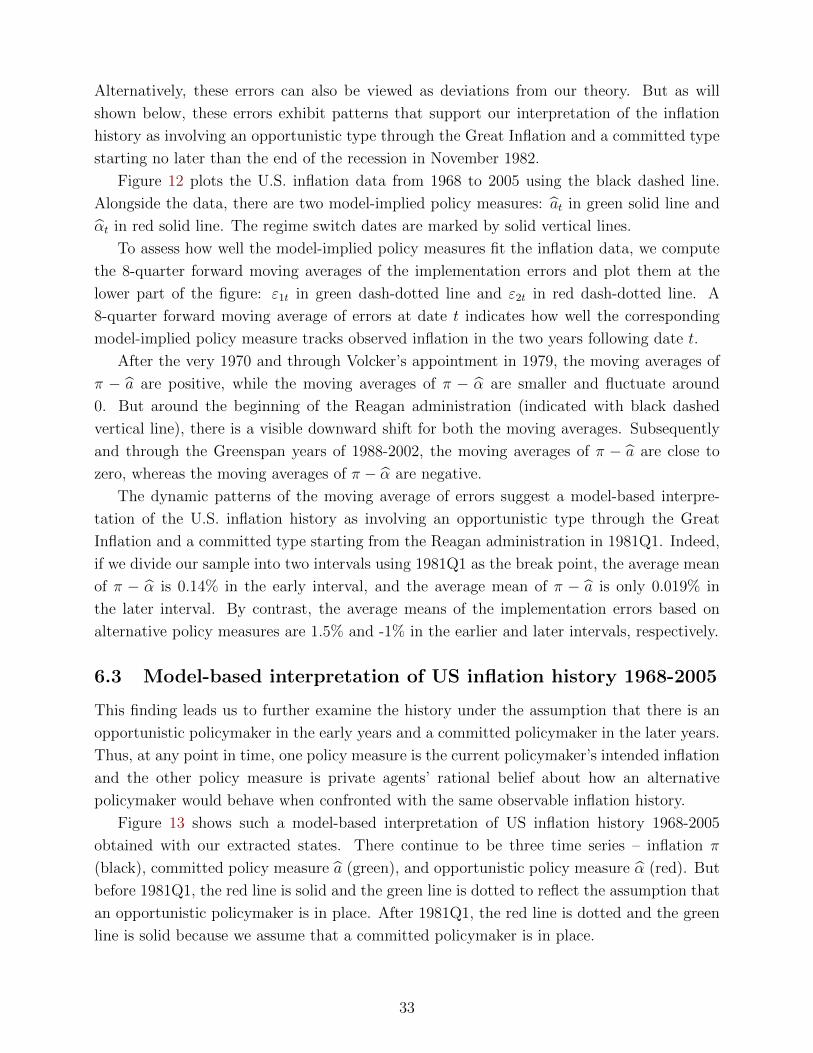
Alternatively, these errors can also be viewed as deviations from our theory. But as will

shown below, these errors exhibit patterns that support our interpretation of the inflation

history as involving an opportunistic type through the Great Inflation and a committed type

starting no later than the end of the recession in November 1982.

Figure 12 plots the U.S. inflation data from 1968 to 2005 using the black dashed line.

Alongside the data, there are two model-implied policy measures: at in green solid line and

αt in red solid line. The regime switch dates are marked by solid vertical lines.

To assess how well the model-implied policy measures fit the inflation data, we compute

the 8-quarter forward moving averages of the implementation errors and plot them at the

lower part of the figure: ε1t in green dash-dotted line and ε2t in red dash-dotted line. A

8-quarter forward moving average of errors at date t indicates how well the corresponding

model-implied policy measure tracks observed inflation in the two years following date t.

After the very 1970 and through Volcker’s appointment in 1979, the moving averages of

π − a are positive, while the moving averages of π − α are smaller and fluctuate around

0. But around the beginning of the Reagan administration (indicated with black dashed

vertical line), there is a visible downward shift for both the moving averages. Subsequently

and through the Greenspan years of 1988-2002, the moving averages of π − a are close to

zero, whereas the moving averages of π − α are negative.

The dynamic patterns of the moving average of errors suggest a model-based interpre-

tation of the U.S. inflation history as involving an opportunistic type through the Great

Inflation and a committed type starting from the Reagan administration in 1981Q1. Indeed,

if we divide our sample into two intervals using 1981Q1 as the break point, the average mean

of π − α is 0.14% in the early interval, and the average mean of π − a is only 0.019% in

the later interval. By contrast, the average means of the implementation errors based on

alternative policy measures are 1.5% and -1% in the earlier and later intervals, respectively.

6.3 Model-based interpretation of US inflation history 1968-2005

This finding leads us to further examine the history under the assumption that there is an

opportunistic policymaker in the early years and a committed policymaker in the later years.

Thus, at any point in time, one policy measure is the current policymaker’s intended inflation

and the other policy measure is private agents’ rational belief about how an alternative

policymaker would behave when confronted with the same observable inflation history.

Figure 13 shows such a model-based interpretation of US inflation history 1968-2005

obtained with our extracted states. There continue to be three time series – inflation π

(black), committed policy measure a (green), and opportunistic policy measure α (red). But

before 1981Q1, the red line is solid and the green line is dotted to reflect the assumption that

an opportunistic policymaker is in place. After 1981Q1, the red line is dotted and the green

line is solid because we assume that a committed policymaker is in place.

33

Figure 12: Inflation history and model-implied policy measures

Figure 13: Model-based interpretation of US inflation history

34

Besides the inflation measures, we also plot the SPF1Q forecast (blue), the extracted

cost-push shock ς (magenta), and the extracted reputation state ρ (cyan and measured on

the right hand axis).27

The Great Inflation is divided into four phases. From 1968 through 1972, both the op-

portunistic policy α and the shadow committed policy a are fairly stable between 3 and 4

percent and, since reputation is relatively high and stable at about .7, the SPF1Q closely

resembles the latter series. During 1973-4, a combination of cost-push shocks and deteri-

orating reputation occur and are reflected in the SPF1Q. The shadow commitment policy

rises along with these cost-push shocks, but less than the opportunistic policy. After this

episode, the SPF1Q is fairly stable in the 6% range during 1975-77, but the shadow com-

mitment policy is much lower and opportunistic policy much higher, with a policy gap δ of

about 2%. Reputation also stabilizes during this period, at about .4, a much lower level

than in early 1970s. Over the next few years, including the brief Miller regime of January

1978 through August 1979, the opportunistic policy rises again as a consequence of further

cost-push shocks. The shadow commitment policy rises even more because cost-push shocks

conjoin with the startup incentives for a new policymaker until it reaches the 7% range in

summer 1979. Reputation declines markedly to around .2 by mid 1979.28 This four-phase

pattern is consistent, in broad form, with the dynamics discussed in Section 5.

The Great Moderation starts with the end of the major recession in November 1982. From

this time and particularly during the Greenspan years of 1988-2005, inflation is well known

to be fairly stable and relatively low. Actual inflation roughly tracks the committed policy

a, even though our state variables were not designed to produce that result. The shadow

opportunistic policy α is also relatively low and stable during this period, but it nearly always

lies above actual inflation π and the committed policy a in keeping with the inflation bias of

ι = 0.5% per annum that is built into our model. Reputation rises steadily from around .4

in early 1983 to above .9 by the end of 2004.

The Volcker Disinflation. We previously argued that the 1968Q4-1979Q2 Great Inflation

period is best understood in terms of policy without commitment, while the 1982Q4-2005

Great Moderation period is best understood in terms of commitment. Between these dates,

of course, lies the famous Volcker disinflation.

After his appointment as chairman in August 1979, Paul Volcker quickly led the Fed

to introduce new operating procedures in October 1979, adopted – according to Lindsey et

al. (2004) – ”when the FOMC became convinced that its earlier gradualist strategy using

27We stress that our extracted reputation series ρt does not have two properties that one might think.First, it does not depend on observed inflation πt. Second, it does not involve the mechanical dependencebetween ρt and ρt+1 that one associates with Bayesian learning since ρt+1 = b(πt, a(st), α(st), ρt) would useobserved inflation πt and hence is not directly involved in the state construction.

28The Miller chairmanship begins in 1978Q1. The SPF1Q forecast changed little in this quarter relativeto the previous one (5.69% versus 5.77%) but the SPF3Q rose dramatically (to 6.56% versus 5.85%). In lateJanuary, Carter made a major speech on inflation, as reported by Clyde Farnsworth in the New York Times,“Carter Economic Message Asks Voluntary Price and Wage Brake,” 1/28/1978. Since then SPFQ3 fell in thefollowing quarter, while the SFPQ1 rose, our strategy extracts a large transitory movement in reputation.

35

finely tuned interest rate moves had proved inadequate for fighting inflation and reversing

inflation expectations.” Indeed, by March 1980, the Federal Funds rate had risen to 17.2%

from 11.4% in September 1979. However, with a sharp recession that started in early 1980

and was exacerbated by President Carter’s March 1980 program to reduce credit-financed

private spending, the Fed made an abrupt u-turn, so that the Federal Funds rate was back

to 11 percent in May 1980.29

Note that, in Figure 13, inflation during 1979 and 1980 lies between the model-implied

opportunistic policy α and committed policy a, perhaps more closely resembling the former.

The initial year of the Volcker chairmanship is frequently neglected in discussions of the Great

Disinflation, but is highlighted by our figures. The figure also features a decline in reputation

during the period, as a consequence of rising SPF inflation expectations. According to our

calculations illustrated in Figure 12, it is only in late 1980 or early 1981, that inflation starts

to become aligned with the commitment outcome.

Interestingly, although not designed to do so, this timing accords with the narrative of

Goodfriend and King (2005) who argue: “The true onset of the Volcker disinflation dates to

November 1980 or early 1981. In November, Reagan beat Carter in a landslide and brought

about a new course in U.S. economic policy. Among other things, the Reagan administration

voiced strong support for Fed monetary policy to reduce inflation.” But Orphanides (2005)

describes this as a “peculiar reinterpretation of history that pushes the ‘true’ onset of the

Volcker disinflation to November 1980 or later, a year and a half after Volcker’s appointment

as Chairman.”30

Yet disagreement on this front should not distract from points of agreement between

these authors and this study. First, during 1980, inflation rose rather than fell. Second,

during this year, inflation expectations rose (which Goodfriend and King (2005) capture

using longer-term interest rates, Orphanides (2005) captures using the SPF3Q, and Figure

13 captures using the SPF1Q). Third, starting in 1981, inflation expectations remained above

actual inflation with both declining over the course of the Great Disinflation, as Figure 1 in

Orphanides (2005) and Figure 13 stress. During the Volcker Disinflation, our extracted

reputation rises from a trough level of .1 in early 1981 to about .4 by the end of the recession

in November 1982. The process of gaining reputation is incomplete despite a close alignment

of actual inflation with the committed policy a, because declining inflation expectations also

lead to reductions in the opportunistic policy α, making it more difficult to determine the

type in place.

29Schreft (1990) describes the program in detail.30Orphanides (2005) criticizes the simplicity of the analysis in Goodfriend and King (2005) because it

assumes an exogenous path for credibility during the Volcker period. He argues “A better understandingof the interaction of economic shocks, policy and expectations formation in such an environment can beobtained by explicit modelling of the learning dynamics governing the evolution of inflation expectations.’Our paper supplies such an analysis.

36

6.3.1 Counterfactuals

We can also use our framework to perform historical decompositions of a and α into parts

attributable to each of the three states, (ς, ρ, µ). For the purpose of this study, we are

particularly interested in how the interplay between reputation state ρ and optimal policies

contributes to our model’s fitting to the observed inflation.

To this end, we perform a counterfactual exercise in this subsection that shuts down

the dynamics of reputation and compares the counterfactual policy measures with both the

original policy measures and the observed inflation.

In particular, we keep the cost-push shocks ςt and the pseudo-state variables µt the same

as the extracted states but set reputation state constant at a reference value ρ. We then

construct the counterfactual policies a(ςt, ρ, µt) and α(ςt, ρ, µt), together with the policy dif-

ference δ(ςt, ρ, µt) = a− α. We choose ρ = .6 since it is about the sample average of extract

reputation state ρt during 1968Q4-2004Q4.

Figure 14 shows the counterfactual policies (dash-dotted line) constructed using (ςt, ρ, µt),

along with the original policies (solid line) constructed using (ςt, ρt, µt) and the observed in-

flation (black line). The difference between counterfactual and original policies provides a

measure for the effect of time-varying reputation. The observed inflation serves as a bench-

mark that facilitates assessments on how much time variation in ρ helps our model to fit

data.

The top two panels in Figure 14 show the influence of time variation in ρ on a and α.

Between 1974Q1 and 1985Q4, the counterfactual policies lies below the original policies,

with the gap particularly large during the Great Inflation and the Volcker Disinflation. This

indicates that our model would completely miss the two important episodes of inflation

history if it wasn’t due to the dynamics of reputation, even when it is equipped with the same

price shocks and regime changes. If we move away from periods with large inflation swings

and into periods when the inflation is relatively stable, i.e., after 1990, the counterfactual

policies turn out to lie uniformly above the original policies, with the latter closer to the

observed inflation. Hence, our model would miss the Great Moderation too if reputation

were to fix at a historical average level.

The bottom panel in Figure 14 plots the policy difference (yellow lines) δ = a − α from

both the counterfactual (dash-dotted) and the original policies (solid). Comparing this panel

with the two panels above reveals that large gaps between the counterfactual and original

policies a and α are associated with large gaps between the counterfactual and original δ. In

other words, similar to our message in Section 5.4, the policy difference is a key choice of the

committed policymaker and is the key mechanism in our model which has relevance for the

U.S. inflation experience.

One may further inquire what drives the gaps between the counterfactual and original

δ. To answer that, we also plot the extracted reputation states ρ (cyan solid line) and its

historical average (cyan dotted line) measured on the right hand axis. Notice that when

37

the extracted reputation states are below its historical average, i.e., between 1974Q1 and

1985Q4, the counterfactual δ is above the original δ. This captures the quantitatively im-

portant reputation-building effects when reputation is relatively low. On the other hand,

when the extracted reputation states are above its historical average, i.e., after 1990, the

counterfactual δ lies above the original δ. That is, there are quantitatively important effects

of accommodating imperfect credibility when reputation is relatively high.

In sum, the results of the counterfactual exercise highlight the quantitative importance

of the dynamics interplay between private sector’s belief (reputation) and the optimal policy

choices by the two types (δ) in aligning our model-implied policies with the historical inflation

data.

7 Conclusions and Final Remarks

In this paper, we study optimal monetary policy in setting where the private sector is

forwarding-looking and learning about the type of policymaker in place. The policymaker can

be either a patient and committed type, or an impatient and opportunistic type that cannot

commit. Being able to commit or not, the policymaker in place chooses inflation policies

optimally, taking into account the learning and rational expectation of the private sector.

To solve the model, we adopt a mechanism design approach so that the equilibrium can be

obtained as the solution to a recursive optimization of the committed policymaker. In partic-

ular, we view the committed type as choosing its action and the action of the opportunistic

type subject to an incentive compatibility constraint. The relevant incentive compatibility

constraint is an unusual one because it involves the beliefs of a third party, i.e., the private

sector. Numerical exercises using our calibrated model demonstrate a striking success of this

simple theory in explaining the U.S. inflation history from 1969 to 2005.

In our setup, introducing an aggregate demand side (an IS curve and a Fisher equation)

will allow us to determine the short-term nominal interest rate as a function of the model’s

state variables. Coupling this with a term structure theory will allow us to determine the

long-term nominal rate. We are particularly interested in understanding how private sector

learning and time-varying reputation affect the long-term rate, as it is frequently used as

an indicator of long-term expected inflation and policymaker reputation. This would be a

valuable future extension of the current work.

Another interesting extension of our current work is to allow for a patient opportunistic

type. To do so, one needs to modify the recursive optimization of the committed type

to incorporate the promised value for the opportunistic type in the incentive compatibility

constraint. This will significantly complicate the computation. We leave this extension to

future work.

38

Figure 14: Counterfactual with ρ constant at history average level.

39

References

Atkeson, Andrew and Patrick J. Kehoe, “The advantage of transparency in monetarypolicy instruments,” Federal Reserve Bank of Minneapolis Staff Report 297, 2006.

Backus, David A. and John Driffill, “Inflation and Reputation.,” American EconomicReview, 1985, 75(3), 530–538.

Backus, David and John Driffill, “Rational Expectations and Policy Credibility Followinga Change in Regime,” The Review of Economic Studies, April 1985, 52 (2), 211–221.

Barro, Robert J., “Reputation in a model of monetary policy with incomplete informa-tion,” Journal of Monetary Economics, January 1986, 17 (1), 3–20.

Brayton, Flint, Thomas Laubach, and David Reifschneider and, “Optimal-ControlMonetary Policy in the FRB/US Model,” FEDS Notes, nov 2014, 2014 (0035).

Chang, Roberto, “Credible Monetary Policy in an Infinite Horizon Model: Recursive Ap-proaches,” Journal of Economic Theory, 1998, 81, 431 – 461.

Cukierman, Alex and Allan H. Meltzer, “A Theory of Ambiguity, Credibility, andInflation under Discretion and Asymmetric Information,” Econometrica, sep 1986, 54 (5),1099.

and Nissan Liviatan, “Optimal accommodation by strong policymakers under incom-plete information,” Journal of Monetary Economics, feb 1991, 27 (1), 99–127.

Debortoli, Davide, Junior Maih, and Ricardo Nunes, “Loose commitment in media-scale macroeconomic models: theory and applications,” Macroeconomic Dynamics, aug2012, 18 (01), 175–198.

Dovis, Alessandro and Rishabh Kirpalani, “Rules without Commitment: Reputationand Incentives,” Working paper, 2019.

Eusepi, Stefano and Bruce Preston, “The Science of Monetary Policy: An ImperfectKnowledge Perspective,” Journal of Economic Literature, mar 2018, 56 (1), 3–59.

Evans, George W. and Seppo Honkapohja, “Adaptive Learning and Monetary PolicyDesign,” Journal of Money, Credit and Banking, 2003, 35 (6), 1045–1072.

and , “Expectations, Learning, And Monetary Policy: An Overview Of Recent Re-search,” Working Papers Central Bank of Chile 501, Central Bank of Chile October 2008.

Faust, Jon and Lars E. O. Svensson, “Transparency and Credibility: Monetary Policywith Unobservable Goals,” International Economic Review, 2001, 42 (2), 369–397.

Gali, Jordi, Monetary Policy, Inflation, and the Business Cycle, Princeton Univers. Press,2015.

Golosov, M., A. Tsyvinski, and N. Werquin, “Recursive Contracts and EndogenouslyIncomplete Markets,” in “Handbook of Macroeconomics,” Elsevier, 2016, pp. 725–841.

Goodfriend, Marvin and Robert G. King, “The incredible Volcker disinflation,” Journalof Monetary Economics, jul 2005, 52 (5), 981–1015.

40

Gordon, Robert J. and Stephen R. King, “The Output Cost of Disinflation in Tradi-tional and Vector Autoregressive Models,” Brookings Papers on Economic Activity, 1982,1982 (1), 205.

Hansen, Stephen and Michael McMahon, “First Impressions Matter: Signalling as aSource of Policy Dynamics,” The Review of Economic Studies, feb 2016, 83 (4), 1645–1672.

Khan, Aubhik, Robert G. King, and Alexander L. Wolman, “Optimal MonetaryPolicy,” Review of Economic Studies, oct 2003, 70 (4), 825–860.

King, Robert G., Yang K. Lu, and Ernesto S. Pasten, “Managing Expectations,”Journal of Money, Credit and Banking, dec 2008, 40 (8), 1625–1666.

Kydland, Finn E. and Edward C. Prescott, “Dynamic optimal taxation, rational ex-pectations and optimal control,” Journal of Economic Dynamics and Control, jan 1980, 2,79–91.

Lindsey, David E., Athanasios Orphanides, and Robert H. Rasche, “The Reformof October 1979: How It Happened and Why,” Technical Report 2004.

Lu, Yang K., “Optimal policy with credibility concerns,” Journal of Economic Theory, sep2013, 148 (5), 2007–2032.

, Robert G. King, and Ernesto Pasten, “Optimal reputation building in the NewKeynesian model,” Journal of Monetary Economics, dec 2016, 84, 233–249.

Mailath, George J. and Larry Samuelson, Repeated Games and Reputations: Long-runRelationships, Oxford University Press, 2006.

Marcet, Albert and Ramon Marimon, “Recursive Contracts,” Econometrica, 2019, 87(5), 1589–1631.

Matthes, Christian, “Figuring Out the Fed-Beliefs about Policymakers and Gains fromTransparency,” Journal of Money, Credit and Banking, jan 2015, 47 (1), 1–29.

Mishkin, Frederic S. and Klaus Schmidt-Hebbel, “Does Inflation Targeting Make aDifference?,” NBER Working Papers 12876, National Bureau of Economic Research, IncJanuary 2007.

Orphanides, Athanasios, “Comment on: “The incredible Volcker disinflation”,” Journalof Monetary Economics, jul 2005, 52 (5), 1017–1023.

and John C. Williams, “Monetary Policy Mistakes and the Evolution of Inflation Ex-pectations,” in “The Great Inflation: The Rebirth of Modern Central Banking,” Universityof Chicago Press, June 2013.

Phelan, Christopher and Ennio Stacchetti, “Sequential Equilibria in a Ramsey TaxModel,” Econometrica, 2001, 69 (6), 1491–1518.

Roberds, William, “Models of Policy under Stochastic Replanning,” International Eco-nomic Review, oct 1987, 28 (3), 731.

Roger, Scott and Mark R. Stone, “On Target? the International Experience with Achiev-ing Inflation Targets,” IMF Working Paper No. 05/163, 2005.

41

Schaumburg, Ernst and Andrea Tambalotti, “An investigation of the gains from com-mitment in monetary policy,” Journal of Monetary Economics, 2007, 54 (2), 302–324.

Schreft, Stacey L., “Credit controls: 1980,” Economic Review, 1990, 76 (Nov), 25–55.

Walsh, Carl E., Monetary Theory and Policy, MIT Press Ltd, 2010.

Watson, Mark W., “Inflation Persistence, the NAIRU, and the Great Recession,” AmericanEconomic Review, may 2014, 104 (5), 31–36.

Woodford, Michael, “Optimal Interest-Rate Smoothing,” The Review of Economic Stud-ies, 2003, 70 (4), 861–886.

, “Macroeconomic Analysis Without the Rational Expectations Hypothesis,” Annual Re-view of Economics, aug 2013, 5 (1), 303–346.

Xandri, Juan Pablo, “Credible Reforms: A Robust Implementation Approach,” Workingpaper, 2017.

42