Managing

clearinghouse risk

for NDF cleared

contracts Validating the HS/VaR method for NDF FX CCP Clearing risk

Johan Olsson 2015

1

Abstract

In this thesis we describe and discuss the reality for a central clearing party clearinghouse.

The importance of sound risk management is discussed. We specifically validate the usage of

a Historical Simulation/VaR approach for managing the risk when acting as a CCP for the

Non Delivery Forward FX instrument. The method is back tested and some alternative

approaches are proposed.

2

Acknowledgement

I would like to thank Filip Lindskog at Department of Mathematical Statistics at the Royal

Institute of Technology (KTH) for his guidance and valuable remarks.

I would also like to thank David Karlgren at NASDAQ who helped me retrieve and

understand valuable data in the relevant field.

Finally I would like to thank my wife Jeanette Harrysson for her understanding and for taking

care of the family while I have been working weekends and holidays with this thesis.

3

Introduction

Since the financial crisis in 2008 regulators are pushing OTC non-regulated trades to be

cleared on a Central Counterpart (CCP) facility. The purpose is to lower the counterparty risk

and avoid contagion if a large financial institute (like Lehman Brothers) defaults. A study on

how the bilateral trading in combination with default (in form of Credit Default Swap

instruments) had an impact on how the credit crises became worse is given in [ref 7].

A CCP transform the risk from the bilateral counterparty risk to a risk towards the CCP itself.

The CCPs is a risk sharing arrangement where each clearing member is providing coverage

for the risks that they introduce in a shared default fund. In [ref 1] it is shown how the

introduction of a CCP reduces liquidation and shortfall losses for the banks but it introduces

tail risk which can lead to higher systemic risk [ref 13]. Systemic risk is related to how a

financial network is arranged and a general analysis on how systemic risk spreads in a

financial network can be found in [ref 9, 10]. The effect of a default of a CCP is large and

three historical actual cases are described in [ref 2]. It is therefore of high importance that the

CCP have control of the risks it carries. Especially of importance is to have control of the tail

risk since this is what historically has shown to be where contagion and wrong way risk is

exposed. Wrong way risk is that the default of members is more likely when the market is in

stress and the portfolio is of low value. Contagion refers to that the member default itself

gives rise to more stress in the market. Descriptions and studies of contagion in financial

networks can be found in [ref 4, 5, 6 and 8]

For the purpose of measuring and managing the risk it is important that the CCP uses methods

that take care of the tail risk to avoid a contagion effect. Different methods of quantifying

risk measures are studied in [ref 3]. One popular quantitative measure is to use a VaR based

approach. This is therefore also what the regulators are approving as risk measure for new

OTC markets that needs to be cleared on a CCP.

For the various clearinghouses in Europe that now gets the approval of clearing FX

instruments (NASDAQ and London Clearinghouse so far) are both relying on VaR. On

London Clearinghouse a margin method named PAIRS is used. PAIRS is an expected

shortfall value-at-risk (VaR) model based on filtered historical simulation incorporating

volatility scaling [ref 11]. NASDAQ Clearing is using a VaR based on Historical Simulation

[ref 12].

In this study a back test of the VaR based on Historical Simulation margin methodology is

done for FX NDF instruments. The aim is to validate this model to capture the clearinghouse

counterparty risk that NASDAQ have for these instrument.

The paper start by describing briefly the credit crisis events in 2008 and the European

regulations stating that OTC products should be cleared through a CCP is formed. A more

thorough description of what a Clearinghouse is and how it is managed is provided. Then a

brief description of the instruments in the FX market in general and Non Delivery Forwards in

particular is given. VaR based on Historical Simulation is described and then a numerical

4

back testing is done to state the models accuracy. We end with a conclusion on how the model

will perform in a stressed scenario where a risk of contagion and systemic risk materialize.

5

The 2008 Credit Crisis In 2008 a financial there was a financial crisis that affected practically the whole world. The

background was that a number of banks traded mortgage backed securities that was in reality

not possible to value correctly. The securities that was traded were built up of a number of

high risk mortgages (subprime loans). The financial actors that were selling them (loan

institutes) argued and showed that the risk for a portfolio of these high risk mortgages was

low due to that the house prices will continue to rise. This argument was based on historical

simulation. Historically house prices have not fallen but always been raising. The US

government had also been stimulating and controlling the house market with a number of

decisions throughout the years before. The decisions all have been aiming at seeing to that

everybody could own a house. Therefore directives for loan institutes like Freddie Mac and

Fannie May was given by the government to give a substantial amount of house loans to

people with less credit abilities. To not have the full risk of all these high risk loans the loan

institutes started to construct Credit Default Swaps which is financial papers where the credit

risk is swapped to the counterpart for a premium. These financial papers where traded over

the counter which means that they were not regulated by any third party. The buyers of the

CDS were investment banks such as Lehman Brothers.

One effect of the credit crisis was that one of the largest investment banks, Lehman Brothers,

defaulted resulting in a financial mess that has many years after not been settled. Lehman

Brothers held numerous open positions with other financial actors. These open positions were

not settled and hence a number of financial actors lost their money. The counterparty risk,

which the most of the actors thought of as very low when Lehman Brothers was the

counterparty, had actually materialized. Since this had effect on the whole society the

governments around the world understood that they need to do create some mechanisms that

hinder this from happen again.

Regulations

European Markets Infrastructure Regulation (EMIR)

As a consequence of the 2008 financial crisis the G20 organization decided in September

2009 that the risks in the financial markets needed to be regulated more thoroughly. More

specifically a conclusion was made that the OTC traded derivative contracts needed to be

traded on an exchange or another electronic trading platform. The contracts also need to be

cleared on a central counterparty (CCP) where it is possible. The OTC derivative contracts

should also be reported to a central Trade Repository (TR) to keep track of all the financial

contracts that were traded.

Each part in the G20 got the assignment to work out regulations based on the agreement made

by G20. In USA the agreement was implemented through the Dodd-Frank legislation. In EU a

similar legislation was presented in 2010 called European Market Infrastructure Regulation

(EMIR). The part of the agreement that OTC derivative contracts are to be traded on

exchange or another electronic trading platform is regulated in MiFID II.

6

The legislation directive is divided in four areas:

1. The OTC derivatives has to be cleared on a CCP

2. How OTC contracts that is not obliged to be cleared on CCP shall be handled

3. Reporting of OTC trades to a central TR

4. Authorization, rules and regulation of CCP and TR

There have later been small changes to how the legislation will be implemented. One example

is that all derivatives contracts and not just the OTC derivatives contracts be reported to a

central TR. The details of the legislation are being agreed and a number of so called technical

standards are being constructed. Two examples that yet have to be decided is (i) how to

handle OTC derivatives that is not obliged to be cleared through a CCP and (ii) which OTC

derivative contracts that shall be obliged to be cleared through a central CCP.

Clearing of OTC contracts through a CCP

To be able to clear an OTC contract the CCP needs to be able to manage the risk that clearing of this specific OTC contracts means. The OTC contracts are all quite specific in how they are constructed and hence the risk is not always possible to manage within the existing mechanisms on the CCP. Therefore it is not always possible to clear an OTC contract on a CCP just because it is possible to clear the contract as such. To decide which OTC contracts that can be cleared the legislation is including two different approaches, “bottom up” and “top down”. In the “bottom up” approach an OTC derivatives contract is decided to be included in the obligation to be cleared on CCP list when a CCP decides that it can clear that contract. The local financial authority (“FinansInspektionen” in Sweden) is giving the permission for the CCP that it can clear the OTC derivative instrument when the CCP have passed an audit of the clearing and risk mechanisms for the new instrument. The local authority is notifying ESMA (European Securities and Markets Authority) who in turn is creating a technical standard for clearing of the OTC derivative contract. The technical standard is approved by the commission and then the specific OTC derivative contract is part of the obligation to be cleared on CCP list. The “top down” approach means that ESMA together with European Systemic Risk Board (ESRB) is deciding which OTC derivatives contract that should have a demand to be cleared through a CCP. The list of which OTC derivatives class that is currently possible to be cleared on an approved CCP is managed by ESMA. The list of authorized derivatives classes and CCP’s are available on at ESMA’s web site [ref 19]. There is one instrument in the FX asset class that is for the moment part of the list of authorized (but not obliged) cleared OTC products, namely the Non Delivery Forward (NDF). We will look closer on this instrument later in this report. All financial counterparties are part of the obligation to clear the OTC derivatives trades on a CCP. As Financial counterpart is typically banks, broker firms and fund companies accounted for. Non-financial companies are obliged to clear the trades in the OTC derivatives contracts first after they have a total position that is above a certain clearing threshold. When the total position is valuated the trades that are risk mitigating positions is not included.

OTC Contracts that are not obliged to be cleared through CCP

In the cases where financial and non-financial counterparties that are above the clearing threshold is part of a OTC derivatives contract trade that is not part of the obligated CCP cleared list procedures for measure, watch and minimizing the operational and credit risks

7

needs to be in place. The procedures are for example to confirm the terms of the contract within a certain time frame and exchange of collaterals or capital.

Reporting of trades to central TR

All counterparts are obliged to report all derivatives contracts that they have made in to a central trade repository. They also need to report all changes or terminations that are made to the contracts. The reporting needs to be done on the next bank day after such contract have been made.

Authorization, supervision and rules for CCP and central TR

The local authorities (FI in Sweden) are handling the authorization and supervision for the CCP’s. The local authority takes the decision in conjunction with ESMA and other authorities that are supervising the largest clearing counterparties. EMIR went into effect on August 16 2012 and is directly applicable in all member states. The technical standards are being constructed and Swedish complementing laws have been implemented [ref 14, 15, 16, 17].

Clearinghouse

When a trade between two parties is made in a trading system or over the counter this trade is

bilateral. The parties that are part of this trade have a risk that the counterparty will default or

for some other reason not be able to fulfill their commitment. This risk is referred to as

counterparty risk. This risk can be cumbersome to handle for a lot of actors in the financial

industry and could therefore act limiting on the number of deals they are willing to do. This

has an effect on the market to become less liquid and of higher risk. To remove this risk from

the trading parties they can clear the trade on a Central Counter Party (CCP). It is typically a

Clearinghouse that acts as a CCP for the market. The clearinghouse transforms the bilateral

trade to become a Cleared Trade instead. A cleared trade is in reality two trades with the

Clearinghouse. One of the trades is with counterparty A and the other trade is a reverse trade

with counterparty B.

For example if Trading firm A buys 200 CompanyXY stocks from Trading firm B and clears

this trade with the CCP Clearinghouse the bilateral trade transforms to one trade where the

CCP sell 200 CompanyXY stocks to Trading firm A and one trade where the CCP buys 200

CompanyXY stocks from Trading firm B.

Bilateral Trade: A��B

Cleared Trade: A��CCP, CCP��B

In this way the counterparty risk is transferred to the clearinghouse. The clearinghouse does

however not has any market risk since the different deals that makes up the full trade are

offsetting each other’s market risk. The counterparty risk is in effect until the trade has been

settled. It normally takes three days for an exchange traded deal to be settled. To be settled

means that assets and money have been transferred between the trade counterparties

respective accounts according to the deal that was made. A deal can however mean that a

8

position is open and not settled for much longer period than three days as well. A lot of

derivatives is open and not settled for the lifespan of the contract.

The CCP clearinghouse needs to manage the counterparty default risk during the settlement

period. The clearinghouse manages this by calculating the risk and requires the counterparties

to post collaterals that cover the risk margin requirements that the clearinghouse needs to

cover the unsettled positions that the counterparty have.

Operate a CCP Clearinghouse

Receive trades

The clearinghouse needs to be effective in receiving trades. It needs to be able to interpret and

categorize trades from different markets. Trades that origin from regulated markets such as

the normal Equity Derivatives market is often quite straight forward to interpret and receive.

The trades that is received from non-regulated markets where the trading is done OTC can

involve a lot of parameters that otherwise is standardized.

Manage prices

To be able to calculate the risks and evaluate the posted collaterals it is of outmost importance

that the clearinghouse has a correct view of the market at any given time. The base for this

knowledge is to have prices of good quality for all markets where the clearinghouse is able to

clear trades on. For many instruments that are not fully liquid the clearinghouse cannot get

real prices from the market. In these cases it needs to correlate to other market prices and

derive prices from the real prices on that market.

Manage Risk

The clearinghouse needs to be as risk neutral as possible at each given time. To be able to be

risk neutral the clearinghouse relies on quantitative risk calculations for the different

counterparty risks to set how much collaterals it needs to request from the members to cover

for the risk. There are different measures included in managing the risk. First of all the

clearinghouse needs to calculate the Risk Margin that the parties need to post as collaterals

continuously. The margin is a collateral value that covers a part of the credit risk that the

clearinghouse have in the outstanding trade. The margins are then combined for the whole

portfolio that the member has outstanding on the clearinghouse. The result is the total margin

that the member has to cover with posted collaterals. If the member is in deficit, meaning

have not enough collateral posted to cover the margin requested by the clearinghouse, the

clearinghouse will do a margin call. In this case the member has a certain time to post

collaterals to cover the margin requirement and go out of deficit. If the member is in surplus,

meaning have posted more collateral than is required as margin, the clearinghouse gives back

the amount in collateral that is above the margin needed. There are a number of different

margin components that are listed below

9

Initial Margin

Start margin that is required to be so collateralized that the member can be allowed to have a

clearing account on the CCP clearinghouse.

Maintenance margin requirement

Base margin required to be posted to the clearinghouse to be able to hold an open position.

The margin requirement is calculated by using different quantitative margin methodologies.

Mark to market (MTM) aka variation margin

Cash stream to/from the member that holds the position of a Future. The main purpose of a

variation margin is to balance the potential loss of the day due to a certain futures position

held in the market.

Premium Margin

The member that has an outstanding Option needs to provide a margin to secure a buy-back of

the option.

Additional Margin

A scenario based calculated extra margin requirement. The purpose is to cover for a very bad

scenario. The clearinghouse calculates different stressed scenarios continuously to calculate if

the requested margin is covering for extreme scenarios or if additional margin is needed.

Calculating Margin

To cover for the different markets the clearinghouse uses different kind of margin methods to

calculate the margin requirement for the members’ positions. Since the different underlying

and financial instruments have different features there is a need to use different methods. The

methods all have in common that statistical methods are used. On NASDAQ clearing in

Stockholm the following methods are used for the different markets; OMS II for Equity

derivatives, Cash Flow Margin for fixed income markets and a modified SPAN method is

used for the commodities markets.

Manage Collaterals

Collateral is something of monetary value, for example a stock, cash or certificates. The

collaterals are posted from the parties to cover the requirements from the clearinghouse to

cover the margin requested. The clearinghouse needs to constantly know the value of the

collateral to be able to see to that the margin requirement is covered. It does that by constantly

finding the fair value of the assets posted as collaterals. In the case of the assets being cash it

is fairly straight forward. However the cash could be posted in a currency that is not the base

currency used by the clearinghouse. In that case the cash needs to be checked towards the

current exchange rates to find the fair value of the collateral. When it comes to other securities

such as stocks and certificates the clearinghouse constantly value the collaterals and compares

to the calculated margin requirement.

10

Settlement

The clearinghouse creates settlement reports for the banks that hold the assets that will change

owners from different trades. The banks will act upon the settlement reports and move assets

accordingly.

Default management

If a member of the clearinghouse is considered to go into default the clearinghouse will act to

ensure the commitments towards other members. There are a number of measures that the

clearinghouse is entitled to take. One key factor for the success of the default management is

that the clearinghouse is acting quickly and that it has control of the members’ outstanding

trades and its collaterals. A back-up member is always decided for each member. When a

member goes into default the clearinghouse will move the assets to the back-up member. The

back-up member will then hold the positions of the defaulting member.

To cover for different default scenarios the Clearinghouse holds Clearing capital. The first

layer of such Clearing Capital is the margin posted by the member. After that there are

different layers of capital that is available. Some layers are the Clearinghouse own capital and

some layers are capital provided by the members. All the layers of capital and the rules of

how they are constructed and used are called “the clearinghouse waterfall”.

As part of the risk management on the Clearinghouse the Clearinghouse calculates the amount

of Clearing capital that is on risk daily to calibrate the amount posted. This is done by setting

up a number of extreme scenarios that should cover that the top three largest members should

default in different scenarios.

11

FX market The Foreign Exchange (FX) market is the market where the exchange rates spot product and

derivative products on exchange rates are traded.

There are a number of specific products that packages the FX market. They are traded OTC

and is not cleared on a clearinghouse today. They all have in common that they rely on the

“fixing”. The fixing is an agreed value of a currency towards base currency.

Non Deliverable Rolling Spot contracts (“NDRS”)

The Non Deliverable Rolling Spot contract is just like a spot contract but there is never a delivery of the actual asset. The parties are instead closing out the contract by an opposite trade alternatively the P/L is settled and the contract is rolled to the next date. The contract is very similar to a future from a risk measuring perspective.

Non Deliverable Forward contracts (“NDF”) detailed

A Non-Deliverable Forward (NDF) transaction is an FX Forward hedging mechanism where the physical exchange of currency at expiry is replaced by settlement between counterparties of the net profit/loss on the contract calculated using the prevailing Spot Fixing Rate two days prior to settlement (cash settled forward). The net settlement will occur in a predetermined convertible currency, typically USD. A trade involves two currencies based on a FX spot rate and forward points. The points will reflect the interest rate differential between the two currencies. The NDF is often used in currencies when there are currency controls or restriction. NDF’s can be quoted in standard tenors (length of a contract) as well as odd dates up to one year but quotes are sometimes also up to 2 years on request. The most commonly traded NDF tenors are IMM dates (International Monetary Market dates). NDFs are typically quoted with the USD as a base currency and cash settled in US dollars, i.e. it’s settled in the base currency. The list below shows example of currency pairs that are part of scope for being cleared on a CCP.

Currency pair Trade currency

USDARS Argentine peso

USDBRL Brazilian real

USDCLP Chile peso

USDCNY China yuan renminbi

USDCOP Colombia peso

USDINR India rupie

USDIDR Indonesian rupie

USDKRW South Korean won

USDMYR Malaysia ringgit

12

USDPHP Phillipin peso

USDRUB Russia rubel

USDTWD Taiwan dollar

Example: Assume a market with 2 participants {A, D}. D is entering a business agreement in Indonesia where a payment in Indonesian rupies will be given to D in TD days. The fixing rate between USD and IDR is on the day of the contract F. To hedge the position from changes in FX rates between USD and IDR D enters an OTC NDF contract in USDIDR with market participant A with N notional amount (USD). This means a forward agreement where D buys N USD and sell N*F amount IDR. On the fixing date, when the fix rate is S, D sells N*S amount of the IDR and receives N amount of USD. For the contract he P/L for D becomes:

�/� = (� ∙ � − � ∙ )/� To clear this contract on a CCP the trade is confirmed in a trading venue and sent to the CCP. The CCP then takes on the responsibility towards A and D respectively that the agreement is fulfilled even if A or D goes into default or similar credit risk is materialized during the period of the contract. To understand the risk inherited that the CCP is having when it holds NDF positions we need to now the market value of the NDF at each given time. Since there is no liquid market for NDF it has to be valued from prices in other liquid markets that are correlated with NDF market.

Calculations

The definitions below are used for the calculations.

X Trade currency. For example IDR in an USDIDR NDF agreement.

Y Base currency. To which currency the Trade currency should be compared towards. Typically USD

Z Settlement currency. The currency in which the settlement should be done. For example USD.

Nx Notional amount in currency X, this is the “face value” of the NDF, which is agreed between the two counterparties. Note that this notional amount will not be exchanged in any of the currencies since the contract is settled without delivery

TF Fixing date. The time whereby the comparison between the contracted NDF exchange rate and the market exchange rate is made.

FNDF(X,Y) Contracted NDF exchange rate from currency X to currency Y. This rate is agreed on the transaction date.

FFix(X,Y) Fixing spot exchange rate from currency X to currency Y. This exchange rate is given by an agreed exchange rate distributor. In the NDF market Reuters is the agreed distributor of fixing exchange rates.

TS Settlement date. The date when the difference between the contracted NDF rate and the market rate is paid or received in currency Z.

13

TF The fixing date. When the fixing rate that the contract should be settled in are decided. Typically 3 days before TS.

When entering a NDF agreement contract the details that are given by the parties are: NX,TF, FNDF(X, Y), X, Y and Z.

Settlement calculations

At cash settlement all the values are calculated in the cash settlement currency Z. The long and short legs are valued separately according to Long leg: �� ∙ ��(�, �) Short leg: �� ∙ �� (�, �) ∙ ��(�, �) Settlement amount is the difference between the long and short leg and is settled in currency Z.

�� ∙ ��(�, �) − �� ∙ �� (�, �) ∙ ��(�, �) = = ��( ��(�, �) − �� (�, �) ∙ ��(�, �)) Example of a settlement calculation

Customer D: Buy IDR / Sell USD Notional 1M IDR, cash settled in USD Contracted NDF rate: 0.000077778 At expiry the spot exchange rate between IDR and USD is 0.000081112 which lead to the following calculation:

���� = 1000000 �� (���, ���) = 0.000077778 ��(���, ���) = 0.000081112 If this was a deliverable forward the customer was to get IDR and deliver USD according to:

��� = 1000000 ��� = 1000000 ∙ 0.000077778 = 77.8 In this forward a cash settlement will be done in USD so the IDR part will be exchanged to USD using the official spot rate. Long: �� ∙ ��(�, �) = ���� ∙ ��(���, ���) = 1000000 ∙ 0.000081112 = 81 Short: �� ∙ �� (�, �) ∙ ��(�, �) = ���� ∙ �� (���, ���) ∙ ��(���, ���) =1000000 ∙ 0.000077778 ∙ 1 = 77.8 This implies that �/� = 81 − 77.8 = 3.2 Hence the customer has to pay $3.2 in cash at settlement date. :::::

14

Market value calculation

For a position at settlement the market value is trivial since it is the settlement amount. But prior to this the market value has to be calculated.

Position: �� , # , �� (�, �), �$%&', �()%*+, �

At cash settlement all cash flows are transferred in the cash settlement currency Z. This would then be the market value at time TF. To calculate the market value at a previous time t, the forward rate for the different currencies must be calculated.

,-(.) = /(�, ., #0) ∙ �� ∙ [ ��(�, �, ., # ) − �� (�, �) ∙ ��(�, �, ., # )] Where

MV(t) The market value calculated at time t.

D(Z,t,TS) Discount function to discount from the settlement date TS back to the valuation date t for currency Z.

FFix(X,Z,t,TF) The fixing value at time TF for the currency pair X and Y estimated at t.

Since there seldom is information about the currency forward curve and discount function for each currency it is more convenient to use the interest rates, or discount factors, in respective currencies.

/(�, ., #) = 34*5(64+) (�, �, ., .) = �(�, �, .) (�, �, ., #) = �(�, �, .) ∙ 3(*74*8)(64+) [ref 18]

S(X,Y,t) Spot exchange rate at time t for converting currency X to Y.

9� Risk free interest rate (continuously compounded interest rate per annum) annually for currency X.

Rewriting the equation for MV previously defined:

,-(.) = /(�, ., #0) ∙ �� ∙ [ ��(�, �, ., # ) − �� (�, �) ∙ ��(�, �, ., # )] =

= 34*5(6:4+) ∙ �� ∙ ;�(�, �, .) ∙ 3(*54*8)(6<4+) − �� (�, �) ∙ �(�, �, .) ∙ 3(*54*7)(6<4+)= =

= 34*5(6:4+) ∙ �� ∙ 34*5(6<4+) ∙ ;�(�, �, .) ∙ 34*8(6<4+) − �� (�, �) ∙ �(�, �, .) ∙ 34*7(6<4+)= =>

,-(.) = �� ∙ 34*5(6:46<) ∙ ;�(�, �, .) ∙ 34*8(6<4+) − �� (�, �) ∙ �(�, �, .) ∙ 34*7(6<4+)= With discount factors:

,-(.) = /(�, # , #0) ∙ �� ∙ [�(�, �, .) ∙ /(�, ., # ) − �� (�, �) ∙ �(�, �, .) ∙ /(�, ., # )] Hence both discount functions and currency forward functions can be used to calculate market value for NDF instruments. Focus will be on discount functions.

15

Example on market value calculations

Customer D: Buy SEK / Sell USD Notional 1M SEK, cash settled in USD Contracted NDF rate: 0.1211 Valuation date: 2015-05-05 Fixing date: 2015-08-04 Settlement date: 2015-08-07 X: SEK, Y: USD, Z: USD NSEK = 1 000 000 FNDF(SEK, USD) = 0.1211 Information from market data sources can give a discount function in USD and SEK or the underlying instruments can be used to construct such function. It is therefore assumed that a discount function for each currency is available in the pricing process.

/(�>?, ., # ) = /(�>?, 150505,150804) = 0.9755 /(�>?, ., #0) = /(�>?, 150505,150807) = 0.9752 /(���, ., # ) = /(���, 150505,150804) = 0.9989 /(���, ., #0) = /(���, 150505,150807) = 0.9987

/(���, # , #0) = /(���, ., #0)/(���, ., # ) =

/(���, 150505,150807)/(���, 150505,150804) =

0.99870.9989 = 0.9998

Spot rates are available in the market:

�(�>?,���, .) = �(�>?,���, 150505) = 0.1123 �(���, ���, .) = 1 Hence the market value is given by the use of the previously defined equation:

,-(.) = /(�, # , #0) ∙ �� ∙ [�(�, �, .) ∙ /(�, ., # ) − �� (�, �) ∙ �(�, �, .) ∙ /(�, ., # )]

,-(150505) = /(���, 150804,150807) ∙ 1000000∙ [�(�>?,���, 150505) ∙ /(�>?, 150505,150804) − �� (�>?, ���)∙ �(���, ���, 150505) ∙ /(���, 150505,150804)]

,-(150505) = 0.9998 ∙ 1000000 ∙ [0.1123 ∙ 0.9755 − 0.1211 ∙ 1 ∙ 0.9989] = −11395 The calculated market value of the position is -11 395 USD. Note:

• The discount factor between settlement and fixing date has probably a so low impact that it is not relevant for calculating risk.

Non Deliverable option (“NDO”)

The NDO contract is a European style option which is valuated with the Garman–Kohlhagens option pricing formula which is very similar to the Black & Scholes & Merton formula and the inputs are almost identical. At the end of the contract the P/L is settled in the base currency, which often is USD, instead of in the two currencies being traded in the legs. It is of outmost importance to have correct spot prices for deciding the P/L to settle in the end.

16

Method

VaR

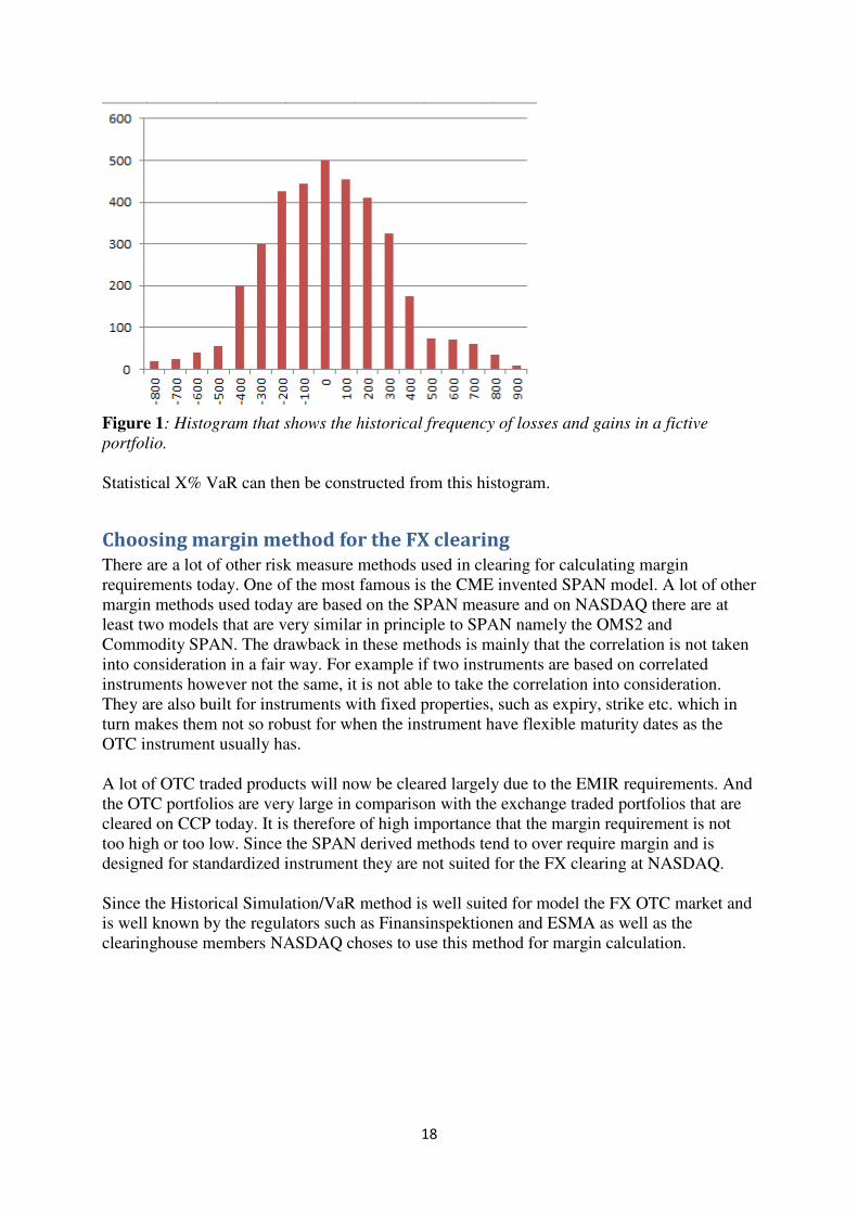
The most popular measure of risk in financial institutions in recent time is Value at Risk (VaR). VaR is a number that state a level that a loss will be higher than given a specified confidence level. VaR is composed of three parts. First you need to define a time period usually stated in number of days. The second part is the confidence level of the measure. The confidence level is typically between 95% and 99%. The third part is the loss amount that can be lost at the specified confidence interval in the specified time period. In the figure below the distribution represents the P/L of the portfolio. In the Loss tail of the distribution a quantile decides the VaR value of the portfolio.

There are mainly three methods for calculating VaR;

1. Historical methods 2. Variance/covariance (aka parametric) method and 3. Monte Carlo simulation

In all of the methods the main parts to estimate is the volatility of the portfolio and the correlation between the different instruments that is part of the portfolio. The calculation of the actual VaR measure is quite simple after the volatility and the correlation is estimated. The VaR measure is due to its predictability and that it is simple to understand very popular today by regulators and financial institutions. But it might not be the optimal measure for every market or all instruments. It is important to validate the VaR measure and also the method for calculating the VaR measure for different markets. In the variance/covariance method an assumption of distribution is made. The assumption is often that the distribution is Normal or Log-Normal. These assumptions have been shown in many papers to miss out on the leptokurtic nature of the real distributions. Next is the correlations estimated and quantified in a correlation matrix. If it is difficult to determine the distribution of the return series, historical simulation is a better approach. The leptokurtic nature is estimated as being the same in the future as it has been in the past.

17

A big challenge when using historical simulation is that all the historical prices need to be kept in good quality. Hence if changes occur in history that is forming the data to be non-representative there need to be measures to adapt the historical prices to fit into the time series. One example for the FX market is the creation of euro where a lot of different currencies disappeared and a new entered the market at one point in time.

Historical Simulation

A historical simulation base itself on the assumption that relative movements of financial instruments are a “perfect” predictor of future movements of these financial instruments. The difference between more model based VaR methodologies is that these relative movements are the whole distribution and not used to approximate the distribution. For a normal distribution one would use the historical data to calculate mean and standard deviation. This would perfectly describe the normal distribution which then could be used to calculate VaR measures. If 101 daily equity prices were used in a historical simulation (one day movements) one would get 100 changes that would be used in the simulation. Do notice that no other possible movements are allowed for the development of the price. We define the following

��(.) Price of the underlying i at time t

∆��(., D) The percentage difference between the price at time t and time t-k for underlying i. If k is omitted it is assumed that k=1

∆��(., D) = ��(.) − ��(. − D)��(. − D)

∆��(.) = ��(.) − ��(. − 1)��(. − 1)

�(., �E, … , �&) Price of instrument i at time t, as a function of all the underlying in the historical simulation.

�,G,H(.) Price of instrument i at time t, were each underlying has the market price at t but has moved the same way as it did between j and j-k. If k is omitted it is assumed that the movement is 1 day.

�,G,H(.) = �(., �E(.)(1 + ∆�E(J, D)),… , �&(.)(1 + ∆�&(J, D))) �,G(.) = �(., �E(.)(1 + ∆�E(J)),… , �&(.)(1 + ∆�&(J)))

The corresponding market value for a portfolio of instruments can be calculated for each scenario in the historical database. From these market values a histogram can be constructed.

18

Figure 1: Histogram that shows the historical frequency of losses and gains in a fictive

portfolio.

Statistical X% VaR can then be constructed from this histogram.

Choosing margin method for the FX clearing

There are a lot of other risk measure methods used in clearing for calculating margin requirements today. One of the most famous is the CME invented SPAN model. A lot of other margin methods used today are based on the SPAN measure and on NASDAQ there are at least two models that are very similar in principle to SPAN namely the OMS2 and Commodity SPAN. The drawback in these methods is mainly that the correlation is not taken into consideration in a fair way. For example if two instruments are based on correlated instruments however not the same, it is not able to take the correlation into consideration. They are also built for instruments with fixed properties, such as expiry, strike etc. which in turn makes them not so robust for when the instrument have flexible maturity dates as the OTC instrument usually has. A lot of OTC traded products will now be cleared largely due to the EMIR requirements. And the OTC portfolios are very large in comparison with the exchange traded portfolios that are cleared on CCP today. It is therefore of high importance that the margin requirement is not too high or too low. Since the SPAN derived methods tend to over require margin and is designed for standardized instrument they are not suited for the FX clearing at NASDAQ. Since the Historical Simulation/VaR method is well suited for model the FX OTC market and is well known by the regulators such as Finansinspektionen and ESMA as well as the clearinghouse members NASDAQ choses to use this method for margin calculation.

19

Risk factor set-up for NDF

The risk factors that are used for calculating risks are

• Discount function in both currencies

• The spot price From these the corresponding market value of the portfolio can be calculated according to the previously defined equation.

20

Numerical test

Historical data

The historical data that are available is the deposits that show the different rates for different G10 currencies. For each currency the deposits rate comes with different length. We also have the FX spot rates (fixing each day) available. Both the FX spot rate and the deposit data are from around 1980 until 2015. We also have data on historical NDF prices. But since the market is quite illiquid the data set is of quite bad quality. There can be holes in the data set for example. In the case there are holes the prices are simulated in the time period where the hole is. This makes the data set somewhat not fully reliable. The historical data on rates and spot FX rates, �K, Deposits for G10 currencies, L and NDF prices for non-G10 currencies are used to construct the discount factors from the historical rates in accordance with description in [ref 20].

L = �K3(*4M)+ These are used as inputs in calculating the market value that is used in the historical simulation. If we for example look at the 30 days discount function for GBP we can see that we have a

distinct period before the 2008/2009 period but after that it does not look the same at all. This

indicates that the 2008/2009 crisis changed the way historical simulation can predict future

changes in the FX market.

Figure 2. Discount function for 30 days GBP from 1993 to 2015.

0,992

0,993

0,994

0,995

0,996

0,997

0,998

0,999

1

1993-01-011995-09-281998-06-242001-03-202003-12-152006-09-102009-06-062012-03-022014-11-27

Dis

cou

nt

fact

or

Date

Discount function 30d GBP

21

Figure 3. Discount function for 30 days GBP from 2008 to 2010.

Figure 4. The graph shows the spot FX rate between GBP and USD (how many USD you

need to pay for one GBP).

If looking at the spot exchange rate between IDR and USD we can see that the shape of the

curve is comparable but not equal to the NDF prices for the same instruments.

0,992

0,993

0,994

0,995

0,996

0,997

0,998

0,999

1

2008-07-01 2008-10-09 2009-01-17 2009-04-27 2009-08-05 2009-11-13

Dis

cou

nt

fact

or

Date

Discount function 30d GBP

0

0,5

1

1,5

2

2,5

1980-04-01 1985-09-22 1991-03-15 1996-09-04 2002-02-25 2007-08-18 2013-02-07 2018-07-31

GBP USD FX Spot

22

Figure 4. Spot exchange rate between IDR and USD from 1982 to 2015.

Figure 5. NDF 3 month prices between USD and IDR from 1982 to 2015.

0

2000

4000

6000

8000

10000

12000

14000

1982-01-01 1987-06-24 1992-12-14 1998-06-06 2003-11-27 2009-05-19 2014-11-09 2020-05-01

0

2000

4000

6000

8000

10000

12000

14000

16000

1982-01-01 1987-06-24 1992-12-14 1998-06-06 2003-11-27 2009-05-19 2014-11-09 2020-05-01

23

Back-test the 99,2% 1-day VaR

We choose to do a validation test of the model by choosing a simple portfolio of 1 000 000 GBPUSD NDF (also called CSF since it is the G10 currencies). The agreed NDF rate is 1.3. The choice is made due to (i) we have good quality data in both USD and GBP which makes it more reliable and (ii) a one-directional, non-hedged portfolio is the most common portfolio. The back testing is performed such that we do a HS for 2500 days back to calculate the VaR for the next day. This is repeated for approximately 3500 days.

Figure 6. The red line represent the 99,2 1-day VaR calculated requirement based on

historical simulation of 2500 days back. The blue line represents the daily changes in

portfolio value of a portfolio consisting of one NDF for GBP to USD on a 30 year period.

There are 3198 test days performed.

Testing the null hypothesis that the VaR model is accurate

We assume that the daily returns of P&L is generated by an i.i.d Bernoulli process. An

indicator function is defined that take the value 1 if the loss is greater than the VaR one day

and 0 otherwise.

�N,+OE = P1, QR�+OE < −-U�E,N,+0V.ℎ39XQY3

Where �+OE is the ‘realized’ daily return or P&L on the portfolio from time t. Let �&,N denote

the number of successes. As is shown in [20] �&,N has a binomial distribution with >(�&,N) =

-60000

-40000

-20000

0

20000

40000

60000

2002-03-092003-07-222004-12-032006-04-172007-08-302009-01-112010-05-262011-10-082013-02-192014-07-04

De

lta

Date

24

Z[ and -(�&,N) = Z[(1 − [). The standard error of the estimate \Z[(1 − [) shows the

uncertainty around the expected value. We construct a confidence interval around the

expected value where we expect the number of exceedances is likely to fall. Since n is large

we assume that the distribution of �&,N is approximately normal. A two sided 95% confidence

interval for �&,N under the null hypothesis that the VaR model is accurate is approximately

(Z[ − 1.96\Z[(1 − [), Z[ + 1.96\Z[(1 − [)) In the test that was performed Z = 3198 and [ = 0.8% the standard error is

√25.6 ∗ 0.992 = 5.038 which gives a confidence interval of (16,35). The observed value of

exceedances in this case is 46. This means that we are rejecting the null hypothesis in this

case. It is hence obvious that we need to modify the HS in some way to better forecast the

behavior of the time series. There are a number of alternatives to the plain HS approach that is

validated here.

Looking at the graph it indicates that the section around 2008/2009 changes the VaR values

significantly. The figure also indicates that the model requires too much margin during the

period after 2008/2009. This is due to that the large volatility in the market during the

2008/2009 period is part of the historical simulation. The model is not adaptive to the changes

in the volatility.

Conclusion The simple back-testing of the HS/VaR model used indicates that the model have weaknesses that needs to be handled. The method does not model radical movements in the market very well. If looking at the events around 2008/2009 we see that the method reacts slowly and not considering the rapid change in the market and then it does not regress back after the large changes has impacted the value. Hence underestimating the risk within the volatile period and overestimating the risk long time afterwards when the volatility is low. This is a consequence of the known drawback of HS approach that for example is mentioned in [ref 22]. (i) “Extreme quantiles are notoriously difficult to estimate”, (ii) “quantile estimates obtained by HS tend to be very volatile whenever a large observation enters the sample” and (iii) “the method is unable to distinguish between periods of high and low volatility”. One change of the model that could be possible is to add a scaling factor that scales down the importance of prices that are further back in time. One standardized method of doing that is described in [ref 18, 25]. In this method exponential declining function is applied to the historical scenarios. With a decay rate, a, the function is defined for scenario Q in a set of Z historical scenarios according to:

a�4E(1 − a)1 − a&

Using this technique to create a new set of VaR where the decay rate is set to 0.99 we get the

green line in the graph. It can clearly be seen that it reacts much faster to changes. Hence a

25

simple change like that would have a great effect on how the HS model works for the variance

of the volatility.

Figure 7. The red line represent the 99,2 1-day VaR calculated requirement based on

historical simulation of 2500 days back. The green line represent the 1-day 99,2 VaR based

on historical simulation of 2500 days back with decay factor 0.99. The blue line represents

the daily changes in portfolio value of a portfolio consisting of one NDF for GBP to USD on

a 30 year period. There are 3198 test days performed.

To back test this approach we use Z = 3100 and [ = 0.8% to create a confidence interval for

the number of exceedances. The standard error becomes √24.8 ∗ 0.992 = 4.96 which then

renders the confidence interval (15,35). The observed number of exceedances in this case is

30 and hence we accept the null hypothesis in this case. Adding a decay rate factor to the HS

would hence be a small change in the model that would significantly improve the VaR

measure.

It would be of great interest to investigate the use of a model that in a more precise way

characterize the volatility clustering nature in the time series. The General Autoregressive

Conditional Heteroscedasticity (GARCH) model (proposed by Bollerslev 1986 based on

work done by Engel 1982) have been evaluated in many papers to be a good model for

catching the volatility clustering effect in financial time series. An extension to GARCH that

take into account the non-symmetric behavior of a financial time series was proposed by

Nelson 1991 and is called Exponential GARCH (EGARCH). EGARCH have shown to

provide a very good extension for financial time series.

An alternative is then to instead of using a non-parametric model like HS for estimating the

P/L distribution a fully parametric model where we make an assumption of conditional

normality for the P/L. The assumption on conditional normality is however an assumption

-60000

-40000

-20000

0

20000

40000

60000

2002-03-092003-07-222004-12-032006-04-172007-08-302009-01-112010-05-262011-10-082013-02-192014-07-04

De

lta

Date

26

that have been shown to not hold for real data. In [ref 23] Danielsson and de Vries show that

the conditional normality assumption is not well suited and an alternative to use Extreme

Value Theory (EVT) for estimating the return distribution of financial time series is explored.

A third complex alternative is explored in [ref 22] where McNeil and Frey explores a

combination of GARCH and EVT methods for representing the return distribution. They

represent the daily observed negative log return as �+ = b+ + c+ ∙ �+ where the innovation, �+ is a strict white noise. From this a one-step prediction of the quantile of the marginal

distribution as de+ = b+OE + c+OE ∙ fe is derived. fe is the upper qth quantile of the marginal

distribution of �+ which does not depend on t. The conditional variance c+g of the mean-

adjusted series h+ = �+ − b+ is estimated by using a AR(1)-GARCH(1,1) model where

c+g = [K + [E ∙ i+4Eg + j ∙ c+4Eg and the conditional mean b+ = a ∙ k+4E is fitted using a

pseudo-maximum-likelihood estimation with normal innovation to obtain estimation of the

parameters (al, [Kl , [El , j′). These are then used to calculate estimates of the conditional mean

and variance for day t+1;

b+OEl = a′ ∙ d+ c+OEg ′ = [K′ + [E′ ∙ i+g′ + j′ ∙ c+g′ Next McNeil and Frey estimate fe using extreme value theory and model the innovation as a

generalized pareto distribution to take the leptokurtic (fat-tail) distribution into account. The

model is back tested and it is shown that this model performs very well.

A view of the responsiveness of a GARCH(1,1) approach for the portfolio investigated in this

report can be seen in the Figure below where the 99% VaR is calculated using a GARCH(1,1)

approach is outlined (red line). In this figure it can be seen that it is a good hypothesis that this

approach would have handled the 2008/2009 crisis much more correct than the plain HS

approach that is chosen today.

27

Figure 8. The red line is a 99% VaR calculated with GARCH(1,1) approximation.

Recommendation for further analysis

The HS approach should be complemented with a decay factor for calculating the VaR

measure and a broader analysis of this adjustment should be done. It is though important to

note that the margin calculation with historical simulation is one of the mechanisms used for

managing risk within a clearinghouse. This is complemented with hypothetical scenarios as

well with the aim of catching events like the 2008/2009 crisis. Another future

recommendation is also to investigate if the approach proposed in [ref 22] would solve the

need for estimating the volatility in a more precise way for the FX market. Furthermore

should an investigation create more complex portfolios and validate if a GARCH estimation

of the volatility would give better VaR measure.

28

References

[1] Amini, Hamed and Filipović, Damir and Minca, Andreea. (2014) Systemic Risk with

Central Counterparty Clearing. Swiss Finance Institute Research Paper No. 13-34. Available

at SSRN: http://ssrn.com/abstract=2275376 or http://dx.doi.org/10.2139/ssrn.2275376

[2] Tucker, Paul (2011) Clearing houses as system risk managers. At the DTCC-CSFI Post

Trade Fellowship Launch, London 1 June 2011

[3] Artzner, P., Delbaen, F., Eber, J., Heath, D., (1999). Coherent measures of risk.

Mathematical Finance 93., 203–228.

[4] Gai, P. and Kapadia, S. (2010). Contagion in Financial Networks. Proceedings of the

Royal Society A, 466(2120):2401-2423.

[5] Glasserman, P. and Young, H. P. (2013). How likely is contagion in financial networks? Journal of Banking and Finance, to appear. [6] Minca, A. and Sulem, A. (2014). Optimal control of interbank contagion under complete information. Statistics & Risk Modeling, 31(1):23-48.

[7] Stulz, R. M. (2010). Credit Default Swaps and the Credit Crisis. Journal of Economic

Perspectives, 24(1):73-92.

[8] Amini, H., Cont, R., and Minca, A. (2013). Resilience to contagion in financial networks.

Mathematical Finance.

[9] Acemoglu, D., Ozdaglar, A., and Tahbaz-Salehi, A. (2015). Systemic risk and stability in

financial networks. American Economic Review, 105(2): 564-608

[10] Chinazzi, Matteo and Fagiolo, Giorgio (2013). Systemic Risk, Contagion, and Financial

Networks: A Survey. Available at SSRN: http://ssrn.com/abstract=2243504 or

http://dx.doi.org/10.2139/ssrn.2243504

[11] http://www.lchclearnet.com/risk-collateral-management/margin-methodology/pairs

[12] NASDAQ Historical Simulation – Methodology guide for margining FX products.

http://www.nasdaqomx.com/europeanclearing/risk-management

[13] Arnsdorf, M. (2012). Central counterparty risk. arXiv preprint arXiv:1205.1533.

[14] http://www.riksdagen.se/sv/Dokument-Lagar/Lagar/Svenskforfattningssamling/Lag-

2013287-med-komplettera_sfs-2013-287/?bet=2013:287

[15] http://www.fi.se/Regler/Derivathandel-Emir/

[16] http://www.esma.europa.eu/page/post-trading

[17]http://ec.europa.eu/finance/financial-markets/derivatives/index_en.htm

29

[18] Hull, John C (2012). Risk Management and Financial Institutions, Third Edition (Wiley

Finance). ISBN: 978-1-118-95594-9

[19]http://www.esma.europa.eu/system/files/public_register_for_the_clearing_obligation_und

er_emir.pdf

[20] Lang, Harald (2012). Lectures on Financial Mathematics.

https://people.kth.se/~lang/finansmatte/fin_note_dist.pdf

[21] Alexander, Carol (2014). Market Risk Analysis: Volume IV; Value-at-risk models.

ISBN: 9780470997888

[22] Alexander J McNeil, Rudiger Frey (2000). Estimation of Tail-Related Risk Measures for

Heteroscedastic Financial Time Series: an Extreme Value Approach. Journal of Empirical

Finance 7 2000 271–300

[23] Danielsson, J., de Vries, C., (1997). Tail index and quantile estimation with very high

frequency data. Journal of Empirical Finance 4, 241–257.

[24] Barone-Adesi, G., Bourgoin, F., Giannopoulos, K. (1998). “Don’t look back”. Risk 11

(8).

[25] Richardson, Matthew P. and Boudoukh, Jacob and Whitelaw, Robert (1997). The Best of

Both Worlds: A Hybrid Approach to Calculating Value at Risk. Available at SSRN:

http://ssrn.com/abstract=51420 or http://dx.doi.org/10.2139/ssrn.51420

[26] Bollerslev, T. (1986). Generalized autoregressive conditional heteroskedasticity. Journal

of Econometrics, 31:307–327, 1986

[27] Bollerslev, T., Chou, R.Y., Kroner, K.F. (1992). ARCH modeling in finance: a review of

theory and empirical evidence. Journal of Econometrics 52:5 – 59

[28] Engle, R. F. (1982). Autoregressive Conditional Heteroskedasticity with estimates of the

variance of United Kingdom inflation. Econometrica, 50:987–1007

[29] Nelson, D. B. (1991). Conditional Heteroskedasticity in Asset Returns: A New Approach.

Econometrica, 59:347–370

30

Appendix 1 – GARCH (General Autoregressive Conditional

Heteroskedasticity)

Robert Fry Engle III defined a time series characterizing model called Autoregressive

Conditional Heteroskedasticity (ARCH) in 1982 [ref 28]. It is modeling the volatility

clustering effect that is very often present in financial time series. In an ARCH model the

error term i+ is defined by

i+ = c+ ∙ f+ Where c+ represents the time-dependent standard deviation and f+ represent the stochastic

white noise process. The c+ is modeled in

c+g = [K +n[� ∙ i+4�ge

�oE

Where the parameters [K > 0 and [� ≥ 0 for Q = 1,… , r. r represent “the order of the model”.

The ARCH(q) model is then fitted by the use of for example and least square method. The lag

length of the errors is then tested with a Lagrange multiplier test (in the process proposed by

Engle).

Tim Bollerslev proposed a generalization of the ARCH(q) model in 1986 by proposing to

“allow for past conditional variances in the current conditional variance equation” [ref 26].

This means in practice to model the time-dependent standard deviation by introducing a s

ordered term for modeling in the dependency on cg. The GARCH(p,q) model is defined as

c+g = [K +n[� ∙ i+4�ge

�oE+nj� ∙ c+4�g

t

�oE

Where j� ≥ 0 for Q = 1,… , s.

Since higher order of these models seldom outperforms lower order GARCH models a

common model to use is the simplest GARCH(1,1). see [ref 2] for one performance

evaluation of lower order GARCH models. A GARCH(1,1) model is defined by:

c+g = [K + [E ∙ i+4Eg + j ∙ c+4Eg

The GARCH model is fitted with maximum likelihood estimation.

There exist a number of extensions for the GARCH model that can be of usage for different

purposes. An often used variant of the GARCH model is the Exponential GARCH

(EGARCH). This is useful in financial series mostly because the asymmetric nature of the

positive and negative shocks that is often the case. The model was introduced by Nelson 1991

[ref 29].