Managing and Querying Derived Nutrient Parameters in the

Bachelor Thesis

Managing and Querying Derived NutrientParameters in the Swiss Feed Database

Hannes TreschSarnen, Switzerland

supervised byProf. Dr. M. Böhlen and F. Cafagna

Department of Informatics,University of Zurich

November 30, 2011

Abstract

The aim of the thesis has been to integrate the computation of derived nutrients into theSwiss animal feed database. Derived nutrients are parameters calculated by a formula thatinvolves other nutrient parameters. The computation of these parameters replaces expensivechemical lab analyses. In order to get a meaningful temporal distribution of derived nutrients,an efficient method that supports time-varying regressions must be found.

For that, different SQL-queries, SQL-views and PL/pg SQL functions are implemented andpresented in this document. The most efficient solution is then used for the implementationof an extension to the actual web application, so that all the functionalities that currentlyexist for non-derived nutrients are to be supported for derived nutrients as well.

I

II

Zusammenfassung

Das Ziel dieser Arbeit bestand darin, eine automatisierte Berechnung von abhängigenNährwerten in die schweizerische Futtermitteldatenbank zu integrieren. Diese sogenannten’abgeleiteten’ Nährwerte (engl. derived nutrients) werden nicht durch chemische Analysen er-mittelt, sondern sind abhängig von anderen Nährwerten und werden mittels Formeln berech-net. Um aussagekräftige Daten über die zeitliche Veränderung von abgeleiteten Nährwertenzu erhalten, musste eine Methode ausgearbeitet werden, die eine zeitbezogene Regressions-berechnung unterstützt.

Dazu werden in dieser Arbeit verschiedene Ansätze präsentiert, die mit Hilfe von SQL-queries, SQL-views und PL/pg SQL -functions umgesetzt wurden. Die effizienteste Implemen-tierung wurde dann in die aktuelle Web Applikation integriert, sodass alle Funktionalitätenauch für abhängige Nährstoffe unterstützt sind.

III

IV

Contents

1 Introduction to the Swiss Feed Database 1

2 Task definition and overview 3

3 Database schemas 5

3.1 Schema Version 1.0 . . . . . . . . . . . . . . . . . . . . . . . . . . . . . . . . . 53.2 Schema Version 2.0 . . . . . . . . . . . . . . . . . . . . . . . . . . . . . . . . . 7

4 Analyses and classification of derived nutrients 9

4.1 Classification of derived nutrients . . . . . . . . . . . . . . . . . . . . . . . . . 94.2 Analyses of nutrient abbreviations and formula expressions . . . . . . . . . . 10

5 Design of Views, Queries and Algorithms 11

5.1 Materialized views . . . . . . . . . . . . . . . . . . . . . . . . . . . . . . . . . 115.1.1 Introduction to views in SQL . . . . . . . . . . . . . . . . . . . . . . . 115.1.2 Views with up-to-date values . . . . . . . . . . . . . . . . . . . . . . . 11

5.2 Standard SQL Implementation . . . . . . . . . . . . . . . . . . . . . . . . . . 135.2.1 Queries for time-varying regressions . . . . . . . . . . . . . . . . . . . 135.2.2 Queries specified on database schema Version 2.0 . . . . . . . . . . . . 165.2.3 Explanation for performance problems . . . . . . . . . . . . . . . . . . 17

5.3 Window Functions . . . . . . . . . . . . . . . . . . . . . . . . . . . . . . . . . 195.4 Implementation of Algorithm in Java . . . . . . . . . . . . . . . . . . . . . . . 205.5 PL/pg SQL Functions . . . . . . . . . . . . . . . . . . . . . . . . . . . . . . . 24

5.5.1 Introduction to PL/pg SQL Functions . . . . . . . . . . . . . . . . . . 245.5.2 Implementation approach using a 3-dimensional-Array . . . . . . . . . 245.5.3 Implementation approach using a string array . . . . . . . . . . . . . . 275.5.4 Implementation approach using cursor variables . . . . . . . . . . . . . 285.5.5 Performance comparison of implementation approaches . . . . . . . . 31

6 Implementation of an extension to the Swiss Feed Database 33

6.1 Introduction to Swiss Feed Database web application Version 2.0 . . . . . . . 336.2 Overview of tasks for the integration of derived nutrients into the web application 366.3 Insertion of derived nutrients into the nutrient select field [Task 1] . . . . . . 38

6.3.1 Creation of table containing formulas . . . . . . . . . . . . . . . . . . 386.3.2 Query . . . . . . . . . . . . . . . . . . . . . . . . . . . . . . . . . . . . 396.3.3 PHP / JavaScript Implementation . . . . . . . . . . . . . . . . . . . . 40

6.4 Update select fields depending on selected derived nutrients [Task 2] . . . . . 416.4.1 Query . . . . . . . . . . . . . . . . . . . . . . . . . . . . . . . . . . . . 41

V

6.4.2 PHP / JavaScript Implementation . . . . . . . . . . . . . . . . . . . . 426.5 Compute time-varying regressions [Task 3] . . . . . . . . . . . . . . . . . . . . 43

6.5.1 PL/pg SQL Function for temporal results . . . . . . . . . . . . . . . . 436.5.2 PHP / JavaScript Implementation of temporal results . . . . . . . . . 44

6.6 Compute derived nutrient values grouped by measurement samples [Task 4] . 466.6.1 Query . . . . . . . . . . . . . . . . . . . . . . . . . . . . . . . . . . . . 466.6.2 PL/pg SQL Function for sample results . . . . . . . . . . . . . . . . . 476.6.3 PHP / JavaScript Implementation for sample results . . . . . . . . . . 48

7 Summary 49

VI

List of Figures

1.1 Web application, Version 1.0 . . . . . . . . . . . . . . . . . . . . . . . . . . . 21.2 Web application, Version 2.0 . . . . . . . . . . . . . . . . . . . . . . . . . . . 2

3.1 Simplified schema of the Swiss feed database, Version 1.0 . . . . . . . . . . . 53.2 Schema of the Swiss feed database, Version 2.0 . . . . . . . . . . . . . . . . . 7

6.1 Selection part of the web application . . . . . . . . . . . . . . . . . . . . . . . 336.2 Sample enlistment . . . . . . . . . . . . . . . . . . . . . . . . . . . . . . . . . 346.3 Map with marked measurement locations . . . . . . . . . . . . . . . . . . . . 346.4 Line-diagram and Scatter-diagram . . . . . . . . . . . . . . . . . . . . . . . . 356.5 Aggregation table with statistical information . . . . . . . . . . . . . . . . . . 356.6 Visualization of task 1 concerning the integration of derived nutrients . . . . 366.7 Visualization of task 2 concerning the integration of derived nutrients . . . . 366.8 Visualization of task 3 concerning the integration of derived nutrients . . . . 376.9 Visualization of task 4 concerning the integration of derived nutrients . . . . 37

VII

VIII

List of Tables

4.1 Sample derived nutrients with their formulas . . . . . . . . . . . . . . . . . . 94.2 Classification of nutrient abbreviations . . . . . . . . . . . . . . . . . . . . . . 104.3 Supported and not supported formula expressions . . . . . . . . . . . . . . . . 10

5.1 First combining pass considering the timestamps of table RP as fix . . . . . . 135.2 Second combining pass considering the timestamps of table ALA as fix . . . . 145.3 Calculated derived nutrient values for #RP_ALA . . . . . . . . . . . . . . . 145.4 Comparison of estimated execution costs . . . . . . . . . . . . . . . . . . . . . 185.5 Approach with window functions lag() and lead() . . . . . . . . . . . . . . 195.6 Combining process I: Timestamps of nutrient ZUCK are considered as fix . . 215.7 Combining process II: Timestamps of nutrient TSO are considered as fix . . . 225.8 Illustration of 3-dimensional-array allcomp[][][] . . . . . . . . . . . . . . . 245.9 Combining process in the 3-dimensional array . . . . . . . . . . . . . . . . . . 255.10 Illustration of string array allcomp[] . . . . . . . . . . . . . . . . . . . . . . . 275.11 Combining pass with two cursors (on the result set of ZUCK, resp. TSO) . . 285.12 Combining pass with two cursors (on the result set of ZUCK, resp. ETOH) . 285.13 Combing pass with ZUCK, TSO and ETOH using cursors . . . . . . . . . . . 305.14 Performance comparison of PL/pg SQL functions . . . . . . . . . . . . . . . . 31

6.1 Table t_formulas containing derived nutrients (id 10-13: fictive nutrients) . 386.2 Extract of table t_formula_feed and d_feed . . . . . . . . . . . . . . . . . 38

IX

X

Chapter 1

Introduction to the Swiss FeedDatabase

This thesis is part of the Swiss Feed Database project. The aim of the project is to producea public service for companies, private farmers, and research institutions to get informationabout several nutrient parameters of specific feed types. This information can be used foran optimal and quality-conscious choice of feeds for a specific animal type. The databasecontains currently information for 155 nutrients and over 600 animal feed types. These dataare collected through chemical analyses on feed sample measurements that are taken from allparts of Switzerland. All the information about the nutrients is stored in a database and cancurrently be accessed by a web application.1[1]

At the moment, the University of Zurich collaborates with Agroscope (Bundesamt fürLandwirtschaft) to design and implement new database techniques in order to improve theanalysis of the feed data. In particular, an analysis of time-varying feed data for a desiredperiod and specific biological or geographical parameters is required. Figure 1.1 shows theactual web application, Figure 1.2 is a new web application that is currently being developedat University of Zurich. In the new web application based on a new database design (Ver-sion 2.0),0 information about nutrients for specific geographical conditions and desired timeperiods can be retrieved and displayed in suitable form.

1The current web application can be accessed here: http://www.feed-alp.admin.ch/start.php

1

Figure 1.1: Web application, Version 1.0

Figure 1.2: Web application, Version 2.0

2

Chapter 2

Task definition and overview

The nutrient parameters of several different animal feeds are measured by chemical analyses.Apart from these measured data values, some nutrient parameters are computed by the helpof a formula. This formula is an algebraic expression that involves a various number ofnutrient components. The computation of such derived nutrients replaces expensive chemicallab analyses and results in approximate values.

Because it is hard to update all the derived nutrient values manually, a method thatcomputes derived nutrients automatically is needed. In addition to that, the history of de-rived nutrient values should be stored in an appropriate way, so that based on the temporaldistribution of these values, meaningful information can be extracted.

So, the aim of the thesis can be summarized as follows:

• Integrate the computation of derived nutrients into the Swiss feed database and

• implement an extension to the web application that supports time-varying regressions.

The thesis in hand is structured as follows: In a first step, the schemas that are used inthis project are presented with some sample queries to get familiar with the database. Afterthat, the derived nutrients are analyzed, classified and possible methods to compute themare presented.

Initially, it has been supposed to use views as a support to retrieve the values for de-rived nutrients. Because of performance problems, an alternative solution with a procedurallanguage will be proposed.

Finally, some PL/pg SQL functions are defined that compute the values of derived nutri-ents in a temporal way. With the help of these functions, an extension to the web application(Version 2.0) is implemented, so that all functionalities of the web application will be sup-ported for derived nutrients.

3

4

Chapter 3

Database schemas

3.1 Schema Version 1.0

The database schema of the Swiss feed database, Version 1.0, is shown in a simplified versionin Figure 3.1. The illustration contains just the most important relations to give an overviewon the database schema.

The most of the implementation approaches that are presented in chapter 5 are specified onthe second version of the database. Nevertheless, the schema of the first version is presentedhere, because it is used for the first approach described in chapter 5.1.

Figure 3.1: Simplified schema of the Swiss feed database, Version 1.0

5

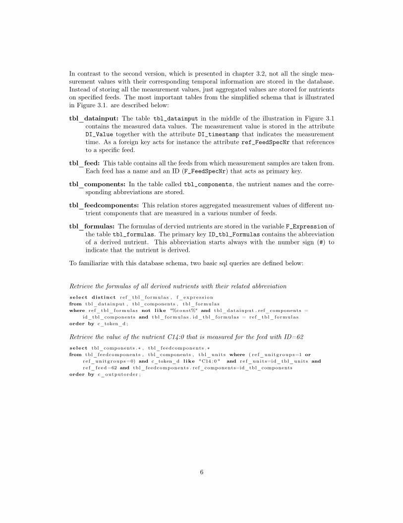
In contrast to the second version, which is presented in chapter 3.2, not all the single mea-surement values with their corresponding temporal information are stored in the database.Instead of storing all the measurement values, just aggregated values are stored for nutrientson specified feeds. The most important tables from the simplified schema that is illustratedin Figure 3.1. are described below:

tbl_datainput: The table tbl_datainput in the middle of the illustration in Figure 3.1contains the measured data values. The measurement value is stored in the attributeDI_Value together with the attribute DI_timestamp that indicates the measurementtime. As a foreign key acts for instance the attribute ref_FeedSpecNr that referencesto a specific feed.

tbl_feed: This table contains all the feeds from which measurement samples are taken from.Each feed has a name and an ID (F_FeedSpecNr) that acts as primary key.

tbl_components: In the table called tbl_components, the nutrient names and the corre-sponding abbreviations are stored.

tbl_feedcomponents: This relation stores aggregated measurement values of different nu-trient components that are measured in a various number of feeds.

tbl_formulas: The formulas of dervied nutrients are stored in the variable F_Expression ofthe table tbl_formulas. The primary key ID_tbl_Formulas contains the abbreviationof a derived nutrient. This abbreviation starts always with the number sign (#) toindicate that the nutrient is derived.

To familiarize with this database schema, two basic sql queries are defined below:

Retrieve the formulas of all derived nutrients with their related abbreviationselect dist inct ref_tbl_formulas , f_expres s ionfrom tbl_datainput , tbl_components , tbl_formulaswhere re f_tbl_formulas not l ike "%const%" and tbl_datainput . ref_components =

id_tbl_components and tbl_formulas . id_tbl_formulas = ref_tbl_formulasorder by c_token_d ;

Retrieve the value of the nutrient C14:0 that is measured for the feed with ID=62select tbl_components .∗ , tbl_feedcomponents .∗from tbl_feedcomponents , tbl_components , tb l_uni t s where ( re f_unitgroups=1 or

re f_unitgroups=0) and c_token_d l ike "C14 : 0 " and r e f_un i t s=id_tbl_units and

re f_feed=62 and tbl_feedcomponents . ref_components=id_tbl_componentsorder by c_outputorder ;

6

3.2 Schema Version 2.0

Figure 3.2 depicts the schema of the Swiss Feed Database (Version 2.0). The table that iscalled fact_table is the center of the schema. It contains all the information of a mea-surement that is taken from a specific sample. The measure_pk is the primary key of thistable. Apart from the measurement value (quantity) and the sample identification number(lims_number) there are some other fields that act as foreign keys refering to other relations.

Figure 3.2: Schema of the Swiss feed database, Version 2.0

Because of the special representation of the table named time, this relation has to bementioned in detail: As illustrated in Figure 3.2 , it can be stated four different time detailsin relation to a certain measurement. These are the Harvest Date, the Sample Date, theArrival Date and the Analysis Date. This means, a measurement can be related to morethan just one timestamp. The table time has an attribute named moment that identifies whatkind of date the time_key is representing. So, the table fact_table can contain up to fourtuples for the same measurement value, but with a different time_key. This ensures that allthe different details according the measurement time are stored in an efficient way.

7

8

Chapter 4

Analyses and classification ofderived nutrients

4.1 Classification of derived nutrients

The values of derived nutrient parameters are computed with algebraic expressions whichinvolve a various number of nutrient parameters. These nutrient parameters can be

• values that are measured by chemical analyses, or

• derived nutrients that are calculated based on other derived nutrient parameters.

The latter implies that such regression can also be recursive. Table 4.1 shows some sampleformulas of derived nutrients. The abbreviations of the nutrients in Table 4.1 are those ofthe first database version. The derived nutrients in row 2, 4 and 5 correspond to a formulathat is recursive, whereas the derived components are in bold. In the square brackets afterthe abbreviations, the measuring unit is defined, followed by the drying reference.1

ref_tbl_formulas f_expression

#Biotin[åµg_kg FS] TS[g_kg] * Biotin[åµg_kg TS] / 1000

#BE_Maisganzpfl[MJ_kg TS] 0.0196 * OS[g_kg TS]

#OS[g_kg TS] 1000 - RA[g_kg TS]

#C20:4n-6[g_kg FS] TS[g_kg] * C20:4n-6[g_kg TS] / 1000

#MPP_NEL[kg Milch_kg TS] NEL[MJ_kg TS] / 3.14

#NEL[MJ_kg TS] 0.9752 * (0.463 + 0.24 * q) * UE[MJ_kg TS]

Table 4.1: Sample derived nutrients with their formulas

The principle of recursive formulas is illustrated by the simple formula of the nutrientnamed #BE_Maisganzpfl[MJ_kg TS] that is listed in the second row of the table above.

Start formula: 0.0196 * OS[g_kg TS]↓

Expanded formula: 0.0196 * (1000 - RA[g_kg TS])

1TS = Trockenfutter, FS = Frischfutter

9

4.2 Analyses of nutrient abbreviations and formula ex-

pressions

The computation approaches that are presented in the chapters 5.4 and 5.5 are based onthe principle of a formula evaluator. This means, that all the abbreviations that occur ina formula are extracted from this formula. For each abbreviation is then a correspondingmeasurement value assigned, such that the computation can be performed and a derivednutrient value results.

To extract all the involved abbreviations from the formula correctly, the structure of theabbreviations has to be analyzed to define in what way the formulas have to be written. Forthat, all the nutrient abbreviations of database schema 2.0 were analyzed and grouped in anappropriate way. In Table 4.2, these groups are listed with a corresponding example.

group description abbreviation_de name_deGroup 1 just letters [A-Z] GLY GlycinGroup 2 [0-9] and [A-Z] C3OH MilchsäureGroup 3 ’_’-symbol is involved K_VA Retinol (Vitamin A)Group 4 ’-’ -symbol is involved CU-PF Kupfer Pet-food

Table 4.2: Classification of nutrient abbreviations

In most cases, the abbreviation names are only composed of letters and numbers. In somecases the hyphen- or the underscore-symbol is involved (group 3, resp. group 4). Speciallyif the abbreviation contains a hyphen-symobl, special consideration is required such that thehyphen is not recognized as a minus operator. For that, it is important to put a blank(�) before or after each minus-operator that is involved in a formula. For all the othermathematical operators, it doesn’t depend whether there is a blank between the operatorand the abbreviation. The list below illustrates this rule and shows the kind of formulas thatare supported by the PL/pg functions that are presented later in chapter 5.5.

1. K_VA^2�+�(CU-PF�-�C10)�*�C3OH�+�GLY�/�22. K_VA^2+(CU-PF-C10)*C3OH+GLY/23. K_VA^2+(CU-PF�-C10)*C3OH+GLY/2

Table 4.3: Supported and not supported formula expressions

The second expression in this list is not valid, because the expression CU-PF-C10 isconsidered one nutrient. To split up the expression correctly in those base components, theremust be an associated blank for each minus-operator. This is the case in example formulanumber 1 and and also in example formula number 3. However, the second formula is notsupported by the algorithm approaches that are described in the chapters 5.5.

For all the formulas of derived nutrients, the most common mathematical operators as ’+’,’-’, ’*’, ’/’ and ’^’ are used. All these are supported by postgreSQL whereby the computationof derived nutrients within pg SQL should be possible without any restrictions.[5]

10

Chapter 5

Design of Views, Queries andAlgorithms

5.1 Materialized views

5.1.1 Introduction to views in SQL

In a first approach, it was supposed to use views for the computation of the derived nutrients.According to SQL terminology, a view can be defined as a virtual table that is derived fromother tables. So, a view defines a function from a set of base stored tables to a derived table.Every time a view is referenced, this function is called and the virtual table is filled withtuples. A view can also be called a virtual table, because the tuples that are representinga view are not stored on a single table in the database. In contrast to that, in base storedtables, all the tuples of a relation are stored in the database.[3][4]

5.1.2 Views with up-to-date values

In a first phase, database schema Version 1.0 was used to create for each derived nutrient aview that is representing the up-to-date values for each feed type. So, it resulted in total 364view definitions of different complexity. The query to create such a view is illustrated on thenext page by the example of a basic formula.

The basic idea to get the up-to-date value of a derived nutrient is to use for the calculationthe newest available data for each involved component of a given formula. The views arespecified on the database schema version 1.0 and are composed of the following attributes:

1. The first attriubte is the ID of the feed type (f_feedspecnr).

2. The second attribute is the derived nutrient value (value) that is calculated in the viewdefintion as it is explained on the next page.

3. Additionally, the date that refers to a the specific derived nutrient value is specified inthe third attribute (timestamp).

The listing on the next page shows a simple example how such a SQL view of a derivednutrient is created.

11

As an example, the derived nutrient with the abbreviation #BE_Raufutter is used:

Create a view that computes the up-to-date value of a derived nutrient

Derived nutrient: #BE_Raufutter[MJ_kg TS]Formula: 0.0188 * OS[g_kg TS] + 0.0078 * RP[g_kg TS]View attributes: f_feedspecnr value timestampDatabase schema: Version 1.0

1 create view BE_Raufutter$MJ_kg$TS as

2 select f_feedspecnr ,3 (0 .0188 ∗4 ( select cast (value as numeric )5 from OS$g_kg$TS6 where OS$g_kg$TS . f_feedspecnr=tbl_feed . f_feedspecnr and value i s not null )78 + 0.0078 ∗9

10 ( select cast (value as numeric )11 from parameters , tbl_components , tbl_datainput12 where r e f_feedspecnr=id_feed and id_feed=f_feedspecnr and ref_components=

id_tbl_components13 and id_param=id_tbl_components and c_token_d=’RP ’ order by tstamp desc limit

1)14 )1516 as value ,1718 ( select max( time_stamp )19 from

20 ( ( select tstamp as time_stamp21 from parameters , tbl_components , tbl_datainput22 where id_param=id_tbl_components and id_feed=f_feedspecnr and f_feedspecnr=

re f_feedspecnr and id_tbl_components=ref_components and ( c_token_d=’RP ’ ) and value i s not null and re f_tbl_formulas=’#constant ’ )

2324 union a l l

2526 ( select timestamp as time_stamp27 from OS$g_kg$TS28 where tb l_feed . f_feedspecnr=OS$g_kg$TS . f_feedspecnr ) ) as max_view29 ) as timestamp

3031 from tb l_feed order by f_feedspecnr ;

As already mentioned, the calculation of the formula is performed with the newest avail-able measurement values for each nutrient component. The formula that corresponds to theconsidered derived nutrient is composed of two numerical and two nutrient components. Thenutrients that are involved are RP[g_kg TS] (Rohprotein) and OS[g_kg TS] (OrganischeSubstanz):

• The newest available value for the second nutrient component named RP[g_kg TS]

is retrieved in the subquery defined from line 10 to 13. This is done with the helpof the LIMIT-clause. The join in the WHERE-clause (id_feed=f_feedspecnr) of thesubquery guarantees, that for each feed just the corresponding data is used for thecomputation of a derived value.

• The other nutrient component that occurs in the formula is OS[g_kg TS] and can beidentified as a derived component. This means that those values are stored in a view.The subquery from line 4 to 6 shows how the value for a specific feed is retrieved froma defined view.

12

In the select statement of the view definition above, the computation of the derived nutrientnamed #BE_Raufutter[MJ_kg TS] is done. For that, the selected values for RP and OSare used. This means that the formula (0.0188 * OS[g_kg TS] + 0.0078 * RP[g_kg TS]) iscomputed with the selected OS- resp. RP-value.

Finally, for each feed type, the ID of the feed (f_feedspecnr), the computed derivedvalue and an associated timestamp is filled into the virtual table. The third attribute of theview named timestamp, represents the date of the derived nutrient value. This timestampis the newest one of all the nutrient components of the formula. That can be done by amax-aggregation over all the involved components (line 18).

5.2 Standard SQL Implementation

5.2.1 Queries for time-varying regressions

The views that are presented in the previous chapter contain just the up-to-date values of anutrient per each feed. In a next step, the views had to be adjusted, so that the history ofa specific derived nutrient can be stored. An approach how time-varying regressions can becomputed in a appropriate way is given in this sub-chapter.

The basic idea to get information of how the values of derived nutrients change overtime is the following: For the calculation of a derived nutrient parameter at a specific time,we take measurement values of all involved components that have the same timestamp orare even from the same measurement sample. But in order to get a meaningful historicalrepresentation, we need more data values than just those that come from the same sample.

A possible solution to this problem is to take for all involved components the measurementvalues that are the closest to each other according to their timestamp.

The basic idea of this approach is explained by the following example: Assume that wehave a derived nutrient with the abbreviation #RP_ALA that is calculated by the formula(RP * ALA) / 10. In this case, we create for RP and ALA a table that contains all themeasurement values of the associated nutrient. The computing process of this example canbe structured in two parts, whereas in each part the timestamps of a different component arein focus. These two parts are presented below:

1. Table 5.1 shows the first part, where the timestamps of RP are considered as fix. Foreach row in table RP, we search for a value in the other component where the timestampis the closest to that of the RP value.

Table 5.1: First combining pass considering the timestamps of table RP as fix

The first result value in Table 5.1 would be calculated by the expression (3.1*10)/10.The ALA-value from the second row is taken for the calculation, because the related

13

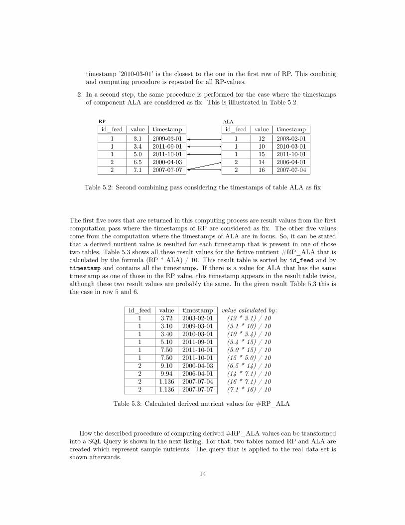
timestamp ’2010-03-01’ is the closest to the one in the first row of RP. This combinigand computing procedure is repeated for all RP-values.

2. In a second step, the same procedure is performed for the case where the timestampsof component ALA are considered as fix. This is illlustrated in Table 5.2.

Table 5.2: Second combining pass considering the timestamps of table ALA as fix

The first five rows that are returned in this computing process are result values from the firstcomputation pass where the timestamps of RP are considered as fix. The other five valuescome from the computation where the timestamps of ALA are in focus. So, it can be statedthat a derived nurtient value is resulted for each timestamp that is present in one of thosetwo tables. Table 5.3 shows all these result values for the fictive nutrient #RP_ALA that iscalculated by the formula (RP * ALA) / 10. This result table is sorted by id_feed and bytimestamp and contains all the timestamps. If there is a value for ALA that has the sametimestamp as one of those in the RP value, this timestamp appears in the result table twice,although these two result values are probably the same. In the given result Table 5.3 this isthe case in row 5 and 6.

id_feed value timestamp value calculated by :1 3.72 2003-02-01 (12 * 3.1) / 101 3.10 2009-03-01 (3.1 * 10) / 101 3.40 2010-03-01 (10 * 3.4) / 101 5.10 2011-09-01 (3.4 * 15) / 101 7.50 2011-10-01 (5.0 * 15) / 101 7.50 2011-10-01 (15 * 5.0) / 102 9.10 2000-04-03 (6.5 * 14) / 102 9.94 2006-04-01 (14 * 7.1) / 102 1.136 2007-07-04 (16 * 7.1) / 102 1.136 2007-07-07 (7.1 * 16) / 10

Table 5.3: Calculated derived nutrient values for #RP_ALA

How the described procedure of computing derived #RP_ALA-values can be transformedinto a SQL Query is shown in the next listing. For that, two tables named RP and ALA arecreated which represent sample nutrients. The query that is applied to the real data set isshown afterwards.

14

Compute for each feed time-varying values of a derived nutrient

Derived Nutrient: #RP_ALAFormula: (RP * ALA ) / 10Result attributes: id_feed value timestamp

1 (2 ( select RP. id_feed , (RP. value ∗ ALA. value ) / 10 as value , RP. tstamp as timestamp

3 from RP, ALA4 where RP. id_feed=ALA. id_feed and

5 ALA. tstamp6 IN (7 ( select ALA2. tstamp8 from ALA as ALA29 where RP. id_feed=ALA2. id_feed

10 order by abs ( cast (ALA2. tstamp as date ) − cast (RP. tstamp as date ) )11 l imit 1)12 )13 order by RP. id_feed )14 union

1516 ( select ALA. id_feed as f , ALA. value ∗ RP. value as v , ALA. tstamp as t17 from RP, ALA18 where RP. id_feed=ALA. id_feed and

19 RP. tstamp20 IN (21 ( select RP2. tstamp22 from RP as RP223 where RP2. id_feed=ALA. id_feed24 order by abs ( cast (ALA. tstamp as date ) − cast (RP2 . tstamp as date ) )25 l imit 1)26 )27 )28 order by id_feed , timestamp

29 ) ;

The query above that retrieves time-varying values for a derived nutrient called #RP_ALAis described below:

1. From line 2 to 15, the first computation pass is done, where the timestamps of RP areconsidered as fix. This is previously visualized in the Table 5.1.

(a) It retrieves the id_feed, the calculated value, and the timestamp of the RPmeasurement that is used for the computation.

(b) In the subquery of the IN-clause (line 7 to 11), the timestamp of an ALA-measurementis retrieved that is the closest to the one of the considered RP-measurement. Thisis done by subtracting the timestamp values of the components that are consid-ered. This guarantees that the ALA measurement is used, whose timestamp isthe closest to that of the considered RP-measurement. Instead of doing the sub-traction of timestamps, the postgres date-function age(timestamp, timestamp)could also be used to compare timestamps. [5]

2. From line 16 to 28, the second computation pass is done, where the timestamps of ALAare considered as fix. This is visualized in the Table 5.2 and works in the same way aspreviously described by the example of RP.

15

5.2.2 Queries specified on database schema Version 2.0

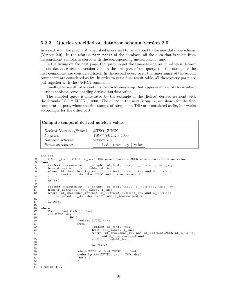
In a next step, the previously described query had to be adapted to the new database schema(Version 2.0). In the relation fact_table of the database, all the data that is taken frommeasurement samples is stored with the corresponding measurement time.

In the listing on the next page, the query to get the time-varying result values is definedon the database schema version 2.0. In the first part of the query, the timestamps of thefirst component are considered fixed. In the second query part, the timestamps of the secondcomponent are considered as fix. In order to get a final result table, all these query parts areput together with the UNION command.

Finally, the result table contains for each timestamp that appears in one of the involvednutrient tables a corresponding derived nutrient value.

The adapted query is illustrated by the example of the (fictive) derived nutrient withthe formula TSO * ZUCK / 1000. The query in the next listing is just shown for the firstcomputation part, where the timestamps of component TSO are considered as fix, but worksaccordingly for the other part.

Compute temporal derived nutrient values

Derived Nutrient (fictive): #TSO_ZUCKFormula: TSO * ZUCK / 1000Database schema: Version 2.0Result attributes: id_feed time_key value

1 ( select

2 TSO. id_feed , TSO. time_key , TSO. measurement ∗ ZUCK. measurement /1000 as value

3 from

4 ( select measurement , id_sample , id_feed , tday , id_nutr ient , time_key5 from d_nutrient , fact_table , d_time6 where id_time=time_key and id_nutr ient=nutrient_key and d_nutrient .

abbreviat ion_de l ike ’TSO ’ and d_time .moment=27 )8 as TSO,9

10 ( select measurement , id_sample , id_feed , tday , id_nutr ient , time_key11 from d_nutrient , fact_table , d_time12 where id_time=time_key and id_nutr ient=nutrient_key and d_nutrient .

abbreviat ion_de l ike ’ZUCK’ and d_time .moment=213 )14 as ZUCK1516 where

17 TSO. id_feed=ZUCK. id_feed18 and ZUCK. tday19 IN (20 ( select ZUCK2. tday21 from

22 ( select id_feed , tday23 from fact_table , d_time24 where id_time=time_key and id_nutr ient=ZUCK. id_Nutrient

and d_time .moment=2 and

25 ZUCK. id_feed=id_feed26 )27 as ZUCK22829 where ZUCK. id_feed=ZUCK2. id_feed30 order by abs (ZUCK2. tday − TSO. tday )31 l imit 132 )33 )34 ) union [ . . . ]

16

The illustrated part of the query, where the timestamps of the nutrient named TSO aredefined as fix, works as follows:

• In the SELECT-clause, the time_key is defined, together with the calculated resultvalue named as value, and the id_feed.

• In the FROM-clause, the data for all the components that are involved in the derivednutrient are defined.

• With help of the SQL IN clause it is defined that the ZUCK measurement value withthe closest timestamp to that of the TSO value is used for the calculation.

5.2.3 Explanation for performance problems

Unfortunately, the query outlined in the previous sub-chapter is not applicable to the givenproblem. The query takes several minutes to retrieve the computed result values for a derivednutrient that corresponds to a simple formula with only two involved nutrient components.1

The problem seems to be in the following join filter in the where-clause of the query:

”and ZUCK.tday IN([subquery])” (from line 19 in the listing on the previous page).

This where-condition that contains a subquery is used to guarantee that the ZUCK measure-ment with the smallest difference (in relation to their timestamps) to the considered TSOmeasurement is chosen for the computation. In order to calculate time-varying regressions ofderived nutrients with in a standard SQL implementation, this join-filter with the subquerywithin the IN-clause is necessary.

With the help of the execution plan which can be generated in PostgreSQL with theexplain command, the weak spots of a specified query can be located. This execution plan,also called query plan, includes the information about the estimated statement executioncosts.[5]

An extract of the execution plan for the problematic query is shown below.1 Hash Join (cost =12898.47..281414500.24 rows =323245 width =40)

2 Hash Cond: (public.fact_table.id_feed = public.fact_table.id_feed)

3 Join Filter: (SubPlan 1)

4 -> Nested Loop (cost =0.00..48404.90 rows =5169 width =20)


6 [...]

7 -> Index Scan using d_time_pkey on d_time (cost =0.00..4.18 rows=1 width =8)

8 [...]

9 -> Hash (cost =12833.86..12833.86 rows =5169 width =24)

10 -> Hash Join (cost =386.70..12833.86 rows =5169 width =24)

11 Hash Cond: (public.fact_table.id_time = public.d_time.time_key)


13 [...]

14 -> Hash (cost =200.23..200.23 rows =5155 width =8)

15 [...]

16 SubPlan 1

17 -> Limit (cost =435.17..435.17 rows=1 width =4)

18 -> Sort (cost =435.17..435.21 rows =18 width =4)

19 Sort Key: (abs(( public.d_time.tday - $0)))


21 -> Bitmap Heap Scan on fact_table (cost =235.41..305.88 rows =18

width =4)

22 Recheck Cond: (( id_feed = $2) AND (id_nutrient = $1))

23 -> BitmapAnd (cost =235.41..235.41 rows =18 width =0)

24 -> Bitmap Index Scan on index_f_feed (cost

=0.00..114.71 rows =6162 width =0)

25 Index Cond: (id_feed = $2)

1Example components: ZUCK: ~ 9000 tuples; TSO: ~ 60’000 tuples

17

26 -> Bitmap Index Scan on index_f_nut (cost =0.00..120.44

rows =6393 width =0)

27 Index Cond: (id_nutrient = $1)

28 -> Index Scan using d_time_pkey on d_time (cost =0.00..7.16 rows=1

width =8)

29 Index Cond: (public.d_time.time_key = public.fact_table.

id_time)

30 Filter: (public.d_time.moment = 2)

As estimated, the main reason for the efficiency problem in the described query seems to bein the join filter of SubPlan 1 (line 3 of the execution plan above). The SubPlan 1 referencesto the part of the query where the data is filtered with the condition that the timestamp ofthe temporary table ZUCK must correspond with the timestamp that is retrieved from thesubquery within the IN-clause (from line 22 in the listing on the previous page).

The total estimated execution cost (measured in disk page fetches) for this query can beread out from line number 1. The large part of this cost is caused by the mentioned joinfilter. This total estimated cost value can be compared with that of a query where we havejust the join-condition on the two involved components (TSO.id_feed=ZUCK.id_feed).

query description total estimated execution cost(in disk page fetches)

query from 5.2.2 without join filter condition“ZUCK.tday IN([subquery])”

~ 35’000

query from 5.2.2 with join filter condition“ZUCK.tday IN([subquery])”

~ 280’414’500

Table 5.4: Comparison of estimated execution costs

In the second case, where the restriction condition (from line 22 to 40 in the query on theprevious page) is obmitted, the total cost amounts about 35’000 disk page fetches, which isonly a fraction part of the cost that are measured for the complete query.

Because the mentioned join filter is essential to retrieve the results of the computation astime-varying regressions as it is proposed this approach is not applicable as a standard SQLImplementation.

In a next step it was proposed to use window functions to find a suitable solution for thepresented problem. An approach to that is given in the next subchapter.

18

5.3 Window Functions

A window function in PostgreSQL can be defined as a function that performs a calculationacross a set of tuples. This means, that data which are related somehow to a considered rowcan be retrieved from other rows. With the help of pg SQL Window Functions, the followingtwo main purposes can be served:

• cumulative computations: Access to another row (for example the next or theprevious row) and use those values for the calculation

• partitioning aggregations: Aggregate calculation over rows of a query result

To find a solution for the given problem of the calculation time-varying regressions, it makessense to focus on window functions that pursues the purpose of cumulative computations. Toperform cumulative computations, a row of a table has access to a set of rows and is able touse values of specific columns to make calculations. This means that for each row a calculatedvalue can be returned. [5][6]

With the built-in window functions that are called lag() and lead(), values of the rowbelow or the row above can be used for a calculation in a specific row. That means in fact,that is possible to make a calculation with parameter values that come from different rows.The returned result value can then be inserted in an additional column as illustrated in theexample in Table 5.5.

id_feed ZUCK_value TSO_value year calc_lag calc_lead1900 4.1 - 1995 - -1900 - 5.2 1996 5.2 * 4.1 5.2 * 3.51900 3.5 - 1998 - -1900 - 6.0 1999 6.0 * 3.5 -1900 - 7.0 2001 - 7.0 * 2.01900 2.0 - 2003 - -

Table 5.5: Approach with window functions lag() and lead()

Unfortunately, I couldn’t elaborate a working solution for the given problem using windowfunctions. Nevertheless, the approach of using window functions for the computation ofderived nutrients is presented in the following section by an example:

Assume that we have the formula ZUCK * TSO for a fictive derived nutrient and theTable 5.5 that contains some measurement values for the involved components. All thesemeasurement values are ordered by time. The idea is now to add to each row two differentresult values that are calculated as follows with the help of the window functions lag()and lead(). The result value calc_lag is computed by multiplying the ZUCK-value of thecurrent row with the TSO-value of the row above. The value of calc_lead is computed byusing the TSO-value from the row below.

It is quite evident, that this solution is not working for the given problem. It would workonly if there is alternately a ZUCK-measurement and a TSO-measurement. Because the tablehas to be ordered by timestamp, an alternate order is not possible.

19

So, the main problem can be explained by considering the following example: In the fifthrow, the multiplication is only possible with the previous row. The result of the expression6.0 * 3.5 is stored in calc_lag. For the same row, there is no result value in the columncalc_lead, because it doesn’t exist a ZUCK-value in the sixth row. In this case the lag()-function returns a null value.

To solve that problem, a partition should be created that contains just ZUCK-valuesand the fixed TSO-value. It is possible to create partitions over a specific nutrient as forexample ZUCK, but then the TSO-value that is fixed is excluded from this partition and thecalculation is not possible.

Other built-in window functions are proved to be not applicable for the given problem.So, an alternative solution with the help of an algorithm has to be found. In the next chapteran algorithm is presented, that calculates time-varying regressions in the way we want.

5.4 Implementation of Algorithm in Java

Because of the performance problems for the SQL-queries described in chapter 5.2 and theunsuccessful approach with window functions, it was necessary to find an alternative way forcomputing temporal regressions of derived nutrients. For this purpose, the SQL-approachpresented in chapter 5.2, is transformed into an algorithm.

The basic idea of the algorithm is to loop over a sorted list of nutrient measurementsand compare their timestamps to those of other component measurements. To perform thisalgorithm in an efficient way, two “pointers” keep track of the actual position in the componenttables. The algorithm can basically be structured into two parts:

• Combining process: Search for each component measurement value a matching mea-surement value from the other components that are involved in the formula. This isdone by the already explained “closest-timestamp”-principle.

• Calculation process: Calculates the derived nutrient value by replacing the nutrientabbreviation with a related value that is chosen in the combining process.

The algorithm of this combining and computing procedure is explained in this sub-chapter. Ina first step, it is implemented as a java application. Later on, this algorithm is implementedin a PL/pgSQL function, so that it can be used for the integration of derived nutrients intothe web application.

At the beginning of the algorithm, it is created an array for each component of the formulathat contains all the measurement values of a specific nutrient component. All these arraysare sorted by timestamp and added to an arraylist. The basic idea of the algorithm is nowto loop through these arrays and compare the timestamps in an appropriate way.

20

By the example of the formula (ZUCK+TSO)/100, the algorithm is explained below:

Table 5.6: Combining process I: Timestamps of nutrient ZUCK are considered as fix

1. Combining process:

(a) In a first step, the timestamps of the first component are considered as fixed.This case is illustrated in Table 5.6. So we consider a ZUCK-value and search forthat value a matching TSO-value whose timestamp is the closest to that of theZUCK-measurement.

(b) The search for a matching value is done with the help of a while-loop. This while-loop is illustrated with the arrows on the right hand side of the TSO-table in Table5.6. In our example, the difference of the timestamp that correspond to the rowwhere id=1 in component ZUCK and the timestamp that corresponds to the rowwhere id=8 is 0. This difference is stored in a variable. Then the index of thesecond variable is increased by one and the difference is calculated again. Therewe have a difference of 1, which is greater than 0. That’s why the index of thesecond component decreases again. Finally, the located measurement value (id=8)is used for the calculation.

(c) Then the located position in the TSO-array (id=8) is stored in a variable.

(d) If there are more components, we loop through these lists as well and search forthe value with the closest timestamp compared with that of the fixed component.

2. Calculation process:

The calculation is done in a separate function, where for each abbreviations of theformula, the chosen values are assigned. This means that each abbreviation in theformula is replaced by a specific measurement value. In the java application, this isdone with the help of a formula evaluator.

After the calculated result value for the first ZUCK-value is returned, the index of componentZUCK is increased and the same combining and computing procedure is performed for thenext measurement in the first component (ZUCK).

21

In a next step the timestamps of the second component are considered as fix. This isillustrated in the Table 5.7 by the example of the TSO-measurement with id=15.

Table 5.7: Combining process II: Timestamps of nutrient TSO are considered as fix

Finally, all the timestamps are fixed once, what means that we get for each measurementof an involved component a corresponding derived result value.

The description that follows explains the main steps of the implementation that is donein java:

1. As an input variable of the java application, we have a formula that corresponds toa specific derived nutrient and a feed number. First, all the component abbreviationsmust be extracted from the formula.. For that, different string-functions can be used.The goal is to create an array containing all the abbreviations that are in the formula. Inthe case of the example formula (ZUCK+TSO)/10, the abbreviations TSO and ZUCKare stored in an array called abbr[].

2. In a second step, the java application retrieves from the database the required tuples.For each involved nutrient abbreviation where the id_feed corresponds to the one ofthe input parameter, all the tuples are retrieved.

3. Then, all the retrieved fields (timestamp, value, id_feed) are stored in a 2-dimensonalarray. This array is then added to an arraylist that stores for each involved componentin the formula a component-array with the data.

1 while ( r s . next ( ) ) {2 int timestamp = rs . g e t In t ( " timestamp" ) ;3 double measurement = r s . getDouble ( "measurement" ) ;4 int id= r s . g e t In t ( " id_feed " ) ;5 comp [ i ] [ 0 ] = timestamp ;6 comp [ i ] [ 1 ] = measurement ;7 comp [ i ] [ 2 ] = id ;8 i++;9 }

10 l i s t . add (comp) ;

22

4. As soon as for each component of the formula all the data is inserted, the describedcombining and computing algorithm starts. At first, the timestamps of the first com-ponent, in our example those of nutrient ZUCK, are fixed. Then, we search for allthe other components a measurement value, whose timestamp is the closest to that ofthe ZUCK-measurement. In a first FOR-clause it is iterated through all the values ofthe first component (ZUCK). Then the difference between the timestamp of the secondcomponent and the first component is calculated and temporarily stored in a variable.

5. In a while-clause, the index of the second component (TSO) increases every time by oneuntil the value of the timestamp-difference becomes bigger than the one of the storedvariable. If that is the case, the index decreases by one and then the measurement valuewith the current is used for the calculation.

The listing below illustrates an extract of a sample result output. Line 7 shows the resultattributes (timestamp: 20110318, calculated value: 40.88214, id_feed: 1900). The resultvalue is calculated by the expression (66.52+342.3)/100.

1 ZUCK value : 66 .52142 ZUCK timestamp 2009073034 TSO value : 342 .35 TSO timestamp : 2011031867 Component 1 (TSO) i s f i x ed : r e s u l t = 20110318 , 40 .88214 , 1900

23

5.5 PL/pg SQL Functions

5.5.1 Introduction to PL/pg SQL Functions

In a next step it was the task to transform the algorithm that is implemented in java in a suit-able form to a PL/pg SQL function. PL/pgSQL is a procedural language for the PostgreSQLdatabase system. With the help of this language functions can be created and complexcomputations can be performed. The language supports common features in programminglanguages like variables, if-clauses or looping-clauses.[5]

5.5.2 Implementation approach using a 3-dimensional-Array

As mentioned in the previous chapter where an approach of a java implementation is shown,the idea is to store all the measurement values of the involved components in memory. Thisis done with the help of a 3-dimensional array named allcomp[n][i][j], that is filled withall the measurement values that are used for the calculation of a specific derived nutrient.The meaning of the indices in each dimension in the allcomp-array is listed below:

n: indicates the nutrient component(n=1 corresponds to the first involved nutrient in the formula)

i: indicates the current row

j: indicates whether it is a timestamp (j=1) or a measurement value (j=2)

Table 5.8 shows the first few data values of the allcomp[][][]-array for the fictive formula(ZUCK + TSO + ETOH) / 1000.

allcomp[1][i][j] allcomp[2][i][j] allcomp[3][i][j]timestamp value1992-11-25 43.61992-11-25 44.91992-12-02 14.71992-12-16 39.61992-12-16 65.11992-12-16 27.91992-12-16 27.51993-02-18 31.31993-02-18 32.71993-03-04 14.3

[...] [...]

timestamp value1992-11-19 4321992-11-19 4311992-11-19 4471992-11-19 4401992-11-19 443.961992-11-19 451.161992-11-25 445.581992-11-25 452.691992-11-26 453.611992-11-26 459.28

[...] [...]

timestamp value1992-11-25 1.31371992-11-26 0.85581992-12-02 0.98341992-12-10 0.81691992-12-16 1.11691992-12-16 1.12121992-12-16 0.60651993-02-18 1.55871993-03-02 2.16281993-03-02 0.9386

[...] [...]

Table 5.8: Illustration of 3-dimensional-array allcomp[][][]

24


Derived Nutrient (fictive): #ZUCK_TSO_ETOHFormula: (ZUCK + TSO + ETOH) / 1000Database schema: Version 2.0

The algorithm works in a similar way as it is already explained in the previous chapter bythe example of the java application. The main steps of the implemented PL/pg SQL functioncan be summarized as follows:

Step 1: Expand the formula if it contains derived components (indicated by a #-sign)

Step 2: Extract from the formula all involved abbreviations and store them in an array.

Step 3: Fill a 3-dimensional allcomp[][][]-array with data from the database.

Step 4: Perform combining procedure:

Table 5.9: Combining process in the 3-dimensional array

Loop through all the measurement values of the first component and search forall other involved components the value with the timestamp that is the closestto the one of the first component. The index position of a chosen measurementvalue is stored in jPos[n]. The variable n stands for the nutrient index numberand corresponds with those of the array abbr[], that contains all the involvedabbreviations.An extract of the implementation of the described combining algorithm in PL/pgSQL is given on the next page. After that, the computing procedure is explainedin step 5-7.

25

Combining procedure implemented in PL/pg SQL:

1 f o r x in 1 . . array_upper ( allcomp , 2) LOOP2 jPos [ c1 ] := x ;34 i f ( al lcomp [ c1 ] [ jPos [ c1 ] ] [ 1 ] i s not null and allcomp [ c1 ] [ jPos [ c1 ] ] [ 1 ] ! = 0) then

5 f o r c2 in 1 . . ( array_upper ( allcomp , 1 ) −1) LOOP67 i f c1 !=c2 then

8 a c t d i f f :=abs ( al lcomp [ c1 ] [ jPos [ c1 ] ] [ 1 ] − allcomp [ c2 ] [ jPos [ c2 ] ] [ 1 ] ) ;9 d i f f := a c t d i f f ;

1011 whi le a c t d i f f <= d i f f and jPos [ c2 ]< array_length ( allcomp , 2) and

allcomp [ c2 ] [ JPos [ c2 ]+ 1 ] [ 1 ] i s not null and allcomp [ c2 ] [ JPos[ c2 ]+ 1 ] [ 1 ] != 0 LOOP

12 jPos [ c2 ] := jPos [ c2 ] + 1 ;13 a c t d i f f := abs ( al lcomp [ c1 ] [ jPos [ c1 ] ] [ 1 ] − allcomp [ c2 ] [ jPos [ c2

] ] [ 1 ] ) ;1415 i f a c t d i f f > d i f f then

16 jPos [ c2 ] := jPos [ c2 ] − 1 ;1718 else

19 d i f f := a c t d i f f ;20 end i f ;21 end loop ;22 end i f ;23 end loop ;24 [ . . . ]

Step 5: Replace all the abbreviations with the corresponding measurement values thatare resulted from the combining process.

Step 6: Compute the result of the formula (formula contains now only numerical valuesbecause of the replacement that is performed in step 5).

Step 7: Return the computed value and the timestamp that was considered as fix.

The use of a multidimensional array for the given problem is probably not the most efficentsolution. Especially in PL/pg SQL, the initalization of bigger arrays is not really cost-efficientin relation to the execution time of the function. [5]

Because of that, it was necessary to find other possible solutions with PL/pg SQL. Theseapproaches are presented in the next subchapters.

26

5.5.3 Implementation approach using a string array

The idea of the approach that is presented in this subchapter is to use an one-dimensionalarray instead of a multidimensional array. For that, all the needed information of a mea-surement have to be stored in a string-variable. As a delimiter, the ’§’-symbol is used in thisexample. In a seperate function, the desired values are extracted from the string variableand used for the computation of the result values. The procedure of the algorithm works ina similiar way as it is described in the previous chapter.



Table 5.10: Illustration of string array allcomp[]

27

5.5.4 Implementation approach using cursor variables

Instead of storing the measurement information that is used for the calculation in memory, itis also possible to define cursor variables to iterate through a data set. In PostgreSQL, cursorscan be defined as read-only pointers to a specified result set of a SQL-Query.[7] The use of acursor is similar to that of a FOR-IN-SELECT-loop, but with the following difference: Withparamterized cursors, it is possible to change the result set of a query. This can be done bysetting formal parameters in the defintion of the cursors.[5][2]

The approach using cursors is explained by the example of the following formula: (ZUCK+ TSO + ETOH) / 1000. Independent of the number of involved parameters, two cursorvariables are defined in this implementation approach. In a first phase, the cursors are definedon the result set of the query that retrieves the ZUCK, respectively the TSO measurements.Then the cursors are defined on the result set of ZUCK and ETOH. These two phases aredepicted in figure 5.8 and 5.9 for the first three ZUCK-measurements.

Table 5.11: Combining pass with two cursors (on the result set of ZUCK, resp. TSO)

Table 5.12: Combining pass with two cursors (on the result set of ZUCK, resp. ETOH)

28

The main steps of using cursors are listed below. Then the algorithm is explained by usingthe mentioned example formula that involves the nutrients ZUCK, TSO and ETOH.

1. Declare a cursor: Define a result set of a specific query

2. Open a cursor: Before a cursor can be used it has to be opened

3. Fetch from a cursor: Retrieve one row at a time from the result set

4. Close a cursor: Close a cursor after its use to release the context area

Compute temporal derived nutrient values with help of cursors


Step 1: In a first step, two cursor variables are defined as curs1 and curs2 in the DE-CLARE statement of the PL/pg SQL function.

Step 2: In the BEGIN statement, the cursors are opened for a specified result set. Vari-able curs1 is specified for a query that retrieves the data for the first compo-nent (ZUCK), whereas curs2 loops on the data of the second component (TSO).With the help of the abbreviation array abbr[], that contains all the involvedabbreviations, this procedure can be done in a dynamic way for all the involvedcomponents.

1 f o r c1 in array_lower ( abbr , 1) . . array_upper ( abbr , 1) loop23 f o r c2 IN array_lower ( abbr , 1) . . array_upper ( abbr , 1) loop45 i f c1 !=c2 then

67 OPEN curs1 FOR ( select ( extract (Day from tday ) )+(extract (Month from

tday ) ∗100)+(extract (year from tday ) ∗10000) as ts ,8 measurement9 from d_nutrient , fact_table , d_time

10 where id_time=time_key and id_nutr ient=nutrient_key and

d_nutrient . abbreviat ion_de l ike abbr [ c1 ] and d_time .moment=3and id_feed=feed order by id_feed , tday , ft_key ) ;

1112 OPEN curs2 FOR ( select ( extract (Day from tday ) )+(extract (Month from

tday ) ∗100)+(extract (year from tday ) ∗10000) as ts ,13 measurement14 from d_nutrient , fact_table , d_time15 where id_time=time_key and id_nutr ient=nutrient_key and

d_nutrient . abbreviat ion_de l ike abbr [ c2 ] and d_time .moment=3and id_feed=feed order by id_feed , tday , ft_key ) ;

Step 3: In a next step, the data is fetched from the cursor variable into a record variable.Now, the fetched timestamps can be compared in the same way as it is done inthe previous implementation approach: The fetch next statement is executedin a while loop until the interval between the timestamp of the first componentand the timestamp of the other component is increasing. In case that the differ-ence becomes bigger, the previous measurement value is fetched using the fetchprior statement. This value is finally used for the calculation.

29

Step 4: As soon as for each fetched value from curs1 a value from curs2 is fetched, thecursor variable curs2 is closed. Cursor curs2 is then opened again, but on adifferent result set. In this case, it is opened on the result set of the query thatretrieves the data of the third component (ETOH).

Finally, all the formulas, whose abbreviations are replaced by the elaborated mea-surement values, are computed. It results the computed value and the timestampof the measurement that was considered as fix.

Instead of using just two cursor variables as described above, it would be more efficient todeclare for each involved nutrient component a separate cursor. How this procedure wouldwork for the mentioned formula is illustrated in Table 5.13.

Table 5.13: Combing pass with ZUCK, TSO and ETOH using cursors

In a first step (I) the cursor that is declared on the result set of the ZUCK-query fetchesthe first value and searches a matching TSO-Value with help of the second cursor (curs2).Instead of fetching the next ZUCK value, a matching value from table ETOH is searched in asecond step (II). In this case, the formula could be calculated directly with help of the chosenmeasurement values, before the next row of the ZUCK component is fetched.

This alternative solution seems to be more efficient, because the iteration on the times-tamps of a specific component has to be performed just once. In the other case, where wedeclared just two cursor variables, it has to be iterated multiple times depending on thenumber of involved components.

An implementation where we assign to each nutrient component a corresponding cursorvariable is problematic: To guarantee that the algorithm works for all the formulas witha various number of components, it is necessary to declare a number of cursor that is notpredefined. The idea was to create an array that stores all the declared cursor variables. Butthis couldn’t be realized, because no container could be figured out that supports storingcursor variables. That’s the reason why this version hasn’t been suitably implemented yet.

30

5.5.5 Performance comparison of implementation approaches

Table 5.14 shows a comparison of the presented PL/pg SQL functions according to theirexecution time. All the PL/pg SQL functions are tested for some sample formulas. In thisperformance comparison the functions are executed for the feed with id_feed=1900 and theformulas that are listed in Table 5.14.

It must be mentioned, that the algorithm that is implemented in an analog way in javawas more efficient according to the execution time. The reason for the difference between thefunction that is implemented in java and the function that is implemented in PL/pg SQL,can be explained with the fact, that java is running outside the RDBMS2. So, the processorresources are greater.

However, for the implementation of an extension to the web application, the use of aPL/pg SQL function is applicable. So the focus is set on the three different implementationversions of PL/pg SQL functions that were presented in chapter 5.5.2, 5.5.3 and 5.5.4.

sample formula approach 1:

float-[][][]

approach 2:

string-[]

approach 3:

cursors

(ZUCK + TSO)/100 4,7 sec 22,5 sec 8,6 sec(ETOH+ZUCK+TSO+ #ADF_Gerste)/100 15,6 sec 72 sec 27 sec

Table 5.14: Performance comparison of PL/pg SQL functions

Table 5.14 shows the execution time for each approach by two different example formulas3.The reasons for the execution time of the respective approach are stated below:

• In the second implementation, the idea was to use a 1-dimensional string-array tostore the relevant measurement data. In such a case, it can be avoided to initialize alarge 3D-array as it is used in the first approach. The string contains the id_feed, thetimestamp and the measurement value and looks like that: “§1§19980402§342.1§”.The long execution time for this approach is referable to the cost-intensive extractionof substrings to get the desired timestamp resp. the desired measurement value fromthe string variable.

• In the third approach, the algorithm is implemented by using two cursor variables.

The advantage here is that the used measurement data has not to be stored in memoryas it is the case in approach 1 and 2. Instead of that, cursors are declared on the resultset of a specified query.A disadvantage of this implementation approach with 2 cursor variables is the fact thatthe loop over the result set has to be performed more than once for a component wherethe timestamps are considered as fix. For that reason, this solution is especially notapplicable for formulas that contain a large number of nutrient components.

• So it can be said, that the approach that uses a 3-dimensional array is the most appli-cable one for the given problem. But also with this solution, it can take several secondsto retrieve the computed derived values. Altough, this solution was integrated into theweb application, so that all the functionalities are supported for derived nutrients. Themain tasks for this integration are described in the next chapter.

2Relational Database Management System3Number of involved tuples in the formula: 1st formula: 8983; 2nd formula: 12928

31

32

Chapter 6

Implementation of an extension tothe Swiss Feed Database

6.1 Introduction to Swiss Feed Database web application

Version 2.0

The web application of the Swiss Feed Database Version 2.0 has been developed at Universityof Zurich. With this application, information about specific nutrients can be retrieved andis visualized in suitable form. The layout of the current webpage consists of two main parts,which are presented in this sub-chapter.

• selection part: In this part, the user can define some restriction conditions in additionto the specific nutrients that the result should be computed for. In the first selectfield, a feed or a number of feeds can be selected for the calculation of the results.Other restrictions are way of drying, measurement time, and geographical conditionslike ’canton’ or ’altitude’.

Figure 6.1: Selection part of the web application

33

• result part: The second part of the webpage is the result part, which appears as soonas the user clicks on the ’show results’-button. It is divided into three columns thatcontain the following information:

1. The first column is the sample enlistment that shows all the measurement values forthe selected nutrients.

Figure 6.2: Sample enlistment

2. On the map in the middle of the result part, the location from which the measurementsamples were taken are marked with pins.

Figure 6.3: Map with marked measurement locations

34

3. On the right side of the web page is a chart that displays the temporal value distributionof the selected nutrients. The diagram can either be displayed as a line-diagram thattakes the mean values for calculation of the graph, or as a scatter-diagram, in whicheach measurement value is displayed as a dot. Figure 6.4 shows for both diagram typean example.

Figure 6.4: Line-diagram and Scatter-diagram

4. The HTML-table that is represented in Figure 6.5 gives statistical information foreach selected nutrient. These are aggregate values like the maximum-, minimum- oraverage-value for each selected nutrient. The aggregate values are always computedwith all the measurement values that satisfy the specified conditions. In order to detectoutliers, the values in the last three columns of the aggregation table in Figure 6.5are calculated. Depending on the measured data value in specific sample, the locationis marked in an other color. The blue pins on the map identifies extremely smallmeasurment values, wheras the yellow pins visualize the locations where extremly highvalues are for a specified nutrient parameter.

Figure 6.5: Aggregation table with statistical information

35

6.2 Overview of tasks for the integration of derived nu-

trients into the web application

For the web application to run also for derived nutrients, some adjustments had to be made.The four main implementation tasks are presented in this chapter:

1. Insertion of derived nutrients into the nutrient select field [Task 1]

In a first step, the functionality of automatically updating the select fields has tobe adjusted. Depending on the selected options in the fields feed and drying thenutrient field has to be updated. The nutrient select field should list just options forwhich data exists. If there is no data, the nutrient abbreviation should not appear.This means for derived nutrients that for each nutrient component of the formula achecking has to be made whether some data exist.

Figure 6.6: Visualization of task 1 concerning the integration of derived nutrients

2. Update select fields depending on the selected nutrients [Task 2]

The select field that follows the nutrient select field must be updated in the same way.So, the options of the fields canton, altitude, year and season have to be listeddepending on the previously made selections. This means that for each component ofa derived nutrient it has to be checked if there is data available or not.


36

3. Compute time-varying regressions for derived nutrients and use the

resulted values for the aggregation table and the chart diagram [Task 3]

In the result part of the web application, the derived nutrients have to be integratedinto the sample enlistment, the aggregation table and the Line-/Scatterdiagram. Tocompute the data values that are used for the aggregation table and the chart diagram,a PL/pg SQL function will be proposed that is based on the approach described inchapter 5.5.2.


4. Compute sample results for derived nutrients and use the resulted values

for the sample enlistment [Task 4]

In the sample enlistment table on the left side of the web page, only values from thesame measurement sample are used for the computation of a derived nutrient. Figure6.9 shows the sample enlistment with integrated derived nutrient.Furthermore, the outlier detection functionality should be supported for derived nu-trients as well.


37

6.3 Insertion of derived nutrients into the nutrient select

field [Task 1]

6.3.1 Creation of table containing formulas

Table 6.1 shows an extract of the relation t_formulas. In this table, some derived nutrientsare listed with their abbreviation and the corresponding formula. The #-symbol before theabbreviation is used as an indicator for derived nutrients. If in a formula the abbreviationof a component starts with the #-sign, the formula has to be expanded by replacing thoseabbreviations with the related formula. For instance, the formula of the derived nutrient withid=4 involves the nutrient #OS[g_kg TS] as a component. So, the formula of #OS[g_kg TS]replaces that abbreviation. This replacement procedure is done until the formula containsjust non-derived components. In the case of the derived nutrient with id=4 in Table 6.1, itresults the following expanded formula: 0.0196 * 1000 - RA[g_kg TS].

Furthermore, it has to be mentioned that some of the derived nutrients are only valid forsome specific feed types. In order to compute these nutrients just for the related feed types, aseparate table called t_formula_feed is defined which contains the specified relations betweennutrients and feeds. For example the second row of table t_formula_feed implies that thederived nutrient with id=3 is valid for the feed with the feed_key=193 which corresponds tothe feed named as Soja.

Most of the nutrients, as for instance the one with id=5 are valid for all the feed types.Instead of defining for each feed a separate row in table t_formula_feed, the id of the nutrientis listed just once with a corresponding id_feed that is 0. A zero-value in the column id_feedindicates that the corresponding nutrient is valid for all the feeds.

t_formulasid abbreviation_de formula1 #ADF_Haferk[g_kg TS] (0.9559 * RF) + 24.4612 #NDF_Weizengpfl[g_kg TS] (-0.0059*(RF*RF))+(4.7608*RF)-345.013 #ADF_Sojaschrot[g_kg TS] (1.3265 * RF) + 21.3944 #BE_Maisganzpfl[MJ_kg TS] 0.0196 * #OS[g_kg TS]

5 #OS[g_kg TS] 1000 - RA[g_kg TS]10 #ex_ZUCK_ADF ZUCK + ADF11 #ex_FE_ZUCK FE + ZUCK12 #ex_CU_CA CU + CA /1013 #ex_MG_derived MG + #ex_CU_CA

Table 6.1: Table t_formulas containing derived nutrients (id 10-13: fictive nutrients)

t_formula_feed d_feedid_formula id_feed

5 03 1934 11064 1104

feed_key name_de193 Soja1106 Maisganzpflanze, Teigreife1104 Maisganzpflanze, Milchreife800 Haferflocken

Table 6.2: Extract of table t_formula_feed and d_feed

38

6.3.2 Query

In a next step, a query has to be defined, that retrieves all the derived nutrient abbreviationsfrom the table t_formulas that should be displayed in the nutrient select field. To get allthe derived nutrients that should appear in the nutrient field, it has to be iterated on tablet_formulas. It has to be checked for each nutrient whether there is data for all involvedcomponents. The query that is described in this section retrieves all the id numbers of derivednutrients where enough data is available, considering the selected conditions. These conditionsare specified in the sql_from_where-query that is generated in JavaScript depending on theselected options. The subqueries of the WHERE-clause (line 7-10 and 16-30) are describedbelow:

• The first subquery (line 7 to 10) retrieves all the involved component abbreviations of aderived nutrient. This is done with the help of the function getInvolvedAbbreviations().The array with all the involved abbreviations that is returned by this function can betransformed to a set of rows with the pg-array-function called unnest(anyarray).[5]

• The second subquery selects all the involved abbreviations that are retrieved by thesql_from_where-query.

If the total set difference of these two subqueries is empty, data for each component of theformula is available. So, the ID of the corresponding derived nutrient is retrieved, whichmeans that the corresponding nutrient abbreviation will appear in the nutrient field.

Query to retrieve all the IDs of derived nutrients for the nutrient field:

1 select id2 from t_formulas as f 13 where not exists (45 /∗∗ Se l e c t s a l l the invo lved abbrev ia t ions of a formula with a given id . ∗∗/67 (8 select abbrev ia t i on9 from unnest ( ge t Invo lvedAbbrev ia t i ons ( ( select formula from t_formulas as f 2 where

f 2 . id=f1 . id ) : : t ex t ) ) as abbrev ia t i on10 )1112 except

1314 /∗∗ Se l e c t s a l l the invo lved abbrev ia t ions of a formula with a given id for

which data i s a v a i l a b l e tha t s a t i s f i e s the s e l e c t e d r e s t r i c t i o n condi t ions .∗∗/

1516 (17 select abbrev ia t i on18 from unnest ( ge t Invo lvedAbbrev ia t i ons ( ( select formula from t_formulas as f 2

where f 2 . id=f1 . id ) : : t ex t ) ) as abbrev ia t i on19 where abbrev ia t i on in

2021 (22 select abbreviat ion_de2324 /∗∗ sql_from_where−Query ( generated in JavaScript ) . ∗∗/2526 from d_nutrient , fact_table , d_time , d_origin , d_quality_parameters , d_feed27 where id_time_fkey=time_key and id_or ig in_fkey=orig in_key and

id_qual ity_fkey=qual ity_key and id_feed_fkey=feed_key and (drying_condition_de in ( ’ unbe lü f t e t ’ ) ) and ( d_feed . name_de in ( ’Emd ’ ) )

28 and nutrient_key=id_nutr ient_fkey and t_day i s not null

29 )30 )3132 )

39

6.3.3 PHP / JavaScript Implementation

The integration of the previously described query into the web application requires changesin the following PHP- and JavaScript-Files:

• js1.update_selectfield.js

• jsE.update_selectfield_Queries.js

• ajax-pg-options.php

In order to add the retrieved derived nutrient abbreviations to the nutrient select field, thejavaScript function js1_getNewOptions() was changed as follows: If the select field that hasto be updated is named nutrient[], the query that is sent as an ajax request is composedof two parts:

1. The first query part consists of all the non-derived nutrients that should appear inthe list. This query is stored in the variable sql_newOptions.

2. With the query in the variable sql_newOptions_derived, the abbreviations of de-

rived nutrients are retrieved. This is done with the help of the query that is discussedin the previous subchapter. How this query is generated in JavaScript can be lookedup in the function jsE_updateNutrientField().

In order to get all the abbreviations that should appear in the select field, the querypartsnamed sql_newOptions and sql_newOptions_derived are put together with the UNION op-eration. The illustration below depicts the basic structure of the query as it is explainedabove.

Query structure to retrieve all the options for the nutrient select field:

/∗∗Query , tha t returns a l l non−derived nutr ient abbrev ia t ions tha t shouldappear in the nutr ient s e l e c t f i e l d . The Query i s generated in thefunct ion jsE_updateBaseQuery () .

∗∗/

sql_newOptions

UNION

/∗∗Query , tha t returns a l l der ived nutr ient abbrev ia t ions tha t should appearin the nutr ient s e l e c t f i e l d . The Query i s generated in the funct ionjsE_updateNutrientField ( sql_from_where )

∗∗/

sql_newOptions_derived

40

6.4 Update select fields depending on selected derived nu-

trients [Task 2]

6.4.1 Query

The aim of this task is to retrieve the options for a specific select field, depending on thepreviously selected conditions. Special consideration is required if a derived nutrient is selectedin the selection part of the web application. In such a case, it has to be checked for eachcomponent of the derived nutrient, whether there is data available or not.

The query that retrieves the desired options is explained in this section by the example ofthe select field canton[]. For the select fields labeled as altitude[], year[] and season[],the query works in the same way.

If a derived nutrient is selected, all the cantons should be displayed where enough data forthe computation is available. This means that for each component of the derived nutrient, ithas to be checked if there is data available for a specific canton or not. In case there is nodata for one or multiple nutrient components of the formula, the canton is not displayed inthe options list.

The query that retrieves the desired result can be structured as the one that is describedin task 1. This means that it can be stated using the NOT EXISTS and the EXCEPT operator.Unfortunately, it could be verified, that the query is quite cost-intensive in this case.

An alternative query that retrieves the desired cantons in a more efficient way, is presentedin the listing below. The description of the query follows on the next page.[9]

Query to retrieve all cantons that should appear in the canton select field:

1 select dist inct canton_de /∗∗ canton [ ] i s used as an example s e l e c t f i e l d ∗∗/2 from d_origin as o3 where not exists

45 ( select ∗6 from d_nutrient as n7 where (d . abbreviat ion_de in

8 ( select abbrev ia t i on from unnest ( ge t Invo lvedAbbrev ia t i ons ( ( select

formula from t_formulas where abbr=’#ADF_Haferk ’ ) : : t ex t ) ) as

abbrev ia t i on9 )

10 )11 and not exists

1213 ( select ∗1415 /∗∗ sql_from_where−Query ( r e t r i e v e s s e l e c t e d opt ions ) ∗∗/16 from d_nutrient , fact_table , d_time , d_origin , d_quality_parameters , d_feed17 where id_time_fkey = time_key and id_or ig in_fkey = orig in_key and

id_qual ity_fkey = qual ity_key and id_feed_fkey = feed_key and (drying_condition_de in ( ’ b e l ü f t e t ’ ) ) and ( d_feed . name_de in ( ’Emd ’ ) ) and

nutrient_key=id_nutr ient_fkey1819 /∗∗ add i t i ona l r e s t r i c t i o n : There must be a timestamp for the measurement

value , otherwise i t cannot be used for the time−varying computation ofthe regress ion . ∗∗/

20 and t_day i s not null

21 and o . canton_de=canton_de and n . abbreviat ion_de=abbreviat ion_de )22 )

41

This alternative query uses two-level nesting and is more complex than the one that isdefined in task 1. In the part from line 13 to 17, all the tuples that statisfy the selectedrestriction conditions are retrieved. This query is generated in JavaScript and stored in avariable called sql_from_where. The listing above considers the case, that the feed “Emd”and the drying condition “belüftet” is chosen in the selection part of the web application.

The outer nested query (from line 5) selects any d_nutrient tuples with a nutrient ab-breviation that corresponds to one of the abbreviations that is involved in the formula, ifthere is not a tuple with the same abbreviation in the retrieved result of the generatedsql_from_where-query.

So, the whole query can be rephrased as follows: Select each canton such that there doesnot exist an abbreviation of the derived nutrient components that is not in one of the tuplesthat are retrieved by the sql_from_where query.

To put more simply: A canton is retrieved if there is data available (with the selectedrestriction condition) for each involved nutrient component of a formula.

6.4.2 PHP / JavaScript Implementation

The integration of the previously described query into the web application requires changesin the following PHP- and JavaScript-Files:

• js1.update_selectfield.js

• jsE.update_selectfield_Queries.js

• ajax-pg-options.php

The query to get all the options for the select field (that is followed by the nutrient field) isgenerated in the the function jsE.updateAfterNutrientField() and consits of two parts.If we take the select field canton as an example field that has to be updated, the structure ofthe query would look like that:

1. In the first part of the query, all the cantons are retrieved where non-derived measure-ment values exist.

2. In the second part of the query, all the cantons are retrieved, where we have enoughdata to compute the selected derived nutrient. This second query part is also generatedin the function jsE.updateAfterNutrientField().

As in task 1, both query parts are put together with the UNION command the retrieve allthe options for a specific nutrient field. The structure of the query is depicted below:

42

Query structure to select all the options for a specific select field:

/∗∗Query that r e t r i e v e a l l[ canton | | a l t i t u d e | | year | | season ] ,where e x i s t s data for the s e l e c t e d "non−derived " nutr i en t s .( generated in funct ion jsE_updateAfterNutrientField () )

∗∗/

UNION

/∗∗Query that r e t r i e v e a l l[ canton | | a l t i t u d e | | year | | season ] ,where e x i s t s data for the s e l e c t e d derived nutr i en t s .( generated in funct ion jsE_updateAfterNutrientField () )

∗∗/

6.5 Compute time-varying regressions [Task 3]

6.5.1 PL/pg SQL Function for temporal results

The PL/pg SQL function that presented in this chapter is used for the integration of derivednutrients into the result display of the web application. It is based on the PL/pg SQL functionthat makes use of a 3-dimensional array to store the relevant measurement data in memory.This approach was presented in chapter 5.5.2.

The function is declared ascomputederivedresults(expression, sql_from_where):• The first input parameter corresponds to the formula of the selected derived nutrient.

• The second parameter that is named as sql_from_where is the query that is generatedin JavaScript depending on the selected options.

The basic structure of the PL/pg SQL Function corresponds to the already presented one inchapter 5.5.2. However, the main steps of the function is explained below.Step 1: Expand the formula if it contains derived components (indicated by a #-sign).

Step 2: Extract all abbreviations from the formula and store them in an array.

Step 3: Fill a 3-dimensional array with data from the database.

Step 4: Perform combining algorithm as described in chapter 5.5.2.

Step 5: Replace all the abbreviations that are in the formula with the correspondingmeasurement values that are resulted from the combining process.

Step 6: Compute the result of the formula (formula contains now only numerical valuesbecause of the replacement in step 5).

Step 7: Return the computed value and the timestamp that was considered as fix.

43

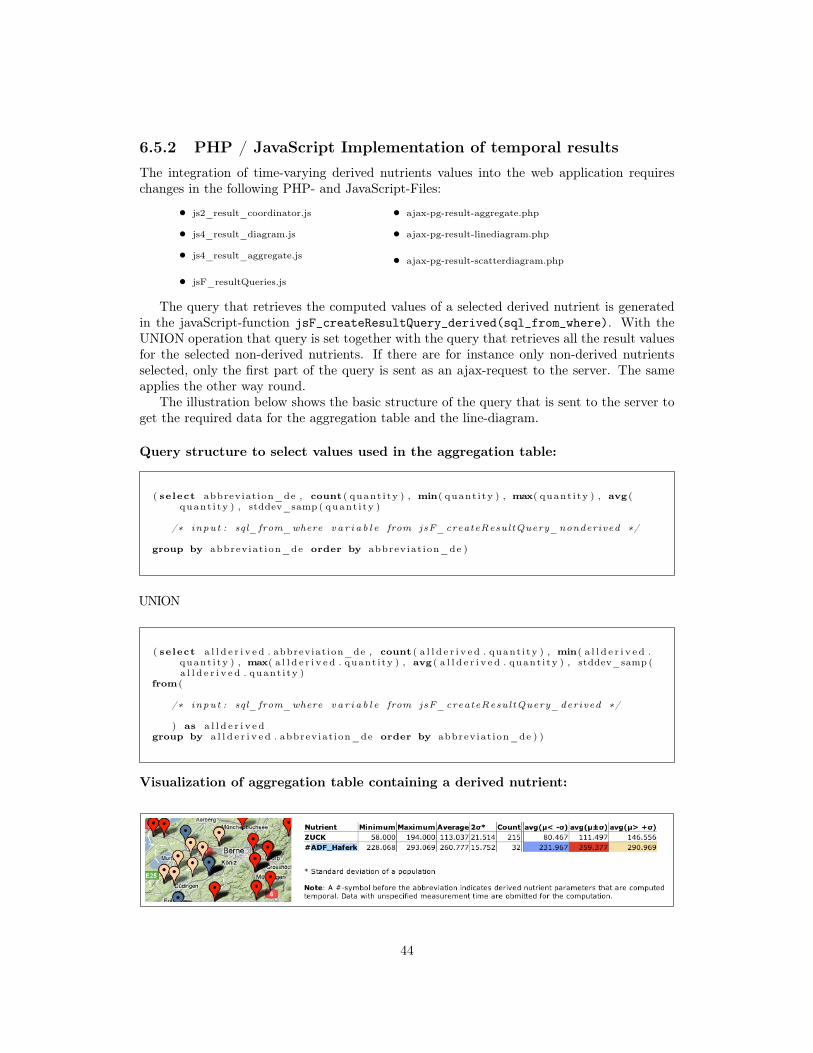
6.5.2 PHP / JavaScript Implementation of temporal results

The integration of time-varying derived nutrients values into the web application requireschanges in the following PHP- and JavaScript-Files:

• js2_result_coordinator.js

• js4_result_diagram.js

• js4_result_aggregate.js

• jsF_resultQueries.js

• ajax-pg-result-aggregate.php

• ajax-pg-result-linediagram.php

• ajax-pg-result-scatterdiagram.php

The query that retrieves the computed values of a selected derived nutrient is generatedin the javaScript-function jsF_createResultQuery_derived(sql_from_where). With theUNION operation that query is set together with the query that retrieves all the result valuesfor the selected non-derived nutrients. If there are for instance only non-derived nutrientsselected, only the first part of the query is sent as an ajax-request to the server. The sameapplies the other way round.

The illustration below shows the basic structure of the query that is sent to the server toget the required data for the aggregation table and the line-diagram.

Query structure to select values used in the aggregation table:

( select abbreviation_de , count ( quant i ty ) , min( quant i ty ) , max( quant i ty ) , avg (quant i ty ) , stddev_samp ( quant i ty )

/∗ input : sql_from_where var i a b l e from jsF_createResultQuery_nonderived ∗/

group by abbreviat ion_de order by abbreviat ion_de )

UNION

( select a l l d e r i v e d . abbreviation_de , count ( a l l d e r i v e d . quant i ty ) , min( a l l d e r i v e d .quant i ty ) , max( a l l d e r i v e d . quant i ty ) , avg ( a l l d e r i v e d . quant i ty ) , stddev_samp (a l l d e r i v e d . quant i ty )

from(

/∗ input : sql_from_where var i a b l e from jsF_createResultQuery_derived ∗/

) as a l l d e r i v e dgroup by a l l d e r i v e d . abbreviat ion_de order by abbreviat ion_de ) )

Visualization of aggregation table containing a derived nutrient:

44

Query structure to select values used in the line-diagram:

( ( select abbreviation_de , ( case when t_day i s null then to_date ( t_year | | ’−01−01 ’, ’YYYY−MM−DD’ ) else t_day end) as day , t_year , avg ( quant i ty )

/∗ input here : sql_from_where var i a b l e tha t i s generated injsF_createResultQuery_nonderived ∗/

) group by abbreviation_de , t_day , t_year order by abbreviation_de , day)

UNION

( ( select a l l d e r i v e d . abbreviation_de , to_date ( ( a l l d e r i v e d .day : : t ex t ) , ’YYYYMMDD’ )as t_day , null , avg ( a l l d e r i v e d . quant i ty )

from(

/∗ input here : sql_from_where var i a b l e tha t i s generated injsF_createResultQuery_derived ∗/

) as a l l d e r i v e dgroup by a l l d e r i v e d . abbreviation_de , t_day order by abbreviation_de , t_day )

Visualization of line-diagram/scatter-diagram containing a derived nutrient:

45

6.6 Compute derived nutrient values grouped by mea-

surement samples [Task 4]

6.6.1 Query

For the sample enlistment table, only values from the same meaurement sample are usedfor the computation. The listing below shows how the query can be defined to retrieve thedesired measurement values that are later used for the calculation.

Assume that we have a derived nutrient #ZUCK_FE containing the components ZUCKand FE. In this case and we want to list all the sample keys with the corresponding ZUCKand FE-Values. So, the formula can be calculated with the values that come from the samemeasurement sample. For that, the sample_key and an array with all the nutrient componentvalues that correspond to the sample_key is retrieved. Is there no ZUCK value or no FEvalue in a specific measurement sample, the sample_key is not retrieved. In case that thereare multiple measurement values of a nutrient in the same sample, the average of all thesevalues is taken.

Query that retrieves all the sample keys with their related ZUCK and FE value

1 select array [ZUCK. quantity , FE. quant i ty ] as values , sample_key2 from

3 ( select avg ( quant i ty ) as quantity , id_sample_fkey4 from d_nutrient ,56 /∗ i n s e r t here sql_from_where−Query according to s e l e c t e d opt ions ∗/78 fact_table , d_time , d_origin , d_quality_parameters , d_feed9 where id_time_fkey = time_key and id_or ig in_fkey = orig in_key and

id_qual ity_fkey = qual ity_key and id_feed_fkey = feed_key and (drying_condition_de in ( ’ b e l ü f t e t ’ ) ) and ( d_feed . name_de in ( ’Heu ’ ) ) and

nutrient_key=id_nutr ient_fkey and d_nutrient . abbreviat ion_de =’ZUCK’10 group by id_sample_fkey ) as ZUCK,111213 ( select avg ( quant i ty ) as quantity , id_sample_fkey14 from d_nutrient ,1516 /∗ i n s e r t here sql_from_where−Query according to s e l e c t e d opt ions ∗/1718 fact_table , d_time , d_origin , d_quality_parameters , d_feed19 where id_time_fkey = time_key and id_or ig in_fkey = orig in_key and

id_qual ity_fkey = qual ity_key and id_feed_fkey = feed_key and (drying_condition_de in ( ’ b e l ü f t e t ’ ) ) and ( d_feed . name_de in ( ’Heu ’ ) )

2021 and nutrient_key=id_nutr ient_fkey and d_nutrient . abbreviat ion_de =’FE ’22 group by id_sample_fkey ) as FE,2324 d_sample2526 where ZUCK. id_sample_fkey=sample_key and FE. id_sample_fkey=sample_key ;

• In the SELECT-clause of the query, the sample_key is retrieved with a correspondingarray that contain values for all the nutrient components for a specified derived nutrient.In the example above, the derived nutrient is composed of the nutrients ZUCK and FE.

• In addition to the relation d_sample that occurs in the FROM-clause, a temporarytable is defined for each involved component (line 3-10 and 13-22). In these subqueries,all the measurement values (quantity) that satisfy the restriction condition that areselected in the select part of the web application. Together with those measurmentvalues, the corresponding sample keys are retrieved.

46

• In the WHERE-clause, the join condition on the sample_key is set. So, all the valuesthat are retrieved as an array are measured in the same sample with the correspond-ing sample_key. With the help of an array as an attribute in the select clause, it isguaranteed that the query works for a various number of nutrient components.

In the next sub-chapter it is explained, how the described query is generated dynamicallydepending on the selections in the web application.

6.6.2 PL/pg SQL Function for sample results

The PL/pg sql function computederivedresults_bySamples(formula, sql_from_where)calculates derived nutrients values by using only measurement values that come from thesame measurement sample. As input parameter of this function acts the formula of a specificderived nutrient and the sql_from_where-Query that represents the selected options in theweb application. The main steps in these functions are listed as follows:

1. In a first step, all the abbreviations that are involved in a derived nutrient must be re-trieved. This is done with the help of the function getInvolvedAbbreviations(formula),which returns an array with all the abbreviations that are in the specified formula.

2. In a second step, a query as described in chapter 6.6.1 is generated. The retrieved resultof that query contains all the measurement values of the involved nutrient components,grouped by the sample_key. The listing below shows the generation of that query,where for each abbreviations in the array abbr[] , an additional part in the select-clause, from-clause, and where-clause is added.FOR n in array_lower ( abbr , 1) . . array_upper ( abbr , 1) LOOP

sq l_s e l e c t := sq l_s e l e c t | | ’ , ’ | | abbr [ n ] | | ’ . quant i ty ’ ;

sql_from := sql_from | |’ ( s e l e c t avg ( quant i ty ) as quantity , id_sample_fkeyfrom d_nutrient , ’

| | sql_from_where | |

’ and nutrient_key=id_nutr ient_fkey and d_nutrient . abbreviat ion_de= ’ | | ’ ’ ’ ’ | | abbr [ n ] | | ’ ’ ’ ’ | | ’

group by id_sample_fkey ) as ’ | | abbr [ n ] | | ’ , ’ ;sql_where := sql_where | | ’ and ’ | | abbr [ n ] | | ’ . id_sample_fkey=

sample_key ’ ;

end loop ;

sql_query := ’ s e l e c t array [ ’ | | substring ( sq l_se l e c t , 2 ) | | ’ ] as a ,sample_key

from ’ | | sql_from | | ’ d_sample ’ | |’ where ’ | | substring ( sql_where , 5) ;

3. Then, all the abbreviations of the formula are replaced with the measurement valuesfrom the query and the result of the expression is computed.

4. Finally, the function returns for each sample the result of the calculation and the cor-responding lims_number that refers to a specific sample_key.

47

6.6.3 PHP / JavaScript Implementation for sample results

The integration of derived nutrients values into the sample enlistment of the web page requireschanges in the following PHP- and JavaScript-Files:

• js2_result_coordinator.js

• jsF.resultQueries.js

• js3.result_list-map.js

• ajax-pg-result-google.php

The illustration below show how to basic structure of the query to retrieve the required datafor the sample enlistment. Again, the query is split in two parts:

1. In the first part, the measurement values for non-derived nutrients are retrieved,together with the corresponding lims_number and the nutrient abbreviation.

2. In the second part, the calculated values of derived nutrients are retrieved. Thelims_number that indicates the measurement sample is retrieved as well. The secondpart of the query is generated in jsF_createResultQuery_derived_bySamples().

Query structure to select values used in the sample enlistment:

( select dist inct lims_number , abbreviation_de , quant i ty

from

/∗ sql_from_where , created in jsD_CreateFromWhereQuery () ∗/

order by lims_number )

UNION

( select a l l d e r i v e d . lims_number , a l l d e r i v e d . abbreviation_de , a l l d e r i v e d . quant i tyas quant i ty

from(/∗ sql_derived_bySamples , created in jsF_createResultQuery_derived_bySamples (

sql_from_where ) ∗/

) as a l l d e r i v e d

order by abbreviation_de , lims_number )

Visualization of sample enlistment with a derived nutrient:

48

Chapter 7

Summary

In the preceding elaborations, some implementation methods for computing regressions forderived nutrients have been proposed. The focus of the project has been to find an effi-cient solution for computing derived nutrients as time-varying regressions. For that, differentapproaches have been described and implemented. Because of the performance problems de-scribed in chapter 5.2.3, the approach of using standard SQL to retrieve the computed valuesof derived nutrients could not be carried out successfully. In any case, an approach usingSQL views is not scalable. This means that it is not possible to compute time-varying valueson a variable data set that is selected by the user, because the data set has to be specified inthe view definition. That is why an alternative solution had to be found.

Finally, a number of algorithms were implemented as PL/pg SQL functions. The mostefficient approach, which involves using 3-dimensioal arrays (presented in chapter 5.5.2) wasthen used for the integration of derived nutrients into the current web application.

The adaption of the web application consisted of four main tasks, which are dividable intotwo main stages: After the changes of the update mechanism accoridng to the selection fieldshas been made, the methods that retrieve and display the result data have been adapted.

For derived nutrients, two different computation methods were integrated:

• First, the derived nutrient values are computed as time-varying regressions. The com-puted temporal result values are used for the representation of the line-diagramand the scatter-diagram. The aggregation values for displaying statistical informationabout a derived nutrient are computed by the same algorithm. With the help of the line-diagram, the derived nutrient values can be compared over time and historical analysesare possible.

• On the other hand, derived nutrients can be computed as sample result values.

These values are only calculated for measurement samples that contain data for eachcomponent involved in a formula. These values are integrated in the sample enlistmenton the left hand-side of the wep-page.

Both methods support the calculation of any type of formula that is composed of algebraicexpressions containing the most common mathematical operators. The PL/pg SQL functionhas been tested for some sample formulas of derived nutrients on the complete data set. Sofar, the web-application has been tested on a limited data set. Depending on the complexity ofthe formula and the number of tuples has to be retrieved and stored in memory, the executiontime can amount to several seconds.

49

An possible approach to the solution would be the development of a restriction condition,limiting the number of selectable derived nutrients. Otherwise, a potential execution time ofseveral seconds has to be put up.

An alternative and more efficient solution could be realized by computing the regressionresults for the historical representation in the same way as it is done in the sample enlistment.In that case, the derived nutrient values are computed only with data that exists within ameasurement sample. However, this would decrease the number of data values, limiting thesignificance of the results considerably. On the other hand, the use of the cost-intensive com-bining algorithm would not be needed, which would result in an improvement of performance.

50

Bibliography

[1] Agroscope Liebefeld-Posieux (2009). SchweizerischeFuttermitteldatenbank. URL: http://www.agroscope.admin.ch/futtermitteldatenbank/index.html?lang=de [Last access: 2011-11-13]

[2] Douglas, K., Dougklas S. (2003) PostgreSQL. A comprehensive guideto building, programming, and administering PostgreSQL databases.Sams Publishing. First Edition.

[3] Kemper, A. , Eickler, A. (2006). Datenbanksysteme: Eine Einführung.Oldenbourg Wissenschaftsverlag. 6. Auflage.

[4] Gupta A. , Mumick S. (1999). Materialized views techniques,implementations, and applications. MIT Press. First Edition.

[5] The PostgreSQL Global Development Group (2010). PostgreSQL 9.0.4Documentation. URL: http://www.postgresql.org/docs/9.0/interactive/index.html [Last access: 2011-11-20]

[6] Hitoshi, H. (2008). Window Functions for PostgreSQL DesignOverview. URL: http://umitanuki.net/pgsql/wfv08/design.html

[7] Worsley J., Drake J. (2002). Practical PostgreSQL. URL:http://www.linuxtopia.org/online_books/database_guides/Practical_PostgreSQL_database[Last access: 2011-11-20]

[8] Google (2011). Google chart tools. Collection of tutorial, examples andAPI library URL: http://code.google.com/intl/en/apis/chart/interactive/docs/index.html [Last access: 2011-11-22]

[9] Elmasri R., Navathe S. (2004). Fundamentals of Database Systems.Pearson Education. Fourth Edition.

51

Documents

Managing and Querying Derived Nutrient Parameters in the