Frontiers + Innovation – 2009 CSPG CSEG CWLS Convention 376

Making FX Interpolation More Robust by Spectrum-guided Reconstruction Mostafa Naghizadeh* and Mauricio Sacchi

University of Alberta, Edmonton, Alberta, Canada mostafan@ualberta.ca , msacchi@ualberta.ca

Summary In this paper the spectrum of prediction filters is used to find a region of support (in the wavenumber domain) in order to reconstruct irregularly missing traces. The region of support is determined by identifying the location of peaks in the spectrum of prediction filters. The proposed method brings further improvements for the reconstruction of large gaps in data, high percentage of missing traces, and extrapolation of data in comparison to the application of prediction filters in the space domain. Synthetic and real data examples are provided to present the advantages of the proposed method.

Introduction Spitz (1991) showed how one could extract prediction filters from spatial data at low frequencies to reconstruct aliased spatial data. Naghizadeh and Sacchi (2007) extended the method to the case of data on a regular grid but with irregular distribution of traces on the grid. The latter is named Multi-Step Auto-Regressive (MSAR) reconstruction. The MSAR reconstruction method is a combination of a Fourier reconstruction method (Sacchi and Liu, 2004) and f-x interpolation (Spitz, 1991). MSAR can be summarized as follows:

1) The low frequency (unaliased) portion of data is reconstructed using Minimum Weighted Norm Interpolation (MWNI) (Liu and Sacchi, 2004).

2) Prediction filters of all frequencies are extracted from an already regularized low frequency spatial data.

3) The estimated prediction filters are used to reconstruct the missing spatial samples in the aliased portion of the spectrum.

Stages 1) and 2) are the estimation stages and 3) is the reconstruction stage. In this paper we propose a new and robust method to solve the reconstruction stage. In the original formulation of MSAR the reconstruction stage uses prediction filters harvested from low frequencies to reconstruct spatial data in the aliased band (Spitz, 1991). In this article we propose to use the spectrum of the prediction filters to define a region of spectral support. Once the region of spectral support (areas of unaliased energy in the f-k plane) is defined we turn the reconstruction problem into a simple Fourier reconstruction algorithm that solves for unknown spectral components using the least-squares method (Duijndam et al., 1999). We illustrate with synthetic examples that the proposed method can handle gaps and extrapolation problems much better than our original formulation of MSAR.

Data reconstruction using the spectrum of prediction filters

Let ),( fxd h represent data in the f-x domain where hx indicates the given spatial positions. Suppose that a small band of low frequencies from ],[ maxmin fff ∈ has been regularized and we have access to equally

Frontiers + Innovation – 2009 CSPG CSEG CWLS Convention 377

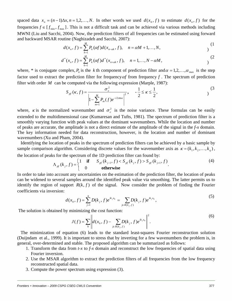
spaced data .,,2,1,)1( Nnxnxn K=Δ−= In other words we used ),( fxd h to estimate ),( fxd n for the frequencies ],[ maxmin fff ∈ . This is not a difficult task and can be achieved via various methods including MWNI (Liu and Sacchi, 2004). Now, the prediction filters of all frequencies can be estimated using forward and backward MSAR routine (Naghizadeh and Sacchi, 2007):

∑=

− +==M

kknkn NMnfxdfPfxd

1,,,1),,()(),( Kαα α

(1)

∑=

+ −==M

kknkn MNnfxdfPfxd

1

** ,,,1),,()(),( αα α K (2

)

where, * is conjugate complex, kP is the k th component of prediction filter and max,,2,1 αα K= is the step factor used to extract the prediction filter for frequency fα from frequency f . The spectrum of prediction filter with order M can be computed via the following expression (Marple, 1987):

,21

21

)(1

),( 2

1

2

2

≤≤

−

=

∑=

−

κσ

κκπ

ε - ,M

m

mim

pf

efP

fS (3

)

where, κ is the normalized wavenumber and 2εσ is the noise variance. These formulas can be easily

extended to the multidimensional case (Kumaresan and Tufts, 1981). The spectrum of prediction filter is a smoothly varying function with peak values at the dominant wavenumbers. While the location and number of peaks are accurate, the amplitude is not a direct estimate of the amplitude of the signal in the f-x domain. The key information needed for data reconstruction, however, is the location and number of dominant wavenumbers (Xu and Pham, 2004).

Identifying the location of peaks in the spectrum of prediction filters can be achieved by a basic sample by sample comparison algorithm. Considering discrete values for the wavenumber axis as ),,,( 21 qkkk K=κ , the location of peaks for the spectrum of the 1D prediction filter can found by:

⎩⎨⎧ ><

=Λ +− .0

),(),(),(1),( 11

otherwise if fkSfkSfkS

fk jpfjpfjpfjpf

(4)

In order to take into account any uncertainties on the estimation of the prediction filter, the location of peaks can be widened to several samples around the identified peak value via smoothing. The latter permits us to identify the region of support ),( fkR of the signal. Now consider the problem of finding the Fourier coefficients via inversion:

,),(),(),(),(1

∑∑∈=

==fkRj

xikj

q

j

xikjh

j

hjhj efkDefkDfxd (5)

The solution is obtained by minimizing the cost function:

.),(),()(2

),(∑ ∑

∈

−=h fkRj

xikjh

j

hjefkDfxdfJ (6)

The minimization of equation (6) leads to the standard least-squares Fourier reconstruction solution (Duijndam et al., 1999). It is important to stress that by inverting for a few wavenumbers the problem is, in general, over-determined and stable. The proposed algorithm can be summarized as follows:

1. Transform the data from t-x to f-x domain and reconstruct the low frequencies of spatial data using Fourier inversion.

2. Use the MSAR algorithm to extract the prediction filters of all frequencies from the low frequency reconstructed spatial data.

3. Compute the power spectrum using expression (3).

Frontiers + Innovation – 2009 CSPG CSEG CWLS Convention 378

4. Identify the location of spectral peaks and define the region of support ),( fkR . 5. Solve Equation (6) to find ),( fkD . 6. Use the inverse Fourier to transform ),( fkD to ),( fxd n . 7. Transform the f-x data to the t-x domain.

Examples Figure 1a shows an example of a sampling function composed of a decimation process as well as a gap. Figure 1e shows the f-k panel of Figure 1a. The decimation process causes overlapped repetition of the spectrum of the original data and the existence of a gap in the middle of the section produces a small artifact around the spectrum of the decimated data. Figures 1b, 1c, and 1d show the reconstructed data using MWNI, MSAR (original formulation), and MSAR with the reconstruction stage proposed in this paper, respectively. The f-k panel of Figures 1b, 1c, and 1d are depicted in Figures 1f, 21g, and 1h, respectively. It is interesting that MWNI is only able to recover the decimated data and still can not fill the regularly missing traces. Meanwhile, the ordinary MSAR method successfully fills the decimated data outside the gap area but struggles to recover the data at the gap location. However, when MSAR is used to define regions of spectral support, the method overcomes the shortcoming seen in Figures 1b and 1c. The spectrum of prediction filter and the region of support are shown in Figure 2 for the normalized frequency 0.3.

Figure 1: a) Section of missing traces. b), c), and d) are the reconstruction of (a) using the MWNI, MSAR, and MSAR with the new proposed reconstruction, respectively. e), f), g), and h) are the f-k panel of a, b, c, and d, respectively.

Figure 2: Spectrum of prediction filter (Solid line with solid circles) and region

of spectral support (dashed line) for the normalized frequency 0.3.

Frontiers + Innovation – 2009 CSPG CSEG CWLS Convention 379

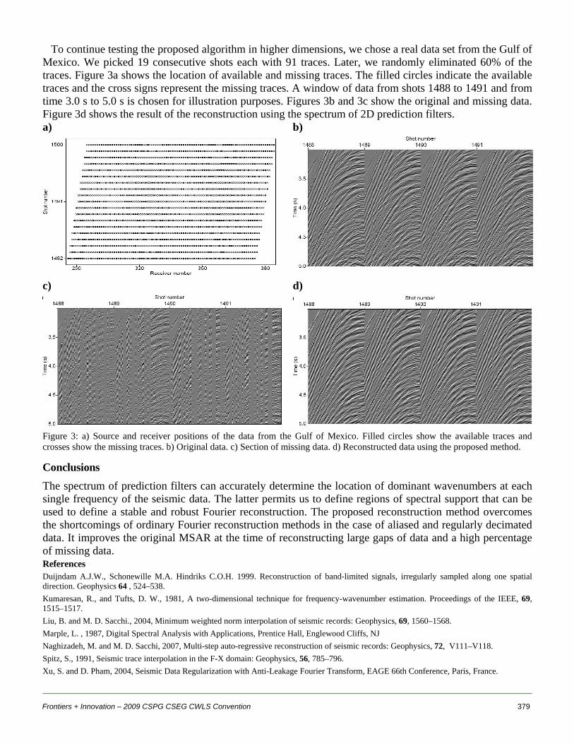
To continue testing the proposed algorithm in higher dimensions, we chose a real data set from the Gulf of Mexico. We picked 19 consecutive shots each with 91 traces. Later, we randomly eliminated 60% of the traces. Figure 3a shows the location of available and missing traces. The filled circles indicate the available traces and the cross signs represent the missing traces. A window of data from shots 1488 to 1491 and from time 3.0 s to 5.0 s is chosen for illustration purposes. Figures 3b and 3c show the original and missing data. Figure 3d shows the result of the reconstruction using the spectrum of 2D prediction filters. a) b)

c) d)

Figure 3: a) Source and receiver positions of the data from the Gulf of Mexico. Filled circles show the available traces and crosses show the missing traces. b) Original data. c) Section of missing data. d) Reconstructed data using the proposed method.

Conclusions The spectrum of prediction filters can accurately determine the location of dominant wavenumbers at each single frequency of the seismic data. The latter permits us to define regions of spectral support that can be used to define a stable and robust Fourier reconstruction. The proposed reconstruction method overcomes the shortcomings of ordinary Fourier reconstruction methods in the case of aliased and regularly decimated data. It improves the original MSAR at the time of reconstructing large gaps of data and a high percentage of missing data. References Duijndam A.J.W., Schonewille M.A. Hindriks C.O.H. 1999. Reconstruction of band-limited signals, irregularly sampled along one spatial direction. Geophysics 64 , 524–538. Kumaresan, R., and Tufts, D. W., 1981, A two-dimensional technique for frequency-wavenumber estimation. Proceedings of the IEEE, 69, 1515–1517. Liu, B. and M. D. Sacchi., 2004, Minimum weighted norm interpolation of seismic records: Geophysics, 69, 1560–1568. Marple, L. , 1987, Digital Spectral Analysis with Applications, Prentice Hall, Englewood Cliffs, NJ Naghizadeh, M. and M. D. Sacchi, 2007, Multi-step auto-regressive reconstruction of seismic records: Geophysics, 72, V111–V118. Spitz, S., 1991, Seismic trace interpolation in the F-X domain: Geophysics, 56, 785–796. Xu, S. and D. Pham, 2004, Seismic Data Regularization with Anti-Leakage Fourier Transform, EAGE 66th Conference, Paris, France.