1

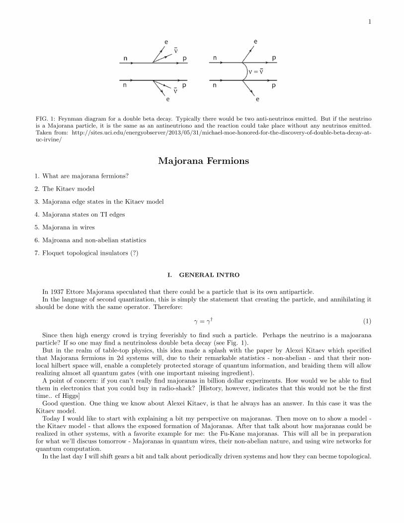
FIG. 1: Feynman diagram for a double beta decay. Typically there would be two anti-neutrinos emitted. But if the neutrinois a Majorana particle, it is the same as an antineutriono and the reaction could take place without any neutrinos emitted.Taken from: http://sites.uci.edu/energyobserver/2013/05/31/michael-moe-honored-for-the-discovery-of-double-beta-decay-at-uc-irvine/

Majorana Fermions

1. What are majorana fermions?

2. The Kitaev model

3. Majorana edge states in the Kitaev model

4. Majorana states on TI edges

5. Majorana in wires

6. Majroana and non-abelian statistics

7. Floquet topological insulators (?)

I. GENERAL INTRO

In 1937 Ettore Majorana speculated that there could be a particle that is its own antiparticle.In the language of second quantization, this is simply the statement that creating the particle, and annihilating it

should be done with the same operator. Therefore:

γ = γ† (1)

Since then high energy crowd is trying feverishly to find such a particle. Perhaps the neutrino is a majoaranaparticle? If so one may find a neutrinoless double beta decay (see Fig. 1).But in the realm of table-top physics, this idea made a splash with the paper by Alexei Kitaev which specified

that Majorana fermions in 2d systems will, due to their remarkable statistics - non-abelian - and that their non-local hilbert space will, enable a completely protected storage of quantum information, and braiding them will allowrealizing almost all quantum gates (with one important missing ingredient).A point of concern: if you can’t really find majoranas in billion dollar experiments. How would we be able to find

them in electronics that you could buy in radio-shack? [History, however, indicates that this would not be the firsttime.. cf Higgs]Good question. One thing we know about Alexei Kitaev, is that he always has an answer. In this case it was the

Kitaev model.Today I would like to start with explaining a bit my perspective on majoranas. Then move on to show a model -

the Kitaev model - that allows the exposed formation of Majoranas. After that talk about how majoranas could berealized in other systems, with a favorite example for me: the Fu-Kane majoranas. This will all be in preparationfor what we’ll discuss tomorrow - Majoranas in quantum wires, their non-abelian nature, and using wire networks forquantum computation.In the last day I will shift gears a bit and talk about periodically driven systems and how they can becme topological.

2

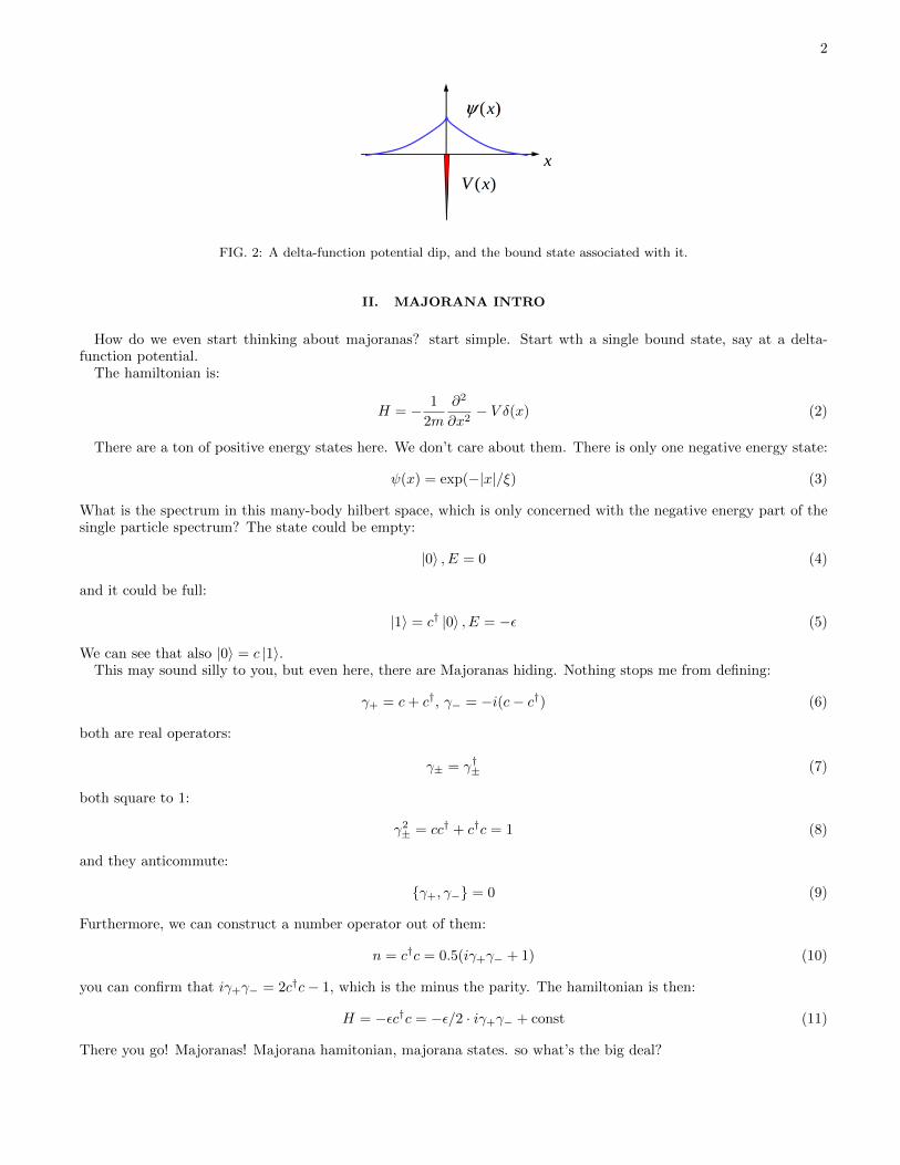
FIG. 2: A delta-function potential dip, and the bound state associated with it.

II. MAJORANA INTRO

How do we even start thinking about majoranas? start simple. Start wth a single bound state, say at a delta-function potential.The hamiltonian is:

H = − 1

2m

∂2

∂x2− V δ(x) (2)

There are a ton of positive energy states here. We don’t care about them. There is only one negative energy state:

ψ(x) = exp(−|x|/ξ) (3)

What is the spectrum in this many-body hilbert space, which is only concerned with the negative energy part of thesingle particle spectrum? The state could be empty:

|0� , E = 0 (4)

and it could be full:

|1� = c† |0� , E = −� (5)

We can see that also |0� = c |1�.This may sound silly to you, but even here, there are Majoranas hiding. Nothing stops me from defining:

γ+ = c+ c†, γ− = −i(c− c†) (6)

both are real operators:

㱠= ㆱ (7)

both square to 1:

γ2± = cc† + c†c = 1 (8)

and they anticommute:

{γ+, γ−} = 0 (9)

Furthermore, we can construct a number operator out of them:

n = c†c = 0.5(iγ+γ− + 1) (10)

you can confirm that iγ+γ− = 2c†c− 1, which is the minus the parity. The hamiltonian is then:

H = −�c†c = −�/2 · iγ+γ− + const (11)

There you go! Majoranas! Majorana hamitonian, majorana states. so what’s the big deal?

3

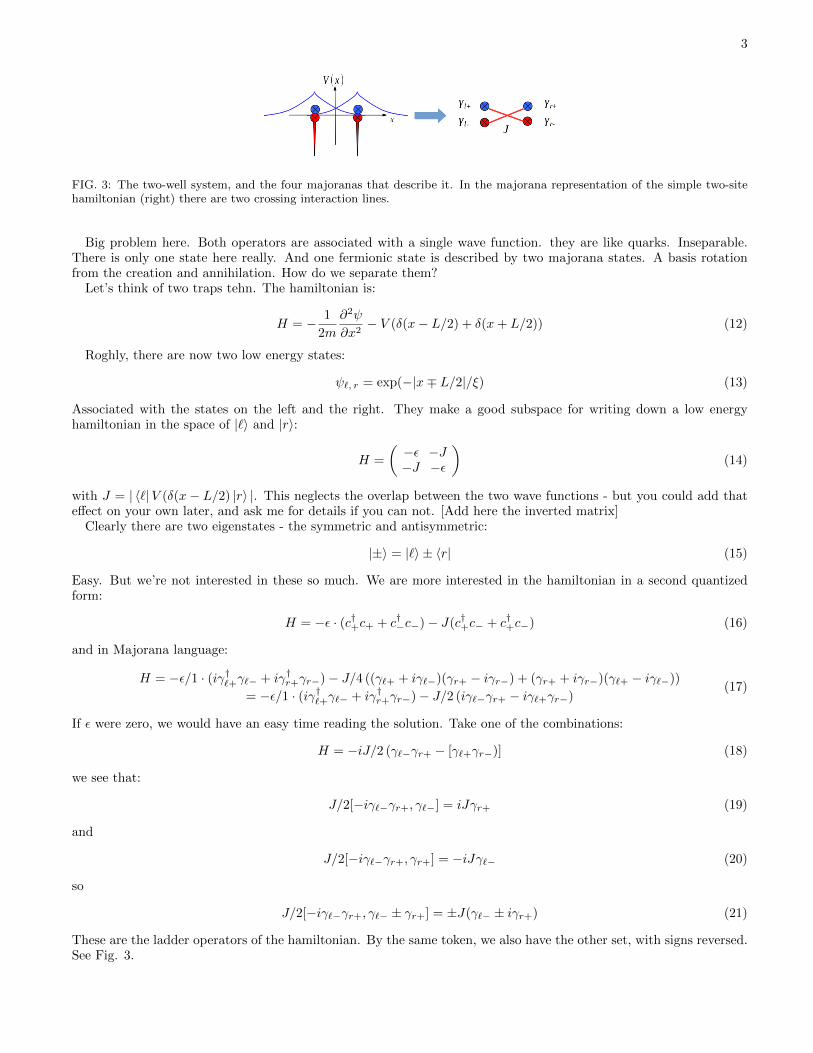
FIG. 3: The two-well system, and the four majoranas that describe it. In the majorana representation of the simple two-sitehamiltonian (right) there are two crossing interaction lines.

Big problem here. Both operators are associated with a single wave function. they are like quarks. Inseparable.There is only one state here really. And one fermionic state is described by two majorana states. A basis rotationfrom the creation and annihilation. How do we separate them?Let’s think of two traps tehn. The hamiltonian is:

H = − 1

2m

∂2ψ

∂x2− V (δ(x− L/2) + δ(x+ L/2)) (12)

Roghly, there are now two low energy states:

ψ�, r = exp(−|x∓ L/2|/ξ) (13)

Associated with the states on the left and the right. They make a good subspace for writing down a low energyhamiltonian in the space of |�� and |r�:

H =

�−� −J−J −�

�(14)

with J = | ��|V (δ(x− L/2) |r� |. This neglects the overlap between the two wave functions - but you could add thateffect on your own later, and ask me for details if you can not. [Add here the inverted matrix]Clearly there are two eigenstates - the symmetric and antisymmetric:

|±� = |��± �r| (15)

Easy. But we’re not interested in these so much. We are more interested in the hamiltonian in a second quantizedform:

H = −� · (c†+c+ + c†−c−)− J(c†+c− + c†+c−) (16)

and in Majorana language:

H = −�/1 · (iγ†�+γ�− + iγ†

r+γr−)− J/4 ((γ�+ + iγ�−)(γr+ − iγr−) + (γr+ + iγr−)(γ�+ − iγ�−))= −�/1 · (iγ†

�+γ�− + iγ†r+γr−)− J/2 (iγ�−γr+ − iγ�+γr−)

(17)

If � were zero, we would have an easy time reading the solution. Take one of the combinations:

H = −iJ/2 (γ�−γr+ − [γ�+γr−)] (18)

we see that:

J/2[−iγ�−γr+, γ�−] = iJγr+ (19)

and

J/2[−iγ�−γr+, γr+] = −iJγ�− (20)

so

J/2[−iγ�−γr+, γ�− ± γr+] = ±J(γ�− ± iγr+) (21)

These are the ladder operators of the hamiltonian. By the same token, we also have the other set, with signs reversed.See Fig. 3.

4

FIG. 4: The necessary magic trick for getting a majorana

FIG. 5: The kitaev chain. As if one of the majorana interactions are missing in each bond. There are two edge majoranas thatare decoupled if � = 0.

A. Kitaev’s magic trick

What is our goal? We want to be able to take these majoranas - two for a state - and bring them apart. How canwe break such an integral object? The two majoranas belong to a single state! We need something like Fig. 4. . .We do habe a magician, though. Kitaev said - what about just removing one of the interaction lines in the two site

problem? Let’s make the model into a chain, and let’s not have the two couplings between the majoranas - let’s justhave a linked chain.This would be the following model:

H =1

2

�

i

�−i�γi+γi− − iJγi+γ(i+1)−

�(22)

Why is this magic? Check this out. set � = 0. The Majoranas are now disconnected. We can find the eigen creationand annihilation operators in each bond:

di = γi+ + iγ(i+1)−, d†i = γi+ − iγ(i+1)− (23)

But this leaves a set of two zero modes on the two sides. left and right:

[H, γ0−] = [H, γL+] = 0 (24)

Two majorana edge modes! Thi is clearly not the case if we have J = 0, and � > 0. Then each site is left to itsown, and there are no zero modes. . . These two points we discussed are simply speaking the example points of thetopological and trivial pahse of the kitaev model.

B. Kitaev model for electrons

What is the model in terms of the original electrons? We need to key in the majorana definitions int he hamiltonain26. not hard to do, with:

ci =1

2(γi+ + iγi−) , c

†i =

1

2(γi+ − iγi−) (25)

And we get:

HK =�

i

�−�c†i ci −

J

2(ci+1 − c†i+1)(ci + c†i )

�=

�

i

�−�c†i ci −

J

2(c†i+1ci + c†i ci) +

Δ

2(ci+1ci + c†i c

†i+1)

�(26)

5

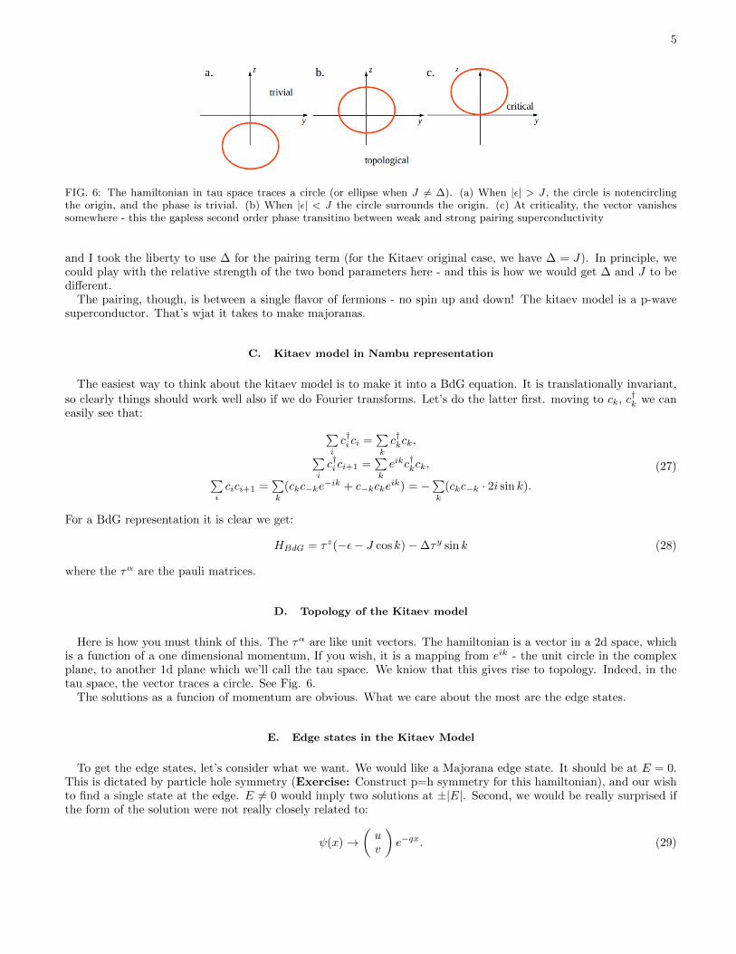
FIG. 6: The hamiltonian in tau space traces a circle (or ellipse when J �= Δ). (a) When |�| > J , the circle is notencirclingthe origin, and the phase is trivial. (b) When |�| < J the circle surrounds the origin. (c) At criticality, the vector vanishessomewhere - this the gapless second order phase transitino between weak and strong pairing superconductivity

and I took the liberty to use Δ for the pairing term (for the Kitaev original case, we have Δ = J). In principle, wecould play with the relative strength of the two bond parameters here - and this is how we would get Δ and J to bedifferent.The pairing, though, is between a single flavor of fermions - no spin up and down! The kitaev model is a p-wave

superconductor. That’s wjat it takes to make majoranas.

C. Kitaev model in Nambu representation

The easiest way to think about the kitaev model is to make it into a BdG equation. It is translationally invariant,

so clearly things should work well also if we do Fourier transforms. Let’s do the latter first. moving to ck, c†k we can

easily see that:

�i

c†i ci =�k

c†kck,�i

c†i ci+1 =�k

eikc†kck,�i

cici+1 =�k

(ckc−ke−ik + c−kcke

ik) = −�k

(ckc−k · 2i sin k).(27)

For a BdG representation it is clear we get:

HBdG = τz(−�− J cos k)−Δτy sin k (28)

where the τα are the pauli matrices.

D. Topology of the Kitaev model

Here is how you must think of this. The τα are like unit vectors. The hamiltonian is a vector in a 2d space, whichis a function of a one dimensional momentum, If you wish, it is a mapping from eik - the unit circle in the complexplane, to another 1d plane which we’ll call the tau space. We kniow that this gives rise to topology. Indeed, in thetau space, the vector traces a circle. See Fig. 6.The solutions as a funcion of momentum are obvious. What we care about the most are the edge states.

E. Edge states in the Kitaev Model

To get the edge states, let’s consider what we want. We would like a Majorana edge state. It should be at E = 0.This is dictated by particle hole symmetry (Exercise: Construct p=h symmetry for this hamiltonian), and our wishto find a single state at the edge. E �= 0 would imply two solutions at ±|E|. Second, we would be really surprised ifthe form of the solution were not really closely related to:

ψ(x) →�

uv

�e−qx. (29)

6

The boundary condition should be ψ = 0 at the edge. In lattice models this is essentially always the case for localizedmid-gap states.This makes our job somewhat easy. Step one: replace eik → e−q. Step two - solve for e−q. Step three: see if you

can fulfill boundary conditions. This gives:

H → τz(−�− J

2(eq + q−q)) + i

Δ

2τy(e

−q − eq) (30)

We want to find zero solutions of this, so some q where H2 = 0. Actually, looking at the hamiltonian, I was going tosuggest squaring it - the τ ’s either square to 1 or kill eachother due to anticommutation. We get:

�+ J cosh q = ±Δ sinh q (31)

This already looks like we are going to get more than one solution. Which solutions would we need?Which is legit? The only way we can get ψ = 0 boundary condition satisfied, is if we had two solutions that had

the same eigenvector in the kernel of H:

ψ =

�uv

�(e−q1x − e−q2x) (32)

Looking back it seems that we can have two types of hamiltonians depending on the sign we choose for the first squareroot:

τz ± iτy =

�1 ±1

±(−1) −1

�(33)

Both possibilities are fine. They have the solutions (respectively):

�1∓1

�(34)

as an eigenvector that makes them vanish. Good sign! We eant a majorana, and what are these amplitudes if notthe coefficients of c and c†, and therefore add up to something reasonable and real (or pure imaginary, whch is easyto rectify). Then, for each choice of a sign, we want two solutions for e−q that are smaller than 1. So let’s make thechoice of + in eq. (31). and:

e−2q(J +Δ) + 2e−q�+ (J −Δ) = 0 (35)

Easy to solve:

e−q =−�±

��2 − (J2 −Δ2)

(J +Δ)(36)

We see that there are only two such solutions that are smaller than 1 when � < J . We can just dial in � = J , andimmediately we get:

e−q =−J ±Δ

J +Δ(37)

So one of the solutions is 1.If you were in doubt regarding the boundary condition, here is the explanation. The reason for the homogeneous

boundary conditions is really that we are trying to diagonalize a hamiltonian with no translation invariance using theeigenstates of a uniform problem. We can do it - as long as we find a combination that satisfies the right boundaryconditions. The wave function should not venture to places where there is no lattice.Exercises:

1. Find edge states for a domain wall between Δ and Δeiφ. These states are complicated and will not lie at E = 0,so assume � = 0 for this to makes things simple. What is E(φ)?

2. Find an edge state of the kitaev model between two domains - one topological with � = 0 and the other with � = 4J .Assume Δ = 2J .

7

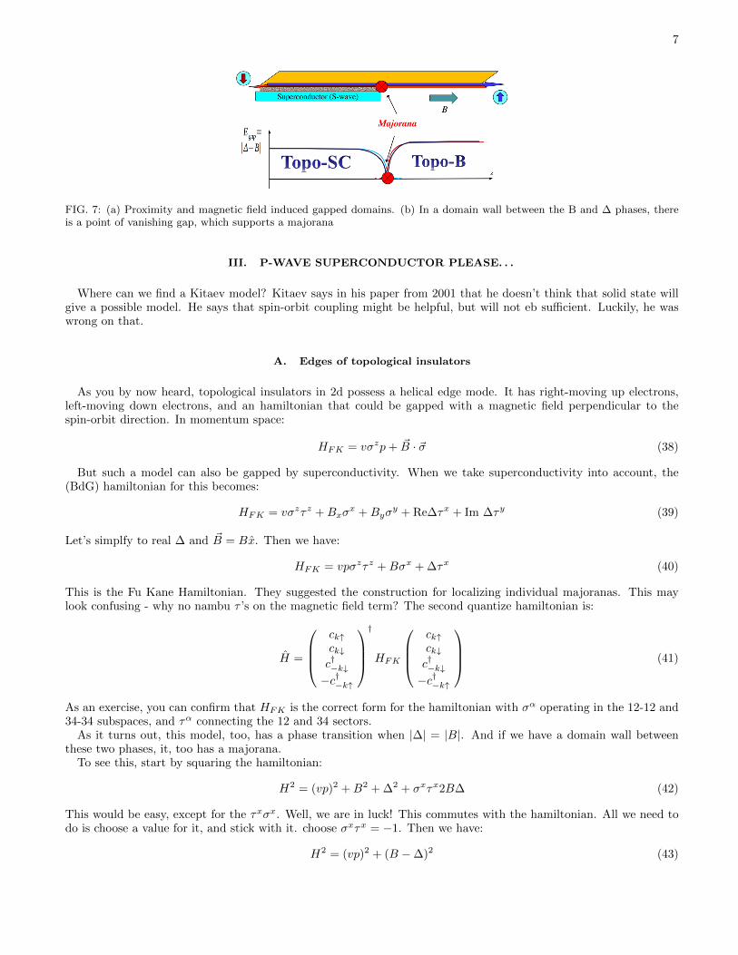
FIG. 7: (a) Proximity and magnetic field induced gapped domains. (b) In a domain wall between the B and Δ phases, thereis a point of vanishing gap, which supports a majorana

III. P-WAVE SUPERCONDUCTOR PLEASE. . .

Where can we find a Kitaev model? Kitaev says in his paper from 2001 that he doesn’t think that solid state willgive a possible model. He says that spin-orbit coupling might be helpful, but will not eb sufficient. Luckily, he waswrong on that.

A. Edges of topological insulators

As you by now heard, topological insulators in 2d possess a helical edge mode. It has right-moving up electrons,left-moving down electrons, and an hamiltonian that could be gapped with a magnetic field perpendicular to thespin-orbit direction. In momentum space:

HFK = vσzp+ �B · �σ (38)

But such a model can also be gapped by superconductivity. When we take superconductivity into account, the(BdG) hamiltonian for this becomes:

HFK = vσzτz +Bxσx +Byσ

y +ReΔτx + Im Δτy (39)

Let’s simplfy to real Δ and �B = Bx. Then we have:

HFK = vpσzτz +Bσx +Δτx (40)

This is the Fu Kane Hamiltonian. They suggested the construction for localizing individual majoranas. This maylook confusing - why no nambu τ ’s on the magnetic field term? The second quantize hamiltonian is:

H =

ck↑ck↓c†−k↓−c†−k↑

†

HFK

ck↑ck↓c†−k↓−c†−k↑

(41)

As an exercise, you can confirm that HFK is the correct form for the hamiltonian with σα operating in the 12-12 and34-34 subspaces, and τα connecting the 12 and 34 sectors.

As it turns out, this model, too, has a phase transition when |Δ| = |B|. And if we have a domain wall betweenthese two phases, it, too has a majorana.To see this, start by squaring the hamiltonian:

H2 = (vp)2 +B2 +Δ2 + σxτx2BΔ (42)

This would be easy, except for the τxσx. Well, we are in luck! This commutes with the hamiltonian. All we need todo is choose a value for it, and stick with it. choose σxτx = −1. Then we have:

H2 = (vp)2 + (B −Δ)2 (43)

8

Indeed gaplessness at the point of crossing. And a gap Egap = |B − Δ| in general. But how to see the majorana?Here is a neat way. Let’s have:B = Δ+ bx. Also, note that if we know that σxτx = −1 we also know that τx = −σx.So:

HFK → pvσzτz + (B(x)−Δ)σx = pvσzτz + bxσx (44)

To some of you this will look familiar. It has the same structure as Landau levels in a Dirac cone. What do we knowabout LL’s in a Dirac cone? They have a zero mode. Square the hamiltonian, and what do you get?

H2FK = v2p2 + b2x2 + vbiσyτz[p, x] (45)

The eigenvalues of the first operator are known: (n + 1/2)ω = (n + 1/2)√2v2 · 2b2 = (2n + 1)vb. The second term

has an operator on it. No fear - it commutes with σxτx, so we can diagonalize it too. Guess what - it is either plusor minus 1.So:

E2 = (2n+ 1)vb± vb (46)

n = 0 and the minus choice gives a zero mode. It is a majorana mode - easy to see. Not hard to figure out that allother states are the E = ±

�(2m)vb, with m integer.

B. Majorana wires

You would think that topological edges are good enough. You are almost right. But they are hard to handle, hardto fabricate outside Leiden, and maybe also Rice, and they are very hard to put in proximity to a superconductor.You could think of 2d systems in general, but ultimately there will always be complications. The was one insight fromtwo dimensions that came from Jay Say, Roman Lutchyn and Sankar Das Sarma, and also from Jason Alicea: Usespin orbit in regular wells. With α describing Rashba coupling, and β describing the Dresselhaus coupling, we have:

H2 = p2/2m+ (pxσy − pyσ

x)α+ βpxσz (47)

This could be gapped with a B field perpendicular to the plane in the case of just Rashba, and parallel to the planein the case of a dominant Dresselhaus interaction in [110] growth direction, and also with a superconductor. Themagnetic field essentially eliminates one spin flavor, and the superconductor makes for a p-wave superconductor. Thecore of vortex in the superconductor will have a Majorana.But moving vortices is hard. We want wires.To realize Majoranas in quantum wires we need semiconducting wires with strong spin orbit: InAs or SbTe were

the examples that came to our minds, then we almost get the edge states of the topolgoical insulators:

H = p2/2m+ σzλp (48)

At low momenta, this is nothing but the topological insulator helical edge. Further away, at high momenta, thereare additinal states near energy E = 0 which we need to care about. Problem. But this problem has a very simplesolution. Gap the whole thing with a superconductor. See Fig. 8.Just as before, we can dress this with a pairing, and upgrade to a nambu representation:

H = τz(p2/2m− µ+ pvσz) +Bσx +Δτx (49)

And nothing much is changed frm the case of the topological insulator. When B = Δ the k=0 piece has a gaplesspoint, and a phase transition, while the high memontum regions are still gapped. Interestingly, hre we can tune apahse transition in terms of chemical potential. At p = 0, we see that

H = −µτ z +Bσx +Δτx (50)

The eigenvalues of this hamiltonian are clear:

E = ±B ± (µ2 +Δ2) (51)

so now the phase transition occurs at µ2 +Δ2 = B, by and large.Majorana states appear either at the edge of a wire in the topological phases, or in domain walls, as in Fig. 9.

9

FIG. 8: (a) A wire with proximity to a superconductor, a magnetic field, and a series of gates. (b) Dispersion of a spin-orbitcoupled wire.

FIG. 9: A domain wall between the two phases of the majorana-supporting quantum wires could be tuned using a space-dependent chemical potentials. This could be achieved by an array of individually controlled gates, and a chemical potentialthat depends on space.

In fact, this model becomes the Kitaev model, pretty much at the limit of high magnetic field. Think of the limitof B ∼ µ � mλ2. In this case only the down spins survive. Without superconductivity we have:

H =p2

2m+ vp�e · �σ +Bσz (52)

assuming that B is large, the wave function in the lower band would be:

Ψ(x) =

�α1

�eipx (53)

Doing first order perturbation theory we see that

α ∼ vp(ex − iey)

2B(54)

Substituting this into the Hamiltonian with pairing we have:

H = (p2

2m− µ−B)c†pcp +Δ

vp(ex − iey)

2Bcpc−p +H.C. (55)

This is the continuoum limit of the Kitaev model.Generally speaking, the penetration length of the majorana states will be given as v/hEgap.The leaders in realizing majoranas in such wires are Leo Kouwenhoven, Moti Heiblum, and Charlie Marcus. It

is interesting to note what the relevant parameters are for the wires. Marcus managed to obtain hard gaps of the

10

FIG. 10: Each majorana fermion has a branch cut, and when other majorana cross it, their operator gets a minus sign. Uponexchange this happens only to one majorana, but a full braid will make both majoranas have a minus sign. Contrast this withregular fermions, for which an exchange produces a minus sign, and a braid returns the state to its original phase.

order of 2K in InAs wires. Kouwenhoven measured spin orbit coupling of upto 1eV A, which correspond to 105m/sspin-orbit velocity in InSb. The g factors of the wires vary depending on wire thickness and can rage from 2 to 30,presumably.

C. Majorana in iron chains

A recent development, which I had not fully digested yet, is the realization of the same model as the wires byplacing a chain of iron atoms on lead superconductors. The lead is heavy - hence spin orbit. The iron is magnetic -hence the Zeeman field. It is sitting atop a superconductor. Seems like all ingredients are there. So far reported aregaps of order 0.1meV and a remarkably short decay length. Authors to follow: Yazdani and Bernevig’s group for thediscovery and initial picture, and von Oppen and Glazman for the more detailed explanation.

IV. MAJORANAS AND QUANTUM COMPUTATION

A. Majorana statistics

What makes maojranas so coveted? They are nonabelian anyons. Let’s cosider two separated majoranas swimmingin an ocean of p-wave superconductivity. call them γA and γB . First off, you can store information in them in a reallynon-local way. The parity of the two majoranas can encode information (although not yet quantum). The hilbertspace, as you may recall is:

|0� , |1� = 1

2(γA + iγB) |0� (56)

This is amazing - since the information about the parity is not in one place or the other. It is everywhere. If the twomajoranas are far from eachother, then nothing local can actually detect their state. This is the point that Kitaevmade. Remember?Each majorana operator is made out of fermions. And fermions have to get a −1 upon exchange. This −1 could be

facilitated by thinking of a branch cut - a string that stretches from each fermionic entity, and when other fermioniccross it, they get slapped with the −1. If we have a full braid - then each fermion will get a -1, and overall, the wavefunction will remain invariant.With majoranas it becomes more complex. Literally. Now instead of electrons think of the majoranas. Upon

exchange, γB goes through the string of γA, but not vice versa. Then they replace each other: γA → −γB andγB → γA. For the Hilbert space above, the operator γA + iγB is of extreme importance:

γA + iγB → −γB + iγA = i(γA + iγB) (57)

hmm. . . the state just got slapped a in factor, with n the occupation, 0 or 1. Do it again, and one gets (−1)n. Thisway of doing this follows from Ivanov’s “Non-abelian statistics of half-quantum vortices in p-wave superconductors”,D. A. Ivanov, Phys. Rev. Lett. 86, 268 (2001).

11

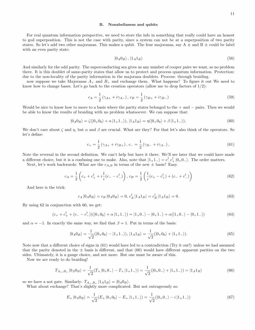
B. Nonabelianess and qubits

For real quantum information perspective, we need to store the info in something that really could have an honestto god superposition. This is not the case with parity, since a system can not be at a superposition of two paritystates. So let’s add two other majoranas. This makes a qubit. The four majoranas, say A ± and B ± could be labelwith an even parity state:

|0A0B� , |1A1B� (58)

And similarly for the odd parity. The superconducting sea gives us any number of cooper pairs we want, so no problemthere. It is this doublet of same-parity states that allow us to protect and process quantum information. Protection:due to the non-locality of the parity information in the majorana doublets. Process: through braiding.now suppose we take Majoranas A+ and B+ and exchange them. What happens? To figure it out We need to

know how to change bases. Let’s go back to the creation operators (allow me to drop factors of 1/2):

cA =1

2(γA+ + iγA−) , cB =

1

2(γB+ + iγB−) (59)

Would be nice to know how to move to a basis where the parity states belonged to the + and − pairs. Then we wouldbe able to know the results of braiding with no problem whatsoever. We can suppose that:

|0A0B� = ζ(|0+00�+ α |1+1−�), |1A1B� = η(|0+00�+ β |1+1−�), (60)

We don’t care about ζ and η, but α and β are crucial. What are they? For that let’s also think of the operators. Solet’s define:

c+ =1

2(γA+ + iγB+) , c− =

1

2(γB− + iγA−) , (61)

Note the reversal in the second definition. We can’t help but have it there. We’ll see later that we could have made

a different choice, but it is a confusing one to make. Also, note that |1+1−� = c†−c†+ |0+0−�. The order matters.

Next, let’s work backwards: What are the cA,B in terms of the new ± basis? Easy.

cA =1

2

�c+ + c†+ + i

1

i(c− − c†−)

�, cB =

1

2

�1

i(c+ − c†+) + (c− + c†−)

�(62)

And here is the trick:

cA |0A0B� = cB |0A0B� = 0, c†A |1A1B� = c†B |1A1B� = 0. (63)

By using 62 in conjunction with 60, we get:

(c+ + c†+ + (c− − c†−))(|0+00�+ α |1+1−�) = |1+0−� − |0+1−�+ α(|1+0−� − |0+1−�) (64)

and α = −1. In exactly the same way, we find that β = 1. Put in terms of the basis:

|0A0B� =1√2(|0+00� − |1+1−�), |1A1B� =

1√2(|0+00�+ |1+1−�). (65)

Note now that a different choice of signs in (61) would have led to a contradiction (Try it out!) unless we had assumedthat the parity denoted in the ± basis is different, and that (60) would have different apparent parities on the twosides. Ultimately, it is a gauge choice, and not more. But one must be aware of this.Now we are ready to do braiding!

TA+,B+|0A0B� =

1√2(T+ |0+0−� − T+ |1+1−�) =

1√2(|0+0−�+ |1+1−�) = |1A1B� (66)

so we have a not gate. Similarly: TA+,B+|1A1B� = |0A0B�.

What about exchange? That’s slightly more complicated. But not outrageously so:

E+ |0A0B� =1√2(E+ |0+00� − E+ |1+1−�) =

1√2(|0+0−� − i |1+1−�) (67)

12

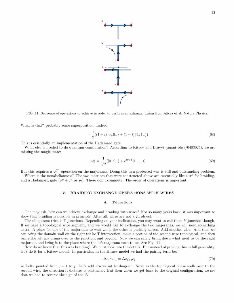
FIG. 11: Sequence of operations to achieve in order to perform an exhange. Taken from Alicea et al. Nature Physics.

What is that? probably some superposition. Indeed,

=1

2((1 + i) |0+0−�+ (1− i) |1+1−�) (68)

This is essentially an implementation of the Hadamard gate.What else is needed to do quantum computation? According to Kitaev and Bravyi (quant-phys/0403025), we are

missing the magic state:

|ψ� = 1√2(|0+0−�+ eiπ/4 |1+1−�) (69)

But this requires a√inoperation on the majoranas. Doing this in a protected way is still and outstanding problem.

Where is the nonabelianness? The two matrices that were constructed above are essentially like a σx for braiding,and a Hadamard gate (σy + σz or so). These don’t commute. The order of operations is important.

V. BRAIDING EXCHANGE OPERATIONS WITH WIRES

A. T-junctions

One may ask, how can we achieve exchange and braiding with wires? Not so many years back, it was important toshow that braiding is possible in principle. After all, wires are not a 2d object.The ubiquitous trick is T-junctions. Depending on your inclination, you may want to call them Y junction though.

If we have a topological wire segment, and we would like to exchange the two majoranas, we will need somethingextra. A place for one of the majornaas to wait while the other is pushing across. Add another wire. And then wecan bring the domain wall on the right tot he T intersection, make a portion of the second wire topological, and thenbring the left majorana over to the junction, and beyond. Now we can safely bring down what used to be the rightmajorana and bring it to the place where the left majorana used to be. See Fig. 11How do we know that this was braiding? We must look into the details. But instead of proving this in full generality,

let’s do it for a Kitaev model. In particular, in the Kitaev model we had the pairing term be:

−Δcjcj+1 = Δcj+1cj (70)

so Delta pointed from j + 1 to j. Let’s add arrows int he diagram. Now, as the topological phase spills over to thesecond wire, the direction it dictates is partiuclar. But then when we get back to the original configuration, we seethat we had to reverse the sign of the Δ.

13

If we hadn’t, we would run into a situation of Δ changing signs mid line. This leads to two degenerate Marjoanas,that can destroy the quantum information in the system.This is not the original configuration, is it? If we want to compare the braiding properly, we need to do a guage

transformation that will return the physics to what it was. To do it let’s invoke our knowledge of the BdG Hamiltonian,where Δ appears as:

Δτx (71)

So if Δ changed sign, and this became −Δτx, we need to do the following gauge transformation:

H → eiτz

2 πHe−i τz

2 π (72)

The transformation used is simple:

eiτz

2 π = cosπ

2+ iτz sin

π

2= iτz (73)

This transformation we can also apply to the MArjoanas. Recall from our calculation, that the left Majorana in aKitaev wire has the form:

γL =1

i

�1−1

�, γR =

�11

�(74)

These majoranas replace lable by the T-junction manipulation, which ends up with a Δ → −Δ. But the gauge trans-formation will fix that. Now comes the moment of truth! What do we get at the end, after the gauge transformationback?

γR → UγR = iτz�

11

�= −γL (75)

and:

γL → UγL = τz�

1−1

�= γR (76)

Just as with Ivanov. So this works.

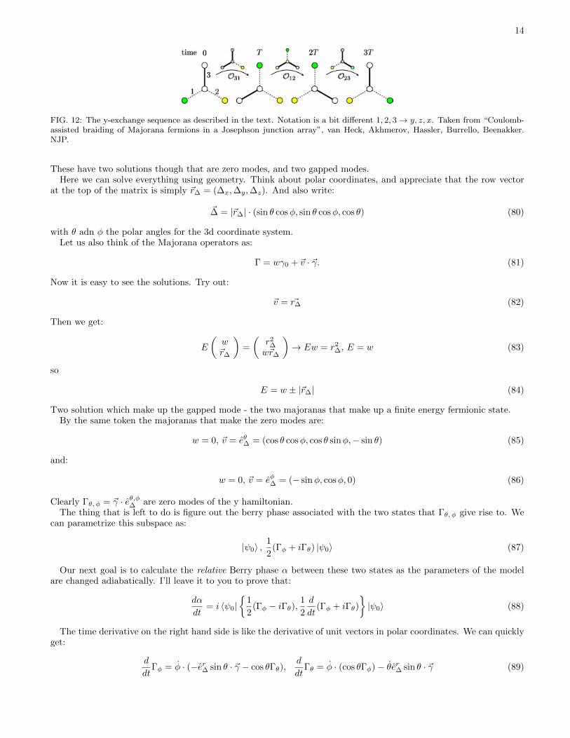
B. The y-setup for braiding

From a practical perspective, it might be best to have a stationary configuration where we only change fluxes. Sucha configuration was suggested by Beenakker’s group. By putting together three wires, all in the topological phase, weachieve a hamiltonian of coupling that is:

H = −iΔxγ0γx − iΔyγ0γy − iΔzγ0γz (77)

For reasons I will not explain now, but you are welcome to read Beenakker’s paper ... the couplings Δα wereexponentially controlled by a flux that controlled the proximity of the wire to a superconductor. Roughly:

Δα ∼ e−c√

| cosΦα| (78)

This allowed tuning each of hte arms between zero coupling and a coupling much bigger than the others with greatease, even if precision of the flux control is lacking.This is a cool setup for exchange. If we start with Δx = 1,Δy = Δz = 0, then we have two zero modes clearly

lodged at the y and z sides of the y. Now doing clock moves, and making Δy → 1, Δx → 0, will shift γy → γx. Thendoing Δy → 0, Δz → 1, shifts γz → γy. Lastly, Δz → 0, Δx → 1, shifts γz → γy, brings what used to be γy to γz.That’s it - we facilitated an exchange. See Fig. 12When engaging with such an hamiltonian, all we want, really, is to find ladder operators of the form Γ = xγx +

yγy + zγz + wγ0 Commuting Γ with H, seeking [H,Γ] = �Γ, we find that this maps to the Schrodinger equation:

E

wxyz

= i

0 −Δx −Δy −Δz

Δx 0 0 0Δy 0 0 0Δz 0 0 0

wxyz

(79)

14

FIG. 12: The y-exchange sequence as described in the text. Notation is a bit different 1, 2, 3 → y, z, x. Taken from “Coulomb-assisted braiding of Majorana fermions in a Josephson junction array”, van Heck, Akhmerov, Hassler, Burrello, Beenakker.NJP.

These have two solutions though that are zero modes, and two gapped modes.Here we can solve everything using geometry. Think about polar coordinates, and appreciate that the row vector

at the top of the matrix is simply �rΔ = (Δx,Δy,Δz). And also write:

�Δ = |�rΔ| · (sin θ cosφ, sin θ cosφ, cos θ) (80)

with θ adn φ the polar angles for the 3d coordinate system.Let us also think of the Majorana operators as:

Γ = wγ0 + �v · �γ. (81)

Now it is easy to see the solutions. Try out:

�v = �rΔ (82)

Then we get:

E

�w�rΔ

�=

�r2Δw�rΔ

�→ Ew = r2Δ, E = w (83)

so

E = w ± |�rΔ| (84)

Two solution which make up the gapped mode - the two majoranas that make up a finite energy fermionic state.By the same token the majoranas that make the zero modes are:

w = 0, �v = eθΔ = (cos θ cosφ, cos θ sinφ,− sin θ) (85)

and:

w = 0, �v = eφΔ = (− sinφ, cosφ, 0) (86)

Clearly Γθ,φ = �γ · eθ,φΔ are zero modes of the y hamiltonian.The thing that is left to do is figure out the berry phase associated with the two states that Γθ,φ give rise to. We

can parametrize this subspace as:

|ψ0� ,1

2(Γφ + iΓθ) |ψ0� (87)

Our next goal is to calculate the relative Berry phase α between these two states as the parameters of the modelare changed adiabatically. I’ll leave it to you to prove that:

dα

dt= i �ψ0|

�1

2(Γφ − iΓθ),

1

2

d

dt(Γφ + iΓθ)

�|ψ0� (88)

The time derivative on the right hand side is like the derivative of unit vectors in polar coordinates. We can quicklyget:

d

dtΓφ = φ · (−erΔ sin θ · �γ − cos θΓθ),

d

dtΓθ = φ · (cos θΓφ)− θerΔ sin θ · �γ (89)

15

From that we see that:

�(Γφ − iΓθ),

ddt (Γφ + iΓθ)

�=

�(Γφ − iΓθ),−Γθφ cos θ + iφ · cos θΓφ

�

= 2iφ cos θ.(90)

And finally, we get:

dα

dt= −φ cos θ (91)

just like a spin-1/2. up to a missing factor of a half.Doing the clock moves from above, then, cover an octant - so an eighth - of the sphere, and the phase associated

with that is:

αexchange =1

42π =

1

2π, eiαexchange = i (92)

As expected.Why am I teaching you this? It is a neat example of how Majorana fermions will be manipulated in practice, it is

also the key for making the Kitaev-Bravyi magic states, I believe. But for that, stay tuned!