arX

iv:1

607.

0594

9v4

[ph

ysic

s.ge

n-ph

] 1

8 Ju

n 20

18

Main Physical Aspects of the Mathematical Conception

of Energy in Thermodynamics

V. P. Maslov

National Research University Higher School of Economics, Moscow, 123458, Russia;Department of Physics, Lomonosov Moscow State University, Moscow, 119234, Russia;

Ishlinsky Institute for Problems in Mechanics,Russian Academy of Sciences, Moscow, 119526, Russia;

v.p.maslov@mail.ru

Abstract

We consider the main physical notions and phenomena described by the author inhis mathematical theory of thermodynamics. The new mathematical model yields theequation of state for a wide class of classical gases consisting of non-polar moleculesprovided that the spinodal, the critical isochore and the second virial coefficient aregiven. As an example, the spinodal, the critical isochore and the second virial coefficientare taken from the Van-der-Waals model. For this specific example, the isothermsconstructed on the basis of the author’s model are compared to the Van-der-Waalsisotherms, obtained from completely different considerations.

Keywords: Van-der-Waals model; compressibility factor; spinodal; number of de-grees of freedom; admissible size of clusters; quasi-statical process.

1 Introduction

In the present paper, we present the foundations of the new mathematical model of thermo-dynamics for the values of the energy for which the molecules are in the pre-plasma state,in particular as pressure P is near-zero.

The new mathematical model constructed by the author in the cycle of papers [1]–[2],differs somewhat from the commonly accepted model of phenomenological thermodynamicsand allows us to construct the equation of state for a wider class of classical gases.

We mainly study the metastable states in the case of gases and in the case of fluids upto the critical isochore ρ = ρc. The liquid isotherms are divided into two parts: the regionwith temperatures near the critical temperature Tc and the region of the “hard” liquid whoseisotherms pass through the point of zero pressure.

Further, the distributions in the Van-der-Waals model are compared to the distributionsappearing in the author’s new model for classical gases with given critical temperatures, inparticular, with Van-der-Waals critical temperature. The precision with which the isothermsconstructed from the author’s theory coincide with the Van-der-Waals isotherms turns outto be less than the accepted precision in experimental studies. The probability of such acoincidence being accidental is “infinitely small”.

All the distributions of energy levels for classical gas considered in the present paperhave been established mathematically, see [1]–[3] and references therein) and have met withapproval (see, for example, the review [4], published in the journal “Probability Theory and

1

its Applications” in connection with the State Prize of the Russian Federation in Scienceand Technology granted to the author in 2013 (for developing the mathematical foundationsof modern thermodynamics).

2 Van-der-Waals Normalization and the Law of

Corresponding States

The correct choice of units of measurement for different gases allowed Van-der-Waals tocompare the parameters of the gases to dimensionless quantities, thus obtaining the famous“law of corresponding states”.

For every gas, there exists a critical temperature Tc and a critical pressure Pc such thatif the temperature or the pressure is greater than their critical values, then gas and liquidcan no longer be distinguished. This state of matter is known as a fluid.

The Van-der-Waals “normalization” consists in taking the ratio of the parameters bytheir critical value, so that we consider the reduced temperature Tr = T/Tc and the reducedpressurePr = P/Pc. In these coordinates, the diagrams of the state of various gases resembleeach other – this a manifestation of the law of corresponding states.

The equation of state for the Van-der-Waals gas in dimensionless variables has the form:

(Pr + αρ2)(1− αρ) = ρTr, (1)

where α = 33/26, α = 1/23, and the dimensionless concentration (density) ρ = N/V ischosen so that ρc = 8/3 in the critical point.

In thermodynamics, the dimension of the internal energy E is equal to the dimension ofthe product PV of the pressure by the volume. On the other hand, temperature plays therole of mean energy E/N of the gas (or of the liquid). For that reason, when the dimension oftemperature is given in energy units, the parameter Z = P/ρT , known as the compressibility

factor, is dimensionless. For the equation of state of the gas or liquid, the most naturaldiagram is the Pr-Z diagram, in which the dimensionless pressure Pr is plotted along thex-axis and the dimensionless parameter Z, along the y-axis. A diagram with axes Pr, Zis called a Hougen–Watson diagram. In the Van-der-Waals model, the critical value of thecompressibility factor is

Zc =PcVc

NTc

=3

8.

In Figs. 2–1, the Van-der-Waals isotherms are shown in a Pr-Z Hougen–Watson dia-gram, for which we used the normalization Pr = P/Pc, Tr = T/Tc, where Tc is the criticaltemperature.

3 On the Number of Degrees of Freedom and the Par-

tition Theory of Integers

In the physics literature, the notion of number of degrees of freedom is used for ideal gases,in which particles do not interact. In probability, the number of degrees of freedom is alsoconsidered independently of any interaction.

When physicists speak of the number of degrees of freedom, they usually have in mindthe number of degrees of freedom of a single molecule. Normally, a one-atom molecule willhave 3 degrees of freedom, a two-atom molecule, 5. In a gas, the molecules move with

2

Figure 1: Van-der-Waals isotherms on the Pr-Z diagram. On the plot P = Pr, T = Tr.The curve shown by the fat hashed line is the critical isotherm Tr = 1. The dotted line isthe spinodal, the thin hashed line is the binodal.

.

Figure 2: The Pr-Z diagram for the Van-der-Waals equation with P = Pr.

different speeds and different energies; although their mean energy – temperature – is thesame, their individual energies may be different, and the number of degrees of freedom ofdifferent molecules can also differ. Thus a two-atom molecule with very high energy mayhave a number of degrees of freedom greater than than 5, and this will affect the mean value(average over all molecules) of the number of degrees of freedom of the given gas. This meanvalue is called the collective number of degrees of freedom of the gas, and is a fractional ratherthan a whole number.

A one-atom molecule has 3 degrees of freedom, a two-atom molecule, 5. Two-atommolecules are regarded in [5] as molecules of ideal gas. Nevertheless, saying that the numberof degrees of freedom of a molecule is 5 means that we are implementing an exclusion rule:we are saying that one of the degrees of freedom is excluded. More precisely, we regard themolecule as a dumbbell, and exclude its oscillations as a rod. However, if the temperatureincreases, these “rod” oscillations will take place and so, for sufficiently high temperatures(energies), the molecules will have a greater fractional number of degrees of freedom.

In the author’s model, the number of degrees of freedom is an important independentparameter, so that the notion of exclusion need not be defined by means of some internal

3

considerations 1.Although the collective number of degrees of freedom of a classical gas can be deter-

mined by the initial interaction between its particles, in the probabilistic description of thegeneralized ideal gas (a notion that we present in Section 5), this parameter is introducedindependently.

If nuclear forces are taken into consideration, it can be shown that a wide class of two-atom molecules have 5 degrees of freedom, but this is difficult to establish. And so we preferto stipulate axiomatically, as in probability theory, that on a given energy level there can beonly one or, say, no more than K particles.

Another important consideration is that we do not take into account the number ofparticles and the volume separately, we consider their ratio – density (concentration).

The consideration of density alone leads to the following important consequence in ther-modynamics: density does not depend on the numeration of particles contained in the givenvolume. Whatever the numeration of the particles, the density remains the same. It iscommonly believed (in particular, it is stated in the book [7]) that classical particles differfrom quantum particles in that they can be numbered and then the motion of any individualparticle can be followed by keeping track of its number. This is correct, but if the behaviorof a multi-particle system is described by equations involving density, e.g. via a probabilitydistribution, then such a description does not depend on the numbering of particles.

Therefore, all the results from quantum mechanics that follow from the remarkable factthat the solution does not depend on numeration can be carried over to the description ofany classical multi-particle system by means of equations containing density2.

As an illustrative example, we consider the purchase of 1 kilogram of granulated sugar.If this amount of sugar is measured by calculated the grains (and thus the grains must befirst numerated), then it is obvious that this process takes a lot of time. Assume that thebuyer has a fixed time for the measurement tmes which is equal to one hour and there is nobalance to weight the sugar. Then the buyer will measure the granulated sugar by usingsome vessels. The results of weighting and of measuring by vessels does not change if twograins in the measured volume interchange their places. This means that (1) the particle

identity principle holds for the sugar grains and (2) the sum of particles is independent of

their location, i.e., the arithmetic property is satisfied [9]. In particular, this implies thatone can use a Bose–Einstein-type distribution in this “classical” situation.

The exclusions that we impose will lead us to a more general distribution in which westipulate that no more than K particles are on the same energy level. The natural numberK will be called the maximal occupation number or maximal admissible size of clusters.

The corresponding energy distribution, often called parastatistical [10]–[11], will be de-scribed in the next sections. To specific and generalize the parastatistical distributions, weshall use the above-listed items (1) and (2).

1Sometimes, instead of the number of degrees of freedom, such notions as free will or freedom of choiceand so on are considered (see, e.g. [6]).

2In particular, the most important thing in the chapter on identical particles in [7] is the method ofsecondary quantization introduced by Dirac and neatly explained in mathematical terms by Fock (the Fockspace, the creation and annihilation operators and so on). Since density does not depend on numeration,the method of secondary quantization had been carried over to classical multi-particle systems described byequations depending on density. This was done by Schoenberg in 1953–54. Later Schoenberg’s approachwas generalized in the author’s joint article with O.Yu. Shvedov [8].

4

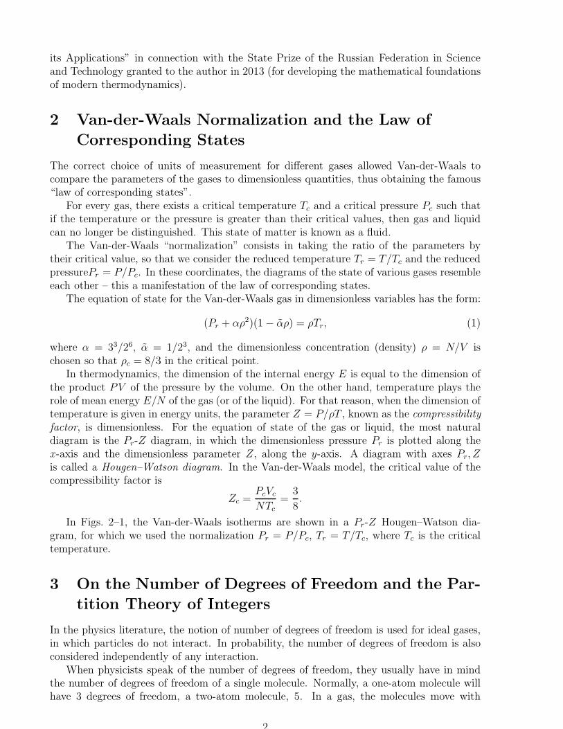
Remark 1. In the Landau–Lifshits textbook [5], two relations are given as the basic equations

∑

j

Nj = N, (2)

∑

j

εjNj = M,

where M is the energy, N is the number of particles and εj is a discrete family of energylevels (see [12], [13]).

The values εj in Eq. (2) are related to the existing interaction potential for the particles.It turns out that if we use the interaction with collective number of degrees of freedom equalto D, then we must put3

εj = const · jD/2, (3)

i.e.,

M =∑

j

const · jD/2Nj . (4)

This statement is a theorem proved in the author’s paper [14].

The first person who noticed the unexpected relationship between the partition problemin number theory (in particular the famous discovery of Ramanujan) and nuclear disintegra-tion, was Niels Bohr, the founder of quantum theory (see [15]).

It is well known that Bohr’s most famous opponent was the great Albert Einstein himself.The polemic between Bohr and Einstein, during which Bohr gave convincing answers to allof Einstein’s counterarguments, only fortified Bohr’s position and helped him in developinghis quantum approach. In a commentary to one of Einstein’s letters, Max Born wrote: “...Einstein’s attitude to quantum mechanics was a heavy blow to me, he refuted the theorywithout any argumentation, only referring to his ‘inner voice’...” [16]. It was only afterthe experimental corroboration of the disintegration of heavy Lithium [17] and Uranium-235that Einstein did support, albeit reluctantly, the A-bomb project.

The Bohr–Kalckar paper [18] of 1937 was the first work in which the coincidence of“thermodynamical formulas” with the number-theoretic formulas for partitions of integersinto sums was discovered. Here is a quotation from that paper. “Under the simplifyingassumption that each level is the combination of a certain number of quantities assumingnearly equidistant values, one can easily calculate the density of nuclear levels under highperturbations. Denote by p(M) the number of possible ways of presenting a positive integeras a sum of smaller positive integers. An asymptotic formula for p(M) was obtained byG. Hardy and S. Ramanujan. For large values of M this formula may be approximatelywritten in the form

p(M) ∼ 1

4√3M

eπ√

2

3M .

Let us choose 2·105eV for the unit of energy, which approximately corresponds to the commondistance between the lowest levels of the heavier nuclei. For the number of partitions forwhich the perturbation energy of 8 ·106eV will be obtained, we will then find p(M) ∼ 2 ·104.This means that the mean distance between levels approximately equals 10eV , which roughlycorresponds to the densities of distribution of levels calculated from the collisions of slowneutrons. 〈. . . 〉 The formulas for the density of nuclear levels obtained by analogy withthermodynamics practically coincide, at least in the exponential dependence on the total

3The Landau–Lifshits book gives a more general system of equations, later specified in [22], [23]:∑

j εjNj = E, εj = j2/D. For Landau M = E is energy.

5

energy of excited nuclei, with the formula for p(M) if one understands the number M asthe measure of total energy expressed as the difference of energies between the lowest levelstaken for the unit of measure” (see pp. 337–338 in the Russian translation [18]).

Bohr’s and Kalckar’s considerations about the distance between lowest energy levelsis correct, because for the Schrodinger equation, the equations of the lower levels in thepotential trough are quadratic.

Note that the probability of the coincidences indicated by Bohr and Kalckar being acci-dental is practically zero.

Later Bohr proposed using Uranium-235 as an example of the nucleus of an atom, sinceit was most appropriate for his construction and used it to explain how to generate a nuclearreaction [19].

The historian and archivist of the British Committee for Atomic Energy Margaret Going,on the basis of her study of the opinions of authoritative physicists, wrote: “... The workof English and American scientists on the A-bomb came directly from articles of ProfessorBohr and Doctor Wheeler...”. Thus we may conclude that the creation of the A-bomb wasbased on the fantastic discovery of Ramanujan.

An essential role in establishing the new world outlook in physics was played by thenumerous volumes of the famous treatise by Landau and Lifshits, in particular, [5] and [20].In the book [5] in Section 40 “Nonequilibrium ideal gas,” the authors present the system ofequations (2) and (3)–(4), on which their further exposition is based. Both N and Nj in theseequations are integers. And so equations (2) coincide with the Diophantine equations forpartitions in number theory. In the subsequent sections of the book [5] the main equationsof thermodynamics are obtained without appealing to the so-called three main principles of

thermodynamics, which appear in all textbooks on thermodynamics, but not in [5].Bohr’s paper [18] generated only a trickle of mathematical and physical papers, in which

the connection between the statistics of Bose–Einstein and Fermi–Dirac and the Ramanujanformula was studied in more detail [22]–[24]. Thus papers on this topic appeared in themathematical journal “Mathematical Proceedings of the Cambridge Philosophical Society.”It was shown that if one takes into account the connections with partition theory, the Ra-manujan formula and the Hardy–Ramanujan theorem in number theory, then it becomesclear that, in the case when there are repeated summands in the partition, the leading termof the Ramanujan formula coincides with the entropy of the Bose–Einstein statistics, whereasin the case when there are no repeated summands, this term coincides with the Fermi–Diracentropy (bosons and fermions – no other particles are observed). Apparently, one of the lastpapers in this series is [24]. It contains a bibliography of the topic. But overall it seems thatcontemporary physicists did not pay attention to that series of papers and forgot that theyare indebted to Ramanujan for the remarkable revolution in the scientific world outlook.

It follows from Bohr’s paper that his model of the nucleus of an atom does not involvethe interaction of particles in the form of attraction. When Bohr visited the USSR in 1961,he demonstrated a simple model of a nucleus consisting of little balls in a cup. Several ballswere placed in a cup, and then another little ball, endowed with a certain energy, was slippedinto the cup. Were the cup empty, the new ball would have slipped out of the cup, but itshared some of its energy with the other balls and stayed in the cup. This is due to thefact that all the balls were in a common potential field. Thus Bohr regarded the nucleus asconsisting of particles that do not attract each other.

Bohr’s model of the nucleus is a model without attraction of molecules, and so is Frenkel’smodel of liquid (liquid drop model). Such a model of the nucleus appears to contradict thephysical viewpoint as well as the commonsense (or naive) point of view. Nevertheless, itadequately describes nuclear fission, and Frenkel’s model adequately describes the behavior

6

of liquids. The Frenkel model contains “holes” but does not involve mutual attraction ofmolecules.

Incidentally, Frenkel subtly complained about the difficulties of overcoming traditionalviewpoints, using the word “we,” i.e. “physicists.” He writes: “We easily get used to uniformand steady things, we stop noticing them. What is habitual seems understandable, but wedon’t understand the new and unusual, it seems unnatural and obscure 〈. . . 〉. Essentially,we never really understand, we can only get used to” [25, p. 63]. If we follow Bohr, we seethat in the thermodynamics that he talks about (see above), there is no attraction betweenmolecules, but there is a common potential, in particular the Earth’s gravitational attraction.Molecules can collide, as they do in ideal gas, but there is no mutual attraction.

In Bohr’s paper mentioned above, he noted the connection between nuclear fission andthe theory of partitions in number theory. On the other hand, he proposed the drop liquidmodel of the nucleus. This leads us to the idea that the theory liquids is also connectedto partition theory. In that connection Bohr writes only about the analogy with thermo-dynamics, and so, like his pupil Landau, this means that they did not have in mind theold thermodynamics based on the “three fundamental principles,” but the thermodynamicsunderstood in the framework of the new world outlook based on Bohr’s quantum theorypostulates and partition theory.

The author, following the way traced out by Bohr and Landau, has developed a math-ematical approach based on number theory problems and quantum theory. In the author’smodel there is no attraction between particles4, but there is a common potential, in partic-ular, the potential due to the Earth’s gravitation and its rotation.

The author has shown that his approach to thermodynamics yields the same formulasas partition theory with logarithmic precision (which means the formulas coincide from thepoint of view of tropical arithmetic). The notion of logarithmic accuracy was introduced inVol. X of the Landau–Lifshits textbooks [20] on p. 211. It is defined as follows: logarithmicaccuracy of M means that we find M not up to o(M), but only up to o(ln(M).

Before passing to the formulation of the main formulas and results, we recall the notionsof tropical arithmetic and logarithmic accuracy.

The arithmetics of a system may be decimal or binary. The well-known notion of integerpart of a real number, entier, is denoted by square brackets: [a] stands for the maximuminteger that does not exceed a given real number a. It is this integer that is usually retainedin human memory. For example, although the number 2.99 is close to 3, our memory retainsits integer part 2; this peculiarity is used by marketing people when assigning prices tocommodities in shops.

From the viewpoint of arithmetics, it is quite natural to discard the fractional part forsufficiently large a. If the numbers are as large as is common for macroscopic systems, itis convenient to use a generalization of this notion for large numbers. By [a]10 we denotedecimal arithmetics, where [·]10 means the same entier for rationals but with respect to 10.For example, [15]10 = 10, [90]10 = 10, [105]10 = 100, and [6 · 1023]10 = 1023.

For the sum, we have [1015 +1014]10 = 1015; i.e., the sum equals max(1015, 1014). For theproduct, 1015 · 1014 = 1029; i.e., the product is equal to the number of zeros in a multidigitnumber.

Similar rules hold for a system considered in the binary arithmetics [a]2.The arithmetics thus constructed not only corresponds to the (max,+)-algebra but also

takes into account precision and neglects c-numbers, just as it happens in the Maslov–

4To be more precise, attraction between particles is used only at the boundary conditions in fixing theexperimental values of the first and second virial coefficient of the given gas. Also note that thermodynamicsis constructed with “logarithmic accuracy.”

7

Litvinov dequantization. Hence we can say that this arithmetics is “tropical.”For the natural logarithm, we deal with a special situation. Here we must use the great

formula due to the great Ramanujan and the natural logarithm of the solution given by thisformula. By considering the integer parts [loge p(M)], we obtain a partition of p(M) intosimilar subsets of integers.

Note that the use of the natural logarithm is natural if the formulas use the polyloga-rithm, because the polylogarithm emerges from the Stirling formula, and the Stirling formulacontains Euler’s number e.

Thus, in addition to the arithmetics described by the entiers [·]10 and [·]2, we introducethe arithmetics [·]e on the basis of partition theory.

Definition 1. We say that two numbers coincide with logarithmic accuracy if the valuesof their normal arithmetics [·]e coincide. In other words, lnA ∼= lnB means that lnA =lnB + o(lnB).

Since this arithmetics puts all elements coinciding with each other with “logarithmicaccuracy” into the same equivalence class, we see that convergent series are equivalent topolynomials. It follows that, to each series Φ, we can assign the degree of the correspondingpolynomial. We denote this number by n(Φ). If one can assign an enveloping series to adivergent series, then the minimum number of the enveloping series naturally determines thedegree n(Φ) of the corresponding polynomial.

Now we can briefly present a classical problem in partition theory of integers renewed bythe inclusion of the number zero and negative entropy (negentropy).

First, consider some examples.

Example 1. If we partition the number 5 into 2 summands, zero summands not allowed, thenwe obtain pN(M) = 2, 5=4+1=3+2, where N is the number of summands, N = 1, 2, . . . ,M ,and pN(M) is the number of partitions of M into N summands. There are two possiblepartitions in this example for N = 2.

Example 2. Let us allow zero summands in partitions ofM into N summands. Then pN(5) =3 for N = 2 in the preceding example, 5=5+0=4+1=3+2. All in all, there are three possiblepartitions in this case.

When partitioning 5 into 3 with zeros allowed, the pN(M) partitions without zeros,5 = 3 + 1 + 1 = 2 + 2 + 1 = . . . , are supplemented with partitions containing zeros,4 + 1 + 0 = 3 + 2 + 0 = 5 + 0 + 0. With zeros taken into account, all preceding partitionsare repeated; i.e., we obtain the sum of all partitions without zeros.

We introduce the following notation:ps(M) =

∑si=1 pi(M).

Proposition 1. The number of partitions of M into N summands, zero summands allowed,

coincides with ps(M) for s = N .

Definition 2. Let qN (M) be the number of partitions of M into N distinct summands, andlet

q(M) =∑

N

qN(M).

By definition, the partition 3+1+1 of 5 into 3 terms is excluded from qN(M). All thezeros are excluded as well.

Let us continue the partition pN(M) by the numbers qN(M). This continuation is con-tinuous, because for M = 1 there are two partitions, M = 1 = 1 + 0, taken into account inpN (M) and one partition, qN(1) = 1, taken into account in qN (M).

8

We define natural entropy as the natural logarithm of pN (M) and natural negentropy asthe natural logarithm of qN(M). The passage through the point M = 1 is the passage frompositive natural entropy into negative natural negentropy loge(qN(M)).

Since p1(M) = 1 and pM(M) = 1, it follows that there exist maxima between N = 1 andN = M . Of these maxima, take the maximum value N .

Since pN (M) decreases for N > N and pN(M) is nondecreasing, we see that the increasein pN(M) can only be due to the increase in the number of zeros.

4 The Equation of State

In the simplest version of thermodynamics, one considers the conjugate extensive-intensivepairs pressure-volume, temperature-entropy, chemical potential-number of particles.

One of the main notions of thermodynamics is the equation of state. In 6-dimensionalphase space, where the intensive thermodynamical variables P , T , and −µ play the roleof coordinates and the corresponding extensive variables V , −S, and N play the role ofmomenta, the equation of state is described by a 3-dimensional surface on which severaladditional identities, corresponding to the so-called thermodynamical potentials, hold. Thisresults in the fact that this 3-dimensional surface is a Lagrangian manifold5, and the ther-modynamical potential corresponds to action in mechanics.

If one does not consider the number of particles and the volume separately, and onlyconsiders their ratio, i.e., density, then one variable turns out to be redundant, and we canconsider 4-dimensional phase space and the 2-dimensional Lagrangian surface.

If the volume V is given, we can use a single thermodynamical potential Ω that can beexpressed as follows:

dΩ = (−S) dT +N d(−µ), Ω = −PV. (5)

Besides, since the internal energy is M = const ·PV , it is customary in thermodynamicaldiagrams to plot the pressure P along the abscissa axis, as this was done in the Hougen–Watson diagram.

On the Pr-Z diagram, the spinodal is defined as the curve which is the locus of all pointswhere the tangents to the isotherms are perpendicular to the Pr axis (see Figures 2 and 1).

The mathematical model constructed by the author in the papers [1]–[2], which uses thedensity “effect” mentioned in Section 3 above, shows that

1) if the spinodal in the gaseous region for any gas with non-polarized molecules is given,then all the gas isotherms can be constructed;

2) if we know the slope of the isotherm for Pr = 0 on the Pr-Z diagram (this is equivalentto knowing the value of the second virial coefficient [36]) as well as the critical isochore forany fluid (the supercritical state for any collection of non-polarized molecules), then we canconstruct all the isotherms of the fluid up to the critical isochore;

3) if we know the liquid binodal for any gas consisting of non-polarized molecules, andalso know the pressure Pr and the density ρ on the line Z = 1 (the Zeno line), then we canconstruct the liquid isotherms passing through the point Pr = 0, Z = 0 for so called “hard”liquid consisting of non-polarized molecules on the interval 0 ≤ Z ≤ 1.

5In the data base MathSciNet (American Mathematical Society) the query to MathJax on Publicationsresults for “Anywhere =(Maslov index) OR Anywhere (Maslov class)” in a list of 575 papers published before2013, where the notions “Lagrangian submanifolds” [29], “Maslov index”, “Maslov class” are developed andextended. See also [30]–[31] and so on.

9

For an arbitrary liquid, by the Temperley temperature we mean the minimal temperatureof the set of liquid isotherms passing through the point Pr = 0, Z = 0. This temperature(corresponding to K = ∞ ), calculated by the physicist Temperley for the Van-der-Waalsgas, equals 33/25Tc [35].

As proved by the author in [1]–[2], the corresponding distribution can be expressed interms of the polylogarithm6

Lis(z) =∞∑

k=1

zk

ks= z +

z2

2s+

z3

3s+ . . . (6)

This distribution yields the following expressions for the thermodynamical potential Ω, thedensity (concentration) ρ and the reduced pressure Pr:

Ω = −Λ(γ,K)T 2+γr

Li2+γ(a)−1

(K + 1)1+γLi2+γ(a

K+1)

, γ = γ(Tr). (7)

ρ(Tr, γ,K) =Λ(γ,K)

ζ(2 + γc)T 1+γr

(

Li1+γ(a)−1

(K + 1)γLi1+γ(a

K+1)

)

, (8)

Pr(Tr, γ,K) =Λ(γ,K)

ζ(2 + γc)T 2+γr

(

Li2+γ(a)−1

(K + 1)1+γLi2+γ(a

K+1)

)

, (9)

where K is the maximal occupation number, a = eµ/Tr (a is called the activity), γ = D/2−1,D is the collective number of degrees of freedom, Λ(γ,K) is a normalizing constant.

For each type of gas, the critical parameters Tc, Pc, ρc are determined experimentally.Substituting these values into (8)–(9), we can determine the parameters γ = γc and K = Kc.The parameter γc is the number of collective degrees of freedom Dc = 2γc + 2 of the criticalisotherm. By Kc we denote the admissible size of clusters (maximal occupation number)7

at the energy level of the critical point.Using (7) and the fact that

M = −µ(∂Ω)/(∂µ) − T (∂Ω)/(∂T ) + Ω,

where Ω = −PV , we derive M = (D/2)PV .

5 Entropy and Negentropy

Above we introduced the notionLet l be the number of particles on a given energy level. If we impose the restriction

that each energy level can host at most K particles, l ≤ K, then we arrive at the Gentilestatistics, also known as parastatistics, and we have the following relation, which generalizesthe Bose–Einstein statistics as K → ∞ and the Fermi–Dirac statistics for K = 1:

N =Λ

Γ(γ + 1)

∫ ∞

0

(

1

(eξ/T−µ/T − 1)− K + 1

(e(K+1)(ξ/T−µ/T ) − 1)

)

ξγ dξ, (10)

M =Λ

Γ(γ + 2)

∫ ∞

0

(

1

(eξ/T−µ/T − 1)− K + 1

(e(K+1)(ξ/T−µ/T ) − 1)

)

ξγ+1 dξ, (11)

6Note that for z = 1 and Re(s) > 1, Lis(1) = ζ(1) is Riemann’s zeta function.7The separation of the clusters of molecules near the flat surface of a liquid for T = Tc can be observed

experimentally.

10

where where T is the temperature, γ = D/2 − 1, and Λ is the parameter to be determinedin number theory. In quantum mechanics, it depends in a well-known way on the mass andthe Planck constant [15].

Indeed, if K = 1, then (without restrictions on the value of the chemical potential µ) weobtain the Fermi distribution

N |K=1 =Λ

Γ(γ + 1)

∫ ∞

0

1

exp(ξ − µ)/T+ 1ξγ dξ. (12)

For K = ∞, the formula coincides with the usual Bose–Einstein distribution. For µ = 0and γ = 0 the solution has a singularity; it becomes infinite.

To regularize the integral (10) for K = ∞, since l ≤ N , we apply formula (10) withK = N . From (10), we obtain the relation

N = Λ

∫ ∞

0

(

1

expε/T − 1− N + 1

exp(N + 1)ε/T − 1

)

dε. (13)

Since the relations

N = −ΛT log(1− a), M = ΛT 2 dilog(1− a), (14)

where dilog(1 − a) = Li2(a), hold for the Bose–Einstein distribution with a < 1 in thetwo-dimensional case, we start by finding Λ.

Since the Ramanujan formula for pM(M) gives the first term of the expansion as M → ∞in the form

loge pM(M) ∼= 2√

Mdilog(0) , (15)

and the first term of the expansion of the entropy is of the form (see [22, formula 20])

S ∼= 2Λ√

Mdilog(0) , (16)

we see that Λ ≡ 1.Let N = Nc be the solution of Eq. (13). Consider the value of the integral in (13) (with

the same integrand) taken from δ to ∞ and then pass to the limit as δ → 0. After makingthe change βx = ξ in the first term and β(Nc +1)x = ξ in the second term, where β = 1/T ,we obtain

Nc =1

β

∫ ∞

δβ

dξ

eξ − 1−∫ ∞

δβ(Nc+1)

dξ

eξ − 1+O(δ) =

1

β

∫ δβ(Nc+1)

δβ

dξ

eξ − 1+O(δ) (17)

∼ 1

β

∫ δβ(Nc+1)

δβ

dξ

ξ+O(δ) =

1

βln(δβ(Nc + 1))− ln(δβ)+O(δ) =

1

βln(Nc + 1) +O(δ).

(18)

On the other hand, after neglecting the second summand in the integrand of (11) for largeM and making the change βx = ξ, we can write

1

β2

∫ ∞

0

ξ dξ

eξ − 1∼= M. (19)

After passing to the limit as δ → 0 and expressing β, from (19), we obtain

Nc =

√

M

dilog(0)log(Nc + 1). (20)

11

The ideal entropy is the same for the Fermi and Bose particles (see [22, Eq. (13a) as wellas Eqs. (20) and (27)]).

Hardy and Ramanujan derived the formula

p(M) =1

(4√3)M

eπ√

2M3 . (21)

The asymptotic formula for q(M) has the form [26]

q(M) =1

(4 · 31/4)M3/4eπ√

M/3. (22)

If a fermion nucleus emits a single neutron, it becomes a boson, and vice versa. Thus,the energy density flattens out under the successive emission of neutrons according to Bohr’sconcept [18].

By (21) and (22), boson fission overtakes fermion fission as M → ∞. For a boson notto become a fermion when emitting neutrons, it must emit them in pairs, which may bringabout fission of the nucleus. For the Bose–Einstein distribution (20), the critical value of Nc

satisfies the implicit relation

Nc =

√

M

ζ(2)ln(Nc + 1). (23)

Therefore,

M = ζ(2)

(

Nc

lnNc

)2

. (24)

As we see, this value corresponds to the limit value of activity a = 1 (i.e., the chemicalpotential µ = 0). In this case, we use the Gentile statistics to obtain self-consistent equations.Similarly, for the Fermi system, this limit values corresponds to a → −∞ so that

M =Nc(Nc − 1)

2+ ζ(2)

(

Nc

lnNc

)2

. (25)

These relations can be derived using the Bose and Fermi statistics and the Gentile statistics.By the Bohr–Kalckar “correspondence principle” between the physical notion of nucleus

and number theory, we can transfer these relations to the above-cited construction of numbertheory with the zeros taken into account [15], [27]. We have

p

(

ζ(2)

(

Nc

lnNc

)2)

= q

(

Nc(Nc − 1)

2+ ζ(2)

(

Nc

lnNc

)2)

. (26)

This formula allows us to determine the point Nc such that, for N > Nc, the entropy ofthe branch with repeated terms and zeros becomes greater than the entropy of the branchwithout repetitions and zeros.

The mesoscopic values in number theory correspond to dimension (number of degrees offreedom) equal to 2, i.e. in the region, where the parameter k varies from 0 to 90, Let usfind these values Nc from the relation

M = T 2ζ(2)

(

1− 1

(Nc + 1)

)

, (27)

where T can be found from the relation [28]

Nc = T ln(Nc + 1). (28)

12

Figure 3: The dependence of the entropy S on N for M = 70. The upper curve is obtainedwhen zero summands are allowed, the lower one, when they are not. The vertical lineindicates the value N = Nc calculated according to formula (23). The exact value of thefirst point of the phase transition is the maximum of the lower curve.

These relations provide an exact dependence of Nc on M . The graph for M = 70 is shownin Fig. 3. For M = 70, the value of Nc is 20. The value of the entropy S is 15. The entropydoes not practically vary up to M = 70, i.e., up to N = M .

The point of maximum of the lower curve in Fig. 3 for number theory is determinedprecisely. This is the value Nmax for which the number pN(M) attains its maximum.

Now let us return to thermodynamics.

6 The Notion of Generalized Ideal Gas

We pass to the definition of the new classical ideal gas.Note that in the description of the behavior of multi-particle systems it is possible that

the initial conditions involve interactions. Consider the following analogy. There is a batteryof canons. The gunners position the canons and interact with each other in the process. Atsome moment the command “Fire!” is heard (it means “all interactions (all conversations)must stop”). At the initial situation interactions took place, but once the canon balls arefired, they fly without interacting with each other. However elastic collisions between theballs are possible.

This model can be regarded as a model of ideal gas in the traditional understanding onlyif the initial data is given at time “minus infinity”.

A generalized classical ideal gas is a classical multi-particle system, where interactions

cannot occur only inside certain open regions of the diagram, although at the initial moment

of time or on the boundary of a region interactions between particles are allowed. In the

region itself, only elastic collisions between particles are possible.

Why is it important to specify the open regions where no interaction (more precisely,no attraction) occurs? Obviously, if one must rapidly mix ball bearings of different sizes,it is easier to do this if the balls are not magnetized. The solution of this problem hasseveral practical applications. Thus the speed with which two gases mix influences thedriving force of jet engines: the higher the speed, the higher the driving force. If there is noattraction between molecules of a mixture of gases moving in a pipeline, the probability ofthe appearance of liquid bottlenecks is considerably less.

Thus the parameters of the Van-der-Waals gas coincide closely enough with the param-eters of the new (generalized) gas in the following open regions of the parameters: 1) theregion from the critical isotherm (Tr = 1) to the critical isochore (ρ = ρc); 2) the region

13

outside the gas spinodal; 3) the region of hard liquid (below the Temperley temperature, seeSection 7).

7 Comparison of the Generalized Ideal Gas with the

Van-der-Waals model

The main practical results that follow from the author’s theory are related to metastablestates. In that sense, the main notion of the thermodynamics described here is not thebinodal: the curve on the diagram that indicates the stable phase transition “vapor-to-liquid” (the gas binodal) and the phase transition “liquid-to-vapor” (the liquid binodal ).The main notion is the spinodal – the curve on the diagram that delimits the regions ofstable and metastable states (a more precise definition of the spinodal was given above). Itis practically impossible to reach values of the thermodynamical parameters on the spinodalexperimentally, because that requires “infinite time”.

From relations (8)–(9) as K → ∞ we obtain the following equations:

Pr =Λ(γ)T 2+γ

r Li2+γ(a)

ζ(2 + γc), a = eµ/Tr , Λ(γ) = Λ(γ,∞) = lim

K→∞Λ(γ,K), (29)

ρ =Λ(γ)T 1+γ

r Li1+γ(a)

ζ(2 + γc). (30)

For a = 1, we obtain the spinodal defined above. This fact was proved by the authorin [34].

The constants Λ and γ can be found for a = 1 (µ = 0) from the coincidence of the valuesof Pr and ρ from (29) and (30) with the values of Psp and ρsp on the Van-der-Waals spinodal.

In Figures 4 and 5, the isotherms of the Van-der-Waals model are compared with thoseof the author’s model on Hougen–Watson diagrams.

Figure 4: On this diagram the pressure is P = Pr. Coincidence of the Van-der-Waalsisotherms (solid lines) with the isotherms from the author’s model (dashed lines). Thefollowing isotherms are shown Tr = 0.1, Tr = 0.2, Tr = 0.3, Tr = 0.4, Tr = 0.5, Tr = 0.6,Tr = 0.7, Tr = 0.8, Tr = 0.9, Tr = 1. The value of γ = γ(Tr) in equations (29)–(30) isdetermined from the relations on the Van-der-Waals spinodal Z = Zsp, P = Psp for a = 1.

In Figure 5, it is shown how the isotherms of the ideal gas (in the new sense) obtainedfrom (29)–(30), differ from the isotherms of the Van-der-Waals model. The figure shows that

14

Figure 5: Discrepancy between the isotherms of the Van-der-Waals model and the isothermsobtained from the new distribution; a = eµ/Tr is the activity, Tr is the reduced temperature.The maximal discrepancy is ∼ 0.01 for Tr = 0.9 (the effect of K 6= ∞ is substantial).

the isotherms practically coincide except at points near critical values. In regions with lessthan critical parameter values, the coincidence is up to 0.006%, while at points near criticalvalues the error is of the order of 0.01%. Note the important point 0.9Tc. At that point, themaximal discrepancy between the isotherms is observed. It is of the order of ∼ 0.01.

For isotherms corresponding to temperatures less than the Temperley temperature(“cluster-free liquids”), we obtain a very precise coincidence between the isotherms con-structed according to the distribution (29)–(30) and the isotherms coming from the Van-der-Waals model. The temperature TTemperly specifies a boundary above which the numberK (maximal occupation number) becomes infinite.

8 Analytical number theory and the energy of transi-

tion of the Bose gas to the Fermi gas

Niels Bohr [18] notes an important relationship between the number theory and the entropy,which arises in his concept of the nucleus. After that paper, several physicists, especiallyHindu physicists [22]–[24], studied this problem and calculated the entropy for the Bose–Einstein gas and the entropy corresponding to the Ramanujan formula. These studies havebeen carried out up to now.

We show that, in the two-dimensional case, the formulas that were written for the Bose–Einstein distribution in the book [5] coincide with the formulas of analytical number theory.

Indeed, assume that there is a decomposition

M = a1 + · · ·+ aN

of a number M into N terms. By Nj we denote the number of terms exactly equal to thenumber j in the right-hand side of this decomposition.

Then the total number of terms is∑

j Nj, and this number is equal to N , because weknown that there is N terms at all. Further, the sum of terms equal to j is equal to jNj ,because there are Nj of them and the sum of all terms is then obtained by summing theseexpressions over j, i.e.,

∑

j jNj , and it is equal to M . Namely,

∞∑

i=1

Ni = N,∞∑

i=1

iNi = M. (31)

Let us consider an example of the well-known Erdos theorem in the number theory, i.e.,the solution of ancient problem called “partitio numerorum” in Latin. This problem deals

15

with an integer M which is decomposed into N terms, for example, M = 5, N = 2:

5 = 1 + 4 = 2 + 3 = 0 + 5,

which gives three versions M of the solution of this problem: M = 3.If M = 1023, N = 1, then there is only one version: M = 1. If M = 1023 and N = 1023,

then there is also only one version, i.e., the sum of units, M = 1.Obviously, for a fixed M , there exists a number N for which the number of decomposition

versions M is maximal (in general, this number is not unique). The number log2M is calledthe Hartley entropy. At the point where it attains its maximum, the entropy is also maximal.The chemical potential equal to zero corresponds to this point. The Erdos formula determinesthe maximal number of solutions of the decomposition function N and has the form

N = β−1M1/2 logM + αM1/2 + o(M1/2), β = π√

2/3, (32)

where the coefficient α is determined by the formula β/2 = e−αβ/2.Erdos obtained his result only up to o(

√M) because of the nonuniqueness of the above-

mentioned maximum and the ambiguity of the number of these maxima

Remark 2. The classical number theory deals with the space Z of integers. Generalizations tothe space R+ were obtained in the works which were surveyed in detail by A.G. Postnikov inthe book [45]. This approach agrees well with the concept of statistical physics, where someof the variables belong to R, and hence the integers such as the number of particles N and theparastatistical number k (restricting the number of particles at one energy level), togetherwith various numbers belonging to the set R, loose their meaning of integer numbers.

Erdos considered the case where the number N is fixed. We shall consider the sum ofall decomposition versions less than or equal to N . Obviously, in this case, the maximalentropy is also between N and zero. The formula is of the same order as in the Erdos, butthe answer is significantly different.

Let us consider this question in more detail.In the book [5], the mass m and the Planck constant ~ are introduced as parameters. In

number theory, one can assume that all these constants and the volume V are equal to 1.To compare the formulas of number theory and of statistical distributions, we introduce thenotation of several quantities which are equal to 1 in number theory.

We introduce a general parameter Φ which correlates with the notation used in Landauand Lifshits book [5]

Φ = λ2(γ+1)V T γ+1 = V (λ2T )γ+1,

where V is the volume, T is the temperature, and λ =√2πm2π~

.The following formulas hold for the Bose–Einstein distribution in the case of D degrees

of freedom [5], [26]:E = ΦT (γ + 1) Li2+γ(a), N = ΦLi1+γ(a). (33)

Here and below, γ = D/2−1, T is the temperature, a = eµ/T is the activity, µ is the chemicalpotential.

The following formulas hold for the Fermi–Dirac distribution:

E = −ΦT (γ + 1) Li2+γ(−a), N = −ΦLi1+γ(−a). (34)

We see that formulas (33) and (34) differ in sign, and hence the activity a passes throughthe point a = 0.

16

9 Boson–Fermion Transition in Mesoscopy

Our goal is to determine the energy of transition of Bose particles to Fermi particles. Forthis, it suffices to study the transition of (33) into (34) through the point a = 0. If we wantto extend the interval of the jump from the Bose distribution to the Fermi distribution, thenit is necessary to use the parastatistics or the Gentile statistics [10].

In the case of parastatistics, we have relations, where the first term in parentheses givesthe distribution for Bose particles, and the second term, the parastatistical correction:

E = ΦT (γ + 1)(Li2+γ(a)−1

(k + 1)γ+1Li2+γ(a

k+1)), (35)

N = Φ(Li1+γ(a)−1

(k + 1)γLi1+γ(a

k+1)). (36)

We let Ni denote the number of particles at the ith energy level. In the case of paras-tatistics, there can be at most k particles at each energy level. By the usual definitions, theFermi case is realized for k = 1, and the Bose case, for k = ∞. But by formulas (31), itis obvious that Ni ≤ N for the Bose system. Therefore, k ≤ N for the Bose system. Thisimplies that the maximal value of k is equal to N , but not to infinity. This logical conclusionsignificantly changes the formulas. In particular, there arise new equations for N = k:

E = ΦT (γ + 1)(Li2+γ(a)−1

(N + 1)γ+1Li2+γ(a

N+1)), (37)

N = Φ(Li1+γ(a)−1

(N + 1)γLi1+γ(a

N+1)). (38)

The maximal number of particles at the energy level Nc in the system occurs at thecaustic point8 a = 1. We denote this value of N = k by Nc. The value of Nc is calculatedby using the integral representation has the form

Nc = Φβ

∫ ∞

0

(

1

exp εT − 1

− Nc + 1

exp(Nc + 1) εT − 1

)

dε, β = 1/T. (39)

Thus, we obtained a self-consistent equation wit the parameter Nc in both the left and rightsides.

Since the expression Li1+γ(1) is meaningful only for γ > 0, it is necessary to consider thecases γ = 0 and γ < 0 separately.

9.1 Case γ = 0

Let us consider the value of the integral in (13) (with the same integrand) taken from δ to∞ and then pass to the limit as δ → 0. After making the change βx = ξ in the first termand β(Nc + 1)x = ξ in the second term, where β = 1/T , we obtain

Nc = Φ

∫ ∞

δβ

dξ

eξ − 1− Φ

∫ ∞

δβ(Nc+1)

dξ

eξ − 1+O(δ) = Φ

∫ δβ(Nc+1)

δβ

dξ

eξ − 1+O(δ) (40)

∼ Φ

∫ δβ(Nc+1)

δβ

dξ

ξ+O(δ) = Φln(δβ(Nc + 1))− ln(δβ)+O(δ) = Φ ln(Nc + 1) +O(δ).

(41)

8In thermodynamics, this caustic is called a spinodal.

17

In the three-dimensional case, the corresponding formula for N becomes (see [50])

N = λ

∫ ∞

0

p2 dp

exp

p2

2mT

− 1− (k + 1)

∫ ∞

0

p2 dp

exp

(k + 1) p2

2mT

− 1

. (42)

After passing to the limit as δ → 0 we obtain

Nc = Φ log(Nc + 1). (43)

9.2 Case γ < 0

Let us consider the case γ < γ0 < 0, i.e., D < D0 < 2.The following lemma holds for γ < γ0 < 0.

Lemma 1. Consider the integral

N = B

∫ ∞

0

(1

eβx−βµ − 1− k

ek(βx−βµ) − 1)xγdx, (44)

where −1 < γ < γ0 < 0 and B > 0, k > 0 are constants.

Then

N = − B

βγ+1cβµ,γ +

Bk−γ

βγ+1ckβµ,γ, (45)

where

cµ,γ =

∫ ∞

0

(

1

ξ − µ− 1

eξ−µ − 1

)

ξγdξ. (46)

By Lemma 1, the equation for Nc becomes

Nc = ΦC(γ)(

−1 + (Nc + 1)−γ)

, (47)

where

C(γ) =1

Γ(γ + 1)

∫ ∞

0

(

1

ξ− 1

eξ − 1

)

ξγdξ. (48)

As Nc → ∞, we can neglect the term −1 in formula (47) (under the condition γ < γ0),and the unity compared to Nc, which implies

Nc = ΦC(γ)N−γc , (49)

Nc = (ΦC(γ))1/(γ+1) = T

(√2πm

2π~

)2(γ+1)

V C(γ)

1/(γ+1)

, (50)

and finally, we obtain the expression

Nc = T (V C(γ))1/(γ+1)

(√2πm

2π~

)2

. (51)

For a problem of the number theory, it was shown in [51] that Φ = T 1+γ , and theexpression for the temperature in terms of the energy M was obtained by the formula

T =(

Mζ(2+γ)

)1/(2+γ)

.

18

Figure 6: Graph of the dependence N(a) for W = 1000, W = V (λ2T )γ+1, where λ isa parameter depending on the mass and γ = 0. The dotted curve corresponds to N =−1/ log(a). The solid line corresponds to N = 0.

This implies

Nc =

(

M

ζ(2 + γ)

)1/(2+γ)

C(γ)1/(γ+1). (52)

The following thermodynamical relation for the pressure P is known:

P =E

(γ + 1)V. (53)

Let us consider another important dimensionless quantity, namely, the compressibilityfactor defined by the formula Z = PV /NT . It follows from (53) that PV can be expressed interms of E, and hence the compressibility factor can be expressed by using the polylogarithm.In the Bose case, the compressibility factor becomes

Z|Bose =Li2+γ(a)

Li1+γ(a), (54)

and for the Fermi case,

Z|Fermi =Li2+γ(−a)

Li1+γ(−a). (55)

In the Gentile statistics with parameter k, we have the following expression for thecompressibility factor:

Z|k =Li2+γ(a)− 1

(k+1)γ+1 Li2+γ(ak+1)

Li1+γ(a)− 1(k+1)γ

Li1+γ(ak+1). (56)

19

9.3 Case of small N

As was pointed out above, the author obtained a self-consistent equation, where N is anunknown quantity. We are interested in the point at which the number of Bose particlesN is equal to 0, i.e., the point at which the Bose particles disappear. Figure 6 illustratesan example of this point. We stress that the value of the activity a does not vanish at thispoint, but significantly depends on the function Φ and the parameter γ.

Let us consider the mesoscopic case We expand the right-hand side of Eq. (71) for α = 1in a power series in N → 0. Using the identity for the polylogarithm

z∂ Lis(z)

∂z= Lis−1(z), (57)

we expand obtain the following expansion in the Taylor series in a small N :

1

(N + 1)γ= 1− γN +

1

2

(

γ2 + γ)

N2 +O(

N3 log3(a))

,

Li1+γ(aN+1) = Liγ+1(a) +N log(a) Liγ(a) +

1

2N2 log2(a) Liγ−1(a) +O

(

N3 log3(a))

.

This implies

Li1+γ(a)−1

(N + 1)γLi1+γ(a

N+1) = N(γ Liγ+1(a)− log(a) Liγ(a))

+1

2N2(

γ2(−Liγ+1(a))− γ Liγ+1(a)− log2(a) Liγ−1(a) + 2γ log(a) Liγ(a))

+O(

N3 log3(a))

.

(58)

Then the expansion of the number N becomes (up to o(N2 log2(a))):

N

V= (λ2T )γ+1[N(γ Liγ+1(a)− log(a) Liγ(a))

+1

2N2(

γ2(−Liγ+1(a))− γ Liγ+1(a)− log2(a) Liγ−1(a) + 2γ log(a) Liγ(a))

].

(59)

Dividing Eq. (59) by N , we obtain

1

V= (λ2T )γ+1[(γ Liγ+1(a)− log(a) Liγ(a))

+1

2N(

−(γ2 + γ) Liγ+1(a)− log2(a) Liγ−1(a) + 2γ log(a) Liγ(a))

].(60)

This implies

− 1 + V (λ2T )γ+1(γ Liγ+1(a)− log(a) Liγ(a))

+V (λ2T )1+γ

2N(

−(γ2 + γ) Liγ+1(a)− log2(a) Liγ−1(a) + 2γ log(a) Liγ(a))

= 0,(61)

and we obtain

N = −2−1 + V (λ2T )γ+1(γ Liγ+1(a)− log(a) Liγ(a))

V (λ2T )1+γ(

−(γ2 + γ) Liγ+1(a)− log2(a) Liγ−1(a) + 2γ log(a) Liγ(a)) , (62)

or

N = 2γΦLiγ+1(a)− Φ log(a) Liγ(a)− 1

Φ(

log2(a) Liγ−1(a) + γ((γ + 1) Liγ+1(a)− 2 log(a) Liγ(a))) . (63)

20

With regard to the asymptotics as N → 0, we transform the equation for the energy Eas follows:

E = V (λ2T )γ+2(γ + 1)(Li2+γ(a)−1

(N + 1)1+γLi2+γ(a

N+1))

= V N(λ2T )γ+2(γ + 1)[

(1 + γ) Li2+γ(a)− log(a) Li1+γ(a)]

+ o(N2 log2(a)).

(64)

Remark 3. We have considered two repeated limits. The first case is

lima→0

a limN→0

N.

In this case, N ≪ a, and we obtain a certain value a0 for which the number of particles ofthe Bose distribution is N = 0.

In the second case, N is fixed and a ≪ N . As a result, the term corresponding to theGentile parastatistics is zero.

Let a0 be the value of a at which N = 0 (see Fig. (6)). From Eq. (63) we derive thefollowing equation for a0:

γΦLiγ+1(a0)− Φ log(a0) Liγ(a0)− 1 = 0. (65)

For small a0, we have the asymptotic formula

Φ = − 1

a0 ln a0(66)

or

Φ =1

a0 ln Φ. (67)

10 Transition of the Helium-6 boson to the Helium-5

fermion

Following the author’s concept related to the abstract analytical number theory [45], onecan mathematically calculate the transition of Bose particles to Fermi particles, at least inthe two-dimensional case. Based on this concept, the boson branch of the decomposition ofthe number M into terms (with possible repetition of terms) turns into the fermion branchof the decomposition (without repeated terms). It follows from the continuity of such atransition that there exists a point of transition from the boson branch into the fermionbranch according to the number of terms N .

The specific volume V (the area in the two-dimensional case) was determined in thenumber theory in [46] as N = V Li1(a) for the distribution of the Bose gas. Here N/V is thedensity. For the volume V , the energy can be written as E = V Li2(a).

When the activity a changes the sign, the boson branch (with repetition of terms in thedecomposition of the number) in the number theory turns into the fermion branch (withoutrepetition of the terms in the decomposition). One succeeds in passing from the numbertheory to the case of small dimension, i.e., to any number of degrees of freedom greateror smaller than 2. In this case, on succeeds in calculating the coefficient of 1/ log a, whichpermits determining the value of the energy required for the Bose gas to go over into theFermi gas (for example, Helium-4 into Helium-3) for a given volume and a given temperature.

21

10.1 Quantization of activity and energy of Godel, Maltsev and

Ershov numbering. Calculation of the hidden parameter for

the microscopy

In this and other works, the author considered the “hidden parameter” tmeas, which is nothidden in the sense of the Einstein–Podolsky–Rosen paradox (EPR). The parameter intro-duced by the author is quite natural and open. In the assertion on the identity of particlesin the works of Landau and Lifshits [7] which has been many times cited by the author in hispapers, this parameter is veiled as the “time moment” at which the numeration of particlesis attained. This citation states the following: “one can imagine that the particles containedin a given physical system are ‘renumbered’ at a certain time moment” (p. 252). The timerequired to numerate the particles is precisely the additional parameter introduced by theauthor in [27], [52]–[53] and which is discussed in the present paper. This time depends onthe algorithm used to numerate the particles. In turn, the time of implementation of thealgorithm depends on the calculating person and his device. Thus, this parameter is nothidden but is a somewhat veiled. It can be determined exactly only under a lot of additionalconditions.

In the paragraph of the book [7] cited above, Landau and Lifshits also speak about othertime moments, namely, if “one further watches the motion of each of the particles in itstrajectory, then the particles can be identified at any time moment (italics added by VM).”

The time moments form a discrete set of points. It the intervals between these pointsare much less than the veiled parameter, then the observer sees the classical picture of theneutron (wave packet) revolution around the Helium-4 nucleus independently of the life timeof the Helium-5 fermion.

We consider a gas, i.e., a sufficiently many particles, each of which is a boson. If weconsider specific characteristics of the gas (specific energy, specific volume, etc.), then wecan assume that these specific quantities are related to the microscopy, i.e., to the situationof a single nucleus with several nucleons.

Assume that the hidden parameter tmeas (i.e., the time given to the experimenter forobservation) is of the order of 10−11, and the life time of a boson is of the order of 10−13.Our assumption is not strict, but since the value of time of the order of 10−11 is much greaterthan the value of the order of 10−13, and hence much greater than the time during whichthe experimenter observed 20 boson revolutions around the nucleus, we can assume that thisvalue of time is approximately equal to the hidden parameter in the microscopy in the senseexplained above. If we have one nucleus and each nucleon is a boson, then for the bosons inthis approximation (in terms of approximate specific energies), we can calculate the sum ofspecific energies for all bosons. This total energy coincides with the energy of microparticles,i.e. for all nucleons in the order sufficient for us.

Indeed, we are interested not in the energy but in the hidden parameter tmeas. With regardto the above, we can state the hidden parameter is revealed with a sufficient accuracy, i.e.,with a logarithmic accuracy.

In the present paper, we propose a method for determining the energy of fermions andbosons in the case of a gas, i.e., in the case where there are very many particles. For thespecific energy, we can add the specific values of separate particles and obtain the microscopicsum of energies of separate nucleons. Since the hidden parameter is calculated approximately(with a logarithmic accuracy), we can justify the method proposed for calculations.

In [18], it is similarly proposed to sum the microscopic energies of particles to calculatethe binding energy of the whole nucleus. This permits calculating the value of the hiddenparameter.

22

Let us consider the specific energy of a gas consisting of particles obeying the Bose–Einstein statistics for a = 1:

Espec = T (γ + 1)ζ(2 + γ)

ζ(1 + γ). (68)

This energy corresponds to the macroscopy, while the specific binding energy of the nucleus ǫ,i.e., the energy per 1 nucleon, corresponds to the microscopy. The equality of these energiespermits calculating the parameter β = 1

T:

β = (γ + 1)ζ(2 + γ)

ǫζ(1 + γ). (69)

The time t0 equal to the interval between the moments of measurement can be calculatedby the formula

t0 = β~ = (γ + 1)~ζ(2 + γ)

ǫζ(1 + γ), (70)

where ~ is the Planck constant.For Helium-5, the specific binding energy is equal to 5.481MeV, the life time of the

nucleus is 1.01 × 10−21 s, and the time t0 = 5.2 × 10−22 s for γ = 3.5. For Helium-6, thespecific binding energy is equal to 4.878MeV, the life time of the nucleus is 1.16 d, and thetime t0 = 5.9× 10−22 s for γ = 3.5.

The dependence t0(γ) is depicted in Fig. 7. In particular, for γ = 0.5, the life time forHelium-5 is equal to 9.25× 10−23 S, and for Helium-6, to 1.04× 10−22 s.

0.5 1.0 1.5 2.0 2.5 3.0 3.5γ

1.×10-22

2.×10-22

3.×10-22

4.×10-22

5.×10-22

6.×10-22

t0, с

Figure 7: Dependence of the time t0(γ) given by formula (70). The upper curve correspondsto Helium-6, the lower, to Helium-5.

We assume that to distinguish one revolution of a neutron around the nucleus, the ex-perimenter has to take at least 10 pictures in this time period. Thus, to distinguish 20revolutions, it is necessary to take 200 during the time 200t0. In the case γ = 3.5 forHelium-5, this time is equal to t0 = 1.05×10−19 s, which significantly exceeds the time givenfor the experiment, i.e., the value of the hidden parameter.

Thus if the life time of a particle is less that the time given for the experimental ob-servation (i.e., less that the hidden parameter), then the experimenter can distinguish thisparticle from the others. But if the life time of a particle is greater than the observationtime, then the the experimenter cannot distinguish the particles. But during the time givento him, he can observe some separate moments or stages of the particle life, for example, 20revolutions of the particle around the nucleus. But these separate moments of the particlelife do not allow him to distinguish this particle from the other particles, i.e. to identify it,

23

In other words, our concept is based on the following three times: the time given for theexperiment (hidden parameter), the life time of a particle, and the real time of events in thelife of a particle which is less than the time of its whole life and which is observed by theexperimenter.

Since we distinguish the hidden parameter in the quantum mechanics and the hiddenparameter in classical statistical physics, it is necessary, more precisely than usually in thephysical literature, to separate the quantum quantities and the classical quantities whichdisappear as ~ → 0. For example, in the literature, the light polarization is related to thewave optics, despite the fact that, as is known, the polarization does not disappear as thefrequency tends to infinity and hence remains in the geometric optics.

Similarly, the spin does not disappear in the classical limit ~ → 0 and is preserved in theclassical transport equation [29], [54]. The hidden parameter for the spin is not related tothe quantum hidden parameter ∆t = ~/∆E.

The WKB method of transition from the quantum mechanics in classical mechanics leadsto the following two classical equations: the Hamilton–Jacobi equation and the transportequation. Both of these equations describe the classical mechanics. The Hamilton–Jacobiequation contains a term which determines the interaction of particles in the Newton equa-tion The interaction between the spin and the magnetic field is contained in the transportequation, and hence can be explained in classical mechanics. The question of how to describethe interaction between the terms in the transport equation if there is no interaction in theHamilton–Jacobi equation was posed by Anosov and by the author at the beginning of the1960s. At present, this problem is related to the Bell inequality and hence to the hiddenparameters arising in this case [55]. The author agrees with Bohm in that the main difficultyin revealing the EPR paradox reduces to a problem related to the spin and polarization. Butas follows from the above, this by no means does not concern the problem of the quantumhidden parameter considered in this section. The difficulty is in the problem of spin, and itreduces to the classical mechanics. Precisely in the same way, we can neglect the Newtonianattraction.

The experiment with rotation of a boson around the nucleus revealed the following. Onthe one hand, the experimenter allowed an increase in the hidden parameter to such anextent that the wave packet corresponding to the nucleon began to differ from its twin. Thisimplies that the nucleon started to behave not as a quantum particle, which is located ata separate Bohr energy level, but as a classical particle, which rotates as the Rutherfordelectron.

This fact already shows that, even for small energies, the nucleon does behave according tothe Bohr rule related to separate orbits. Does this mean that there is a WKB approximation?The transition to the classics was previously explained only by the WKB approximation.But the experiments allowed one to calculate the hidden parameter and confirmed the factthat the hidden parameter is large so that it permits observing the behavior of a nucleonseparately from its twin behavior. By the hidden parameter law, the nucleon behaves like awave packet independently of its twin, and hence it makes revolutions.

Thus, this well-known experimental fact can be explained by using the hidden parameter,which permits considering the classical mechanics and the quantum mechanics from thecommon point of view. This unifies the two sciences into a comprehensive whole and exactlyshows when we must pass from the quantum theory to the classical theory without using theWKB method. This is a principally different method for such a transition as compared tothe WKB method. In what follows, we show the converse; namely, the quantum problem, inturn, gives important results in classical theory of thermodynamics without the semiclassicaltransition.

24

10.2 Mesoscopic case

We first consider the mesoscopic case (the number of particles is less than 106). In [28], theauthor obtained self-consistent equations relating the Gentile statistics to the Bose–Einsteinstatistics and the Fermi–Dirac statistics:

N = V T γ+1(Li1+γ(a)−1

(Nα + 1)γLi1+γ(a

Nα+1)), (71)

M = V T γ+2(Li2+γ(a)−1

(Nα + 1)1+γLi2+γ(a

Nα+1)), (72)

where M = Ω is the potential, Ω = −V P , P is the pressure, V is the volume, T it thetemperature, a is the activity, and D = 2γ + 2 is the number of degrees of freedom. Thevalue α ranges from 1 to zero.

The case where we let N log(a) → 0 in macroscopic equations (71)–(72) belongs to themesoscopic physics. In the thermodynamics, this situation arises near the point at which theactivity a changes its sign, i.e., near the point of transition of the Bose–Einstein distributioninto the Fermi–Dirac distribution (for γ ≤ 0)9.

The notation Φ = V (λ2T )γ+1, where λ is a parameter depending on the mass, wasintroduced above. In the number theory, γ = 0 and Φ = T [15].

We apply the Gentile statistics (parastatistics) and self-consistently relate it to the statis-tics of bosons and fermions in the mesoscopic physics.

Let us consider the case where Ni is the number of holes. This means that we assumethat Ni is a negative number. Then

∑

(−Ni) = −N, −∑

εiNi = −M. (73)

Thus, the numbers −N and −M are also negative. The multiplication of both relatione by−1 does not change anything as compared to the case where Ni is positive. This meansthat, in the formulas of the Gentile statistics, we can replace the numbers N and M by theirabsolute values. We thus continue the Gentile statistics to the negative Ni, i.e., to the caseof holes.

10.3 Model of the Bohr nucleus

By the Bohr model, the nucleons do not interact inside the shell of the nucleus (there is noattraction between them). They form a set of colliding balls. Indeed, the last experimentsshowed that the nucleons are attracted only at distanced less than or equal to their radii.

But this fact is also an approximation. Indeed, by the Schrodinger equation, the nucleonis a wave packet. Therefore, it spreads with a δ-like structure, and hence there is a smallinteraction εV (x − y) between the nucleons. Here ε is a small parameter, x corresponds ofa nucleon, y corresponds to another nucleon, and V (x− y) is the interaction potential. Forγ > 0, the number of degrees of freedom depends on the relation between this parameterand the Planck constant as follows:

(1) first, the maximal number of degrees of freedom of nucleons is equal to 6n− 5, wheren is the number of nucleons ([5, § 44]);

9This transition was studied in detail by the author in the theory of decompositions of rational numbers;in particular, see [15], where the authors sews the boson and fermion branches. In this case, there arises amesoscopy between the values N = 0 and N = 1/ log(a) according to the concept of the abstract analyticnumber theory (a detailed bibliography in the analytic number theory can be found in the book [45]).

25

(2) second, according to the self-consistent Hartree equation for fermions and bosons, theinteraction εV (x − y) for Helium-4 forms a double shell, namely, the fist shell with a highbarrier and the second shell with a not high barrier. In side the first shell, there are twoneutrons and two protons, and inside the second shell, during at most one second, there canbe two neutrons, which form Helium-6. One can conditionally say that, during the rest oftime, there are two “holes” between the basic (first) shell and the second shell, and theseholds are sometimes filled with neutrons.

The distance between the two shells forms the so-called coat. The above constructionspecifies the original Bohr model, where the nucleons do not attract.

The values of the mesoscopic parameters M and E for Helium-4 were considered in [56].

10.4 Energy jump in the transition of the boson gas to the fermion

gas

We are interested in the problem of specific energy jump which occurs in the transition fromthe Fermi system to the Bose system.

It should be noted that the transition of a boson into a fermion occurs not at the pointa = 0 but at a point a different from zero. We let a0 denote the value of activity a atwhich the number of particles in the Bose–Einstein distribution is N = 0. At this point,there do not exist any bosons. This it is the transition time at which the boson has alreadydisappeared splitting into two fermions and one of the two fermions must somehow disappear.What happens with this fermion? At what distance has it moved from the nucleus shell?This can be calculated by determining the value of the energy required for the boson decay.This energy is very small, but the fermion separation occurs in a macroscopic volume V .When one of the fermions crosses this volume, it disappears. This means that the fermion isseparated not in the nucleus shell but in a greater volume. In this situation, the spin jumpoccurs in a macroscopic volume. This conclusion corresponds to experiments, in particular,described by Bell [55]. We note that the fermions do not interchange their places. Thismeans that the fermions are numbered (see [56]).

We consider the energy jump in the transition of the boson gas to the fermion gas, (inparticular, of the Helium-6 gas to the Helium-5 gas), and calculate this energy of spin jumpas a specific energy.

The following representation is known for the polylogarithm:

Lis(a) =∞∑

i=1

ai

is. (74)

Substituting this representation into (54)–(56), one can obtain the following expansions ofthe compressibility factor:

Z|Fermi = 1 + a2−γ−2 − a22−2γ−33−γ−2(

22γ+4 − 3γ+2)

−a32−3γ−43−γ−2

(

7 22γ+2 − 3γ+2 − 2γ3γ+3)

−a42−4γ−53−2γ−35−γ−2

(

24γ+732γ+3 − 24γ+65γ+2 − 32γ+35γ+2 + 22γ+33γ+15γ+3 − 2γ32γ+35γ+3)

+

O(

a5)

, (75)

Z|Bose = 1− a2−γ−2 − a22−2γ−33−γ−2(

22γ+4 − 3γ+2)

+

a32−3γ−43−γ−2(

7 22γ+2 − 3γ+2 − 2γ3γ+3)

−a42−4γ−53−2γ−35−γ−2

(

24γ+732γ+3 − 24γ+65γ+2 − 32γ+35γ+2 + 22γ+33γ+15γ+3 − 2γ32γ+35γ+3)

+

O(

a5)

. (76)

26

Figure 8: Dependence of the compressibility factor Z on the activity a in the two-dimensionalcase. Φ = 100, γ = 0. The upper curve corresponds to the Fermi system. The lower curvecorresponds to the exact Bose system. The dots on the curves correspond to integer N .

The compressibility factor Z multiplied by the temperature T is the specific energy. Toobtain the jump of the specific energy, it suffices to consider the jump of the compressibilityfactor from the Fermi system to the Bose system:

∆Z(a) = Z|Fermi − Z|Bose =Li2+γ(−a)

Li1+γ(−a)− Li2+γ(a)

Li1+γ(a). (77)

The jump of the compressibility factor for small a can be expressed as (see Fig. 8)

∆Z(a) = Z|Fermi − Z|Bose =a

2γ+1+O(a2), (78)

and the jump of the specific energy Espec has the form

∆Espec(a) = T (γ + 1)∆Z(a) = T (γ + 1)a

2γ+1+O(a2). (79)

For a = a0, we obtain

∆Z(a0) =a02γ+1

= − 1

2γ+1Φ ln a0. (80)

Figure 8 shows the dependence of the compressibility factor Z on the activity a in thecase γ = 0.

In the case γ > 0, the difference of the energies of the whole system of particles (measuredin units of T ) does not exceed

∆E =γ + 1

2γ+1 ln ΦLi1+γ(1)(1−

1

(Nc + 1)γ), (81)

27

and in the case γ = 0, does not exceed

∆E =1

2 lnΦlog(Nc + 1), (82)

where Nc is calculated by formula (39).For γ < 0, the jump of the energy can be expressed as

∆E =γ + 1

2γ+1Φ lnΦ(ΦC(γ))1/(γ+1) =

γ + 1

2γ+1 ln ΦC(γ)1/(γ+1)Φ− γ

γ+1 . (83)

As is shown in [51], the jump of the specific energy Espec has the form

∆Espec(a0) = T (γ + 1)∆Z(a) = T (γ + 1)a02γ+1

+O(a20). (84)

10.5 Continuation of the self-consistent equation

We note that the number of degrees of freedom γ need not be an integer, because it dependson the temperature value and is the averaging over the number of particles each of whichcan generally have its own number of degrees of freedom. As was shown above, the casesγ > 0 and γ < 0 differ significantly. The two-dimensional case associated with numbertheory corresponds to the point γ = 0.

In the two-dimensional cases, there are two important points. One of them is the point ofsolution of the self-consistent equation obtained above in (39). The other point was obtainedby Erdos who used the remarkable Ramanujan formula. One can say that the point of self-consistent equation is closer to negative values of γ and the Erdos point is closer to positivevalues of γ, but both of these points correspond to the case γ = 0.

The jump from the solution of self-consistent equation to the solution of the Erdos formulawill be continued for the values γ > 0 so as to obtain the Erdos formula for γ = 0. In thiscase, we use both the Gentile statistics and the Bose–Einstein statistics.

It follows from the Bose–Einstein distribution that

T =

(

M

ζ(γ + 2)

)1/(γ+2)

, (85)

where ζ(·) is the Riemann zeta function.By N we denote the value of the number of particles which make contributions to the

energy, i.e., N = N0 + N , where N0 is the number of particles at the zero energy level (Bosecondensate) for γ > 0.

The relation for N in the case γ > 0 has the form

N =

(

M

ζ(γ + 2)

)1/(γ+2)

ln

(

M

ζ(γ + 2)

)1/(γ+2)

. (86)

For γ < 0, formula (80) holds (has the same form) for both small N and large N . Forγ > 0, formula (80) splits, i.e., for large N , this is a continuation of the Erdos formula, andfor small N , this is a continuation of general formula (80).

Thus, the self-consistent equations can directly be continued for O(a2) and γ > 0 anddetermines the point at which Bose particles become Fermi particles.

Since the theory of nucleus deals, as a rule, with the three-dimensional case, precisely theformula of the self-consistent equation for small N gives the desired transition which occursfor sufficiently small values of the activity a (see Fig. 2 in [51]).

28

11 Relationship to classical thermodynamics. The

boundaries of the ideal gas which is an analog of

the Bose gas

We see that the one-dimensional situation is a special one. To obtain the classical thermo-dynamics, we must, for each gas, perform experiments which would give critical lines on theHougen–Watson diagram. We call them references lines.

Let us distinguish three reference lines. One of them is a spinodal, which is a caustic ina certain sense. Another line is the critical isochore ρ = ρc for different T > Tc on which agas fluid transforms to a liquid fluid. The author calls them light and heavy fluids, becausethe light fluid is still attracted by the Earth gravity.

The third line corresponds to P = 0, i.e., this line separates a liquid under pressure froma liquid under the extended pressure. This line characterizes specific properties which permittransitions from a liquid to an amorphous solid [57].

We believe that, in the region between these lines, which were determined experimentally,the gas is noninteracting, i.e., it is an analog of the Bose gas. We can draw an analogywith shooting of a battery of guns. At the initial time, there is an interaction between theartillerymen located on the same reference line, but the missiles (balls) themselves fly alreadywithout any mutual interaction but elastic collisions are admissible [58].

As was already said, these reference lines must experimentally be determined for eachspecific gas. Then, for each specific gas, we obtain the correct thermodynamics. In particu-lar, if these lines correspond to the Van-der-Waals gas, then the other parameters of the gascoincide with the parameters of the Van-der-Waals gas. In other words, if we take the refer-ence lines from the Van-der-Waals gas equation and consider particles without interaction,then we can obtain the total Van-der-Waals gas model without using the Van-der-Waals gasforces.

The number of degrees of freedom of the lines is much less than the number of degreesof the plane and other geometric shapes. This plays the most significant role in the “heapantinomy”. The author developed an approach related to this problem but, in addition, itshould be stressed that the transition of a liquid into glass, the so-called vitrification, is aphase transition of the first kind despite the fact that neither the density nor the number ofparticles not the temperature are changed. Only the number of degrees of freedom and theenergy are changed. It is clear that the glass energy (and hence the pressure) are less thanthe energy of the particles obeying the mean free time laws and other similar laws. In thecase under study, we pass from unnumbered particles (in the liquid) to numbered particles(in the glass). Despite the fact that the glass is not a crystal, the particles can still benumbered, because although the particles in glass are in a chaotic state, they do not move.They can be renumbered and calculated, as the author showed in his previous papers.

Thus, we see that, for equal basic parameters of the gas (temperature, density, volume,number of particles, etc.), one can observe a phase transition due to the energy jump. Thevitrification energy is less than the liquid energy, and hence there is a jump of pressure.Actually, this transition is related only to the fact of transition from a heap to a set whoseelements can be numbered. This is a philosophic question which had been considered manytimes by the author when he explained the phase transition of the first kind which occurs inthe vitrification. This treatment of the phase transition permits explaining very importantphase transitions such as the transition into amorphous metal (manufacturing of damasksteel and armor) and the processes of freezing of human organs from the deceased for theirtransplantation to the living people.

29

-1.0 -0.8 -0.6 -0.4 -0.2γ

500

1000

1500

N

Figure 9: Dependence of the number of particles N on γ for T = 100 constructed byformula (87).

12 Relationship between number theory and the Van-

der-Waals model

Let us consider the problem of relationship between the Van-der-Waals model and numbertheory.

12.1 Dependence of the pressure and the number of particles on

γ

As was already noted, the value of the maximal number of particle at the same energy levelNc is calculated by formula (39).

By Lemma 1, relation (45) holds. Following the reasoning in Sec. 9.2 and using formu-las (47)–(51), we obtain the relation

Nc = TC(γ)1/(γ+1). (87)

This implies that the Bose gas energy can be written as

M = ΦT Li2+γ(a) = T 2+γ

(√2πm

2πℏ

)2(γ+1)

V Li2+γ(a). (88)

In number theory, i.e., in the case Φ = T 1+γ, for a = 1 we obtain

M = T 2+γζ(2 + γ) (89)

Figures 9–10 illustrate the dependence of N and M on γ.

12.2 Comparison with the Van-der-Waals model

For the Van-der-Waals gas, the dependence of the pressure on the temperature Psp(T ) onthe negative spinodal is known. If this pressures is equated with the negative pressure ofthe Bose gas for λ = 1 at the point a = 1, then one can derive the dependence γ(T ) (seeFig. 11)

Psp(T ) = −T 2+γζ(2 + γ). (90)

30

Figure 10: Dependence of the energy M on γ for T = 100 constructed by formula (89).

0.2 0.4 0.6 0.8T

-1.0

-0.8

-0.6

-0.4

-0.2

0.2

γ

Figure 11: Dependence of γ on T constructed by formula (90).

0.2 0.4 0.6 0.8 1.0a

0.2

0.4

0.6

0.8

1.0

Z

Figure 12: Dependence of Z on a for the Bose–Einstein model for different fixed γ. Theparameter γ varies from −1 with 1 with step 0.2 (upwards).

31

0 1 2 3 4P0.0

0.2

0.4

0.6

0.8

1.0

Z

Figure 13: Dependence of Z on P for the Bose–Einstein model for different fixed γ. Theparameter γ varies near the point Z = 1 from −1 to 0 with step 0.2 (upwards).

In the Bose–Einstein model, we have Z(a, γ) =Li2+γ(a)

Li1+γ(a). As γ ≤ 0, the compressibility

factor Z(1, γ) vanishes, which is illustrated by the graphs 12–13.Figure 12 shows a rather good correspondence to the Van-der-Waals model for |γ ≥ 1/2|:

the parameter γ varies a little with the temperature T (γ = −1/2 is the one-dimensionalcase). And as in the Van-der-Waals model, there is no transition into solid. The transitionof an amorphous solid occurs for |γ| > 0.8.

12.3 Main solid line of the temperature-dependence of the number

of degrees of freedom

These are many methods for approximating of a finite ordered set by a smooth curve. Inthis section, we present a method based on calculating the leading term of an asymptotics.This method in the case where the number of particles N tends to infinity was described indetail in [59].

For the Van-der-Waals gas and an experimentally calculated spinodal of the gas understudy, the dependence Zsp(xT ) on the negative spinodal is known. If we equate this expres-sion with the value Z in the Bose–Einstein model, then we obtain the dependence γ(T ):

Zsp(xT ) =T γζ(2 + γ)

(C(γ))1/(γ+1), (91)

where C(γ) is determined by relation (48) (for more details, see [59]).Thus, one can pass from discrete values of γ to the continuous (solid) curve γ(T ); see

Fig. 14.The passage to the continuous case can be illustrated by an example of rough approxi-

mation. Consider two particles connected by a string as a dumbbell. Such particles have fivedegrees of freedom rather than six. But if the temperature increases, then the string alsobegins to play a certain role, namely, it starts to vibrate and produce an additional degreeof freedom.

32

0.2 0.4 0.6 0.8T

-0.8

-0.6

-0.4

-0.2

γ

Figure 14: Main solid line of the dependent of γ on T given by formula (91).

Acknowledgments

The author is deeply grateful to professor V.S. Vorobiev for fruitful discussions as well asfor checking all the diagrams and verifying the author’s model on the basis of the latestexperimental results for nitrogen. The author is also grateful to E.R. Loubenets, S.G. Kad-menskii and A.A. Ogloblin for useful discussions, and D.S. Minenkov and E. I. Nikulin forhelp in calculations and construction of graphs. The author would like also to express sinceregratitude to A. B. Sossinsky for his help in translation into English.

References

[1] Maslov V. P. Undistinguishing Statistics of Objectively Distinguishable Objects: Ther-modynamics and Superfluidity of Classical Gas. Math. Notes 2013; 94 (5):722-813.

[2] Maslov V. P. New Construction of Classical Thermodynamics and UD-Statistics. Rus-sian J. Math. Phys. 2014; 21 (2):256-284.

[3] Maslov V. P. Thermodynamics and Economics: Overview. Reference Module in EarthSystems and Environmental Sciences. Elsevier; 2014.

[4] Dobrokhotov S. Yu., Karasev M. V., Kolokoltsov V. N., et al. Award of the State Prize ofthe Russian Federation in Science and Technology (2013) to Victor Maslov. ProbabilityTheory and Applications 2014; 59 (2):2009–2013.

[5] Landau L. D. and Lifshits E. M. Statistical Physics. Moscow: Nauka; 1964 [in Russian].

[6] Kadomtsev B. B. Dynamics and Information. Moscow, Uspekhi Fizicheskikh Nauk; 1999[in Russian].

[7] Landau L. D. and Lifshits E. M. Quantum Mechanics: Non-Relativistic Theory, 2nd ed.Moscow:Nauka; 1964 [in Russian]; (translation of the 1st ed., Pergamon Press, London–Paris and Addison-Wesley Publishing Co., Inc., Reading, Mass.; 1958).

33

[8] Maslov V. P. and Shvedov O. Yu. The Complex Germ Method in Many-Particle Prob-lems and in Quantum Field Theory. Moscow: Editorial URSS; 2000 [in Russian].

[9] V. P. Maslov, “Hidden variables in the theory of measuring,” Math. Notes 102 (6),(2017).

[10] Dai W.-S., Xie M.Gentile statistics with a large maximum occupation number. Annalsof Physics 2004 309:295–305.

[11] Maslov V. P. The relationship between the Van-der-Waals model and the undistinguish-ing statistics of objectively distinguishable objects. The new parastatistics. Russian J.Math. Phys. 2014; 21 (1):99–111.

[12] Vershik A. M. Statistical mechanics of combinatorial partitions, and their limit shapes,”Funktsional. Anal. i Prilozhen. 1996; 30 (2): 19–39 [Functional Anal. Appl. 1996; 30(2):90–105].

[13] Maslov V. P. Nazaikinskii V. E. On the rate of convergence to the Bose-Einsteindistribution. Math. Notes 2016; 99 (1):95–109.

[14] Maslov V. P. Case of less than two degrees of freedom, negative pressure, and theFermi–Dirac distribution for a hard liquid,” Math. Notes 2015; 98 (1):138–157.

[15] V. P. Maslov, ‘ ‘New Insight into the Partition Theory of IntegersRelated to Problems of Thermodynamics and Mesoscopic Physics,” Math. Notes 102

(2) 234– 251 (2017).

[16] Albert Einstein—Hedwig and Max Born, Briefwechsel 1916–1955 (Nympherburger Ver-lagshandlung, Munchen, 1969).

[17] J. D. Cockcroft and E. T. Walton, ”Experiments with high velocity positive ions. II. Thedisintegration of elements by high velocity protons,” Proc. Royal Soc. A 137, 229–242(1932).

[18] N. Bohr and F. Kalckar “On the transformation of atomic nuclei due to collisions withmaterial particles,” Uspekhi Fiz. Nauk 20 (3), 317–340 (1938).

[19] N. Bohr and J. A. Wheeler, “The mechanism of nuclear fission,” Phys. Rev. 56, 426n450(1939).

[20] E. M. Lifshits and L. P. Pitayevskii, Theoretical Physics, Vol. X: Physical Kinetics

(Fizmatlit, Moscow, 2007) [in Russian].

[21] E. M. Lifshits and L. P. Pitaevskii, Statistical Physics, Vol. X: Part 2: Theory of

Condensed State (Nauka, Moscow, 1978; Pergamon, Oxford, 1980).

[22] F. C. Auluck and D. S. Kothari, “Statistical mechanics and the partitions of numbers,”Math. Proc. Cambridge Philos. Soc. 42, 272–277 (1946).

[23] B. K. Agarwala and F. C. Auluck, “Statistical mechanics and the partitions into non-integral powers of integers,” Math. Proc. Cambridge Philos. Soc. 47 (1), 207–216 (1951).

[24] A. Rovenchak, Statistical Mechanics Approach in the Counting of Integer Partitions,arXiv: 1603.01049v1 [math-ph] 3 Mar 2016.

34

[25] B. Ya. Frenkel, Yakov Il’ich Frenkel (Nauka, Moscow–Leningrad, 1966) [in Russian].

[26] Handbook of Mathematical Functions with Formulas, Graphs, and Mathematical Tables,Ed. by M. Abramowitz and I. Stegun (Dover Publications, New York, 1972; Nauka,Moscow,1979), pp. 825–826.

[27] V. P. Maslov, “A Model of Classical Thermodynamics Based on the Partition Theoryof Integers, Earth Garvitation, and Quasiclassical Assymptotics I,” Russian J. Math.Phys. 24 (3), 354–372 (2017).

[28] V. P. Maslov, Threshold Levels in Economics, arXiv:0903.4783v2 [q-fin.ST],

3 Apr 2009.

[29] Maslov V. P. Perturbation Theory and Asymptotical Methods. Moscow: Izd. Moskov.Univ.;1965; Paris: Dunod;1972 [in Russian and French].

[30] Bayfield J. E. Quantum Evolution. New York–Toronto: John Wiley and Sons; 1999.

[31] Romer H. Theoretical Optics. Wienheim: Wiley-VCH; 2005.

[32] Maslov V. P., Fedoriuk M. V. Semi-Classical Approximation in Quantum Mechnics.Dordrecht-Boston-London: D. Reidel Publishung Company; 1981.

[33] Maslov V. P. On the Van-der-Waals forces. Math. Notes 2016; 99 (2):284–289.

[34] Maslov V. P. Gas–amorphous solid and liquid–amorphous solid phase transitions. Intro-duction of negative mass and pressure from the mathematical viewpoint. Math. Notes2015; 97 (3):423–430.

[35] Temperly H. N. // Proc. Phys. Soc. (L.) 1947; 59:199–205.

[36] Burshtein A. I. Molecular Physics. Novosibirsk: Nauka; 1986 [in Russian].

[37] Percival I. C. Semiclassical theory of bound states. Advances in Chemical Physics, 36,edited by Ilya Prigogine and Stuart A. Rice. New-York-London-Sydney-Toronto: JohnWiley and Sons; 1977: 1–62.

[38] Maslov V. P. Theory of chaos and its application to the crisis of debts and the originof the inflation. Russian J. Math. Phys. 2009; 16 (1):103–120.

[39] Anselm A. I. Foundations of Statistical Physics and Thermodynamics. Moscow: Nauka;1973 [in Russian].

[40] Eyring H. J., Lin S.H., Lin S. M. Basic chemical kinetics. New York: John Wiley andSons Inc; 1980.

[41] G. H. Hardy and S. Ramanujan, “Asymptotic formulae in combinatorial analysis,” Proc.London Math. Soc. (2) 17, 75–115 (1917).

[42] V. P. Maslov, “The Bohr–Kalckar correspondence principle and a new construction ofpartitions in number theory,” Math. Notes 102 (4), 533– 540 (2017).

[43] V. P. Maslov, “Two first principles of Earth surface Thermodynamics. Mesoscopy, en-ergy accumulation, and the branch point in boson?fermion transition,” Math. Notes102 (6), (2017).

35

[44] V. P. Maslov, “Topological phase transitions in the theory of partitions of integers,”Russian J. Math. Phys. 24 (2), 249–260 (2017).

[45] A. G. Postnikov, Introduction to Analytic Number Theory (Nauka, Moscow, 1971).

[46] V. P. Maslov and V. E. Nazaikinskii, “Conjugate variables in analytic number theory.Phase space and Lagrangian manifolds,” Math. Notes 100 (3), 421–428 (2016).

[47] V. P. Maslov, S. Yu. Dobrokhotov, and V. E. Nazaikinskii, “Volume and entropy inabstract analytic number theory and thermodynamics,” Math. Notes 100 (6), 828–834(2016).

[48] V. P. Maslov, “Asymptotics of eigenfunctions of equations with boundary conditions onequidistant curves and the distance between electromagnetic waves in the waveguide,”Dokl. Akad. Nauk SSSR 123 (4), 631–633 (1958).

[49] V. P. Maslov, “Bounds of the repeated limit for the Bose–Einstein distribution and theconstruction of partition theory of integers,” Math. Notes 102 (4), 583–586 (2017).

[50] I. A. Kvasnikov, Thermodynamics and Statistical Physics: Theory of Equilibrium Sys-

tems (URSS, Moscow, 2002), Vol. 2 [in Russian].

[51] V. P. Maslov, “Statistical transition of the Bose gas to the Fermi gas,” Math. Notes103 (6), 3–9 (2018).

[52] V. P. Maslov, “A model of classical thermodynamics and mesoscopic physics based onthe notion of hidden parameter, Earth gravitation, and quasiclassical asymptotics. II,”Russian J. Math. Phys. 24 (4), 494–504 (2017).

[53] V. P. Maslov, “On the hidden parameter in quantum and classical mechanics,” Math.Notes 102 (6), 890–893 (2017).

[54] R. Feynman, Feynman Lectures in Physics (Librokom, 2015).

[55] J. S. Bell, “On the Einstein Podolsky Rosen paradox,” Physics 1 (3), 198–200 (1964).

[56] V. P. Maslov, “Rotation of a Neutron in the Coat of Helium-5 as a Classical Particle fora Relatively Large Value of the Hidden Parameter tmeas,” Math. Notes 103 (1), 67–74(2018).

[57] I. Astefanoaei, D. Radu, H. Chiriac, “Internal stress distribution in DC joule-heatedamorphous glass-covered microwires,” J. Phys.: Condens. Matter 18 2689–2716 (2006).

[58] V. P. Maslov, “New distributions in thermodynamics,” Technical Physics Letters 42

(9), 951–954 (2016).

[59] Maslov V. P. Two-fluid picture of supercritical phenomena. Teoret. Mat. Fiz. 2014; 180(3):1095–1128. [Theoret. and Math. Phys. 2014; 180 (3):1095–1128].

36