Embed Size (px)
Citation preview

J. ANTOCH, KPMS MAI 060 – REMARKS AND EXAMPLES 1. listopadu 2017, 9:16
MAI 060REMARKS AND EXAMPLES
(text will be steadily completed)
JAROMIR ANTOCH
1. listopadu 2017

J. ANTOCH, KPMS MAI 060 – REMARKS AND EXAMPLES 1. listopadu 2017, 9:16
Main goals of the lecture
Main goal of this lecture is study of Markov chains and Markovprocesses, their generalizations and applications.We will concentrate (in more or less details) on:
Notion of recurrency in theory of probability
Markov chains with discrete states and discrete time
Markov processes with discrete states and continuous time
Birth and death models
Poisson process
Watson process
Basics of queuing models
J. ANTOCH, KPMS MAI 060 – REMARKS AND EXAMPLES 1. listopadu 2017, 9:16
Events to be considered
Assume a sequence of repeated (not necessarily independent) trials, eachof them having finite or countable set of possible outcomes E0,E1,E2, . . .Let
Ej1 ,Ej2 , . . . ,Ejn
(1)
denotes an event that first trial finished with the result Ej1 , second trialfinished with the result Ej2 , . . . , n-th trial finished with the result Ejn .
Let for all finite sequences (1):
P(Ej1 , . . . ,Ejn−1
)=∑∞
k=0 P(Ej1 , . . . ,Ejn−1 ,Ek
), 1 < n <∞
About each sequence (1) can be decided whether it has or it doesnot have some
”property ξ“
Rem. 1: Recall that if the events
Ej1 ,Ej2 , . . . ,Ejn
are independent,
then
P(
Ej1 ,Ej2 , . . . ,Ejn
)=
n∏k=1
P(Ejk
)(2)

J. ANTOCH, KPMS MAI 060 – REMARKS AND EXAMPLES 1. listopadu 2017, 9:16
Recurrent events
Def. 1: Statement ξ appeared on the n-th place of (finite or infinite)sequence Ej1 ,Ej2 , . . . means that the sequence Ej1 ,Ej2 , . . . ,Ejn has theproperty ξ.
Def. 2: We will call property ξ a recurrent event, if:
1 ξ appeared on the n-th and n + m-th place place of sequenceEj1 ,Ej2 , . . . ,Ejn+m if and only if the sequence Ej1 , . . . ,Ejn hasproperty ξ and the sequence Ejn+1 , . . . ,Ejn+m has property ξ
2 In such a case it holds:
P(Ej1 ,Ej2 , . . . ,Ejn+m
)= P
(Ej1 , . . . ,Ejn
)· P(Ejn+1 , . . . ,Ejn+m
)
J. ANTOCH, KPMS MAI 060 – REMARKS AND EXAMPLES 1. listopadu 2017, 9:16
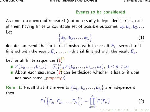
Examples of recurrent events
Ex. 1: Assume a sequence of independent trials with dichotomous(alternative) response, e.g. throws of the coin with P(success) = p.We say that recurrent event ξ appeared in time n if number of successesand failures after n trials are equal.
Ex. 2: Consider particle moving on integer points in the plane. In eachstep particle moves up, down, left or right randomly and independentlyfrom previous steps. Different directions do not have necessarily the sameprobability.We say that recurrent event ξ appeared in time n if we are back instarting point after n steps.
Ex. 3: Consider a particle moving on integer points in the space. In eachstep particle moves up, down, left, right, backwards or forward randomlyand independently from previous steps. Different directions do not havenecessarily the same probability.We say that recurrent event ξ appeared in time n if we are back instarting point after n steps.
J. ANTOCH, KPMS MAI 060 – REMARKS AND EXAMPLES 1. listopadu 2017, 9:16
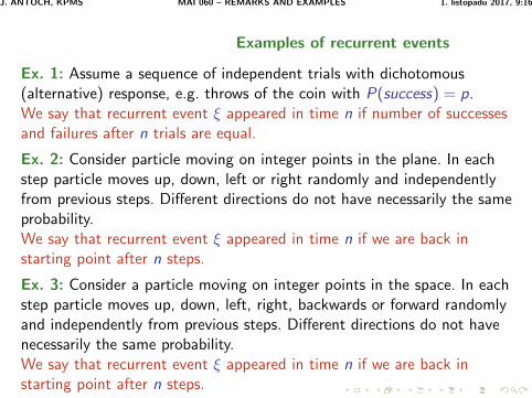
Probabilities un, fn and their interrelation
Def. 3: To each recurrent event ξ there will be assigned two sequencesof numbers
un = P(ξ appeared in the nth trial
)1 ≤ n <∞
fn = P(ξ appeared in the nth trial for the first time
)1 ≤ n <∞
We define formally u0 = 1, f0 = 0 and introduce generating functionsF (x) =
∑∞n=0 fnxn and U(x) =
∑∞n=0 unxn. ♥
Thm. 1: Between probabilities un and fn, respectively betweencorresponding generating functions F (x) and U(x), following relationshold
un = f0un + f1un−1 + . . .+ fnu0 ∀ n ≥ 1
U(x)− 1 = F (x)U(x) − 1 < x < 1
J. ANTOCH, KPMS MAI 060 – REMARKS AND EXAMPLES 1. listopadu 2017, 9:16
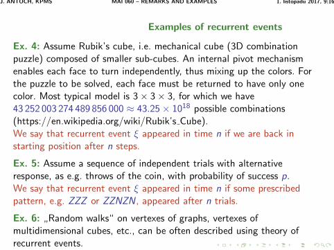
Examples of recurrent events
Ex. 4: Assume Rubik’s cube, i.e. mechanical cube (3D combinationpuzzle) composed of smaller sub-cubes. An internal pivot mechanismenables each face to turn independently, thus mixing up the colors. Forthe puzzle to be solved, each face must be returned to have only onecolor. Most typical model is 3× 3× 3, for which we have43 252 003 274 489 856 000 ≈ 43.25× 10¹⁸ possible combinations(https://en.wikipedia.org/wiki/Rubik’s Cube).We say that recurrent event ξ appeared in time n if we are back instarting position after n steps.
Ex. 5: Assume a sequence of independent trials with alternativeresponse, as e.g. throws of the coin, with probability of success p.We say that recurrent event ξ appeared in time n if some prescribedpattern, e.g. ZZZ or ZZNZN, appeared after n trials.
Ex. 6:”Random walks“ on vertexes of graphs, vertexes of
multidimensional cubes, etc., can be often described using theory ofrecurrent events.
J. ANTOCH, KPMS MAI 060 – REMARKS AND EXAMPLES 1. listopadu 2017, 9:16
Repeated occurrences of recurrent events
Rem. 2:
If f =∑
n fn = 1, then fn corresponds to a random variable T1
describing waiting time for the first occurrence of the event ξ.
If f < 1, then waiting time T1 is so called improper random variable,which with positive probability (= 1− f ) attains improper value ∞,being interpreted as the event that ξ did not came up.
Thm. 2: Denote by f(r)n , 1 ≤ n <∞, probability of the event that ξ
appeared for the r th time in time n, and denote f(r)0 = 0. Then it holds ♥
f(r)n
=
fnr?
Thm. 3: Probability that event ξ will appear in infinitely long sequenceof trials at least r -times is equal to f r , where f =
∑n fn.
J. ANTOCH, KPMS MAI 060 – REMARKS AND EXAMPLES 1. listopadu 2017, 9:16
Repeated occurrences of recurrent events
Rem. 3:
If f =∑
n fn = 1, then fn corresponds to a random variable T1
describing waiting time for the first occurrence of the event ξ.
If f < 1, then waiting time T1 is so called improper random variable,which with positive probability (= 1− f ) attains improper value ∞,being interpreted as the event that ξ did not came up.
Thm. 2: Denote by f(r)n , 1 ≤ n <∞, probability of the event that ξ
appeared for the r th time in time n, and denote f(r)0 = 0. Then it holds ♥
f(r)n
=
fnr?
Thm. 3: Probability that event ξ will appear in infinitely long sequenceof trials at least r -times is equal to f r , where f =
∑n fn.

J. ANTOCH, KPMS MAI 060 – REMARKS AND EXAMPLES 1. listopadu 2017, 9:16
Another way how to introduce recurrent events
Let Ti , 1 ≤ i ≤ r , are independent integer valued rv’s with the samedistribution fn, where Ti is interpreted as the time between (i − 1)-th ai-th occurrence of ξ (so called return time). Then
T (r) = T1 + . . .+ Tr
can be interpreted as waiting time to the r -th occurrence of ξ.
Notion of recurrent event can be introduced in the following way.
Def. 4: First we introduce independent integer valued rv’s T1,T2, . . .with distribution fn and:
statement recurrent event appeared in time n match with thestatement
there exists r such that T1 + T2 + . . .+ Tr = n
statement recurrent event appeared in time n for the r -th timematch with the statement
T1 + T2 + . . .+ Tr = n
J. ANTOCH, KPMS MAI 060 – REMARKS AND EXAMPLES 1. listopadu 2017, 9:16
Classification of recurrent events
Def. 5: An event ξ is called recurrent, if f = 1, respectively transient,if f < 1, where f =
∑n fn.
Thm. 4: Probability, that recurrent event ξ will appear infinitely manytimes in infinitely long series of trials is one for a recurrent event, andzero for a transient event.
Thm. 5: An event ξ is transient if and only if∑∞
n=0 un < +∞. In such acase f = (u − 1)/u, where u =
∑∞n=0 un.
Def. 6: If f = 1, then we denote µ = E T1 =∑∞
n=0 nfn and interpret isas the mean renewal (return) time of ξ.
Def. 7:
An event ξ is called positive recurrent if µ < +∞.An event ξ is called null recurrent if µ = +∞.
Def. 8: An event ξ is called periodical if there exists natural λ > 1 suchthat un = 0 ∀n which are not divisible by λ. Largest λ with this propertyis called a period of ξ.

J. ANTOCH, KPMS MAI 060 – REMARKS AND EXAMPLES 1. listopadu 2017, 9:16
Examples of recurrent events
Ex. 7: Assume a sequence of independent trials with dichotomous(yes/no) response, where P(yes) = p. We say that recurrent event ξappeared in time n if the number of trials which finished yes is equal tothe number of trials that finished no.Show that it is a periodical recurrent event, for which it holds:
if p = 1/2 then ξ is null recurrentif p 6= 1/2 then ξ is transientcalculate probabilities un and fn and their approximationsU(x) =
∑∞n=0
(2nn
)(pqx2
)n= 1√
1−4pqx2
F (x) = 1−√
1− 4pqx2
f2n−1 = 0, f2n = 2n
(2n−2n−1
)pnqn, n = 1, 2, . . .
show that for p = 1/2 it holds un ≈ 1/√πn
simulate couple of random walks of a length at least 105 fordifferent values of p (including p = 1/2)plot corresponding graphs of simulated random walkscompare with Example 1

J. ANTOCH, KPMS MAI 060 – REMARKS AND EXAMPLES 1. listopadu 2017, 9:16
Examples of recurrent events
Ex. 8: Uvazujme castici, ktera se pohybuje po celocıselnych bodechv rovine tak, ze v kazdem kroku se posune o jednotku vlevo, vpravo,nahoru nebo dolu. Vsechny ctyri moznosti jsou stejne pravdepodobnea nezavisle na predchozıch krocıch. Rekneme, ze v case n nastava jev ξ,jestlize jsme se vratili do vychozı pozice. Ukazte, ze se jedna o periodickyrekurentnı jev, ktery je trvaly. Spoctete pravdepodobnosti un a jejichaproximace.
Ex. 9: Uvazujme castici, ktera se pohybuje po celocıselnych bodechv prostoru tak, ze v kazdem kroku se posune o jednotku vlevo, vpravo,nahoru, dolu, dopredu nebo dozadu. Vsechny tyto moznosti jsou stejnepravdepodobne a nezavisle na predchozıch krocıch. Rekneme, ze v case nnastava jev ξ, jestlize jsme se vratili do vychozı pozice. Ukazte, ze sejedna o periodicky rekurentnı jev, ktery je prechodny. Spoctetepravdepodobnosti un a jejich aproximace.
Pomucka. Vzpomente si na multinomicke rozdelenı.
J. ANTOCH, KPMS MAI 060 – REMARKS AND EXAMPLES 1. listopadu 2017, 9:16
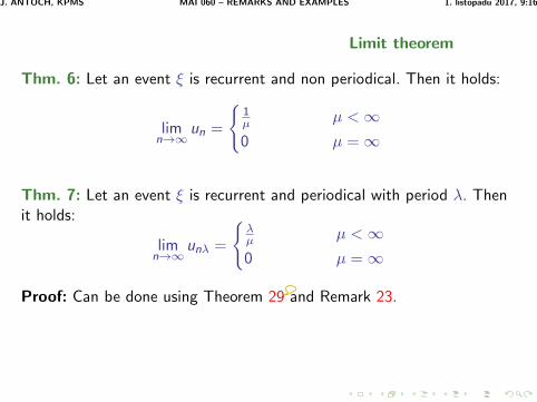
Limit theorem
Thm. 6: Let an event ξ is recurrent and non periodical. Then it holds:
limn→∞
un =
1µ µ <∞0 µ =∞
Thm. 7: Let an event ξ is recurrent and periodical with period λ. Thenit holds:
limn→∞
unλ =
λµ µ <∞0 µ =∞
Proof: Can be done using Theorem 29 and Remark 23.
J. ANTOCH, KPMS MAI 060 – REMARKS AND EXAMPLES 1. listopadu 2017, 9:16
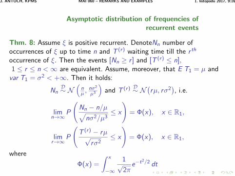
Asymptotic distribution of frequencies ofrecurrent events
Thm. 8: Assume ξ is positive recurrent. DenoteNn number ofoccurrences of ξ up to time n and T (r) waiting time till the r th
occurrence of ξ. Then the events [Nn ≥ r ] and [T (r) ≤ n],1 ≤ r ≤ n <∞ are equivalent. Assume, moreover, that E T1 = µ and
var T1 = σ2 < +∞. Then it holds:
NnD∼ N
(nµ ,
nσ2
µ3
)and T (r) D∼ N
(rµ, rσ2
), i.e.
limn→∞
P
(Nn − n/µ√
nσ2/µ3≤ x
)= Φ(x), x ∈ R1,
limr→∞
P
(T (r) − rµ√
rσ2≤ x
)= Φ(x), x ∈ R1,
where
Φ(x) =
∫ x
−∞
1√2π
e−t2/2 dt
J. ANTOCH, KPMS MAI 060 – REMARKS AND EXAMPLES 1. listopadu 2017, 9:16
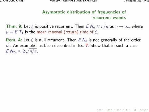
Asymptotic distribution of frequencies ofrecurrent events
Thm. 9: Let ξ is positive recurrent. Then E Nn ≈ n/µ as n→∞, whereµ = E T1 is the mean renewal (return) time of ξ.
Rem. 4: Let ξ is null recurrent. Then E Nn is not generally of the ordern1. An example has been described in Ex. 7. Show that in such a caseE N2n ≈ 2
√n/π.
J. ANTOCH, KPMS MAI 060 – REMARKS AND EXAMPLES 1. listopadu 2017, 9:16
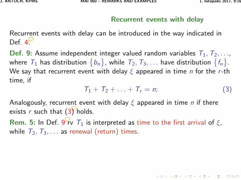
Recurrent events with delay
Recurrent events with delay can be introduced in the way indicated inDef. 4.
Def. 9: Assume independent integer valued random variables T1,T2, . . .,where T1 has distribution
bn
, while T2,T3, . . . have distribution
fn
.We say that recurrent event with delay ξ appeared in time n for the r -thtime, if
T1 + T2 + . . .+ Tr = n; (3)
Analogously, recurrent event with delay ξ appeared in time n if thereexists r such that (3) holds.
Rem. 5: In Def. 9 rv T1 is interpreted as time to the first arrival of ξ,while T2,T3, . . . as renewal (return) times.
J. ANTOCH, KPMS MAI 060 – REMARKS AND EXAMPLES 1. listopadu 2017, 9:16
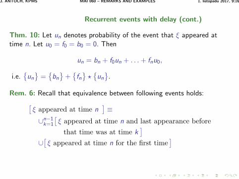
Recurrent events with delay (cont.)
Thm. 10: Let un denotes probability of the event that ξ appeared attime n. Let u0 = f0 = b0 = 0. Then
un = bn + f0un + . . .+ fnu0,
i.e.
un
=
bn
+
fn?
un
.
Rem. 6: Recall that equivalence between following events holds:[ξ appeared at time n
]≡
∪n−1k=1
[ξ appeared at time n and last appearance before
that time was at time k]
∪[ξ appeared at time n for the first time
]
J. ANTOCH, KPMS MAI 060 – REMARKS AND EXAMPLES 1. listopadu 2017, 9:16
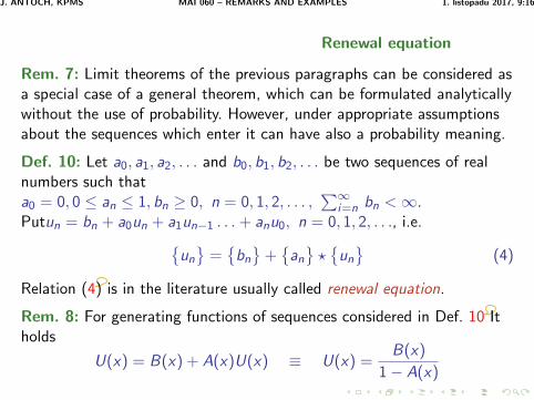
Renewal equation
Rem. 7: Limit theorems of the previous paragraphs can be considered asa special case of a general theorem, which can be formulated analyticallywithout the use of probability. However, under appropriate assumptionsabout the sequences which enter it can have also a probability meaning.
Def. 10: Let a0, a1, a2, . . . and b0, b1, b2, . . . be two sequences of realnumbers such thata0 = 0, 0 ≤ an ≤ 1, bn ≥ 0, n = 0, 1, 2, . . . ,
∑∞i=n bn <∞.
Putun = bn + a0un + a1un−1 . . .+ anu0, n = 0, 1, 2, . . ., i.e.un
=
bn
+
an?
un
(4)
Relation (4) is in the literature usually called renewal equation.
Rem. 8: For generating functions of sequences considered in Def. 10 Itholds
U(x) = B(x) + A(x)U(x) ≡ U(x) =B(x)
1− A(x)
J. ANTOCH, KPMS MAI 060 – REMARKS AND EXAMPLES 1. listopadu 2017, 9:16
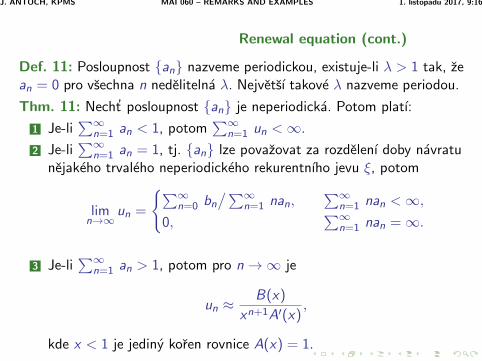
Renewal equation (cont.)
Def. 11: Posloupnost an nazveme periodickou, existuje-li λ > 1 tak, zean = 0 pro vsechna n nedelitelna λ. Nejvetsı takove λ nazveme periodou.
Thm. 11: Necht’ posloupnost an je neperiodicka. Potom platı:
1 Je-li∑∞
n=1 an < 1, potom∑∞
n=1 un <∞.
2 Je-li∑∞
n=1 an = 1, tj. an lze povazovat za rozdelenı doby navratunejakeho trvaleho neperiodickeho rekurentnıho jevu ξ, potom
limn→∞
un =
∑∞n=0 bn
/∑∞n=1 nan,
∑∞n=1 nan <∞,
0,∑∞
n=1 nan =∞.
3 Je-li∑∞
n=1 an > 1, potom pro n→∞ je
un ≈B(x)
xn+1A′(x),
kde x < 1 je jediny koren rovnice A(x) = 1.
J. ANTOCH, KPMS MAI 060 – REMARKS AND EXAMPLES 1. listopadu 2017, 9:16
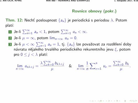
Rovnice obnovy (pokr.)
Thm. 12: Necht’ posloupnost an je periodicka s periodou λ. Potomplatı:
1 Je-li∑∞
n=1 an < 1, potom∑∞
n=1 un <∞.
2 Je-li µ =∞, potom limn→∞ un = 0.
3 Je-li µ <∞∑∞
n=1 an = 1, tj. an lze povazovat za rozdelenı dobynavratu nejakeho trvaleho periodickeho rekurentnıho jevu ξ, potompro 0 ≤ j < λ platı:
limn→∞
unλ+j =λ∑∞
k=0 bkλ+j
µ& lim
n→∞
1
n
∑n
ν=1uν =
∑∞k=0 bk
µ.
J. ANTOCH, KPMS MAI 060 – REMARKS AND EXAMPLES 1. listopadu 2017, 9:16
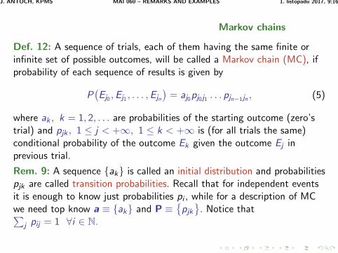
Markov chains
Def. 12: A sequence of trials, each of them having the same finite orinfinite set of possible outcomes, will be called a Markov chain (MC), ifprobability of each sequence of results is given by
P(Ej0 ,Ej1 , . . . ,Ejn
)= aj0pj0j1 . . . pjn−1jn , (5)
where ak , k = 1, 2, . . . are probabilities of the starting outcome (zero’strial) and pjk , 1 ≤ j < +∞, 1 ≤ k < +∞ is (for all trials the same)conditional probability of the outcome Ek given the outcome Ej inprevious trial.
Rem. 9: A sequence ak is called an initial distribution and probabilitiespjk are called transition probabilities. Recall that for independent eventsit is enough to know just probabilities pi , while for a description of MCwe need top know a ≡ ak and P ≡
pjk
. Notice that∑
j pij = 1 ∀i ∈ N.
J. ANTOCH, KPMS MAI 060 – REMARKS AND EXAMPLES 1. listopadu 2017, 9:16
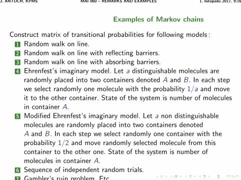
Examples of Markov chains
Construct matrix of transitional probabilities for following models :
1 Random walk on line.2 Random walk on line with reflecting barriers.3 Random walk on line with absorbing barriers.4 Ehrenfest’s imaginary model. Let a distinguishable molecules are
randomly placed into two containers denoted A and B. In each stepwe select randomly one molecule with the probability 1/a and moveit to the other container. State of the system is number of moleculesin container A.
5 Modified Ehrenfest’s imaginary model. Let a non distinguishablemolecules are randomly placed into two containers denotedA and B. In each step we select randomly one container with theprobability 1/2 and move randomly selected molecule from thiscontainer to the other one. State of the system is number ofmolecules in container A.
6 Sequence of independent random trials.7 Gambler’s ruin problem. Etc.
J. ANTOCH, KPMS MAI 060 – REMARKS AND EXAMPLES 1. listopadu 2017, 9:16
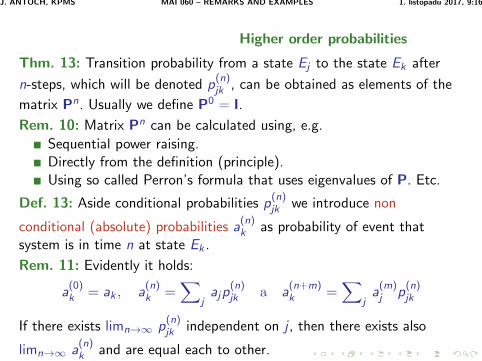
Higher order probabilities
Thm. 13: Transition probability from a state Ej to the state Ek after
n-steps, which will be denoted p(n)jk , can be obtained as elements of the
matrix Pn. Usually we define P0 = I.
Rem. 10: Matrix Pn can be calculated using, e.g.
Sequential power raising.Directly from the definition (principle).Using so called Perron’s formula that uses eigenvalues of P. Etc.
Def. 13: Aside conditional probabilities p(n)jk we introduce non
conditional (absolute) probabilities a(n)k as probability of event that
system is in time n at state Ek .
Rem. 11: Evidently it holds:
a(0)k = ak , a
(n)k =
∑j
ajp(n)jk a a
(n+m)k =
∑j
a(m)j p
(n)jk
If there exists limn→∞ p(n)jk independent on j , then there exists also
limn→∞ a(n)k and are equal each to other.
J. ANTOCH, KPMS MAI 060 – REMARKS AND EXAMPLES 1. listopadu 2017, 9:16
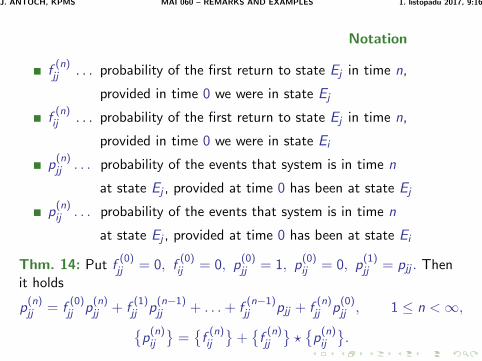
Notation
f(n)jj . . . probability of the first return to state Ej in time n,
provided in time 0 we were in state Ej
f(n)ij . . . probability of the first return to state Ej in time n,
provided in time 0 we were in state Ei
p(n)jj . . . probability of the events that system is in time n
at state Ej , provided at time 0 has been at state Ej
p(n)ij . . . probability of the events that system is in time n
at state Ej , provided at time 0 has been at state Ei
Thm. 14: Put f(0)jj = 0, f
(0)ij = 0, p
(0)jj = 1, p
(0)ij = 0, p
(1)jj = pjj . Then
it holds
p(n)jj = f
(0)jj p
(n)jj + f
(1)jj p
(n−1)jj + . . .+ f
(n−1)jj pjj + f
(n)jj p
(0)jj , 1 ≤ n <∞,
p(n)ij
=
f(n)ij
+
f(n)jj
?
p(n)ij
.

J. ANTOCH, KPMS MAI 060 – REMARKS AND EXAMPLES 1. listopadu 2017, 9:16
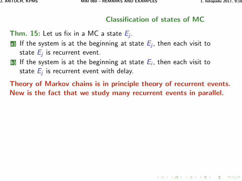
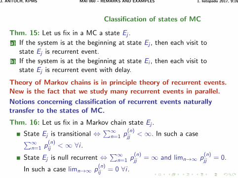
Classification of states of MC
Thm. 15: Let us fix in a MC a state Ej .
a) If the system is at the beginning at state Ej , then each visit tostate Ej is recurrent event.
b) If the system is at the beginning at state Ei , then each visit tostate Ej is recurrent event with delay.
Theory of Markov chains is in principle theory of recurrent events.New is the fact that we study many recurrent events in parallel.
Notions concerning classification of recurrent events naturallytransfer to the states of MC.
Thm. 16: Let us fix in a Markov chain state Ej .
State Ej is transitional ⇔∑∞
n=1 p(n)jj <∞. In such a case∑∞
n=1 p(n)ij <∞ ∀i .
State Ej is null recurrent ⇔∑∞
n=1 p(n)jj =∞ and limn→∞ p
(n)jj = 0.
In such a case limn→∞ p(n)ij = 0 ∀i .
J. ANTOCH, KPMS MAI 060 – REMARKS AND EXAMPLES 1. listopadu 2017, 9:16
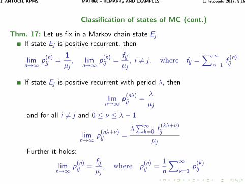
Classification of states of MC (cont.)
Thm. 17: Let us fix in a Markov chain state Ej .
If state Ej is positive recurrent, then
limn→∞
p(n)jj =
1
µj, lim
n→∞p(n)ij =
fijµj, i 6= j , where fij =
∑∞
n=1f(n)ij
If state Ej is positive recurrent with period λ, then
limn→∞
p(nλ)jj =
λ
µj
and for all i 6= j and 0 ≤ ν ≤ λ− 1
limn→∞
p(nλ+ν)ij =
λ∑∞
k=0 f(kλ+ν)ij
µj
Further it holds:
limn→∞
p(n)ij =
fijµj, where p
(n)ij =
1
n
∑∞
k=1p(k)ij
J. ANTOCH, KPMS MAI 060 – REMARKS AND EXAMPLES 1. listopadu 2017, 9:16
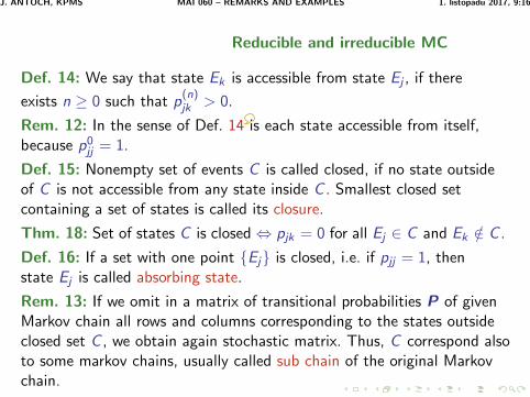
Reducible and irreducible MC
Def. 14: We say that state Ek is accessible from state Ej , if there
exists n ≥ 0 such that p(n)jk > 0.
Rem. 12: In the sense of Def. 14 is each state accessible from itself,because p0
jj = 1.
Def. 15: Nonempty set of events C is called closed, if no state outsideof C is not accessible from any state inside C . Smallest closed setcontaining a set of states is called its closure.
Thm. 18: Set of states C is closed⇔ pjk = 0 for all Ej ∈ C and Ek /∈ C .
Def. 16: If a set with one point Ej is closed, i.e. if pjj = 1, thenstate Ej is called absorbing state.
Rem. 13: If we omit in a matrix of transitional probabilities P of givenMarkov chain all rows and columns corresponding to the states outsideclosed set C , we obtain again stochastic matrix. Thus, C correspond alsoto some markov chains, usually called sub chain of the original Markovchain.

J. ANTOCH, KPMS MAI 060 – REMARKS AND EXAMPLES 1. listopadu 2017, 9:16
Reducible and irreducible MC (cont.)
Def. 17: MC is called irreducible, if is does not contain aside the set ofall states another closed set of states. Otherwise it is called reducible.
Thm. 19: MC is irreducible ⇔ each of its states is accessible from anyother state.
Thm. 20: Markov chain with finitely many states is reducible ⇔corresponding matrix of transitional probabilities P can be, after eventualrenumeration of states, written in the form
P =
(P1 0A B
)where on diagonal we have square matrices.
Rem. 14: We say that states Ej and Ek are of the same type, if both aretransient, or both are null recurrent or positive recurrent, and in parallelare both either periodical or non periodical wit the same period λ.

J. ANTOCH, KPMS MAI 060 – REMARKS AND EXAMPLES 1. listopadu 2017, 9:16
Reducible and irreducible MC (cont.)
Thm. 21: If state Ek is accessible from state Ej and state Ej is accessiblefrom state Ek , then they are of the same type.
Thm. 22: In irreducible MC are all the states of the same type.
Thm. 23: In MC with finitely many states there does not exist nullstates and it is not possible, that all states are transitional ones.
J. ANTOCH, KPMS MAI 060 – REMARKS AND EXAMPLES 1. listopadu 2017, 9:16
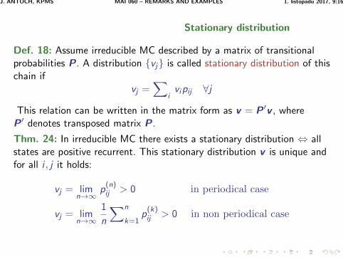
Stationary distribution
Def. 18: Assume irreducible MC described by a matrix of transitionalprobabilities P. A distribution vj is called stationary distribution of thischain if
vj =∑
ivipij ∀j
This relation can be written in the matrix form as v = P ′v , whereP ′ denotes transposed matrix P.
Thm. 24: In irreducible MC there exists a stationary distribution ⇔ allstates are positive recurrent. This stationary distribution v is unique andfor all i , j it holds:
vj = limn→∞
p(n)ij > 0 in periodical case
vj = limn→∞
1
n
∑n
k=1p(k)ij > 0 in non periodical case
J. ANTOCH, KPMS MAI 060 – REMARKS AND EXAMPLES 1. listopadu 2017, 9:16
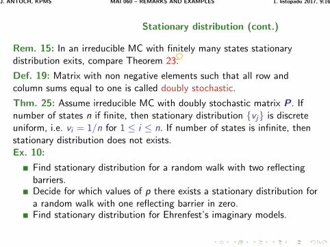
Stationary distribution (cont.)
Rem. 15: In an irreducible MC with finitely many states stationarydistribution exits, compare Theorem 23.
Def. 19: Matrix with non negative elements such that all row andcolumn sums equal to one is called doubly stochastic.
Thm. 25: Assume irreducible MC with doubly stochastic matrix P. Ifnumber of states n if finite, then stationary distribution vj is discreteuniform, i.e. vi = 1/n for 1 ≤ i ≤ n. If number of states is infinite, thenstationary distribution does not exists.Ex. 10:
Find stationary distribution for a random walk with two reflectingbarriers.Decide for which values of p there exists a stationary distribution fora random walk with one reflecting barrier in zero.Find stationary distribution for Ehrenfest’s imaginary models.
J. ANTOCH, KPMS MAI 060 – REMARKS AND EXAMPLES 1. listopadu 2017, 9:16
Basic characterizations of random variables
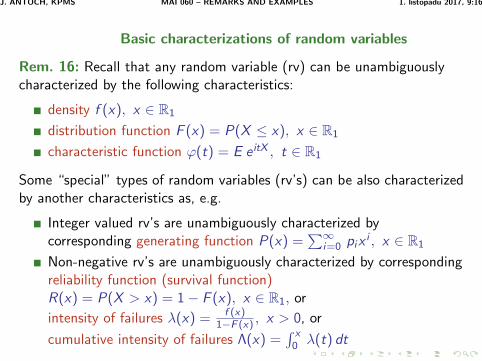
Rem. 16: Recall that any random variable (rv) can be unambiguouslycharacterized by the following characteristics:
density f (x), x ∈ R1
distribution function F (x) = P(X ≤ x), x ∈ R1
characteristic function ϕ(t) = E e itX , t ∈ R1
Some “special” types of random variables (rv’s) can be also characterizedby another characteristics as, e.g.
Integer valued rv’s are unambiguously characterized bycorresponding generating function P(x) =
∑∞i=0 pix
i , x ∈ R1
Non-negative rv’s are unambiguously characterized by correspondingreliability function (survival function)R(x) = P(X > x) = 1− F (x), x ∈ R1, or
intensity of failures λ(x) = f (x)1−F (x) , x > 0, or
cumulative intensity of failures Λ(x) =∫ x0 λ(t) dt
J. ANTOCH, KPMS MAI 060 – REMARKS AND EXAMPLES 1. listopadu 2017, 9:16
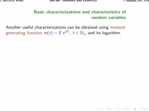
Basic characterizations and characteristics ofrandom variables
Another useful characterizations can be obtained using momentgenerating function m(t) = E etX , t ∈ R1, and its logarithm.
J. ANTOCH, KPMS MAI 060 – REMARKS AND EXAMPLES 1. listopadu 2017, 9:16
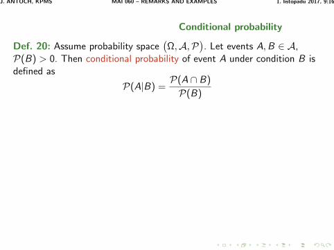
Conditional probability
Def. 20: Assume probability space(Ω,A,P
). Let events A,B ∈ A,
P(B) > 0. Then conditional probability of event A under condition B isdefined as
P(A|B) =P(A ∩ B)
P(B)

J. ANTOCH, KPMS MAI 060 – REMARKS AND EXAMPLES 1. listopadu 2017, 9:16
Conditional characteristics for discrete rv’s
Def. 21: Let X and Y are two discrete rv’s. Then:
conditional density of X given that Y = y is defined by
pX |Y (x |y) = P(X = x |Y = y
)=P(X = x ,Y = y
)P(Y = y
) =pX ,Y (x , y)
pY (y)
conditional distribution function of X given that Y = y is defined by
FX |Y (x |y) = P(X ≤ x |Y = y
)=∑z≤x
pX |Y (z |y)
conditional expectation of X given that Y = y is defined by
E[
X |Y = y]
=∑x
x · P(X = x |Y = y
)=∑x
x · pX |Y (x |y)
conditional variance of X given that Y = y is defined by
var[
X |Y = y]
= E[(
X − E[
X |Y = y])2|Y = y
]
J. ANTOCH, KPMS MAI 060 – REMARKS AND EXAMPLES 1. listopadu 2017, 9:16
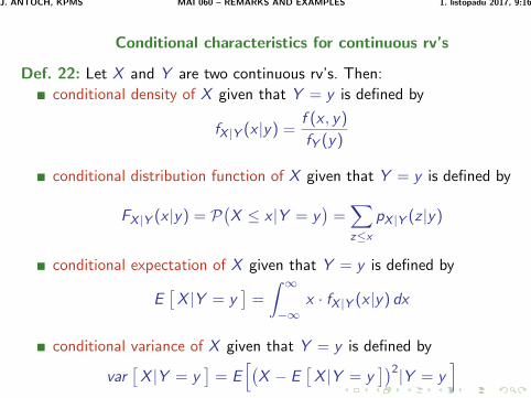
Conditional characteristics for continuous rv’s
Def. 22: Let X and Y are two continuous rv’s. Then:
conditional density of X given that Y = y is defined by
fX |Y (x |y) =f (x , y)
fY (y)
conditional distribution function of X given that Y = y is defined by
FX |Y (x |y) = P(X ≤ x |Y = y
)=∑z≤x
pX |Y (z |y)
conditional expectation of X given that Y = y is defined by
E[
X |Y = y]
=
∫ ∞−∞
x · fX |Y (x |y) dx
conditional variance of X given that Y = y is defined by
var[
X |Y = y]
= E[(
X − E[
X |Y = y])2|Y = y
]
J. ANTOCH, KPMS MAI 060 – REMARKS AND EXAMPLES 1. listopadu 2017, 9:16
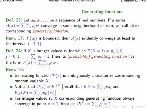
Generating functions
Def. 23: Let a0, a1, . . . be a sequence of real numbers. If a seriesA(x) =
∑∞j=0 ajx
j converge in some neighborhood of zero, we call A(x)corresponding generating function.
Rem. 17: If aj is bounded, then A(x) evidently converge at least inthe interval (−1, 1).
Def. 24: If X is integer valued rv for which P(X = j) = pj ≥ 0,j = 0, 1, . . . ,
∑j pj = 1, then its (probability) generating function has
the form P(x) =∑∞
j=0 pjxj .
Rem. 18:
Generating function P(x) unambiguously characterize correspondingrandom variable X .
Notice that P(t) = E tX[recall that E X =
∑j pjxj and
E g(X ) =∑
j pjg(xj)].
For integer valued rv X corresponding generating function alwaysconverge in point x = 1, because P(1) =
∑j pj = 1.

J. ANTOCH, KPMS MAI 060 – REMARKS AND EXAMPLES 1. listopadu 2017, 9:16
Generating functions – examples
Ex. 11: Check the form of generating functions for following mostimportant discrete distributions:
Alternative . . . P(x) = q + px
Binomial . . . P(x) = (q + px)n
Poisson . . . P(x) = exp−λ+ λxGeometrical . . . P(x) = p/(1− qx)
resp. = px/(1− qx)
Negative binomial . . . P(x) =(p/(1− qx)
)rresp. =
(px/(1− qx)
)rDiscrete uniform . . . P(x) = (1− xn+1)/
((n + 1)(1− x)
)resp. =
(x(1− xn)
)/(n(1− x)
)Using these generating functions calculate corresponding expectationsand variances.
Rem. 19: Recall that geometric and negative binomial distributions arethe simplest models describing waiting times.
J. ANTOCH, KPMS MAI 060 – REMARKS AND EXAMPLES 1. listopadu 2017, 9:16
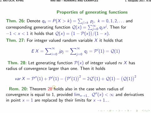
Properties of generating functions
Thm. 26: Denote qk = P(X > k) =∑
j>k pj , k = 0, 1, 2, . . . and
corresponding generating function Q(x) =∑∞
j=0 qjxj . Then for
−1 < x < 1 it holds that Q(x) =(1− P(x)
)/(1− x).
Thm. 27: For integer valued random variable X it holds that
E X =∑∞
i=0jpj =
∑∞
j=0qj = P ′(1) = Q(1)
Thm. 28: Let generating function P(x) of integer valued rv X hasradius of convergence larger than one. Then it holds
var X = P ′′(1) + P ′(1)−(P ′(1)
)2= 2Q′(1) +Q(1)−
(Q(1)
)2Rem. 20: Theorem 28 holds also in the case when radius of
convergence is equal to 1, provided limx→1− Q′′(x) <∞ and derivativesin point x = 1 are replaced by their limits for x → 1−.
J. ANTOCH, KPMS MAI 060 – REMARKS AND EXAMPLES 1. listopadu 2017, 9:16
Partial fraction decomposition
Rem. 21: Knowledge of P(x) is theoretically equivalent to knowledge ofpj, and vice versa. However, the use of the fact that pj = P(j)(0)/j!can be quite complicated in practice. In such a case followingapproximation can be useful.
Thm. 29: Let generating function P(x) of the sequence pn can bewritten in the form P(x) = U(x)/V (x), where U(x) and V (x) arepolynomials without common roots, order of U(x) is smaller than orderof V (x), and the roots of polynomial V (x) are simple. Then
pn =ρ1
xn+11
+ · · ·+ ρm
xn+1m
, 0 ≤ n <∞,
where m is order of polynomial V (x), x1, . . . , xm are its roots andρk = −U(xk)/V ′(xk), 1 ≤ k ≤ m.
Rem. 22: For calculation of ρk is usually used decomposition into partialfractions, embedded in programs Maple or Mathematica, e.g.
J. ANTOCH, KPMS MAI 060 – REMARKS AND EXAMPLES 1. listopadu 2017, 9:16
Partial fraction decomposition
Rem. 23: Assume that x1 is that root of V (x) for which|x1| < xk , 2 ≤ k ≤ m. Then
pn =ρ1
xn+11
(1 +
ρ2ρ1
(x1x2
)n+1+ . . .+
ρmρ1
( x1xm
)n+1), (6)
so that for n→∞ it holds that pn ≈ ρ1/xn+11 , where
ρ1 = −U(x1)/V ′(x1).
Rem. 24: For validity of the assertion pn ≈ ρ1/xn+11 it is possible to
omit assumption that degree of U(x) is smaller than degree of V (x).Instead it is sufficient to assume only that the root x1 is unique.Moreover, recall that practical experience shows that theapproximation (6) is satisfactory even for small values of n.
Ex. 12: Let qn be probability that in the sequence of n trials withdichotomous response (T,F ) a subsequence FFF will not appear. Findcorresponding generating function and calculate correspondingprobabilities qn both precisely and using the above approximations.Solution: Q(x) =
(8 + 4x + 2x2
)/(8− 4x − 2x2 − x3
).

J. ANTOCH, KPMS MAI 060 – REMARKS AND EXAMPLES 1. listopadu 2017, 9:16
Convolution
Def. 25: Let a0, a1, . . . a b0, b1, . . . are two sequences of real numbers.Then a sequence c0, c1, . . . defined by relation
cn = a0bn + a1bn−1 + . . .+ anb0, n = 0, 1, . . .is called convolution of sequences aj and bj. We will writecj = aj ? bj.
Thm. 30: Let aj and bj are two sequences with generating functionsA(x) and B(x). Then for the generating function corresponding to theirconvolution cj it holds
C(x) = A(x)B(x).Rem. 25: Convolution of a sequence aj with itself is called convolutionpower and is denoted aj2?. Analogously, n-th convolution poweraj ? . . . ? ajwill be denoted ajn?.
J. ANTOCH, KPMS MAI 060 – REMARKS AND EXAMPLES 1. listopadu 2017, 9:16
Convolution
Thm. 31: Let X1,X2, . . . ,Xn are independent identically distributed (iid)rv’s with integer valued distribution described by probabilities pj.Denote corresponding generating function by P(x). Then distribution oftheir sum, i.e. distribution of X1 + X2 + . . .+ Xn is described by the n-thconvolution power pjn?, and corresponding generating function has theform
P(x) . . .P(x) = Pn(x)
J. ANTOCH, KPMS MAI 060 – REMARKS AND EXAMPLES 1. listopadu 2017, 9:16
Compound distributions
Thm. 32: Let X1,X2, . . . and N are independent integer valued rv’s,Xi ’s have the same distribution fj and N has distribution gj.Then SN = X1 + . . .+ XN is also integer valued random variable with thedistribution hj, where
hj = P(SN = j) =∑∞
n=0gn · fjn?.
If A(x),B(x) and C(x) are generating functions corresponding to thesequences fj, gj and hj, then C(x) = B
(A(x)
)and
E SN = E X1 · E N. Corresponding variance o can be calculated usingTheorem 28.
Rem. 26: Notice that random variable SN = X1 + . . .+ XN is nothingelse than random sum of random variables.
Ex. 13: Let number N of laid eggs follow Poisson distribution Po(λ) andprobability of arrival of individual from an egg is p, i.e. Xi followalternative distribution. Show that in such a case SN follows Poissondistribution Po(λ · p).