Magnetosphereionosphere energy interchange in … energy interchange in the electron diffuse ... energy interchange in the electron diffuse aurora, J ... spirals, are pitch angle

JOURNAL OF GEOPHYSICAL RESEARCH: SPACE PHYSICS, VOL. 119, 1–14, doi:10.1002/2013JA019325, 2014

Magnetosphere-ionosphere energy interchange in the electron

diffuse aurora

G. V. Khazanov,1 A. Glocer,1 and E. W. Himwich2,1

Received 15 August 2013; revised 2 December 2013; accepted 4 December 2013.

[1] The diffuse aurora has recently been shown to be a major contributor of energy fluxinto the Earth’s ionosphere. Therefore, a comprehensive theoretical analysis is required tounderstand its role in energy redistribution in the coupled ionosphere-magnetospheresystem. In previous theoretical descriptions of precipitated magnetospheric electrons(E � 1 keV), the major focus has been the ionization and excitation rates of the neutralatmosphere and the energy deposition rate to thermal ionospheric electrons. However,these precipitating electrons will also produce secondary electrons via impact ionizationof the neutral atmosphere. This paper presents the solution of the Boltzman-Landaukinetic equation that uniformly describes the entire electron distribution function in thediffuse aurora, including the affiliated production of secondary electrons (E < 600 eV) andtheir ionosphere-magnetosphere coupling processes. In this article, we discuss for the firsttime how diffuse electron precipitation into the atmosphere and the associated secondaryelectron production participate in ionosphere-magnetosphere energy redistribution.Citation: Khazanov, G. V., A. Glocer, and E. W. Himwich (2014), Magnetosphere-ionosphere energy interchange in the electrondiffuse aurora, J. Geophys. Res. Space Physics, 119, doi:10.1002/2013JA019325.

1. Introduction

[2] In the theoretical description of precipitated magne-tospheric electrons in regions of diffuse aurora, the majorfocus was always on the ionization and excitation rates ofthe neutral atmosphere, and/or heating of the thermal plasma[Rees, 1989]. A number of different approaches to the solu-tion of the transport equation in the auroral ionosphere arepresented in literature. Electron transport models for Earth’saurora have been developed by using a two-stream approach[Banks et al., 1974], using a multistream approach thatgives the details of pitch angle resolution [Strickland et al.,1976] , using numerical implementation of the Boltzman-Landau kinetic equation [Khazanov, 1979], using a two-stream discrete ordinate method [Stamnes, 1981], applyinga Feautrier solution [Link, 1992], using a discrete ordi-nate technique [Lummerzheim and Lilensten, 1994], andusing a Monte Carlo technique [Solomon, 1993]. Min et al.[1993] took the discrete ordinate method of Lummerzheimand Lilensten [1994] to include small field-aligned iono-spheric electric fields in order to study the influence of theambipolar diffusion field on electron precipitation. Peticolasand Lummerzheim [2000] have developed a time-dependentelectron transport model, which can simulate flickeringaurora or fast moving auroral filaments.

1NASA GSFC, Greenbelt, Maryland, USA.2Yale University, New Haven, Connecticut, USA.

Corresponding author: G. V. Khazanov, NASA/GSFC, Code 673,Greenbelt, MD 20771, USA. ([email protected])

©2013. American Geophysical Union. All Rights Reserved.2169-9380/14/10.1002/2013JA019325

[3] The global energy input into the atmosphere in thediffuse zone of the polar lights is substantially larger thanthe energy input associated with localized discrete auroralarcs. It turns out that the diffuse aurora, which is alwayspresent and widely distributed in rings around Earth’s mag-netic poles, collectively accounts for about three-quarters ofthe auroral energy precipitating into the ionosphere [e.g.,Newell et al., 2009]. The global pattern of electron pre-cipitation can dramatically change the conductivity of theionosphere, which can in turn influence the global patternof magnetospheric convection, which are all affiliated withionosphere-magnetosphere coupling processes [Khazanovet al., 2003]. For this reason, diffuse auroral precipitationneeds to be included in the development of global modelsfor the Earth’s magnetosphere.

[4] The diffuse aurora is characterized by a broad andfairly stable emission [Lui and Anger, 1973] and is thoughtto result from the precipitation of electrons that are notaccelerated in the direction parallel to a magnetic field [e.g.,Winningham et al., 1975; Lui et al., 1977; Meng et al.,1979; Fontaine and Blanc, 1983; Schumaker et al., 1989;Johnstone et al., 1993].

[5] Diffuse precipitation of energetic electrons from themagnetosphere is a consequence of pitch angle scatteringby plasma waves. In particular, it is expected that the dif-fuse aurora is caused by hot plasma sheet electrons that arepitch angle scattered into the loss cone by whistler modewaves near the equatorial plane [e.g., Kennel and Petschek,1966; Lyons, 1974; Johnstone et al., 1993]. These electronsare assumed to then precipitate into the atmosphere with-out further acceleration at high latitudes [e.g., Winninghamet al., 1975; Lui et al., 1977; Meng et al., 1979; Fontaineand Blanc, 1983; Schumaker et al., 1989; Johnstone et al.,

1

https://ntrs.nasa.gov/search.jsp?R=20140017833 2018-07-17T09:13:20+00:00Z

KHAZANOV ET AL.: I-M ENERGY INTERCHANGE

1993] and result a broad and fairly stable emission [Lui andAnger, 1973]. Diffuse auroral precipitation occurs over abroad range of geomagnetic latitudes that map along fieldlines from the inner magnetosphere and the plasma sheet,which is basically the region of closed magnetic field lines.Depending on the intensity of the geomagnetic storms, themagnetospheric electron precipitation can even reach mag-netic latitudes � 50ı–55ı. The precipitation of energeticelectrons in the diffuse auroral region is an important sourceof ionizing energy input to the middle atmosphere and heat-ing of the thermal plasma. The strongest diffuse auroras arefound on the postmidnight sector, while proton precipitationis important especially in the premidnight sector [Nishimuraet al., 2013]. The detailed morphology of the phenomena ofprecipitated magnetospheric electrons, as well as a compre-hensive list of related studies, were presented by Hardy et al.[1987], and more recently by Newell et al. [2009, 2010].

[6] Secondary electrons (with energies below 500–600 eV)are produced by collisions of primary electrons of thediffuse aurora with the neutral atmosphere. The observa-tional evidence for secondary electrons in the past has beendiscussed by Frank and Ackerson [1971], Arnoldy et al.[1974], and Evans [1974]; more recently, numerous DefenseMeteorological Satellite Program (DMSP) observationsrelated to various types of auroral events have been sum-marized by Newell et al. [2009, 2010]. These secondariescan escape back to the magnetosphere, can be trapped onclosed magnetic field lines, and can deposit their energyback to the inner magnetosphere. As far as we know, therehas been no prior study focusing on the aspect of diffuseauroral magnetosphere-ionosphere energy interchange thatis affiliated with secondary electron production in this regionand the escape of these secondary electrons back to themagnetosphere and conjugate ionosphere.

[7] Our study focuses on the magnetosphere-ionosphereenergy interchange in the diffuse auroral region and isdesigned to answer the following question: How do dif-fuse auroral electron precipitation, with initial energies E >600 eV, and the affiliated secondary electron population thatit produces participate in ionosphere-magnetosphere energyand particle redistributions via different kinds of collisionalprocesses with neutral and charged particles?

[8] This paper is organized as follows: The physical sce-nario of our simulations are discussed in section 2; themathematical formalism and the numerical implementationof our superthermal electron model are briefly outlined insection 3; all results are presented in section 4; and finally,section 5 provides the summary and conclusions.

2. Physical Scenario

[9] The diffuse aurora occurs over a broad latitude rangeof � = 55ı–70ı and is primarily caused by the precip-itation of low-energy (0.5–30 keV) electrons originatingin the central plasma sheet. A more precise and definitiverelation between diffuse auroras and their particle sourceregion was determined by simultaneous examination of theparticle observations at geosynchronous orbit, the auroraldisplay, and the auroral electron precipitation near its con-jugate field line observed by the polar-orbiting DMSP 32satellite and presented by Meng et al. [1979]. It was foundthat the spectral shape and differential fluxes of electrons

precipitated in diffuse auroras were very similar, and some-times almost identical, to those of the trapped plasma sheetelectrons located simultaneously in the conjugate magneto-spheric equator. The characteristics of auroral electron pre-cipitation are therefore determined by the particle features inthe conjugate magnetospheric equator and the diffuse aurorais produced by the direct dumping of plasma sheet electrons.This similarity of characteristics shows indirect evidence forthe absence of parallel electric fields in the region of electrondiffuse aurora and it is expected that diffuse electron precipi-tation occurs simultaneously in both magnetically conjugateionospheres.

[10] In terms of visual auroral morphology, the aboveidentification implies that discrete auroras are produced byelectrons from boundaries of the plasma sheet and diffuseauroras by electrons from the central plasma sheet, theearthward edge of the plasma sheet, and/or the outer radia-tion zone [Ebihara et al., 2010]. The close relation betweenthe diffuse aurora and plasma sheet electrons has been dis-cussed [Eather and Mende, 1971; Hoffman and Burch, 1973;Lui et al., 1977].

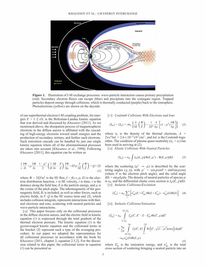
[11] Based on the discussion above, Figure 1 presents thephysical scenario of our simulation of the energy exchangedbetween the magnetosphere and ionosphere during magne-tospheric electron precipitation events into the two magnet-ically conjugate ionospheric regions including the affiliatedproduction of secondary electrons (E < 600 eV), their escapeback to the magnetosphere, their trapping on closed mag-netic field lines, and their deposition of energy to thermalmagnetospheric electrons.

[12] In Figure 1, we show this energy interchange on boththe dayside and nightside of the space plasma. First, weillustrate the production of precipitating fluxes in the plasmasheet, shown as an orange cloud, where hot electrons, shownas tight orange spirals, are pitch angle scattered by whistlermode waves, shown in gray. The symmetrically precipitat-ing primary electrons, entering into the conjugate northernand southern ionospheres, are shown by red arrows labeledPrecipitating Primary Flux.

[13] The secondary electron flux (E < 600 eV) caused bythis primary precipitation is shown by blue arrows labeledEscaping Secondary Flux. Blue spirals show the escapingparticles that move along the magnetic field, some por-tion of which become trapped, illustrated by a blue cloud,and deposit energy to thermal electrons via Coulomb col-lisional processes. The conduction of this energy back tothe ionosphere is shown by purple arrows labeled ReturnedThermal Flux.

[14] The dayside of Figure 1 also shows, in yellow, theproduction of photoelectrons. These photoelectrons are pro-duced in the same energy range as secondary electrons andare generated as a result of the interaction of Solar UV andX-ray radiation with the neutral atmosphere. In this paper,both secondary electrons and photoelectrons will be referredto as superthermal electrons (SE) and will be only distin-guished below when we discuss the relative role of thesepopulations in SE production on the dayside.

3. Theoretical Formalism

[15] Now, we consider the theoretical formalism of thephysical scenario that we described above. The starting point

2


Figure 1. Illustration of I-M exchange processes: wave-particle interaction causes primary precipitation(red). Secondary electron fluxes can escape (blue) and precipitate into the conjugate region. Trappedparticles deposit energy through collisions, which is thermally conducted (purple) back to the ionosphere.Photoelectrons (yellow) are shown on the dayside.

of our superthermal electron I-M coupling problem, for ener-gies E > 1–2 eV, is the Boltzman-Landau kinetic equationthat was derived and discussed by Khazanov [2011]. As wementioned above, the dissipation process of magnetosphericelectrons in the diffuse aurora is affiliated with the cascad-ing of high-energy electrons toward small energies and theproduction of secondary, tertiary, and further such electrons.Such ionization cascade can be handled by just one singlekinetic equation where all of the aforementioned processesare taken into account [Khazanov et al., 1994]. FollowingKhazanov [2011], this equation can be written as

1v

@ˆ

@t+�

@ˆ

@s–

1 – �2

2

�1B

@B@s

–FE

�@ˆ

@�+EF�

@

@E

�ˆ

E

�= Q+ hSi

(1)

where ˆ = 2Ef/m2 is the SE flux, f = f(t, s, �, E) is the elec-tron distribution function, v is SE velocity, t is time, s is thedistance along the field line, E is the particle energy, and � isthe cosine of the pitch angle. The inhomogeneity of the geo-magnetic field, B, is included, as well as other forces, such aselectric fields, in F. Q is the SE source term and hSi, whichincludes collision integrals, represents interactions with ther-mal electrons and ions, scattering with neutral particles andwave-particle interactions.

[16] This paper focuses only on the collisional processesin the diffuse electron aurora, and the electric field in kineticequation (1) is expressed through the total gradient of thethermal electron pressure. The kinetic equation (1) is thegyroaveraged kinetic equation and the collisional terms inthe bracket hSi represent such a type of the averaging pro-cedure. In our paper we adopted the representation forall collisional processes in accordance with the book byKhazanov [2011, chapter 2, equation 2.5.2]. For the discus-sion related to this paper, the collisional terms in equation(1) can be presented as

[17] Coulomb Collisions With Electrons and Ions

hSeei + hSeii = Ane

�@

@E

�ˆ

E

�+

12E2

@

@�

�(1 – �2)

@ˆ

@�

��(2)

where ne is the density of the thermal electrons, A =2�e4lnL = 2.6�10–12eV2cm2 , and lnL is the Coulomb loga-rithm. The condition of plasma quasi-neutrality (ne = ni) hasbeen used in arriving at (2).

[18] Elastic Collisions With Neutral Particles

hSeai = n˛

ZI˛(E, �)[ˆ(E, �0) – ˆ(E, �)]d� (3)

where the scattering (�0 ! �) is described by the scat-tering angles (�, �), with �0 = cos�cos� + sin�sin�cos�(where � is the electron pitch angle), and the solid angled� = sin�d�d�. The density of neutral particles of species ˛is n˛ and the differential elastic cross section is I˛(E, �)d�.

[19] Inelastic Collisions/Excitation

hS*eai = n˛

Xj

h*

˛j(E + E*˛j)ˆ(E + E*

˛j) – *˛j(E)ˆ(E)

i(4)

[20] Inelastic Collisions/Ionization

hS+eai = n˛

2E+E+˛Z

E+E+˛

I+˛(E0, E0 – E – E+

˛)ˆ(E0, �)dE0

+n˛

2�

1Z2E+E+

˛

I+2(E0, E)

2�Z0

ˆ�

E0,p

(1 – �2)cos�

d�dE0

– n˛+˛(E)ˆ(E, �)

(5)where E+

˛ is the ionization energy, and *˛j is the total

cross section of scattering bringing a neutral particle into an

3


excited state characterized by a threshold energy E*˛j. We

also have

h+e˛i =

(E–E+˛ )/2Z

0

I+˛(E, E2)dE2

which is the total cross section of ionization by an electronwith energy E. I+

˛(E, E2) is the appropriate differential crosssection and E2 is the energy of a secondary electron.

[21] In order to solve the kinetic equation (1) with col-lision terms presented by equations (2)–(5), we used anumerical method that has been discussed in detail in thebook by Khazanov [2011, in Chapter 7]. This method isbased on a solution to the kinetic equation along the entirelength of a closed magnetic field line that is simultaneousfor the two conjugate ionospheres and the magnetosphere.It allows the determination of the distribution in energy andpitch angle of superthermal electrons along the completelength of the field line, thereby avoiding the introductionof artificial boundaries between the ionosphere and mag-netosphere and consequently avoiding problems introducedby the uncertainty of these boundary conditions. In addi-tion, it automatically accounts for backscattered electrons inthe atmosphere and plasmasphere, and avoids splitting SEinto a loss cone and a trapped population. The method isnot limited to specific situations, such as conjugated sunriseor symmetrical illumination of hemispheres, but is equallyapplicable to arbitrary illumination conditions, including theprecipitation of electrons with magnetospheric origin, aspresented in the scenario shown in Figure 1.

[22] Along a closed magnetic field line in the plasmas-phere, the magnetic field is strongly inhomogeneous, whilecollisional diffusion terms are small due to the long meanfree path. In order to decrease undesirable computationaleffects associated with approximation errors of the deriva-tives @/@s and @/@�, it is convenient to change variables from(�, s) to (�0, s), where

�0 =�

|�|

s1 –

B0

B(s)(1 – �2) (6)

with B0 and �0 denoting the magnetic field and the cosineof the pitch angle at the magnetic equator of the fluxtube. This change of variables is desirable because ˆ(�0, s)now becomes a slowly varying function with s (withoutany external forces, �0 is simply the adiabatic invariant)that greatly reduces computational effects associated withapproximation errors of the derivatives.

[23] The new variable �0 takes on values in the range|�0B| < |�0| < 1, where the lower boundary �0B =p

1 – B0/B(s) is a function of s. A specific feature of the algo-rithm used to solve the kinetic equation (1) in new variables(�0, s) is that the number of grid points in �0 varies withs because the definition interval varies with s. In the mag-netosphere, where the inhomogeneity of the magnetic fieldcauses �0B to vary significantly, the number of steps in �0 isincreased by 2 for each step in s toward the magnetic equator.This scheme is illustrated in the book by Khazanov [2011,Figure 7.1] which shows the adopted grid as a function ofs and �0 = cos–1�0. Since the magnetic field changes littlein the ionosphere, while at the same time the step size in sis smaller in this region, the values �0B of adjacent altitudegrid points would be undesirably close if this scheme was

extended all the way to the base of the ionosphere. Instead,we assume that the magnetic field is homogeneous belowsome altitude s1 (typically 800 km) so that �0B is constant inthe ionosphere.

[24] The number of grid points in the loss cone, �0 =˙p

1 – B0/B(s1), is constant for the complete field line.The trapping region is defined by

p1 – B0/B(s) � |�0| �p

1 – B0/B(s1) and the loss-cone region byp

1 – B0/B(s1) ��0 � 1. The boundary conditions in s are imposed at conju-gate points of the ionosphere, –s2 and +s2 at the altitude of90 km or below (depending on the energy of the precipitatedmagnetospheric electrons) using the local approximation(@/@s = 0).

[25] Using the numerical technique developed byKhazanov et al. [1993, 1994] the kinetic equation has beensolved for these new variables (t, E, �0(�, s), s) under thefollowing initial and boundary conditions:

ˆ(t = 0, s, �0, E) = ‰0(s, �0, E)

(7)

ˆ(t, s = –s1, �0, E) = ‰–(t, �0, E); –1 � �0 � –p

1 – B0/B(–s1)

ˆ(t, s = s1, �0, E) = ‰+(t, �0, E);p

1 – B0/B(s1) � �0 � 1(8)

@ˆ(�0 = 0, �)@�0

= 0; �0 = cos–1�0

(9)ˆ+(t, s, �0 = �0b , E) = ˆ–(t, s, �0 = –�0b , E)

(10)@ˆ+

@�0(t, s, �0 = �0b , E) = –

@ˆ–

@�0(t, s, �0 = –�0b , E)

(11)ˆ(t, s, �0, E = 0; E = Emax) = 0

(12)

where ‰0 is the initial distribution in the flux tube; ‰˙ arethe low altitude (in our case, 90 km) boundary fluxes whichwere calculated from equation (1) for the condition of localequilibrium; and �0 is the equatorial pitch angle. We haveintroduced the boundary conditions at intermediate altitude,800 km, for the precipitated magnetospheric electron fluxeswith the energies E > 600 eV with different initial energyspectra. For the purposes of this paper, we assume that theprecipitated magnetospheric electrons are isotropic in pitchangle over the earthward direction and located at an initialheight of 800 km. The energy distribution of these electronsis Gaussian [Banks et al., 1974]

ˆ(E) = Ce–(E–E0)2/2�2(13)

or Maxwellian [Rees, 1989]

ˆ(E) = CEe–E/E0 (14)

where C is the normalization factor, E0 is the character-istic energy of precipitated magnetospheric electrons, and = 0.1E0 [Banks et al., 1974]. The normalization factorC for equations (13) and (14) has been chosen to representthe energy flux of the precipitated magnetospheric elec-trons to the ionospheric region. Table 1 presents C valuesfor Gaussian (equation (13)) and Maxwellian (equation(14))spectra at the boundary of 800 km that are calculated for the

4


Table 1. Normalization Constant C for Different Spectra, Total Energy Flux 1 erg cm–2 s–1

Mean Energy (keV) 0.4 0.8 1.0 2.0 3.0 5.0

Gaussian spectrum 1.14 � 1013 1.25 � 106 7.94 � 105 1.98 � 105 8.82 � 104 3.17 � 104

Maxwellian spectrum 1.92 � 103 2.02 � 102 1.02 � 102 1.25 � 101 3.95 � 100 7.96 � 10:1

total energy flux of 1 erg cm–2 s–1 for different mean ener-gies, with an assumption that their pitch angle distributionis isotropic in the earthward direction. The Gaussian shapeof the spectra is not very relevant to the precipitated elec-tron flux in the diffuse aurora [Mishin et al., 1990]. We onlyuse such a form in one of the plots below for benchmarkingpurposes in order to emphasize the point of the paper.

[26] To perform the calculations, we used the follow-ing input for our SE model. For the purposes of this study,the Earth’s magnetic field is assumed to be a dipole; how-ever, the numerical algorithm that we developed could beused for any arbitrary magnetic field configuration, whichwill be demonstrated in follow up papers that will compareour model to particle observation results. Solar EUV andX-ray radiation spectra were obtained using the Hintereggeret al. [1981] model, while neutral thermospheric densitiesand temperatures were given by MSIS-90 [Hedin, 1991].The electron profile in the ionosphere was calculated basedon the IRI model [Bilitza, 1990] and extended in the plasma-sphere region using the assumption that the electron thermaldensity distribution in the plasmasphere is proportional tothe geomagnetic field as ne � B2. This case indicates someintermediate step occurring during plasmaspheric refilling[Khazanov et al., 1984] and corresponds to the large L shellswhere electron diffuse aurora is taking place.

[27] Photoabsorption and photoionization cross sectionsfor O, O2, and N2 were taken from Fennelly and Torr [1992].Partial photoionization cross sections for O2 and N2 wereobtained from Conway [1988], while partial photoionizationcross sections of Bell and Stafford [1992] were adopted foratomic oxygen. Cross sections for elastic collisions, state-specific excitation, and ionization were taken from Solomonet al. [1988]. All of the calculations testing the effects ofphotoelectrons were performed for a local time of noon atequinox (midnight when not testing the effect of photoelec-trons), with F10.7 and hF10.7i values of 150, chosen so theatmospheric conditions are symmetric and the solar radiationis at an average intensity level.

4. Results and Discussion

[28] We demonstrate our SE flux calculation in the elec-tron diffuse auroral region for the conditions describedabove with an emphasis on the ionosphere-magnetospherecoupling processes. Specifically, we focus on the energy andparticle flux redistribution between the magnetosphere andthe two magnetically conjugate ionospheres. Our choice of athermal density distribution in the plasmasphere ne � B2 atlarge L shells, L � 5, which is typical for the electron diffuseaurora, caused our flux calculations to be independent of Lshell for L � 5, and all of our results are only presented forL = 6. The thermal density distribution choice of ne � B2 isvery conservative and any effects shown by our calculationwill be amplified for higher thermal densities.

[29] We first present our modeled SE omnidirectionalfluxes at different altitudes in the northern ionosphere forthe Gaussian (equation (13)) and Maxwellian (equation (14))primary spectra, shown in Figure 2. These primary spec-tra correspond to the red precipitating arrows in Figure 1.In Figure 2, the Gaussian (Figure 2a) and Maxwellian(Figure 2b) primary beams are shown at the injection alti-tude of 800 km with black lines and have a total energy fluxof 1 erg cm–2 s–1, a mean distribution energy of 1 keV, andan energy range between 600 eV and 10 keV. Figures 2a and2b also include the calculated secondary electron fluxes (E <600 eV) for each of the primary spectra. These secondaryfluxes, depicted as blue escaping fluxes in Figure 1, are pre-sented at the altitudes of 150 km, 240 km, and 550 km in thenorthern ionosphere, below where the boundary conditionfor the primary spectra was imposed. The degradation of theprimary beam with altitude is also included in the calculationand is visible in the results.

[30] For both the Gaussian (Figure 2a) and Maxwellian(Figure 2b) primary electron spectra, the secondary electronspectra show some distinctive characteristics at the altitudesof 150 km and 240 km. The trough between 2 and 3 eVcomes from losses of secondary electrons that occur duringthe excitation of N2 vibrational levels. This trough disap-pears at altitudes above 250–300 km, where Coulomb colli-sional processes will dominate over the collisional processesbetween the electrons and neutral particles.

[31] Figure 2c shows the ratio of secondary fluxes fora Gaussian distribution to a Maxwellian distribution. Evenwith the same total energy flux and mean energy E0, the dif-ferent shapes of the two primary electron spectra producedifferent intensities of secondary electrons. Again, it shouldbe noted that a sharply shaped Gaussian (equation (13)) dis-tribution is not typical in regions of electron diffuse aurora;such a distribution is presented above only as a benchmarkto demonstrate the sensitivity of secondary electron spec-tra to the shape of the precipitating primary electron energyspectra. All other calculations presented below are based ona Maxwellian (equation (14)) distribution.

[32] Our next plot, Figure 3, illustrates the escaping SEflux with a color contour map of omnidirectional flux as afunction of energy and distance along the magnetic field line.The fluxes are calculated for a Maxwellian primary beamwith mean energy 0.4 keV and total precipitating energy fluxof 1 erg cm–2 s–1. The color contour displays how fluxes,shown from 0 to 500 eV, gradually decrease over the dis-tance from the top of the ionosphere to the equatorial plane.

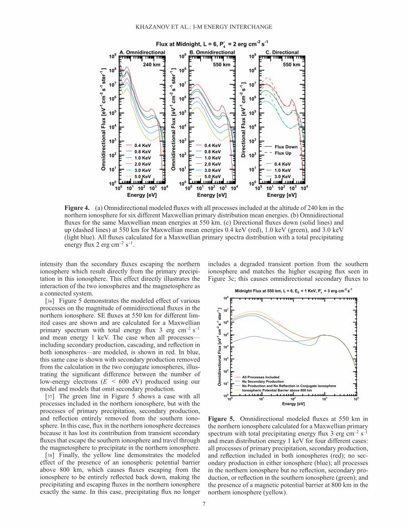
[33] Next, we illustrate the dependence of secondaryionospheric fluxes on the mean energy of the precipitat-ing primary distribution. Figure 4 displays omnidirectionaland directional SE fluxes in the northern ionosphere calcu-lated for a Maxwellian primary spectrum with a constantenergy flux of 2 erg cm–2 s–1 for all selected mean ener-gies. Figures 4a and 4b include omnidirectional fluxes at240 km and 550 km, respectively, for primary distribution

5


Figure 2. (a) Omnidirectional modeled fluxes with all processes included at altitudes of 150 km (red),240 km (purple), and 550 km (blue) in the northern ionosphere for a Gaussian primary spectrum at theinjection altitude of 800 km (black). (b) Omnidirectional fluxes for a Maxwellian primary spectrum.(c) Ratio of secondary fluxes produced by a Gaussian-to-Maxwellian distribution. All primary spectradistributions have a total precipitating energy flux of 1 erg cm–2 s–1 and mean distribution energy of 1 keV.

mean energies ranging from 0.4 keV (shown in red) to5.0 keV (yellow). With the total precipitating energy fluxheld constant, as the mean energy of the particles in theMaxwellian primary distribution increases, there are fewerparticles needed to carry the same total energy. As a result,and the peak of the distribution flattens in the energy rangeof the primary beam (E > 600 eV).

Figure 3. Omnidirectional flux in the plasmasphere (E 1–500 eV) beginning in the northern ionosphere at altitudesof 800 km to 46,000 km along the field line, calculated forsymmetric Maxwellian primary precipitation with a meandistribution energy of 0.4 keV and a total precipitatingdownward flux of 1 erg cm–2 s–1.

[34] In Figure 4, the omnidirectional secondary fluxes(E < 600 eV) at 240 km (a) and 550 km (b) maintain thesame structure at each different mean energy. However, asthe mean energy of the primary distribution increases, thesecondary fluxes also decrease in intensity by more than anorder of magnitude. This decrease is due to two processes:the decreased efficiency of secondary electron production athigher mean energies, and the increased ionospheric pen-etration depth of higher-energy particles, which makes theresultant secondary electrons less likely to escape upwardfrom the ionospheric altitudes where their mean free pathbecomes less than the scale height of the neutral atmosphere.

[35] Figure 4c includes directional fluxes down (solidlines) and up (dashed lines) at 550 km in the northern iono-sphere for three mean energies of the Maxwellian primarydistribution: 0.4 keV (red), 1.0 keV (green), and 3.0 keV(light blue). In the energy range of the primary beam (E >600 eV), fluxes down are greater than fluxes up due tothe degradation of the precipitating beam in the ionosphere.However, the secondary electron flux (E < 600 eV) escap-ing up out of the northern ionosphere is greater than theflux precipitating into the ionosphere in this energy range.As described above, we include symmetric precipitation inthe two conjugate ionospheres. In Figure 4c, we displaydirectional fluxes for the northern ionosphere, where the pre-cipitating secondary fluxes include a contribution from theparticles escaping the northern ionosphere that are backscat-tered from the plasmasphere, as well as a contribution fromthe secondary fluxes returned from the conjugate southernionosphere. These downward secondary fluxes in the north-ern ionosphere have undergone low-energy degradation dueto trapping and scattering processes during their travelthrough the plasmasphere. Consequently, they have a lower

6


Figure 4. (a) Omnidirectional modeled fluxes with all processes included at the altitude of 240 km in thenorthern ionosphere for six different Maxwellian primary distribution mean energies. (b) Omnidirectionalfluxes for the same Maxwellian mean energies at 550 km. (c) Directional fluxes down (solid lines) andup (dashed lines) at 550 km for Maxwellian mean energies 0.4 keV (red), 1.0 keV (green), and 3.0 keV(light blue). All fluxes calculated for a Maxwellian primary spectra distribution with a total precipitatingenergy flux 2 erg cm–2 s–1.

intensity than the secondary fluxes escaping the northernionosphere which result directly from the primary precipi-tation in this ionosphere. This effect directly illustrates theinteraction of the two ionospheres and the magnetosphere asa connected system.

[36] Figure 5 demonstrates the modeled effect of variousprocesses on the magnitude of omnidirectional fluxes in thenorthern ionosphere. SE fluxes at 550 km for different lim-ited cases are shown and are calculated for a Maxwellianprimary spectrum with total energy flux 3 erg cm–2 s–1

and mean energy 1 keV. The case when all processes—including secondary production, cascading, and reflection inboth ionospheres—are modeled, is shown in red. In blue,this same case is shown with secondary production removedfrom the calculation in the two conjugate ionospheres, illus-trating the significant difference between the number oflow-energy electrons (E < 600 eV) produced using ourmodel and models that omit secondary production.

[37] The green line in Figure 5 shows a case with allprocesses included in the northern ionosphere, but with theprocesses of primary precipitation, secondary production,and reflection entirely removed from the southern iono-sphere. In this case, flux in the northern ionosphere decreasesbecause it has lost its contribution from transient secondaryfluxes that escape the southern ionosphere and travel throughthe magnetosphere to precipitate in the northern ionosphere.

[38] Finally, the yellow line demonstrates the modeledeffect of the presence of an ionospheric potential barrierabove 800 km, which causes fluxes escaping from theionosphere to be entirely reflected back down, making theprecipitating and escaping fluxes in the northern ionosphereexactly the same. In this case, precipitating flux no longer

includes a degraded transient portion from the southernionosphere and matches the higher escaping flux seen inFigure 3c; this causes omnidirectional secondary fluxes to

Figure 5. Omnidirectional modeled fluxes at 550 km inthe northern ionosphere calculated for a Maxwellian primaryspectrum with total precipitating energy flux 3 erg cm–2 s–1

and mean distribution energy 1 keV for four different cases:all processes of primary precipitation, secondary production,and reflection included in both ionospheres (red); no sec-ondary production in either ionosphere (blue); all processesin the northern ionosphere but no reflection, secondary pro-duction, or reflection in the southern ionosphere (green); andthe presence of a magnetic potential barrier at 800 km in thenorthern ionosphere (yellow).

7


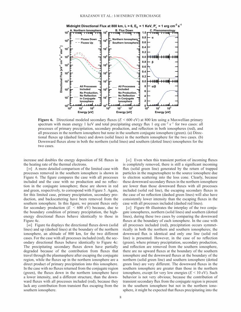
Figure 6. Directional modeled secondary fluxes (E < 600 eV) at 800 km using a Maxwellian primaryspectrum with mean energy 1 keV and total precipitating energy flux 1 erg cm–2 s–1 for two cases: allprocesses of primary precipitation, secondary production, and reflection in both ionospheres (red), andall processes in the northern ionosphere but none in the southern conjugate ionosphere (green). (a) Direc-tional fluxes up (dashed lines) and down (solid lines) in the northern ionosphere for the two cases. (b)Downward fluxes alone in both the northern (solid lines) and southern (dotted lines) ionospheres for thetwo cases.

increase and doubles the energy deposition of SE fluxes inthe heating rate of the thermal electrons.

[39] A more detailed comparison of the limited case withprocesses removed in the southern ionosphere is shown inFigure 6. The figure compares the case with all processesincluded and the case with no production and no reflec-tion in the conjugate ionosphere; these are shown in redand green, respectively, to correspond with Figure 5. Again,for this limited case, primary precipitation, secondary pro-duction, and backscattering have been removed from thesouthern ionosphere. In this figure, we present fluxes onlyfor secondary production (E < 600 eV) because, due tothe boundary condition of primary precipitation, the high-energy directional fluxes behave identically to those inFigure 4c.

[40] Figure 6a displays the directional fluxes down (solidlines) and up (dashed lines) at the boundary of the northernionosphere, an altitude of 800 km, for the two differentcases. For the case with all processes included (red), the sec-ondary directional fluxes behave identically to Figure 4c:The precipitating secondary fluxes down have partiallydegraded because of the contribution from fluxes thattravel through the plasmasphere after escaping the conjugateregion, while the fluxes up in the northern ionosphere are adirect product of primary precipitation into this ionosphere.In the case with no fluxes returned from the conjugate region(green), the fluxes down in the northern ionosphere havea lower intensity, and a different structure, than the down-ward fluxes with all processes included (red), because theylack any contribution from transient flux escaping from thesouthern ionosphere.

[41] Even when this transient portion of incoming fluxesis completely removed, there is still a significant incomingflux (solid green line) generated by the return of trappedparticles in the magnetosphere to the source ionosphere dueto electron scattering into the loss cone. Clearly, becausethese downward secondary fluxes in the northern ionosphereare lower than those downward fluxes with all processesincluded (solid red line), the escaping secondary fluxes inthe case of no reflection (dashed green lines) will also haveconsistently lower intensity than the escaping fluxes in thecase with all processes included (dashed red lines).

[42] Figure 6b illustrates the interplay of the two conju-gate ionospheres, northern (solid lines) and southern (dottedlines), during these two cases by comparing the downwardfluxes at the boundary of each ionosphere. In the case withall processes included (red), precipitation occurs symmet-rically in both the northern and southern ionospheres; thedownward flux is identical and only one line (solid redline) is presented. However, in the case of no reflection(green), where primary precipitation, secondary production,and reflection are removed from the southern ionosphere,there are no upward fluxes at the boundary of the southernionosphere and the downward fluxes at the boundary of thenorthern (solid green line) and southern ionosphere (dottedgreen line) are very different. The downward fluxes in thesouthern ionosphere are greater than those in the northernionosphere, except for very low energies (E < 10 eV). Suchbehavior is not very obvious; because the contribution oftransient secondary flux from the conjugate region is presentin the southern ionosphere but not in the northern iono-sphere, it might be expected that fluxes precipitating into the

8


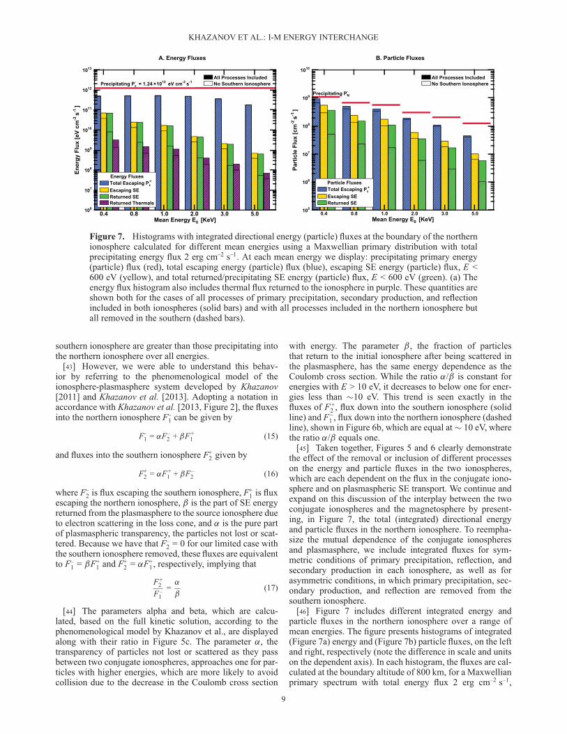
Figure 7. Histograms with integrated directional energy (particle) fluxes at the boundary of the northernionosphere calculated for different mean energies using a Maxwellian primary distribution with totalprecipitating energy flux 2 erg cm–2 s–1. At each mean energy we display: precipitating primary energy(particle) flux (red), total escaping energy (particle) flux (blue), escaping SE energy (particle) flux, E <600 eV (yellow), and total returned/precipitating SE energy (particle) flux, E < 600 eV (green). (a) Theenergy flux histogram also includes thermal flux returned to the ionosphere in purple. These quantities areshown both for the cases of all processes of primary precipitation, secondary production, and reflectionincluded in both ionospheres (solid bars) and with all processes included in the northern ionosphere butall removed in the southern (dashed bars).

southern ionosphere are greater than those precipitating intothe northern ionosphere over all energies.

[43] However, we were able to understand this behav-ior by referring to the phenomenological model of theionosphere-plasmasphere system developed by Khazanov[2011] and Khazanov et al. [2013]. Adopting a notation inaccordance with Khazanov et al. [2013, Figure 2], the fluxesinto the northern ionosphere F–

1 can be given by

F–1 = ˛F –

2 + ˇF +1 (15)

and fluxes into the southern ionosphere F+2 given by

F+2 = ˛F +

1 + ˇF –2 (16)

where F–2 is flux escaping the southern ionosphere, F+

1 is fluxescaping the northern ionosphere, ˇ is the part of SE energyreturned from the plasmasphere to the source ionosphere dueto electron scattering in the loss cone, and ˛ is the pure partof plasmaspheric transparency, the particles not lost or scat-tered. Because we have that F–

2 = 0 for our limited case withthe southern ionosphere removed, these fluxes are equivalentto F–

1 = ˇF+1 and F+

2 = ˛F+1 , respectively, implying that

F +2

F –1

=˛

ˇ(17)

[44] The parameters alpha and beta, which are calcu-lated, based on the full kinetic solution, according to thephenomenological model by Khazanov et al., are displayedalong with their ratio in Figure 5c. The parameter ˛, thetransparency of particles not lost or scattered as they passbetween two conjugate ionospheres, approaches one for par-ticles with higher energies, which are more likely to avoidcollision due to the decrease in the Coulomb cross section

with energy. The parameter ˇ, the fraction of particlesthat return to the initial ionosphere after being scattered inthe plasmasphere, has the same energy dependence as theCoulomb cross section. While the ratio ˛/ˇ is constant forenergies with E > 10 eV, it decreases to below one for ener-gies less than �10 eV. This trend is seen exactly in thefluxes of F +

2 , flux down into the southern ionosphere (solidline) and F –

1 , flux down into the northern ionosphere (dashedline), shown in Figure 6b, which are equal at � 10 eV, wherethe ratio ˛/ˇ equals one.

[45] Taken together, Figures 5 and 6 clearly demonstratethe effect of the removal or inclusion of different processeson the energy and particle fluxes in the two ionospheres,which are each dependent on the flux in the conjugate iono-sphere and on plasmaspheric SE transport. We continue andexpand on this discussion of the interplay between the twoconjugate ionospheres and the magnetosphere by present-ing, in Figure 7, the total (integrated) directional energyand particle fluxes in the northern ionosphere. To reempha-size the mutual dependence of the conjugate ionospheresand plasmasphere, we include integrated fluxes for sym-metric conditions of primary precipitation, reflection, andsecondary production in each ionosphere, as well as forasymmetric conditions, in which primary precipitation, sec-ondary production, and reflection are removed from thesouthern ionosphere.

[46] Figure 7 includes different integrated energy andparticle fluxes in the northern ionosphere over a range ofmean energies. The figure presents histograms of integrated(Figure 7a) energy and (Figure 7b) particle fluxes, on the leftand right, respectively (note the difference in scale and unitson the dependent axis). In each histogram, the fluxes are cal-culated at the boundary altitude of 800 km, for a Maxwellianprimary spectrum with total energy flux 2 erg cm–2 s–1,

9


equivalent to 1.24 � 1012 eV/cm2 s, shown as a red line inFigure 7a. Along the independent axis, both the integratedenergy and particle flux histograms display fluxes calcu-lated for a range of mean energies from 0.4 keV to 5.0 keV.While downward precipitating energy flux is constant acrossall mean energies, as shown by the red horizontal line inFigure 7a, this constant energy flux causes the precipitatingparticle flux to vary inversely as a function of mean energy,as shown by the staggered red horizontal lines representingdownward particle flux.

[47] Each histogram displays the integrated energy(Figure 7a) or particle (Figure 7b) flux of three quantities:all electrons escaping the ionosphere (blue, integrated over1 eV–10 keV), escaping SE electrons (yellow, integratedover 1–600 eV), and SE electrons returned to the iono-sphere (green, integrated over 1–600 eV). The solid colors inboth histograms represent the magnitude of fluxes when allprocesses, including secondary production, reflection fromthe conjugate ionosphere, and cascading, are modeled. Thedashed lines represent the results when all these processesare removed in the conjugate ionosphere.

[48] In the case with all processes included (solid col-ors), over mean energies 0.4 keV to 5.0 keV, the totalenergy that escapes the ionosphere (Figure 7a, blue) as apercent of precipitating energy (red) decreases from 40%to 15%. Similarly, the number of total particles that escape(Figure 7b, blue) as a percent of precipitating particles (red)decreases from 85% to 35%. Simultaneously, the escap-ing SE particles (Figure 7b, yellow) as a percent of totalescaping particle flux (Figure 7b, blue) decreases from 55%to 20%. This decrease in escaping flux with the increas-ing mean energy of the primary beam was also observed inFigures 4a and 4b. As discussed above, it is due to two pro-cesses: the decreased efficiency of the secondary electronproduction at higher mean energies and the increased iono-spheric penetration depth of high-energy particles, whichmakes their resultant secondary electrons less likely toescape upward from the ionospheric altitudes where theirmean free path becomes less than the height scale of theneutral atmosphere.

[49] Each histogram also includes these values for thecase when the conjugate ionosphere is removed completely(shown in dashed lines) and no primary beam, secondaryproduction, nor reflection occurs in the southern iono-sphere. This case corresponds to the case shown in green onFigures 5 and 6. These fluxes are significantly lower than thefluxes with all processes included, as explained above in thedescription of Figure 6a. For each mean energy, there is arelatively larger difference between the returned SE (green)and the escaping SE (yellow) energy and particle fluxeswhen the conjugate ionosphere is removed (dashed lines)than when all processes are included, also noted previouslyin the description of Figure 6a.

[50] The energy flux histogram (Figure 7a) also includesthe conductivity flux of the thermal electrons (purple), whichis defined by the following two-step integration process.First, we calculate the local heating rate along the selectedmagnetic field line, as defined by Khazanov [1979]:

Q = Ane

8<:�0(Emin) +

1ZEmin

�0(E)E

dE

9=; (18)

Figure 8. Albedo, the ratio of fluxes escaping the northernionosphere to fluxes precipitating into the northern iono-sphere, presented for different mean energies from 0.4 keV(red) to 5.0 keV (purple). Fluxes are calculated for aMaxwellian primary distribution with constant downwardprecipitating flux of 1 erg cm–2 s–1. The black line showsalbedo when cascading processes are removed in thenorthern ionosphere for a mean energy of 3.0 keV.

where �0(Emin) is omnidirectional flux at the energy of1 eV, the lowest energy of our simulation. Because thermalconductivity is the fastest process of energy loss in the plas-masphere, all energy that collects along the field tube willflow down with the energy flux at the ionospheric boundarycalculated as

Pi =siZ

s0

QBi

Bds (19)

where the i subscript indicates quantities at the ionosphericboundary and the 0 subscript is for the equatorial plane. Theintegral only covers half of the flux tube because the energydeposition is shared between the two conjugate foot pointsof the field line.

[51] This energy deposition, labeled as Returned Thermals(purple) in the histogram, range from 3 � 109eV/cm2 s to7 � 107eV/cm2 s. This returning flux is only 7%–12% of theescaping SE energy flux; the missing energy must have beentrapped in the plasmasphere.

[52] While the histograms of Figure 7 are useful to com-pare integrated quantities, they hide changes that occur as afunction of particle energy. Though we compare the ratio ofthe number of particles escaping to the number particles pre-cipitating in one ionosphere in Figure 7b, we would also liketo discuss the change in this ratio over the energy range ofprimary fluxes, 600 eV–10 keV.

[53] Following Khazanov [2011] and Khazanov et al.[2013], we define albedo as

A = F +1 /F –

1 (20)

where F +1 is flux escaping the northern ionosphere and F –

1 isflux precipitating into the northern ionosphere.

[54] Figure 8 displays this ratio for different mean ener-gies from 0.4 keV (red) to 5.0 keV (purple), calculated for a

10


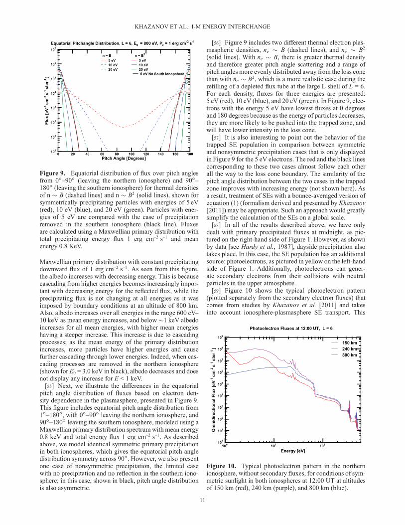
Figure 9. Equatorial distribution of flux over pitch anglesfrom 0ı–90ı (leaving the northern ionosphere) and 90ı–180ı (leaving the southern ionosphere) for thermal densitiesof n � B (dashed lines) and n � B2 (solid lines), shown forsymmetrically precipitating particles with energies of 5 eV(red), 10 eV (blue), and 20 eV (green). Particles with ener-gies of 5 eV are compared with the case of precipitationremoved in the southern ionosphere (black line). Fluxesare calculated using a Maxwellian primary distribution withtotal precipitating energy flux 1 erg cm–2 s–1 and meanenergy 0.8 KeV.

Maxwellian primary distribution with constant precipitatingdownward flux of 1 erg cm–2 s–1. As seen from this figure,the albedo increases with decreasing energy. This is becausecascading from higher energies becomes increasingly impor-tant with decreasing energy for the reflected flux, while theprecipitating flux is not changing at all energies as it wasimposed by boundary conditions at an altitude of 800 km.Also, albedo increases over all energies in the range 600 eV–10 keV as mean energy increases, and below �1 keV albedoincreases for all mean energies, with higher mean energieshaving a steeper increase. This increase is due to cascadingprocesses; as the mean energy of the primary distributionincreases, more particles have higher energies and causefurther cascading through lower energies. Indeed, when cas-cading processes are removed in the northern ionosphere(shown for E0 = 3.0 keV in black), albedo decreases and doesnot display any increase for E < 1 keV.

[55] Next, we illustrate the differences in the equatorialpitch angle distribution of fluxes based on electron den-sity dependence in the plasmasphere, presented in Figure 9.This figure includes equatorial pitch angle distribution from1ı–180ı, with 0ı–90ı leaving the northern ionosphere, and90ı–180ı leaving the southern ionosphere, modeled using aMaxwellian primary distribution spectrum with mean energy0.8 keV and total energy flux 1 erg cm–2 s–1. As describedabove, we model identical symmetric primary precipitationin both ionospheres, which gives the equatorial pitch angledistribution symmetry across 90ı. However, we also presentone case of nonsymmetric precipitation, the limited casewith no precipitation and no reflection in the southern iono-sphere; in this case, shown in black, pitch angle distributionis also asymmetric.

[56] Figure 9 includes two different thermal electron plas-maspheric densities, ne � B (dashed lines), and ne � B2

(solid lines). With ne � B, there is greater thermal densityand therefore greater pitch angle scattering and a range ofpitch angles more evenly distributed away from the loss conethan with ne � B2, which is a more realistic case during therefilling of a depleted flux tube at the large L shell of L = 6.For each density, fluxes for three energies are presented:5 eV (red), 10 eV (blue), and 20 eV (green). In Figure 9, elec-trons with the energy 5 eV have lowest fluxes at 0 degreesand 180 degrees because as the energy of particles decreases,they are more likely to be pushed into the trapped zone, andwill have lower intensity in the loss cone.

[57] It is also interesting to point out the behavior of thetrapped SE population in comparison between symmetricand nonsymmetric precipitation cases that is only displayedin Figure 9 for the 5 eV electrons. The red and the black linescorresponding to these two cases almost follow each otherall the way to the loss cone boundary. The similarity of thepitch angle distribution between the two cases in the trappedzone improves with increasing energy (not shown here). Asa result, treatment of SEs with a bounce-averaged version ofequation (1) (formalism derived and presented by Khazanov[2011]) may be appropriate. Such an approach would greatlysimplify the calculation of the SEs on a global scale.

[58] In all of the results described above, we have onlydealt with primary precipitated fluxes at midnight, as pic-tured on the right-hand side of Figure 1. However, as shownby data [see Hardy et al., 1987], dayside precipitation alsotakes place. In this case, the SE population has an additionalsource: photoelectrons, as pictured in yellow on the left-handside of Figure 1. Additionally, photoelectrons can gener-ate secondary electrons from their collisions with neutralparticles in the upper atmosphere.

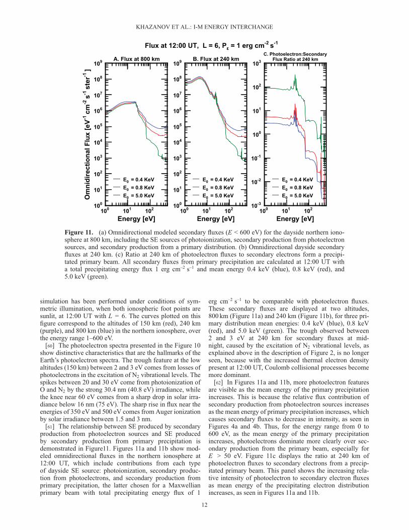
[59] Figure 10 shows the typical photoelectron pattern(plotted separately from the secondary electron fluxes) thatcomes from studies by Khazanov et al. [2011] and takesinto account ionosphere-plasmasphere SE transport. This

Figure 10. Typical photoelectron pattern in the northernionosphere, without secondary fluxes, for conditions of sym-metric sunlight in both ionospheres at 12:00 UT at altitudesof 150 km (red), 240 km (purple), and 800 km (blue).

11


Figure 11. (a) Omnidirectional modeled secondary fluxes (E < 600 eV) for the dayside northern iono-sphere at 800 km, including the SE sources of photoionization, secondary production from photoelectronsources, and secondary production from a primary distribution. (b) Omnidirectional dayside secondaryfluxes at 240 km. (c) Ratio at 240 km of photoelectron fluxes to secondary electrons form a precipi-tated primary beam. All secondary fluxes from primary precipitation are calculated at 12:00 UT witha total precipitating energy flux 1 erg cm–2 s–1 and mean energy 0.4 keV (blue), 0.8 keV (red), and5.0 keV (green).

simulation has been performed under conditions of sym-metric illumination, when both ionospheric foot points aresunlit, at 12:00 UT with L = 6. The curves plotted on thisfigure correspond to the altitudes of 150 km (red), 240 km(purple), and 800 km (blue) in the northern ionosphere, overthe energy range 1–600 eV.

[60] The photoelectron spectra presented in the Figure 10show distinctive characteristics that are the hallmarks of theEarth’s photoelectron spectra. The trough feature at the lowaltitudes (150 km) between 2 and 3 eV comes from losses ofphotoelectrons in the excitation of N2 vibrational levels. Thespikes between 20 and 30 eV come from photoionization ofO and N2 by the strong 30.4 nm (40.8 eV) irradiance, whilethe knee near 60 eV comes from a sharp drop in solar irra-diance below 16 nm (75 eV). The sharp rise in flux near theenergies of 350 eV and 500 eV comes from Auger ionizationby solar irradiance between 1.5 and 3 nm.

[61] The relationship between SE produced by secondaryproduction from photoelectron sources and SE producedby secondary production from primary precipitation isdemonstrated in Figure11. Figures 11a and 11b show mod-eled omnidirectional fluxes in the northern ionosphere at12:00 UT, which include contributions from each typeof dayside SE source: photoionization, secondary produc-tion from photoelectrons, and secondary production fromprimary precipitation, the latter chosen for a Maxwellianprimary beam with total precipitating energy flux of 1

erg cm–2 s–1 to be comparable with photoelectron fluxes.These secondary fluxes are displayed at two altitudes,800 km (Figure 11a) and 240 km (Figure 11b), for three pri-mary distribution mean energies: 0.4 keV (blue), 0.8 keV(red), and 5.0 keV (green). The trough observed between2 and 3 eV at 240 km for secondary fluxes at mid-night, caused by the excitation of N2 vibrational levels, asexplained above in the description of Figure 2, is no longerseen, because with the increased thermal electron densitypresent at 12:00 UT, Coulomb collisional processes becomemore dominant.

[62] In Figures 11a and 11b, more photoelectron featuresare visible as the mean energy of the primary precipitationincreases. This is because the relative flux contribution ofsecondary production from photoelectron sources increasesas the mean energy of primary precipitation increases, whichcauses secondary fluxes to decrease in intensity, as seen inFigures 4a and 4b. Thus, for the energy range from 0 to600 eV, as the mean energy of the primary precipitationincreases, photoelectrons dominate more clearly over sec-ondary production from the primary beam, especially forE > 50 eV. Figure 11c displays the ratio at 240 km ofphotoelectron fluxes to secondary electrons from a precip-itated primary beam. This panel shows the increasing rela-tive intensity of photoelectron to secondary electron fluxesas mean energy of the precipitating electron distributionincreases, as seen in Figures 11a and 11b.

12


5. Summary and Conclusion

[63] Diffuse auroral precipitation covers a broad rangeof geomagnetic latitudes, which map along field lines fromthe inner magnetosphere to the plasma sheet. Diffuse pre-cipitation of energetic electrons from the magnetosphere isa consequence of pitch angle scattering by different kindsof plasma waves. The precipitation of energetic electronsin the diffuse auroral region is an important source of ion-izing energy input to the middle atmosphere and heatingof the thermal plasma. The dissipation process of magne-tospheric electrons in the diffuse aurora is also affiliatedwith the cascading of higher-energy electrons toward ther-mal energies and the production of secondary electrons.This lower energy electron population can escape back tothe magnetosphere and become trapped on closed magneticfield lines. In this paper, for the first time, we discussedmagnetosphere-ionosphere-atmosphere coupling collisionalprocesses in the electron diffuse aurora, focusing on theenergy and particle interplay between the two magneticallyconjugate ionospheres and outer plasmasphere.

[64] We found quantitative relations between the energyand particle fluxes that precipitate from the magnetosphereinto the ionosphere and the affiliated secondary electron pop-ulation escaping back to the magnetosphere (Figures 4–7).The SEs that travel to the magnetosphere can be trappedby the Earth’s magnetic field and deliver a portion of theirenergy to the thermal electrons of the outer plasmasphere(Figure 7). This energy, however, does not stay in the magne-tosphere, because thermal conductivity is the fastest processof the energy loss in the plasmasphere and all of the energythat was collected along the field tube will flow down to theionosphere, contributing to the ionospheric energy balancebetween thermal electrons and ions.

[65] As we have demonstrated, there is a very complicatedenergy interplay between the two magnetically conjugatedionospheres and the outer plasmasphere. Our quantitativeanalysis has been made in order to address this issue bystudying different limited cases when one of the conjugatedionospheres was completely or partially separated from suchenergy, an exchange between the plasmasphere and anotherionosphere (Figures 5–7). We have also seen that the meanenergy of the precipitating diffuse auroral electrons has asignificant effect on the relative role of secondary flux inten-sity, cascading (Figure 8), and photoelectron production onthe dayside (Figure 11).

[66] As we pointed out in the introduction to our paper,the diffuse aurora, which is always present and widelydistributed in rings around Earth’s magnetic poles, col-lectively accounts for about three-quarters of the auroralenergy precipitating into the ionosphere [e.g., Newell et al.,2009]. For this reason, as demonstrated by the quantita-tive analysis presented in this paper, diffuse auroral pre-cipitation must be included in the development of globalmodels by taking into account ionosphere-magnetosphereenergy interplay between precipitated high-energy electronsof magnetospheric origin, the resultant secondary electronpopulation escaping back to the magnetosphere, its trap-ping in this region, and its heating of the thermal populationof the outer plasmasphere, with the consequent thermalconductivity flux formation that returns back to the upperionosphere. Neglecting any of these processes will yield anincomplete picture.

[67] Acknowledgments. This material is based upon work supportedby the National Aeronautics and Space Administration SMD/HeliophysicsSupporting Research and Living With a Star programs for Geospace SR&T.

[68] Robert Lysak thanks the reviewers for their assistance in evaluatingthis paper.

ReferencesArnoldy, R. L., P. O. Isaacson, and P. B. Lewis (1974), Field-

aligned auroral electron fluxes, J. Geophys. Res., 79, 4208–4221,doi:10.1029/JA079i028p04208.

Banks, P. M., C. R. Chappell, and A. F. Nagy (1974), A new model for theinteraction of auroral electrons with the atmosphere: Spectral degrada-tion, backscatter, optical emission, and ionization, J. Geophys. Res., 79,1459–1470, doi:10.1029/JA079i010p01459.

Bell, K. L., and R. P. Stafford (1992), Photoionization cross-sections foratomic oxygen, Planet. Space Sci., 40, 1419–1424, doi:10.1016/0032-0633(92)90097-8.

Bilitza, D. (1990), Progress report on IRI status, Adv. Space Res., 10, 3–5,doi:10.1016/0273-1177(90)90298-E.

Conway, R. (1988), Photoabsorption and Photoionization Cross Sections:A Compilation of Recent Measurements, NRL Memo Rep. 6155, NavalResearch Laboratory, Washington, D. C.

Eather, R. H., and S. B. Mende (1971), Airborne observations ofauroral precipitation patterns, J. Geophys. Res., 76, 1746–1755,doi:10.1029/JA076i007p01746.

Ebihara, Y., T. Sakanoi, K. Asamura, M. Hirahara, and M. F. Thomsen(2010), Reimei observation of highly structured auroras caused bynonaccelerated electrons, J. Geophys. Res., 115, A08320, doi:10.1029/2009JA015009.

Evans, D. S. (1974), Precipitating electron fluxes formed by a magneticfield aligned potential difference, J. Geophys. Res., 79, 2853–2858,doi:10.1029/JA079i019p02853.

Fennelly, J. A., and D. G. Torr (1992), Photoionization and PhotoabsorptionCross Sections of O, N2 O2, and N for Aeronomic Calculations, Atom.Data Nucl. Data Tables, 51, 321, doi:10.1016/0092-640X(92)90004-2.

Fontaine, D., and M. Blanc (1983), A theoretical approach to the morphol-ogy and the dynamics of diffuse auroral zones, J. Geophys. Res., 88,7171–7184, doi:10.1029/JA088iA09p07171.

Frank, L. A., and K. L. Ackerson (1971), Observations of charged parti-cle precipitation into the auroral zone, J. Geophys. Res., 76, 3612–3643,doi:10.1029/JA076i016p03612.

Hardy, D., M. Gussenhoven, R. Raistrick, and W. McNeil (1987), Statisticaland fuctional representation of the pattern of auroral energy flux, numberflux, and conductivity, J. Geophys. Res., 92, 12,275–12,294.

Hedin, A. (1991), Extension of the MSIS thermosphere model into themiddle and lower atmosphere, J. Geophys. Res., 96, 1159–1172.

Hinteregger, H., K. Fukui, and B. Gibson (1981), Observational, referenceand model data on solar EUV from measurements on AE-E, Geophys.Res. Lett., 8, 1147–1150.

Hoffman, R. A., and J. L. Burch (1973), Electron precipitation pat-terns and substorm morphology, J. Geophys. Res., 78, 2867–2884,doi:10.1029/JA078i016p02867.

Johnstone, A. D., D. M. Walton, R. Liu, and D. A. Hardy (1993), Pitch anglediffusion of low-energy electrons by whistler mode waves, J. Geophys.Res., 98, 5959–5967, doi:10.1029/92JA02376.

Kennel, C. F., and H. E. Petschek (1966), Limit on stably trapped particlefluxes, J. Geophys. Res., 71, 1–28.

Khazanov, G. (1979), The Kinetics of the Electron Plasma Componentof the Upper Atmosphere, Nauka, Moscow, [English translation: #80-50707, National Translation Center, Washington, D. C. 1980].

Khazanov, G. (2011), Kinetic Theory of the Inner Magnetospheric Plasma,Astrophysics and Space Science Library, Springer.

Khazanov, G., M. W. Liemohn, T. I. Gombosi, and A. F. Nagy (1993),Non-steady-state transport of superthermal electrons in the plasmasphere,Geophys. Res. Lett., 20, 2821–2824.

Khazanov, G. V., M. A. Koen, I. V. Konikov, and I. M. Sidorov (1984),Simulation of ionosphere-plasmasphere coupling taking into account ioninertia and temperature anisotropy, Planet. Space Sci., 32, 585–598,doi:10.1016/0032-0633(84)90108-9.

Khazanov, G. V., T. Neubert, and G. D. Gefan (1994), Unified theory ofionosphere-plasmasphere transport of suprathermal electrons, IEEE T.Plasma Sci., 22, 187–198, doi:10.1109/27.279022.

Khazanov, G. V., M. W. Liemohn, T. S. Newman, M.-C. Fok, and R. W.Spiro (2003), Self-consistent magnetosphere-ionosphere coupling: Theo-retical studies, J. Geophys. Res., 108, 1122, doi:10.1029/2002JA009624.

Khazanov, G. V., D. E. Rowland, T. E. Moore, and M. R. Collier (2011),The VISIONS Science, Abstract SM31A-2087 presented at 2011 FallMeeting, AGU, San Francisco, Calif.

13


Khazanov, G. V., A. Glocer, M. W. Liemohn, and E. W. Himwich(2013), Superthermal electron energy interchange in the ionosphere-plasmasphere system, J. Geophys. Res. Space Physics, 118, 925–934,doi:10.1002/jgra.50127.

Link, R. (1992), Feautrier solution of the electron transport equation,J. Geophys. Res., 97, 159–169, doi:10.1029/91JA02214.

Lui, A. T. Y., and C. D. Anger (1973), A uniform belt of diffuse auroralemission seen by the ISIS-2 scanning photometer, Planet. Space Sci., 21,799–799, doi:10.1016/0032-0633(73)90097-4.

Lui, A. T. Y., S.-I. Akasofu, D. Venkatesan, C. D. Anger, W. J. Heikkila,J. D. Winningham, and J. R. Burrows (1977), Simultaneous obser-vations of particle precipitations and auroral emissions by the Isis 2satellite in the 19-24 MLT sector, J. Geophys. Res., 82, 2210–2226,doi:10.1029/JA082i016p02210.

Lummerzheim, D., and J. Lilensten (1994), Electron transport andenergy degradation in the ionosphere: Evaluation of the numeri-cal solution, comparison with laboratory experiments and auroralobservations, Ann. Geophys., 12, 1039–1051, doi:10.1007/s00585-994-1039-7.

Lyons, L. R. (1974), Pitch angle and energy diffusion coefficients from reso-nant interactions with ion-cyclotron and whistler waves, J. Plasma Phys.,12, 417–432, doi:10.1017/S002237780002537X.

Meng, C.-I., B. Mauk, and C. E. McIlwain (1979), Electron precip-itation of evening diffuse aurora and its conjugate electron fluxesnear the magnetospheric equator, J. Geophys. Res., 84, 2545–2558,doi:10.1029/JA084iA06p02545.

Min, Q.-L., D. Lummerzheim, M. H. Rees, and K. Stamnes (1993), Effectsof a parallel electric field and the geomagnetic field in the topside iono-sphere on auroral and photoelectron energy distributions, J. Geophys.Res., 98, 19,223–19,234, doi:10.1029/93JA01742.

Mishin, E. V., A. A. Trukhan, and G. V. Khazanov (1990), Plasma effectsof superthermal electrons in the ionosphere, Nauka, Moscow.

Newell, P. T., T. Sotirelis, and S. Wing (2009), Diffuse, monoenergetic, andbroadband aurora: The global precipitation budget, J. Geophys. Res., 114,A09207, doi:10.1029/2009JA014326.

Newell, P. T., A. R. Lee, K. Liou, S.-I. Ohtani, T. Sotirelis, and S.Wing (2010), Substorm cycle dependence of various types of aurora,J. Geophys. Res., 115, A09226, doi:10.1029/2010JA015331.

Nishimura, Y., et al. (2013), Structures of dayside whistler-mode wavesdeduced from conjugate diffuse aurora, J. Geophys. Res. Space Physics,118, 664–673, doi:10.1029/2012JA018242.

Peticolas, L., and D. Lummerzheim (2000), Time-dependent transport offield-aligned bursts of electrons in flickering aurora, J. Geophys. Res.,105, 12,895–12,906, doi:10.1029/1999JA000398.

Rees, D. (1989), Physics and Chemistry of the Upper Atmosphere,Cambridge Univ. Press, New York, NY.

Schumaker, T. L., R. L. Carovillano, M. S. Gussenhoven, and D. A.Hardy (1989), The relationship between diffuse auroral and plasmasheet electron distributions near local midnight, J. Geophys. Res., 94,10,061–10,078, doi:10.1029/JA094iA08p10061.

Solomon, S., P. Hays, and V. Abreu (1988), The auroral 6300Å emission:Observations and modeling, J. Geophys. Res., 93, 9867–9882.

Solomon, S. C. (1993), Auroral electron transport using the Monte Carlomethod, Geophys. Res. Lett., 20, 185–188, doi:10.1029/93GL00081.

Stamnes, K. (1981), On the two-stream approach to electron transportand thermalization, J. Geophys. Res., 86, 2405–2410, doi:10.1029/JA086iA04p02405.

Strickland, D. J., D. L. Book, T. P. Coffey, and J. A. Fedder (1976),Transport equation techniques for the deposition of auroral electrons,J. Geophys. Res., 81, 2755–2764, doi:10.1029/JA081i016p02755.

Winningham, J. D., W. J. Heikkila, F. Yasuhara, and S.-I. Akasofu (1975),The latitudinal morphology of 10-eV to 10-keV electron fluxes duringmagnetically quiet and disturbed times in the 2100-0300 MLT sector,J. Geophys. Res., 80, 3148–3171, doi:10.1029/JA080i022p03148.

14

Documents

Magnetosphereionosphere energy interchange in … energy interchange in the electron diffuse ... energy interchange in the electron diffuse aurora, J ... spirals, are pitch angle