Magnetic Resonance Studies of

Transport and Reaction in Vortical Flow

by

Antoine Vallatos

A thesis submitted to The University of Birmingham

For the degree of DOCTOR OF PHILOSOPHY

School of Chemistry College of Engineering and Physical Sciences

The University of Birmingham October 2013

University of Birmingham Research Archive

e-theses repository This unpublished thesis/dissertation is copyright of the author and/or third parties. The intellectual property rights of the author or third parties in respect of this work are as defined by The Copyright Designs and Patents Act 1988 or as modified by any successor legislation. Any use made of information contained in this thesis/dissertation must be in accordance with that legislation and must be properly acknowledged. Further distribution or reproduction in any format is prohibited without the permission of the copyright holder.

Abstract

This thesis explores the coupling of autocatalytic reactions, such as the oscillating Belousov-

Zhabotinsky reaction, with vortical flows produced in a Couette cell. Similarly to many

Reaction-Diffusion-Advection (RDA) systems found in nature, the resulting systems are

characterised by chemical cycles maintained out of equilibrium by transport processes

involving complex flow properties, such as periodicity and vorticity. In this project, an

integrated approach was developed, combining optical and magnetic resonance techniques

with modelling, to study transport and reaction in vortical flows.

Flow structure and molecular displacements within stationary and translating vortices were

investigated using a combination of magnetic resonance (MR) velocity and diffusion mapping

with MR propagator experiments. A model based on MR experimental data was developed to

simulate molecular displacements and provide quantitative information on micro-mixing and

long time-scale axial dispersion. Simulations of molecular displacements allow linkage of

molecular transport with the propagation of chemical waves travelling through vortical flows.

The macroscopic patterns arising from these RDA systems, in combination with modelling

results, allowed understanding coupling mechanisms between flow and chemistry and

characterising inter- and intra- vortex mixing. Finally, MR imaging of chemical waves was

shown to compare well with molecular displacement simulations, providing with a means for

characterising the interplay of flow and chemistry in reactive flow systems.

With love to my three beautiful families

Acknowledgments

Time and space appeared as the unbreakable constraints to the holistic acknowledgment

approach I would have liked: pages and pages acknowledging every single human interaction

that through these years helped me make small steps in the little odyssey that ended with the

book you hold in your hands. Inevitably, before focusing on the beautiful people that had

major contributions to this work, I owe some sincere excuses to those that will not see their

name in the following pages. From the bottom of my heart and soul, I would like to thank:

• My supervisor and research companion over these years, the explosive Dr. Melanie M.

Britton, for accepting me in her group, for teaching me, for believing in me and for

challenging me enough to make me feel that I deserve to be called a doctor.

• My research group, past and present: Dr. Jan Novak, for setting the grounds of my

research and transmitting me his precious knowledge (including slang). Rhys Evans for

tolerating my obsessive supervision and producing some wonderful pattern formation

data. Dr. Heather Rose, for taking care of me when I joined the team and making sure that

I do not kill myself in the lab. Sue Law for following her dreams: love, passion, pain,

science and rock’n’roll. Amanda Mills, for helping me understand all these little magnetic

things. Matt Berwick, for his funky T-shirts and swirly peptides. Ismailla Abdullahi, for

keeping the smile alive. Catherine Smith, for rocking the bars of Cambridge with me.

• My collaborators: Dr. Annette F. Taylor and Dr. Mark C.T. Wilson, for our intense and

productive meetings that lead to the publications that arouse from this work.

• My examiners: Dr. Andy Sederman and Prof. David Parker, for reading this text,

providing me with a challenging but extremely instructing viva and with corrections that

raised the level of this work. Dr. Josephine Bunch and Prof. Roy L. Johnston for reading

my first year report.

• The School of Chemistry students, academic and admin staff for being the womb of my

scientific and, to many extents, personal development over the past years.

• My friends and colleagues that patiently helped me grasp the richness of chemistry,

physics, life and beyond; by our uncountable discussions, our psychedelic events and

techno-deliria; by our lab weekends and smoking-corner meetings. For these four

beautiful years, I’d like to thank alphabetical order some of my research and life

companions: Rhapsodic Alex (mix the drinks, mix the feelings and white bottom), Andrea

the great (learn faster than Rosetta Stone can teach), Funky Stro (join the smooth psycho-

somatic ecstasy), Comrade Ben (it won’t be televised), Sublime Claire (on the road

again), Carlotta la Pasionaria (think with the heart, love with the brain), Prodigious Chris

(evolution through diffusion, order through chaos), Cristina la sirena (do the loco motion),

Manu the iconoclast (stay on 51 and fulminate the thinking machine), Bursting Marie

(organic brain and black metallic vain), Prolific Mark (do it better than Steve Jobs),

Mesmerising Michel (deep in the Steppenwolf forest), Redskin Pete (reality asylum and

white riot), Satanic Peter (I just want to say hi to my Peter, OK? Yo Peter, it’s me,

Rocky!), the eruptive Ornella (storm and fire) and Sweet Susana (my goodness gracious).

• My wonderful family, for teaching me that unity is compatible with diversity and love is

compatible with critical thinking: My parents, Smaragdi, Juan, Irini, Manu, Giorgos,

Sophie, Stephane and Joe.

• My little Amazon princess, Myrto, for everything. In particular, for convincing me to start

a PhD, for supporting stoically my research related psycho-instabilities, for helping me

understand the research environment, for financing the writing up period of this PhD, for

proof checking my manuscript, for the wonderful present she offered me for my

submission and for helping me become who I am.

Contents

1 Introduction.................................................................................................1

1.1 Prologue.......................................................................................................... 1

1.2 Thesis outline .................................................................................................. 4

1.3 Autocatalysis and oscillating chemistry ........................................................... 5

1.3.1 From autocatalysis and feedback to clocks and fronts......................................... 5

1.3.2 The BZ oscillating reaction ................................................................................ 6

1.3.3 Oscillatory system studies .................................................................................11

1.4 Flow properties of chemical reactors ............................................................. 14

1.4.1 Introduction to Newtonian laminar flow properties............................................14

1.4.2 Packed-Bed Reactors (PBRs) ............................................................................21

1.4.3 Continuous Stirred Tank Reactors (CSTRs) ......................................................23

1.4.4 Stationary vortices in a Couette cell...................................................................25

1.4.5 Travelling vortices in a Couette cell ..................................................................29

1.5 Flow distributed chemical structures ............................................................. 35

1.5.1 Chemical waves ................................................................................................35

1.5.2 Introduction to flow distributed chemical patterns .............................................40

1.5.3 Flow Distributed Oscillations (FDOs) ...............................................................46

1.5.4 The general case of flow distributed structures and its applications....................55

2 Magnetic resonance techniques ................................................................ 64

2.1 Magnetic resonance principles....................................................................... 64

2.2 Magnetic resonance relaxation ...................................................................... 67

2.2.1 T1 relaxation......................................................................................................67

2.2.2 T2 relaxation......................................................................................................69

2.3 Magnetic Resonance Imaging (MRI)............................................................. 71

2.3.1 Using magnetic gradients for spatial encoding...................................................71

2.3.2 k-space ..............................................................................................................73

2.3.3 Slice selection ...................................................................................................75

2.3.4 Spin echo imaging.............................................................................................76

2.3.5 MRI contrast .....................................................................................................78

2.4 Measurement of molecular motion ................................................................ 79

2.4.1 Pulsed gradient spin echo principles ..................................................................79

2.4.2 PGSE and PGSTE.............................................................................................84

2.4.3 Magnetic resonance imaging of velocity, diffusion and dispersion.....................85

3 MR characterisation of stationary vortex flow........................................ 89

3.1 Introduction................................................................................................... 89

3.2 Experimental ................................................................................................. 90

3.2.1 Couette cell dimensions and set-up....................................................................90

3.2.2 Parameter ranges...............................................................................................91

3.2.3 Velocity and dispersion imaging .......................................................................92

3.2.4 Propagator measurements..................................................................................93

3.3 Results and discussion................................................................................... 94

3.3.1 TVF velocity and dispersion imaging ................................................................94

3.3.2 The effect of rotation on TVF flow structure .....................................................99

3.3.3 Molecular displacements and mixing in TVF ..................................................106

3.4 Conclusions..................................................................................................110

4 MR characterisation of translating vortex flow .................................... 113

4.1 Introduction..................................................................................................113

4.2 Experimental ................................................................................................117

4.2.1 Vortex Flow Reactor dimensions and set-up....................................................117

4.2.2 Parameter ranges.............................................................................................118

4.2.3 Optical and timing measurements....................................................................119

4.2.4 Velocity imaging of steady flow......................................................................120

4.2.5 Velocity imaging of periodic flow...................................................................120

4.2.6 Propagator measurements................................................................................121

4.3 Results and discussion..................................................................................122

4.3.1 Optical visualisation of travelling vortices.......................................................122

4.3.2 Pipe flow properties ........................................................................................125

4.3.3 Velocity drift...................................................................................................127

4.3.4 MR Velocity imaging of travelling vortices.....................................................129

4.3.5 VFR flow as a superposition between pipe flow and TVF ...............................134

4.3.6 Molecular displacements and mixing...............................................................138

4.3.7 Flow and rotation rate effect on molecular displacements................................141

4.4 Conclusions..................................................................................................146

5 Molecular displacement simulations using MR data ............................ 150

5.1 Introduction..................................................................................................150

5.2 Experimental ................................................................................................152

5.2.1 Molecular displacement simulations................................................................152

5.2.2 Chemical front propagation in vortical flow ....................................................155

5.3 Results and discussion..................................................................................157

5.3.1 Molecular displacements and propagator simulations ......................................157

5.3.2 Long time scale displacements and axial dispersion.........................................160

5.3.3 Molecular paths in pipe flow ...........................................................................162

5.3.4 Molecular paths in TVF ..................................................................................164

5.3.5 Molecular paths in VFR flow ..........................................................................166

5.3.6 Chemical wave propagation in TVF ................................................................170

5.3.7 Chemical wave propagation in VFR flow........................................................172

5.4 Conclusions..................................................................................................175

6 Chemical patterns in translating vortices: intra- and inter-vortex mixing

effects ............................................................................................................ 178

6.1 Introduction..................................................................................................178

6.2 Experimental ................................................................................................181

6.2.1 The ferroin-catalysed BZ reaction ...................................................................181

6.2.2 Pt-electrode measurements of BZ temporal oscillations...................................181

6.2.3 Experimental set-up for chemical patterns in a VFR........................................182

6.2.4 Optical measurements of chemical patterns .....................................................183

6.2.5 Parameter ranges.............................................................................................184

6.2.6 Modelling chemical pattern formation in travelling vortices ............................184

6.3 Results and discussion..................................................................................187

6.3.1 Temporal oscillations in the BZ reaction .........................................................187

6.3.2 Chemical patterns in a high inter-vortex exchange system ...............................188

6.3.3 Chemical patterns in a low inter-vortex exchange system ................................197

6.3.4 Inter- and intra-vortex mixing effects ..............................................................202

6.4 Conclusions..................................................................................................206

7 MR Imaging of chemical waves in vortical flow.................................... 211

7.1 Introduction..................................................................................................211

7.2 Experimental ................................................................................................213

7.2.1 The manganese-catalysed BZ reaction.............................................................213

7.2.2 Pt-electrode measurements of BZ temporal oscillations...................................214

7.2.3 Experimental set-up for chemical waves in vortical flow.................................214

7.2.4 Flow parameter ranges ....................................................................................215

7.2.5 Optical measurements .....................................................................................215

7.2.6 T1 and T2 relaxation measurements..................................................................216

7.2.7 Relaxation-weighted imaging..........................................................................217

7.3 Results and discussion..................................................................................219

7.3.1 Optical imaging of chemical patterns in translating vortices ............................219

7.3.2 Chemistry-induced MR contrast ......................................................................225

7.3.3 Flow-induced MR contrast ..............................................................................230

7.3.4 MRI of chemical waves in stationary vortices .................................................237

7.3.5 MRI of travelling chemical waves in translating vortices.................................245

7.3.6 MR Imaging of Mn-catalysed BZ FDOs..........................................................249

7.4 Conclusions..................................................................................................251

8 Conclusions and future work.................................................................. 254

Appendix A................................................................................................... 258

Appendix B .................................................................................................. 260

Appendix C .................................................................................................. 267

Appendix D .................................................................................................. 268

List of Figures .............................................................................................. 270

Abbreviations .............................................................................................. 278

Introduction

1

1 Introduction

1.1 Prologue

Understanding the coupling between chemical reactions and transport processes is crucial in a

wide variety of disciplines as biology, chemical engineering and atmospheric science. This

coupling is ubiquitous in nature and can give rise to pattern formations both at the

microscopic and macroscopic length scales, generating phenomena as diverse as the

movement of cellular contents1 (streaming) or the growth of plankton colonies2 (blooming) in

oceanic currents. Many of these systems are characterised by the presence of non-linear

autocatalytic chemical cycles, maintained out of equilibrium by the supply of new reactants.

The transport processes that are mobilised to ensure this supply of matter, often involve the

flow properties of three-dimensionality, periodicity, vorticity and anisotropic diffusion. The

complexity of the resulting systems tends to restrict their analysis to specific field approaches

(e.g. fluid mechanics, physical chemistry), and the multitude of influencing parameters

introduces difficulties in bringing together experimental and theoretical results.

This thesis has taken an integrated approach, combining optical and magnetic resonance

(MR) techniques with modelling, to study the coupling between transport and reaction in

vortical flows. Particular attention is given to pattern formation arising from the combination

of the oscillating Belousov-Zhabotinsky (BZ) reaction with translating vortical flow in a

Couette cell. As for the biological processes mentioned earlier, maintaining the system far

from equilibrium is achieved by sustaining a flux of matter and energy. Molecular processes

taking place in such systems can lead to macroscopic patterns many orders of magnitude

Introduction

2

greater than the molecular scale.

The BZ reaction is the most famous example of an autocatalytic reaction exhibiting temporal

oscillations3−5. Since its discovery, several studies have been conducted to understand its

ability to self-organise. Because of its oscillatory behaviour, the BZ reaction is known to

produce travelling chemical waves that are spatially distributed through transport processes as

diffusion and advection. The resulting reaction-diffusion (RD) or reaction-diffusion-advection

(RDA) systems have been very studied because, under certain conditions, they give rise to

very particular pattern formation phenomena, as stationary chemical waves.

Taylor vortices are produced in the annulus between a rotating inner cylinder and a fixed

outer cylinder of a Couette cell. Above a critical rotation rate of the inner cylinder, the flow

reorganises in a series of counter rotating vortices stacked along the length of the cell6. Taylor

Vortex Flow (TVF) has been the object of numerous publications7. The addition of axial pipe

flow to TVF was shown to cause a translation of the vortices, producing a vortex flow reactor

(VFR). At certain regimes, flow in a VFR exhibits plug-like properties that are of particular

interest to several applications in various fields such as chemical engineering8 or

biochemistry9.

Most of experimental pattern formation studies using the BZ reaction and involving flow have

been done in two-dimensions using optical imaging techniques10. Similarly most of the

existing studies on the flow properties within a Couette cell have used optical techniques like

Particule Imaging Velocimetry (PIV)11 or dye visualisation12. Optical techniques present

limitations in addressing microscopic properties as they necessitate the introduction of tracers

Introduction

3

that can perturb the system. The ability of MR techniques to probe, non-invasively, both

chemical patterns and flow properties13 makes them ideally suited for studying the interplay

of chemistry and flow within these fragile systems. This project has focussed on developing

both the techniques and the methodology that enable the systematic study of the coupling

between chemistry and flow using magnetic resonance.

The combination of flow and chemistry can lead to complex behaviour of the system,

producing data that are not easy to analyse. To deal with this, an analytic approach was used

to produce models that reduce the amount of data to handle, in order to obtain accessible

qualitative and quantitative information. This approach has necessitated the definition of the

appropriate levels of description4,14 that allow identifying correlations between various

parameters:

• A molecular level where individual molecules and collisions are considered.

Depending on Arrhenius parameters, a percentage of these collisions lead to reactions.

At this level, temperature and diffusion set a common ground between chemistry and

molecular transport possesses.

• A microscopic level that deals with volume elements that are big enough to define

densities of molecules at different phases (chemical concentrations) and average

velocity or diffusion/dispersion (flow properties). At any given time, and for each

volume element, inlets and outlets can be defined by flow properties and chemical

state can be defined by concentration of different species.

• A macroscopic level, where vortices can be presented as elementary units of vortical

flow systems and pattern-forming systems can be studied as entities that arise through

the inseparable coupling between flow and chemistry.

Introduction

4

Throughout this project, one or more of these levels of description have been employed. It

should be stressed that, for a same system, the information provided at each description level

is not equivalent. One can notice that the macroscopic pattern formation arising from the

combination of flow and chemistry provides with properties that are not existent at the

molecular level.

1.2 Thesis outline

This study draws upon previous research conducted across a diverse range of scientific

disciplines: non-linear chemistry, fluid mechanics, fluid/chemistry coupling and NMR/MRI

techniques. The first part of this presentation (Chapter 1) will set the background for the flow

and chemistry coupling studies that will follow, while trying to make the necessary links with

the field of magnetic resonance (MR). This background review will introduce both

autocatalytic oscillating reactions and flow properties in chemical reactors, before presenting

the flow distributed chemical structures that arise from the combination of flow and

chemistry. Chapter 2 introduces the MR techniques that are encountered in this thesis. The

first experimental chapter (Chapter 3) presents MR studies, combining velocity and

dispersion mapping with measurements of molecular displacements, for the characterisation

of stationary vortex flow. The next chapter (Chapter 4) expands these studies to translating

vortex flow. In chapter 5, simulations of molecular displacements using MR experimental

results are performed in order to allow the prediction of axial dispersion and molecular paths

in stationary and travelling vortex flows. Results presented in chapters 3 to 5 have been

published in Europhysics letters15 (Appendix C). Chapter 6 introduces oscillating chemical

reactions and examines the macroscopic patterns formed by the combination of chemistry and

Introduction

5

travelling vortices (Flow Distributed Oscillations). Results presented in this chapter have been

published in Chaos16 (Appendix D). The last part of this thesis focuses on MR studies of the

coupling between oscillating autocatalytic chemistry and vortical flow (Chapter 7). This

presentation ends with an overview of the results and questions that arose throughout this

project and a discussion on future research possibilities (Chapter 8).

1.3 Autocatalysis and oscillating chemistry

1.3.1 From autocatalysis and feedback to clocks and fronts

A chemical reaction is said to be autocatalytic, if the reaction product is also a catalyst for the

reaction17. An example of this is a reaction where

!

A + B" 2B, with B being the autocatalytic

species. In this model scheme, the rate r of the reaction is of the form

!

r = k[A][B], showing

that an increase in [B] produces a rate increase.

Typically, such model schemes are composed of several elementary steps, and feedback arises

when the products of the later steps influence the rate of some of the earlier steps, and, hence,

the rate of their own production. This may take the form of either positive feedback (self-

acceleration) or negative feedback (self-inhibition), and result in rapid changes in the

concentration of intermediate species. If the colour of these species is visible and the reactants

well stirred, this acceleration can lead to a sharp colour change of the entire solution. Where

only a single positive feedback process is present, the result is a clock reaction characterised

by an induction time before the observation of the rapid concentration change. This is due to

the fact that the autocatalytic species needs to attain a sufficient concentration for the

Introduction

6

autocatalytic step to be initiated. Other elementary steps often compete for the autocatalytic

species, delaying the onset of the autocatalytic step. Species involved in such steps are called

inhibitors. In an unstirred vessel, if the reaction is initiated in a localised region, there will be

a rapid increase in the concentration of the autocatalyst, which will then propagate into

neighbouring space through diffusion producing an autocatalytic front. In an isotropic

aqueous-phase mixture, an autocatalytic front propagates with a constant waveform and at a

constant velocity18. This velocity will mainly depend on the diffusion coefficient of the

autocatalytic species and the rate constant of the reaction.

Clock reactions and single travelling fronts typically arise through a single autocatalytic

process taking the initial reactants through to the final product. For multiple waves, such as

that found in an oscillatory reaction, there must be some way of ‘resetting the clock’.

1.3.2 The BZ oscillating reaction

1.3.2.1 The BZ reaction mechanism

In an oscillatory reaction, the positive feedback step is coupled with a negative feedback

process. This enables the system to cycle between positive and negative feedback steps. In

the case of the BZ reaction19, malonic acid is oxidised by an acidified bromate solution in the

presence of a metal ion catalyst. The most commonly used catalyst couple is

[Fe(II)(phen)]2+/[Fe(III)(phen)]3+ (ferroin/ferriin). In a well-stirred closed system, the reaction

starts oscillating, typically following a short induction period, depending on the catalyst used.

In the case of the ferroin-catalysed BZ reaction, there is a colour change which alternates

between red (ferroin) and blue (ferriin), with periods varying from of a few seconds to several

Introduction

7

minutes17. At every cycle, a proportion of the main reactants (bromate and malonic acid) is

consumed. That causes the oscillations to occur for a finite period, as the system moves

towards chemical equilibrium.

More than 80 elementary steps have been identified in the BZ reaction. A simplification of

the involved mechanisms was necessary for the understanding of the chemical oscillation

behaviour. The most used scheme describing the BZ reaction is the Field-Körös-Noyes (FKN)

mechanism20,21, which identifies 3 main processes (induction - A, positive feedback - B and

negative feedback - C).

Process A: Removal of the inhibitor

!

BrO3" + 2Br" + 3H+

# 3HOBr ( 1.1 )

For the autocatalytic process to be initiated, bromide ion concentration must be sufficiently

low. This is due to the fact that bromide ions are competing for the autocatalytic species,

playing the role of an inhibitor. The process for the removal of the inhibitor is shown in

reaction 1.1.

Process B: Autocatalysis

!

BrO3" + HBrO2 + 2Mred + 3H+

# 2HBrO2 + 2Mox + H2O ( 1.2 )

HBrO2 is the autocatalytic species involved in the BZ reaction. The autocatalytic process is

given in reaction 1.2. During this process one molecule of HBrO2 is giving two molecules of

HBrO2 (autocatalysis) and the metal catalyst (M) is oxidised. If the oxidised and reduced

Introduction

8

forms of the catalyst produce different colours, then a sharp colour change will characterise

the autocatalytic step.

Put Together, processes A and B constitute a typical clock reaction. To obtain an oscillation a

third process is needed in order to ‘reset the clock’.

Process C: Resetting the clock

!

2Mox + MA + BrMA " fBr# + 2Mred + other products ( 1.3 )

By providing bromide ions (inhibitor) and reducing the catalyst back to its lower oxidation

state process C brings the reaction back to process A. During this process, both malonic acid

(MA) and bromomalonic acid (BrMA) react with Mox to give the reduced form of the catalyst

and, in the case of BrMA, to produce bromide ions. The stochiometric factor f represents the

bromide ions produced when two Mox ions are reduced.

The introduction of the simplified FKN mechanism allowed the development of systems of

kinetic equations characterising the BZ system, such as the Oregonator21 and Brusselator22

models. The Oregonator model retains the dominant reactions of the FKN reaction mechanism

and their rate constants kn. The model reactions can be expressed by a set of differential

equations describing the kinetic behaviour of the main reactants. Under certain conditions this

model can be reduced to a two-variable one, which allows using the analytical theorems for two-

variable systems. Also, by combining the model with diffusion or flow equations, one obtains

reaction-diffusion (RD) or reaction-diffusion-advection (RDA) equations23 that allow analysing

the spatial behaviour of the chemical systems. The use of such models allows prediction of

complex behaviour when the BZ reaction is coupled with flow.

Introduction

9

1.3.2.2 BZ reaction variants

There is a rich literature on variations of the BZ reaction24, with many possible reductants and

the bromate oxidant as the only constant reagent. For the catalyst, several ions have been

successfully used as Ce, Mn, Fe and Ru. For the cerium- and manganese-catalysed BZ

reactions, a critical concentration of bromomalonic acid needs to be reached before the onset

of the oscillations, resulting in an induction period25. This is not observed in the ferroin- or

ruthenium-catalysed reactions26.

1.3.2.3 Studying the oscillatory behaviour

Zhabotinsky et al.27 related the BZ oscillations with the initial reagent concentrations using

parameter space plots. Various waveforms were found in the oscillatory regions (ranging

from sinusoidal to relaxation) and multipeak oscillations were identified near the limits. In

parallel to the study of the chemical oscillations, several techniques for their measurement

emerged.

Optical measurements in well-stirred vessels were mainly performed on the ferroin-catalysed

BZ reaction, offering the best colour contrast between the oxidised and reduced phases

(red/blue). For manganese- or cerium-catalysed BZ reactions, where the colour change is less

distinct, oscillations can be better observed using a UV-visible spectrophotometer28.

A more accurate way to visualise the temporal oscillations of the system is potentiometry

(Figure 1.1). What is usually measured is the concentration of bromide ions (bromide ion

sensitive electrode) or the oxidation state of the metal-ion catalyst (platinum electrode).

Introduction

10

Figure 1.1. Oscillations in the cerium-catalysed BZ reaction measured using potentiometric

methods: The lower trace shows oscillations in bromide concentration, and the upper trace

shows oscillations in the oxidation state of the cerium catalyst21. Reprinted from ref.21,

Copyright 1972 American Chemical Society.

Nuclear magnetic resonance (NMR) has been also used to probe the BZ reaction oscillations.

Adding paramagnetic species has a strong effect on the MR relaxation rates of water protons

measured by 1H NMR. This makes NMR able to probe redox reactions and kinetics involving

paramagnetic ions. The first 1H NMR study of the BZ reaction was reported by Schluter and

Weiss in 198129. To probe temporal oscillations of the MR relaxation rate, they used the Mn2+

/ Mn3+ catalyst. The interaction between Ce3+ and the water protons was shown to be too

weak to be probed and the ferromagnetic ferroin/ferriin couple is not adapted to NMR

measurements28. Hansen et al.30 also showed that the transverse MR relaxation time of water

protons is more strongly affected by Mn2+ than by Mn3+. The induction and oscillation

periods they measured were found to be in qualitative agreement with electrode

measurements, revealing the ability of NMR to perform in situ monitoring of organic species

Introduction

11

variations during the oscillations. Other techniques used for measuring BZ oscillations are

calorimetric measurements31 and CO2 release measurements32.

1.3.2.4 Main parameters influencing the BZ reaction behaviour

The BZ reaction is very sensitive to external perturbations. For temperatures below 35 °C and

for different stirring rates, increase in temperature has been shown to increase the BZ reaction

rates, therefore decreasing the oscillation and induction period33,34. Above 15°C, a stirring rate

increase is followed by an increase in oscillation period in closed systems33 and a decrease in

oscillation period in open systems34. Oxygen has also been shown to have important influence

on the BZ reaction35, with an increase in oxygen causing an increase in induction period and

decrease in oscillation period. Finally, gravity36 can also affect the BZ behaviour but becomes

significant in very specific systems.

1.3.3 Oscillatory system studies

In reaction-diffusion (RD) systems, the BZ reactants are distributed in space by the interplay

of diffusion with local chemical reactions converting substances into each other. When the

BZ reaction occurs in a homogeneous medium, sustained oscillations in the chemical

concentrations appear for certain ranges of initial composition of the mixture. In an unstirred

shallow layer (e.g. in a Petri dish), the reaction produces various forms of wave-like

patterns37, the most common being concentric circles (Figure 1.2) or rotating spirals (Figure

1.3). Typically, an area exceeding the critical reactant concentration acts as an excitation site

from where the waves are initiated.

Introduction

12

Figure 1.2. Propagation of 2D concentric waves of the BZ reaction. From the left to the right,

time is increasing of 1 minute between each image37. Reprinted from ref.37, Copyright 1970

Macmillan Publishers Ltd.

The patterns created by the BZ reaction in a Petri dish can present several similarities with

biological systems, as slime mold expansion38 (Figure 1.3). However, unlike cases such as

this starving slime mold example, most biological systems are open systems, where matter

and energy exchange continuously with their environment. In 1987, Noszticzius et al.39

coupled the BZ reaction with an open flow gel reactor and observed sustained travelling

waves for a wide range of parameters. This work opened the way for the studies of

spatiotemporal patterns in open systems.

Introduction

13

Figure 1.3. Similarities between the BZ reaction rotating spiral waves (left hand) and a

starving Dictyostelium discoideum slime mold aggregation picture (right hand)38. Reprinted

from ref.38, Copyright 2006 National Academy of Sciences, USA.

In open systems, the distribution of molecules is produced both by diffusion and mass

transport (convection). The distinction between these two must be very carefully considered,

as interaction between convection and diffusion is encountered in all mixing phenomena.

When chemical reactions couple with flow, reaction-diffusion-advection (RDA) systems are

produced. In the case of continuous flow, the molecules spend only a finite time into the

reactor, and if this time is short enough, the reaction is not able to approach the chemical

equilibrium state: the system is maintained ‘far from equilibrium’. Such systems, initially

considered inappropriate for studying pattern production in chemistry, progressively became

very important. One reason was the discovery that oscillating reactions can create stationary

patterns when flowing through open reactors. But the main reason comes from their

resemblances with various biological ecological systems and phenomena going from cell

Introduction

14

morphogenesis40 to plankton blooming41 in the ocean. In fact, most living organisms are open

flow and ‘far from equilibrium’ systems.

Before addressing these pattern forming RDA systems, it is important to have a closer view

on some of the transport properties of chemical reactors.

1.4 Flow properties of chemical reactors

Since all of the liquids studied in this thesis are low concentration aqueous solutions at

laminar flow regimes, an overview of transport processes in laminar flow will be given prior

to the presentation of the reactor properties.

1.4.1 Introduction to Newtonian laminar flow properties

1.4.1.1 Temperature and diffusion

Fick’s laws describe the diffusion of solute molecules from higher to lower concentrations in

order to equalise concentration gradients in a system. For a local concentration gradient of

particles n(r,t), thefirst Fick’s law is given by:

!

J = "D#n(r,t) ( 1.4 )

Where J is the diffusion flux caused by the concentration gradient

!

"n . The time rate of

change of n(r,t) is related to the local flux divergence,

!

" # J = D"2n , which is leading to the

diffusion equation, the second Fick law:

!

"n

"t= D#2

n ( 1.5 )

Introduction

15

This behaviour of solute molecules is often termed mutual diffusion, as opposed to self-

diffusion, which is applied in the case of liquids comprising a single molecular component. In

the latter case, no concentration gradient exists and the random motion of molecules, also

called Brownian motion, is driven by thermal energy. The Stokes-Einstein equation, describes

a relationship between temperature, diffusion and viscosity:

!

D =kBT

6"µR ( 1.6 )

where D is the self-diffusion coefficient, kB is Boltzman’s constant, T is the temperature, µ is

the dynamic viscosity and R is the radius of a sphere containing each molecule.

To see how the self-diffusion coefficient can give information on molecular motion, one

needs to consider an ensemble of molecules sufficiently large and the probabilistic

distribution of three dimensional molecular coordinates r(t). p(r,t)dr is the probability that r(t)

is found between r and r + dr. Since there is a random motion of molecules, p(r,t) obeys

Fick’s laws and so does the conditional probability density

!

P(r " r ,t) where r are the initial

coordinates and r’ the final coordinates. One can then write:

!

p( " r ,t) = p(r,0)P(r " r ,t)dr# ( 1.7 )

and since p(r’,t) obeys Fick’s diffusion law for arbitrary initial conditions p(r,0), then the

conditional probability also obeys the following partial differential equation:

!

"P(r # r ,t)"t

= D$ # r 2 P(r # r ,t) ( 1.8 )

Introduction

16

For an infinite extent fluid and taking

!

P(r " r ,0) = #( " r $ r) as the initial condition, the solution

to the equation is:

!

P(r " r ,t) = (4#Dt)$3 / 2 exp($ ( " r $ r)2

4Dt) ( 1.9 )

This equation, only valid for an isotropic medium where

!

P(r " r ,t ) is Gaussian in nature, leads

to a relationship between the average displacement and the diffusion coefficient:

!

( " r # r)2 = 6Dt ( 1.10 )

In one dimension (z), this relationship becomes

!

( " Z # Z )2 = 2Dt and the dependence of

!

P(Z " Z ,t ) on time can be seen on Figure 1.4. The normal distribution broadening at the

average height is equal to

!

2Dt .

Figure 1.4. Plot of the conditional probability of displacement along Z for an ensemble of

particles diffusing. Each curve corresponds to a different diffusion time.

But for most of the systems presented in this work the effects of velocity and dispersion have

dominant roles making the motion of particles strongly anisotropic.

Introduction

17

1.4.1.2 Velocity and dispersion

In the case of a liquid of constant dynamic viscosity µ, the application of Newton’s second

law leads to Navier-Stokes (NS) equation, which relates the molecular acceleration to the

forces applied on the system (pressure gradients, body forces, gravitational forces):

!

"#p + µ#2U + f = $DUDt

( 1.11 )

where p is the pressure, ρ is the density, U the velocity and f the body force acting on the

fluid. If this liquid is incompressible we also have the additional equation

!

" #U = 0 . Solving

this equation allows to obtain U(r,t). The non-dimensional form of the NS equation provides

with the dimensionless Reynolds number, giving the relative size of convective to viscous

effects:

!

Re ="U 2 / LµU / L2 =

UL#

( 1.12 )

where µ is the dynamic viscosity, ν is the kinematic viscosity, U a characteristic velocity and

L a characteristic length of the system. For low Re it is possible to calculate exact solutions of

the NS equation. For higher Re, convective effects become dominant, inducing turbulent

solutions. This work will focus on low Re, laminar flows. A steady-state laminar flow is a

flow in which local velocities do not change over time. Steady-state can be found even in

complex flows. In the case of steady vortical flow for example, characterised by the spinning

motion of a fluid near some point there are velocity gradients in space but not in time. Those

gradients generate molecular movements that diffusion alone cannot characterise. The

phenomenon in which initially adjacent molecules tend to become separate during flow is

referred as dispersion. Dispersion is generated by the interplay between diffusion, velocity

Introduction

18

gradients and boundary layer effects. Where dispersion is present, molecular transport can

lose its linear dependence on time and equation 1.10 has to be rewritten as:

!

( " r # r )2 ~ t $ ( 1.13 )

When γ is different than 1, molecular displacements follow anomalous transport processes42.

Sub-diffusion occurs for γ < 1, and the flows are characterised by the presence of “sticking

regions”, where molecular displacements can be smaller that self-diffusion. Sticking regions

have been identified in both vortical43 and time-dependant44 flows. When γ > 1, molecular

displacements are characterised by the presence of long distance displacements. Such

displacements, termed Lévy flights45, have also been observed in 2D vortical flow46.

Solomon et al.47 studied the mixing of a fluorescent uranine dye into a 2D chain of counter-

rotating vortices. The flow was produced using a magnetohydrodynamic technique to

periodically force the fluid (Figure 1.5).

Figure 1.5. (a) Exploded view of the magnetohydrodynamic forcing technique48 used to

obtain an annular vortex chain bounded by two plexiglass rings (shown in black) and (b) side

view of the apparatus, showing the motor activated magnet assembly used to force the flow.

Reprinted from ref.48, Copyright 2006 American Physical Society.

Introduction

19

Fluorescent black light lamps were used to illuminate the fluid and the system was imaged

from above using a camera. Figure 1.6 shows a series of decurled images obtained from this

system. These images reveal complex mixing behaviours that can be observed in vortical

flow, as the presence of lobes in the dye propagation. Three of these lobes can be seen on the

top image, with two carrying dye to neighbouring vortices and one carrying clear solution into

the dye region. In the successive images, these lobes are stretched by the flow and folded

back several times before the dye mixed with the core region. The phenomenon of unmixed

vortex cores was attributed to the presence of barriers to fluid mixing. Mixing in the vortex

core is obtained only through diffusion/dispersion and a weak secondary flow that brings

molecules from below the vortex surface to the vortex core. This effect can be seen on the last

image of these series, where the vortex core starts becoming clear, suggesting that clear fluid

is circulated through the centre.

Figure 1.6. A series of decurled images images showing the mixing of uranine dye in the

chain of vortices47. Images (from the top) were taken at intervals corresponding to 1, 2, 3, 4,

and 10 oscillation periods of the flow. Reprinted from ref.47, Copyright 2006 American

Physical Society.

Introduction

20

In the case of time-dependant 3D vortical flow, Solomon et al.49 showed that uniform mixing

could also occur via a resonant mixing mechanism. Resonance phenomena seem to occur

when the system is forced at a period that is resonant with the circulation times. Due to the

complexity of molecular displacements, a probabilistic approach is usually used for the

analysis of such systems.

1.4.1.3 Propagator analysis

In order to present the features of the probability distribution of molecular displacements in

the presence of flow and dispersion, it is better to consider the simple case of a steady-state

laminar flow where all molecules move at constant velocity U = Uc. In this system, the

conditional probability of displacement, P, is independent of the starting position and depends

only on the displacement

!

R = " r # r .

!

P(r " r ,t) = #( " r $ (r + Uct)) ( 1.14 )

Where both flow and diffusion are present it is possible to convolve flow and diffusion

conditional probabilities. The final conditional probability, also known as the average

propagator, is obtained after averaging over all starting positions is therefore very similar to

the diffusion one:

!

P(R,t) = (4"Dt)#3 / 2 exp(# (R #Uct)2

4Dt) ( 1.15 )

Introduction

21

The relative contribution of diffusion and flow involved in this convolution are shown in

Figure 1.7, for one dimension (z).

Figure 1.7. Convolution of the conditional probability of uniform diffusion and conditional

probability for uniform velocity profile flow gives the average propagator for a flow

combining both features.

Unfortunately, in reality, the presence of velocity gradients causing dispersion or anomalous

diffusion is very common, so the conditional probability of molecular displacements looses

the Gaussian shape that characterises simple diffusion processes. The average propagator will

take more complex forms since small changes in position transverse to the flow due to

diffusion might induce big changes in the longitudinal position due to big changes in velocity.

This interplay between diffusion and flow heterogeneity, known as Taylor dispersion50, can

become dominant for complex flows such as those found in chemical reactors.

1.4.2 Packed-Bed Reactors (PBRs)

Packed-bed reactors are typically tubular reactors filled with either inert or catalytic solid

particles51,52. The feed is connected to one end and the product leaves from the other end. As a

consequence, the properties of such reactors will vary from one point to another, both in the

Introduction

22

radial and axial directions. Under certain conditions, the PBR can be considered as a plug–

flow reactor made of translating, well-stirred batch reactors (Figure 1.8). These conditions

involve negligible mixing in the direction of the flow, complete radial mixing and a constant

velocity in the radial direction. The validity of the plug-flow approximation of a PBR depends

both on the geometry of the reactor and the imposed flow properties. Deviations are always

present but their importance will depend on the chemical system that is flowing through the

reactor. Generally, the plug-flow assumptions tend to hold at high Reynolds numbers (good

radial mixing) and / or high L/R ratios (axial mixing is neglected).

Figure 1.8. Schematic diagram of a plug-flow reactor.

Considering the plug-flow approximation, a PBR can be modelled as a series of batch

reactors. Uniform mixing in each batch reactor of volume dV composing the PBR allows to

perform material balance: accumulation = input – output – loss through reaction.

Introduction

23

By substituting mathematical expressions to the given terms it is possible to calculate the

design equation of this reactor as:

!

rA =dnA

dV ( 1.16 )

where rA is the reaction rate of a given component A, and dnA is the molar flow rate of a

volume element dV. The system can be characterised by the mean residence time, defined by

the volumetric flow rate of the reactor. Reactors are also characterised by the relationship

between rA and the conversion rate of a reactant A,

!

xA =nA0 " nA

nA0

. For example, Figure 1.9

gives the inverse reaction rate versus conversion for a given positive order reaction. The area

under the curve is proportional to the volume passing through the reactor.

Figure 1.9. Inverse of the reaction rate against conversion for a positive order reaction in a

plug-flow reactor.

1.4.3 Continuous Stirred Tank Reactors (CSTRs)

Continuous Stirred Tank Reactors (Figure 1.10) are simple open batch reactors commonly

used in chemical engineering processes51,52.

Introduction

24

Figure 1.10. Schematic diagram of a CSTR of volume V. The stirring bar ensures uniform

mixing in the reactor.

Mixing in a CSTR is assumed to be high enough so as to consider temperature and

composition of the reaction mixture as uniform throughout the reactor. The CSTR operation

is often modelled in three stages (beginning to overflow, overflow to steady state, steady

state). In this work we will consider only mass transfer in CSTRs where steady state has been

reached, but the initial unsteady states might help us interpret some of the observed results.

Material balance for the entire volume of the system is given by: accumulation = input –

output – loss through reaction. Where there is no accumulation, the input and output are molar

flows (ni and no respectively) to and from the reactor and the reaction loss will be the product

of the reaction rate (r) and the volume of the reactor. Material balance within the CSTR

resumes to

!

ni " no " rV = 0 and the design equation is given by:

!

r =(ni " no )

V ( 1.17 )

As with the PBR, a CSTR can be characterised by the relationship between rA and the

conversion rate of the reactant A. Figure 1.11a shows the inverse reaction rate versus

conversion for the same positive order reaction used for the PBR with plug-flow properties.

The grey area is proportional to the volume passing through the CSTR. The volume necessary

Introduction

25

to obtain the same conversion will always be bigger for a CSTR than a PBR in a positive

order reaction.

When using CSTRs in series, the reaction is the same at the inlet of a CSTR and the outlet of

the previous one. Figure 1.11b shows how this can allow for simulating a plug-flow

behaviour with CSTRs. If the number of CSTRs in series tends to infinity, the volume that

has to pass through the CSTR chain to attain a certain rate of conversion tends to the plug-

flow reactor one.

Figure 1.11. Inverse of reaction rate against conversion for a positive order reaction: (a) in a

single CSTR of volume V and (b) in a chain of four CSTRs of volumes V1, V2, V3 and V4. The

shaded areas are proportional to the volume of the corresponding CSTRs. The black line

indicates the curve obtained for a plug-flow reactor.

1.4.4 Stationary vortices in a Couette cell

The Taylor-Couette flow53,54 refers to an instability formed in the annulus between a rotating

inner cylinder and a resting outer cylinder. Above a critical rotation speed, ω, centrifugal

forces overcome viscous ones inside the fluid and Taylor vortices form. The patterns, caused

Introduction

26

by the addition of strong secondary flows, initially have shapes of torroidal counter-rotating

vortex pairs of wavelength λ stacked along the length of the Couette cell (Figure 1.12).

Figure 1.12. Schematic diagram of the Taylor-Couette cell mechanism and of counter-

rotating axisymmetric vortices.

In most of the existing literature this flow, referred as Taylor Vortex Flow (TVF), is

characterised by a series of dimensionless numbers.

Γ is the length to gap ratio, given by the ratio of the annulus gap length, L, to the annulus gap,

d.

!

" =Ld

( 1.18 )

Introduction

27

η is the radius ratio, given by the ratio of the inner cylinder radius, Ri, to the outer cylinder

inner radius, Ro.

!

" =Ri

Ro

( 1.19 )

TVF is also characterised by the Taylor number, Ta, that gives the importance of centrifugal

forces, due to rotation of fluid about the inner cylinder, relative to viscous forces. Ta comes

from the dimensionless form of the NS equation. Many expressions of the Ta number can be

found in the literature. In this thesis, an expression that has the same structure as the

Reynolds number will be used, as it has been shown to replace more complicated forms of Ta

without significant information loss55:

!

Ta ="Rid#

( 1.20 )

Above a critical Ta value, which is dependant on each system, Taylor vortices will appear. By

raising the inner rotation rate (and hence Ta), TVF progressively transforms in different

recognisable stages. In his review, Koschmieder53 identifies four main segments: linear or

non-linear axisymmetric TVF, non-linear wavy TVF, irregular or chaotic TVF and turbulent

TVF. This thesis will focus on the laminar and steady axisymmetric TVF regime.

Initial works on the mixing properties of the linear TVF suggested that the system was

characterised by poor inter-vortex mixing, behaving like a chain of CSTRs connected by

dispersion and diffusion. In 1996, Desmet56 challenged the concept of non-intermixing vortex

units by demonstrating the existence of a strong inter-vortex exchanges in TVF. Later,

Dusting12 provided additional evidences of inter-vortex mixing, especially near the inner

cylinder, proving that Taylor vortex flow cannot be simply assumed as a series of well-mixed

Introduction

28

tanks. However, it has been shown57 that mixing intensity can be enhanced with a smaller

increase in axial dispersion than for more conventional flow types. The problem of unsteady

axial mixing between the vortices remains important for the study of the coupling between

chemistry and flow in such systems, and chemistry is often used to analyse mixing properties

of TVF58,59.

In 1994, Kose60 used a fast MR imaging sequence to obtain cross sectional radial velocity

maps of the wavy TVF. Hopkins et al.61 showed that it is also possible to analyse the TVF

velocity field using NMR stroboscopic techniques. Seymour et al.62 were the first to produce

MR velocity maps of laminar TVF in all directions (Figure 1.13).

Figure 1.13.Velocity maps of water TVF flow at Ta=246 obtained through the centre of the

Couette cell62. Velocity magnitude is given by the image intensity, the scale of which is

represented on the colour bars on the right of each image. Positive velocities (white) indicate

flow in the direction of the axis; negative velocities (black) indicate flow in the opposite

direction. Images show velocities in the z direction (a), in the y direction (b) and in the x

direction (c). Reprinted from ref.62, Copyright 1999 American Institute of Physics.

Introduction

29

1.4.5 Travelling vortices in a Couette cell

A Vortex flow reactor (VFR) is obtained by superimposing steady pipe flow, of average

velocity Uax, onto the Taylor vortex flow formed in a Couette cell. The resulting flow

produces vortices travelling at velocity UTV along the cell. Figure 1.14a shows a schematic

diagram of the VFR. These reactors are widely used because under certain conditions the

addition of TVF seems to transform the parabolic velocity profile of the pipe flow (Figure

1.14b) into a plug like-flow made of vortices travelling at constant superficial speed UTV

(Figure 1.14c).

Figure 1.14. (a) The VFR system (b) Pipe flow velocity profile and (c) Plug-flow velocity

profile.

Introduction

30

Similarly to stationary TVF, this flow can be characterised by the dimensionless numbers η, Γ

and Ta. But the addition of pipe flow in the Couette cell annulus introduces the need for

additional parameters. The Reynolds number (Equation 1.13) gives a measure of the ratio of

inertial forces to viscous forces. The velocity drift, Vd, is the ratio of the vortices pair axial

velocity to the flow average axial velocity.

!

Vd =UTV

Uax

( 1.21 )

Finally, the ratio of the Reynolds number to the Taylor number, γRe, gives the importance of

the axial flow to the rotational one.

!

"Re =ReTa

=Uax

#Ri

( 1.22 )

1.4.5.1 Structure and stability of the vortices

Until recently, most models and analyses in the literature make the assumption that vortices

are square in the travelling vortex flow, stating that λ = 2d. But several results63,64 provide

clear evidence of a decrease in the wavelength of Taylor vortices with increasing axial flow

rate. In 2000, Giordano et al.65 while assuming vortices were square, noticed that there was a

wavelength increase at the inlet and a wavelength decrease at the outlet of their reactor. Their

Γ value was 18.3, and the effect of boundary conditions is expected to be stronger in systems

that have small Γ. The authors considered that boundary conditions do not have any effect on

the flow in the middle of the cell, basing themselves on the theoretical (Navier-Stokes

equation simulations) and experimental studies made by Buchel et al.66

Introduction

31

Regarding the stability of the flow, Lueptov et al.64 noticed that vortices move with pipe flow

but appear unaltered by it. Wereley et al.67 showed that a γRe decrease (Q decrease and/or ω

increase) stabilises the vortices. Also, a transition to the wavy TVF could break the stability

and symmetry of the flow. Moser et al.68, quoting Coles69, say that wavy TVF should only

appear for η > 0.714, making η an important parameter to consider when building a Couette

cell.

1.4.5.2 Velocity drift and velocity field

The velocity drift between the average axial flow and the vortex translation speed has been

the subject of many controversies. Theoretical results using both linear and non-linear Navier-

Stokes equations, predict a Vd close to 1.17 for the axisymmetric regime70−72. In 1974, in their

paper named “Ideal plug-flow properties of the Taylor vortex flow”, Kataoka et al.73 used the

assumption that Vd = 1 in order to support a translating-tank model for the flow. This

assumption has been used until recently74, despite a widespread literature proving its

inaccuracy in many systems64,67,75. In the later experimental papers, the velocity drift is found

to vary from 1 to 1.4, depending on the flow regime. Giordano et al.55 showed that, by

increasing ω, it is possible to decrease the velocity of the Taylor vortices until obtaining

stationary vortices with flow passing through them. In their experiments, where 0 < Vd < 1,

they identified two competing effects: firstly, if axial flow is high enough the vortices are

transported as a stack; secondly, a lower γRe will have as a consequence to decrease Vd by

lowering UTV. These results brought the necessity for a new understanding of the flow, and,

since the velocity of the vortices can be different than that of the flow, the inter-vortex mixing

becomes an important parameter.

Introduction

32

The model presented by Haim and Pismen75 introduces a slalom by-pass flow around the

vortices, providing a plausible explanation of the phenomenon. Giordano et al.65 used this

model to show that the translation velocity can be slowed thanks to this by-pass flow until

obtaining stationary vortices. Hence, decreasing Vd could correspond to an increase of the by-

pass flow. Wereley et al.67 showed that when the pressure driven axial velocity is removed

from the velocity field in a VFR almost pure TVF is obtained (Figure 1.15). This suggests

that the velocity field of the travelling vortex flow can be a simple superposition of TVF and

pipe flow velocity fields.

Figure 1.15. Radial and axial 2D velocity vector maps with azimuthal velocity contours

obtained by Wereley et al.67 using particle imaging velocimetry (PIV) at Ta=123 and Re=5.3.

The rotating inner cylinder is located at the upper part of each frame. Vectors and contours

are normalised to the dimensions of the VFR and the rotation of the inner cylinder. (a)

Velocity field including the axial velocity profile. (b) Velocity field with the axial velocity

profile removed. Reprinted from ref.67, Copyright 1999 American Institute of Physics.

Introduction

33

Travelling vortex flow in a Couette is used for numerous chemical8,76,77 and biochemical9,78

applications due to its plug-like flow and mixing properties, but it is particularly those flow

properties that are subject to remaining open questions. The way matter passes through the

vortices and the mixing properties inside them are subjects that need to be further

investigated.

1.4.5.3 Mixing in the VFR: plug-flow and by-pass velocities

Using a sodium chloride solution tracer and benzoic acid dissolution techniques, Kataoka et

al.73 determined the amounts of radial and axial mixing and found that their VFR operated as

an ideal plug-flow reactor. They noticed deviations at highly turbulent regimes and attributed

them to an increase in axial mixing in the reactor due to turbulence. The vortices were shown

to provide intense radial mixing, but little axial exchange between them was found,

characterising an ideal plug-flow reactor. These statements are also found in Haim et

al.75(1994) and Sczechowski et al. 79(1995).

In 1996, Desmet et al.56 proposed the first 2-parameter model for the mixing in TVF. This

model, supported by most of the experiments, reveals the importance of considering both

intra-vortex and inter-vortex mixing. Following this work, Campero et al.80 made a 3-

parameter model for VFR flow considering the axial dispersion coefficient, the residence time

of an exchange volume inside the vortices and the fraction of the total vortex this exchange

volume occupies. Their experiments show that all three parameters increase with Ta. Those

two papers led to the idea that 1D diffusion models should not be applied to the axisymmetric

Introduction

34

regime of a VFR, as each vortex behaves like a well-mixed region connected to an exchange

volume.

Giordano et al.55,65 showed that by increasing Ta it was possible to transform the plug-like

flow in a VFR into a high dispersion flow. For low rotations their system was close to plug-

flow but has bad intra-vortex mixing and for higher rotations by-pass flow was enhanced,

giving greater intermixing. VFR models developed after this work, are suitable for dealing

with the by-pass mode78,81. However, the influence of different parameters on the micro and

macro mixing properties remain unclear and often seems related to particular devices.

1.4.5.4 MR studies of travelling vortices

Not many MR studies of the unsteady vortex flow are found in the literature. Imaging

travelling vortex flow in a VFR represents a serious challenge: the addition of pipe flow

generating the periodic motion of the vortices causes imaging artifacts and errors in velocity

measurements. Fast imaging sequences were used to obtain velocity measurements of the

axisymmetric68 and helical82 regimes of the travelling vortex flow (Figure 1.16). Moser et

al.68 could observe that in their systems Vd was higher than 1 and that, at higher rotations,

additional vortices were appearing. Due to a very low resolution, this MR technique provides

a limited insight into the mixing properties of the flow. High-resolution 3D images and non-

invasive measures of transport could provide with answers to many open questions

concerning these flows, and recent advances in flow MRI83 have been shown to progressively

address the challenges of unsteady flow.

Introduction

35

Figure 1.16. MR images of the axisymmetric VFR flow68. The vortex pairs can be identified by

the repetitive pattern of the deformed grid. The mean axial flow is in the downward direction

and the slope of the white line corresponds to UTV. Reprinted from ref.68, Copyright 2000

Elsevier.

1.5 Flow distributed chemical structures

1.5.1 Chemical waves

1.5.1.1 Types of chemical waves

Three main categories of chemical waves are encountered throughout the literature:

kinematic, trigger and phase-diffusion waves84. Kinematic waves85 do not involve mass

transfer: initial phase gradients in an oscillatory reaction lead to apparent propagation of

waves. As soon as large enough concentration differences or significant molecular transport

between elements appear, different types of waves known as trigger waves86 progressively

replace kinematic waves. The waves appearing on a thin layer of the BZ reaction (Figure 1.2)

are one of the most studied examples of trigger waves. As mentioned before, these waves are

generated when concentration inhomogeneities appear in the medium and propagate via the

Introduction

36

interplay between reaction and transport processes. The initially localised disturbance is then

transported to the neighbouring locations. Unlike kinematic waves, trigger waves are

dependant on mass transfer so they annihilate when colliding or get blocked by walls. Finally,

phase-diffusion waves85 can develop during the dissipation of a given perturbation due to

diffusion. The distinction between trigger and phase-diffusion waves is delicate and made on

the basis of the velocity. The velocity of both waves can be defined by the ratio of phase

variation in time to phase variation in space. In the case of simple flows as isotropic diffusion,

the presence of a phase-diffusion wave is detected if the velocity exceeds that of a trigger

wave.

Kinematic wave properties are only related to the oscillating reaction properties and to the

imposed gradient. Trigger waves exhibit very diverse behaviours. Transported by diffusion

and velocity, and depending of the geometry of the system, they can produce a large range of

shapes. In an isotropic medium, BZ trigger waves propagate with constant shape and

amplitude18. Their velocity has been shown to exhibit square root dependance on the

sulphuric acid and bromate concentrations over a small concentration range17. But these

waves are also very sensitive to local perturbations. Pojman et al.87 showed the dependence of

front velocity on gravity by studying velocity differences in ascending and descending wave

fronts in a vertical tube. Menzinger et al.88 showed how the reaction-diffusion description

might fail even in a homogeneous medium when the reaction front generates density gradients

inducing hydrodynamic flow. These gradients may be due to isothermal density variation or

to thermal expansion or contraction linked with the reaction heat24. Even small convective

effects have been shown to have great influence on BZ wave propagation89. In the case of

more complex flows, propagating waves become very sensitive to advective mixing. Nugent

Introduction

37

et al.90 showed that BZ reaction waves could mimic the chaotic mixing structures observed by

a passive fluorescent tracer.

Recently, there has been an increasing interest in the coupling between oscillating reactions

and vortical flow. This is due to the fact that vortical flow provides with a controlled

environment for studying the coupling of chemistry with flow properties as vorticity,

periodicity or dispersion. Using the stationary Taylor vortex flow and the manganese-

catalysed BZ reaction, Thompson et al.23 showed that the propagation of chemical waves in

vortices depends on the characteristic times of flow and chemistry.

In the case of time-periodic vortical flows, Paoletti et al.91 showed that synchronisation can

occur between the chemical time-scale, defined by the oscillation period of the reaction, and

the flow. In their experiments, the ferroin-catalysed BZ reaction was combined with a chain

of counter-rotating vortices. The experimental set-up to produce this flow was presented

previously (Figure 1.5). The observed patterns (Figure 1.17) were found to be dependant on

the relationship between the translation velocity of the vortices, UTV, and the maximum

velocity inside the vortices Umax. For UTV < Umax, the BZ reaction formed waves that

propagated through the vortices (Figure 1.17a). These waves appeared to reproduce the main

features of passive tracer displacements through the same flow (Fig). However, for UTV >

Umax, synchronisation was observed between the BZ reaction and the flow. The authors

identified two types of synchronisation phenomena in this system: “corotating

synchronisation” (Figure 1.17b), where even and odd vortices were found at different phases

of the reaction (oxidised/reduced), and “global synchronisation” (Figure 1.17c), where all the

vortices were found to oscillate in unison. In a later study on the same system, Paoletti and

Introduction

38

Solomon also identified sychronisation between the chemical and the flow periods in cases

were UTV < Umax. If the time of the wave propagation per vortex corresponded to an integer

time the flow period, such synchronisation phenomena could lead to the observation of front

mode-locking48,92. When mode-locking occurs the front propagation is found to switch to a

different velocity, depending on the flow period.

Figure 1.17. Series of decurled images showing the dynamics of the BZ reaction in a vortex

chain91. The images are taken in the reference frame of the vortices. Time from the start of the

experiment is given on the side. (a) Wave behaviour in stationary vortices (UTV < Umax). (b)

Corotating synchronisation for UTV > Umax. (c) Global synchronisation for UTV > Umax.

Reprinted from ref.91, Copyright 2006 American Physical Society.

Mahoney et al.93 showed that vortical flow could also generate barriers to the chemical wave

propagation. Such barriers are similar to passive transport barriers identified in vortical flow46

Introduction

39

and can play an important role in determining the shape of the propagating wave. The

understanding of passive transport within such systems can give a lot of information on the

propagation of chemical waves. However, it may not be sufficient to characterise the

propagation of autocatalytic chemical waves produced by oscillating reactions, since

synchronisation phenomena can occur, leading to behaviours that make it difficult to analyse

the interplay between flow and chemistry.

1.5.1.2 Imaging Chemical waves

Due to high visual contrast between the oxidation and reduction phases, ferroin-catalysed BZ

reaction has been the most imaged oscillating reaction. Most of the studies concern simple

flow systems, since the use of optical techniques is not adapted to study chemical wave

propagation through three-dimensional or opaque systems. MRI studies boosted the interest

for the coupling between the BZ reaction and flow. In 1981, it was shown that MRI can be

used to probe the BZ chemical waves by exploiting the relaxation time difference of 1H

protons surrounding the metal ion catalysts94. Gao et al.28 showed that in acidic conditions

ferroin produces ferric ions, which dominate the MR relaxation time and eliminate image

contrast. Because MR relaxation time of water protons is more strongly affected by changes

in the oxidative state of manganese (Mn2+ / Mn3+), it became the most frequently used catalyst

for MR studies of chemical waves. In 1990, Tzalmona et al.95 probed BZ chemical waves in a

tube using MRI. In a later work96, they showed that it is possible to measure velocity of

chemical waves using consecutive projections of MR images. While for more viscous

solutions containing agarose, the wave velocity was found to be constant, in solutions without

agarose, sharp velocity changes were observed. The authors attributed these velocity changes

Introduction

40

to convective instabilities, caused by isothermal density decreases occurring while the

solution is in the oxidative phase88.

Cross et al.97 examined the role of phosphates in the manganese catalysed BZ imaging

contrast and showed that Na4P2O7 and Na5P3O10 are the most appropriate contrast agents for

studying the dynamics of chemical waves, especially in the case of three-dimensional

structures in large containers. This allowed them to produce the first three dimensional

visualisation of BZ waves98.

Recently, MR studies of the coupling between the BZ reaction and complex flows started to

emerge. Koptyug et al.99,100 and Britton et al.101 imaged BZ reaction waves in a PBR. The

later work provides with spatial quantification of the catalyst (Mn) concentration102. Taking

advantage of the diversity of MRI techniques, Taylor et al.103 probed chemical waves in

porous media while determining flow properties. Using the manganese-catalysed BZ reaction,

Thompson et al.23 imaged waves in 3D Taylor vortex flow, providing with velocity maps of

the same flow. By comparing experimental results with simulation results produced by an

Oregonator model for the system, they showed that the propagating wave behaviour depends

on the ratio of advective, chemical and diffusive time scales.

1.5.2 Introduction to flow distributed chemical patterns

1.5.2.1 Differential diffusion patterns in RD systems

Since 1975, continuous flow stirred tank reactors (CSTR) are used to study the BZ reaction

behaviour far from thermodynamic equilibrium104. Progressively, new types of reactors were

Introduction

41

introduced to study spatial pattern formation. The disk gel reactor and the linear gel reactor

were the first two-dimensional continuously fed unstirred reactors (CFURs) to be used. In

these reactors, transport is made by molecular diffusion, and it was soon understood that this

property, coupled with an oscillating reaction, provides an ideal environment for the

production of stationary Turing patterns.

The Turing instability relies on a diffusion coefficient difference in RD systems involving an

autocatalyst species (activator) and an antagonist species that competes with the growth of the

autocatalyst (inhibitor). According to Turing’s initial work105, if the diffusion coefficient of

the inhibitor exceeds that of the activator, an activated zone could grow locally while lateral

inhibition prevents its spreading. This phenomenon can result in the formation of

concentration patterns. Experimental evidence of Turing patterns was produced in 1990 by

Castets et al.106 by coupling continuous flow of fresh BZ reactants with a permanent

differential diffusion environment produced in a gel strip (Figure 1.18).

Figure 1.18. Experimental evidence of Turing patterns by Castets et al.106. Reprinted from

ref.106, Copyright 1990 American Physical Society.

Introduction

42

1.5.2.2 Differential dispersion patterns in RDA systems

The requirement of differential diffusion has dominated the field of pattern formation and

prevented direct verification in open flow systems for many years10. Until 1991, two types of

chemical spatial structures have been studied: chemical waves and Turing structures. In that

year, Oyang et al.10, examined the chlorite-iodide reaction and the chlorite-iodide-malonic

acid reaction (CIMA) in a Couette cell initially used to create a one dimensional RDA system

with controllable diffusion rate (Figure 1.19). By changing the concentrations of the reactants

in CSTRs on each side of the Couette cell, concentration gradients were generated along the

reactor. The rotation rate was used to vary the axial dispersion rate of the reactants. They

noticed that the oxidised and reduced states could appear simultaneously in different regions

of the reactor.

Figure 1.19. Schematic diagram of the Couette reactor experimental used by Ouyang et al.10.

Reprinted from ref.10, Copyright 1991 American Institute of Physics.

The observed chemical front patterns (Figure 1.20) were different to those previously

observed. The spatial distribution of the different BZ phases could be associated with steep

concentration gradients that separate the parts of the Couette reactor corresponding to the

different steady states. These results showed that the coupling of diffusive transport with local

Introduction

43

chemical kinetics in a system where concentration gradients are imposed can generate

complex spatiotemporal structures in RDA systems, including the first observed steady

patterns with multiple fronts.

Figure 1.20. Patterns observed by Ouyang et al.10 at the interface between the reduced and

oxidised states of the BZ reaction in a Couette cell. Images were taken from the centre of the

Couette cell shown in Figure 1.19. Reprinted from ref.10, Copyright 1991 American Institute

of Physics.

Another mechanism for spatiotemporal pattern formation in an RDA systems was developed

by Rovinsky et al.107. This mechanism is based on differential flow of the catalyst species in a

homogeneous steady state of an activator-inhibitor system. In their system, the BZ reactants

Introduction

44

were pumped through a PBR containing ferroin immobilized on a cation exchanger. The flow

generated travelling waves along the length of the tube. Without flow the system was coming

back to homogeneity.

Figure 1.21.The BZ reactants flow passed through ferroin that was immobilized in the tube

107. The light grey bands correspond to the oxidised state of ferroin (ferriin). The dark bands

correspond to the reduced state. Time in seconds for the successive frames is indicated on the

figure. Reprinted from ref.107, Copyright 1993 American Physical Society.

1.5.2.3 Equal dispersion patterns in RDA systems

In 1999, Andresen et al.108 modelled the BZ reaction in the presence of a plug-flow and

showed that such systems may produce stationary space-periodic patterns even in the case of

equal diffusion coefficients and dispersion properties of the main reactants. In their

simulations, for flow velocities greater than a critical value, a permanent boundary

perturbation could create a global steady periodic pattern. Their novel approach is lying on

the distinction between absolute and convective instabilities. Absolute instabilities refer to

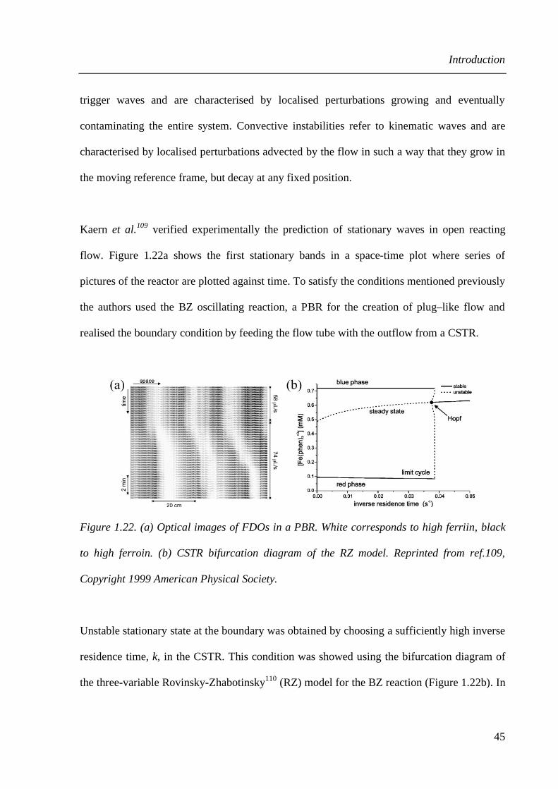
Introduction

45

trigger waves and are characterised by localised perturbations growing and eventually

contaminating the entire system. Convective instabilities refer to kinematic waves and are

characterised by localised perturbations advected by the flow in such a way that they grow in

the moving reference frame, but decay at any fixed position.

Kaern et al.109 verified experimentally the prediction of stationary waves in open reacting

flow. Figure 1.22a shows the first stationary bands in a space-time plot where series of

pictures of the reactor are plotted against time. To satisfy the conditions mentioned previously

the authors used the BZ oscillating reaction, a PBR for the creation of plug–like flow and

realised the boundary condition by feeding the flow tube with the outflow from a CSTR.

Figure 1.22. (a) Optical images of FDOs in a PBR. White corresponds to high ferriin, black

to high ferroin. (b) CSTR bifurcation diagram of the RZ model. Reprinted from ref.109,

Copyright 1999 American Physical Society.

Unstable stationary state at the boundary was obtained by choosing a sufficiently high inverse

residence time, k, in the CSTR. This condition was showed using the bifurcation diagram of

the three-variable Rovinsky-Zhabotinsky110 (RZ) model for the BZ reaction (Figure 1.22b). In

Introduction

46

the absence of a flow, the RZ model shows that the CSTR oscillates between the red and blue

phases. At a sufficiently high inverse residence time it switches from an oscillating state to a

stationary one. This stationary state CSTR output served as the inflow to the PBR.

In this thesis, space-time plots will be presented with time in the horizontal axis, as are the

results presented by Bamforth et al.111 (Figure 1.23).

Figure 1.23. Optical images of the FDO patterns in a PBR. Each image interval corresponds

to approximately 2 min. Reprinted from ref.111, Copyright 2002 PCCP owner societies.

1.5.3 Flow Distributed Oscillations (FDOs)

1.5.3.1 FDO mechanisms

Kaern et al.109 proposed a simplified model for the FDO formation where the contribution of

diffusion/dispersion is negligible and stationary waves are generated through a simple

kinematic mechanism where a batch oscillator (undergoing oscillations of period T) is

Introduction

47

spatially resolved in the presence of a constant flow of velocity U. If the phase of the

oscillation is fixed at the inlet, the oscillation phase will be locked in space and stationary

waves will emerge with a wavelength, λFDO, given by:

!

"FDO = U #T ( 1.23 )

Andresen et al.112 explained that this equation is an oversimplification of the phenomenon, as

it is not addressing neither the convective nature of the waves nor the criterion for amplifying

waves. In their approach, the perturbation at the inlet is compared to a particle moving at

velocity U and emitting waves at frequency ω = 1 / T, where T is the BZ reaction oscillation

period. The stationary case arises if the phase velocity of the waves is equal to the flow

velocity. To illustrate their point, they used a model110 describing the system used in the

Kaern et al.109 experiments. Their simulations showed that for a constant dispersion

coefficient the wavelength grows importantly with the flow velocity for low velocities but

relaxes to a linear dependence for high flow velocities. They suggested that a linear

relationship between the FDO wavelength and the flow velocity was perceived in the results

of Kaern et al.109 because the dispersion coefficient depended linearly on the flow velocity.

This reconciled the two models113: despite the fact that dispersion is not required for the

formation of stationary waves and plays only a secondary role (by altering λFDO), it has to be

sufficiently weak compared to the flow for the system to remain in the FDO domain. Above

the critical flow rate, the kinematic model applies when dispersion is negligible or

proportional to U. The dependency of λFDO on U will generally become non-linear in the

presence of important flow-induced dispersion.

Introduction

48

1.5.3.2 Wave generation mechanism and limit conditions

Following experimental studies of FDOs in PBRs revealed the limitations of the kinematic

model proposed by Kaern et al.109 The pattern formation mechanism observed by Taylor et

al.114 (Figure 1.24) involves a wave-splitting from successive oxidation pacemaker sites.

Once the wave appeares, part of it moves in the direction of the flow and disappears, while

the other propagates against the flow and settles as a stationary band. Equation 1.23 cannot

describe this behaviour. This mechanism was not observed in the work of Kaern et al.,

probably due to high flow rate.

Figure 1.24.Stationary pattern formation mechanism observed by Taylor et al.114 Reprinted

from ref.114, Copyright 2002 PCCP owner societies.

Wave-splitting is only observed at relatively low flow velocities, where dispersion can

compete with flow. Of course, depending on the chemical reaction used and the transport

properties of the system, the wave-splitting mechanism can be observed even at higher flow

rates.

Despite its ability to predict the linear relationship between the FDO wavelength and the flow

velocity observed in many experimental set-ups, the kinematic mechanism fails to analyse the

Introduction

49

FDO formation. The existence of a minimum flow rate for the observation of stationary

patterns was suggesting this limitation113. In their seminal paper on FDOs, Kaern and

Menzinger109 observed a linear dependence of λFDO on flow rate, but did not identify a critical

flow rate or observed any non-linear behaviour. The behaviour close to the critical flow rate

was to be studied. Bamforth et al.111 analysed theoretically the system dynamics for flow

velocities close to the transition from stationary patterns to travelling waves (Figure 1.25a).

Figure 1.25. (a)Theoretical space–time plots at low flow rate by Bamforth et al.111 and (b-c)

experimental space-time plots at low flow rate by Kaern et al.115 The flow velocity was of 0.03

cm s−1 for (b) and 0.001 cm s−1 for (c). (a) is reprinted from ref.111, Copyright 2002 PCCP

owner societies. (b) and (c) are reprinted from ref.115, Copyright 2002 American Chemical

Society.

In their model one or two bands could fail to stabilise after the wave-splitting before one

settles. This phenomenon was observed by Kaern et al.115 (Figure 1.25b). At even lower

flow, their results showed an FDO breakdown where the stationary patterns were replaced by

irregular travelling waves (Figure 1.25c).

Introduction

50

1.5.3.3 FDO wavelength and bands

Both Kaern et al.109 and Bamforth et al.111 noticed that λFDO was significantly shorter than the

wavelength predicted by the kinematic model (Equation 1.23), which they accounted for

enhanced dispersion. Hence, λFDO is shown to increase with flow rate and decrease with

dispersion.

The first study of the role of chemistry in the resulting patterns was made by Bamforth et

al.111, who added the concentrations of BrO3− and H+ to the kinematic model. The wavelength

of fully-developed patterns was predicted and experimentally verified to scale linearly with

the flow rate Q and the inverse square root of BrO3− and H+ concentrations:

!

"FDO ~ QBrO3

#[ ]1/ 2H+[ ]1/ 2 ( 1.24 )

A better understanding of the interplay between chemistry and flow in these systems was

provided by Britton et al.116 who used MRI to probe manganese-catalysed BZ FDOs in a

PBR, revealing the 3D shape of the Mn3+ bands. A radial concentration gradient was shown to

result in a V-shaped wave front (Figure 1.26). The authors related this shape to the

hydrodynamic properties of the reactor. The V-shape was explained by the radial variation of

the fluid velocity (faster by the walls of the PBR). These results showed that radial mixing is

playing an important role in this phenomenon by homogenising the medium and stressed the

limitations of 1D models in predicting the evolution of the experimental FDO system

behaviour.

Introduction

51

Figure 1.26. 3D renderings of a stationary FDO band in a PBR, at various orientations (a-d).

These images were produced using series of 2D MR images. The colour scale indicates the

position along the length of the reactor (blue is upstream and red is downstream). Shading

highlights the 3D structure of the wave. Reprinted from ref.116, Copyright 2005 American

Chemical Society.

1.5.3.4 Influencing parameters

Kaern and Menzinger identified the linear relationship between axial flow rate and

wavelength in their first FDO paper109. By changing the flow rate, they could observe that the

system was readapting its wavelength (Figure 1.22a). Bamforth et al.111 also studied the band

readjustment following a change in the flow rate. They observed a simple transition

mechanism to the new FDO wavelength. For a flow rate increase, FDO bands move upwards

initially keeping their original separation and amplitude. This movement increases the

distance separating the first band from the boundary layer that appears unaltered. The

amplitude of the first band also increases as it settles at its new stationary position. Following

this, the distance between this band and the second band increases. Similarly, the amplitude of

the second band increases as it reaches the appropriate separation from the first band and

Introduction

52

becomes stationary. This process repeats for all subsequent bands until the new stationary

pattern is fully established along the length of the reactor.

At flow velocities close to the critical velocity required for stationary patterns, a new type of

complex pattern was observed by Taylor et al.114. Stationary patterns were found to appear

after a transition period (Figure 1.27), the length of which depended sensitively on the flow

rate (with higher flow leading to quicker transition). A zigzag pattern observed when the

CSTR was close to the bifurcation point was found to depend sensitively on the initial

concentrations and flow velocity.

Figure 1.27. Complex pattern development close to the critical flow rate: Experimental

images of the BZ FDO in a PBR taken at 10 s intervals. (the vertical white line indicates a

break in time of 1 h). (a) Flow rate of 0.09 cm s−1, (b) 0.095 cm s−1. Reprinted from ref.114,

Copyright 2002 PCCP owner societies.

The authors discussed possible mechanisms, involving fluid phase fluctuations at the

boundary and packing material effects (PBR glass beads). They noticed that once established,

the stationary patterns were stable, such that if the flow was switched off and then on again,

Introduction

53

the patterns faded and then reappeared. However, if the flow was switched off prior to the

establishment of stationary patterns then phase waves propagated through the system from the

top of the tube to the bottom. For flow velocities less than a critical value (0.08 cm s−1 in their

experiments), the CSTR oscillated.

Other flow effects on FDO are related to diffusion and dispersion. At high flow rates,

dispersion was shown to play an important role in determining the wavelength of the

structure. Kaern et al.115 observed a significant λFDO decrease with increasing packing material

diffusion coefficient. At low flow velocity, where the stationary waves breakdown to irregular

wave structures, the critical flow velocity at which this breakdown occured was lowered when

the effective diffusion coefficient was decreased. These results confirm that a low ratio of

dispersive to advective transport coefficient is favourable to the formation of FDO waves.

Kaern et al.117 studied the influence of the boundary condition by probing travelling waves

that arose when the boundary oscillates. Far from the bifurcation point, waves propagate

along the reactor with an almost constant velocity. However, when the CSTR residence time

lies close to the bifurcation value, the waves propagate with an oscillatory velocity (Figure

1.28).

Introduction

54

Figure 1.28. Oscillatory wave propagation obtained by Kaern et al.117 White bands

correspond to high ferriin concentrations. The flow tube is fed by an oscillatory CSTR. The

residence time in the CSTR is lower than, but close to, the stationary bifurcation one.

Reprinted from ref.117, Copyright 2000 American Physical Society.

Novak et al.118 used a temperature sensitive agar gel system to study temperature effects on

FDOs. They investigated periodic temperature modulation forcing of FDOs in a tubular

reactor and observed synchronisation between the variation of band position and temperature

changes. Their results reflect the effect of temperature on both chemical oscillations in batch

reactors33,34 and agar gel.

Taylor et al.114 analysed the possible effect of the PBR glass beads on the FDO patterns. In

contact with aqueous solutions, glass beads posses a negative surface charge due to formation

of SiO− groups. Positively charged species in the BZ reaction, such as the metal catalyst

Fe(phen)32+/3+ and H2BrO2

+, may be affected by the negative surface groups. In this case, the

Introduction

55

system can switch from an equal dispersion system to a differential dispersion one. Such a

switch may exist when dispersion dominates over turbulent mixing, although this generally

occurs under lower flow rates (Re<0.1)119. The interactions of positive species with the beads

may help to explain the stability of the stationary pulses, once established, by ‘‘ locking’’ the

catalyst in oxidised mode. Also, Kaern et al.115 suggested that stagnant pockets of the fluid

could explain similar phenomena.

Finally, less dominant parameters as gravity36,120 or magnetic fields121 have been shown to

affect the propagation of BZ waves. Also, theoretical work22 suggests that convectively

unstable open flows as in FDO systems can behave as noise amplifiers and lead to the

formation of noise-sustained structures.

1.5.4 The general case of flow distributed structures and its applications

The combination of an RDA system with the effect of an initial boundary condition that leads

to FDOs can be considered as a specific case of a general category of stationary patterns.

Satnoianou et al.122 presented a theoretical study of coupled RDA system instabilities in one-

dimensional domains. These instabilities are creating spatially periodic stationary waves that

the authors termed flow and diffusion-distributed structures (FDS). FDOs and Turing patterns

are presented as particular cases of FDS instability. This work highlights that other FDS

should be easier to obtain in chemical systems showing how such structures might have a

crucial role in biological pattern formation.

Introduction

56

Indeed, FDO mechanisms have already been proposed as a means for explaining biological

pattern formation by Kaern et al.123 who applied the FDO kinematic model to the process of

somitogenesis. Somitogenesis refers to the formation of spatially repetitive structures along

the growth axis of a developing embryo. The authors argued that FDO conditions are satisfied

during chick and mouse somitogenesis. Similarly to FDO waves, gene expression waves

observed in these species arise from phase dynamics in a growing oscillatory medium.

Finally, aside the possible relevance of FDS to biological pattern formation, McGraw et al.124

identified FDS features shared with open flow systems in fluid mechanics and plasma physics

(convective instability, role of boundary conditions in the pattern selection).

(1) Tsuchiya, Y.; Yamazaki, H.; Aoki, T. Biophys. J. 1991, 59, 249.

(2) Neufeld, Z. Chaos 2012, 22.

(3) Nicolis, G.; Prigogine, I. Self-Organisation in Non-equilibrium Systems: From

Dissipative structures to Order through Fluctuations; John Wiley and Sons Inc., 1977.

(4) Haken, H. Synergetics; Springer-Verlag Berlin Heidelberg, 1978.

(5) Prigogine, I.; Stengers, I. Order out of Chaos: Man's new dialogue with

nature; Flamingo, 1984.

(6) Taylor, G. I. Philosophical Transactions of the Royal Society of London Series

a-Containing Papers of a Mathematical or Physical Character 1923, 223, 289.

(7) Tagg, R. A Guide to Literature Related to the Taylor-Couette Problem. In

Ordered and Turbulent Patterns in Taylor-Couette Flow; Andereck, C. D., Hayot, F., Eds.;

Springer US, 1992; pp 303.

(8) Wolinski, J.; Wronski, S. Chem. Eng. and Process. 2009, 48, 1061.

Introduction

57

(9) Resende, M. M.; Sousa, R.; Tardioli, P. W.; Giordano, R. L. C.; Giordano, R.

C. AIChE J. 2005, 51, 314.

(10) Ouyang, Q.; Castets, V.; Boissonade, J.; Roux, J. C.; Dekepper, P.; Swinney,

H. L. J. Chem. Phys. 1991, 95, 351.

(11) Deng, R. S.; Arifin, D. Y.; Mak, Y. C.; Wang, C. H. AIChE J. 2009, 55, 3056.

(12) Dusting, J.; Balabani, S. Chem. Eng. Sci. 2009, 64, 3103.

(13) Britton, M. M. Chem. Soc. Rev. 2010, 39, 4036.

(14) Haken, H. Information and self-organization : a macroscopic approach to

complex systems, 3rd enl. ed.; Springer: Berlin ; New York, 2006.

(15) Vallatos, A.; Wilson, M. C. T.; Taylor, A. F.; Britton, M. M. Europhys. Lett.

2012, 99.

(16) Vallatos, A.; Evans, R. D.; Taylor, A. F.; Britton, M. M. Chaos 2013, 23.

(17) Scott, S.-K. Oscillations, Waves, and chaos in Chemical Kinetics Oxford

University Press, 1994.

(18) Scott, S. K.; Showalter, K. J. Phys. Chem. 1992, 96, 8702.

(19) Zhabotinsky, A. M. Biofizika 1964, 9.

(20) Noyes, R. M.; Field, R. J.; Koros, E. J. Am. Chem. Soc. 1972, 94, 1394.

(21) Field, R. J.; Noyes, R. M.; Koros, E. J. Am. Chem. Soc. 1972, 94, 8649.

(22) Kuznetsov, S. P.; Mosekilde, E.; Dewel, G.; Borckmans, P. J. Chem. Phys.

1997, 106, 7609.

(23) Thompson, B. W.; Novak, J.; Wilson, M. C. T.; Britton, M. M.; Taylor, A. F.

Phys. Rev. E 2010, 81.

(24) Field, R. J.; Burger, M. Oscillations and traveling waves in chemical systems;

Wiley: New York, 1985.

Introduction

58

(25) Burger, M.; Koros, E. J. Phys. Chem. 1980, 84, 496.

(26) Körös, E.; Murger, M.; Friedrich, V.; Ladányi, L.; Nagy, Z.; Orbán, M.

Faraday Symp. Chem. S. 1974, 9.

(27) Zhabotinsky, A. M. Chaos 1991, 1, 8.

(28) Gao, Y.; Cross, A. R.; Armstrong, R. L. J. Phys. Chem. 1996, 100, 10159.

(29) Schlüter, A.; Weiss, A. Berichte der Bunsengesellschaft für physikalische

Chemie 1981, 85, 306

(30) Hansen, E. W.; Ruoff, P. J. Phys. Chem. 1989, 93, 264.

(31) Koros, E.; Orban, M. Nature 1978, 273, 371.

(32) Greenwood, N. N.; Earnshaw, A. Chemistry of the elements, 2nd ed.;

Butterworth-Heinemann: Oxford ; Boston, 1997.

(33) Dutt, A. K.; Menzinger, M. J. Phys. Chem. 1992, 96, 8447.

(34) Dutt, A. K.; Muller, S. C. J. Phys. Chem. 1993, 97, 10059.

(35) Treindl, L.; Ruoff, P.; Kvernberg, P. O. J. Phys. Chem. A 1997, 101, 4606.

(36) Fujieda, S.; Mori, Y.; Nakazawa, A.; Mogami, Y. Adv. Space Res. 2001, 28, 8.

(37) Zaikin, A. N.; Zhabotin.Am. Nature 1970, 225, 535.

(38) Epstein, I. R. P. Natl. Acad. Sci. USA 2006, 103, 15727.

(39) Noszticzius, Z.; Horsthemke, W.; Mccormick, W. D.; Swinney, H. L.; Tam,

W. Y. Nature 1987, 329, 619.

(40) Steinbock, O.; Siegert, F.; Muller, S. C.; Weijer, C. J. P. Natl. Acad. Sci. USA

1993, 90, 7332.

(41) Zhou, C. S.; Kurths, J. New Journal of Physics 2005, 7.

(42) Shlesinger, M. F.; Zaslavsky, G. M.; Klafter, J. Nature 1993, 363, 31.

(43) Young, W.; Pumir, A.; Pomeau, Y. Phys. Fluids a-Fluid 1989, 1, 462.

Introduction

59

(44) Meiss, J. D.; Ott, E. Phys. Rev. Lett. 1985, 55, 2741.

(45) Zumofen, G.; Klafter, J.; Shlesinger, M. F. Anomalous Diffusion: From Basics

to Applications 1999, 519, 15.

(46) Solomon, T. H.; Weeks, E. R.; Swinney, H. L. Phys. Rev. Lett. 1993, 71, 3975.

(47) Solomon, T. H.; Tomas, S.; Warner, J. L. Phys. Rev. Lett. 1996, 77, 2682.

(48) Paoletti, M. S.; Solomon, T. H. Phys. Rev. E 2005, 72.

(49) Solomon, T. H.; Mezic, I. Nature 2003, 425, 376.

(50) Frankel, I.; Brenner, H. J. Fluid Mech. 1989, 204, 97.

(51) Metcalfe, I. S. Chemical reaction engineering : a first course; Oxford

University Press: Oxford ; New York, 1997.

(52) Levenspiel, O. Chemical reaction engineering, 3rd ed.; Wiley: New York,

1999.

(53) Koschmieder, E.-L. Benard Cells and Taylor Vortices; Cambridge University

Press, 1993.

(54) Meyer-Spasche, R. Pattern Formation in Viscous Flows – The Taylor Couette

Problem and Rayleigh-Benard Convection; Birkhauser 1999.

(55) Giordano, R. C.; Giordano, R. L. C.; Prazeres, D. M. F.; Cooney, C. L. Chem.

Eng. Sci. 1998, 53, 3635.

(56) Desmet, G.; Verelst, H.; Baron, G. V. Chem. Eng. Sci. 1996, 51, 1287.

(57) Desmet, G.; Verelst, H.; Baron, G. V. Chem. Eng. Sci. 1996, 51, 1299.

(58) Ohmura, N.; Okamoto, H.; Makino, T.; Kataoka, K. J. Chem. Eng. Jpn 2002,

35, 692.

(59) Richter, O.; Menges, M.; Kraushaar-Czarnetzki, B. Chem. Eng. Sci. 2009, 64,

2384.

Introduction

60

(60) Kose, K. Phys. Rev. Lett. 1994, 72, 1467.

(61) Hopkins, J. A.; Santini, R. E.; Grutzner, J. B. J. Magn. Res. Ser. A 1995, 117,

150.

(62) Seymour, J. D.; Manz, B.; Callaghan, P. T. Phys. Fluids 1999, 11, 1104.

(63) Gu, Z. H.; Fahidy, T. Z. Can. J. Chem. Eng. 1985, 63, 710.

(64) Lueptow, R. M.; Docter, A.; Min, K. Y. Phys. Fluids a-Fluid 1992, 4, 2446.

(65) Giordano, R. L. C.; Giordano, R. C.; Prazeres, D. M. F.; Cooney, C. L. Chem.

Eng. Sci. 2000, 55, 3611.

(66) Buchel, P.; Lucke, M.; Roth, D.; Schmitz, R. Phys. Rev. E 1996, 53, 4764.

(67) Wereley, S. T.; Lueptow, R. M. Phys. Fluids 1999, 11, 3637.

(68) Moser, K. W.; Raguin, L. G.; Harris, A.; Morris, H. D.; Georgiadis, J.;

Shannon, M.; Philpott, M. Magn. Reson. Imaging 2000, 18, 199.

(69) Coles, D. J. Fluid Mech. 1965, 21.

(70) Chandrasekhar, S. Hydrodynamic and Hydromagnetic Stability, 1961.

(71) Recktenwald, A.; Lucke, M.; Muller, H. W. Phys. Rev. E 1993, 48, 4444.

(72) Howes, T.; Rudman, M. AIChE J. 1998, 44, 255.

(73) Kataoka, K.; Hongo, T.; Futagawa, M. J. Chem. Eng. Jpn 1974, 8, 4.

(74) Legrand, J.; Coeuret, F. Chem. Eng. Sci. 1986, 41, 47.

(75) Haim, D.; Pismen, L. M. Chem. Eng. Sci. 1994, 49, 1119.

(76) Judat, B.; Racina, A.; Kind, M. Chem. Eng. Technol. 2004, 27, 287.

(77) Forney, L. J.; Pierson, J. A. AIChE J. 2003, 49, 727.

(78) Haut, B.; Ben Amor, H.; Coulon, L.; Jacquet, A.; Halloin, V. Chem. Eng. Sci.

2003, 58, 777.

Introduction

61

(79) Sczechowski, J. G.; Koval, C. A.; Noble, R. D. Chem. Eng. Sci. 1995, 50,

3163.

(80) Campero, R. J.; Vigil, R. D. Chem. Eng. Sci. 1997, 52, 3303.

(81) Syed, A.; Fruh, W. G. J. Chem. Technol. Biot. 2003, 78, 227.

(82) Raguin, L. G.; Georgiadis, J. G. J. Fluid Mech. 2004, 516, 125.

(83) Gladden, L. F.; Sederman, A. J. Journal of Magnetic Resonance 2013, 229, 2.

(84) Ross, J.; Muller, S. C.; Vidal, C. Science 1988, 240, 460.

(85) Ortoleva, P.; Ross, J. J. Chem. Phys. 1974, 60, 5090.

(86) Winfree, A. T. Science 1973, 181, 937.

(87) Pojman, J. A.; Epstein, I. R.; Mcmanus, T. J.; Showalter, K. J. Phys. Chem.

1991, 95, 1299.

(88) Menzinger, M.; Tzalmona, A.; Armstrong, R. L.; Cross, A.; Lemaire, C. J.

Phys. Chem. 1992, 96, 4725.

(89) Wu, Y. Q.; Vasquez, D. A.; Edwards, B. F.; Wilder, J. W. Phys. Rev. E 1995,

51, 1119.

(90) Nugent, C. R.; Quarles, W. M.; Solomon, T. H. Phys. Rev. Lett. 2004, 93.

(91) Paoletti, M. S.; Nugent, C. R.; Solomon, T. H. Phys. Rev. Lett. 2006, 96.

(92) Paoletti, M. S.; Solomon, T. H. Europhys. Lett. 2005, 69, 819.

(93) Mahoney, J.; Bargteil, D.; Kingsbury, M.; Mitchell, K.; Solomon, T. Europhys.

Lett. 2012, 98.

(94) Lauffer, R. B. Chem. Rev. 1987, 87, 901.

(95) Tzalmona, A.; Armstrong, R. L.; Menzinger, M.; Cross, A.; Lemaire, C. Chem.

Phys. Lett. 1990, 174, 199.

Introduction

62

(96) Tzalmona, A.; Armstrong, R. L.; Menzinger, M.; Cross, A.; Lemaire, C. Chem.

Phys. Lett. 1992, 188, 457.

(97) Cross, A. R.; Armstrong, R. L.; Reid, A.; Su, S. Y.; Menzinger, M. J. Phys.

Chem. 1995, 99, 16616.

(98) Cross, A. L.; Armstrong, R. L.; Gobrecht, C.; Paton, M.; Ware, C. Magn.

Reson. Imaging 1997, 15, 719.

(99) Koptyug, I. V.; Lysova, A. A.; Parmon, V. N.; Sagdeev, R. Z. Kinet. Catal.

2003, 44, 401.

(100) Koptyug, I. V.; Lysova, A. A.; Matveev, A. V.; Ilyina, L. Y.; Sagdeev, R. Z.;

Parmon, V. N. Magn. Reson. Imaging 2003, 21, 337.

(101) Hennig, J.; Nauerth, A.; Friedburg, H. Magn. Reson. Med. 1986, 3, 823.

(102) Britton, M. M. J. Phys. Chem. A 2006, 110, 2579.

(103) Taylor, A. F.; Britton, M. M. Chaos 2006, 16.

(104) Marek, M.; Svobodova, E. Biophys. Chem. 1975, 3, 263.

(105) Turing, A. M. Philos. T. Roy. Soc. B. 1952, 237, 37.

(106) Castets, V.; Dulos, E.; Boissonade, J.; Dekepper, P. Phys. Rev. Lett. 1990, 64,

2953.

(107) Rovinsky, A. B.; Menzinger, M. Phys. Rev. Lett. 1993, 70, 778.

(108) Andresen, P.; Bache, M.; Mosekilde, E.; Dewel, G.; Borckmans, P. Phys. Rev.

E 1999, 60, 297.

(109) Kaern, M.; Menzinger, M. Phys. Rev. E 1999, 60, R3471.

(110) Zhabotinsky, A. M.; Rovinsky, A. B. J. Phys. Chem. 1990, 94, 8001.

(111) Bamforth, J. R.; Toth, R.; Gaspar, V.; Scott, S. K. Phys. Chem. Chem. Phys.

2002, 4, 1299.

Introduction

63

(112) Andresen, P.; Mosekilde, E.; Dewel, G.; Borckmans, P. Phys. Rev. E 2000, 62,

2992.

(113) Kaern, M.; Menzinger, M. Phys. Rev. E 2000, 62, 2994.

(114) Taylor, A. F.; Bamforth, J. R.; Bardsley, P. Phys. Chem. Chem. Phys. 2002, 4,

5640.

(115) Kaern, M.; Menzinger, M. J. Phys. Chem. A 2002, 106, 4897.

(116) Britton, M. M.; Sederman, A. J.; Taylor, A. F.; Scott, S. K.; Gladden, L. F. J.

Phys. Chem. A 2005, 109, 8306.

(117) Kaern, M.; Menzinger, M. Phys. Rev. E 2000, 61, 3334.

(118) Novak, J.; Thompson, B. W.; Wilson, M. C. T.; Taylor, A. F.; Britton, M. M.

Phys. Chem. Chem. Phys. 2011, 13, 12321.

(119) Yu, D.; Jackson, K.; Harmon, T. C. Chem. Eng. Sci. 1999, 54, 357.

(120) Fujieda, S.; Mogami, Y.; Zhang, W.; Shinohara, H.; Handa, S. Anal. Sci. 1999,

15, 159.

(121) Okano, H.; Kitahata, H.; Akai, D. J. Phys. Chem. A 2009, 113, 3061.

(122) Satnoianu, R. A.; Maini, P. K.; Menzinger, M. Physica D 2001, 160, 79.

(123) Kaern, M.; Menzinger, M.; Hunding, A. J. Theor. Biol. 2000, 207, 473.

(124) Mcgraw, P. N.; Menzinger, M. Phys. Rev. E 2003, 68.

Magnetic resonance techniques

64

2 Magnetic resonance techniques

2.1 Magnetic resonance principles

Only an overview to the theory behind NMR and MRI will be given in this section. For

further information, one may refer to the numerous textbooks on the subject1−4.

Magnetic resonance (MR) probes the behaviour of nuclei that possess nuclear spin. A

spinning nucleus possesses angular momentum, P, and charge and it is the motion of this

charge that gives rise to an associated magnetic moment, µ (Figure 2.1a). The magnetic

moment and angular momentum of a nucleus are vector quantities related to each other by

the magnetogyric ratio, γ, which gives a measure of how ‘strongly magnetic’ the nucleus is:

!

µ = "P ( 2.1 )

Although several nuclei possess spin property, this thesis will consider only hydrogen, 1H,

since it is both the most imaged nucleus in MRI and the only one probed in this work. In the

presence of a static magnetic field, the magnetic moment of the 1H nuclei will orient relative

to the field. The number of possible orientations, or energy states5, is determined by the spin

quantum number, I. 1H has spin number of 1/2 and can adopt two possible orientations with

respect to the field (Figure 2.1b): a low energy one (m = –1/2), where the nuclear spin vector

is in the same direction as the field (spin-up), and a high energy one (m = +1/2), where the

nuclear spin vector is in the opposite direction (spin-down).

Magnetic resonance techniques

65

In addition to this alignment, 1H nuclei will precess at a frequency ω, called the Larmor

frequency, that will depend on γ, and the field strength, B0.

!

" = #$B0 ( 2.2 )

Figure 2.1 (a) The magnetic field causes the nucleus to precess at the Larmor frequency. (b)

Schematic diagram showing the degenerate states of 1H.

At thermal equilibrium, there is a Boltzmann distribution of nuclei between the two energy

levels with an excess of the lower energy spin-up nuclei. An ensemble average of all the spin

magnetic moments produces a macroscopic magnetisation6, M0 , along the direction of B0

(Figure 2.2).

Figure 2.2. Formation of the magnetisation vector, M0, at thermal equilibrium.

Magnetic resonance techniques

66

Typically, the field is applied in the z direction, Bz, and the net magnetisation becomes Mz.

NMR experiments manipulate M using radiofrequency (rf) pulses to induce transitions

between spin states leading to a deflection of the magnetisation. The degree to which the

magnetisation is deflected (tip angle, θ) is dependent on the amplitude and duration of the rf

pulse. A 90˚ rf pulse in the y-direction (90˚y) will rotate the bulk magnetisation vector from

the z axis to the x axis as shown in Figure 2.3a. The magnetisation precesses at the Larmor

frequency in the xy-plane and can induce a current in coils. The measured signal is called the

free induction decay (FID) and will reduce over time due to spin relaxation processes.

Figure 2.3. (a) Schematic diagram showing a 90˚y pulse rotating the net magnetisation

vector, M, from the z-axis to the x-axis. (b) NMR signal measured by coils as M precesses on

the xy-plane.

Magnetic field variations caused by different chemical environments on spins will cause

variations in the Larmor frequency. These deviations are called chemical shifts and are the

basis of NMR spectroscopy. By using a reference frame rotating at the Larmor frequency, it is

possible to resolve frequency deviations related to chemical shift and get an insight regarding

the chemistry of the system. The different frequencies at which the FID oscillates can be used

to characterise various chemical environments experienced by the spins. Fourier

transformation of the FID produces a spectrum, revealing frequency offsets with respect to a

Magnetic resonance techniques

67

reference. This is the NMR spectrum and probably is one of the most used tools for chemical

characterisation. But the relaxation time taken by the spins to regain their equilibrium position

after the rf pulse is also characteristic of their chemical environment and can therefore be used

for chemical characterisation.

2.2 Magnetic resonance relaxation

MR relaxation is defined by two relaxation times related to two processes that characterise the

rate of return to equilibrium after an rf pulse is applied:

• T1 relaxation time determines the rate at which the ratio of spin-up to spin-down

nuclei returns to thermal equilibrium.

• T2 relaxation time determines the rate at which nuclear spins loose the phase

coherence gained by the application of the rf pulse.

2.2.1 T1 relaxation

T1 relaxation refers to the return of the magnetisation to the equilibrium value, Mz. The

relaxation rate depends on local fluctuations in the magnetic field. T1 relaxation is an

exponential decay process described by:

!

M z = M0(1" 2e("t /T1 ) ) ( 2.3 )

Measurement of T1 relaxation is typically achieved using an inversion recovery experiment7,

the pulse sequence for which is shown in Figure 2.4. In this experiment, the macroscopic

magnetisation is inverted by a 180˚ pulse, so that it resides along the negative z-axis. The

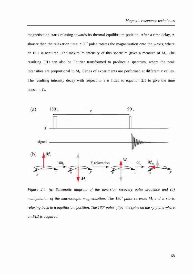
Magnetic resonance techniques

68

magnetisation starts relaxing towards its thermal equilibrium position. After a time delay, τ,

shorter than the relaxation time, a 90˚ pulse rotates the magnetisation onto the y-axis, where

an FID is acquired. The maximum intensity of this spectrum gives a measure of Mz. The

resulting FID can also be Fourier transformed to produce a spectrum, where the peak

intensities are proportional to Mz. Series of experiments are performed at different τ values.

The resulting intensity decay with respect to τ is fitted to equation 2.1 to give the time

constant T1.

Figure 2.4. (a) Schematic diagram of the inversion recovery pulse sequence and (b)

manipulation of the macroscopic magnetisation: The 180˚ pulse reverses Mz and it starts

relaxing back to it equilibrium position. The 180˚ pulse ‘flips’ the spins on the xy-plane where

an FID is acquired.

Magnetic resonance techniques

69

2.2.2 T2 relaxation

T2 relaxation refers to the relaxation of spins in the transverse plane. This occurs when,

following an rf pulse, local magnetic field strength variations cause spins to loose phase

coherence in the xy-plane, because of the existence of different precession frequencies. This

loss of phase coherence is described by an exponential relationship:

!

Mx,y = M0e("t /T2 ) ( 2.4 )

The Hahn echo, or spin echo, experiment is used for the measurement of transverse

relaxation8. The pulse sequence producing a Hahn echo and the behaviour of the

magnetisation are shown in Figure 2.5.

Figure 2.5. Schematic diagram showing (a) a Hahn echo pulse sequence and (b)

manipulation of spins: The 90˚ pulse rotates M into the xy-plane and the spins begin to loose

phase coherence. The 180˚ pulse ‘flips’ the spins, which start refocusing until an echo is

formed.

Magnetic resonance techniques

70

A 90˚ rf pulse rotates the magnetisation into the xy-plane, following which spins begin to

loose phase coherence, with some precessing faster and some slower. After a period τ, the

spins are inverted by a 180˚ rf pulse causing them to rotate in the opposite direction until they

regain the previously lost phase coherence. An echo occurs when the spins are completely

refocussed, after a time τ following the application of the 180˚ rf. The Hahn echo experiment

is, however, very sensitive to magnetic field inhomogeneities and diffusion. If spins diffuse to

a region with a slightly different magnetic field, they cannot be fully refocused by the 180˚

pulse. As a result, in the presence of significant local field inhomogeneities (ΔB0), the

relaxation time of the FID is significantly shorter than T2. This relaxation time is called T2*.

The relation between T2 and T2* is given by:

!

1T2

* =1

T2("B0 )

+1T2

( 2.5 )

For measuring T2, and not T2*, the spins need to be refocused on a timescale where the

effects of diffusion are minimal. This is achieved using the Carr-Purcell-Meiboom-Gill

(CPMG) experiment8,9 (Figure 2.6), which repeats the 180˚ pulse n times, acquiring an echo

each time and then fitting the decay of the echoes to equation 2.4 to obtain T2.

Magnetic resonance techniques

71

Figure 2.6. (a) Schematic diagram showing the CPMG pulse sequence. The 180˚ pulse is

repeated n times with n echoes acquired. (b) Acquired echo train.

T1 and T2 relaxation times are characteristic of the chemical and physical environment of the

protons in a system and are used to produce contrast in MR images.

2.3 Magnetic Resonance Imaging (MRI)

2.3.1 Using magnetic gradients for spatial encoding

By applying magnetic field gradients, it is possible to obtain spatial information about a

sample. The static magnetic field varies linearly in the direction of the applied gradient

causing the precessional frequency of nuclei to become spatially dependent:

!

"(r ) = #B0 + #G • r ( 2.6 )

where G is the magnetic gradient and r is the position.

Magnetic resonance techniques

72

Application of a magnetic field gradient generates a helix of phase of the precessing nuclear

spin packets (Figure 2.7). To characterise the behavior of the phase of spin packets under the

influence of the gradient, one can use the wavelength of this helix, λ, over which a 360° phase

shift occurs. λ is dependent on the duration of the gradient, t, and the gradient strength G.

!

" =2#$Gt

( 2.7 )

Figure 2.7. (a) Spin packet phase following a 90° pulse without applied magnetic field

gradient. (b) Spin packet phase following a 90° pulse with a linear magnetic field gradient

applied (here in the z-direction) winding a helix of phase of wavelength λ.

Magnetic resonance techniques

73

2.3.2 k-space

In 1973, Mansfield10 introduced the concept of reciprocal space vector k, defined as:

!

k ="Gt2#

= $%1 ( 2.8 )

The k-space approach introduces a unit that is linearly varying on the experimental

parameters G and t in the direction of the gradient. That means that the k-space axes can be

traversed either by varying the gradient strength either by varying the duration of the gradient

application. This provides with two methods to encode the spatial information in MRI: phase

encoding (varying G at constant time) and frequency (or read) encoding (varying t at constant

G). In frequency encoding the gradient is switched on during the acquisition. A Fourier

transformation of this data produces a spatially dependent intensity plot. The resulting signal

intensity is proportional to the number of spins at a particular frequency. For a one-

dimensional frequency encoded experiment where a single frequency-encoding gradient is

applied along the z-axis, the resultant spectrum is a one-dimensional profile of all the spins in

the x and y axes projected onto the z-axis. Figure 2.8 shows an example of a 1D frequency

encoding of two tubes of water.

Figure 2.8. Frequency encoding spin density profile of two water tubes obtained when a

gradient is applied along z.

Magnetic resonance techniques

74

For phase encoding, a gradient pulse is used, which is switched on then off, before the signal

acquisition. The magnetic field gradient winds a helix of phase of the spin packets along an

axis (Figure 2.7b). When the gradient is switched off the spin packets maintain their position-

dependent phase.

By combining frequency and phase encoding along different axes it is possible to produce

two-dimensional images. Figure 2.9 shows a k-space raster with a frequency-encoded x-

direction and a phase encoded y-direction. A k-space raster is a representation of the data

points acquired for a 2D image and has the same number of points as the number of pixels in

the image.

Figure 2.9. Sampling of a k-space raster. The x and y direction gradients are responsible for

the frequency(read) and phase encoding respectively.

By applying gradients along the x and y directions it is possible to traverse this raster in Δk

steps. Δkx is the x-direction sampling interval given by

!

"kx = #Gx"tx / 2$ , where Δtx is the

sampling interval of the FID. By applying a negative gradient prior to the positive read

Magnetic resonance techniques

75

gradient it is also possible to traverse negative values of kx. Δky is the y-direction sampling

interval given by

!

"k y = #"Gyt y/2p , where ΔGy is the phase encoding step size. ky is traversed

through the application of successive phase encoding gradient steps.

By applying frequency and phase encoding gradients it is possible to produce a 2D data set in

k-space. A Fourier transformation of k-space data in both directions results in a space-domain

spectrum where the signal intensity is proportional to the number of spins at a particular

location on the xy-plane. The resultant real-space data is a 2D profile of all the spins in the

third dimension projected onto the encoding plane. To obtain a 2D image, a selection of spins

in a plane through the sample of interest, or slice selection, must be performed.

2.3.3 Slice selection

Slice selection11 along horizontal or vertical planes is achieved by simultaneously applying a

magnetic field gradient and a frequency selective rf pulse (Figure 2.10).

Figure 2.10. Horizontal (a) and vertical (b) slice selection through a cylindrical sample. The

grey region is the observable region of the rf coil, or field-of-view.

Magnetic resonance techniques

76

The magnetic field gradient causes nuclei to precess with different frequencies along the

desired direction for the slice selection. Using a soft, frequency-selective, rf pulse (Gaussian

or sinc function), it is possible to control the bandwidth of excited frequencies (inversely

proportional to the rf pulse duration).

The slice gradient causes an undesirable spread of the magnetisation vectors from different

regions of the sample, leading to reduced signal. To cancel out the spread in magnetization, a

refocusing gradient needs to be applied after the slice selection. This can be done either with

gradient of opposite sign following the slice gradient, either by a gradient of same sign

following a 180o rf pulse (Figure 2.10).

2.3.4 Spin echo imaging

Different imaging sequences can be produced by combining frequency encoding, phase

encoding and slice selection sequences. A spin echo imaging sequence is based on the use of

90o and 180o rf pulses to form a Hahn echo (Figure 2.11). Initially, a slice-selective pulse is

applied. The refocusing gradient produces a gradient echo. One single phase encoding

gradient is then applied on the excited spins. In order to refocus the magnetisation, a 180o rf

pulse is used to produce a Hahn echo. Following the application of the rf pulse, the spins are

frequency-encoded for position. The echo is formed in the middle of the frequency-encoding

gradient. The time between the centre of the 90o rf pulse and the centre of the echo is called

echo time TE. The data is acquired during the frequency encoding allowing for a full k-space

line to be acquired. The process is repeated for all increasing phase encoding gradients until

all k-space lines are acquired. TR is the repetition time.

Magnetic resonance techniques

77

Figure 2.11. Schematic representation of a spin echo imaging sequence.

The imaging experiment time is depending on the number of phase encoding pixels, nPE, the

repetition time between experiments, TR, and the number of image repetitions, nREP. It can be

calculated by:

!

Experiment time = nPE "TR " nREP ( 2.9 )

Two-dimensional Fourrier transformation of the data along the frequency and phase encoding

directions allows producing a real space image. Multiple slices can be excited sequentially

through different spatial locations of the sample and put together for the generation of 3D

images of the sample.

Magnetic resonance techniques

78

2.3.5 MRI contrast

There are four main ways through which contrast can be achieved in MR imaging: spin

density, relaxation times, chemical shift and spin motion. By varying the operating conditions

of the pulse sequence it is possible to favour one or another type of contrast.

Equation 2.10 gives a typical expression of the signal intensity at a position r arising from an

imaging experiment. In this expression, aH is the amplitude of the Hahn-echo.

!

aH(r,TR ,TE ) = M0(r ) 1" exp "TR

T1(r )#

$ %

&

' (

)

* +

,

- . exp "

TE

T2(r )#

$ %

&

' ( ( 2.10 )

Spin density contrast is obtained by variations of the number of excited spins within a sample.

The resulting images are called spin density maps. To eliminate relaxation time contrast and

obtain a spin density map, the effects of the exponential terms in Equation 2.10 must be

minimised. This can be achieved if the echo time, TE, is much shorter than T2 and the

repetition time, TR, is significantly longer than T1.

Relaxation contrast is obtained when the pulse sequence characteristic times are comparable

to the relaxation ones. To obtain T2 contrast, TE must be comparable to T2, in order to achieve

significant signal attenuation from the factor exp(–TE / T2). As for spin density contrast, to

ensure that T1 contrast is minimised, TR needs to be significantly longer than T1. Contrast on a

T2–weighted image corresponds to relaxation time differences between regions of the sample,

with bright regions typically corresponding to high T2 relaxation regions. Similarly, to obtain

T1 contrast, TR must be comparable to T1 in order to achieve significant signal attenuation

from the factor exp(–TR / T1). As for spin density contrast, to minimise T2 contrast on a T1-

Magnetic resonance techniques

79

weighted image the echo time must be as close as possible to zero (significantly smaller than

T2). Contrast on a T1–weighted image corresponds to relaxation time differences between

regions of the sample, but contrary to T2–weighted images, short relaxation times give high

signal intensity. Due to this difference, when an image contrast is obtained through a

combination of T1- and T2-weighted contrast, a parameter region where the two types of

contrast cancel out can be observed.

Chemical shift contrast is based on selective excitement of regions that have a particular

chemical shift. Exciting a narrow spectral region is obtained in a similar way to the slice

selection presented previously. Chemical shift contrast images are formed with signal coming

only from the selected regions.

Finally, motional contrast is obtained by combining an imaging sequence with a pulse

gradient spin echo sequence (PGSE) that allows encoding for motion. This method that

provides with velocity and diffusion/dispersion information within a sample is of particular

interest to this work.

2.4 Measurement of molecular motion

2.4.1 Pulsed gradient spin echo principles

In order to measure transport processes such as velocity or diffusion, a technique based on the

use of spin echoes is applied. The formation of an echo is based on the cancellation of

precessional phase shifts by reversing the phase evolution using a magnetic field gradient.

Magnetic resonance techniques

80

Over the time scale of the echo, molecular movements will produce additional phase shifts

that will not be refocused. The phase shifts in the resulting signal can be used to quantify

molecular movements.

The measure of translational motion can be obtained using a pulsed gradient spin echo

(PGSE) experiment6,12 (Figure 2.12).

Figure 2.12. PGSE experiment. During Δ, a spin packet migrates by Z, resulting in a phase

shift ϕ = γδgZ.

Magnetic resonance techniques

81

A 90o rf pulse bringing the net magnetisation in the transverse plane is followed by a short

duration gradient that winds a helix of phase of the spin packet magnetisation vectors. A 180o

rf pulse flips the vectors before a second gradient unwinds the helix of phase, refocusing all

the vectors. Any motion of the molecules during the time Δ between the two gradients will

result in a phase shift ϕ depending on the experiment parameters and the displacement of the

molecules. As for the imaging experiments, a reciprocal q-space representing spatial

frequency can be introduced. Similarly to the concept of reciprocal k-space, q-space has an

inverse relation to the spatial wavelength of the helix phase, allowing to link distances to the

gradient strength:

!

q ="#g2$

( 2.11 )

Stejskal13 showed that if the approximation of narrow δ pulses is valid (δ << Δ), so that we

can neglect motion occurring during their duration, it becomes possible to characterise

molecular displacements using the propagator formalism introduced in Chapter 1. To do this,

one has to define ρ(r) as the molecular density and ρ(r)P(r’r, Δ) as the probability for an

individual spin to start from r and finish at r’ during Δ. For each molecule, the phase shift

after the second gradient pulse would be equal to

!

"# = $g% & ( ' r ( r ) = q & ( ' r ( r ) and its

contribution to the echo signal E(q,Δ) - defined as the amplitude of the echo at its centre -

would be given by the term

!

exp(i"g# $ [ % r & r]) . Considering an ensemble of molecules one

can then write:

!

E(q,") = #(r )$ P(r % r ,")exp(iq & [ % r ' r])d % r dr$ ( 2.12 )

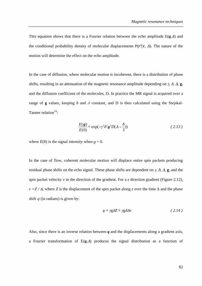
Magnetic resonance techniques

82

This equation shows that there is a Fourier relation between the echo amplitude E(q,Δ) and

the conditional probability density of molecular displacements P(r’r, Δ). The nature of the

motion will determine the effect on the echo amplitude.

In the case of diffusion, where molecular motion is incoherent, there is a distribution of phase

shifts, resulting in an attenuation of the magnetic resonance amplitude depending on γ, δ, Δ, g,

and the diffusion coefficient of the molecules, D. In practice the MR signal is acquired over a

range of g values, keeping δ and Δ constant, and D is then calculated using the Stejskal-

Tanner relation14:

!

E(g)E(0)

= exp("# 2$2g2D(% " $3

)) ( 2.13 )

where E(0) is the signal intensity when g = 0.

In the case of flow, coherent molecular motion will displace entire spin packets producing

residual phase shifts on the echo signal. These phase shifts are dependent on γ, δ, Δ, g, and the

spin packet velocity v in the direction of the gradient. For a z direction gradient (Figure 2.12),

v =Z / Δ, where Z is the displacement of the spin packet along z over the time Δ and the phase

shift ϕ (in radians) is given by:

!

" = #g$Z = #g$%v ( 2.14 )

Also, since there is an inverse relation between q and the displacements along a gradient axis,

a Fourier transformation of E(q,Δ) produces the signal distribution as a function of

Magnetic resonance techniques

83

displacements. By normalising this signal one obtains a propagator giving the probability of

molecular displacements along this axis (Figure 2.13).

Figure 2.13. A Fourier transformation of E(q), followed by a normalisation, gives a

propagator P(Z,Δ) representing the average probability of molecular displacements along z.

The propagator showed corresponds to molecules diffusing (D) and flowing at constant

average velocity (vz) along the gradient axis z.

To obtain an accurate measurement of the propagator it is necessary to increase the gradient

strength until the echo attenuation is less than 1%. As discussed in 1.4.1, the broadening of

the propagator depends on both diffusion and dispersion, while its shifting along the axis

depends on velocity (coherent flow). This allows deducing diffusion/dispersion by computing

the width of the propagator and mean velocity by computing the offset of the propagator.

When velocity gradients in the system are sufficiently high, as Δ increases, the effects of

diffusion on the molecular displacements become negligible and the broadening of the

propagator is dominated by flow-induced dispersion.

Magnetic resonance techniques

84

2.4.2 PGSE and PGSTE

Two pulsed gradient pulse sequences will be used in this thesis, the pulsed gradient spin echo

(PGSE) and the pulsed gradient stimulated echo (PGSTE) (Figure 2.14).

Figure 2.14. PGSE (a) and PGSTE (b) pulse sequences.

In terms of motion encoding, both sequences are equivalent, their difference lying only in the

way the signal relaxes. With the PGSE sequence the magnetisation vector evolves in the

transverse plane, experiencing T2 relaxation. In the case of PGSTE, the second 90° pulse flips

the magnetisation along the longitudinal axis, thus experiencing the slower T1 relaxation

during its evolution.

Magnetic resonance techniques

85

2.4.3 Magnetic resonance imaging of velocity, diffusion and dispersion

By integrating an imaging sequence into the PGSE or PGSTE one can obtain information on

spatially heterogeneous motion within a sample. A typical pulse sequence used for measuring

velocity and diffusion/dispersion images is shown in Figure 2.15.

Figure 2.15. Pulse sequence including k-space (imaging sequence) and q-space (PGSE

sequence) encoding.

Magnetic resonance techniques

86

The combination of q-space and k-space allows to simultaneously image spin density and the

average propagator. The modulation of the signal in k-space and q-space is described by:

!

S(k,q) = "(r )exp(i2#k $ r )% P(R,&)exp(iq $ R)drdR% ( 2.15 )

where r is the pixel position and R the displacement vector.

The resulting contrast c(q,r) for each pixel is given by:

!

c(q,r ) = P(R,")exp(i2#q $ R)drdR% ( 2.16 )

The combination of q-space and k-space allows to simultaneously image spin density and the

average propagator. The modulation of the signal in k-space and q-space is described by:

!

S(k,q) = "(r )exp(i2#k $ r )% P(R,&)exp(iq $ R)drdR% ( 2.17 )

where r is the pixel position and R the displacement vector.

The resulting contrast c(q,r) for each pixel is given by:

!

c(q,r ) = P(R,")exp(i2#q $ R)drdR% ( 2.18 )

The overall imaging process is four-dimensional, where three dimensions correspond to space

and one to molecular motion. The direction in which motion is measured is determined by the

direction of the motion-encoding gradient. The measurement of diffusion/dispersion and

velocity requires the acquisition of several images, or q-slices, for different motion encoding

gradient amplitudes. Increasing the number of q-slices increases the accuracy of the

measurement. Before calculating a diffusion/dispersion coefficient and average velocity for

Magnetic resonance techniques

87

each pixel, a Fourier transformation of these images must be performed with respect to k-

space. In order to get velocity information the Fourier transformation is performed with a

phase correction rather than a magnitude calculation. This produces complex data for the

signal intensity for each pixel. A Fourier transformation of the echo decay curves for each

pixel provides with an average propagator for each pixel. It allows to deduce individual pixel

average diffusion/dispersion coefficient and velocity and to produce a spatially resolved

velocity and diffusion/dispersion maps. An alternative way of producing velocity maps is to

measure the phase shift between two q-slices. This approach reduces the experiment time but

does not allow detecting velocity fluctuations.

(1) Levitt, M. H. Spin Dynamics; Basics of Nuclear Magnetic Resonance; Wiley,

2001.

(2) Callaghan, P. T. Principles of Nuclear Magnetic Resonance Microscopy;

Oxford University Press: Oxford, 1991.

(3) Freeman, R. Magnetic Resonance in Chemistry and Medicine; Oxford

University Press, 2003.

(4) Hore, P.-J. Nuclear Magnetic Resonance; Oxford University Press, 1995.

(5) Atkins, P.; De Paula, J. Physical Chemistry; Oxford University Press, 2002.

(6) Callaghan, P.-T. Translational dynamics and magnetic resonance : principles

of pulsed gradient spin echo NMR; Oxford University Press, 2011.

(7) Vold, R. L.; Waugh, J. S.; Klein, M. P.; Phelps, D. E. J. Chem. Phys. 1968, 48,

3831.

(8) Hahn, E. L. Physical Review 1950, 80, 580.

Magnetic resonance techniques

88

(9) Carr, H. Y.; Purcell, E. M. Physical Review 1954, 94, 630.

(10) Mansfield, P.; Grannell, P. K. J. Phys. C Solid State 1973, 6, L422.

(11) Edelstein, W. A.; Hutchison, J. M. S.; Johnson, G.; Redpath, T. Phys. Med.

Biol. 1980, 25, 751.

(12) Fukushima, E. Annu. Rev. Fluid Mech. 1999, 31, 95.

(13) Stejskal, E. O. J. Chem. Phys. 1965, 43, 3597.

(14) Stejskal, E. O.; Tanner, J. E. J. Chem. Phys. 1965, 42, 288.

MR characterisation of stationary vortex flow

89

3 MR characterisation of stationary vortex flow

3.1 Introduction

An investigation on Taylor Vortex Flow (TVF) structure and mixing properties is presented in

this chapter. The flow environment produced within stationary Taylor vortices finds diverse

applications in chemistry1, chemical engineering2 and biochemistry3−5. These applications

require a good understanding of flow properties and mixing. But despite the numerous

research publications on vortical flows within a Couette cell (more than 1400 published

studies over the last 90 years6), there are many open questions remaining. Experimental

results are not easy to generalise, since besides the fluid viscosity and the rotation rate, the

flow properties have been shown to be very sensitive to the cell specifications (dimensions

and materials). Therefore it becomes very difficult to predict with accuracy the flow pattern of

a given experimental setup and even more difficult to predict mixing properties as intra-and

inter-vortex mixing.

MR velocimetry has provided with 3 dimensional data in TVF revealing the ability of

velocity encoding to characterise flow structure and spatio-temporal phenomena in vortical

flow7,8. In the present study, magnetic resonance techniques were used to investigate the

laminar Taylor Vortex Flow regime9. The aim is to characterise both structure and mixing

properties of TVF flow, while examining the potential of MR techniques in analysing

complex vortical flows. Working in the laminar regimes allows to have a steady-state flow,

facilitating chemistry-flow coupling studies (chapter 6,7), but also to take complete advantage

of the MR resonance techniques that, despite the advances on fast imaging10, present several

MR characterisation of stationary vortex flow

90

limitations in probing unsteady or turbulent flow systems.

Velocity and diffusion/dispersion maps of TVF flow were produced and used to characterise

the flow structure. The study focuses on the effect of rotation on the velocity field and the

dimension of the vortex pairs. On the basis of these results, conclusions are drawn on the

rotation effects on mixing within TVF. Velocity and diffusion/dispersion mapping alone are

shown to provide with a limited insight to the intra- and inter-vortex mixing properties. To

overcome these limitations, non-spatially resolved measurements are performed in order to

measure global propagators for the flow and provide information on overall molecular

displacements along a given direction. The probabilities of displacement obtained may come

either from advection (resulting in a propagator offset along the displacement axis) or from

dispersion (resulting in a broadening of the propagator)11. Several studies have shown the

possibility to compare the average propagator with spatially resolved velocity image data12,13

but its use has been limited to the study of flows in porous materials. It is shown that TVF

propagator analysis provides with both qualitative and quantitative information on mixing

inside this flow, giving a direct measure inter-vortex mixing.

3.2 Experimental

3.2.1 Couette cell dimensions and set-up

The Couette cell was constructed from an outer glass tube of radius Ro = 8.25 mm and an

inner PEEK rod of radius Ri = 4.1 mm, resulting in a gap, d, of 4.15 mm. The experimental

setup is shown in Figure 3.1. The length of the gap, L, was of 896 mm, giving a length to gap

MR characterisation of stationary vortex flow

91

ratio Γ of 216 and a radius ratio η of 0.5. PTFE guides were placed at the top and bottom of

the cell in order to reduce the inner cylinder movements during the rotation. To rotate the

inner cylinder, a stepper motor (Bruker NMR Rheokit) was used. To reduce vibrations in the

system that could cause artifacts and errors in velocity measurements, the connection between

the motor and the inner cylinder was made with a rubber connection absorbing vibration

transmission and shocks due to alignment errors. The Couette cell was placed into the magnet

and the MRI field of view (rf coil) was situated 13 cm above the lower PTFE guide.

Figure 3.1. Schematic diagram of the Couette cell set-up, showing series of counter-rotating

vortex pairs of wavelength λ. The field of view of the MR experiments is situated in the area

within the rf coil.

3.2.2 Parameter ranges

Tap water was used for all the experiments. The viscosity ν, measured with a calibrated

Ubbelohde Viscometer, was of 0.979 mm2 s−1 at 22 ± 0.5 ˚C. Five rotation rate values, ω,

MR characterisation of stationary vortex flow

92

were used: 0.5 Hz, 1 Hz, 1.5 Hz, 2 Hz and 2.5 Hz. The respective Ta =ωRid / ν values were

of: 8.5, 17, 25.5, 34 and 42.5. To ensure flow steady state, each series of measurements was

performed 5 minutes after setting the rotation rate of the inner cylinder.

3.2.3 Velocity and dispersion imaging

All NMR measurements in this thesis were performed on a Bruker DMX 300 spectrometer

operating at a proton resonance frequency of 300 MHz. The probe diameter was of 25 mm

and the temperature of the bore was 289.4 K ± 1 K.

A Pulsed Gradient Spin Echo (PGSE) sequence was used for the velocity and dispersion

imaging (Figure 2.15). The PGSE parameters used during these experiments were in the

following ranges: Δ = 10 - 30 ms, Δ = 1 - 2 ms and G = 0.1 - 0.8 T m−1. A hard 90° excitation

pulse was used, in a range of 43-45 µs. A soft 180° Gaussian pulse of 1000 µs was used for

slice selection, with an attenuation range of 16-16.8 dB. Imaging slices had a thickness of 1

mm. The field of view was of 50 × 25 mm, with a matrix size of 256 × 128 pixels resulting in

a pixel size of 0.196 × 0.196 mm. The spectral width was of 100 kHz. 4 q-slices were

acquired for velocity maps and 8 q-slices for diffusion/dispersion maps, with 2 signal

averages. By positioning the phase encoding gradient as close as possible to the readout,

artifacts that could be created by spins travelling in an oblique direction to the phase and read

orientations10 were minimised. The data was analysed using Prospa software.

MR characterisation of stationary vortex flow

93

3.2.4 Propagator measurements

A Pulsed Gradient Stimulated Spin Echo (PGSTE) sequence was used for the propagator

measurements14 (Figure 2.14). The PGSTE parameters used were in the following ranges: Δ =

20 - 1000 ms, δ = 1 ms and G = -0.2 - 0.2 T m−1. The data were obtained using 64 and 128 q-

slices with 4 and 16 averages respectively. More q-slices and averages could improve the

quality of the measurements but they were avoided due to the fact that the experiments were

becoming very long (i.g ~ 5hrs for 64 averages and 128 q-slices), causing wear of the inner

cylinder PTFE stabilisers, heating of the water and bubbles stagnating in the gap. The data

was analysed using Prospa software.

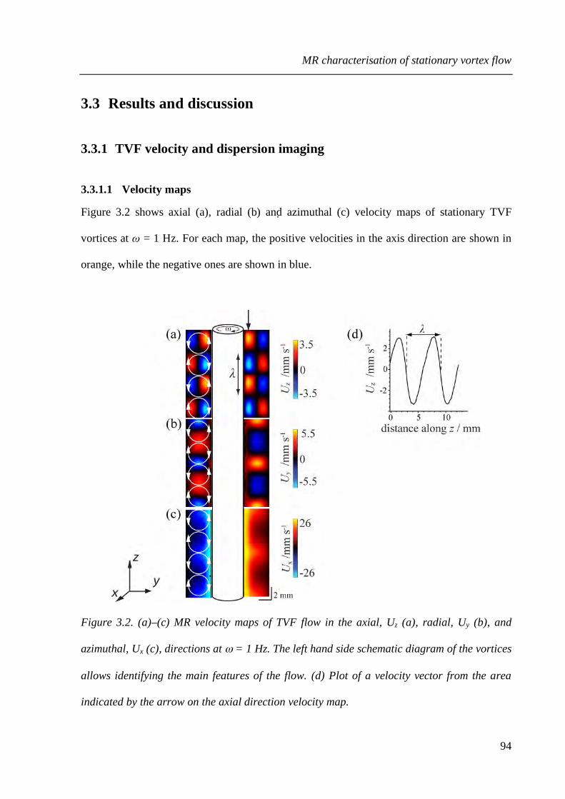
MR characterisation of stationary vortex flow

94

3.3 Results and discussion

3.3.1 TVF velocity and dispersion imaging

3.3.1.1 Velocity maps

Figure 3.2 shows axial (a), radial (b) and azimuthal (c) velocity maps of stationary TVF

vortices at ω = 1 Hz. For each map, the positive velocities in the axis direction are shown in

orange, while the negative ones are shown in blue.

Figure 3.2. (a)–(c) MR velocity maps of TVF flow in the axial, Uz (a), radial, Uy (b), and

azimuthal, Ux (c), directions at ω = 1 Hz. The left hand side schematic diagram of the vortices

allows identifying the main features of the flow. (d) Plot of a velocity vector from the area

indicated by the arrow on the axial direction velocity map.

MR characterisation of stationary vortex flow

95

Main structural features of TVF flow9 can be easily identified on these maps. The Uz map

shows the circulating motion of the vortices, with series of alternating positive and negative

velocities. In the inter-vortex regions the velocities in this direction are several times smaller

than in the vortex core revealing the low inter-vortex mixing properties of this flow. The

periodic variation of velocity with respect to space corresponds to the vortex pair wavelength.

Figure 3.2d shows how the plot of a velocity vector line allows measuring the wavelength.

The radial velocity map, Uy (Figure 3.2b), also highlights the vortex pair wavelength, with the

high positive velocities marking the outer edges of each vortex pair where the secondary flow

towards the outer cylinder is formed. This secondary flow appears in positive velocities on the

left hand side of the Couette gap, where the outflow is in the direction of the y-axis, and in

negative velocities on the left hand side. Velocities are positive all along the inner cylinder

side, with some pixels missing probably due to slight wobbling during the acquisition. The

Ux map (Figure 3.2c) shows velocities in-between vortex pairs that are an order of magnitude

higher compared to those inside the vortex pairs. Again, the velocities in the right hand side,

where the direction of rotation of the inner cylinder is the same as the direction of the x-axis,

appear in positive while the velocities in the left hand side appear in negative. The high radial

and azimuthal velocities in the outflow region of the vortex pairs dominate molecular

displacements. Their interplay with the vortical recirculation in the axial direction explains

the reduced inter-vortex exchanges observed at these regimes.

MR characterisation of stationary vortex flow

96

3.3.1.2 Diffusion/dispersion maps

Prior to the analysis of the diffusion/dispersion maps produced from the PGSE imaging

experiments it is important to understand the nature of the results obtained by the PGSE

sequence. The calculation of a diffusion/dispersion coefficient is based on the measurement of

the propagator broadening caused by phase spreading. This measurement is therefore very

sensitive to any effect that can introduce additional phase spread15. In the absence of flow,

and assuming that phase spread caused by the experimental setup and the spectrometer is

minimised, the phase spread arises mainly from Brownian motion. However, in most

propagator experiments presented in this thesis velocity shear is present in the system and

contributes to the phase spread measured during the PGSE experiment. This causes the

broadening of the propagator to be generated by both diffusion and velocity shear. In the case

of a PGSE imaging sequence this broadening is found to be proportional to velocity

differences between adjacent voxels16. This means that the dimension of the voxels will affect

the phase spread. Hence, despite the fact that the diffusion/dispersion maps allow to identify

regions of high and low dispersion, the quantitative nature of the coefficients obtained has to

be considered with precaution since they include the effects of flow inhomogeneities. In order

to measure only stochastic motion such as diffusion or dispersion in a system in the presence

of flow, and produce a quantitative diffusion or dispersion map, the voxel size would have to

be small enough so that the velocity shear contribution, caused by velocity inhomogeineities,

can be neglected. This is not always achievable, especially in systems were high shear is

present. An alternative method consists in exploiting the fact that, contrary to Brownian

motion, velocity shear is coherent and its effects can therefore be reversed using an

appropriate pulse sequence, such as the double PGSE pulse sequence17,18.

MR characterisation of stationary vortex flow

97

Figure 3.3 shows axial (d), radial (e) and azimuthal (f) diffusion/dispersion maps at the same

rotation rate as the velocity maps (ω = 1 Hz). Diffusion/dispersion maps for this flow have

not been previously reported in the literature.

Figure 3.3. (a)–(c) MR diffusion/dispersion maps of TVF flow in the axial, Dz (a), radial, Dy

(b), and azimuthal, Dx (c), directions at ω = 1 Hz. The observation time was of 20 ms. The left

hand side schematic diagram of the vortices allows identifying the main features of the flow.

(d) Plot of propagators for the positions A and B shown on the radial direction

diffusion/dispersion map.

The higher dispersion regions are identified close to the inner cylinder where the velocity

gradients are higher. Between vortex pairs, where the radial and azimuthal direction velocity

profiles are less sharp, reduced dispersion is observed. Despite the fact that it presents one

MR characterisation of stationary vortex flow

98

order of magnitude lower dispersion rates, the axial direction diffusion/dispersion map is of

particular interest, since it is linked with inter-vortex exchanges and can help us analyse axial

dispersion in the system. Note that a map of this system with a stable inner cylinder (no flow)

gives a uniform coefficient of 2 × 10−9 m2 s−1, in this case it can be called a diffusion map

since no dispersion effects are measured. The values obtained in the diffusion/dispersion

maps (Figure 3.3) are varying from 2 × 10−9 m2 s−1 to 70 × 10−9 m2 s−1 indicating the dominant

role of flow-induced dispersion in determining the molecular displacements measured.

The high dispersion regions in the axial direction (Figure 3.3a) are situated in the regions of

friction between the vortices’ higher velocities and the wall. The vortex core region, where

higher dispersion is observed, can be clearly seen in the middle of each vortex. Finally, in the

area between the vortex pairs, dispersion seems low, except from a point near the inner

cylinder, where high velocities of opposed direction are adjacent. In this region, enhanced

molecular exchanges between vortex pairs might be occurring. These results are in agreement

with previous studies19 showing higher inter-vortex mixing near the inner wall region and the

inflow boundaries. In the radial direction, the secondary flow generates additional dispersion

increase in between vortex pairs. For each pixel of the diffusion/dispersion maps a

propagator can be obtained by Fourier transformation of the signal decay against the gradient

increase. Figure 3.3d shows propagators from two pixels A and B shown in the radial

direction diffusion/dispersion map. These propagators give the probability distribution of

molecular displacements along the y-axis during the observation time Δ = 20 ms. The

propagators are centred around zero displacement, due to the fact that the velocities in both

regions are equal to zero. Coherent flow would lead to an offset of the propagator along the

displacement axis. In this case, the propagators are mainly affected by incoherent flow

MR characterisation of stationary vortex flow

99

(dispersion and self-diffusion). A wider propagator corresponds to a higher dispersion

coefficient within a given pixel. The width at the average height is equal to (4DyΔ)1/2, where

Dy is the average diffusion/dispersion coefficient. For low velocity gradient regions (B) the

propagator seems more affected by self-diffusion and is similar to a typical Gaussian

distribution of molecular displacements. The main difference is the presence of high

displacement side lobes. At higher velocity gradient regions (A), the shape of the propagator

is modified towards a more triangular shape, with a linear distribution of molecular

displacements. Finally, in the azimuthal direction (Figure 3.3c), the higher dispersion is

observed along the length of the vortex pairs, where the sharper velocity profiles in the

azimuthal direction are generated. High dispersion is also found in the region of the outer

cylinder where the secondary flow is formed.

3.3.2 The effect of rotation on TVF flow structure

The effect of ω on the flow within a Couette cell was investigated. The axial direction

velocity maps are shown in Figure 3.4. Below the critical rotation rate for the TVF instability

onset is applied, no coherent flow can be measured in the axial direction (Figure 3.4a).

Measurements show that the TVF instability arises at around 0.7 Hz. At ω = 1 Hz (Figure

3.4b), the series of alternating positive and negative velocities indicate the presence of

vortices stacked along the length of the cell. For this rotation rate range, the velocities

increase for increasing rotation rates, with the part of the vortices situated near the inner

cylinder presenting always higher velocities than the ones measured near the outer cylinder.

The opposed negative and positive velocities at the secondary flow regions are coming closer

as rotation increases, and the vortical regions close to the inner cylinder are expanding taking

MR characterisation of stationary vortex flow

100

more and more space in the gap centre (Figure 3.4c-d). Also, the interface between the

positive and negative regions is reduced before becoming unstable at ω = 2.5 Hz (Figure

3.4e).

Figure 3.4. Axial direction (z) velocity maps at increasing ω: (a) 0.5 Hz, (b) 1 Hz, (c) 1.5 Hz,

(d) 2 Hz and (e) 2.5 Hz. The rotating inner cylinder is situated on the left hand side of each

image.

In the radial direction, below the critical rotation rate (Figure 3.5a) a velocity gradient is

observed with the higher velocities close to the inner wall. Above the critical rotation rate

(Figure 3.5b-e) secondary flow can be observed in orange. This flow is always at higher

velocities than the inflow towards the inner cylinder (in blue). For low rotation rates, this

region is symmetric with respect to the y-axis (Figure 3.5b). As the rotation rate is increased,

both direction velocities are increased. The secondary flow velocity gradients are steeper and

the region situated near the rotating cylinder is narrower (Figure 3.5d-e). At ω = 2.5 Hz

(Figure 3.5e) the region corresponding to the secondary flow is unstable and not symmetric

with respect to the y-axis, indicating a possible state transition.

MR characterisation of stationary vortex flow

101

Figure 3.5. Radial direction (y) velocity maps at increasing ω: (a) 0.5 Hz, (b) 1 Hz, (c) 1.5

Hz, (d) 2 Hz and (e) 2.5 Hz. The rotating inner cylinder is situated on the left hand side of

each image.

The azimuthal direction velocity maps (Figure 3.6a-e) present the higher velocities. The

product between the rotation rate and the perimeter of the cylinder gives the velocity on the

inner cylinder. At ω = 0.5 Hz (Figure 3.6a) higher velocities are observed near the inner wall

but no instability is seen. As the rotation increases the velocity gradient between the rotation

inner cylinder and the stationary outer cylinder becomes steeper. This velocity gradient

generates an opposition between centrifugal forces towards the outer cylinder and pressure

gradients toward the inner cylinder. Above the critical rotation rate, secondary flow arises,

characterised by periodic velocity increases along the length of the cell (Figure 3.6b). The

outflow regions have less steep profiles in the radial direction than the neighbouring regions.

Further increase in rotation makes this secondary flow velocity profiles steeper, both in the

axial and radial direction. At ω = 2.5 Hz these regions become unstable and the system seems

to switch to wavy TVF9.

MR characterisation of stationary vortex flow

102

Figure 3.6. Azimuthal direction (x) velocity maps at increasing ω: (a) 0.5 Hz, (b) 1 Hz, (c) 1.5

Hz, (d) 2 Hz and (e) 2.5 Hz. The observation time was of 20ms. The rotating inner cylinder is

situated on the left hand side of each image.

Figure 3.7 shows a plot of the evolution of the maximum velocity for each direction against

the rotation rate. For all these experiments, the maximum velocities have been found to

increase linearly with the rotation rate. The non-slip boundary condition at the inner cylinder

surface allows to calculate the maximum velocities in this direction: Umax = 2πRiω ≈ 26ω. As

we see from the x direction plot this trend is found in our experimental data where Umax ≈

26ω. In the axial and radial directions, the maximum velocity increase with rotation follows a

linear trend of smaller slope (Umax ≈ 10ω in the y direction and Umax ≈ 5ω In the z direction).

The fact that the maximum velocities in the radial direction are two times higher than the ones

in the axial direction indicates that the circulation in the vortices is not done at uniform speed.

This is probably due to the presence of helical streamlines wrapping around the torroidal

vortices20.

MR characterisation of stationary vortex flow

103

Figure 3.7. Maximum velocities, Umax, against rotation rate for velocity maps in the azimuthal

(x), radial (y) and axial (z) direction.

One other important parameter that can be extracted from the velocity maps is the vortex pair

wavelength, λ. The spatial periodicity within this flow was measured by plotting velocity

vectors along the axial direction as shown previously (Figure 3.2d). Velocity vectors were

selected from the middle of the gap of the velocity maps. Figure 3.8 shows plots of the

measured wavelength in each direction, for different rotation rates. For low rotation rates,

similar wavelength is measured in every direction velocity map. For ω ≥ 2 Hz, there is more

spread in the measurements, and the wavelength in the azimuthal direction is found to be

shorter than the ones in the axial and radial directions. The wavelength in the axial direction is

also reduced at ω = 2.5 Hz, but in the radial direction the wavelength increases. As the

difference between wavelengths in different directions is increased, the shape of the vortices

is expected to change. The difference of wavelength between flow in different directions

might give information on the flow structure transition to wavy TVF and has to be further

investigated.

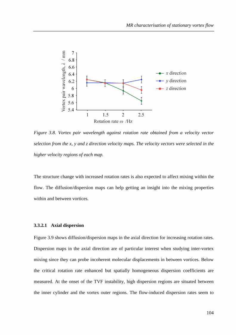
MR characterisation of stationary vortex flow

104

Figure 3.8. Vortex pair wavelength against rotation rate obtained from a velocity vector

selection from the x, y and z direction velocity maps. The velocity vectors were selected in the

higher velocity regions of each map.

The structure change with increased rotation rates is also expected to affect mixing within the

flow. The diffusion/dispersion maps can help getting an insight into the mixing properties

within and between vortices.

3.3.2.1 Axial dispersion

Figure 3.9 shows diffusion/dispersion maps in the axial direction for increasing rotation rates.

Dispersion maps in the axial direction are of particular interest when studying inter-vortex

mixing since they can probe incoherent molecular displacements in between vortices. Below

the critical rotation rate enhanced but spatially homogeneous dispersion coefficients are

measured. At the onset of the TVF instability, high dispersion regions are situated between

the inner cylinder and the vortex outer regions. The flow-induced dispersion rates seem to

MR characterisation of stationary vortex flow

105

increase rapidly with rotation rate until reaching an order of magnitude higher values for ω =

1.5 Hz. For ω ≥ 1.5 Hz, dispersion rate increase with rotation is less important, but there is a

more homogeneous distribution of high dispersion regions within the vortices. The region of

higher dispersion has now moved from the areas between the inner cylinder and the vortices

to the inter-vortex area where the secondary flow is directed towards the outer cylinder. That

is expected to increase intra-vortex relative to inter-vortex dispersion related mixing.

Figure 3.9. Axial direction (z) diffusion/dispersion maps at increasing ω: (a) 0.5 Hz, (b) 1 Hz,

(c) 1.5 Hz, (d) 2 Hz and (e) 2.5 Hz. The observation time was of 20 ms. The rotating inner

cylinder is situated on the left hand side of each image.

Note that the inter-vortex areas, where flow is coming towards the inner cylinder, maintain

low dispersion rates relative to the vortex centres, indicating poor dispersion induced inter-

vortex exchanges. This is in agreement with dye measurement studies showing that local

mixing intensity increase is not followed by similar axial dispersion increase21.

MR characterisation of stationary vortex flow

106

The analysis of velocity and diffusion/dispersion maps gives good insight into TVF flow

structure, but presents limitations when studying mixing. This is because it is not possible to

get a direct measure of intra or inter-vortex mixing using these maps. However, this

information could be gathered using bulk propagators measurements.

3.3.3 Molecular displacements and mixing in TVF

Figure 3.10 shows conditional probability of molecular displacement plots, propagators, for

TVF at ω = 1 Hz, over a range of observation times Δ. As expected, the maximum

displacement in P(Z, Δ) increases with increasing mixing time. The propagators are centred

about zero displacement with a symmetrical structure, consistent with flow recirculation in a

vortex pair. The peak at zero displacement reveals that a large number of molecules are not

moving along the z direction during this observation time. This peak corresponds to both

molecules of the outer wall and to molecules travelling perpendicular to the z direction, as the

ones that are caught by the strong inter-vortex velocities in the radial and azimuthal

directions.

Figure 3.10. Normalised propagators for TVF flow with ω = 1 Hz at increasing mixing times

Δ: 20ms (a), 100 ms (b), and 1 s (c). 64 q-slices and 4 averages were used for these

experiments.

MR characterisation of stationary vortex flow

107

The symmetry of the propagators with respect to zero displacements is showing that the flow

imposes even molecular displacements in both directions along the Couette cell axis. For

Δ = 20 ms (Figure 3.10), the propagators have a triangular shape. As the mixing time is

increased, the molecular displacements get more and more affected by the flow as molecules

have had the time to sample a greater area of the vortices. Small side lobes appearing for

Δ = 0.1 s are clearly formed at Δ = 1 s. These lobes correspond to high-circulation regions

within the flow and could possibly be linked with inter-vortex displacements16. This cannot

be verified experimentally at this regime because not enough molecules travel the distance of

a vortex in the z direction (≈ 3.1 mm) during 1 s. Molecular-displacement measurements at

higher observation times would have helped characterising inter-vortex mixing at this regime,

but MR relaxation limits PGSTE experiments to Δ ≤ 1 s. Nevertheless, the possibility to

distinguish high and low circulation zones is in adequacy with previously proposed models of

the TVF vortices16, where a low mixing vortex core and a high circulation outer zone are

considered.

For higher rotation rates the displacements where expected to cover the distance

corresponding to one vortex and help with the analysis of inter-vortex exchanges in the

system. Figure 3.11 shows propagators at Δ = 1 s for increasing rotation rates. Comparison

between propagators (ω = 1 Hz - Δ = 1 s) obtained with 64 q-slices / 4 averages (Figure

3.10a) and 128 q-slices / 16 averages (Figure 3.11a) shows that a higher number of q-slices

allowed for more details to be probed, but that the propagators lost their smooth shape. For ω

≥ 1.5 Hz (Figure 3.11b-d), the propagator side lobes are reduced and expand over more than

one vortex in both directions along z. The peak at zero displacement does not seem to change

a lot for ω = 1.5 Hz and ω = 2 Hz. At ω = 2.5 Hz the side lobes have almost disappeared and

MR characterisation of stationary vortex flow

108

the propagator starts having a triangular shape. The broadening of the central peak at this

rotation rate indicates a more homogeneous distribution of molecular displacements. This

homogenisation suggests a more uniform mixing within the vortices, and is in agreement with

the analysis of the diffusion/dispersion map results (Figure 3.9) where more homogeneous

dispersion coefficients were found in the vortex core region. These propagators allow to

quantitatively verify these results. Inter-vortex mixing can be estimated using the molecular

displacements that are found to exceed the vortex dimension (Figure 3.11).

Figure 3.11. Normalised propagators for TVF flow at Δ = 1 s for increasing rotation rates ω:

1 Hz (a), 1.5 Hz (b), 2 Hz (c) and 2.5 Hz (d). 128 q-slices and 16 averages were used for these

experiments. The distance between the doted lines correspond to one vortex pair wavelength.

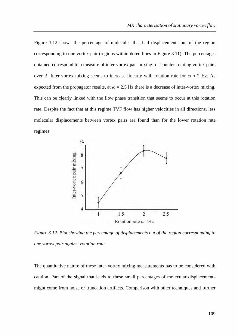
MR characterisation of stationary vortex flow

109

Figure 3.12 shows the percentage of molecules that had displacements out of the region

corresponding to one vortex pair (regions within doted lines in Figure 3.11). The percentages

obtained correspond to a measure of inter-vortex pair mixing for counter-rotating vortex pairs

over Δ. Inter-vortex mixing seems to increase linearly with rotation rate for ω ≤ 2 Hz. As

expected from the propagator results, at ω = 2.5 Hz there is a decrease of inter-vortex mixing.

This can be clearly linked with the flow phase transition that seems to occur at this rotation

rate. Despite the fact that at this regime TVF flow has higher velocities in all directions, less

molecular displacements between vortex pairs are found than for the lower rotation rate

regimes.

Figure 3.12. Plot showing the percentage of displacements out of the region corresponding to

one vortex pair against rotation rate.

The quantitative nature of these inter-vortex mixing measurements has to be considered with

caution. Part of the signal that leads to these small percentages of molecular displacements

might come from noise or truncation artifacts. Comparison with other techniques and further

MR characterisation of stationary vortex flow

110

experiments on reactors presenting higher inter-vortex mixing might help establishing this

technique providing with quantitative measurements of inter-vortex mixing.

3.4 Conclusions

Magnetic resonance techniques were used to characterise Taylor vortex flow. The

combination of MR velocity and diffusion/dispersion mapping with propagator measurements

was shown to provide with means, not only to characterise velocity and dispersion fields, but

also to obtain quantitative information on micro-mixing within the studied flows.

Velocity maps of TVF in all directions helped analysing the structure of TVF flow and

identify how the interplay between velocity fields can produce the stationary vortex structure.

Velocities in all direction were shown to depend linearly on the rotation rate. Critical rotation

rates for the onset of the instability (0.5 Hz < ω < 1 Hz) and transition to unsteady TVF

regimes (2 Hz < ω < 2.5 Hz) were determined. At these unsteady regime, the vortex-pair

wavelength was found to vary in the different directions, providing with possible explanations

so as to the nature of the transition. The first produced diffusion/dispersion maps of TVF in

all directions gave an insight into the dispersion properties of the flow. As rotation was

increased a more uniform diffusion/dispersion coefficient in the vortex core was identified,

probably related to better intra-vortex mixing.

Propagator experiments were shown to address the limitations of velocity and

diffusion/dispersion mapping in characterising micro-mixing within TVF. Propagators were

shown to provide with insight into both intra and inter-vortex mixing. Low and high

MR characterisation of stationary vortex flow

111

displacement molecular paths within the vortices were identified, supporting a two-zone

model for the analysis of TVF. Quantitative inter-vortex mixing measurements were provided

for increasing rotation rates. For the laminar TVF regimes in this system (ω ≤ 2 Hz) inter-

vortex mixing increased linearly while the TVF regime change that occurs at ω = 2.5 Hz is

followed by an increase of intra-vortex mixing and a decrease of inter-vortex mixing. Note

that propagator experiments overcome the limitations of MR imaging at high Ta numbers

(unsteady and turbulent flows), allowing probing molecular displacements at all flow regimes

within a Couette cell. Although the quantitative nature of these measurements has to be

confirmed by future studies, the ability of propagators to probe mixing in vortical flow is

indubitable.

(1) Kataoka, K.; Ohmura, N.; Kouzu, M.; Simamura, Y.; Okubo, M. Chem. Eng.

Sci. 1995, 50, 1409.

(2) Holeschovsky, U. B.; Cooney, C. L. AIChE J. 1991, 37, 1219.

(3) Haut, B.; Ben Amor, H.; Coulon, L.; Jacquet, A.; Halloin, V. Chem. Eng. Sci.

2003, 58, 777.

(4) Ameer, G. A.; Grovender, E. A.; Obradovic, B.; Cooney, C. L.; Langer, R.

AIChE J. 1999, 45, 633.

(5) Hill, E. K.; Krebs, B.; Goodall, D. G.; Howlett, G. J.; Dunstan, D. E.

Biomacromolecules 2006, 7, 10.

(6) Tagg, R. A Guide to Literature Related to the Taylor-Couette Problem. In

Ordered and Turbulent Patterns in Taylor-Couette Flow; Andereck, C. D., Hayot, F., Eds.;

Springer US, 1992; pp 303.

(7) Kose, K. Phys. Rev. Lett. 1994, 72, 1467.

MR characterisation of stationary vortex flow

112

(8) Seymour, J. D.; Manz, B.; Callaghan, P. T. Phys. Fluids 1999, 11, 1104.

(9) Koschmieder, E. L. Bénard cells and Taylor vortices; Cambridge University

Press: Cambridge [England] ; New York, 1993.

(10) Elkins, C. J.; Alley, M. T. Experiments in Fluids 2007, 43, 823.

(11) Packer, K. J.; Stapf, S.; Tessier, J. J.; Damion, R. A. Magn. Reson. Imaging

1998, 16, 463.

(12) Waggoner, R. A.; Fukushima, E. Magn. Reson. Imaging 1996, 14, 1085.

(13) Kutsovsky, Y. E.; Scriven, L. E.; Davis, H. T.; Hammer, B. E. Phys. Fluids

1996, 8, 863.

(14) Seymour, J. D.; Callaghan, P. T. AIChE J. 1997, 43, 2096.

(15) Callaghan, P. T.; Trotter, C. M.; Jolley, K. W. J. Magn. Res. 1980, 37, 247.

(16) Xia, Y.; Callaghan, P. T. J. Magn. Res. 1991, 91, 326.

(17) Khrapitchev, A. A.; Callaghan, P. T. J. Magn. Res. 2003, 21, 373.

(18) Callaghan, P.-T. Translational dynamics and magnetic resonance : principles

of pulsed gradient spin echo NMR; Oxford University Press, 2011.

(19) Dusting, J.; Balabani, S. Chem. Eng. Sci. 2009, 64, 3103.

(20) Desmet, G.; Verelst, H.; Baron, G. V. Chem. Eng. Sci. 1996, 51, 1287.

(21) Desmet, G.; Verelst, H.; Baron, G. V. Chem. Eng. Sci. 1996, 51, 1299.

MR characterisation of translating vortex flow

113

4 MR characterisation of translating vortex flow

4.1 Introduction

The combination of MR velocity and diffusion/dispersion mapping with MR propagator

measurements was shown to provide with rich information on the stationary Taylor vortex

flow (TVF). This section expands this approach to the translating vortex flow produced in a

Vortex Flow Reactor (VFR). A VFR is obtained by superimposing pipe flow on steady Taylor

Vortex Flow. The resulting flow consists of a series of counter-rotating vortex pairs travelling

along the length of the Couette cell. Plug flow properties and non-agitative mixing inside the

translating vortices make the axi-symmetric, laminar flow regime of a VFR an ideal candidate

for numerous chemical1−3 and biochemical4,5 applications. However, the literature reveals that

open questions still remain for important flow properties as inter-vortex and intra-vortex

mixing. In particular, the emergence of by-pass flow, where fluid is able to flow at a different

velocity to the translating vortices, is a topic of much debate6,7. One of the most commonly

used parameters for the analysis of the VFR flow properties is the velocity drift, Vd, given by

the ratio of the translation velocity of the vortices, UTV, to the axial flow average velocity,

Uax.

!

Vd =UTV

Uax

( 4.1 )

Several authors have assumed that Vd = 1 in order to support the “translating tanks” model for

the flow, where the VFR is considered to be ideal an plug flow reactor6,8,9. This assumption

has been widely adopted despite a growing literature highlighting its inaccuracy in many

systems10−12, where the velocity drift is found to vary from 1 to 1.4. Desmet et al.13,14

MR characterisation of translating vortex flow

114

demonstrated the existence of a significant inter-vortex flux for the stationary vortices, which

refutes the generally-accepted concept of zero intermixing between vortex units. These results

also further questioned the plug-flow hypothesis for a VFR. Later, Giordano et al.7 showed

that, by increasing ω, it is possible to decrease the velocity of the Taylor vortices until

obtaining stacked vortices with a flow passing through them. In their experiments, Vd was

found to vary between 0 and 1. Haim and Pismen11 considered the role of the strong

secondary flow in transforming pipe flow into a slalom by-pass around the vortices that could

be completely suppressed at higher rotation rates. Giordano et al.7,15 used this model to

explain how an increase in rotation could decrease UTV by increasing the by-pass flow. VFR

models developed after this work were suitable for dealing with the by-pass flow4,16. In 1999,

Wereley et al.12, by removing the pressure driven axial velocity field from the overall velocity

field in their VFR, obtained a flow field very similar to the linear TVF one. Their results

suggest that VFR flow could be a linear superposition of pipe flow and TVF. These results, in

addition with studies demonstrating that vortical flows can generate Levy flights and resonant

mixing, are revealing the limitations of the translating tank and by-pass models in addressing

the flow complexity. A new understanding of VFR flow is necessary in order to reflect the

dependence of the mixing properties on the system parameters and the role of Vd in

characterising flow properties.

MRI velocity and diffusion/dispersion maps of this flow could provide answers for these

questions, but the VFR flow has properties that make it difficult to image. The main challenge

lies in the periodic motion of the translating vortices, causing imaging artifacts and errors in

velocity measurements. Periodic flow makes pixel signal magnitude and/or phase to change

during motion encoding and acquisition, leading to inconsistencies between acquisitions17. An

MR characterisation of translating vortex flow

115

increase in phase dispersion inside voxels can lead to multi-lobe propagators generating

velocity disparities inside pixels and errors in the velocity calculation17. Phase-encoding is

more affected by velocity field fluctuations18. If the motion is periodic, artifacts appear as

discrete replicates (ghosts) of the moving structures. In the case of periodically fluctuating

Poiseuille flow19, the amplitude of ghosts has been shown to increase with the amplitude and

frequency of the fluctuations but also with several imaging parameters (δ, Δ, g). On the other

hand, a repetition time increase leads to a ghost intensity reduction. Most common approaches

to reduce artifacts consist in reducing δ, Δ and g. By decreasing the pixel size it is also

possible to avoid big velocity ranges within spins in each voxel, but this necessitates a

gradient increase that is also source of artifacts. Finally, the reduction of amplitude and

frequency of velocity fluctuations in the sample is also reducing the observed artifacts. In the

case of VFR flow this will consist in working at lower rotation and flow rates.

Previous attempts to characterise VFR flow using MRI by Moser et al.20, have relied on a 2D

imaging method combining DANTE spatial tagging with a fast imaging sequence. The

vortical structure within the VFR was identified and the translation velocity UTV was

measured. However, these measurements were not able to provide 3D characterisation of the

flow and the images were restricted to low resolution, in order to reduce the imaging time and

hence artifacts. Producing high-resolution 3D images in a VFR requires longer experimental

times and/or faster imaging sequences.

In this study, in order to remove the effects of periodic flow, the PGSE imaging sequence was

synchronised with the flow period, TTV. Data was acquired when the successive vortices were

at the same spatial point. A similar method was successfully employed by Han et al.21 who

MR characterisation of translating vortex flow

116

mapped the velocity of fluid inside a falling droplet by gating the acquisitions to the droplet

dispenser. Unlike their system, VFR flow is continuous and TTV is not a directly controllable

parameter. Hence, optical experiments using dye visualisation were performed on the VFR

system in order to measure the flow periodicity at different flow and rotation ranges. These

measurements were also used for comparison with the existing literature and for helping with

the analysis of the MR data.

MR velocity imaging using a pulse sequence timed to the flow period allowed producing the

first three-dimensional velocity maps of the VFR flow22. These velocity maps are used to

characterise the velocity field structure and get a better understanding of the respective roles

of axial and TVF flow in the resulting VFR flow. Maps obtained by superposition of axial and

TVF flow velocity maps were compared with VFR maps in order to test the linear

superposition hypothesis12. The role of Vd in characterising the plug flow properties of the

reactor is discussed.

Finally, molecular transport in pipe flow, TVF and VFR flow was investigated by performing

propagator measurements. The propagator analysis is shown to provide with quantitative

information on molecular mixing within these systems. The effect on mixing of each of the

two superposed flows (axial and TVF) that form the VFR flow is discussed. The effects of

rotation and flow rate on molecular displacement within a VFR are investigated.

MR characterisation of translating vortex flow

117

4.2 Experimental

4.2.1 Vortex Flow Reactor dimensions and set-up

The Couette cell used in this study is the same as the one used for the TVF studies (Chapter

3). The VFR reactor (Figure 4.1) was obtained by superimposing pipe flow to the TVF and

constructed from an outer glass tube of radius Ro = 8.25 mm and an inner PEEK rod of radius

Ri = 4.1 mm, resulting in a gap, d, of 4.15 mm.

Figure 4.1. Schematic diagram of the VFR. The arrows show the flow circulation within the

system. The area within the rf coil corresponds to the field of view for both dye and MR

experiments.

MR characterisation of translating vortex flow

118

The effective length of the Couette cell, L, was of 896 mm, giving a length to gap ratio Γ of

216 and a radius ratio η of 0.5. PTFE guides were placed at the top and bottom of the cell, to

reduce wobble from the inner cylinder. The inner cylinder was rotated using a stepper motor

(Bruker NMR Rheokit). The connection between the motor and the inner cylinder was made

with a rubber connection absorbing vibration transmission and shocks due to alignment

errors. The VFR was placed in the magnet with the MRI field of view of the rf coil situated

11 cm above the lower inner cylinder guide. An Ismatec pump was used to pump solution

through the VFR. A pulsation reducer was placed at the pump outlet in order to reduce the

pump pulse effects.

In previous VFR studies7,9,10,12,20,23−29, η was found to vary between 0.5 and 0.9, and Γ

between 12 and 120. The VFR used in this work has one of the smallest radius ratios in the

literature and the larger characteristic length. This is mainly due to the constraints linked with

MR imaging: the VFR had to be thin enough to fit the in the probe and long enough to

connect the stepper motor at the top and the pump at the bottom. To avoid the unsteady wavy

vortex regimes, both for better MR results and for ensuring better plug-flow properties, a

large gap VFR was used30, leading to a small radius ratio η.

4.2.2 Parameter ranges

Tap water was used for all the experiments presented in this chapter. The viscosity ν,

measured with a calibrated Ubbelohde viscometer, was of 0.979 mm2 s−1 at 22 ± 0.5 ˚C. Five

evenly spaced rotation rate values, ω, were used, from 1 Hz to 2.5 Hz. The respective Ta

values varied from 17 to 42.5. Four flow rate values, Q, were used: 4 cm3 min−1, 7.2 cm3 min−

MR characterisation of translating vortex flow

119

1, 10.4 cm3 min−1 and 13.6 cm3 min−1. The respective Re values varied from 1.7 to 5.3 and γRe

= Uax / Riω varied from 0.03 to 0.29. The velocity of translation of the vortices varied

between 0.45 mm s-1 and 1.51 mm s-1 and the velocity drift, Vd, between 1.02 and 1.21.

Measurements were performed 5 min after setting the rotation and flow rates. Each

experiment was repeated a minimum of three times.

4.2.3 Optical and timing measurements

Optical images were acquired using a digital CCD camera Canon EOS 1000 and transferred

to a PC using the remote capture utility of the EOS software. To follow the evolution of the

system over time, images were acquired every 5 s using the remote control option of the

software.

The visualisation of the vortices was done by injecting 0.2 ml of a dye (ferroin solution,

[ferroin] = 3.74 mM) with a syringe at the inlet of the pump. The vortex pair wavelength, λ,

was measured on photographic material. Each value of λ corresponds to an average over a

minimum of three measurements. The speed of the translating vortices, UTV, was obtained by

measuring the time t taken by the vortices to travel a given distance. The time necessary for

one vortex pair to travel one wavelength corresponds to the flow period, TTV. The velocity

drift, Vd, is given by the ratio of Taylor vortices velocity, UTV, to the axial average velocity,

Uax. The value deviation was of 5%. All optical measurements were taken for the region of

the Couette cell that was positioned inside the rf coil in the MR measurements.

MR characterisation of translating vortex flow

120

4.2.4 Velocity imaging of steady flow

A Pulsed Gradient Spin Echo (PGSE) velocity imaging sequence was used (Figure 2.15). The

PGSE parameters used for these experiments were in the following ranges: Δ = 10 - 30 ms, δ

= 1 - 2 ms and G = 0.1 - 0.6 T m−1. The hard 90° excitation pulse was typically of 43-45 µs. A

soft 180° Gaussian pulse of 1000 µs was used for slice selection, with an attenuation range of

16 - 16.8 dB. A slice thickness of 1 mm was used, with a field of view of 50 × 25 mm and a

matrix size of 256 × 128 pixels resulting in a pixel size of 0.196 × 0.196 mm. The spectral

width was of 100 kHz. 4 q-slices were acquired with 2 signal averages.

4.2.5 Velocity imaging of periodic flow

For velocity imaging of periodic flow most PGSE and imaging sequence parameters were

similar to the steady flow experiments. Phase pixels were reduced to 64 pixels giving a matrix

size of 256 × 64 pixels. Also, the field of view was reduced to 40 × 20 mm, resulting in a

pixels size of 0.156 × 0.313 mm. The three loops defining the PGSE pulse sequence were

adapted to the flow period (TTV) (Figure 4.2): the acquisition loop, repeated 64 times (nph

phase points) to acquire all the blocks of time domain size, the experiment average loop (navg

averages), repeated twice and the gradient encoding loop (nq q-slices), repeated 2 or 8 times

depending on the experiment. Flow and rotation rate were kept constant and series of 2 q-slice

experiments were performed, varying the loop period by 20 ms steps. The period range was

defined by the experimental TTV values obtained by optical measurements. The loop time

varied from TTV – 500ms to TTV + 500ms. For each one of the imaging series with increasing

TTV, one single measurement was giving an intensity map with no appearing artifacts (no

MR characterisation of translating vortex flow

121

signal outside the gap region and no signal loss inside the gap region). The data acquired

during this measurement were post-treated to produce a velocity map of the measured flow.

Figure 4.2. The 3 loops defining the PGSE pulse sequence had to be adapted to the period of

the translating vortices (TTV).

4.2.6 Propagator measurements

A Pulsed Gradient Stimulated Spin Echo (PGSTE) sequence was used for the propagator

measurements31 (Figure 2.14). Either 64 or 128 q-steps were collected with 4 and 16 averages

respectively. The PGSTE parameters used were in the following ranges: Δ = 20 - 1000 ms, δ

= 1 - 2 ms and G = -0.6 - 0.6 T m−1.

MR characterisation of translating vortex flow

122

4.3 Results and discussion

4.3.1 Optical visualisation of travelling vortices

Dye injection experiments allowed a clear identification of the vortical structures in VFR

flow. Figure 4.3 shows of photos taken in the region of the VFR that contained the rf coil

during the MR experiments.

Figure 4.3. (a) Photographs of translating vortices in a 10 cm region of the VFR system at ω

= 1 Hz and Q = 7.2 cm3 min–1. Photographs were taken with an interval of 5 s. Vortices are

visualised using ferroin. (b) Close-up of the region highlighted in the doted square with a

schematic of the counter-rotating vortices.

Figure 4.3a shows time series of the propagation of the dye front. The dye spreads over

several vortex pairs, with the major part concentrated in 4 vortex pairs. This spread of the dye

into successive vortices gives insight into the by-pass and drag properties of the flow, where

molecules go faster or slower than the translating vortices. Figure 4.3b shows a close-up of

MR characterisation of translating vortex flow

123

the propagation front. The schematic of the vortex pairs allows understanding the observed

dye distribution. Each vortex pair is formed of two counter-rotating vortices separated by

secondary flow in the radial direction. For one over two vortices the outer part is colourless

while the core remains red, suggesting a heterogeneous dye distribution into successive

vortices. At the rear part of the high concentration dye region (Figure 4.3a(v)) the vortex

cores are colourless and the inter-vortex areas red. This indicates that the drag within this flow

is mainly occurring within the inter-vortex and outer-vortex areas.

Figure 4.4 shows plots of the measured wavelength, λ, against flow and rotation rate.

Figure 4.4. Plots of vortex pair wavelength against flow rate (a) and rotation rate (b).

MR characterisation of translating vortex flow

124

λ varied between 8.16 mm and 9.33 mm, but no clear trend with the experiment parameters

could be identified, except the fact that higher rotation and flow rates systematically lead to a

bigger spread of λ values. These results are close to the “square vortices” approximation, λ =

2d, often made in literature12,15 since 1.96d < λ < 2.25d, where d is the gap between the inner

and outer cylinder.

Figure 4.5 shows plots of UTV and TTV against flow rate at different rotation rates. At this

range, UTV is found to increase linearly with the flow rate, while TTV is decreasing. The rate of

decrease of TTV is higher for lower flow rates.

Figure 4.5. Plots of vortex translation velocity (a) and flow period (b) against flow rate.

Figure 4.6 shows plots of UTV and TTV against rotation rate for different flow rates. For Q > 4

cm3 min−1, UTV is found to decrease linearly and TTV to increase with rotation rate. These

results are in agreement with previous works where an increase in rotation rate was shown to

decrease the translation velocity of the vortices7. A different behaviour is observed only for

the lower flow rate (4 cm3 min−1) at high rotation rates, where UTV is increasing and TTV is

decreasing. Imposed pipe flow has been shown to delay the onset of the Taylor vortex

MR characterisation of translating vortex flow

125

instability and to stabilise the flow12, but below a critical flow rate the instable regime

observed at high rotation rates in TVF without axial flow (ω = 2.5 Hz) is expected to appear

(ref. chapter 3). These results suggest that 4 cm3 min−1 is below this critical flow rate.

Figure 4.6. Plots of vortex translation velocity (a) and flow period (b) against rotation rate.

To evaluate the velocity drift, Vd, and understand the importance of the pipe flow into the

resulting VFR flow, pipe flow was investigated using MR velocity imaging.

4.3.2 Pipe flow properties

Figure 4.7a shows a velocity map in the z-axis direction of pipe flow in the Couette cell with

stationary inner cylinder, at Q = 7.2 cm3 min−1. The dark part in the middle of the image

corresponds to the inner cylinder. An average over 50 cross-section lines of this velocity map

shows the typical Poiseuille velocity profile (Figure 4.7b). Due to the shape of the Couette

cell, the maximum velocities on the profile are found closer to the inner than the outer

cylinder32. The inner surface of the outer cylinder being larger than the surface of the inner

cylinder, higher friction is experienced on the outer side. The right-hand part of the velocity

MR characterisation of translating vortex flow

126

profile is slightly higher than the left hand-side. This symmetry break, probably caused by

inhomogeneous distribution at the inlet or a gap irregularity, has to be considered when

studying the VFR flow.

Figure 4.7. (a) Velocity map in the z direction of pipe flow at Q =7.2 cm3 min−1. (b) Average

velocity profile in the radial direction.

Figure 4.8 shows a plot of average (Uax) and maximum (Umax) velocities for different flow

rates. As expected, there is a linear relation between the average velocity and the pump flow

rate. Due to the Couette cell shape, the measured pipe flow profile is lying between Poiseuille

profile in a tube and Poiseuille profile between two parallel planes32. For low radii ratio, η,

the Couette cell looks more like a tube where typically Uax = 1/2 Umax, while for high η values

the TC cell gap is similar to the gap between two parallel planes where Uax = 2/3 Umax. So, the

ratio Uax / Umax is characteristic of each VFR device. In these results, Uax / Umax is found to be

constant at 0.64 ± 1 (Note that 1/2 < 0.64 < 2/3).

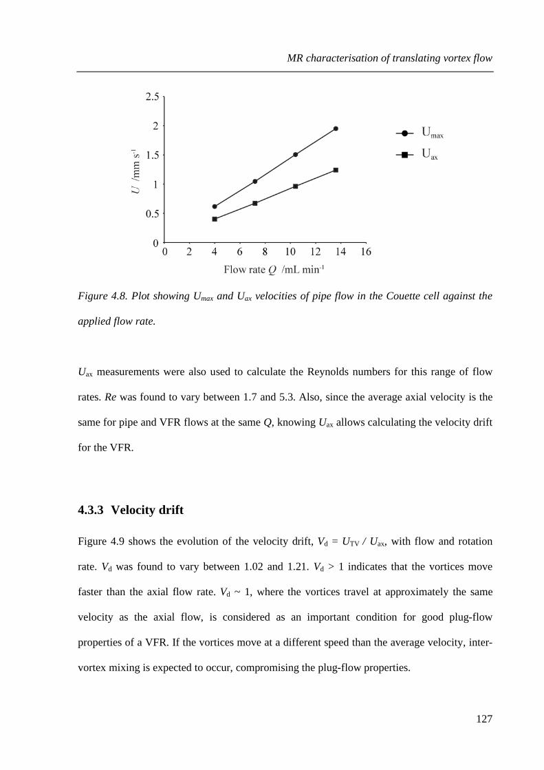
MR characterisation of translating vortex flow

127

Figure 4.8. Plot showing Umax and Uax velocities of pipe flow in the Couette cell against the

applied flow rate.

Uax measurements were also used to calculate the Reynolds numbers for this range of flow

rates. Re was found to vary between 1.7 and 5.3. Also, since the average axial velocity is the

same for pipe and VFR flows at the same Q, knowing Uax allows calculating the velocity drift

for the VFR.

4.3.3 Velocity drift

Figure 4.9 shows the evolution of the velocity drift, Vd = UTV / Uax, with flow and rotation

rate. Vd was found to vary between 1.02 and 1.21. Vd > 1 indicates that the vortices move

faster than the axial flow rate. Vd ~ 1, where the vortices travel at approximately the same

velocity as the axial flow, is considered as an important condition for good plug-flow

properties of a VFR. If the vortices move at a different speed than the average velocity, inter-

vortex mixing is expected to occur, compromising the plug-flow properties.

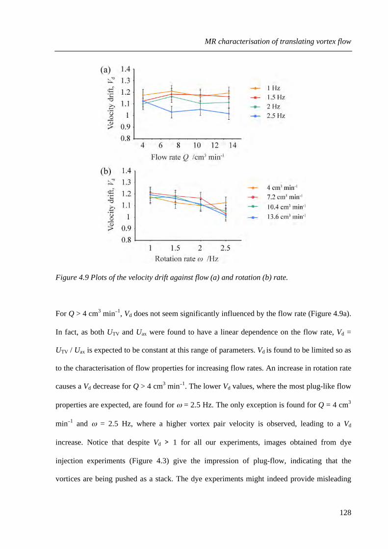
MR characterisation of translating vortex flow

128

Figure 4.9 Plots of the velocity drift against flow (a) and rotation (b) rate.

For Q > 4 cm3 min−1, Vd does not seem significantly influenced by the flow rate (Figure 4.9a).

In fact, as both UTV and Uax were found to have a linear dependence on the flow rate, Vd =

UTV / Uax is expected to be constant at this range of parameters. Vd is found to be limited so as

to the characterisation of flow properties for increasing flow rates. An increase in rotation rate

causes a Vd decrease for Q > 4 cm3 min−1. The lower Vd values, where the most plug-like flow

properties are expected, are found for ω = 2.5 Hz. The only exception is found for Q = 4 cm3

min−1 and ω = 2.5 Hz, where a higher vortex pair velocity is observed, leading to a Vd

increase. Notice that despite Vd > 1 for all our experiments, images obtained from dye

injection experiments (Figure 4.3) give the impression of plug-flow, indicating that the

vortices are being pushed as a stack. The dye experiments might indeed provide misleading

MR characterisation of translating vortex flow

129

information about the properties of the reactor. MR velocity imaging was performed to get a

better understanding of the VFR system.

4.3.4 MR Velocity imaging of travelling vortices

The travelling vortex period values, TTV, measured in the dye experiments (Figure 4.5 and

Figure 4.6) were used to time the PGSE velocity imaging sequence. Series of 2 q-slice MR

experiments were performed, where the triggering time of the pulse sequence varied from TTV

– 500ms to TTV + 500ms, with 20 ms steps. The experimental time for each image acquired

was of 18 to 40 minutes, depending on TTV. Figure 4.10 shows intensity maps obtained at

different loop time periods.

Figure 4.10. Intensity maps of VFR flow at ω = 1 Hz and Q = 7.2 cm3 min−1, obtained at

different PGSE loop times. The loop that eliminated artifacts had a period of 8.16 s (= TTV).

When the loop period of the sequence is different from TTV ± 20ms, several phase artifacts are

observed, with high signal observed in the region corresponding to the inner cylinder and low

signal regions in the gap area. This behaviour was observed for all direction experiments on

this VFR. As the PGSE loop period is approaching the estimated TTV value, less artifacts

appear on the intensity maps. For each one of the imaging series, only one measurement gives

MR characterisation of translating vortex flow

130

an intensity map with no apparant artifacts (no signal outside the gap region and no signal

loss inside the gap region). The loop time producing this intensity map corresponds to TTV.

Similar experiments were conducted on a second VFR, giving the same results (Appendix A).

The data acquired during this measurement were post-treated to produce a velocity map of the

measured flow.

Figure 4.11 shows axial (b), radial (c) and azimuthal (d) MR velocity maps at ω = 1 Hz and Q

= 7.2 cm3 min−1, in comparison with a dye visualisation picture at the same regime (a). The

vortex pair wavelength measured on the velocity maps is in agreement with the dye

experiment results (λ ∼ 85 mm). These velocity maps present also several similar features

with the TVF velocity maps at ω = 1 Hz (cf. 3.3.1). In fact, the addition of pipe flow does not

seem to have a strong effect on the velocity field. The velocity map in the direction of the

translating vortices, Uz, is more affected, since pipe flow does not have radial and azimuthal

components at this range. Figure 4.10b shows a slalom-like, high-velocity region, suggesting

the presence of by-pass flow. The higher velocities in the axial direction are found in the parts

of the vortices situated close to the inner cylinder. This can be explained by the fact that both

TVF and pipe flow exhibit enhanced velocities in this region. The radial direction velocity

map shows the secondary flow jets towards the outer cylinder.

MR characterisation of translating vortex flow

131

Figure 4.11. (a) Digital photo of translating vortices in the VFR system at ω = 1 Hz and Q =

7.2 cm3 min–1. (b)–(d) MR velocity maps of VFR flow in the axial, Uz (b), radial, Uy (c) and

azimuthal, Ux (d), directions.

These jets are not oriented perpendicularly to the inner cylinder as for TVF. The outer part of

the jet (on the outer cylinder) is positioned slightly lower than the inner part. This “bending”

MR characterisation of translating vortex flow

132

of the secondary flow is probably due to the higher axial velocities found close to the inner

cylinder. As with TVF, velocities in-between vortex pairs in the azimuthal direction (Figure

4.10d) are an order of magnitude higher compared to those inside the vortex pairs, so they are

not noticeably deformed. These strong inter-vortex flows, in combination with the periodic

outwards flow structures in the radial direction, create the sharp interfaces observed in the

dye-injection experiments. Despite the fact that the vortices move faster than the average axial

velocity (Vd ~ 1.2) and the observed high-velocity slalom-like region in the axial direction

velocity maps, these interfaces give the misleading impression of plug-flow, where vortices

appear as non inter-mixing translating reactors.

To compare with other studies of travelling vortex flow in a VFR, several approaches can be

used. A contour plot obtained using the axial direction map (Figure 4.12a) allows better

comparison with contour plots found in theoretical studies of the travelling vortex flow,

where streamlines are found to slalom around the vortex cores33. A 2D velocity vector map,

produced using the MR velocity maps (Figure 4.12b), facilitates comparison with particle

imaging velocimetry measurements12, typically used to study this flow. Moreover, a 2D map

can give a better visualisation of the vortical structures within a VFR. In this map, the MR

velocity maps (Uz and Uy) were used to define the magnitude of each vector in the axial and

radial directions. In the resulting 2D velocity vector map, the centre of the successive vortices

can be easily identified, as well as the slight distortions caused by the secondary inflows and

outflows in the radial direction.

MR characterisation of translating vortex flow

133

Figure 4.12. (a) Contour representation of the left part of the axial direction velocity map

(Uz) and (b) 2D velocity vector map obtained by combining the axial and radial direction

velocity maps.

MR experiments using 8 q-slices were also performed to obtain more accurate measurements.

The experimental time for each image to be acquired with the pulse sequence timed to the

flow period was of 2 - 3 hours. The main challenge in performing these experiments was to

maintain the vortex translation stable over the course of the 8 q-slice experiments. As

mentioned before, the precision required for the data synchronisation to eliminate motion

artifacts was of the order of 20 ms, and small axial flow rate variations (of the order of 0.05

cm3 min−1) tended to desynchronise the pulse sequence timing, resulting in motion artifacts.

Figure 4.13 shows a velocity map of VFR flow in the axial direction obtained with an 8 q-

MR characterisation of translating vortex flow

134

slice PGSE experiment. Artifacts can be noticed outside the gap (right-hand side) but also in

the inter-vortex regions where opposed direction velocities are found.

Figure 4.13. MR velocity map of VFR flow (at ω = 1 Hz and Q = 7.2 cm3 min-1) in the axial

direction obtained with an 8 q-slice PGSE experiment.

Despite the vortical shape being clearly identifiable and the wavelength in agreement with the

2 q-slice experiments, the overall velocities are found to be much lower, probably due to

disparities in the successive slices. Hence, 2 q-slice experiments were used to study the

relative effects of pipe flow and TVF in the resulting VFR flow.

4.3.5 VFR flow as a superposition between pipe flow and TVF

VFR flow is obtained by imposing pipe flow to TVF. As discussed earlier, several authors

assumed that the introduction of pipe flow was simply causing the vortices to translate along

the length of the reactor6. But the slalom high-velocity regions on the axial direction velocity

maps in a VFR (Figure 4.11b) show that the vortices are not simply "pushed" by the addition

MR characterisation of translating vortex flow

135

of pipe flow. In fact, the velocity field in a VFR appears as a combination between the

velocity fields of TVF and pipe flow. These results seem to support the assumption made by

Wereley et al.12, that the VFR velocity field could be modelled by an addition of pipe flow

and TVF velocity fields. MRI maps offer a simple way of testing this hypothesis, since model

VFR maps can be obtained by a pixel-to-pixel addition of pipe flow and TVF velocity maps.

Figure 4.14 shows experimental and modelled VFR velocity maps at the same flow and

rotation rates.

Figure 4.14. (a) Axial velocity map obtained by linear addition of experimental pipe flow (Q

=7.2 cm3 min–1) and TVF (ω =1 Hz) velocity maps. (b) Experimental velocity map of VFR

flow at ω =1 Hz and Q = 7.2 cm3 min–1. (c) Axial velocity map obtained by linear addition of

experimental pipe flow (Q =13.6 cm3 min–1) and TVF (ω =1 Hz) velocity maps. (d)

Experimental velocity maps of VFR flow at ω =1 Hz and Q =13.6 cm3 min–1.

The velocity maps obtained by linear addition show good agreement with the experimental

VFR flow ones. The main difference is that the model velocity maps have about 30% higher

velocities. Also, by removing the average axial map from the experimental VFR map one

MR characterisation of translating vortex flow

136

obtains a typical TVF map corresponding to a lower rotation rate12. This could be explained

by head loss occurring via the combination of the two flows. The strong TVF flow in

azimuthal direction possibly transforms a part of the coherent motion in the z direction into

dispersion, not detected by the velocity mapping experiments. Decrease in velocity in the

VFR maps is in agreement with experimental results12 showing that the addition of pipe flow

increases the critical rotation rate necessary for the formation of the vortices. Also, this

phenomenon could explain the possibility of stopping the moving vortices by increasing the

rotation rate7.

The properties of the slalom high-velocity region seem closely related to the pipe flow

properties. Comparison between VFR velocity maps at Q = 7.2 cm3 min−1 (Figure 4.14b) and

Q = 13.6 cm3 min−1 (Figure 4.14d) shows that for higher flow rates, this region is increased.

However, the velocity drift, Vd, typically used for analysing the VFR flow properties, was

found to be constant for all flow rates at a given rotation rate. These results highlight the

limitation of Vd in characterising flow properties in a VFR and in particular the presence and

properties of the slalom velocity region. The results presented here, could allow identifying

more appropriate parameters for predicting VFR velocity field properties such as the

importance of the slalom velocity field. One of these parameters is the pipe flow velocity

profile (Figure 4.7a). For a given flow rate, this profile depends mainly on the value of the

gap (d), the radii ratio (η), the viscosity (ν) and the material properties of the inner walls. Two

reactors with different d would exhibit different profiles and therefore have different VFR

flow properties. At equal axial flow rates, a smaller gap VFR device made of high friction

coefficient materials will exhibit a steeper pipe flow velocity profile, and hence, tend to have

higher velocity deviations from Uax. In that case, the Vd = 1 condition would not be sufficient

MR characterisation of translating vortex flow

137

to predict plug flow, because of the presence of an important by-pass flow suggested by the z

direction velocity maps. A review of the literature reveals that the studies that used the bigger

gap VFR reactors and low axial flow rates (flat pipe flow profiles) tend to use the plug-flow

approximation6,8,9, whereas studies that used smaller gap reactors (steep pipe flow velocity

profiles) tend to study the by-pass flow7,12,24. For plug-flow applications of the VFR, the

parameters affecting the shape of the axial velocity profile have to be considered as much as

Vd to analyse the quality of the plug-flow.

Diffusion/dispersion maps of the flow could give a measure of the extent of dispersion caused

by the superposition of pipe flow and TVF. But diffusion/dispersion imaging typically

requires a minimum of 8 q-slices encoding rather than the 2 used for velocity imaging. As

discussed earlier, it is difficult to maintain a constant flow rate over the course of an 8 q-slice

experiment (2-3 hours). Hence, while diffusion/dispersion mapping within the VFR should

also be possible with the pulse sequence timing method, it was not possible to produce VFR

diffusion/dispersion maps for this work. An estimation of diffusion/dispersion within the

system could be obtained using the 2 q-slice experimental data. These experiments provide

with the initial signal and one attenuated signal value, which allow getting information on the

signal attenuation for each pixel. Signal attenuation is caused both by incoherent flow

(diffusion/dispersion) and velocity shear, generating a spread of phases within the spin

packets. The normalisation of the signal attenuation per pixel provides with a

diffusion/dispersion variation map but no accurate diffusion/dispersion value can be obtained.

Average propagator measurements could provide additional information on molecular

displacements.

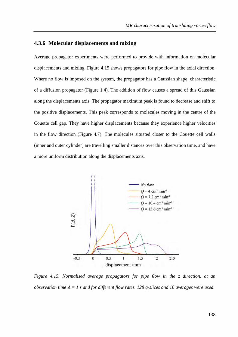
MR characterisation of translating vortex flow

138

4.3.6 Molecular displacements and mixing

Average propagator experiments were performed to provide with information on molecular

displacements and mixing. Figure 4.15 shows propagators for pipe flow in the axial direction.

Where no flow is imposed on the system, the propagator has a Gaussian shape, characteristic

of a diffusion propagator (Figure 1.4). The addition of flow causes a spread of this Gaussian

along the displacements axis. The propagator maximum peak is found to decrease and shift to

the positive displacements. This peak corresponds to molecules moving in the centre of the

Couette cell gap. They have higher displacements because they experience higher velocities

in the flow direction (Figure 4.7). The molecules situated closer to the Couette cell walls

(inner and outer cylinder) are travelling smaller distances over this observation time, and have

a more uniform distribution along the displacements axis.

Figure 4.15. Normalised average propagators for pipe flow in the z direction, at an

observation time Δ = 1 s and for different flow rates. 128 q-slices and 16 averages were used.

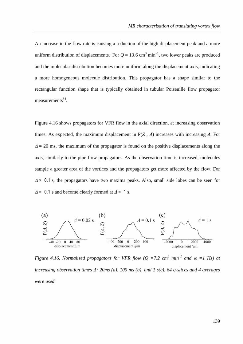
MR characterisation of translating vortex flow

139

An increase in the flow rate is causing a reduction of the high displacement peak and a more

uniform distribution of displacements. For Q = 13.6 cm3 min−1, two lower peaks are produced

and the molecular distribution becomes more uniform along the displacement axis, indicating

a more homogeneous molecule distribution. This propagator has a shape similar to the

rectangular function shape that is typically obtained in tubular Poiseuille flow propagator

measurements34.

Figure 4.16 shows propagators for VFR flow in the axial direction, at increasing observation

times. As expected, the maximum displacement in P(Z , Δ) increases with increasing Δ. For

Δ = 20 ms, the maximum of the propagator is found on the positive displacements along the

axis, similarly to the pipe flow propagators. As the observation time is increased, molecules

sample a greater area of the vortices and the propagators get more affected by the flow. For

Δ > 0.1 s, the propagators have two maxima peaks. Also, small side lobes can be seen for

Δ = 0.1 s and become clearly formed at Δ = 1 s.

Figure 4.16. Normalised propagators for VFR flow (Q =7.2 cm3 min−1 and ω =1 Hz) at

increasing observation times Δ: 20ms (a), 100 ms (b), and 1 s(c). 64 q-slices and 4 averages

were used.

MR characterisation of translating vortex flow

140

Comparison with propagators of pipe flow and TVF can give a better understanding of the

features observed on the VFR propagators. Figure 4.17 displays propagators for pipe flow,

TVF and VFR flow. Propagators of TVF flow were analysed previously (cf. 3.3.3). The

combination of pipe flow and TVF is clearly reflected on the VFR flow propagator. The left

hand-peak of the VFR propagator and its overall broadening shape are characteristic of

molecular circulation within vortices and are clearly resulting from the vortical movement as

the same peak and shape is found for the TVF propagator. However, the VFR propagator is

not symmetric, and the right hand-side part, corresponding to displacements in the direction

of the flow is spreading over a longer distance along the axis.

Figure 4.17. Normalised average propagators for displacements in the z direction at Q =7.2

cm3 min−1 (pipe flow), ω =1 Hz (TVF) and Q =7.2 cm3 min−1 - ω =1 Hz (VFR flow). The

observation time Δ was of 1 s. 64 q-slices and 4 averages were used.

The pronounced peak that persists at zero displacement for both TVF and VFR propagators is

not found on the pipe flow propagator. This peak reveals the presence of low axial

displacement regions in the vortical flows. Such regions could be generated by the strong

MR characterisation of translating vortex flow

141

secondary flow in the radial and azimuthal directions, constraining the molecular

displacement in the axial direction. This is in agreement with previous studies showing that

low molecular displacement regions (or “sticking regions”) can be found in both vortical35

and time-dependant36 flows.

The influence of pipe flow on the VFR flow displacements is to be found on the right-hand

maximum of the VFR propagator (at ∼ 1.1 mm), situated almost at the same position as the

pipe flow maximum (at ∼ 1 mm). The fact that the VFR maximum is slightly advanced is

probably due to axial flow enhancement by the vortical movement in the flow direction. As

the position of the pipe flow propagator maximum depends on Uax, the position of the VFR

propagator maximum could be a function of Uax and UTV. The deviation between the two

peaks could be related to the velocity drift and the VFR maximum position advance explained

by the fact Vd > 1 (the vortex translation velocity is higher than the average flow velocity).

These results show that VFR propagators provide with a unique insight into the molecular

displacement properties within this complex flow. Studies of the effect of flow and rotation

rate on the VFR propagators were performed in order to obtain information on the short time-

scale mixing properties of the VFR.

4.3.7 Flow and rotation rate effect on molecular displacements

Figure 4.18 shows propagators for increasing flow rates at a constant rotation rate (ω = 1 Hz).

Previously (cf. 4.3.5), the right-hand maximum on the VFR propagator was related to the pipe

flow. Comparison with pipe flow propagators at the same flow rates (Figure 4.15), shows that

MR characterisation of translating vortex flow

142

this maximum is always situated at a similar position as the pipe flow propagator maximum.

Also, similarly to the pipe flow propagator observations, this maximum is decreasing with a

flow rate increase. On the other hand, pipe flow does not have any effect on the peak at zero

displacement, showing that both its position and intensity depend on the vortical flow. An

increase in flow rate is to be related with a shift of the left-hand side of the propagator

towards the positive displacements. Except for Q = 10.4 cm3 min−1, this width reduction is

followed by an increase in intensity giving the impression that molecules are “pushed”

towards the positive displacements.

Figure 4.18. Normalised propagators for axial displacements in VFR flow at ω = 1 Hz for

different flow rates. The observation time Δ was of 1 s. 128 q-slices and 16 averages were

used.

The shape of the propagator at low flow rates is more similar to the TVF propagator shape,

showing that higher flow rates tend to reduce the vortical flow. The overall width of the

propagators is reduced at higher flow rates, suggesting a possible reduction in axial dispersion

MR characterisation of translating vortex flow

143

with axial flow rate increase. The analysis of these results shows that the translating tank

model for the VFR flow is not able to address the complexity of the observed phenomena,

while a simple superposition approach as the one suggested by Wereley et al.12 provides with

means for analysing these propagators.

Figure 4.19 shows VFR flow propagators for increasing rotation rates at a constant flow rate

(Q = 7.2 cm3 min−1), in comparison with TVF propagators at the same rotation rates.

Figure 4.19. Normalised propagators for VFR flow (red) at Q = 7.2 cm3 min−1 and in TVF

flow (black) for different rotation rates ω: (a) 1 Hz, (b) 1.5 Hz, (c) 2 Hz and (d) 2.5 Hz. Δ was

of 1 s. 128 q-slices and 16 averages were used. The area between doted lines indicates the

wavelength of the vortex pair including a shift corresponding to the translation of the vortices

during Δ.

MR characterisation of translating vortex flow

144

Again, the centre peak height does not seem influenced by the flow rate at any rotation rate in

this range. As expected, for higher rotation rates the flow effect is less important and the

shape of the VFR propagator is more similar to the TVF one. An increase in rotation rate is

followed by an increase of the propagator width in the negative displacements. For ω = 2.5

Hz (Figure 4.18d) the negative displacements are higher than for the TVF propagator at the

same rotation rate. This might be due to the fact that the flow rate increases displacements in

the high-circulation outer zone of the vortices. This phenomenon at higher rotation rates

seems to support the model11 where the vortical flow is transforming the pipe flow into a

slalom by-pass winding around the vortices. The rotation rate increase is also causing a slight

shift in the position of the flow related right hand side peak. For higher rotation rates, this

peak is found at lower displacements along the axis. This is related to a rotation rate increase

reducing the travelling speed of the vortices (Figure 4.6). For ω = 2.5 Hz, no right-hand

maximum can be seen. This suggests a more homogeneous mixing at these regimes as the

presence of the peak at low rotation rates is causing a more heterogeneous distribution of

molecular displacements along the axis. In fact, the velocities within the vortices have been

shown to increase linearly with rotation rate (cf. chapter 3) while the maximal displacements

on the propagators do not follow the same trend. For an increase of rotation from ω = 1 Hz to

ω = 2 Hz, the increase in the maximal displacements is of 60% (going from 3 mm to 4.8 mm).

At ω = 2.5 Hz the maximal displacements are the same as for ω = 2 Hz while the velocities

are 25% higher. Enhanced molecular displacements seem to be constrained within the vortical

structure at higher rotation rates, suggesting that better intra-vortex mixing is occurring. Due

to the vortical translation, inter-vortex mixing is more difficult to study using these

propagators, but the overall width of the propagators for ω ≥ 2 Hz is found to be equal to the

MR characterisation of translating vortex flow

145

wavelength of the vortex pairs measured at the same regime, suggesting limited mixing

between vortices.

Propagators at higher flow rates can give a better visualisation of this homogenising effect of

rotation. Figure 4.20 shows propagators at Q = 13.6 cm3 min−1 for ω = 1 Hz and ω = 2.5 Hz.

At ω = 1 Hz, the molecular distribution is very heterogeneous, with two peaks in the positive

displacements and a small percentage of molecules travelling over long distances, while the

majority of them is restricted to small displacements At the higher rotation rates the

distribution within the vortex pair is more homogeneous and the molecular displacements are

confined within the distance corresponding to a vortex pair.

Figure 4.20. Normalised propagators for displacements in the z direction for VFR flow at Q

=13.6 cm3 min−1 for ω =1 Hz (red) and ω =2.5 Hz. Δ was of 1 s. 128 q-slices and 16

averages where used for these experiments. The area between doted lines indicates the

wavelength of the vortex pair including a shift corresponding to the translation of the vortices

during the observation time.

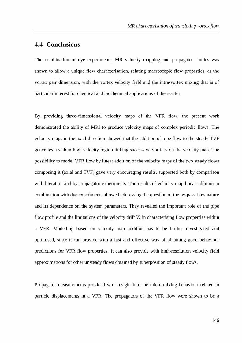
MR characterisation of translating vortex flow

146

4.4 Conclusions

The combination of dye experiments, MR velocity mapping and propagator studies was

shown to allow a unique flow characterisation, relating macroscopic flow properties, as the

vortex pair dimension, with the vortex velocity field and the intra-vortex mixing that is of

particular interest for chemical and biochemical applications of the reactor.

By providing three-dimensional velocity maps of the VFR flow, the present work

demonstrated the ability of MRI to produce velocity maps of complex periodic flows. The

velocity maps in the axial direction showed that the addition of pipe flow to the steady TVF

generates a slalom high velocity region linking successive vortices on the velocity map. The

possibility to model VFR flow by linear addition of the velocity maps of the two steady flows

composing it (axial and TVF) gave very encouraging results, supported both by comparison

with literature and by propagator experiments. The results of velocity map linear addition in

combination with dye experiments allowed addressing the question of the by-pass flow nature

and its dependence on the system parameters. They revealed the important role of the pipe

flow profile and the limitations of the velocity drift Vd in characterising flow properties within

a VFR. Modelling based on velocity map addition has to be further investigated and

optimised, since it can provide with a fast and effective way of obtaining good behaviour

predictions for VFR flow properties. It can also provide with high-resolution velocity field

approximations for other unsteady flows obtained by superposition of steady flows.

Propagator measurements provided with insight into the micro-mixing behaviour related to

particle displacements in a VFR. The propagators of the VFR flow were shown to be a

MR characterisation of translating vortex flow

147

combination of the pipe flow and TVF propagators, revealing the limitations of the simplistic

translating tank model for the VFR flow. The effects of flow and rotation on the micro-

mixing properties of the VFR were studied using propagator analysis. At low rotations, high

flows were shown to generate a heterogeneous distribution of molecular displacements along

the reactors length, while an increase in rotation was linked with better intra-vortex mixing.

(1) Judat, B.; Racina, A.; Kind, M. Chem. Eng. Technol. 2004, 27, 287.

(2) Forney, L. J.; Pierson, J. A. AIChE J. 2003, 49, 727.

(3) Wolinski, J.; Wronski, S. Chem. Eng. and Process. 2009, 48, 1061.

(4) Haut, B.; Ben Amor, H.; Coulon, L.; Jacquet, A.; Halloin, V. Chem. Eng. Sci.

2003, 58, 777.

(5) Resende, M. M.; Sousa, R.; Tardioli, P. W.; Giordano, R. L. C.; Giordano, R.

C. AIChE J. 2005, 51, 314.

(6) Kataoka, K.; Hongo, T.; Futagawa, M. J. Chem. Eng. Jpn 1974, 8, 4.

(7) Giordano, R. C.; Giordano, R. L. C.; Prazeres, D. M. F.; Cooney, C. L. Chem.

Eng. Sci. 1998, 53, 3635.

(8) Legrand, J.; Coeuret, F. Chem. Eng. Sci. 1986, 41, 47.

(9) Cohen, S.; Marom, D. M. Chem. Eng. J. and Biochem. Eng. 1983, 27, 87.

(10) Lueptow, R. M.; Docter, A.; Min, K. Y. Phys. Fluids a-Fluid 1992, 4, 2446.

(11) Haim, D.; Pismen, L. M. Chem. Eng. Sci. 1994, 49, 1119.

(12) Wereley, S. T.; Lueptow, R. M. Phys. Fluids 1999, 11, 3637.

(13) Desmet, G.; Verelst, H.; Baron, G. V. Chem. Eng. Sci. 1996, 51, 1287.

(14) Desmet, G.; Verelst, H.; Baron, G. V. Chem. Eng. Sci. 1996, 51, 1299.

MR characterisation of translating vortex flow

148

(15) Giordano, R. L. C.; Giordano, R. C.; Prazeres, D. M. F.; Cooney, C. L. Chem.

Eng. Sci. 2000, 55, 3611.

(16) Syed, A.; Fruh, W. G. J. Chem. Technol. Biot. 2003, 78, 227.

(17) Elkins, C. J.; Alley, M. T. Exp. Fluids 2007, 43, 823.

(18) Henkelman, R. M.; Bronskill, M. J. Med. Phys. 1987, 14, 506.

(19) Uludag, Y.; Powell, R. L.; McCarthy, M. J. AIChE J. 2004, 50, 1662.

(20) Moser, K. W.; Raguin, L. G.; Harris, A.; Morris, H. D.; Georgiadis, J.;

Shannon, M.; Philpott, M. Magn. Reson. Imaging 2000, 18, 199.

(21) Han, S. I.; Stapf, S.; Blumich, B. Phys. Rev. Lett. 2001, 8714.

(22) Vallatos, A.; Wilson, M. C. T.; Taylor, A. F.; Britton, M. M. Europhys. Lett.

2012.

(23) Sczechowski, J. G.; Koval, C. A.; Noble, R. D. Chem. Eng. Sci. 1995, 50,

3163.

(24) Campero, R. J.; Vigil, R. D. Chem. Eng. Sci. 1997, 52, 3303.

(25) Resende, M. M.; Tardioli, P. W.; Fernandez, V. M.; Ferreira, A. L. O.;

Giordano, R. L. C.; Giordano, R. C. Chem. Eng. Sci. 2001, 56, 755.

(26) Raguin, L. G.; Georgiadis, J. G. J. Fluid Mech. 2004, 516, 125.

(27) Resende, M. M.; Vieira, P. G.; Sousa, R.; Giordano, R. L. C.; Giordano, R. C.

Braz. J. Chem. Eng. 2004, 21, 175.

(28) Richter, O.; Hoffmann, H.; Kraushaar-Czarnetzki, B. Chem. Eng. Sci. 2008,

63, 3504.

(29) Richter, O.; Menges, M.; Kraushaar-Czarnetzki, B. Chem. Eng. Sci. 2009, 64,

2384.

(30) Coles, D. J. Fluid Mech. 1965, 21.

MR characterisation of translating vortex flow

149

(31) Seymour, J. D.; Callaghan, P. T. AIChE J. 1997, 43, 2096.

(32) Bird, R. B.; Stewart, W. E.; Lightfoot, E. N. Transport phenomena, 2nd, Wiley

international ed.; J. Wiley: New York, 2002.

(33) Howes, T.; Rudman, M. AIChE J. 1998, 44, 255.

(34) Callaghan, P. T.; Xia, Y. J. Magn. Res. 1991, 91, 326.

(35) Young, W.; Pumir, A.; Pomeau, Y. Phys. Fluids a-Fluid 1989, 1, 462.

(36) Meiss, J. D.; Ott, E. Phys. Rev. Lett. 1985, 55, 2741.

Molecular displacement simulations using MR data

150

5 Molecular displacement simulations using MR data

5.1 Introduction

Theoretical studies of axial dispersion in TVF and VFR flow1 have been made using models

that lead to transport equations including a dispersion tensor2. These studies provided with

good estimates of axial dispersion for stationary vortex flow (TVF) but not for translating

vortex flow (VFR). Most theoretical studies of flow patterns in Couette cells focus on the

Eulerian properties of the flow, and present limitations in addressing micro-mixing properties

that necessitate a Lagrangian analysis3. Similarly, the results presented in the previous

chapters show that MR velocity and diffusion/dispersion mapping cannot give quantitative

information on molecular displacements and that this information could be assessed by

propagator measurements. In particular, knowing the molecular displacements in a VFR could

allow characterisation of the axial dispersion while providing quantitative information on

plug-flow properties, by probing the extent of inter-vortex mixing. In the context of chemical

engineering, information on molecular displacements and mixing is often more crucial in

characterising the properties of a reactor than the velocity field. For example, when flow is

coupled with autocatalysis, quantitative information on molecular displacements can provide

a means to evaluate the relative input of transport and reaction into the propagation of

autocatalytic waves and fronts 4,5.

However, propagator measurements are constrained to short observation times (Δ ≤ 1 s), due

to MR relaxation. Previous studies6 have addressed this limitation by producing simulated

propagators for longer times using molecular displacement models. Similar models, based on

Molecular displacement simulations using MR data

151

fluid particle tracking, were also used for studying mixing and dispersion in wavy TVF3,7. In

such particle-tracking simulations the velocity field is calculated using the NS equation. In the

case of complex vortical flows, velocity field simplifications are required, limiting the

quantitative nature of the results. The present work overcomes this limitation by using

experimental MR velocity and diffusion/dispersion maps. Velocity distribution histograms

have been shown to reproduce the molecular distribution features in propagator

measurements8,9. Here, molecular displacements are simulated using the pixel average

velocity and diffusion/dispersion coefficient provided by experimental maps. Considering the

symmetry of the studied flows in the azimuthal direction, two-dimensional simulations were

performed, where two-dimensional coordinates identified each molecule’s position. By using

a sufficiently large number of molecules in the simulation, the percentage distribution of

displacements along an axis can be plotted as a propagator along this axis.

Initially, simulations for short observation times were performed (Δ ≤ 1s). The obtained

simulated propagators for pipe flow, TVF and VFR flow were compared with experimental

propagators presented in the previous chapter. This comparison allowed the verification of the

method. Following this, simulations for observation times that are not accessible

experimentally were performed. These simulations enable molecular transport and mixing to

be assessed over longer-time scales, allowing plug-flow, by-pass flow and inter-vortex mixing

to be quantified10. Also, since two-dimensional coordinates identify the molecular trajectories,

the simulations allow for molecular pathways on the map surface to be predicted. These

results provide with quantitative and qualitative spatially resolved information on the mixing

properties within each flow.

Molecular displacement simulations using MR data

152

Propagator simulations can show the transport of molecules. Molecular trajectories can also

be observed experimentally using a chemical front. Where an autocatalytic reaction is used, it

is possible to detect the transport of even small numbers of molecules. The simulation results

are compared with experimental studies of chemical front propagation in TVF and VFR flow.

Chemical waves are obtained using the bromate-sulfite pH clock reaction11. The reaction is

followed by a sharp drop in pH that is used to visualise the propagation of chemical fronts12.

These fronts have been shown to be sensitive to convection effects and can be particularly

useful in the study of transport processes within flow systems. This study shows how

molecular displacement simulations based on experimental MR data allow to understand and

predict the shape of chemical fronts propagating through stationary and translating vortical

flow. The VFR simulations allow prediction of the effects of small numbers of molecules

travelling faster (by-pass flow) or slower (drag flow) than the translating vortices.

5.2 Experimental

5.2.1 Molecular displacement simulations

Simulations were performed using Matlab on a PC. The velocity and diffusion/dispersion

fields were created using experimental velocity (Uy, Uz) and diffusion/dispersion (Dy, Dz)

maps for axial flow at Q = 7.2 cm3 min−1, Taylor vortex flow at ω = 1 Hz and VFR flow at Q

= 7.2 cm3 min−1and ω =1 Hz. A more detailed analysis of the properties of these flows is

provided in chapters 3 and 4. Molecular displacements in the azimuthal direction were

assumed to be symmetric. Also the flow fields present symmetry with respect to the inner

cylinder. This allowed considering only the velocity and diffusion/dispersion fields obtained

Molecular displacement simulations using MR data

153

on one side of the Couette cell gap.

As discussed earlier, diffusion/dispersion maps do not provide with quantitative values of

diffusion and dispersion within each voxel (cf. 3.3.1.2). This is due to the fact that the

measured values are affected by both velocity shear and the pixel size. An alternative to the

use of these maps would have been to use a constant self-diffusion coefficient for these

simulations. But for sufficiently long mixing times, the effect of diffusion-dispersion on

overall molecular displacements was expected to be negligible compared to the effect of the

velocity field. In fact, for all the simulations with mixing times Δ > 100 ms presented in this

chapter, replacing the diffusion/dispersion maps with a constant diffusion coefficient gave

similar molecular distribution results. Hence, the errors coming from the use of the

experimental diffusion/dispersion maps were only expected to play a role for short simulation

times. Moreover, using these maps allowed accounting for effects related to spatial

inhomogeneity of dispersion.

The simulations used n molecules identified by their two-dimensional coordinates in the

velocity field plan. For simulations of stationary and translating vortices, the molecules were

evenly distributed throughout several vortex pairs within the velocity maps. The same

distribution was used in axial flow simulations. The dimensions of the experimental velocity

and diffusion/dispersion maps do not allow simulating displacements over more than a

distance corresponding to five vortex pairs. For pipe flow, where velocity is constant along

the axial direction, an average velocity profile was considered over longer distances. For the

vortical flows, spatial periodicity allowed for longer velocity maps to be constructed by

juxtaposition of series of an experimental map region corresponding to one vortex pair. For

Molecular displacement simulations using MR data

154

the VFR flow, as experimental diffusion/dispersion maps were not available, an estimation of

the dispersion field was made. Regions of high and low dispersion could be identified from

the diffusive attenuation produced by the PGSE velocity imaging experiments13. The

estimated diffusion/dispersion maps were then obtained by scaling the diffusive attenuation

field to the TVF diffusion/dispersion map. Also, an additional modification was required in

order to take the observed translation of the vortices into account, which allowed the velocity

and diffusion/dispersion fields to translate at a velocity UTV.

Time steps, dt, were considered for these simulations. The total number of steps, N, was given

by N = Δ / dt, where Δ is the observation time to be simulated. At every time step, dt, the

displacement of each molecule ni of coordinates (yi,zi) was defined by a velocity and a

diffusion/dispersion step. The velocity step was determined using the experimental velocity

maps Uy and Uz. For the diffusive step, the direction was determined by a randomly generated

angle θ and the magnitude was calculated using the diffusion/dispersion maps Dy and Dz.

Displacements due to velocity and diffusion in each direction where then added to the initial

coordinates to define the final coordinates yi(t+dt) and zi(t+dt).

A bounce-back boundary condition was employed for molecules near the reactor walls. If the

distance to the wall was found to be smaller than the distance ddt to be traveled during dt, the

molecule was simply considered to travel until the wall and perform the rest of ddt in the

reverse direction. A minimum of three repetitions for each set of parameters was performed.

The Maltab code used for these simulations is included in Appendix B.

After N × dt steps, the overall displacement for each molecule ni along the z-axis was

determined by comparing the zi coordinates of the initial and final positions. The displacement

Molecular displacement simulations using MR data

155

axis was separated in bins and the number of molecules to attain each bin at the end of the

simulation was counted. Simulated normalised propagators for a given observation time Δ

were obtained by plotting the proportion of molecules at each displacement bin against

displacements.

Molecular paths were tracked either by calculations of molecular density per pixel at different

observation times, either by calculation of the residence time of molecules per pixel. In this

second approach, a matrix counting how many molecules attend each pixel during the

simulation was produced to give information on molecular displacements over time. A 2D

plot of theses matrices shows high and low circulation pathways within the flow. Because the

attendance in some pixels was orders of magnitude higher than in others, a logarithmic scale

was used to reveal minor paths taken by molecules.

500 000 molecules were used for all the simulations. The observation times Δ were of 20 ms,

100 ms, 1 s and 1 min. For simulations with Δ < 1 s, dt was of 0.1 ms and 40 bins were used

for the displacement axis. For simulations with Δ ≥ 1 s, dt was of 1 ms and 60 bins were used

for the displacement axis. For the VFR simulations the velocity and diffusion/dispersion

fields were translating at a velocity UTV = 0.81 mm s−1, in accordance with experimental

results obtained in chapter 4.

5.2.2 Chemical front propagation in vortical flow

A bromate-sulfite reaction mixture was obtained by mixing two separate reagent solutions.

Solution A contained sodium bromate (0.1 M), while solution B contained sodium sulfite

Molecular displacement simulations using MR data

156

(0.26 M) and a colour pH-indicator (0.5 g in 1L) both in deionised water. Two pH-indicators

were used for obtaining contrast between the reactants and the more acidic products:

bromocresol purple (yellow product front in purple reactant solution) and methyl red (red

product front in orange reactant solution). The solutions were mixed and then pumped into the

Couette cell. The waves were initiated using a 0.5 mL injection of 1 M sulphuric acid at the

inlet of the reactor. The Couette cell used for these experiments is described in previous

sections (cf. 3.2.1 and 4.2.1). The viscosity ν of the solutions was on the order of 1 mm2 s−1 at

22 ± 0.5 ˚C, similar to the viscosity of the solutions used for the velocity and

diffusion/dispersion imaging experiments (Chapters 3 and 4). A rotation rate of ω = 1 Hz and

a flow rate Q = 7.2 cm3 min−1 were used for these experiments. Each experiment was

repeated a minimum of three times. Optical images of the reactor were acquired every 5 s.

The optical imaging technique is described in previous sections (cf. 4.2.3).

Molecular displacement simulations using MR data

157

5.3 Results and discussion

5.3.1 Molecular displacements and propagator simulations

Figure 5.1 shows experimental (a - c) and simulated (d - f) propagators for pipe flow at the

same observation times Δ. Simulated propagators are shown to reproduce the main features of

the experimental ones (positive displacements and formation of a maximum). Also, both the

position of the maximum peak and the overall displacements are found to be in quantitative

agreement.

Figure 5.1. (a)–(c) Experimental propagators and (d)–(f) simulated propagators at

increasing observation times, for pipe flow at Q=7.2 cm3 min−1.

Figure 5.2 shows experimental (a - c) and simulated (d - f) propagators for TVF flow at the

same observation times Δ. At low observation times (Δ ≤ 100 ms), the simulated propagators

have less clear structural features than the experimental ones, but for Δ = 1 s all the features of

Molecular displacement simulations using MR data

158

the measured propagator can be identified (centre maximum and side lobes). Again

quantitative agreement is found both for the overall displacements and the position of the

main features.

Figure 5.2. (a)–(c) Experimental propagators and (d)–(f) simulated propagators at

increasing observation times, for Taylor vortex flow at ω =1 Hz.

Figure 5.3 shows experimental (a - c) and simulated (d - f) propagators for VFR flow at the

same observation times Δ. Although the agreement is not as good as for pipe fow or TVF, the

simulation reproduces all the structural features of measured molecular displacements in the

VFR. Discrepancies in the overall broadening of the VFR propagators may be related with the

use of an estimated diffusion/dispersion map for the simulated ones. The main difference

arises from a shift in position of the maximum associated with the pipe flow (right-hand

maximum on the propagators). There seems to be a delay for the formation and the overall

displacement of this maximum in the case of the simulation. In the experimental propagator,

Molecular displacement simulations using MR data

159

this maximum is always found at higher displacement compared to the pipe flow maximum,

while for the simulated propagators it is found at a lower displacement.

Figure 5.3. (a)–(c) Experimental propagators and (d)–(f) simulated propagators at

increasing observation times, for VFR flow at ω = 1 Hz and Q = 7.2 cm3 min−1.

This difference could be attributed to dispersion enhancement between vortex pairs, which is

not taken into account in our model. In fact, the translational movement of the vortex pairs

could give rise to Taylor dispersion14 as measurements in TVF and VFR show that the

addition of pipe flow is followed by an increase in axial dispersion15. In their theoretical study

on axial dispersion within VFR flow, Howes and Rudman1 suggested that discrepancies

between their results and experimental data could be explained by the existence of a further

mechanism for axial dispersion caused by the difference in velocity between the vortex

translation and the average axial velocity (UTV – Uax). Comparison between simulated and

Molecular displacement simulations using MR data

160

experimental propagator data could provide with information on dispersion linked with such

molecular displacements.

As it has also been observed in TVF, the structural features of experimental propagators (two

peaks, middle and side lobes) become clear in the simulated propagators for VFR flow as the

observation time increases. At higher Δ, coherent molecular displacements such as the ones

imposed by the velocity maps, play a dominant role in determining the overall molecular

displacements. Therefore, it is expected that discrepancies related to diffusion/dispersion are

reduced, and simulated propagators tend to be in better agreement with experimental ones. To

confirm the secondary role of dispersion, longer time-scale simulations were performed on

pipe flow and TVF. These simulations showed that diffusion/dispersion map effects on the

overall molecular distribution are minimal at high observation times (Δ). Thus, even though

the VFR simulated propagators do not completely capture the displacement characteristics of

flow in the VFR for low observation times, they do allow us to probe molecule trajectories

and explore displacements in excess of what can be measured experimentally, where Δ is

typically limited to ≤ 1s.

5.3.2 Long time scale displacements and axial dispersion

Figure 5.4 shows simulated propagators for pipe and VFR flows at an observation time of Δ =

1 min. As expected, pipe flow spreads the molecules along the axial direction with a

maximum close to the higher displacements (at 60 mm). In the case of the VFR propagator

simulation, the molecular spread along the axial direction is reduced both on high and low

displacements. Hence, at the same flow rate the vortical flow is shown to reduce axial

Molecular displacement simulations using MR data

161

dispersion. This reduction of molecular spread reflects the plug-flow properties of the

translating vortices.

Figure 5.4. Simulated propagators at Δ = 1 min, for pipe flow (black line) at Q =7.2 cm3

min−1 and VFR flow (red line) at ω =1 Hz and Q = 7.2 cm3 min−1, with dye injection

photograph inlay.

The simulated propagators can provide with quantitative information of the mixing properties

within the VFR. Over the time of the simulation, vortices translate up to 49 mm

(approximately the length of 6 vortex pairs). What this propagator reveals is partial plug-flow,

with 95% of molecular displacements limited to three vortex pairs.

A surprising feature of the VFR propagator is the presence of peaks and troughs. The distance

between the peaks corresponds to approximately one vortex pair wavelength, λ. At the end of

the simulation, each vortex pair on the velocity map was situated between a peak and a trough

on the propagator, indicating that higher molecular concentration is expected in one over two

Molecular displacement simulations using MR data

162

vortices. These results are in agreement with the dye experiment results (cf. 4.3.1) where

heterogeneous distribution of molecules into successive vortices was suggested. (Figure 5.4).

These simulations allow, for the first time, to predict residence times and quantify inter-vortex

mixing and plug-flow. In the case of the Δ = 1 min simulation, 72 ± 10 % of the molecules

remained in the vortex pair in which they started, while 26 ± 10 % mixed with the vortices

behind and 2 ± 1 % mixed with the vortices ahead. This indicates that the plug-flow

properties of the reactor are more affected by molecules moving slower than the vortices

(drag) than by ones moving faster (by-pass). This was expected, as the vortices move faster

than the average axial velocity (Vd > 1), and was also suggested by the dye experiments,

where the dye front was sharp while the back was spreading over several vortex-pairs. To get

a better insight into the mechanisms that underlie the molecular distribution within these

flows spatial information is required in order to identify molecular pathways and regions of

high and low mixing.

5.3.3 Molecular paths in pipe flow

Molecular paths in the pipe flow simulation for molecules starting from a region

corresponding to two vortex pairs are shown in Figure 5.5a. At t ≥ 10 s, the shape of the

molecular pathways reflects the typical parabolic shape of Poiseuille flow velocity profiles.

The longer displacements are found in the middle of the gap, in the region of the velocity

maxima. Similarly to the velocity profile for pipe flow (Figure 4.7), the maximum is situated

slightly towards the inner cylinder. This effect can be noticed more clearly at higher

observation times where the molecules are found at higher displacements on the inner

Molecular displacement simulations using MR data

163

cylinder part, causing a dissymmetry of the parabolic shape. While the friction at the walls

causes a dispersion of the molecules depopulating the sides, the middle part of the front stays

densely populated during the simulation. This explains the presence of the peak at high

displacements observed in the pipe flow propagators (Figure 5.1c and Figure 5.4). The use of

a logarithmic scale (Figure 5.5b) reveals less populated areas of the map. In the case of

vortical flows, where the spread of the molecules is expected to be greater, a logarithmic scale

can allow identifying low-density molecular paths.

Figure 5.5. (a) Maps showing the molecular density per pixel in a simulation of molecular

displacements in pipe flow at different observation times. (b) Map at t = 60 s plotted on a

log10 scale.

Molecular displacement simulations using MR data

164

5.3.4 Molecular paths in TVF

The velocity maps used for the simulation of molecular displacements in TVF at ω = 1 Hz are

shown in Figure 5.6a. These maps were obtained by juxtaposing a region of the experimental

velocity maps corresponding to one vortex pair. The region of the maps corresponding to the

initial molecule distribution covers four vortex pairs. Molecular paths for molecules starting

from this region are shown in Figure 5.6b for observation times of 30 s and 60 s.

Figure 5.6. (a) Velocity maps of TVF flow at ω =1 Hz. (b-c) Maps showing the residence time

(tres) per pixel, over 30 s and 60 s, for molecules starting from the region indicated in part (a).

The maps are plotted on linear (b) and log10 (c) scale.

Molecular displacement simulations using MR data

165

Contrary to the pipe flow simulations, molecular spread was very important during the TVF

simulations, making it difficult to identify the paths followed by the molecules on molecular

density maps. To address this issue, pixel intensity in these maps corresponds to the number

of times molecules were found in each pixel during the simulation, or molecular residence

time (tres). Figure 5.6b shows the presence of high-movement square pathways on the outer

region of the vortices. Molecules seem trapped in these pathways as very low movements are

seen in the vortex core region. Molecular displacement in these high-movement regions can

help explaining the features of the TVF propagators (Figure 5.2). Molecules moving in the

axial direction (z) correspond to the high displacement side lobes seen in TVF propagators.

Molecules moving in the radial direction can probably explain the maxima of the TVF

propagator at zero displacement: despite the fact that these molecules make big displacements

along the radial direction, they are not moving along the axial direction. In these secondary

flow areas in the radial direction, the paths are larger when the flow is coming towards the

inner cylinder and narrower when it is leaving it.

As discussed, the use of a logarithmic scale for the molecular path map allows probing lower

circulation paths. Figure 5.6c reveals that enhanced displacements are performed by a

relatively small number of molecules that travel in the outer region. These paths seem to go

further in one direction (lower part of the image). This might be due either to gravity effects

reflected in the velocity and diffusion/dispersion maps, either to small errors in the

reconstruction of the long maps by addition of successive bits of the experimental maps. In

the latter case, an overlapping of the velocity maps of the order of a pixel size might favour

one direction rather than the other. These displacements may be seemingly negligible,

however they may play an important role in transmitting a chemical signal thus helping to

Molecular displacement simulations using MR data

166

explain features of chemical front propagation through these systems. This is particularly the

case when the flow is coupled with autocatalytic chemistry, where only a small amount of

autocatalyst is required to carry the chemical wave16.

5.3.5 Molecular paths in VFR flow

The z-direction velocity map used for the simulation of molecular displacements in VFR flow

at ω = 1 Hz and Q = 7.2 cm3 min−1 is shown in Figure 5.7a. Similarly to TVF, this map was

obtained by juxtaposition of a region of the experimental velocity maps corresponding to one

vortex pair. The molecules were seeded uniformly in a region corresponding to a single

vortex pair highlighted by the doted rectangle.

Molecular path simulations in VFR flow for an observation time of 60 s are shown in Figure

5.7b. These paths correspond to molecular displacements in translating vortices from the

point of view of a stationary observer. As the vortices are translating by a distance

corresponding to 6 vortex pairs during this observation time, the vortical structure is not

reflected in these paths as for the TVF flow. The highest circulation regions are observed on

the walls of the reactor (red colour) and correspond to the flow generated in the outer region

of the vortices. More circulation (higher intensity) is found in the outer cylinder region than

the inner cylinder one. The middle of the reactor is less densely populated, probably due to

the lower circulation in the vortex core regions.

Molecular displacement simulations using MR data

167

Figure 5.7. Velocity map of VFR flow at ω =1 Hz and Q = 7.2 cm3 min−1 (the arrow shows the

direction of the travelling vortices) and map showing the residence time (tres) per pixel, over Δ

= 60 s, for molecules starting from the single vortex pair highlighted in the doted rectangle.

The residence times are plotted on a log10 scale.

Contrary to TVF simulation results (Figure 5.6), circulation in the centre of the VFR gap

(yellow colour) is shown to be homogeneous. The translation of the vortices causes the pixel

attendance along the axial direction to be averaged. An average of the TVF map along the z

direction gives similar results, with the walls being highly populated and the attendance at the

centre of the gap corresponding to an average between the vortex core circulation and the

Molecular displacement simulations using MR data

168

outer region circulation along the radial direction. Close to the initial molecular distribution

region this averaging is not well performed and two high circulation paths going from one

wall to the other can be seen. In fact, at the initial stages of the simulation, the vortical flow

dominates the molecular pathways since its velocities are three to five times greater than the

vortex translation velocity UTV. This causes the initial paths in the middle of the gap to be

more noticeable.

This simulation provides with poor insight into the mixing properties of the vortical flow. In

this stationary reference frame, molecular paths do not coincide with the velocity streamlines

of the vortices. This explains why velocity field features, as the slalom high velocity regions,

are not reflected on the molecular paths. In order to facilitate the comparison between the

molecular paths and velocity fields both must be on the same reference frame. This can be

obtained by tracking the molecules in the reference frame of the translating vortices. To get a

better understanding of the role of the vortices in the molecular displacements within this

flow and characterise by-pass and drag flow within the system, the same simulations were

performed with molecular displacements tracked on a map translating at the same speed as the

velocity and diffusion/dispersion maps, UTV.

Figure 5.8 shows these molecular displacements in comparison with the velocity maps in the

axial and radial direction. The velocity field features can be identified on the molecular paths.

As the propagator simulations suggest (Figure 5.4), the majority of the molecules remain

within the vortex pair they were initially seeded. The highest molecular attendance in this

map (red colour) is identified at the interface of opposite direction velocities between the

vortex pairs. The circulation paths out of the initial vortex pair correspond to by-pass if they

Molecular displacement simulations using MR data

169

are situated downstream (above the vortex pair), or drag if they are situated upstream (below

the vortex pair).

Figure 5.8. Velocity maps of VFR flow in the axial and radial directions at ω =1 Hz and Q =

7.2 cm3 min−1 and map showing the residence time (tres) per pixel, over Δ = 60s s, for

molecules starting from the single vortex pair highlighted in the doted square. All maps are

translating with a velocity UTV so the molecular paths are shown in the reference frame of the

translating vortices. The residence times are plotted on a log10 scale.

This map shows the importance of drag in this system where the vortices travel faster than the

average axial velocity (Vd > 1). The drag is mainly situated on the outer cylinder side. The

molecules leave the vortex pair attracted by the negative velocities along z in the following

vortex pair. As soon as they enter the following vortex pair, these molecules follow the path

in the high circulation outer vortex zone. Some of them are transported by the secondary flow

Molecular displacement simulations using MR data

170

in the middle of the vortex pair and start wrapping around the vortices. Notice that due to the

fact that the high circulation path brings the molecules in the middle of the vortex pair, the

lower vortex tends to by populated before the upper one. This is probably the cause of the

heterogeneous distribution observed in the simulated propagators (Figure 5.4).

Heterogeneous distribution can also be noticed in the by-pass flow identified at the top of the

image. Long time-scale propagators showed that by-pass molecular paths represent a very

small percentage of molecules. As for drag, the by-pass molecules are leaving from the outer

cylinder side and wrap around the outer region of the preceding vortex. Some of these

molecules seem to reach the vortex core after following the high circulation path in the outer

region that leads them in the inter-vortex area. Those that do not mix with the first vortex

seem to wrap around the second vortex without reaching its inner core, and when arrived at

the outer cylinder wall, they follow the circulation path leading to the following vortex pair.

The percentage of these molecules is small, however, where a chemical system is coupled to

VFR flow, this by-pass flow can play a substantial role in the propagation of chemical waves

and fronts.

5.3.6 Chemical wave propagation in TVF

Figure 5.9 shows bromate-sulfite chemical fronts (in yellow), visualised with bromocressol

purple pH indicator, propagating upwards and downwards through TVF at ω = 1 Hz. The

front shape seems similar for upwards and downwards propagating waves. The chemical

wave propagates through the successive vortices until it consumes the entire Couette cell. It

initially reaches the outer part of the vortices and the inter-vortex areas.

Molecular displacement simulations using MR data

171

Figure 5.9 Upwards (a) and downwards (b) propagating wave front in TVF at ω = 1 Hz.

Each picture was taken at 5 s intervals.

As the yellow front spreads through the outer vortex region, the vortex core can be

distinguished as a region in purple in these images. The chemical front propagation in the

outer regions has an advance of 2-3 vortices compared to its propagation in the core regions.

This is a clear indication of the existence of high-circulation paths in the vortex outer zones.

These results are in agreement with previous studies of chemical front propagation through

TVF vortices5,16,17, probing the high-circulation outer zone. The molecular path simulations

for TVF (Figure 5.6) also reproduced these zones. In the simulations, molecular

displacements in the outer vortex regions were found to have 3-4 vortices of advance. A more

detailed comparison, between the simulations and the experiments could allow identifying the

relative inputs of reaction and transport in the propagation of this wave.

Molecular displacement simulations using MR data

172

5.3.7 Chemical wave propagation in VFR flow

Although chemical reactions are often used to characterise transport properties of the

travelling vortices produced in a VFR18, no published studies of autocatalytic front

propagation in this system has been identified in the literature. Figure 5.10 shows chemical

waves propagating through translating vortices in a VFR (Q = 7.2 cm3 min−1, ω = 1 Hz)

visualised wit bromocressol purple (yellow) and methyl red (red). The chemical waves,

initiated at the inlet of the reactor, propagate in the same direction as the travelling vortices

until reaching the outlet of the reactor. As fresh reactants keep on entering the reactor, after

the wave passes, the solution switches back to its steady state. That means that each wave can

be characterised both by its front and backside.

In Figure 5.10a bromocressol purple is used to visualise the chemical front. The yellow front

is not uniform and the inter-vortex regions are maintained in the purple state much longer

than the vortex core. This reveals the two mixing regions (inner and outer) identified for TVF.

At this regime the vortices travel faster than the axial flow (Vd > 1). Molecular simulations

showed the presence of important drag at this regime, which means that matter is left behind

the travelling vortex pairs. This drag seems to be mostly concentrated in the inter-vortex areas

where the purple colour is located. In fact, as the front is yellow and the drag purple the latter

is easier to characterise with this chemical system.

In Figure 5.10b methyl red is used to visualise the front. Methyl red gave a better contrast for

the front (red front in orange background). Aso, the transition from the reactants to the

products seems less sharp than for the bromocressol purple, allowing different information on

Molecular displacement simulations using MR data

173

mixing to be gained. These images reveal a heterogeneous distribution of the waves into

successive vortices. One vortex of each pair “switches” to red before the other, showing that

non-uniform mixing occurs in the axial direction. The vortices in the red state seem smaller,

probably because the inter-vortex area is in orange state. Note that simulated VFR

propagators showed a similar distribution of molecular displacements into successive vortices

(Figure 5.4).

Figure 5.10. Downstream front of (a) bromocressol purple and (b) methyl red waves in VFR

flow at ω = 1 Hz and Q = 7.2 cm3 min−1. Each picture was taken at 5 s intervals. The arrow

indicates the flow direction.

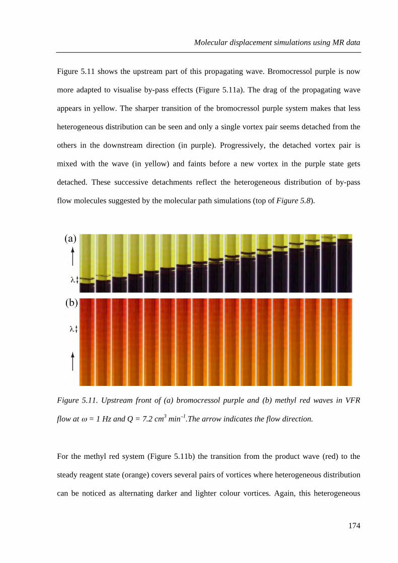
Molecular displacement simulations using MR data

174

Figure 5.11 shows the upstream part of this propagating wave. Bromocressol purple is now

more adapted to visualise by-pass effects (Figure 5.11a). The drag of the propagating wave

appears in yellow. The sharper transition of the bromocressol purple system makes that less

heterogeneous distribution can be seen and only a single vortex pair seems detached from the

others in the downstream direction (in purple). Progressively, the detached vortex pair is

mixed with the wave (in yellow) and faints before a new vortex in the purple state gets

detached. These successive detachments reflect the heterogeneous distribution of by-pass

flow molecules suggested by the molecular path simulations (top of Figure 5.8).

Figure 5.11. Upstream front of (a) bromocressol purple and (b) methyl red waves in VFR

flow at ω = 1 Hz and Q = 7.2 cm3 min−1.The arrow indicates the flow direction.

For the methyl red system (Figure 5.11b) the transition from the product wave (red) to the

steady reagent state (orange) covers several pairs of vortices where heterogeneous distribution

can be noticed as alternating darker and lighter colour vortices. Again, this heterogeneous

Molecular displacement simulations using MR data

175

distribution of molecules seems to be explained by the molecular path simulations, where

drag is found to affect differently one over two vortices of each pair (bottom of Figure 5.8).

This suggests that comparison with propagator simulations over similar observation times can

allow a quantification of this heterogeneous distribution in the axial direction.

5.4 Conclusions

Taking the examples of pipe flow, TVF and VFR flow in a Couette cell, the study presented

in this chapter demonstrates that the combination between magnetic resonance techniques

(MR flow imaging - propagator measurements) and molecular displacement simulations is

able to uniquely characterise mixing properties in complex laminar flows10. Comparison with

experiments of autocatalytic wave propagation showed that molecular pathway simulations

can also provide with a way to analyse the coupling between reaction and transport in

complex flows.

For small observation times these simulations produced propagators in good agreement with

experimental ones. Increasing the simulation observation time allowed obtaining information

on molecular transport over longer time scales. The simulated propagators provided with

quantitative information regarding molecular dispersion, mixing and residence times.

Simulated molecular path maps provided with a deeper insight into the micro-mixing

properties of the flows. They allowed understanding the features of experimental propagators,

linking molecular displacement measurements with mixing properties. In the case of

travelling vortex flow, the simulations enabled a quantitative analysis of drag and by-pass

Molecular displacement simulations using MR data

176

effects, showing how these can co-exist with the plug-like flow properties of the system.

These results can be of particular interest in chemical engineering applications for analysing

the mixing properties of chemical reactors.

Molecular displacement simulations reproduced the main features of autocatalytic bromate-

sulfite waves propagating through vortical flow. Simulated VFR propagators provided insight

into the surprising phenomenon of segmented chemical fronts by showing that heterogeneous

molecular distribution within successive vortices is occurring. Also, statistically insignificant

molecular displacements, that may not compromise the plug-like flow properties of the

reactor, were shown to play crucial role in the chemical wave propagation and shape.

Comparison between simulations and systems where autocatalytic chemistry is coupled with

vortical flow could allow a quantitative analysis of how flow and chemistry affect the

propagation of chemical waves.

(1) Howes, T.; Rudman, M. AIChE J. 1998, 44, 255.

(2) Carbonell, R. G.; Whitaker, S. Chem. Eng. Sci. 1983, 38, 1795.

(3) Ashwin, P.; King, G. P. J. Fluid Mech. 1997, 338, 341.

(4) Edwards, B. F. Phys. Rev. Lett. 2002, 89.

(5) Thompson, B. W.; Novak, J.; Wilson, M. C. T.; Britton, M. M.; Taylor, A. F.

Phys. Rev. E 2010, 81.

(6) Britton, M. M.; Graham, R. G.; Packer, K. J. J. Magn. Res. 2004, 169, 203.

(7) Rudman, M. AIChE J. 1998, 44, 1015.

(8) Waggoner, R. A.; Fukushima, E. Magn. Reson. Imaging 1996, 14, 1085.

Molecular displacement simulations using MR data

177

(9) Kutsovsky, Y. E.; Scriven, L. E.; Davis, H. T.; Hammer, B. E. Phys. Fluids

1996, 8, 863.

(10) Vallatos, A.; Wilson, M. C. T.; Taylor, A. F.; Britton, M. M. Europhys. Lett.

2012.

(11) Edblom, E. C.; Luo, Y.; Orban, M.; Kustin, K.; Epstein, I. R. J. Phys. Chem.

1989, 93, 2722.

(12) Keresztessy, A.; Nagy, I. P.; Bazsa, G.; Pojman, J. A. J. Phys. Chem. 1995, 99,

5379.

(13) Azer, K. Int. J. Heat Mass Tran. 2005, 48, 2735.

(14) Frankel, I.; Brenner, H. J. Fluid Mech. 1989, 204, 97.

(15) Moore, C. M. V.; Cooney, C. L. AIChE J. 1995, 41, 723.

(16) Pocheau, A.; Harambat, F. Phys. Rev. E 2006, 73.

(17) Pocheau, A.; Harambat, F. Phys. Rev. E 2008, 77.

(18) Cohen, S.; Marom, D. M. Chem. Eng. J. and Biochem. Eng. 1983, 27, 87.

Chemical patterns in translating vortices: intra- and inter-vortex mixing effects

178

6 Chemical patterns in translating vortices: intra- and

inter-vortex mixing effects

6.1 Introduction

In the previous chapter, autocatalytic fronts were shown to be very sensitive to transport

(advection and mixing). Such Reaction – Diffusion – Advection (RDA) systems, which

combine autocatalytic chemical reactions with flow and diffusion, can be used to explain

mechanisms of pattern formation that are important in numerous engineering, chemical and

biological environments1,2. In particular, the interplay between long-range axial dispersion

and micro-mixing has an important role in defining the nature and stability of spatial self-

organisation in combustion3,4, plankton blooming5,6 and biological morphogenesis7,8.

Chemical patterns with well-defined spatial wavelength rouse a particular interest9, both due

to their similarities with biological processes and because they are more accessible to

experimental studies. One simple mechanism for such spatial patterns arises from considering

the constant plug-flow velocity advection of an oscillating chemical reaction10,11. If the phase

of the oscillation is set at the boundary, then the temporal oscillation is simply spatially

distributed onto the flow axis resulting in flow-distributed oscillations (FDOs). Most

experimental works on FDO formation has typically exploited the oscillating, ferroin-

catalyzed Belousov-Zhabotinsky reaction in the plug-like flow formed in packed bed reactors

12−14 (PBRs). In these experiments, a Continuous Stirred Tank Reactor (CSTR) is placed at the

inlet of the PBR in order to achieve a constant boundary condition. A critical flow velocity is

Chemical patterns in translating vortices: intra- and inter-vortex mixing effects

179

required for the observation of FDOs, where at lower velocities patterns tend to become

unstable resulting in absolute instabilities (AI) where chemical waves travel across the

reactor.

Studying FDOs in PBRs presents limitations, as PBRs offer poor reproducibility of conditions

and smaller scale mixing properties are very dependent on the experimental setup. Other

methods for creating plug-flow have been investigated, such as using agar gel15, and found to

also produce FDOs. Most of FDO studies mainly focus on the effect of flow rate on the

wavelength distance between FDO bands (λFDO) and only a few systematic studies of

chemistry-flow coupling have been made in these systems. Better understanding of this

coupling has been provided by magnetic resonance imaging (MRI)16, which is able to

visualise the stationary chemical waves and determine flow properties.

Recently, there has been interest in the interaction between vortical flow and BZ chemical

waves17−19. As shown in the previous chapter, vortex flow, such as that obtained in vortical

flow, provides a controlled environment for studying the effects of flow and dispersion on

chemical wave propagation, where the transport properties can be characterised using simple

models20. Also, previous work has shown that the plug-flow properties of travelling vortices

enable FDO formation15.

This chapter presents a study on chemical patterns in travelling vortices produced in a Couette

cell. The ability of the VFR to produce FDOs and the effect of complex flow properties

identified in the Chapter 5 are examined. In particular, the study focuses on the influence of

inter- and intra-vortex mixing on the formation and stability of the macroscopic chemical

Chemical patterns in translating vortices: intra- and inter-vortex mixing effects

180

patterns. The ferroin-catalysed BZ reaction is used, to enable comparison with previous FDO

studies. The effect of inner rotation rate and flow rate on the structure, stability and

wavelength of patterns produced are investigated for two VFR systems presenting different

mixing properties.

Initially, FDO studies are performed on the VFR studied in Chapters 3-5, at similar flow and

rotation rates. As seen in chapter 4, this VFR presents high inter-vortex mixing and reduced

plug-flow properties, as the vortex pairs were travelling faster than the average axial velocity

(Vd ~ 1.3). To investigate the effect of inter-vortex mixing on the patterns, further studies are

performed on a VFR that is shown to have Vd ~ 1 at the studied rotation rate range. This

second reactor is therefore exhibiting lower inter-vortex mixing, resulting in better plug-flow

properties. The effects of rotation and flow rate on the pattern formation are analysed both on

the experimental space-time plots of the chemical pattern formation and on close-up pictures

of vortices. Throughout this section, the high inter-vortex mixing reactor is called VFRH

while the low inter-vortex mixing one is called VFRL.

In order to relate the pattern formation with the flow mixing properties, simulation results are

compared with experimental results. An Oregonator-type model consisting of two-zone

reaction cells connected in series is used to analyse the role of intra- and inter-vortex mixing

on the pattern formation. These results show that inter-vortex and intra-vortex mixing in the

VFR can be characterised by FDO properties as wavelength, stability and band structure.

Conclusions are drawn on the relationship between experimental parameters (rotation and

flow rate) and flow properties (intra- and inter-vortex mixing).

Chemical patterns in translating vortices: intra- and inter-vortex mixing effects

181

6.2 Experimental

6.2.1 The ferroin-catalysed BZ reaction

The ferroin-catalyzed BZ reaction was prepared immediately before each experiment using

reactants dissolved in deionized water. Solution A contained malonic acid (MA) and sodium

bromate. Solution B contained sulfuric acid and the ferroin catalyst. Initial concentrations in

solution A were: [MA] = 0.52 M (Alfa Aesar, 99 %), [BrO3–] = 0.4 M (Alfa Aesar, 99.5 %).

Initial concentrations in solution B were: [H2SO4] = 0.26 M (Fisher, 98 %) and [ferroin] =

9.35 × 10–4 M. The ferroin catalyst was prepared using a 3:1 ratio of 1,10-phenanthroline

(Sigma, 99 %) to iron (II) sulphate heptahydrate (Acros Organics, 99 %) in deionized water.

Solutions A and B were degassed prior to experimentation.

6.2.2 Pt-electrode measurements of BZ temporal oscillations

Temporal oscillations were monitored in a well-stirred batch reactor using a Pt-combination

redox electrode connected to a Picoscope Oscilloscope (Picotech). The reaction temperature

was maintained at 22 ˚C ± 0.5 ˚C by a water jacket, which was controlled by a water bath.

The experimental set-up is shown in Figure 6.1.

Chemical patterns in translating vortices: intra- and inter-vortex mixing effects

182

Figure 6.1. Set-up for Pt-electrode measurements.

6.2.3 Experimental set-up for chemical patterns in a VFR

Two VFR reactors were used for these experiments. For both reactors, the Couette cell was

constructed from an outer glass tube of radius Ro = 8.25 mm. For VFRH, a PEEK inner

cylinder of radius Ri = 4.1 mm was used, resulting in a gap, d, of 4.15 mm. For VFRL, a glass

inner cylinder of radius Ri = 3.5 mm was used, resulting in a gap of 4.75 mm. The length of

the gap, L, was of 896 mm for both VFRs. The length to gap ratio, Γ, was of 216 for VFRH

and 189 for VFRL. The radius ratio, η, was of 0.5 for VFRH and 0.42 for VFRL. Further

details on the VFR set-up have been given previously (cf. 4.2.1). Figure 6.2 shows the

experimental set-up used for producing flow distributed chemical patterns in a VFR.

Solutions A and B were pumped into a continuously stirred tank reactor (CSTR) of volume 3

cm3 using a peristaltic pump (Ismatec, Glattbrugg, Switzerland). From the CSTR, the mixture

was passed, via capillary tube (1.3 mm inner diameter and 30 cm long) into the reaction tube.

The residence time in both the capillary tube and the CSTR was less than 30 s. The

experiments were performed at a room temperature of 22 ± 0.5 ˚C.

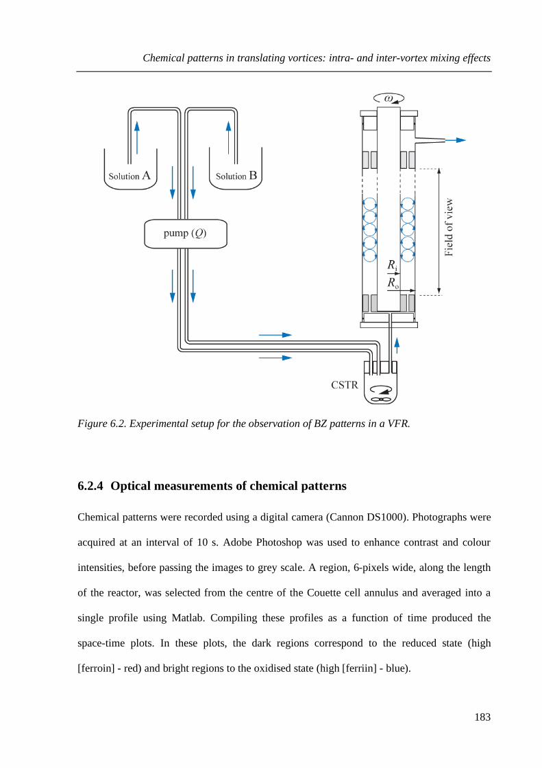
Chemical patterns in translating vortices: intra- and inter-vortex mixing effects

183

Figure 6.2. Experimental setup for the observation of BZ patterns in a VFR.

6.2.4 Optical measurements of chemical patterns

Chemical patterns were recorded using a digital camera (Cannon DS1000). Photographs were

acquired at an interval of 10 s. Adobe Photoshop was used to enhance contrast and colour

intensities, before passing the images to grey scale. A region, 6-pixels wide, along the length

of the reactor, was selected from the centre of the Couette cell annulus and averaged into a

single profile using Matlab. Compiling these profiles as a function of time produced the

space-time plots. In these plots, the dark regions correspond to the reduced state (high

[ferroin] - red) and bright regions to the oxidised state (high [ferriin] - blue).

Chemical patterns in translating vortices: intra- and inter-vortex mixing effects

184

6.2.5 Parameter ranges

The viscosity of the solution, ν, was of 1.04 mm2 s−1 at 22 ± 0.5 ˚C, measured using a

calibrated Ubbelohde viscometer. Four evenly spaced rotation rate values, ω, were used, from

1 Hz to 2.5 Hz. The Ta values varied from 17 to 43 for VFRH and between 16 and 41 for

VFRL. The flow rate varied between 4 cm3 min−1 and 13.6 cm3 min−1 for VFRH and between

11.6 cm3 min−1 and 13.6 cm3 min−1 for VFRL. The Re values varied from 1.7 to 5.3 for VFRH

and from 5.2 to 6.2 for VFRL. γRe = Uax / Riω varied from 0.03 to 0.29 for VFRH and from

0.13 to 0.39 for VFRL. Each experiment was repeated a minimum of three times.

For VFRL, the translational velocity of the vortices, UTV, was measured using a dye-

visualisation method. A sulphuric acid solution ([H2SO4] = 0.13 M) having the same viscosity

as the ferroin-catalyzed BZ reaction was pumped into the reactor. Using the same viscosity as

the ferroin-catalysed BZ reaction enabled obtaining similar flow properties. Visualisation of

the vortices was achieved by injecting 0.5 ml of 25 mM ferroin solution at the inlet of the

pump. UTV was obtained by measuring the time taken by the vortices to travel a given

distance. Uax was measured during the filling of the reactor.

6.2.6 Modelling chemical pattern formation in travelling vortices

A model has been developed21 in collaboration with the group of Annette Taylor (School of

Chemistry, University of Leeds), to simulate the formation of chemical patterns in translating

vortex flow in a system where Vd ~1. The BZ reaction was modelled using a 2-variable

Oregonator model18,22. This model retains the dominant reactions of the FKN reaction

mechanism (cf. 1.3.2) and their rate constants kn. The model reactions can be expressed by a

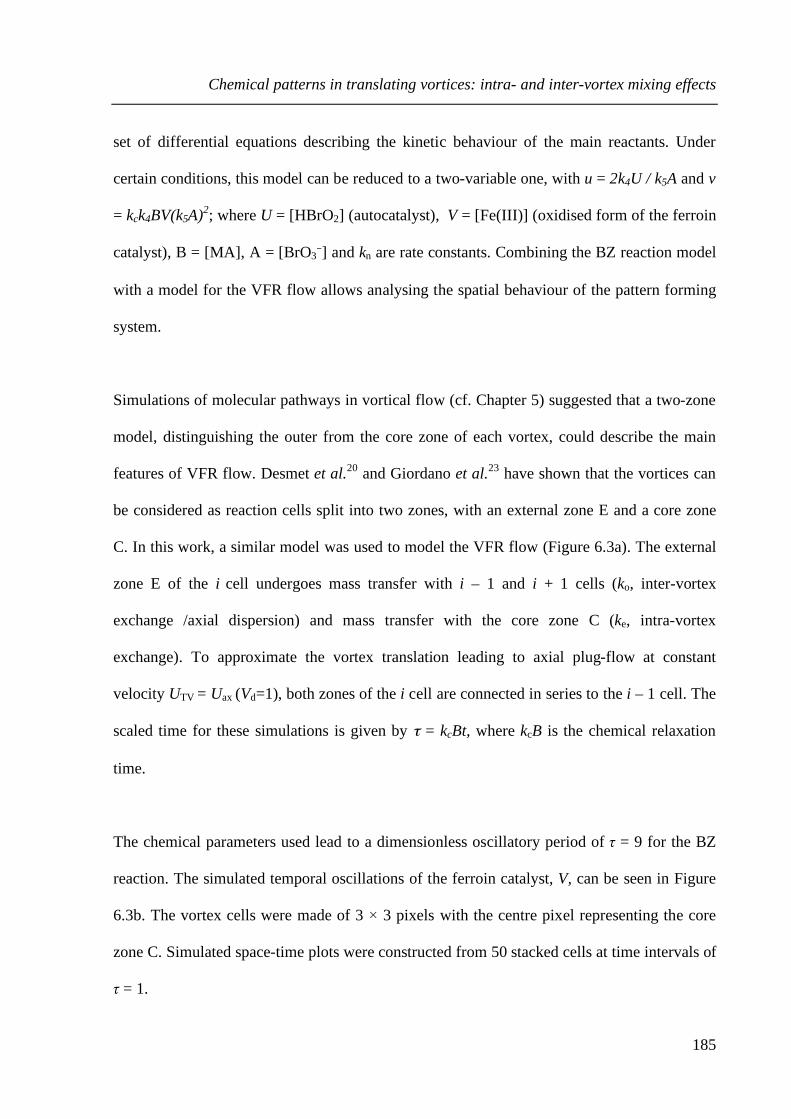
Chemical patterns in translating vortices: intra- and inter-vortex mixing effects

185

set of differential equations describing the kinetic behaviour of the main reactants. Under

certain conditions, this model can be reduced to a two-variable one, with u = 2k4U / k5A and v

= kck4BV(k5A)2; where U = [HBrO2] (autocatalyst), V = [Fe(III)] (oxidised form of the ferroin

catalyst), B = [MA], A = [BrO3−] and kn are rate constants. Combining the BZ reaction model

with a model for the VFR flow allows analysing the spatial behaviour of the pattern forming

system.

Simulations of molecular pathways in vortical flow (cf. Chapter 5) suggested that a two-zone

model, distinguishing the outer from the core zone of each vortex, could describe the main

features of VFR flow. Desmet et al.20 and Giordano et al.23 have shown that the vortices can

be considered as reaction cells split into two zones, with an external zone E and a core zone

C. In this work, a similar model was used to model the VFR flow (Figure 6.3a). The external

zone E of the i cell undergoes mass transfer with i – 1 and i + 1 cells (ko, inter-vortex

exchange /axial dispersion) and mass transfer with the core zone C (ke, intra-vortex

exchange). To approximate the vortex translation leading to axial plug-flow at constant

velocity UTV = Uax (Vd=1), both zones of the i cell are connected in series to the i – 1 cell. The

scaled time for these simulations is given by τ = kcBt, where kcB is the chemical relaxation

time.

The chemical parameters used lead to a dimensionless oscillatory period of τ = 9 for the BZ

reaction. The simulated temporal oscillations of the ferroin catalyst, V, can be seen in Figure

6.3b. The vortex cells were made of 3 × 3 pixels with the centre pixel representing the core

zone C. Simulated space-time plots were constructed from 50 stacked cells at time intervals of

τ = 1.

Chemical patterns in translating vortices: intra- and inter-vortex mixing effects

186

Figure 6.3. (a) Sketch of two-zone reaction cells (E = outer zone and C = core zone) and

processes used in the model. (b) Model of temporal oscillations in a cell in the absence of

flow/dispersion.

Development of this model required the introduction of additional dimensionless numbers

that characterised the chemistry and transport properties of the system. The Dakömhler

number, relating the BZ reaction timescale with the characteristic flow time, is given by Da =

kcBd /UTV, where d is the annular gap width (m) and UTV is the velocity of the translating cells

(m s−1). The scaled axial flow rate is given by 1 / Da = UTV / (kcBd). The Péclet number,

relating the rate of advection to the rate of dispersion, is given by Pe = UTVd / ko, where ko is

the inter-vortex exchange coefficient (m2 s−1). The inter-vortex exchange rate is given by 1 /

(PeDa) = ko / (kcBd2). The scaled intra-vortex exchange rate Ke = ke / kcB where ke is the intra-

vortex exchange rate (s−1). By introducing these parameters, the model allows to investigate

the effects of intra- and inter-vortex exchanges on the resulting patterns.

Chemical patterns in translating vortices: intra- and inter-vortex mixing effects

187

6.3 Results and discussion

6.3.1 Temporal oscillations in the BZ reaction

Figure 6.4 shows a plot of temporal oscillations in the ferroin-catalysed BZ reaction in a batch

reactor, observed over time. The periodic increase in potential indicates a switch of the

catalyst from red (Fe2+) to blue (Fe3+). For all experiments, the first five oscillations had an

average period of 185 ± 3 s at 22 ± 0.5 ˚C. By introducing the BZ reaction into the travelling

vortex flow of a VFR, these temporal oscillations are spatially distributed along the length of

the reactor, giving rise to chemical patterns.

Figure 6.4. Temporal oscillations of the redox potential in the BZ reaction.

Chemical patterns in translating vortices: intra- and inter-vortex mixing effects

188

6.3.2 Chemical patterns in a high inter-vortex exchange system

The BZ reactants were pumped into VFRH (Vd ~ 1.3) and images of chemical patterns were

acquired. The plug-like properties of the translating vortices distributed the chemical

oscillations along the length of the reactor leading to the formation of flow-distributed

oscillation (FDO) bands. Figure 6.5 shows a schematic diagram of a series of translating

vortices (a) in comparison with close-up pictures of a single FDO band appearing in blue (b).

Figure 6.5. (a) Schematic diagram of the VFR with translating vortices. The thick red line

represents a pixel slice selection for the creation of space-time plots. (b) close-up on the

complete width of the VFR for the first FDO band of the space-time plot between 900 s and

940 s and (c) complete space-time plot of FDO patterns for Q = 8.8 cm3 min−1 and ω = 1Hz.

Chemical patterns in translating vortices: intra- and inter-vortex mixing effects

189

Plotting the evolution of an averaged profile taken along the entire length of the reactor

(Figure 6.5a) allows observing the long-time behaviour of the system in a space-time plot

(Figure 6.5c). The blue bands, corresponding to high ferriin concentration regions, appear in

white on this plot.

The bands are formed via wave-splitting mechanism, where a part of the wave leaves the

reactor while the other settles at stationary position13. The average distance between the

centres of successive bands corresponds to wavelength of the FDO bands, λFDO. The

segmentation of the bands observed in the close-up pictures is also reflected in the space-time

plot, where stripes can be seen within each band. This segmentation is mainly due to phase

inhomogeneities between the core of the vortices and the high circulation outer-zones.

Information on the transport properties within VFRH can help understanding the resulting

chemical patterns. Hence, the chemical pattern formation in this system was studied at the

same flow and rotation rates as for the previous sections, so as to compare with previously

obtained results on the flow properties of VFRH (Chapters 4 and 5).

Figure 6.6 shows three space-time plots of chemical pattern formation at Q = 7.2 cm3 min−1

and ω = 1 Hz. At this regime, the system was unstable and repetitions gave a range of

outcomes. Figure 6.6a shows stationary FDOs maintained over 2 hours. In Figure 6.6b FDOs

are initially formed but the bands fail to settle at their steady position and the system switches

to travelling waves (TW). In Figure 6.6c the reverse phenomenon is observed, where

travelling waves are produced initially before the system reaches equilibrium, with successive

bands settling at a fixed position. For each repetition, when stationary bands are formed, λFDO

was found to be constant (λFDO ~ 8 cm).

Chemical patterns in translating vortices: intra- and inter-vortex mixing effects

190

Figure 6.6. Space-time plots at Q = 7.2 cm3 min−1 and ω = 1 Hz

The presence of travelling waves in this system could be related to several factors10 as

boundary conditions, critical flow rate or poor plug-flow properties. Changes in BZ phase at

the inlet of the reactor (0 cm) indicate an unstable boundary condition (Figure 6.6). This could

explain the observation of TW, as a stationary boundary is an important requirement for the

production of stationary FDOs. Oscillating boundary conditions were previously shown to

produce TW24. Note that stationary waves in this system coincide with a stationary boundary

condition at the reactor inlet, while travelling waves are preceded by an oscillating boundary.

On the other hand, TW could also be caused by the poor plug-flow properties for this regime

of the VFRH, presented in the previous chapter. Finally, observation of TW can be related to

Chemical patterns in translating vortices: intra- and inter-vortex mixing effects

191

the flow rate. Kinematic models show that unstable bands can be generated bellow a critical

flow rate value where the flow velocity is not high enough to resolve spatially the BZ

temporal oscillation12.

The complexity of the system and the low reproducibility of the experiments make it

impossible, at this stage, to draw conclusions so as to the conditions that generate travelling

waves. Studying the effect of the main flow parameters (flow, rotation and boundary) on the

resulting patterns could provide with a better understanding of the mechanisms involved in

the pattern formation and with answers concerning the nature of the observed bands.

6.3.2.1 Flow rate effect on the pattern formation

Space-time plots for different flow rates at ω = 1 Hz (Figure 6.7) provide with some insight

into the effect of flow rate on the pattern formation. At Q = 4 cm3 min−1 (Figure 6.7a) the

chemical patterns remain unstable with no stationary bands observed. At Q = 8.8 cm3 min−1

(Figure 6.7b) no travelling waves were observed over this experimental time and the

boundary was maintained at a fixed phase. However, after 2 hours, the position of the bands is

still decreasing, indicating that they are not settled at a stationary position. Considering the

instabilities observed at Q = 7.2 cm3 min−1 and the dynamic behaviour of the bands, no

conclusions should be drawn so as to the long-term stability of these chemical patterns. At Q

= 10.4 cm3 min−1 (Figure 6.7c) the bands systematically reach their equilibrium position after

approximately 500-700 s.

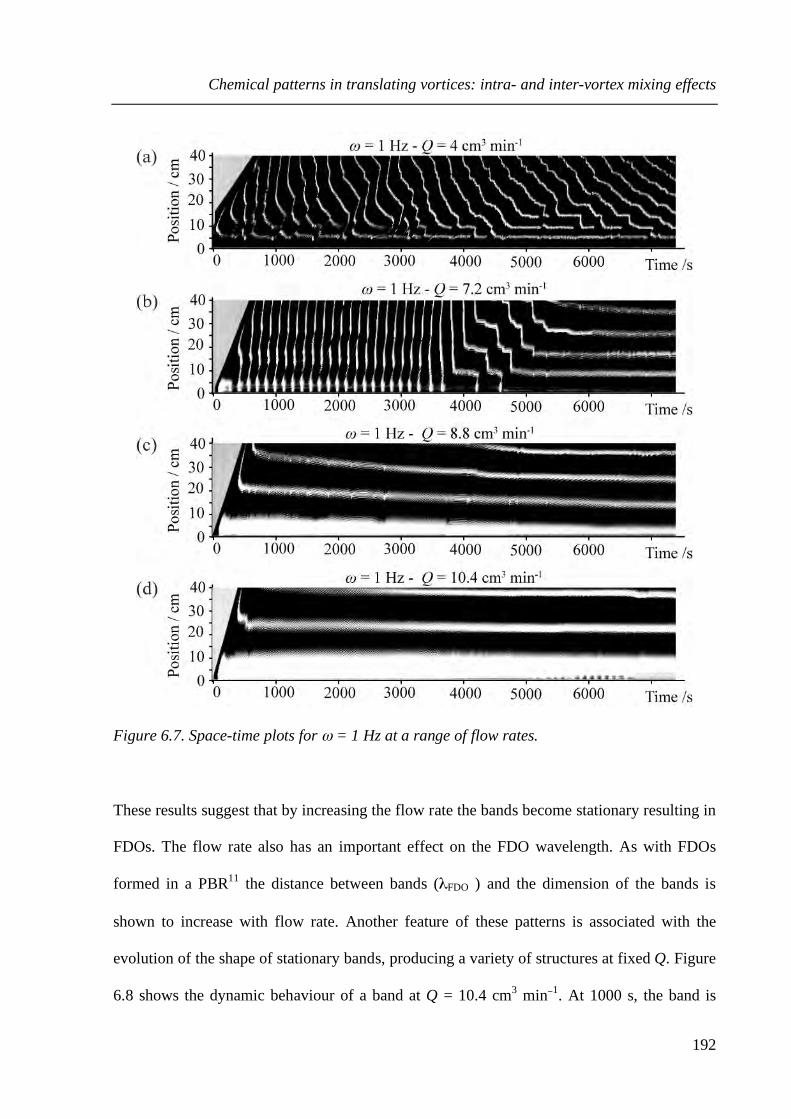
Chemical patterns in translating vortices: intra- and inter-vortex mixing effects

192

Figure 6.7. Space-time plots for ω = 1 Hz at a range of flow rates.

These results suggest that by increasing the flow rate the bands become stationary resulting in

FDOs. The flow rate also has an important effect on the FDO wavelength. As with FDOs

formed in a PBR11 the distance between bands (λFDO ) and the dimension of the bands is

shown to increase with flow rate. Another feature of these patterns is associated with the

evolution of the shape of stationary bands, producing a variety of structures at fixed Q. Figure

6.8 shows the dynamic behaviour of a band at Q = 10.4 cm3 min−1. At 1000 s, the band is

Chemical patterns in translating vortices: intra- and inter-vortex mixing effects

193

segmented, due to inhomogeneities between the core and the outer region of the vortices. As

the experiment advances, the band is progressively becoming more continuous. At 5000s the

band is uniform, with discontinuities only in the interface regions where the phase transition

occurs. At this stage, CO2 bubbles produced by the BZ reaction can be seen on the reactor

walls. This bubble production could not account for the dynamic behaviour of the band as it is

also a feature of lower flow rates, where different dynamic behaviour of the bands is

observed.

Figure 6.8. Close-up on the complete width of the VFR at different times for the first FDO

band of the space-time plot for Q = 10.4 cm3 min−1 and ω= 1Hz.

6.3.2.2 The role of the CSTR on the pattern formation

An investigation was performed on the role of the CSTR on the pattern formation. The use of

a CSTR is a standard feature of all experimental studies on FDOs using PBRs. It ensures that

a uniformly mixed solution is penetrating the reactor while maintaining a constant boundary

condition. However, the CSTR introduces additional parameters to the study of FDOs making

Chemical patterns in translating vortices: intra- and inter-vortex mixing effects

194

the analysis of the resulting pattern more complicated. A VFR flow provides with constant

mixing within the vortices, so the mixing of the reactants prior to the inlet of the reactor

provided by the CSTR becomes redundant. This was tested in a series of experiments at low

flow rates without CSTR.

At Q = 7.2 cm3 min−1, where travelling waves were observed in the presence of a CSTR

(Figure 6.6), all repetitions without CSTR produced stationary FDOs (Figure 6.9a).

Figure 6.9. Space-time plots of a system without CSTR for ω = 1 Hz at Q = 7.2 cm3 min−1 (a)

and Q = 4 cm3 min−1(b).

This suggests that the instabilities observed in the experiments with CSTR were caused by the

CSTR oscillations. At Q = 4 cm3 min−1, despite the stationary boundary, no stationary bands

were observed. It can be concluded that the critical flow rate for the formation of FDOs is

found between 4 cm3 min−1 and 7.2 cm3 min−1. These results demonstrate that the presence of

Chemical patterns in translating vortices: intra- and inter-vortex mixing effects

195

the CSTR might play a crucial role in determining the resulting patterns at low flow rates. It

can introduce difficulties in the analysis of the system, where instabilities of the CSTR might

be confounded with a critical flow rate regime. Note that previous experimental studies of

pattern formation13,25, used CSTRs of different dimensions, and probably different mixing

properties.

6.3.2.3 Rotation rate effect on the pattern formation

The rotation rate is the new parameter in the study of chemical pattern formation that is

introduced by the use of the VFR. In the previous chapters, the rotation rate was found to play

an important role in determining the mixing properties of the reactor, with an increase in

rotation leading to higher mixing.

Figure 6.10 shows space-time plots for increasing rotation rates.

Figure 6.10 Space-time plots for Q = 7.2 cm3 min−1 at ω = 1.5 Hz (a) and ω = 2 Hz (b).

Chemical patterns in translating vortices: intra- and inter-vortex mixing effects

196

At ω = 1.5 Hz, stable FDOs are formed but the bands close to the outlet are found to be

thinner and more unstable. At ω = 2 Hz, FDOs seem to form via convective instability (CI-

FDOs), where series of bands fail to stabilise before one of them settles at a stationary

position. Note that contrary to the travelling waves observed at ω = 1 Hz (Figure 6.6b,c),

these CI-FDO are reproducible and always lead to the formation of stationary bands. Also, the

unstable bands in CI-FDO are generated at the top of the reactor while TW were linked with

instabilities at the inlet.

Figure 6.11 shows space-time plots for experiments at Q = 13.6 cm3 min−1 for different ω.

Figure 6.11 Space-time plots for Q = 13.6 cm3 min−1 at a range of rotation rates.

Chemical patterns in translating vortices: intra- and inter-vortex mixing effects

197

At this flow rate, boundary conditions are stable, allowing to study the effect of rotation on

stable FDOs. Stable FDO bands were obtained for this range of rotation rates. At ω = 1 Hz

(Figure 6.11a) the bands appear segmented while for ω > 1 Hz continuous bands are

observed. As the rotation rate increases the bands become unstable but no travelling waves

are observed. This instability could be attributed to increasing mixing or possibly enhanced

wobbling of the inner cylinder observed for ω > 2 Hz.

Care is required in interpreting the space-time plots at high rotation rates due to the wobbling

of the inner cylinder. Nevertheless, these results confirm that stable FDOs could be obtained

in a high inter-vortex mixing VFR for a significant range of parameters. The relative roles of

rotation and flow rate need to be further studied. The chemical patterns resulting from each

set of parameters ω and Q were shown to be strongly dependant on the flow properties. The

observation of CI-FDOs at high rotation rates shows that inter- and intra-vortex mixing

effects play a crucial role in determining the features of the resulting chemical patterns. A

systematic study of intra- and inter-vortex mixing effects of chemical pattern formation in a

VFR was conducted using a second reactor, VFRL, that has better plug flow properties (Vd ~

1) and exhibits reduced wobbling at higher rotation rates.

6.3.3 Chemical patterns in a low inter-vortex exchange system

The dye experiments were used to probe the plug-flow properties of VFRL. The velocity drift,

Vd = UTV / Uax, was found to vary between 1 and 1.1, suggesting low inter-vortex mixing. As

for previous results (cf. 4.3.3), higher Vd values were obtained at lower rotation rates.

Chemical pattern formation in this system was studied at the same range of parameters as the

dye experiments. In order to study the relative effect of flow and rotation rates on the

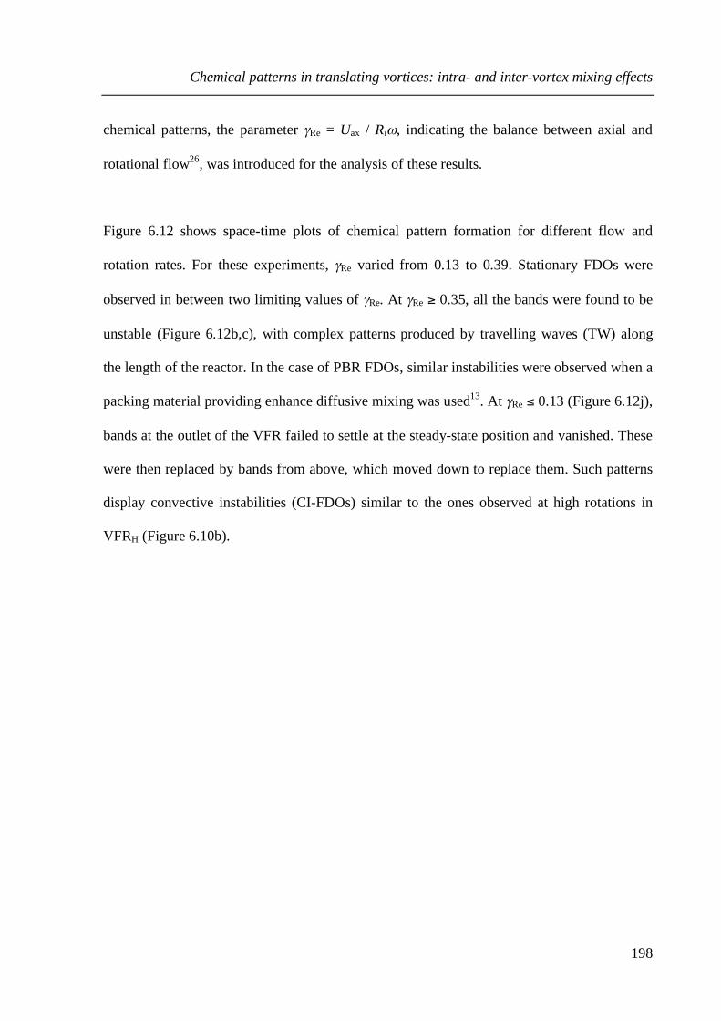
Chemical patterns in translating vortices: intra- and inter-vortex mixing effects

198

chemical patterns, the parameter γRe = Uax / Riω, indicating the balance between axial and

rotational flow26, was introduced for the analysis of these results.

Figure 6.12 shows space-time plots of chemical pattern formation for different flow and

rotation rates. For these experiments, γRe varied from 0.13 to 0.39. Stationary FDOs were

observed in between two limiting values of γRe. At γRe ≥ 0.35, all the bands were found to be

unstable (Figure 6.12b,c), with complex patterns produced by travelling waves (TW) along

the length of the reactor. In the case of PBR FDOs, similar instabilities were observed when a

packing material providing enhance diffusive mixing was used13. At γRe ≤ 0.13 (Figure 6.12j),

bands at the outlet of the VFR failed to settle at the steady-state position and vanished. These

were then replaced by bands from above, which moved down to replace them. Such patterns

display convective instabilities (CI-FDOs) similar to the ones observed at high rotations in

VFRH (Figure 6.10b).

Chemical patterns in translating vortices: intra- and inter-vortex mixing effects

199

Figure 6.12. (a-l) Space-time plots at a range of flow and rotation rates.

Chemical patterns in translating vortices: intra- and inter-vortex mixing effects

200

The phase diagram in Figure 6.13 summarises the variety of patterns observed in this system,

as a function of Q and ω.

Figure 6.13. Phase diagram of patterns observed as function of flow and rotation rates. The

arrow indicates the transition from lower to higher γRe values. Doted lines indicate phase

transitions.

For all stable FDOs, λFDO was found to increase with flow rate (Figure 6.14) and the rotation

rate only seems to have an effect on λFDO at higher flow rates. These results are similar to

those observer in FDO studies in a PBR12−14, where the distance between bands increases with

the flow rate. At lower γRe the bands are found to be solid (Figure 6.12j-l), while at higher γRe

they have a segmented structure, appearing as stripes within a band on the space-time plot

(Figure 6.12a-c). Segmentation of the bands seems to be related to the poor mixing properties

of the reactor, since it has been a common feature of the chemical patterns in the high inter-

vortex mixing VFR (Figure 6.5, Figure 6.6, Figure 6.7).

Chemical patterns in translating vortices: intra- and inter-vortex mixing effects

201

Figure 6.14. Plot of the average distance between stable FDO bands against flow rate for ω=

1.5 Hz (---), ω = 2 Hz (···) and ω = 2.5 Hz (—).

Closer inspection of the chemical bands provides insight into the structure and possible

formation mechanisms. Figure 6.15 shows close-up photos of a FDO band at Q = 11.6 cm3

min−1, for different rotation rates.

Figure 6.15. Digital photographs of the second FDO band from the inlet at Q = 11.6 cm3 min–

1 and for increasing rotation rate: ω = 1 Hz (a), ω = 1.5 Hz (b), ω = 2 Hz (c) and ω = 2.5 Hz

(d). The dimension of one vortex pair, λ, is indicated in (a).

Chemical patterns in translating vortices: intra- and inter-vortex mixing effects

202

At low ω (Figure 6.15a,b), there appears to be a heterogeneous distribution of the oxidised

state between neighbouring vortices, as well as between the centre region of the vortices and

the outside region. This heterogeneous distribution gives rise to the segmented bands

observed on the space-time plots (Figure 6.12a). At constant flow rate, an increase in rotation

rate was found to lead to the progressive disappearance of the segmented bands (Figure

6.15c,d) and the formation of a homogeneous distribution of oxidised and reduced states, with

narrower and more clearly defined bands.

The resulting chemical patterns are shown to depend strongly on the interplay between

chemistry and inter- and intra-vortex mixing. Comparison of the experimental chemical

pattern features with simulations combining the Oregonator model for the BZ reaction with a

VFR flow model were performed to get a better understanding of the mechanisms underlying

the coupling between oscillating reactions and vortical flow.

6.3.4 Inter- and intra-vortex mixing effects

Simulations were used to explore the effects of flow rate, inter-vortex exchange rate and intra-

vortex exchange rate on the resulting patterns. In order for the model to provide some

illumination regarding the experimental results it was necessary to link the parameters used in

each case. The increase of the rotation rate (ω) in a VFR has been shown to increase both

intra-vortex mixing (ke) and inter-vortex mixing (ko) through dispersion23,27. For relatively

low rotation rates, an increase of the flow rate (Q) has also been shown to increase inter-

vortex mixing28. Flow-induced inter-vortex mixing is linked with the formation of high

circulation paths on the outer zones of successive vortices. For low intra-vortex mixing, these

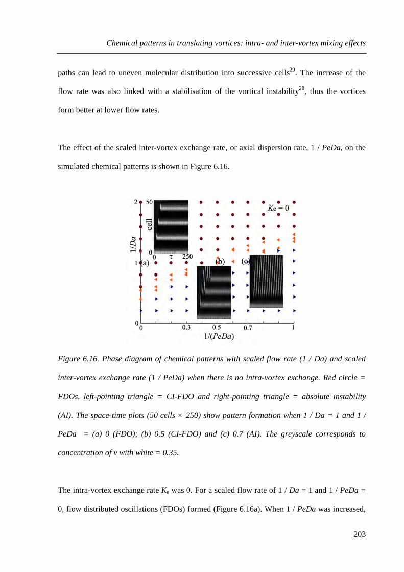
Chemical patterns in translating vortices: intra- and inter-vortex mixing effects

203

paths can lead to uneven molecular distribution into successive cells29. The increase of the

flow rate was also linked with a stabilisation of the vortical instability28, thus the vortices

form better at lower flow rates.

The effect of the scaled inter-vortex exchange rate, or axial dispersion rate, 1 / PeDa, on the

simulated chemical patterns is shown in Figure 6.16.

Figure 6.16. Phase diagram of chemical patterns with scaled flow rate (1 / Da) and scaled

inter-vortex exchange rate (1 / PeDa) when there is no intra-vortex exchange. Red circle =

FDOs, left-pointing triangle = CI-FDO and right-pointing triangle = absolute instability

(AI). The space-time plots (50 cells × 250) show pattern formation when 1 / Da = 1 and 1 /

PeDa = (a) 0 (FDO); (b) 0.5 (CI-FDO) and (c) 0.7 (AI). The greyscale corresponds to

concentration of v with white = 0.35.

The intra-vortex exchange rate Ke was 0. For a scaled flow rate of 1 / Da = 1 and 1 / PeDa =

0, flow distributed oscillations (FDOs) formed (Figure 6.16a). When 1 / PeDa was increased,

Chemical patterns in translating vortices: intra- and inter-vortex mixing effects

204

the FDOs formed via a convective instability, where initial perturbations were amplified with

the flow (Figure 6.16b). Above a critical value of 1 / PeDa, absolute instabilities (AI) were

observed, where the spatial oscillation transformed into a temporal one (Figure 6.16c). AI

appear as travelling waves along the length of the reactor.

These simulations reproduce the main features of the experimental chemical pattern

observation (FDOs, CI-FDOs and TW). The simulation results suggest that the instabilities

obtained experimentally at low and high γRe values are generated by enhanced inter-vortex

mixing. Inter-vortex mixing at low rotation rates, where travelling waves were observed

(Figure 6.12b,c), seems to be higher than inter-vortex mixing at high rotation rates, where CI-

FDOs are observed (Figure 6.12j).

Simulation results at a fixed flow rate, illustrate the influence of intra-vortex exchange on the

patterns (Figure 6.17). With a scaled intra-vortex exchange rate of Ke = 0.2, there was a phase

lag between the outer zone and core zone of the vortices with the FDO band beginning in the

outer region. The critical inter-vortex exchange rate for the CI-FDO and the AI was increased

compared to in the absence of intra-vortex exchange. When Ke was increased to 1.2, the phase

lag between the outer and core zone disappeared and narrower bands were observed. Also, the

transition to CI-FDO and AI occurred at even higher values of 1 / PeDa. These results are in

good agreement with experimental chemical pattern formation observations. The segmented

bands observed at low rotation rates both for high and low inter-vortex exchange systems

(Figure 6.6 and Figure 6.12a respectively) can be attributed to low intra-vortex exchange

cases. At the higher rotation rates, where increased intra-vortex mixing occurs, the bands were

also found to be narrower (Figure 6.15). In the simulations, when the dispersion in the outer-

Chemical patterns in translating vortices: intra- and inter-vortex mixing effects

205

region is sufficient to cause absolute instabilities, coupling with the inner core can lead to

convective instabilities and then back to stable FDOs. In the experiment, the travelling waves

observed at ω = 1 Hz at high flow rates (Figure 6.12b,c) can be stabilized by increasing the

rotation rate and, hence, the intra-vortex mixing (Figure 6.12e,f). But in this case, rotation

also affects the inter-vortex mixing, so no conclusions can be drawn.

Figure 6.17. Simulated space-time plots showing the critical dispersion rate 1 / PeDa for the

appearance of convective and absolute instabilities at different intra-vortex exchange rates,

Ke. The scaled flow rate, 1 / Da, was 1.

Additional information on the stabilising role of intra-vortex mixing is provided by simulation

results where the flow and the inter-vortex exchange rate are increased simultaneously

(Figure. 6.18). For low intra-vortex exchange rates, the increase of flow and inter-vortex

exchange is followed by a transition from FDOs to travelling waves (AI). An increase in the

intra-vortex-exchange rate, Ke, led to the re-emergence of stable FDO. These results can also

be related to the experimental ones. An increase of flow rate (inter-vortex mixing) between

Chemical patterns in translating vortices: intra- and inter-vortex mixing effects

206

Figure 6.12a and Figure 6.12b led to TW, while an increase in rotation (intra-vortex mixing)

between Figure 6.12b and Figure 6.12e led to the formation of stable FDOs.

Figure. 6.18. Simulated space-time plots showing the effect of increasing flow rate and inter-

vortex exchange rate on the patterns at two different intra-vortex exchange rates.

6.4 Conclusions

The results shown in this chapter demonstrate that flow distributed oscillations (FDOs) can

form over a significant range of parameters, despite the travelling vortex flow complexity and

high inter-vortex mixing.

Similarities with FDOs observed in PBRs12−14 were identified, as the band distance increase

with flow rate and the existence of a critical flow rate for the stabilisation of the bands. In a

VFR, high mixing inside the vortices was shown to make the CSTR redundant. Removing it

allowed reducing the minimum flow rate for stable FDO observation. FDOs in a VFR become

Chemical patterns in translating vortices: intra- and inter-vortex mixing effects

207

unstable as the flow rate Q is increased at low rotation rates, with the observation of complex

patterns and travelling waves. This was attributed to increased inter-vortex mixing. In the

PBR, similar instabilities were observed when the packing material was changed to enhance

diffusive mixing13. At high rotation rates, FDOs in a VFR were shown to form via convective

instability, where successive bands fail to settle at equilibrium position before the stationary

pattern is observed. Similar structures were observed at low flow rates in the PBR13 and

increasing the flow rate could stabilise the FDO bands.

Simulations combining the Oregonator model for the BZ reaction with a model considering

cells with an inner vortex core coupled to an outer zone reproduced the main features of the

system. Comparison between experimental and simulated results of pattern formation allowed

the effect of inter-vortex and intra-vortex mixing of to be studied. The simulations showed

that above a critical inter-vortex exchange rate, 1/ PeDa, the FDO bands tend to become

unstable and absolute instabilities (AI) appear forming travelling waves similar to the ones

observed in the experiments. The disappearance of bands observed at high rotation and low

flow rates appears to be related to the convective instabilities observed in the simulations as

the inter-vortex exchange rate is increased: the perturbations are amplified upstream resulting

in the loss of FDO band stability. Flow or rotation induced inter-vortex mixing can destabilise

stationary FDO patterns because of dispersive mixing. However, the coupling of the vortex

core with the outer zone can lead to the re-appearance of stable FDOs. The agreement of

experimental and simulated results suggests that exploring the interplay between modes of

pattern formation in a VFR for bigger ranges of parameters may provide insight into more

complex instabilities observed in networks of coupled cellular systems30−33.

Chemical patterns in translating vortices: intra- and inter-vortex mixing effects

208

(1) De Wit, A.; Eckert, K.; Kalliadasis, S. Chaos 2012, 22.

(2) Tel, T.; de Moura, A.; Grebogi, C.; Karolyi, G. Phys. Rep. 2005, 413, 91.

(3) Vladimirova, N.; Constantin, P.; Kiselev, A.; Ruchayskiy, O.; Ryzhik, L.

Combust. Theor. Model. 2003, 7, 487.

(4) Kiss, I. Z.; Merkin, J. H.; Scott, S. K.; Simon, P. L.; Kalliadasis, S.; Neufeld,

Z. Physica D 2003, 176, 67.

(5) Medvinsky, A. B.; Petrovskii, S. V.; Tikhonova, I. A.; Malchow, H.; Li, B. L.

Siam Rev. 2002, 44, 311.

(6) Neufeld, Z. Chaos 2012, 22.

(7) Steinbock, O.; Siegert, F.; Muller, S. C.; Weijer, C. J. P. Natl. Acad. Sci. USA

1993, 90, 7332.

(8) Perumpanani, A. J.; Sherratt, J. A.; Maini, P. K. Ima J. Appl. Math. 1995, 55,

19.

(9) Mcgraw, P. N.; Menzinger, M. Phys. Rev. E 2003, 68.

(10) Andresen, P.; Bache, M.; Mosekilde, E.; Dewel, G.; Borckmans, P. Phys. Rev.

E 1999, 60, 297.

(11) Kaern, M.; Menzinger, M. Phys. Rev. E 1999, 60, R3471.

(12) Bamforth, J. R.; Toth, R.; Gaspar, V.; Scott, S. K. Phys. Chem. Chem. Phys.

2002, 4, 1299.

(13) Taylor, A. F.; Bamforth, J. R.; Bardsley, P. Phys. Chem. Chem. Phys. 2002, 4,

5640.

(14) Britton, M. M.; Sederman, A. J.; Taylor, A. F.; Scott, S. K.; Gladden, L. F. J.

Phys. Chem. A 2005, 109, 8306.

Chemical patterns in translating vortices: intra- and inter-vortex mixing effects

209

(15) Novak, J. Visualisation of Chemistry in Flow, University of Birmingham,

2010.

(16) Taylor, A. F.; Britton, M. M. Chaos 2006, 16.

(17) Pocheau, A.; Harambat, F. Phys. Rev. E 2006, 73.

(18) Thompson, B. W.; Novak, J.; Wilson, M. C. T.; Britton, M. M.; Taylor, A. F.

Phys. Rev. E 2010, 81.

(19) Paoletti, M. S.; Solomon, T. H. Phys. Rev. E 2005, 72.

(20) Desmet, G.; Verelst, H.; Baron, G. V. Chem. Eng. Sci. 1996, 51, 1287.

(21) Vallatos, A.; Evans, R. D.; Taylor, A. F.; Britton, M. M. Chaos 2013, 23.

(22) Bamforth, J. R.; Merkin, J. H.; Scott, S. K.; Toth, R.; Gaspar, V. Phys. Chem.

Chem. Phys. 2001, 3, 1435.

(23) Giordano, R. L. C.; Giordano, R. C.; Prazeres, D. M. F.; Cooney, C. L. Chem.

Eng. Sci. 2000, 55, 3611.

(24) Kaern, M.; Menzinger, M. Phys. Rev. E 2000, 61, 3334.

(25) Kaern, M.; Menzinger, M. J. Phys. Chem. A 2002, 106, 4897.

(26) Gu, Z. H.; Fahidy, T. Z. Can. J. Chem. Eng. 1985, 63, 710.

(27) Giordano, R. C.; Giordano, R. L. C.; Prazeres, D. M. F.; Cooney, C. L. Chem.

Eng. Sci. 1998, 53, 3635.

(28) Wereley, S. T.; Lueptow, R. M. Phys. Fluids 1999, 11, 3637.

(29) Vallatos, A.; Wilson, M. C. T.; Taylor, A. F.; Britton, M. M. Europhys. Lett.

2012.

(30) Votrubova, V.; Hasal, P.; Schreiberova, L.; Marek, M. J. Phys. Chem. A 1998,

102, 1318.

(31) Yoshimoto, M.; Yoshikawa, K.; Mori, Y. Phys. Rev. E 1993, 47, 864.

Chemical patterns in translating vortices: intra- and inter-vortex mixing effects

210

(32) Nevoral, V.; Votrubova, V.; Hasal, P.; Schreiberova, L.; Marek, M. J. Phys.

Chem. A 1997, 101, 4954.

(33) Laplante, J. P.; Erneux, T. Physica A 1992, 188, 89.

MR Imaging of chemical waves in vortical flow

211

7 MR Imaging of chemical waves in vortical flow

7.1 Introduction

In the previous chapter, the analysis of chemical pattern formation arising from the coupling

of oscillating reactions and vortical flow was shown to provide information on flow

properties, such as inter- and intra-vortex mixing. Molecular displacements within the flow

are expected to play an important role in determining the features of the propagating chemical

waves.

MRI studies of BZ waves in stationary and travelling vortex flow were performed to get a

better understanding of the interplay between reaction and transport in these systems. The

characteristics of the chemical waves were analysed in the light of previously presented

results on the molecular transport properties of the flows. Three types of systems presenting

different features were investigated: travelling waves in stationary vortices, travelling waves

in travelling vortices and stationary waves in travelling vortices (FDOs). This work

demonstrates how magnetic resonance experiments can provide deeper insight into

underpinning mechanisms behind pattern forming RDA systems, particularly those involving

vortical flows.

In order to image chemical waves using MRI, the manganese-catalysed BZ reaction was used.

Contrary to the ferroin catalyst1 used in the previous chapter, manganese has been shown to

provide good MR contrast2 between the two oxidative states (Mn3+ and Mn2+). On the other

hand, poor optical contrast is obtained with manganese-catalysed BZ systems3. But optical

MR Imaging of chemical waves in vortical flow

212

contrast was necessary in order to visualise the overall chemical pattern formation and make

sure that stationary waves formed within the MRI rf coil, in a region of about 4 cm. Also, in

order to obtain stationary waves within the VFR, the oscillation period of the manganese

catalysed BZ reaction had to be similar to the one of the ferroin-catalysed BZ reaction used in

the previous chapter.

In initial publications4,5 on MRI of the manganese-catalysed BZ reaction, high concentrations

of phosphoric acid (H3PO4) were used (> 1 M). The phosphate group (PO43−) of phosphoric

acid was shown to improve MR contrast by stabilising the Mn3+ ions6. In previous MR studies

of FDOs in a PBR, Britton et al.7 also used a version of the manganese-catalysed BZ reaction

involving high concentrations of sulphuric and phosphoric acid. Thompson et al.8 used the

same reaction to visualise BZ waves propagating in stationary vortices. But high acid

concentrations lead to high-viscosity solutions9, which are significantly higher than those

used in the previous chapters of this thesis to characterise vortical flows. Thus, a manganese-

catalysed BZ reaction of similar viscosity had to be used, so as to ensure similar flow

properties. In order to obtain lower viscosity solutions, the phosphoric acid was replaced with

Na5P3O10, which has been shown6 to also stabilise Mn3+. Moreover, Na5P3O10 allows to

produce a reaction of adaptable oscillation period without changing the flow properties of the

system10.

The MR contrast properties of oscillating chemistry and vortical flow were analysed

separately, prior to the imaging of chemical waves in vortical flow. Chemical contrast was

studied using MRI of phantom samples containing an oxidised and a reduced form of the BZ

reaction6, in order to evaluate the maximum contrast expected for each set of parameters. The

MR Imaging of chemical waves in vortical flow

213

imaging parameter ranges were restricted to values leading to short sequence times, in order

to take into account the transient nature of the chemical waves and the effects of flow. MR

imaging sequences have been shown to be subject to flow artifacts11,12. Also, T1 and T2

relaxation times used for MRI contrast are sensitive to molecular motion and flow

properties13. Experiments were conducted to study the effects of stationary and travelling

vortex flow on both MR relaxation and MR imaging.

The optimised manganese-catalysed BZ reaction and MR parameters were used to produce

images of chemical waves in vortical flow. Particular attention was given to the role of flow

properties, as intra- and inter-vortex mixing, on the propagation of the chemical waves.

Trying to separate flow- from chemistry-induced effects, the chemical wave images were

compared with molecular displacement simulations obtained in Chapter 5, at the same flow

regimes. The use of BZ reactions with different concentrations of manganese allowed

analysing the role of the catalyst into the wave propagation and opening a discussion on the

role of chemistry in the resulting pattern formation.

7.2 Experimental

7.2.1 The manganese-catalysed BZ reaction

The manganese-catalyzed BZ reaction was prepared immediately before each experiment

using reactants dissolved in deionized water. Solution A contained malonic acid ([MA] = 0.5

M, Alfa Aesar, 99 %) and sodium bromate ([BrO3–] = 0.14 M, Alfa Aesar, 99.5 %). Solution

B contained sulfuric acid ([H2SO4] = 1 M, Fisher, 98 %), penta-sodium triphosphate

MR Imaging of chemical waves in vortical flow

214

([Na5P3O10] = 4 mM, Sigma Aldrich, 98%) and the manganese catalyst (Sigma Aldrich,

98%). [MnSO4] varied from 0.5 mM to 8 mM. Solutions A and B were degassed prior to

experimentation.

Control solutions of either the oxidised or reduced state of the BZ reaction were obtained by

removing one of the main reactants (MA or BrO3–) of the mixed BZ solution6. The oxidised

state solution contained sodium bromate ([BrO3–] = 0.07 M), sulfuric acid ([H2SO4] = 0.5 M),

penta-sodium triphosphate ([Na5P3O10] = 2 mM) and the manganese catalyst. The reduced

state solution contained malonic acid ([MA] = 0.25 M), sulfuric acid ([H2SO4] = 0.5 M),

penta-sodium triphosphate ([Na5P3O10] = 2 mM) and the manganese catalyst. For both

solutions [MnSO4] varied from 0.25 mM to 4 mM.

7.2.2 Pt-electrode measurements of BZ temporal oscillations

Temporal oscillations were monitored in a well-stirred batch reactor using a Pt-combination

redox electrode connected to a Picoscope Oscilloscope (Picotech). The reaction temperature

was maintained at 22 ˚C ± 0.5 ˚C. The experimental set-up was the same as the one described

in section 6.2.2.

7.2.3 Experimental set-up for chemical waves in vortical flow

The Couette cell used was the same as the one described in the previous chapters, and

constructed from an outer glass tube of radius Ro = 8.25 mm and an inner PEEK rod of radius

Ri = 4.1 mm. Description of the experimental set-up for the observation of chemical patterns

MR Imaging of chemical waves in vortical flow

215

is detailled in Chapter 6 (cf. 6.2.3). For MR imaging experiments, the Couette cell was placed

in the MRI magnet, inside the rf coil. The coil was situated 11 cm above the lower PTFE

guide (cf. 4.2.1).

7.2.4 Flow parameter ranges

Tap water, of viscosity ν = 0.979 mm2 s−1 at 22 ± 0.5 ˚C, was used for the investigation into

flow artifacts. The manganese-catalysed BZ reaction was used for all the other experiments,

and had a viscosity of ν = 1.05 mm2 s−1 at 22 ± 0.5 ˚C. Viscosities were measured using a

calibrated Ubbelohde Viscometer. Four rotation rate values, ω, were used: 1 Hz, 1.5 Hz, 2 Hz

and 2.5 Hz. The respective Ta values varied from 17 to 43. For the pipe flow and translating

vortex flow experiments, two flow rate values, Q, were used: 7.2 cm3 min−1 and 13.6 cm3

min−1. The respective Re values were of 2.51 and 5.3. The velocity of translation of the

vortices, UTV, varied between 0.45 mm s-1 and 1.51 mm s-1 and the velocity drift, Vd, between

1.02 and 1.21. γRe varied from 0.06 to 0.29. Each experiment was repeated a minimum of

three times.

7.2.5 Optical measurements

Optical images were acquired using a digital CCD camera (Canon Power Shot A520). Adobe

Photoshop was used to enhance colour contrast. The pink colour component of each image

was saturated, so that the pink solutions, where Mn3+ predominated, could be distinguished

from the colourless solutions, where Mn2+ predominated. Chemical pattern formation images

were passed to grey scale with the pink components (Mn3+) appearing in black and the

MR Imaging of chemical waves in vortical flow

216

colourless components (Mn2+) in white. Space-time plots of chemical pattern formation were

produced using the method presented in Chapter 6 (cf. 6.2.4).

7.2.6 T1 and T2 relaxation measurements

T1 and T2 relaxation times of both oxidised and reduced solutions were measured for [Mn]

values of 0.25 mM, 0.5 mM, 1 mM, 2 mM and 4 mM. T1 relaxation times were measured

using an inversion-recovery sequence (Figure 2.4). Variable delay lists with 20 exponentially

spaced τ values were used (from 5×10−6 s to 1 s, 2 s, 5 s or 10 s). T2 relaxation times were

measured using a CPMG sequence (Figure 2.6). A series of 17 spectra were collected,

acquired using a range of echoes. A variable count list was used with values ranging from 0 to

1500. The echo time, τ, was varied between 0.5 ms and 3 ms.

For both inversion recovery and CPMG experiments, the spectral width was 10 kHz and 16 k

complex data points were acquired. Four signal averages were acquired for each τ value. The

hard rf pulse length was of 45 µs for the 90° r.f. pulse and 90 µs for the 180° r.f. pulse. The

data was analysed using Prospa and Kaleidagraph software.

Both experiments produced two-dimensional data sets of spectral data against points in the

variable delay (inversion recovery) or variable counter (CPMG) lists. For the inversion

recovery experiment data, the signal intensity against time was fitted to a single-exponential

recovery function (equation 2.1) to obtain the T1 value. For the CPMG data, the signal

intensity against time was fitted to a single-exponential decay function (equation 2.2) to

obtain the T2 value.

MR Imaging of chemical waves in vortical flow

217

7.2.7 Relaxation-weighted imaging

A phantom sample made from the oxidised and reduced state solutions of the BZ reaction was

used to determine the imaging parameters that produce the higher contrast. These parameters

were used to image chemical waves in the Couette cell.

For the phantom sample experiments, a 5 mm o.d. NMR tube filled with the oxidised state

solution (Mn3+) was placed inside a 10 mm o.d. tube filled with the reduced state BZ solution

(Mn2+) (Figure 7.1a). The tubes were then placed inside the probe, in the MRI magnet.

Images were acquired in the transversal plane so as to visualise the cross section of the tubes

(Figure 7.1b). For this experiments, the field of view was of 2 cm2 with a matrix size of 128 ×

128 pixels.

Figure 7.1. (a) Schematic diagram of the experimental set-up for phantom experiments. (b)

Transverse section of the image in (a) at the level indicated by the arrows.

For imaging chemical waves within the Couette cell, the field of view was 40 × 20 mm with a

matrix size of 128 × 64 pixels resulting in a pixel size of 0.3125 mm2. The cell was placed

into the magnet and the MRI field of view (rf coil) was situated 11 cm above the lower PTFE

MR Imaging of chemical waves in vortical flow

218

guide. The same set-up and parameters were used for studying flow-induced contrast in

imaging of tap water.

A spin echo imaging pulse sequence was used for all MR imaging experiments (Figure 2.11).

The soft rf pulse length was of 1 ms with attenuations of 8 - 13 dB for the 90° pulse and 2 - 7

dB for the 180° pulse. Spectral widths of 50 kHz and 100 kHz were used. A slice thickness of

1 mm was used. Recovery time, TR, between 100 ms and 300 ms. The echo time, TE, varied

between 3 ms and 35 ms. At this range of TR and TE, MR contrast was obtained with a

combination of T1- and T2-weighted contrast, with T1 contrast dominating at low TE and T2

contrast dominating at high TE.

MR Imaging of chemical waves in vortical flow

219

7.3 Results and discussion

7.3.1 Optical imaging of chemical patterns in translating vortices

In order to visualise optically the waves produced by the manganese-catalysed BZ reaction

one has to be able to distinguish between the oxidised and reduced states. In the Mn2+ / Mn3+

system, the reduced state (Mn2+) is colourless and the oxidised (Mn3+) is pink. The contrast

between the two states depends on [Mn]. But even if the manganese concentration is

sufficient to produce optical contrast in bulk solutions, when the solution layer is thin, poor

contrast is observed between the two states. However, it is possible to enhance optical

contrast either by changing the composition (increasing [Mn]) or by enhancing the image,

using an image-editing software. Figure 7.2a shows pictures of BZ solutions in 20 mm tubes

with increasing Mn3+ concentrations. For [Mn3+] = 0 the solution is colourless like the

reduced state solutions. The pink colour intensity is increasing with [Mn3+].

Figure 7.2 (a) Optical contrast at increasing [Mn3+] and (b) Photoshop enhanced optical

contrast for the same picture.

MR Imaging of chemical waves in vortical flow

220

In the Couette cell, where the gap (and the fluid column thickness) is of only 4.15 mm, the

contrast is poorer and the pink colouration is visible only for [Mn3+] ≥ 2 mM. To visualise

BZ contrast for [Mn3+] < 2 mM, Photoshop was used to saturate the pink component in the

images (Figure 7.2b). Using the BZ reaction in a Couette cell, no good contrast was obtained

for [Mn3+] = 0.25 mM. Very good contrast was obtained for [Mn3+] = 4 mM, but at this

manganese concentration, the BZ oscillations were producing a lot of CO2, perturbing the

pattern formation and reducing the imaging quality. Therefore, only BZ reactions with 0.5

mM ≤ [Mn3+] ≤ 2 mM were used for optical imaging experiments of chemical pattern

formation in translating vortex flow.

While changing [Mn] can improve the visualisation of the waves, there are also effects on the

BZ reaction. Pt-electrode measurements were performed to determine the oscillation period of

the BZ reaction for increasing [Mn3+]. Figure 7.2 shows plots of temporal oscillations in the

BZ reaction for three [Mn] observed over 30 minutes using the Pt-electrode. As the potential

oscillates, there is an oscillatory conversion between Mn2+ and Mn3+, with Mn2+ at low

potential and Mn3+ at high potential. The sharp increases in potential correspond to the

autocatalytic steps where the system switches from colourless (Mn2+) to pink (Mn3+). Each

potential maximum is followed by a slower decay that brings the system back to the reduced

state. Where [Mn] = 2 mM, there is an additional shoulder after each peak, indicating a

possible change in the behaviour of the BZ oscillation.

The average oscillation period was of 100 s for [Mn] = 0.5 mM, 170 s for [Mn] = 1 mM and

200 s for [Mn] = 2 mM. For comparison, the oscillation period of the ferroin-catalysed BZ

reaction studied in the previous chapter was of 185 s (Figure 6.3).

MR Imaging of chemical waves in vortical flow

221

Figure 7.3. (a-c) Pt-electrode measurements of temporal oscillations in the BZ reaction for

increasing Mn concentrations. The period T represents the average oscillation period over

the observation time.

To investigate FDOs in the manganese-catalysed reaction, BZ systems with different Mn

concentrations were pumped into the Couette cell at Q = 7.2 cm3 min−1 and ω = 1 Hz (Figure

7.4). The grey-scale allows for a better visualisation of the resulting pattern. Dark bands in the

space-time plots correspond high [Mn3+] (pink), while light grey areas correspond to high

[Mn2+] (colourless).

MR Imaging of chemical waves in vortical flow

222

Figure 7.4. Chemical pattern formation of the Mn-catalysed BZ reaction at ω = 1 Hz and Q =

7.2 cm3 min−1 for (a) [Mn] = 0.5 mM, (b) [Mn] = 1 mM and (c) [Mn] = 2 mM.

It was observed that stationary bands formed for all Mn concentrations at this flow regime.

For [Mn] = 0.5 mM (Figure 7.4a), the bands formed via a convective instability (CI-FDO).

This is probably due to the lower oscillation period of the reaction. For [Mn] ≥ 1 mM the

bands form via the FDO mechanism involving a single wave-splitting, where a part of the

wave leaves the reactor while the other settles at stationary position14.

MR Imaging of chemical waves in vortical flow

223

For [Mn] = 1 mM (Figure 7.4b), where the oscillation period is close to the previously studied

ferroin-catalysed BZ system, a similar λFDO was found (λFDO ~ 10 cm). For [Mn] = 2 mM, the

speed of the descending waves is found to decrease dramatically and the bands take more

time to settle to the stationary position. Almost 1 hour was required for the first band to settle.

Hence, 2-hour experiments were required to observe stationary bands at this Mn

concentration. During the wave-splitting, the distance between successive bands is greater

than for the lower Mn concentration systems. However, the resulting λFDO is found to be

shorter, although the oscillation period is higher than for the [Mn] = 1 mM system. This is not

in accordance with the kinematic model for FDO formation (

!

"FDO =UTV #T ), as at constant

UTV a BZ system with higher T should result in a higher λFDO. Also, since the flow conditions

are the same for all BZ systems, the differences in behaviour should be attributed to the

properties of the BZ reaction. These results provide more evidence for the limitations of the

kinematic model and suggest an important role of chemistry in defining the resulting patterns.

Due to poor image quality, the acquired pattern formation pictures provide with limited

insight into the chemical wave propagation through the vortices. However, an expanded

region of the pictures, with enhanced contrast, allows the structure of the bands to be seen. A

field of view of 10 cm was selected in the area where the stationary bands were formed.

Figure 7.5a shows a close-up picture of the first FDO band for the [Mn] = 1 mM system at t =

1800 s.

MR Imaging of chemical waves in vortical flow

224

Figure 7.5 (a) Expanded region for the first FDO band of the [Mn] = 1 mM system at t =

1800 s, with enhanced optical contrast (b) Time series of pictures in grey scale of the right-

hand side gap of the Couette cell in the same space-time plot. The red boxes indicate the

position of a vortex at t = 0 s and t = 30 s and the dotted line its trajectory.

The use of a grey scale provides better optical contrast. Figure 7.5b shows a time series of

images of the same band taken at 10 s intervals. Upstream (bottom of the images), the cores

are in the reduced state (light grey) but the vortex outer parts start switching to the oxidised

state (dark grey). In the middle of the band, the entire vortex is in the oxidised state (Mn3+).

Downstream (top of the images), the reversed is observed, with the outer parts switching to

the reduced state before the vortex cores. Regardless of the relative position of the travelling

vortices, the bands appear stationary over time.

MR Imaging of chemical waves in vortical flow

225

The vortex translation UTV is of about 5 cm min−1 in the downstream direction at this regime.

During the formation, when the chemical waves travel against the flow, the velocity of the

chemical wave has to overcome this value. For the band to settle at a stationary position, the

chemical wave has to propagate at the same speed as the vortices. This shows the fine balance

that has to be reached between the mixing properties of the flow and the oscillatory behaviour

of the BZ reaction for the stationary condition to be reached.

Previous results showed that MR techniques could be used to analyse the mixing properties of

vortical flows. Comparison of these results with MR images of the chemical wave

propagation is expected to provide with a deeper insight into these coupling properties. To

obtain good quality images of the chemical waves one has to identify the MR parameters that

produce good MRI contrast between the oxidised and reduced states.

7.3.2 Chemistry-induced MR contrast

To evaluate the MR contrast properties of the BZ reaction, T1 and T2 relaxation measurements

were performed on the oxidised and reduced state solutions. Figure 7.6a shows plots of the

MR relaxation times as a function of Mn concentration. Both T1 and T2 follow an inverse

decay with increasing [Mn]. Plots of the relaxation rates against Mn concentration give

information on the expected MR contrast (Figure 7.6b). The higher relaxation rate differences

between the oxidised and reduced species, expected to result in the best contrast mixtures, are

found at high [Mn]. In the range considered for the chemical pattern experiments presented

previously (0.5 mM ≤ [Mn] ≤ 2mM), T1 and T2 times of the oxidised state solution are found

MR Imaging of chemical waves in vortical flow

226

to be at least 2 times longer than the ones of the reduced state solution. Hence, the resulting

BZ solutions are expected to provide good MR contrast.

Figure 7.6 Relaxation times, T1 (a) and T2 (b), and relaxivities, 1/T1 (c) and 1/T2 (d), of the

oxidised and reduced states of the BZ reaction against Mn concentration. A linear curve was

fitted to the relaxivity plots.

Phantom samples containing the oxidised and reduced solutions at a range of Mn

concentrations were imaged at different echo times to identify their effect on the resulting

contrast. A spin echo imaging pulse sequence was used to acquire horizontal images. Taking

into account the transient nature of the chemical waves, a short repetition time, TR = 100 ms,

was used to minimise the experiment time. Contrast in the spin echo experiment is obtained

through a combination of T1 and T2 weighted contrast. Pure T1 contrast is expected for TE = 0

MR Imaging of chemical waves in vortical flow

227

ms while pure T2 contrast is expected for TR > 5T1. However, neither of these can be

achieved, hence, a balance must be struck.

Figure 7.7 shows images of the phantom samples at different echo times, TE.

Figure 7.7 Phantom images at increasing TE for different concentrations of Mn: (a)

[Mn]=0.5mM, (b) [Mn]=1 mM and (c) [Mn]=2 mM. The inner tube contains the oxidised

solution (Mn3+) and the outer tube contains the reduced solution (Mn2+). A TR of 100 ms was

used for all the experiments.

MR Imaging of chemical waves in vortical flow

228

With TR set at 100 ms (<5T1), the conditions for pure T2 are not met for all the studied Mn

concentrations, so for the lower TE values T1 contrast dominates the signal. Where T1 contrast

is dominant, samples exhibiting longer relaxation times produce less signal intensity and

appear darker. The inverse is observed where T2 contrast is dominant, with samples exhibiting

longer relaxation times appearing brighter. For the solutions at [Mn] = 0.5 mM (Figure 7.7a),

at low echo times (TE ≤ 5 ms) the contrast is primarily due to T1 relaxation, resulting in a low

signal oxidised phase (inner tube) and a high signal reduced phase. For 10 ≤ TE ≤ 15 ms, the

effects of T1 and T2 relaxation cancel out, resulting in poor contrast. For TE ≥ 20 ms, T2

relaxation produces the contrast. The same trend is observed for solutions at [Mn] = 1 mM

(Figure 7.7b), but the echo time where T1 and T2 contrast cancel each other out is found for TE

= 5 ms. This is due to the fact that relaxation times for this Mn concentration are closer to the

TR > 5 × T1 condition. For solutions at [Mn] = 2 mM (Figure 7.7b), TR > 5T1 and only T2

contrast is observed. Note that for [Mn] > 1 mM the signal of the reduced state solution is

almost fully relaxed for the higher echo times.

To evaluate which set of parameters provide the best contrast, a profile was selected in these

images through the diameter of the samples that allowed calculating the average signal

intensity for the oxidised and reduced state solutions at each echo time. Figure 7.8 shows

plots of the average signal intensity against TE, for different Mn concentrations. The

maximum contrast is expected when the difference in signal of the oxidised and reduced state

solutions is at a maximum. These results lead to an optimisation for TE values at TR = 100

ms. For the solutions at [Mn] = 0.5 mM, TE = 10 ms produces the highest T1 contrast and TE =

20 ms the highest T2 contrast in this range. For the solutions at [Mn] ≥ 1 mM, poor or no T1

MR Imaging of chemical waves in vortical flow

229

contrast is obtained. Optimal T2 contrast is expected for TE ≥ 10 ms at [Mn] = 1 mM and for

10 ms ≤ TE ≤ 20 ms at [Mn] = 2 mM.

Figure 7.8. Average NMR signal of the oxidised and reduced BZ states in the phantom images

for different concentrations of Mn.

The BZ system at [Mn] = 1 mM, was used to probe chemical wave propagation in systems

without flow. The reactants were pumped into the gap between two NMR tubes and vertical

images were taken at different TE and TR times (Figure 7.9). For TR ≥ 200 ms, good contrast is

obtained for all TE values except for TE = 5 ms, where the contrast was poor. As expected

from the results of the phantom solutions at TR = 100 ms (Figure 7.8b), no contrast is obtained

from the BZ waves at TE = 5 ms, while enhanced contrast is obtained for 10 ms ≤ TE ≤ 20 ms.

Image quality, however, deteriorates at higher values of TE. This effect is expected to be even

stronger with the addition of flow. Hence, in this study the minimum value of TE, which gives

good contrast, will be used.

MR Imaging of chemical waves in vortical flow

230

Figure 7.9. T2 weighed images of chemical wave propagation ([Mn]= 1 mM) in a Couette

cell without flow for different Echo and Repetition times.

Chemical wave imaging showed that good T2 contrast can be obtained for all the Mn

concentrations in this range. But both MR relaxation and MR imaging are sensitive to flow

artifacts. The flow-induced MR contrast has to be evaluated prior to the chemical wave

propagation studies so as to distinguish it from the chemical wave propagation.

7.3.3 Flow-induced MR contrast

Flow is known to produce MR artifacts that depend both on the flow properties (velocity,

direction and pulsatility) and on the pulse sequence used. The simplest artifact associated with

flow is signal loss due to flowing excited spins, which exit the selected slice or even the rf

MR Imaging of chemical waves in vortical flow

231

coil, being replaced with spins that have a different rf excitation history. This results in a

reduction or even total loss of signal in a given voxel. One solution to this is to reduce either

the flow rate or the experiment time. But the motion of the spins can also affect the phase of

the signal. In a magnetic field gradient, spins accumulate phase depending on their position. If

spins move in a region of higher magnetic field, their phase will increase with time; while if

they move in a region of lower magnetic field, their phase will decrease. This can induce a

loss of phase coherence related to the distribution of velocities in a sample. This loss of phase

coherence will depend on both the flow properties and the applied gradients.

In order to investigate the influence of flow on images, a series of imaging experiments were

performed using tap water. The imaging sequence used is shown in figure 2.11. The Couette

cell was placed into the magnet and the solution was pumped into the gap. The effect of flow

and rotation rate on the resulting contrast was investigated. These experiments were

performed at the shorter echo and repetition values that gave good contrast during the Mn

wave imaging experiments (Figure 7.9), TE was of 10 ms and TR of 100 ms. For all the

images, the read gradient direction was the same as the axial flow direction (vertical direction

in the images) while the phase direction is perpendicular to the axis of the inner cylinder of

the Couette cell.

Figure 7.10 shows the effect of pipe flow on imaging with the tap water. When no flow is

imposed to the system the signal intensity is constant in the gap region. At a flow rate of Q =

7.2 cm min−1 (Umax~ 1 mm s-1) flow does not seem to affect significantly the signal intensity.

At Q = 13.6 cm min−1 (Umax~ 2 mm s-1), flow-induced contrast artifacts are produced in the

read gradient direction on both sides of the gap. These artifacts are to be related with the

MR Imaging of chemical waves in vortical flow

232

change in position of the excited spins over the course of the acquisition and frequency

encoding. A maximum read gradient of 2.9 G cm-1 was applied during 2.56 ms. As discussed

earlier, spin movements in the read direction during this time cause flow-induced frequency

shifts. At Q = 13.6 cm min−1, spin displacements become significant enough so as to produce

contrast in the image. Notice that the observed artifacts have a parabolic shape, similar to the

distribution of velocities in the sample. These artifacts could be minimised by increasing the

pixel size, hence decreasing the gradient strength.

Figure 7.10. T1 weighed images of tap water in a Couette cell with axial flow: (a) no flow, (b)

Q = 7.2 cm3 min−1 (Umax ~ 1 mm s-1) and Q = 13.6 cm3 min−1 (Umax ~ 2 mm s-1).

For the stationary TVF, enhanced flow induced contrast was expected, both from phase

coherence loss and spin loss caused by the rotation of the fluid around the inner cylinder. Spin

loss is occurring during the time between the first rf pulse exciting the spins and the end of

the acquisition, where spins can leave the region corresponding to the selected 2D slice. As

MR contrast depends on NMR signal attenuation, spin loss generates contrast by producing

signal loss.

This time lapse for which the spins can leave the slice, or spin flowing time, tf, is given by

2TE + ACQ/2, where ACQ is the acquisition time. For the experiments presented here, this

MR Imaging of chemical waves in vortical flow

233

time corresponds to approximately 22 ms. During tf, the inner cylinder will rotate by an angle

θ = 2πω tf , and the molecules on the surface of the cylinder will travel a distance d =

2πRiω tf (Figure 7.11). For a slice of 1 mm and a rotation rate ω of 1 Hz, the molecules on

the inner cylinder surface would travel over a distance d of 0.58 mm. A spin loss of about 58

% is expected on the inner cylinder surface. The spin loss would vary across the slice with

much lower values expected towards the outer cylinder. Nevertheless, this calculation stresses

the need for working at low TE values so as to reduce tf and spin loss.

Figure 7.11. View of the Couette cell gap from above. d represents the displacement of a

molecule on the inner cylinder surface when the cylinder rotates of θ degrees.

Flow-induced artifacts cannot be avoided in the studied system. However, imaging this

contrast could allow it to be recognised and distinguished from chemistry-induced contrast.

Figure 7.12 shows MR images of tap water in the Couette cell at increasing rotation rates.

Figure 7.12. MR images of tap water in TVF flow for different rotation rates.

MR Imaging of chemical waves in vortical flow

234

The flow-induced artifacts reflect the vortical structure as vortex pairs can be distinguished.

Higher contrast is observed in the regions close to the inner cylinder, where the velocities in

the azimuthal direction are stronger. Increasing the rotation rate leads to higher spin loss and

more uniformly distributed in the vortex areas. Also, at 2.5 Hz, phase-encoding artifacts

caused by the periodic motion of the inner cylinder can bee noticed in the centre of the inner

cylinder regions.

Similar results are observed for the translating vortex flow obtained at Q = 7.2 cm min−1 and

for different rotation rates (Figure 7.13). However, additional flow artifacts are generated by

the translation of the vortices, causing a significant image quality decrease (blurring) and

phase artifacts appearing as replicates in the phase direction. For ω ≤ 2.5 Hz, measurements

of the vortex pair size, λ, are in agreement with the dye experiment results presented

previously (cf. 4.3.2). For ω = 2.5 Hz, the λ value measured in the MR images appears

significantly larger than the one measured by the dye experiments, indicating the presence of

image distortion.

Figure 7.13. MR images of tap water in VFR flow at Q = 7.2 cm3 min−1 and for different

rotation rates. The arrow indicates the direction of the flow.

MR Imaging of chemical waves in vortical flow

235

Figure 7.14 shows series of images of translating vortices at ω = 1 Hz and Q = 7.2 cm min−1.

By following the translation of a vortex pair over time it is possible to measure the translation

velocity of the vortices. These results show, that at low flow regimes imaging artifacts can

provide with information on flow properties.

Figure 7.14. Time series of MR images of tap water in VFR flow at ω = 1 Hz and Q = 7.2 cm3

min−1. The black arrow indicates the direction of the flow and the dotted white line the

translation velocity of the vortices (UTV ≈ 0.8 mm s−1) .

It is important to understand how this flow-induced contrast will affect the images of BZ

chemical waves coupled with these flows. If the flow-induced signal loss is equal or

overcomes the signal difference between the reduced and oxidised states of the reaction, then

flow-induced contrast might dominate the resulting image contrast. Since the imaging of the

BZ chemical waves is going to rely mainly on T2 contrast, measurements of the overall T2

evolution at different flow regimes were performed. Figure 7.15 shows plots of tap water T2

relaxation times against rotation, for stationary and translating vortex flow.

MR Imaging of chemical waves in vortical flow

236

Figure 7.15. T2 relaxation time against rotation rate for tap water in a Couette cell without

flow and at Q = 7.2 cm3 min−1.

The results allow evaluating the relaxation time decrease induced by the flow and compare it

to the relaxation time difference between the reduced and oxidised states. At these flow

regimes, the reduction in relaxation time caused by flow corresponds to less than 10 % of the

relaxation time of tap water. The reduction in relaxation from the oxidised to the reduced

states of the BZ reaction was of the order of 100 % (Figure 7.6b). These results suggest that

chemistry-induced contrast is going to dominate the MR image contrast. However, in the

oscillating BZ system the states are not fully separated and transitions occur where the

relaxation time oscillates with the reaction. Flow-induced contrast is expected to have a

higher effect on the resulting images close to the regions where the reaction is in intermediate

phases or for parameters where the difference in signal between the oxidised and reduced

phases is low. The present analysis provides with a tool for distinguishing flow-induced

contrast from the contrast generated by the propagation of chemical waves.

MR Imaging of chemical waves in vortical flow

237

7.3.4 MRI of chemical waves in stationary vortices

Figure 7.16 shows MR images of travelling waves through stationary TVF at ω = 1 Hz. The

chemical waves (in light grey on the images) are clearly visible at all Mn concentrations.

Flow-induced artifacts, can be distinguished at the bottom of Figure 7.16a. As expected, flow-

induced contrast is more apparent for the images at Mn = 0.5 mM, where the signal difference

between the oxidised and reduced states was found to be lower. These artifacts allow

identifying the vortex positions and analysing the wave propagation with respect to the flow.

Figure 7.16. MR images of chemical wave propagation in TVF flow at ω =1 Hz for (a) [Mn]

= 0.5 mM at TE = 20 ms, (b) [Mn] = 1 mM at TE = 15ms and (c) [Mn] = 2 mM at TE =10 ms.

The waves are first consuming the reactants in the outer vortex regions, appearing to wrap

around the vortex cores. The core region of the vortices is longer to consume, probably due to

the poor intra-vortex mixing at this regime. Hence, the propagation of the waves on the outer

vortex regions has several vortices of advance to the consumption of the vortex cores. A

similar behaviour was observed in the propagation of bromate-sulfite fronts at this regime (cf.

5.4.6), but also in the experiments of Thompson et al.8.

MR Imaging of chemical waves in vortical flow

238

7.3.4.1 Wave initiation points

The initiation region of the chemical waves seems to depend on the filling conditions. When

the inner cylinder was rotating during the filling of the Couette cell as in Figure 7.16, the

waves were initiated from pacemakers located at the top of the reactor. This is probably due

to the plug-like properties of the reactor. The first reactants to penetrate the cell, found

towards the outlet of the cell, reach the end of the BZ induction period prior to the reactants at

the inlet. An oxidative wave is therefore initiated at the top of the reactor and propagates

downwards.

If the rotation of the inner cylinder is activated after the filling of the cell, the reactants are not

distributed in space according to their entrance time so pacemakers can appear at different

positions along the length of the reactor. Figure 7.17 shows the onset of a chemical wave

from a pacemaker site.

Figure 7.17. Series of MR images of chemical wave pacemaker in TVF flow at ω =1 Hz and

for [Mn] = 1 mM. Each image shows the left hand side of the reactor. Time interval between

the images is of 6 s.

MR Imaging of chemical waves in vortical flow

239

Here again, flow-induced contrast, appearing along the inner cylinder, allows identifying the

vortex positions. Initially, a single vortex switches to the oxidised phase. The reaction seems

to first consume the reactants within the initiation vortex, before a wave starts propagating to

the neighbouring ones. As for the systems seen previously, the core region of the vortices is

longer to consume. Hence, the waves travelling on the outer regions can attain several

vortices before the core of the initial one is fully consumed.

Note that the chemical waves are propagating slower close to the pacemaker position.

Studying chemical waves generated by random pacemaker positions does not allow

comparing chemical wave propagation speed, since the wave velocity is affected close to the

pacemakers. Therefore, for all the subsequent experiments, the inner cylinder was rotating

during the filling of the reactor so that the pacemakers are located at the outlet, and the system

was left to equilibrate for 5 minutes before acquisition.

7.3.4.2 Wave propagation

Figure 7.18 shows series of images of chemical wave propagation. At [Mn] = 0.5 mM and at

[Mn] = 1 mM (Figure 7.18a), a similar wave propagation speed was found (about 3 cm min−1)

while for the BZ system with [Mn] = 2 mM (Figure 7.18b) the waves travelled much slower

(about 1.5 cm min−1). This result seems to be in agreement with the previously presented

space-time plots of pattern formation (Figure 7.4), where much longer time for the wave

settlement was observed at [Mn] = 2 mM.

MR Imaging of chemical waves in vortical flow

240

Figure 7.18. Series of MR images of chemical wave propagation in TVF flow at ω =1 Hz for

(a) [Mn] = 1 mM and (b) [Mn] = 2 mM. Each image shows the left hand side of the reactor

as indicated in the schematic diagram (a). Time interval between the images is of 6 s.

7.3.4.3 The effect of rotation on wave propagation

In order to study the effect of rotation on the propagation of chemical waves, experiments at

higher rotation rates were conducted. As enhanced flow artifacts were expected at these

MR Imaging of chemical waves in vortical flow

241

regimes only the systems with [Mn] = 1 mM and [Mn] = 2 mM were considered, where less

artifacts were observed at ω = 1 Hz (Figure 7.16).

Figure 7.19 shows series of images of chemical waves for the BZ system at [Mn] = 1 mM. At

higher rotation rates, the speed of the wave propagation and the consumption time of the core

region are increased. This is probably due to enhanced intra-vortex mixing properties at these

regimes.

Figure 7.19. Series of MR images of chemical wave propagation ([Mn] = 1 mM) in TVF flow

at ω values of (a) 1.5 Hz, (b) 2 Hz and(c) 2.5 Hz. Each image shows the left hand side of the

reactor. Time interval between the images is of 6 s.

MR Imaging of chemical waves in vortical flow

242

A similar behaviour is observed for the reaction at [Mn] = 2 mM (Figure 7.20). Note that for

ω ≥ 1.5 Hz, the speed of the wave propagation is increased and found to be of the same order

as for the solutions with lower Mn concentrations.

Figure 7.20. Series of T2 weighed images of chemical wave propagation ([Mn] = 1 mM ) in

TVF flow at ω values of (a) 1.5 Hz, (b) 2 Hz and(c) 2.5 Hz. Each image shows the left hand

side of the reactor. Time interval between the images is of 6 s.

The poor quality of the images at higher rotation rates makes it not easy to define an effective

speed for the wave propagation. However it is easier to evaluate the time taken by a wave to

consume the core of a vortex. This consumption time corresponds to the time between the

moment that the oxidised phase wave wraps around the vortex to the moment it reaches the

centre of the vortex. Figure 7.21 shows plots of the consumption time of the vortex core as a

MR Imaging of chemical waves in vortical flow

243

function of the rotation rate. Error bars in these plots correspond to the time between image

acquisitions (6 s). Linear decrease is found for the [Mn] = 1 mM system for all rotation rates.

For the [Mn] = 2 mM system the decrease is sharp between 1 Hz and 1.5 Hz and follows a

linear trend for higher rotation rates.

Figure 7.21 Intra-vortex consumption time at different rotation rates for (a) [Mn] = 1 mM

and (b) [Mn] = 2 mM.

The decrease in the consumption time can be related to the increase of intra-vortex velocities

and dispersion with rotation rate, but the differences in the plots for Mn =1 mM and Mn =2

mM cannot be explained by the flow properties. Substances are distributed in space by the

interplay of flow driven molecular paths with local chemical reactions converting substances

into each other. Thompson et al.8 showed how the behaviour of propagating waves in such

systems depends on the characteristic times of flow and chemistry. Mn concentration can

affect both the wave velocity and the BZ reaction oscillation period. In the later case, mode-

locking phenomena can occur between flow and chemistry characteristic times15,16. To have a

better understanding of the role of chemistry on the propagation of the chemical wave,

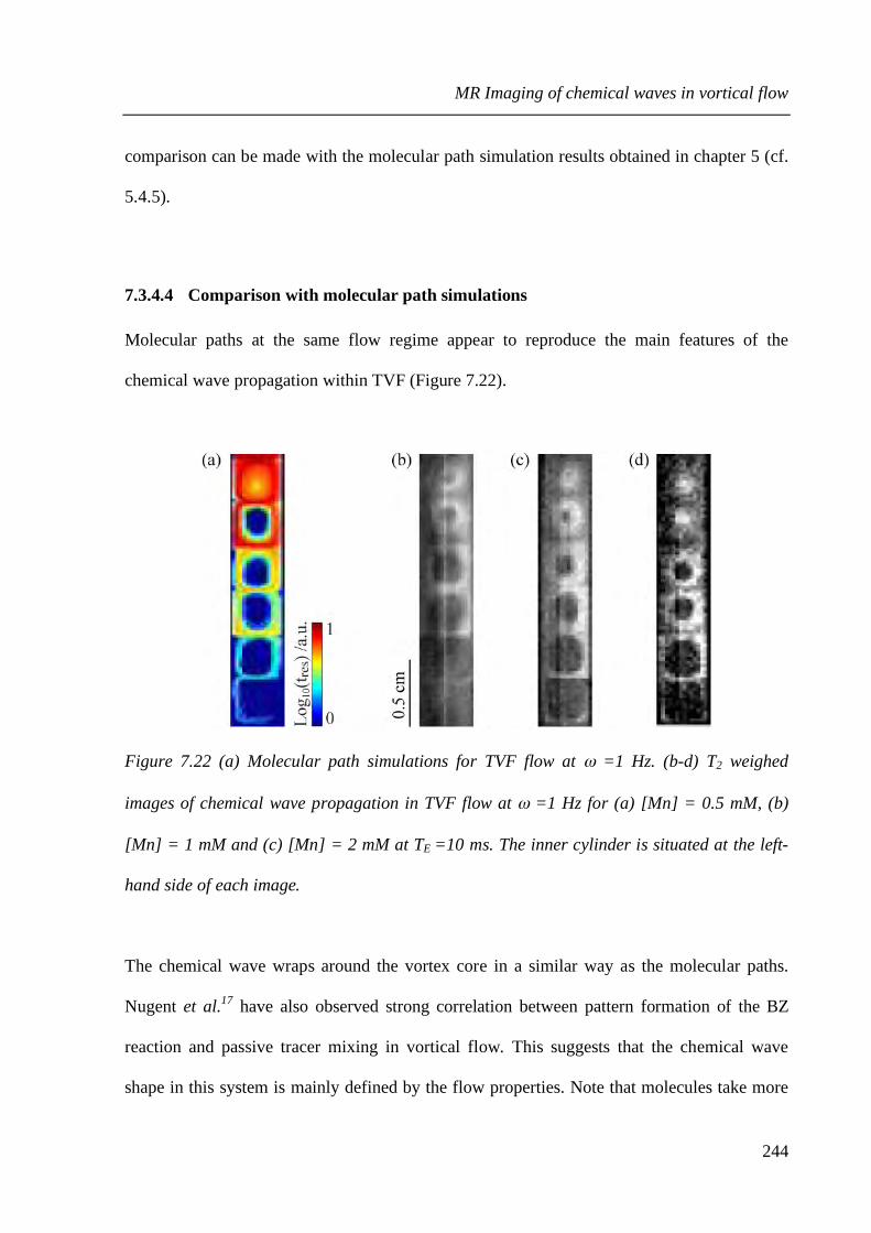
MR Imaging of chemical waves in vortical flow

244

comparison can be made with the molecular path simulation results obtained in chapter 5 (cf.

5.4.5).

7.3.4.4 Comparison with molecular path simulations

Molecular paths at the same flow regime appear to reproduce the main features of the

chemical wave propagation within TVF (Figure 7.22).

Figure 7.22 (a) Molecular path simulations for TVF flow at ω =1 Hz. (b-d) T2 weighed

images of chemical wave propagation in TVF flow at ω =1 Hz for (a) [Mn] = 0.5 mM, (b)

[Mn] = 1 mM and (c) [Mn] = 2 mM at TE =10 ms. The inner cylinder is situated at the left-

hand side of each image.

The chemical wave wraps around the vortex core in a similar way as the molecular paths.

Nugent et al.17 have also observed strong correlation between pattern formation of the BZ

reaction and passive tracer mixing in vortical flow. This suggests that the chemical wave

shape in this system is mainly defined by the flow properties. Note that molecules take more

MR Imaging of chemical waves in vortical flow

245

time to reach the vortex core in the simulation, than the time taken by the chemical wave to

consume the vortex core in the experimental results. The difference between these times could

provide with information on the relative input of flow and chemistry into the propagation of

this front. This analysis is expected to be more complicated in the case of travelling vortex

flow as the molecular paths simulations in a stationary reference frame gave very complex

outcomes.

7.3.5 MRI of travelling chemical waves in translating vortices

In the previous chapter it was shown that travelling BZ waves could be obtained in a VFR.

The waves were observed for unstable boundary conditions, when the CSTR at the inlet of the

reactor was oscillating. Similar conditions can be created if an oscillating BZ reaction mixture

is pumped in the VFR.

Figure 7.23 shows images of BZ waves (in light grey) in translating vortex flow at ω =1 Hz

and Q = 7.2 cm3 min−1. The phase oscillations of the mixture at the inlet produced waves that

travelled through the translating vortex flow until reaching the outlet of the reactor. At this

flow regime the vortices were found to travel at about 0.8 mm s−1 (Figure 7.14). Although the

wave velocity is difficult to determine with accuracy in this system, the waves appear to travel

at a similar velocity to the vortices. Also, in contrast to the results obtained for stationary

vortices, the speed of the wave is found to be similar for both Mn concentrations studied (1

mM and 2 mM). This could be due to the dominant role of flow in the wave propagation.

MR Imaging of chemical waves in vortical flow

246

Figure 7.23. Series of MR images of chemical wave propagation in travelling vortex flow at ω

=1 Hz and Q = 7.2 cm3 min−1, for (a) [Mn] = 1 mM and (b) [Mn] = 2 mM. Time interval

between the images is of 6 s. The black arrow indicates the flow direction and a schematic

representation of the vortices is given in yellow.

The analysis of the features of the propagating waves must be done with precaution as these

features present similarities with flow artifacts at the same regime (Figure 7.14). For both

manganese concentrations studied, the oxidised phase wave is seen mainly in the outer

regions of the vortices situated near the inner cylinder and in the inter-vortex areas. Note that

one over two inter-vortex areas is bended, with the outer part being lower than the inner one.

This has not been noticed in the flow artifact images. But the most surprising feature of these

images is that the vortex core and the outer part of the vortices situated near the outer cylinder

MR Imaging of chemical waves in vortical flow

247

are maintained in the reduced phase during the wave propagation. Slight phase changes in

these regions seem to affect only one vortex of each pair. This could not be attributed to flow

artifacts, as only symmetric structures were observed in flow-induced contrast images. On the

other hand, this phenomenon could be explained by the propagators obtained by molecular

displacement simulations (cf. 5.4.6) at this regime. The simulations showed both the

heterogeneous distribution of molecules into successive vortices and the bending of the inter-

vortex areas.

Figure 7.24 shows molecular path simulations in comparison with the propagating wave at

the same flow regime. The doted square in Figure 7.24a highlights molecules travelling

slower than the vortices (drag flow). Figure 7.24b is obtained by duplicating the highlighted

part of the map and changing the contrast so that regions attended by the drag flow appear in

black. Similarities can be seen between this image and the MR image of the propagating

wave. The constant arrival of molecules in the reduced state from downstream vortices

(represented in black in Figure 7.24b) could explain that the regions near the outer wall are

not reached by the chemical wave. Moreover, the regions that are not attended by the drag

flow in the simulations seem to correspond to the regions in the oxidised state on the MR

images. Both light grey regions in Figure 7.24b and the chemical waves in Figure 7.24b travel

at a similar speed to the one of the travelling vortices. On the other hand, in the simulations

only one over two inter-vortex areas is attended by drag flow molecules while the chemical

wave reaches all inter-vortex areas.

MR Imaging of chemical waves in vortical flow

248

Figure 7.24. (a) Molecular paths in the reference frame of the travelling vortices. (b) Edited

version of image (a) where regions attended by the molecules are in black colour and regions

not attended are in grey colour. (c) MR images of chemical wave propagation in travelling

vortex flow. The inner cylinder is situated at the left-hand side of each image.

As discussed earlier, precaution should be taken in interpreting these results. But even if the

simulations do not capture all the features of the propagating waves, they allow identifying

regions where the wave propagation is disturbed by the flow. These regions might correspond

to "burning invariant manifolds", BIMs. The concept of BIMs was introduced recently by

Mahoney et al.18 to describe fixed or space-periodic front propagation barriers. The existence

of such barriers, constantly maintained by the inflow of reactants, might explain the

observation of vortex areas that are not consumed by the propagating waves.

MR Imaging of chemical waves in vortical flow

249

7.3.6 MR Imaging of Mn-catalysed BZ FDOs

MR imaging was used to investigate stationary waves in translating vortex flow (FDOs). The

possibility to obtain FDOs in the VFR using the manganese-catalysed BZ reaction has been

demonstrated previously (Figure 7.4). Figure 7.25a shows images of the first stationary band

for the [Mn] = 1 mM system.

Figure 7.25. Series of MR images of the first FDO band of the [Mn] = 1 mM system at t =

2000 s. Images where taken at the centre (a) and the top (b) of the band.

The band is larger than the field of view, so only the centre of the band is seen. The vortex

cores are in the oxidised phase (light grey), while the outer areas appear to be in the reduced

phase (dark grey). As differences between phases are expected to be weak in the middle of the

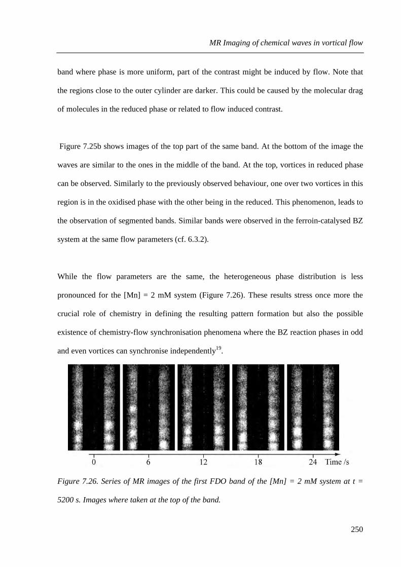
MR Imaging of chemical waves in vortical flow

250

band where phase is more uniform, part of the contrast might be induced by flow. Note that

the regions close to the outer cylinder are darker. This could be caused by the molecular drag

of molecules in the reduced phase or related to flow induced contrast.

Figure 7.25b shows images of the top part of the same band. At the bottom of the image the

waves are similar to the ones in the middle of the band. At the top, vortices in reduced phase

can be observed. Similarly to the previously observed behaviour, one over two vortices in this

region is in the oxidised phase with the other being in the reduced. This phenomenon, leads to

the observation of segmented bands. Similar bands were observed in the ferroin-catalysed BZ

system at the same flow parameters (cf. 6.3.2).

While the flow parameters are the same, the heterogeneous phase distribution is less

pronounced for the [Mn] = 2 mM system (Figure 7.26). These results stress once more the

crucial role of chemistry in defining the resulting pattern formation but also the possible

existence of chemistry-flow synchronisation phenomena where the BZ reaction phases in odd

and even vortices can synchronise independently19.

Figure 7.26. Series of MR images of the first FDO band of the [Mn] = 2 mM system at t =

5200 s. Images where taken at the top of the band.

MR Imaging of chemical waves in vortical flow

251

7.4 Conclusions

The methodology and results presented in this section set a framework for more systematic

studies that could allow getting a deeper understanding of the flow-chemistry coupling

properties of RDA systems involving vortical flow.

This work has shown that stationnary chemical waves (FDOs) can be obtained when the Mn-

catalysed BZ reaction is coupled with translating vortex flow. The wavelength of the

stationary bands was found to be not linearly dependent on the oscillation period, showing

that the chemical oscillations are not simply spatially resolved by plug-flow as suggested by

the FDO kinematic model. The catalyst concentration was shown to play an important role,

not only in defining the oscillation period of the reaction but also the wave propagation

velocity and its shape features.

For travelling waves in stationary vortices (TVF), intra-vortex consumption time was shown

to decrease with rotation, stressing the relation between intra-vortex mixing and rotation rate

in TVF. The main features of the wave propagation were shown to be similar to those of

simulated molecular paths in this flow. The possible use of this comparison in distinguishing

flow from chemistry related propagation was discussed.

For travelling chemical waves in translating vortex flow, the vortex core was maintained in

the reduced phase during the wave propagation. When stationary chemical waves were

obtained the vortex core was constantly in the oxidised phase. These features could be

explained by molecular displacements within the system or by the synchronisation between

MR Imaging of chemical waves in vortical flow

252

flow and chemistry characteristic times, where inflow and outflow of reactants in a vortex

area can maintain the reaction in a stationary state.

(1) Gao, Y.; Cross, A. R.; Armstrong, R. L. J. Phys. Chem. 1996, 100, 10159.

(2) Schlüter, A.; Weiss, A. Berichte der Bunsengesellschaft für physikalische

Chemie 1981, 85, 306

(3) Binks, D. A. Magnetic resonance studies of chemical reactions in

microemulsions, University of Birmingham, 2009.

(4) Menzinger, M.; Tzalmona, A.; Armstrong, R. L.; Cross, A.; Lemaire, C. J.

Phys. Chem. 1992, 96, 4725.

(5) Tzalmona, A.; Armstrong, R. L.; Menzinger, M.; Cross, A.; Lemaire, C. Chem.

Phys. Lett. 1990, 174, 199.

(6) Cross, A. R.; Armstrong, R. L.; Reid, A.; Su, S. Y.; Menzinger, M. J. Phys.

Chem. 1995, 99, 16616.

(7) Britton, M. M.; Sederman, A. J.; Taylor, A. F.; Scott, S. K.; Gladden, L. F. J.

Phys. Chem. A 2005, 109, 8306.

(8) Thompson, B. W.; Novak, J.; Wilson, M. C. T.; Britton, M. M.; Taylor, A. F.

Phys. Rev. E 2010, 81.

(9) Rhodes, F. H.; Barbour, C. B. Industrial and Engineering Chemistry 1923, 15,

850.

(10) Cross, A. R. The development of Three dimensional magnetic resonance

imaging of the Belousov-Zhabotisky reaction, The University of New Brunswick, 1998.

MR Imaging of chemical waves in vortical flow

253

(11) Bellon, E. M.; Haacke, E. M.; Coleman, P. E.; Sacco, D. C.; Steiger, D. A.;

Gangarosa, R. E. Am. J. Roentgenol. 1986, 147, 1271.

(12) Henkelman, R. M.; Bronskill, M. J. Med. Phys. 1987, 14, 506.

(13) Bloembergen, N.; Purcell, E. M.; Pound, R. V. Phys. Rev. 1948, 73, 679.

(14) Taylor, A. F.; Bamforth, J. R.; Bardsley, P. Phys. Chem. Chem. Phys. 2002, 4,

5640.

(15) Paoletti, M. S.; Solomon, T. H. Phys. Rev. E 2005, 72.

(16) Paoletti, M. S.; Solomon, T. H. Europhys. Lett. 2005, 69, 819.

(17) Nugent, C. R.; Quarles, W. M.; Solomon, T. H. Phys. Rev. Lett. 2004, 93.

(18) Mahoney, J.; Bargteil, D.; Kingsbury, M.; Mitchell, K.; Solomon, T. Europhys.

Lett. 2012, 98.

(19) Paoletti, M. S.; Nugent, C. R.; Solomon, T. H. Phys. Rev. Lett. 2006, 96.

Conclusions and future work

254

8 Conclusions and future work

The goal of this thesis was to develop an integrated approach to study transport and reaction

in vortical flows. This work has been carried out from two perspectives. The first consisted in

combining vortical flow with autocatalytic chemistry studies, in order to understand the

properties of the coupling between chemistry and flow within these RDA systems. The

second consisted in developing techniques and methodologies allowing systematic studies of

such RDA systems to be carried out, from the molecular to the macroscopic level.

The properties of vortical flow in a Couette cell were studied in detail. These studies provided

the first MR diffusion/dispersion maps of stationary vortex flow and the first MR velocity

maps of translating vortex flow. In the later case, it was shown that adapting the pulse

sequence to the flow period could eliminate flow artifacts caused by the periodic translation

of the vortices. This work demonstrated that the features of translating vortex flow velocity

maps could be reproduced by linear addition of pipe and stationary vortex flow velocity maps.

Propagator measurements, traditionally used in porous materials, were extended for the first

time to vortical flows. MR propagator experiments were shown to overcome the limitations of

velocity and diffusion/dispersion mapping, by addressing the complexity of molecular

displacements and micro-mixing properties of vortical flows.

Molecular displacement simulations based on experimental MR velocity and

diffusion/dispersion maps were also shown to provide rich information on the micro-mixing

properties of the flows. These simulations provided explanations both on experimental

propagator results and on molecular transport over longer time-scales, not accessible

Conclusions and future work

255

experimentally. Molecular dispersion, mixing and residence times were assessed. Also,

molecular path maps provided spatial information on molecular displacements and pathways

within the flows.

Microscopic information obtained by molecular displacement simulations, was shown to

reproduce the main features of chemical wave propagation through vortical flow. Simulated

propagators, showing heterogeneous molecular distribution within successive vortices,

provided with an explanation to the surprising phenomenon of segmented chemical waves

observed in all the autocatalytic systems considered in this thesis (bromate-sulfite clock

reaction, ferroin- and manganese-catalysed BZ reaction). These results suggest that precaution

should be taken when analysing synchronisation phenomena in systems combining

autocatalytic chemistry and vortical flow, since statistically negligible molecular

displacements might play an important role on the propagation of autocatalytic fronts. MR

imaging studies of the manganese-catalysed BZ reaction waves provided deeper insight into

the coupling between autocatalytic chemistry and vortical flow. Several features of the wave

propagation were found on the simulated molecular path maps, while their differences could

give information on the relative effects of chemistry and flow.

Macroscopic information, obtained by FDO patterns, was shown to provide information on

the mixing properties of the flow. This work showed that the combination of the BZ reaction

with travelling vortex flow produces stationary flow distributed oscillations (FDOs) for a

significant range of chemistry and flow parameters. The catalyst concentration was shown to

play an important role, not only in defining the oscillation period of the reaction, but also the

wave propagation velocity. These results emphasised the limitation of simple kinematic

Conclusions and future work

256

models in describing the macroscopic patterns resulting from the coupling of complex plug-

like flow with autocatalytic oscillatory reactions.

This thesis explored a series of techniques and methodologies that were found to produce

very promising results that would deserve further investigation. One of these techniques is the

use of MR propagators for the characterisation of mixing and the quantification of intra-and

inter-vortex mixing in vortical flow. The development of this technique could involve

systematic studies of various vortical flows at different regimes but also different PGSE

gradient axes. Another technique that deserves attention is the use of triggered pulse

sequences for the study of periodic flows. Since respiratory-triggered pulse sequences are

already commonly used in medical imaging1, the generalised use of this technique to image

periodic flows should only be a matter of time. Recently, a similar technique was used for

obtaining velocity maps of pulsatile pipe flow2. Finally, molecular displacement simulations

based on MR data was shown to provide rich information on molecular displacements within

complex systems. This method was shown to introduce quantitative analysis into RDA system

studies, which are often limited to qualitative approaches. Further refinements of the

simulations could be obtained by comparison with MR propagator data that allow a

quantitative evaluation of the simulation quality.

Although these techniques provided deeper insight into the coupling of chemistry and flow

within complex RDA systems, the results presented in this work are far from closing the list

of open questions regarding these systems. On the contrary, this work has hopefully

demonstrated the strong potential of MR techniques not only in addressing open questions,

but also in opening new questions, at levels of description that are not accessible with

Conclusions and future work

257

standard visualisation techniques. The MR techniques used in this thesis are far from

exhausting the diverse arsenal of magnetic resonance, and other MR techniques could allow

assessing complex features identified in this work. Chemical shift imaging3 could provide

with a functional imaging approach, allowing tracking the evolution of different reactants in

space. MR relaxation-resolved propagators4 could provide with insight into synchronisation

phenomena, by probing correlations between reactants and the molecular displacements. Such

propagators could be used to evaluate the quality of molecular displacement simulations

including chemical information. Ultimately, simulations of molecular displacements, taking

into account collisions that convert chemical species into each other, might quantitatively

reproduce the molecular processes that lead to the surprising macroscopic features of pattern

forming RDA systems.

(1) Kandpal, H.; Sharma, R.; Madhusudhan, K. S.; Kapoor, K. S. Am. J.

Roentgenol. 2009, 192, 915.

(2) Shiro, G.; Gladden, L. F.; Sederman, A. J.; Connolly, P. C.; Butler, J. M. J.

Pharm. Sci. 2011, 100, 976.

(3) Brateman, L. Am. J. Roentgenol. 1986, 146, 971.

(4) Britton, M. M.; Graham, R. G.; Packer, K. J. J. Magn. Res. 2004, 169, 203.

Appendix A

258

Appendix A: Imaging translating vortices in a VFR

The timed pulse sequence technique presented in chapter 4 (cf.4.2.5), successfully produced

velocity maps in a second VFR reactor. The Couette cell used in this study was constructed

from an outer glass tube of radius Ro = 8.25 mm and an inner PEEK rod of radius Ri = 5 mm,

resulting in a gap, d, of 3.25 mm. The rotation rate was of ω = 1 Hz and the flow rate of Q =

5.5 cm3 min-1. The PGSE loop time varied from TTV – 500ms to TTV + 500ms. Figure 1 shows

a series of intensity maps at different loop times and the respective velocity maps.

Figure.1. (a) Intensity maps and (b) respective velocity maps of VFR flow (ω = 1 Hz and Q =

5.5 cm3 min-1), at different PGSE sequence loop timings. The loop that eliminated the

artifacts had a period of 3.76 s.

For each one of the imaging series with increasing PGSE loop time, one single measurement

produced an intensity map with no appearing artifacts (no signal outside the gap region and

no signal loss inside the gap region). The loop time producing this intensity map corresponds

Appendix A

259

to TTV. The data acquired during this measurement was post-treated to produce a velocity map

of the measured flow. The resulting velocity map is shown in Figure 2.

Figure 2. (a) Schematic diagram of translating vortices in a VFR and (b) MR velocity map in

the z direction of VFR flow at ω = 1 Hz and Q = 5.5 cm3 min-1.

Appendix B

260

Appendix B: MATLAB code for molecular displacement

simulations

clc % clear command board

% I GENERAL PARAMETERS

% Ia Flow parameters

lamda=0.0067 % wavelength

gap=0.00475; % define the y direction distance (in m)

ttv=8.2; %(in s)

vtv=lamda/ttv; % lamda/Ttv (in m)

% Ib Calculation parameters

pclm=100 %columns of particles

prow=200 %rows of particles

vpairs=10;

realz=lamda*vpairs; %define the z direction distance as a multiple of one vortex pair wavelength (in

m)

init=lamda*3; % initial position (start third pair of vortices)

fin=lamda*7; % final position (start fourth pair of vortices)

bins=100;

dt=0.001; %time step (s)

delta=1; %mixing time (s)

% Ic Velocity/diffusion/dispersion maps parameters

yvp=13; %velocity map pixels in the y direction

Appendix B

261

y=yvp+2; %boundary zero velocity condition by adding 2 pixels atvel=0 on each side of the gap

zvprep=45; %pixels repeated in the z direction

zvi=131;

yvi=111;

gapi=44;

gapf=58;

ypix=gap/yvp; %velocity map y direction pixel dimension

zpix=realz/(vpairs*zvprep);%velocity map z direction pixel dimension

% Id Molecule tracking and analysis parameters

maxthresh=0.95;

minthresh=0.05;

mid1=0.1;

mid2=0.3;

maxorigin=zeros(y,vpairs*zvprep);

minorigin=zeros(y,vpairs*zvprep);

disorigin=zeros(y,vpairs*zvprep);

pathmap=zeros(y,vpairs*zvprep);

pathmaphalf=zeros(y,vpairs*zvprep);

pathmap0=zeros(y,vpairs*zvprep);

% II IMPORT AND ADJUST THE VELOCITY AND DIFFUSION/DISPERSION MAPS

% IIa Velocity maps

yvelmap=zeros(y,vpairs*zvprep); %define y direction experimental velocity map

zvelmap=zeros(y,vpairs*zvprep); %define z direction experimental velocity map

Appendix B

262

for v=0:(vpairs-1)

for k=1:zvprep

zvelmap(1:y,k+v*zvprep)=transpose(zdata(gapi:gapf,k+zvi));

yvelmap(1:y,k+v*zvprep)=transpose(ydata(gapi:gapf,k+yvi));

end

end

% IIb Diffusion/dispersion maps

ydiffmap=zeros(y,vpairs*zvprep); %define y direction experimental velocity map

zdiffmap=zeros(y,vpairs*zvprep); %define z direction experimental velocity map

for v=0:(vpairs-1)

for k=1:zvprep

zdiffmap(1:y,k+v*zvprep)=transpose(zdatad(gapi:gapf,k));

ydiffmap(1:y,k+v*zvprep)=transpose(ydatad(gapi:gapf,k));

end

end

%%% III GENERATE MOLECULE MATRIX

n=prow*pclm;%number of molecules followed

position0=zeros(n,2);

zstep=(fin-init)/(prow+1);

ystep=gap/(pclm+1);

x=1;

Appendix B

263

for r=0:prow

for c=0:pclm

position0(x,1)=ystep/2 + c*ystep;

position0(x,2)=init +zstep/2+ r*zstep;

x=x+1;

end

end

%%% IV MOLECULE DISPLACEMENT SIMULATION

positiont=position0;

velt=zeros(n,2);

dift=zeros(n,2);

t=0

while(t <= delta) % dt time step loop

for m=1:n

% %Wall bounceback condition

if positiont(m,1)<=0

positiont(m,1)=-positiont(m,1);

elseif positiont(m,1)>gap

positiont(m,1)=positiont(m,1)-2*(positiont(m,1)-gap);

end

%coordinates

Appendix B

264

ycoord=abs(ceil(positiont(m,1)/ypix))+1;

zcoord=abs(ceil((positiont(m,2)-vtv*t)/zpix))+1;

coefy=(positiont(m,1)/ypix)/ycoord;

%velocity

velt(m,1)=coefy*yvelmap(ycoord,zcoord)+(1-coefy)*yvelmap(ycoord-1,zcoord);

velt(m,2)=coefy*zvelmap(ycoord,zcoord)+(1-coefy)*zvelmap(ycoord-1,zcoord);

%diffusion

rnd=2*pi*rand(1);

dift(m,1)=cos(rnd)*sqrt(4*(coefy*ydiffmap(ycoord,zcoord)+(1-coefy)*ydiffmap(ycoord-

1,zcoord))*dt);

dift(m,2)=sin(rnd)* sqrt(4*(coefy*zdiffmap(ycoord,zcoord)+(1-coefy)*zdiffmap(ycoord-

1,zcoord))*dt);

pathmap(ycoord,zcoord)=pathmap(ycoord,zcoord)+1;

end

if t==dt

pathmap0=pathmap;

end

positiont(1:n,1)=positiont(1:n,1)+ dt*velt(1:n,1) + dift(1:n,1);

positiont(1:n,2)=positiont(1:n,2)+ dt*velt(1:n,2) + dift(1:n,2);

t=t+dt;

Appendix B

265

d=1;

end

%%% V DISPLACEMENTS

% Va Overall displacements

displacement=positiont(1:n,2)-position0(1:n,2);

dmax= max(displacement)

dmin=min(displacement)

% Vb Origin of max and min displacement

for m=1:n

if displacement(m)>=maxthresh*dmax

ycoord=ceil(position0(m,1)/ypix)+1;

zcoord=ceil(position0(m,2)/zpix)+1;

maxorigin(ycoord,zcoord)=maxorigin(ycoord,zcoord)+1;

elseif displacement(m)<=minthresh*dmax

ycoord=ceil(position0(m,1)/ypix)+1;

zcoord=ceil(position0(m,2)/zpix)+1;

minorigin(ycoord,zcoord)=minorigin(ycoord,zcoord)+1;

elseif (displacement(m)<=mid2*dmax)&(displacement(m)>=mid1*dmax)

ycoord=ceil(position0(m,1)/ypix)+1;

zcoord=ceil(position0(m,2)/zpix)+1;

disorigin(ycoord,zcoord)=disorigin(ycoord,zcoord)+1;

end

Appendix B

266

end

pathlog=log(pathmap);

% Vc Histogram / propagator

dstep=(dmax-dmin)/bins;

xaxis=dmin:dstep:dmax;

histo=hist(displacement,xaxis);

% for m=1:bins

% nhisto(m)=histo(m)/n

% end

plot(xaxis,histo)

title('Displacements distribution')

xlabel('displacements (m)')

ylabel('Number of particles')

Appendix C

267

Characterising stationary and translating vortex

flow using magnetic resonance Antoine Vallatos, Mark C. T. Wilson, Annette F. Taylor and Melanie M. Britton

Citation:

EPL, 99 (2012) 68001; doi: 10.1209/0295-5075/99/68001

View online:

http://iopscience.iop.org/0295-5075/99/6/68001

Appendix D

268

Chemical patterns in translating vortices: Inter- and intra-cellular

mixing effects Antoine Vallatos, Rhys Evans, Barnaby W. Thompson, Annette F. Taylor, and Melanie M.

Britton

Citation:

Chaos 23, 023115 (2013); doi: 10.1063/1.4807619

View online:

http://dx.doi.org/10.1063/1.4807619

List of Figures

269

List of Figures

Figure 1.1. Oscillations in the cerium-catalysed BZ reaction...................................................... 10

Figure 1.2. Propagation of 2D concentric waves of the BZ reaction. .......................................... 12

Figure 1.3. Similarities between the BZ reaction rotating spiral waves (left hand) and a

starving slime mold............................................................................................................ 13

Figure 1.4. Plot of the conditional probability of displacement along Z for an ensemble of

particles diffusing. ............................................................................................................. 17

Figure 1.5. (a) Exploded view of the magnetohydrodynamic forcing technique used to obtain

an annular vortex chain...................................................................................................... 19

Figure 1.6. A series of decurled images images showing the mixing of uranine dye in the

chain of vortices ................................................................................................................ 20

Figure 1.7. Convolution of the conditional probability of uniform diffusion and conditional

probability for uniform velocity. ........................................................................................ 22

Figure 1.8. Schematic diagram of a plug-flow reactor................................................................ 23

Figure 1.9. Inverse of the reaction rate against conversion for a positive order reaction in a

plug-flow reactor. .............................................................................................................. 25

Figure 1.10. Schematic diagram of a CSTR of volume V. The stirring bar ensures uniform

mixing in the reactor. ......................................................................................................... 25

Figure 1.11. Inverse of reaction rate against conversion for a positive order reaction in a single

CSTR of volume V and in a chain of four CSTRs of volumes........................................... 27

Figure 1.12. Schematic diagram of the Taylor-Couette cell mechanism. .................................... 28

Figure 1.13.Velocity maps of water TVF flow........................................................................... 30

List of Figures

270

Figure 1.14. (a) The VFR system (b) Pipe flow velocity profile and (c) Plug-flow velocity

profile................................................................................................................................ 31

Figure 1.15. Radial and axial 2D velocity vector maps in a VFR. .............................................. 34

Figure 1.16. MR images of the axisymmetric VFR flow. ........................................................... 37

Figure 1.17. Series of decurled images showing the dynamics of the BZ reaction in a vortex

chain.................................................................................................................................. 40

Figure 1.18. Experimental evidence of Turing patterns. ............................................................. 44

Figure 1.19. Schematic diagram of the Couette reactor experimental used by Ouyang et al.10.. .. 45

Figure 1.20. Patterns observed by Ouyang et al.10 at the interface between the reduced and

oxidised states of the BZ reaction in a Couette cell. ........................................................... 46

Figure 1.21.differential diffusion patterns in a pbr. .................................................................... 47

Figure 1.22. Optical images of FDOs in a PBR.......................................................................... 48

Figure 1.23. Optical images of the FDO patterns in a PBR......................................................... 49

Figure 1.24.Stationary pattern formation mechanism. ................................................................ 51

Figure 1.25. Theoretical space–time plots at low flow rate by Bamforth et al.114 and

experimental space-time plots at low flow rate by Kaern et al.115. ...................................... 52

Figure 1.26. 3D renderings of a stationary FDO band in a PBR ................................................. 54

Figure 1.27. Complex pattern development close to the critical flow rate................................... 55

Figure 1.28. Oscillatory wave propagation................................................................................. 57

Figure 2.1 precession at the Larmor frequency and schematic diagram showing the degenerate

states of 1H. ....................................................................................................................... 69

Figure 2.2. Formation of the magnetisation vector. .................................................................... 70

Figure 2.3. Schematic diagram showing a 90˚y pulse rotating the net magnetisation vector. ....... 71

Figure 2.4. The inversion recovery pulse sequence. ................................................................... 73

List of Figures

271

Figure 2.5. The a Hahn echo pulse sequence.............................................................................. 74

Figure 2.6. The CPMG pulse sequence. ..................................................................................... 75

Figure 2.7. Effect of gradients ................................................................................................... 77

Figure 2.8. Frequency encoding................................................................................................. 78

Figure 2.9. Sampling of a k-space raster ................................................................................... 79

Figure 2.10. Horizontal and vertical slice selection. ................................................................... 81

Figure 2.11. Spin echo imaging sequence. ................................................................................. 82

Figure 2.12. PGSE experiment .................................................................................................. 86

Figure 2.13. Propagators............................................................................................................ 88

Figure 2.14. PGSE and PGSTE pulse sequences. ....................................................................... 89

Figure 2.15. Pulse sequence including k-space and q-space encoding....................................... 91

Figure 3.1. Schematic diagram of the Couette cell set-up........................................................... 96

Figure 3.2. (a)–(c) MR velocity maps of TVF flow in the axial, radial and azimuthal

directions........................................................................................................................... 99

Figure 3.3. (a)–(c) MR diffusion/dispersion maps of TVF flow in the axial radial, and

azimuthal directions......................................................................................................... 101

Figure 3.4. Axial direction (z) velocity maps at increasing w. .................................................. 103

Figure 3.5. Radial direction (y) velocity maps at increasing w. ................................................ 105

Figure 3.6. Azimuthal direction (x) velocity maps at increasing w........................................... 106

Figure 3.7. Maximum velocities against rotation rate for velocity maps in the azimuthal (x),

radial (y) and axial (z) direction. ...................................................................................... 107

Figure 3.8. Vortex pair wavelength against rotation rate .......................................................... 108

Figure 3.9. Axial direction (z) diffusion/dispersion maps at increasing w................................. 109

Figure 3.10. Normalised propagators for TVF flow with w = 1 Hz at increasing mixing times. 110

List of Figures

272

Figure 3.11. Normalised propagators for TVF flow at D = 1 s for increasing rotation rates. ..... 112

Figure 3.12. Plot showing the percentage of displacements out of the region corresponding to

one vortex pair against rotation rate. ................................................................................ 113

Figure 4.1. Schematic diagram of the VFR. ............................................................................. 122

Figure 4.2. The 3 loops defining the PGSE pulse sequence had to be adapted to the period of

the translating vortices (TTV)............................................................................................ 126

Figure 4.3. Photographs of translating vortices in the VFR system........................................... 127

Figure 4.4. Plots of vortex pair wavelength against flow rate (a) and rotation rate (b). ............. 128

Figure 4.5. Plots of vortex translation velocity (a) and flow period (b) against flow rate. .......... 129

Figure 4.6. Plots of vortex translation velocity (a) and flow period (b) against rotation rate...... 130

Figure 4.7. Velocity map in the z direction of the Poiseuille flow at Q =7.2 cm3 min-1 and

Average velocity profile in the radial direction................................................................. 131

Figure 4.8. Plot showing Umax and Uax velocities of pipe flow in the Couette cell against flow

rate. ................................................................................................................................. 132

Figure 4.9 Plots of the velocity drift against flow (a) and rotation (b) rate. ............................... 133

Figure 4.10. Intensity maps of VFR flow................................................................................. 134

Figure 4.11. MR velocity maps of VFR flow in the axial, radial, and azimuthal directions....... 136

Figure 4.12. (a) Contour representation of the axial direction velocity map and 2D velocity

vector map obtained by combining the axial and radial direction velocity maps. .............. 138

Figure 4.13. MR velocity map of VFR flow obtained with an 8 q-slice PGSE experiment. ...... 139

Figure 4.14. Axial velocity map obtained by linear addition of experimental pipe flow and

TVF velocity maps .......................................................................................................... 140

Figure 4.15. Normalised average propagators for pipe flow in the z direction .......................... 144

Figure 4.16. Normalised propagators for VFR flow ................................................................. 145

List of Figures

273

Figure 4.17. Normalised average propagators for displacements in the z direction for axial, tvf

and vfr flows.................................................................................................................... 146

Figure 4.18. Normalised propagators for axial displacements in VFR flow at w= 1 Hz for

different flow rates........................................................................................................... 148

Figure 4.19. Normalised propagators for VFR flow and TVF flow for different rotation rates. 149

Figure 4.20. Normalised propagators for displacements in the z direction for VFR flow at high

flow rate .......................................................................................................................... 151

Figure 5.1. (a)–(c) Experimental propagators and (d)–(f) simulated propagators at increasing

observation times, for pipe flow at Q=7.2 cm3 min−1........................................................ 162

Figure 5.2. (a)–(c) Experimental propagators and (d)–(f) simulated propagators at increasing

observation times, for Taylor vortex flow at w =1 Hz. ..................................................... 163

Figure 5.3. (a)–(c) Experimental propagators and (d)–(f) simulated propagators at increasing

observation times, for VFR flow at w = 1 Hz and Q = 7.2 cm3 min−1. .............................. 164

Figure 5.4. Simulated propagators at D= 1 min, for pipe flow (black line) at Q =7.2 cm3 min−1

and VFR flow (red line) at w =1 Hz and Q = 7.2 cm3 min−1, with dye injection

photograph inlay.............................................................................................................. 166

Figure 5.5. Maps showing the molecular density per pixel in a simulation of molecular

displacements in pipe flow............................................................................................... 168

Figure 5.6. Velocity maps of TVF flow at w =1 Hz and maps showing the residence time (tres)

per pixel........................................................................................................................... 170

Figure 5.7. Velocity map of VFR flow and map showing the residence time (tres) per pixel...... 172

Figure 5.8. Velocity maps of VFR flow and map showing the residence time (tres) per pixel in

the reference frame of the vortices ................................................................................... 174

Figure 5.9 Upwards and downwards propagating wave front in TVF...................................... 176

List of Figures

274

Figure 5.10. Downstream front of bromocressol purple and methyl red waves in VFR flow .... 178

Figure 5.11. Upstream front of bromocressol purple and methyl red waves in VFR flow........ 180

Figure 6.1. Set-up for Pt-electrode measurements. ................................................................... 188

Figure 6.2. Experimental setup for the observation of BZ patterns in a VFR. ........................... 189

Figure 6.3. Sketch of two-zone reaction cells and processes used in the model.. ..................... 192

Figure 6.4. Temporal oscillations of the redox potential in the BZ reaction.............................. 194

Figure 6.5. schematic diagram of the VFR with translating vortices, close-up on the complete

width of the VFR for the first FDO band and complete space-time plot of FDO patterns.. 196

Figure 6.6. Space-time plots at Q = 7.2 cm3 min-1 and ω = 1 Hz .............................................. 197

Figure 6.7. Space-time plots for ω = 1 Hz at a range of flow rates............................................ 199

Figure 6.8. Close-up on the complete width of the VFR at different times for the first FDO

band of the space-time plot for Q = 10.4 cm3 min-1 and w= 1Hz. ..................................... 200

Figure 6.9. Space-time plots of a system without CSTR for ω = 1 Hz and Q = 7.2 cm3 min-1

(a) and Q = 7.2 cm3 min-1(b). .......................................................................................... 201

Figure 6.10 Space-time plots for Q = 7.2 cm3 min-1 at ω = 1.5 Hz (a) and ω = 2 Hz (b). ......... 203

Figure 6.11 Space-time plots for Q = 13.6 cm3 min-1 at a range of rotation rates. ..................... 204

Figure 6.12. (a-l) Space-time plots at a range of flow and rotation rates. .................................. 206

Figure 6.13. Phase diagram of patterns observed as function of flow and rotation rates............ 207

Figure 6.14. Plot of the average distance between stable FDO bands against flow rate for w=

1.5 Hz (---), w = 2 Hz (···) and w = 2.5 Hz (—). ............................................................... 208

Figure 6.15. Digital photographs of the second FDO band from the inlet at Q = 11.6 cm3 min–1

and for increasing rotation rate......................................................................................... 208

Figure 6.16. Phase diagram of chemical patterns with scaled flow rate (1 / Da) and scaled

inter-vortex exchange rate (1 / PeDa) when there is no intra-vortex exchange. ................. 210

List of Figures

275

Figure 6.17. Simulated space-time plots showing the critical dispersion rate for the

appearance of convective and absolute instabilities at different intra-vortex exchange

rates................................................................................................................................. 212

Figure. 6.18. Simulated space-time plots showing the effect of increasing flow rate and inter-

vortex exchange rate on the patterns at two different intra-vortex exchange rates. ............ 213

Figure 7.1. (a) Schematic diagram of the experimental set-up for phantom experiments. (b)

Transverse section of the image in (a) at the level indicated by the arrows. ...................... 224

Figure 7.2 (a) Optical contrast at increasing [Mn3+] and (b) Photoshop enhanced optical

contrast for the same picture. ........................................................................................... 227

Figure 7.3. Pt-electrode measurements of temporal oscillations in the BZ reaction for

increasing Mn concentrations........................................................................................... 229

Figure 7.4. Chemical pattern formation of the Mn-catalysed BZ reaction at w= 1 Hz and Q =

7.2 cm3 min-1 for (a) [Mn] = 0.5 mM, (b) [Mn] = 1 mM and (c) [Mn] = 2 mM................. 230

Figure 7.5 Expanded region for the first FDO band of the [Mn] = 1 mM system with enhanced

optical contrast................................................................................................................. 232

Figure 7.6 Relaxation times and relaxivities of the oxidised and reduced states of the BZ

reaction............................................................................................................................ 234

Figure 7.7 Phantom images at increasing TE for different concentrations of Mn: (a)

[Mn]=0.5mM, (a) [Mn]=1 mM and (a) [Mn]=2 mM. ..................................................... 235

Figure 7.8. Average NMR signal of the oxidised and reduced BZ states in the phantom

images for different concentrations of Mn........................................................................ 237

Figure 7.9. T2 weighed images of chemical wave propagation ([Mn]= 1 mM) in a Couette cell

without flow for different Echo and Repetition times. ...................................................... 238

List of Figures

276

Figure 7.10. T1 weighed images of tap water in a Couette cell with axial flow: (a) no flow, (b)

Q = 7.2 cm3 min-1 and Q = 13.6 cm3 min-1. ...................................................................... 239

Figure 7.11. View of the Couette cell gap from above. d represents the displacement of a

molecule on the inner cylinder surface when the cylinder rotates of θ degrees................. 240

Figure 7.12. MR images of tap water in TVF flow for different rotation rates.......................... 241

Figure 7.13. MR images of tap water in VFR flow at Q = 7.2 cm3 min-1 and for different

rotation rates. The arrow indicates the direction of the flow. ............................................ 241

Figure 7.14. Time series of MR images of tap water in VFR flow at w= 1 Hz and Q = 7.2 cm3

min-1.. .............................................................................................................................. 242

Figure 7.15. T2 relaxation time against rotation rate for tap water in a Couette cell without

flow and at Q = 7.2 cm3 min-1. ......................................................................................... 243

Figure 7.16. MR images of chemical wave propagation in TVF flow at w =1 Hz for (a) [Mn]

= 0.5 mM at TE = 20 ms, (b) [Mn] = 1 mM at TE = 15ms and (c) [Mn] = 2 mM at TE =10

ms.................................................................................................................................... 244

Figure 7.17. Series of MR images of chemical wave pacemaker in TVF flow at w =1 Hz and

for [Mn] = 1 mM. ............................................................................................................ 246

Figure 7.18. Series of MR images of chemical wave propagation in TVF flow at w =1 Hz for

(a) [Mn] = 1 mM and (b) [Mn] = 2 mM. .......................................................................... 248

Figure 7.19. Series of MR images of chemical wave propagation ([Mn] = 1 mM) in TVF flow

at w values of (a) 1.5 Hz, (b) 2 Hz and(c) 2.5 Hz. ............................................................ 249

Figure 7.20. Series of T2 weighed images of chemical wave propagation ([Mn] = 1 mM ) in

TVF flow at w values of (a) 1.5 Hz, (b) 2 Hz and(c) 2.5 Hz. ............................................ 250

Figure 7.21 Intra-vortex consumption time at different rotation rates for (a) [Mn] = 1 mM and

(b) [Mn] = 2 mM. ............................................................................................................ 251

List of Figures

277

Figure 7.22 (a) Molecular path simulations for TVF flow and T2 weighed images of chemical

wave propagation in TVF. ............................................................................................... 252

Figure 7.23. Series of MR images of chemical wave propagation in travelling vortex flow at

w =1 Hz and Q = 7.2 cm3 min-1, for (a) [Mn] = 1 mM and (b) [Mn] = 2 mM................... 254

Figure 7.24. (a) Molecular paths in the reference frame of the travelling vortices and MR

images of chemical wave propagation in travelling vortex flow ....................................... 256

Figure 7.25. Series of MR images of the first FDO band of the [Mn] = 1 mM system.............. 257

Figure 7.26. Series of MR images of the first FDO band of the [Mn] = 2 mM system.............. 259

Abbreviations

278

Abbreviations

AI: absolute instability

BZ: Belousov-Zhabotisky

CI-FDO: flow distributed oscillations formed via convective instability

CSTR: continuous stirring tank reactor

FID: free induction decay

FDO: flow distributed oscillations

FDS: flow distributed structures

FNK: Field-Noyes-Koros mechanism

NMR: nuclear magnetic resonance

NS equation: Navier-Stokes equation

MRI: magnetic resonance imaging

PBR: packed-bed reactor

PGSE: pulsed gradient spin echo

PGSTE: pulsed gradient stimulated echo

PIV: particle imaging velocimetry

RD: reaction-diffusion

RDA: reaction-diffusion-advection

rf: radio frequency

TVF: Taylor vortex flow

TW: travelling waves

VFR: vortex flow reactor