MAGNETIC FLUX LEAKAGE DATA ANALYSISFOR OIL AND GAS PIPELINE INTEGRITY

MANAGEMENT

by

Xiang Peng

B.Eng., China University of Mining and Technology, 2014

M.Sc., Beihang University, 2017

A THESIS SUBMITTED IN PARTIAL FULFILLMENTOF THE REQUIREMENTS FOR THE DEGREE OF

DOCTOR OF PHILOSOPHY

in

THE COLLEGE OF GRADUATE STUDIES(Electrical Engineering)

THE UNIVERSITY OF BRITISH COLUMBIA(Okanagan)

May 2021

© Xiang Peng, 2021

The following individuals certify that they have read, and recommend to the Col-lege of Graduate Studies for acceptance, the thesis/dissertation entitled:

MAGNETIC FLUX LEAKAGE DATA ANALYSIS FOR OIL AND GAS PIPELINEINTEGRITY MANAGEMENT

submitted by Xiang Peng in partial fulfillment of the requirements of the degreeof Doctor of Philosophy.

Dr. Zheng Liu, School of Engineering, The University of British ColumbiaSupervisor

Dr. Kasun Hewage, School of Engineering, The University of British ColumbiaSupervisory Committee Member

Dr. Hadi Mohammadi, School of Engineering, The University of British ColumbiaSupervisory Committee Member

Dr. Liwei Wang, School of Engineering, The University of British ColumbiaUniversity Examiner

Dr. Yiming Deng, College of Engineering, Michigan State UniversityExternal Examiner

ii

Abstract

Corrosion is a significant cause of oil and gas pipeline failures. In the pipelineindustry, in-line inspection (ILI) using magnetic flux leakage (MFL) technique isconducted periodically to detect and assess pipeline corrosion. The ILI data isa critical input of the pipeline integrity management (PIM) program, where thedecision on the pipeline integrity maintenance is made. This thesis research aimsto facilitate the decision-making process in the PIM program from the perspectiveof MFL data analysis.

First, the concept of parameterization is put forward to obtain a contextual rep-resentation of the corrosion defect. In the PIM program, this high-level represen-tation can help structural engineers to retrieve similar corrosion defects that couldpose serious threats to the pipeline integrity. Three parameterization models, i.e.,principal component analysis, convolutional auto-encoder, and shape context, areproposed to achieve the contextual defect representation.

Then, a computational framework is proposed to automatically match themultiple inspection results from different tools, i.e., axial MFL and circumferen-tial MFL. Due to their complementary detection capabilities, the matched multi-modal MFL data can be further integrated to obtain more comprehensive defectassessment. The proposed framework employs a sliding window searching ap-proach and a Gaussian mixture model to align the coordinate systems of two datasets. In the aligned coordinate system, an accurate matching is achieved witha modified density-based spatial clustering of applications with noise algorithm,which considers both the location and the size information of the corrosion defect.

iii

Last but not least, the detection performance of MFL inspection is assessedquantitatively. It aims to figure out which defect can be reliably detected andwhich may be missed in the MFL inspection. Therefore, even the undetecteddefects could also be considered in the PIM program. A probability of detection(POD) model is proposed to realize the quantitative performance assessment. Dueto the characteristics of MFL inspection, the proposed POD model is constructedwith two geometric variables, i.e., the volume and the orientation of a corrosiondefect. Besides, inspection results from different tools are integrated to study thePOD of their combination.

The research outcomes in this thesis contribute to the PIM program from dif-ferent perspectives. Contextual defect representation employs the MFL data fromindividual inspection to identify the pipeline integrity threat. MFL data matchingis the precondition to integrate the inspection results from different MFL toolsand eventually obtain a comprehensive corrosion defect assessment. Besides, thedetection performance assessment of MFL inspection takes the undetected defectsinto consideration and ensures no defects are ignored in the PIM program.

iv

Lay Summary

Oil and gas pipelines are subject to catastrophic failures caused by corrosion. Inthe pipeline industry, magnetic flux leakage (MFL) technique is widely employedto detect and assess pipeline corrosion. This thesis research analyzes the acquiredMFL data to help structural engineers make appropriate decisions on the pipelineintegrity maintenance.

First, a contextual representation of the corrosion defect is proposed to iden-tify the similar defects which threat the pipeline integrity. Then, a computationalframework is proposed to match inspection results from different tools, for in-stance, axial MFL and circumferential MFL. The matched data will enable furtheranalysis for a comprehensive understanding of the corrosion defect. Finally, theperformance of the MFL inspection is assessed quantitatively to ensure that eventhe undetected defects will also be considered in the maintenance.

v

Preface

This thesis is based on the research work conducted in the School of Engineeringat The University of British Columbia, Okanagan Campus, under the supervisionof Dr. Zheng Liu. I conducted the majority of the research, including the lit-erature review, problem formulation, algorithm development, and paper writing.Dr. Zheng Liu helped me with the research ideas and suggestions to improvethe quality of the manuscripts. Mr. Kevin Siggers provided his expertise in thepipeline industry which helped me to identify the research gaps. Dr. Huan Liu, Dr.Kazuhiko Tsukada, Mr. Uchenna Anyaoha, and Mr. Chengkai Zhang joined thediscussion on the research and gave their valuable feedback on the manuscripts.

Chapter 2 is based on the following published paper:

• X. Peng, U. Anyaoha, Z. Liu, and K. Tsukada, “Analysis of magnetic fluxleakage (MFL) data for pipeline corrosion assessment,” IEEE Transactions

on Magnetics, vol. 56, no. 6, pp. 1–15, Jun. 2020.

Chapter 3 is based on the following published papers:

• X. Peng, H. Liu, K. Siggers, and Z. Liu, “Pipeline corrosion defect param-eterization with magnetic flux leakage inspection: a contextual representa-tion approach,” Insight - Non-Destructive Testing & Condition Monitoring,vol. 63, no. 2, pp. 95–101, Feb. 2021.

• X. Peng, C. Zhang, U. Anyaoha, K. Siggers, and Z. Liu, “Parameterizingmagnetic flux leakage data for pipeline corrosion defect retrieval,” in 2019

vi

IEEE 28th International Symposium on Industrial Electronics (ISIE), pp.2665-2670, Jun. 2019 (IEEE IES Young Professionals & Student Paper

Assistance Award).

Chapter 4 is based on the following published papers:

• X. Peng, H. Liu, K. Siggers, and Z. Liu, “Automated box data matching formulti-modal magnetic flux leakage inspection of pipelines,” IEEE Transac-

tions on Magnetics, vol. 57, no. 5, pp. 1–10, May 2021.

• X. Peng, K. Siggers, and Z. Liu, “Multi-MFL measurement assessmentusing Gaussian mixture model,” in 2019 3rd International Conference on

Sensing, Diagnostics, Prognostics, and Control (SDPC), pp. 529-534, Aug.2019.

Chapter 5 is based on the following submitted paper:

• X. Peng, K. Siggers, and Z. Liu, “Performance assessment of multi-MFLinspection using feature-based POD,” Insight - Non-Destructive Testing &

Condition Monitoring (Under Review).

Other publications I co-authored are summarized as follows:

• F. Shi, X. Peng, Z. Liu, E. Li, and Y. Hu, “A data-driven approach for pipedeformation prediction based on soil properties and weather conditions,”Sustainable Cities and Society, vol. 55, p. 102012, Apr. 2020.

• S. Liu, X. Peng, and Z. Liu, “Image quality assessment through contourdetection,” in 2019 IEEE 28th International Symposium on Industrial Elec-

tronics (ISIE), pp. 1413-1417, Jun. 2019.

• U. Anyaoha, X. Peng, H. Liu, Y. Hu, Z. Liu, and E. Li, “Concrete perfor-mance prediction using boosting smooth transition regression trees (BooST),”in Nondestructive Characterization and Monitoring of Advanced Materials,

Aerospace, Civil Infrastructure, and Transportation XIII, p. 109710I, Apr.2019.

vii

• F. Shi, X. Peng, H. Liu, Y. Hu, Z. Liu, and E. Li, “Soil-pipe interactionmodeling for pipe behavior prediction with super learning based methods,”in Smart Structures and NDE for Industry 4.0, p. 1060207, Mar. 2018.

viii

Table of Contents

Abstract . . . . . . . . . . . . . . . . . . . . . . . . . . . . . . . . . . . . iii

Lay Summary . . . . . . . . . . . . . . . . . . . . . . . . . . . . . . . . v

Preface . . . . . . . . . . . . . . . . . . . . . . . . . . . . . . . . . . . . vi

Table of Contents . . . . . . . . . . . . . . . . . . . . . . . . . . . . . . ix

List of Tables . . . . . . . . . . . . . . . . . . . . . . . . . . . . . . . . . xii

List of Figures . . . . . . . . . . . . . . . . . . . . . . . . . . . . . . . . xiii

Glossary . . . . . . . . . . . . . . . . . . . . . . . . . . . . . . . . . . . xvi

Acknowledgments . . . . . . . . . . . . . . . . . . . . . . . . . . . . . . xviii

1 Introduction . . . . . . . . . . . . . . . . . . . . . . . . . . . . . . . 11.1 Background and Motivations . . . . . . . . . . . . . . . . . . . . 1

1.1.1 Pipeline Integrity Management . . . . . . . . . . . . . . . 21.1.2 Magnetic Flux Leakage Technique . . . . . . . . . . . . . 7

1.2 Related Work . . . . . . . . . . . . . . . . . . . . . . . . . . . . 131.2.1 Contextual Corrosion Defect Representation . . . . . . . . 131.2.2 MFL Data Matching . . . . . . . . . . . . . . . . . . . . 151.2.3 Probability of Detection . . . . . . . . . . . . . . . . . . 17

ix

1.2.4 Research Gaps . . . . . . . . . . . . . . . . . . . . . . . 181.3 Research Objectives . . . . . . . . . . . . . . . . . . . . . . . . . 191.4 Thesis Outline . . . . . . . . . . . . . . . . . . . . . . . . . . . . 20

2 Magnetic Flux Leakage Technique for Pipeline Corrosion Assessment 232.1 Overview . . . . . . . . . . . . . . . . . . . . . . . . . . . . . . 232.2 Corrosion Quantification with Individual MFL Inspection . . . . . 25

2.2.1 MFL Signal Denoising . . . . . . . . . . . . . . . . . . . 252.2.2 Corrosion Defect Characterization . . . . . . . . . . . . . 30

2.3 Corrosion Growth Prediction with Multiple MFL Inspections . . . 382.3.1 Deterministic Corrosion Growth Models . . . . . . . . . . 392.3.2 Probabilistic Corrosion Growth Models . . . . . . . . . . 40

2.4 Computational Models for Pipeline Reliability Analysis . . . . . . 442.5 Fusion of MFL and Other NDT Data . . . . . . . . . . . . . . . . 462.6 Summary . . . . . . . . . . . . . . . . . . . . . . . . . . . . . . 48

3 Contextual Defect Representation with Magnetic Flux Leakage Data 493.1 Overview . . . . . . . . . . . . . . . . . . . . . . . . . . . . . . 503.2 Implementation of Corrosion Defect Parameterization Models . . 53

3.2.1 Principal Component Analysis based Model . . . . . . . . 533.2.2 Convolutional Auto-Encoder based Model . . . . . . . . . 543.2.3 Shape Context based Model . . . . . . . . . . . . . . . . 563.2.4 Interaction Strength Function . . . . . . . . . . . . . . . . 57

3.3 Experimental Results and Discussions . . . . . . . . . . . . . . . 573.3.1 Experimental Setup . . . . . . . . . . . . . . . . . . . . . 573.3.2 Similar Corrosion Defect Retrieval . . . . . . . . . . . . . 583.3.3 Corrosion Defect Population Analysis . . . . . . . . . . . 63

3.4 Summary . . . . . . . . . . . . . . . . . . . . . . . . . . . . . . 65

4 Automated Box Data Matching for Multi-Modal Magnetic Flux Leak-age Inspections . . . . . . . . . . . . . . . . . . . . . . . . . . . . . . 66

x

4.1 Overview . . . . . . . . . . . . . . . . . . . . . . . . . . . . . . 674.2 Implementation of Automated Data Matching Framework . . . . . 69

4.2.1 Data Pre-Processing: Mapping and Cleansing . . . . . . . 714.2.2 Grouping the CMFL Box Data . . . . . . . . . . . . . . . 724.2.3 Aligning the Coordinate Systems . . . . . . . . . . . . . . 754.2.4 Matching Box Data in the Aligned Coordinate System . . 78

4.3 Experimental Results and Discussions . . . . . . . . . . . . . . . 794.3.1 Experimental Setup . . . . . . . . . . . . . . . . . . . . . 794.3.2 Matching Results with Different Radii . . . . . . . . . . . 804.3.3 Comparative Study . . . . . . . . . . . . . . . . . . . . . 82

4.4 Summary . . . . . . . . . . . . . . . . . . . . . . . . . . . . . . 85

5 Performance Assessment of Multi-Modal MFL Inspections usingFeature-based POD . . . . . . . . . . . . . . . . . . . . . . . . . . . 865.1 Overview . . . . . . . . . . . . . . . . . . . . . . . . . . . . . . 865.2 Probability of Detection Model . . . . . . . . . . . . . . . . . . . 88

5.2.1 Selection of Defect Variables . . . . . . . . . . . . . . . . 885.2.2 POD Combination of Multiple MFL Inspections . . . . . . 90

5.3 Experimental Results and Discussions . . . . . . . . . . . . . . . 915.3.1 Experimental Setup . . . . . . . . . . . . . . . . . . . . . 915.3.2 Probability of Detection Surface . . . . . . . . . . . . . . 91

5.4 Summary . . . . . . . . . . . . . . . . . . . . . . . . . . . . . . 95

6 Conclusions . . . . . . . . . . . . . . . . . . . . . . . . . . . . . . . . 966.1 Contributions . . . . . . . . . . . . . . . . . . . . . . . . . . . . 976.2 Limitations and Future Work . . . . . . . . . . . . . . . . . . . . 98

Bibliography . . . . . . . . . . . . . . . . . . . . . . . . . . . . . . . . . 100

xi

List of Tables

Table 1.1 Comparison between three main in-line inspection (ILI) tech-niques. . . . . . . . . . . . . . . . . . . . . . . . . . . . . . . 6

Table 2.1 Summary of the measurement variations and corresponding sig-nal processing methods. . . . . . . . . . . . . . . . . . . . . . 30

Table 2.2 Comparison between dipole model and finite element model. . 33Table 2.3 Summary of corrosion defect growth models. . . . . . . . . . . 45Table 2.4 Fusion of MFL and other NDT data. . . . . . . . . . . . . . . 47

Table 3.1 Description of corrosion defect variables. . . . . . . . . . . . . 50Table 3.2 Comparison between all parameterization models associated

with the interaction strength function (ISF). . . . . . . . . . . . 61

Table 4.1 Details on the selected six pipe joints. . . . . . . . . . . . . . . 79Table 4.2 Comparison between different matching schemes. . . . . . . . 83

xii

List of Figures

Figure 1.1 Oil and gas pipeline system in Canada (Photo courtesy of OilSands Magazine) [1]. . . . . . . . . . . . . . . . . . . . . . . 2

Figure 1.2 Pipeline incidents categorized by causes. . . . . . . . . . . . . 3Figure 1.3 Framework of the pipeline integrity management (PIM) pro-

gram. . . . . . . . . . . . . . . . . . . . . . . . . . . . . . . 4Figure 1.4 A pipeline inspection gauge (PIG) tool running inside pipeline

(Photo courtesy of Intertek Group) [2]. . . . . . . . . . . . . . 6Figure 1.5 Two typical types of MFL inspection tools (Photo courtesy of

ROSEN Group) [3]. . . . . . . . . . . . . . . . . . . . . . . . 8Figure 1.6 An example of pipeline corrosion and the corresponding MFL

signals. Units mm and mT denote millimeter and millitesla,respectively. . . . . . . . . . . . . . . . . . . . . . . . . . . . 9

Figure 1.7 Pipeline corrosion detection with the magnetic flux leakage(MFL) technique. . . . . . . . . . . . . . . . . . . . . . . . . 10

Figure 1.8 An example of AMFL data from a pipe joint. Unit mT denotesmillitesla, and % denotes the percent of corrosion depth. . . . 11

Figure 1.9 An example of CMFL data from a pipe joint. Unit mT denotesmillitesla, and % denotes the percent of corrosion depth. . . . 12

Figure 1.10 Outline of this thesis. . . . . . . . . . . . . . . . . . . . . . . 21

Figure 2.1 Corrosion quantification with individual MFL inspection. . . . 24Figure 2.2 Corrosion prediction with multiple MFL inspections. . . . . . 24

xiii

Figure 2.3 Illustration of the forward and the inverse processes of corro-sion defect characterization. . . . . . . . . . . . . . . . . . . 31

Figure 2.4 Flowchart of iterative inverse defect profiling model. . . . . . 34Figure 2.5 Reliability analysis of corroded pipeline. . . . . . . . . . . . . 44

Figure 3.1 Graphical illustration of corrosion defect variables. . . . . . . 51Figure 3.2 Corrosion defect parameterization and its applications. . . . . 52Figure 3.3 Structure of the convolutional auto-encoder based model. . . . 55Figure 3.4 Feature extraction in the shape context based model. The cor-

rosion area is first divided into sections, then the informationof the defects locating in each section are collected. . . . . . . 56

Figure 3.5 Manually selected corrosion defects. The sample dimensionis 200mm× 200mm, and % denotes the percent of corrosiondepth. . . . . . . . . . . . . . . . . . . . . . . . . . . . . . . 59

Figure 3.6 Query corrosion defect (The sample dimension is 200mm×200mm, and % denotes the percent of corrosion depth). . . . . 61

Figure 3.7 Histogram of the similarity between the query and the wholedata set. . . . . . . . . . . . . . . . . . . . . . . . . . . . . . 62

Figure 3.8 Top four retrieval corrosion defects. The sample dimension is200mm×200mm, and % denotes the percent of corrosion depth. 62

Figure 3.9 T-SNE plots from three parameterization models. . . . . . . . 64Figure 3.10 Corrosion defect samples from the t-SNE plot. The sample

dimension is 200mm×200mm, and % denotes the percent ofcorrosion depth. . . . . . . . . . . . . . . . . . . . . . . . . . 65

Figure 4.1 Pipeline corrosion inspection with multi-modal MFL data. Thischapter focuses on the step of box data matching, which ishighlighted with the dashed rectangle. . . . . . . . . . . . . . 67

Figure 4.2 Proposed multi-modal MFL data matching framework, whichincludes data pre-processing, grouping, alignment, and match-ing. . . . . . . . . . . . . . . . . . . . . . . . . . . . . . . . 70

xiv

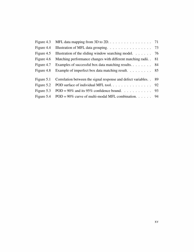
Figure 4.3 MFL data mapping from 3D to 2D. . . . . . . . . . . . . . . . 71Figure 4.4 Illustration of MFL data grouping. . . . . . . . . . . . . . . . 73Figure 4.5 Illustration of the sliding window searching model. . . . . . . 76Figure 4.6 Matching performance changes with different matching radii. . 81Figure 4.7 Examples of successful box data matching results. . . . . . . . 84Figure 4.8 Example of imperfect box data matching result. . . . . . . . . 85

Figure 5.1 Correlation between the signal response and defect variables. . 89Figure 5.2 POD surface of individual MFL tool. . . . . . . . . . . . . . . 92Figure 5.3 POD = 90% and its 95% confidence bound. . . . . . . . . . . 93Figure 5.4 POD = 90% curve of multi-modal MFL combination. . . . . . 94

xv

Glossary

AMFL Axial Magnetic Flux Leakage

CAE Convolutional Auto-Encoder

CMFL Circumferential Magnetic Flux Leakage

CNN Convolution Neural Network

DBSCAN Density-Based Spatial Clustering of Applications with Noise

DM Dipole Model

EC Eddy Current

ELM Extreme Learning Machine

EM Expectation Maximization

FCN Fully Convolutional Network

FEM Finite Element Method

FIR Finite Impulse Response

GMM Gaussian Mixture Model

HOST Higher Order Statistics Transformation

ILI In-Line Inspection

xvi

ISF Interaction Strength Function

MCMC Markov Chain Monte Carlo

MFL Magnetic Flux Leakage

NDCG Normalized Discounted Cumulative Gain

NDT Non-Destructive Testing

PCA Principal Component Analysis

PCC Pearson’s Correlation Coefficient

PIG Pipeline Inspection Gauge

PIM Pipeline Integrity Management

POD Probability of Detection

POF Pipeline Operator Forum

RBFNN Radial Basis Function Neural Network

RPM Robust Point Matching

RUL Remaining Useful Life

SC Shape Context

SWS Sliding Window Searching

SVD Singular Value Decomposition

T-SNE T-Distributed Stochastic Neighbor Embedding

UT Ultrasound Testing

xvii

Acknowledgments

I would like to take this opportunity to thank those who supported and helped meto complete my Ph.D. journey.

I owe my deepest gratitude to my supervisor Dr. Zheng Liu for his constantguidance and encouragement. His great enthusiasm and passion for research in-spired me to move forward. He taught me to be logical and enthusiastic about theresearch. It was a great honor for me to work under his supervision.

I am also grateful to Dr. Kasun Hewage and Dr. Hadi Mohammadi to be onmy supervisory committee. I would like to thank Dr. Liwei Wang to serve asthe university examiner. I want to thank Dr. Yiming Deng from Michigan StateUniversity for his willingness to serve as my external examiner. I appreciate theirvaluable suggestions and critical comments on my research and thesis.

I would like to thank my colleagues at the Intelligent Sensing, Diagnostics andPrognostics Research Lab (ISDPRL). Thanks for their help on both research andeveryday life. Their company makes this journey even more memorable.

ROSEN Canada Ltd. and NSERC are acknowledged for their financial supportthrough the “Collaborative Research and Development Grants” (CRDPJ515074-17). Especially, I would like to thank Mr. Kevin Siggers from ROSEN CanadaLtd. for sharing his expertise in the pipeline industry.

Finally, I want to present my greatest gratitude to my beloved family. None ofmy dreams could be achieved without their unconditional love and support.

xviii

Chapter 1

Introduction

1.1 Background and MotivationsThe pipeline is the primary option to transport and distribute large quantities ofoil and gas products over a long distance because of its safety, large transmissioncapacity, and low cost [4, 5]. There are over 840,000km of oil and gas pipelinesacross Canada as shown in Fig. 1.1. In 2014, federally regulated pipelines shippedabout 159 billion dollars worth of oil and gas product to domestic and internationalcustomers at an estimated transportation cost of 7 billion dollars [6].

However, pipeline failures, e.g., leakage or ruptures, could lead to enormousdamage to properties, environment, and even human lives [7]. Data from thePipeline and Hazardous Materials Safety Administration indicate that all reported11,751 pipeline incidents, in the past twenty years, cost 1,292 human lives andmore than 7.2 billion dollars [8].

Research shows corrosion is one of the significant causes for pipeline fail-ures [9, 10]. As shown in Fig. 1.2, about 18% of pipeline incidents are caused bycorrosion, only second to excavation damage [11, 12]. Corrosion is an electro-chemical deterioration process that happens when the metal pipeline is exposedto the corrosive environment [13, 14]. Corrosion can result in metal loss on thepipeline surface which reduces the wall thickness of the pipe and causes the pipe

1

Figure 1.1: Oil and gas pipeline system in Canada (Photo courtesy of OilSands Magazine) [1].

to lose its strength [15]. Without intervention, the metal loss from corrosioncan eventually result in pipeline leakage or ruptures. Because of the severity ofpipeline failures, it is critical to keep the pipeline operating under the safe condi-tion.

1.1.1 Pipeline Integrity ManagementTo manage the integrity of the pipeline system and make it suitable for continuedservice, operating companies are required to develop and implement a pipelineintegrity management (PIM) program [16–18]. The PIM is a preventative frame-work that specifies the processes and practices to analyze, assess, and managepipeline risks [19, 20]. The core processes of PIM are illustrated with Fig. 1.3 andcan be broken down into four aspects, i.e., PLAN, DO, CHECK, and ACT [21].

In step PLAN, the integrity maintenance plan is developed considering allavailable information, including safety policies, pipe properties, operational char-acteristics, historical maintenance records, and previous inspection results. Thepipeline integrity is first assessed and then the plan for monitoring and mitigation

2

Figure 1.2: Pipeline incidents categorized by causes.

operations is made.For a given pipe segment, its integrity condition is quantified in terms of the

defect density, severity, and growth rate. This quantified condition is the founda-tion to develop the maintenance plan for the pipe segment. The plan may includethe timing and approach for the defect inspection, pipeline operation pressure re-duction, cathodic protection, recoating, and pipe segment replacement [22]. Thereare two objectives to achieve by this plan. One objective is to minimize the main-tenance cost with the acceptance of certain risk level. The other objective is tominimize the risk, mainly aiming to reduce the probability of failure and/or theseverity of failure [23].

In step DO, the planned maintenance operations are conducted in order tokeep the safety of the pipeline operation. The pipe segments with identified de-fects will be excavated, and corresponding mitigation operations including re-coating and replacement will be conducted based on the severity of the defect.For the pipe segments exposed to the corrosive environment, cathodic protection

3

Figure 1.3: Framework of the pipeline integrity management (PIM) program.

4

technique will be introduced to slow down the corrosion progress [24–26]. Allconducted maintenance operation will be recorded for the next round of pipelineintegrity management.

The step CHECK evaluates the effectiveness of the conducted maintenanceoperations by comparing against expected results. This step takes the pipelineproperties, inspection accuracy, operating condition, and maintenance record asinputs to predict the probability of failure after the maintenance operations. Thesafety requirement must be satisfied before it goes to the PLAN step, otherwise, itgoes to step ACT for addition actions.

The step ACT will only be considered when the conducted maintenance oper-ations does not achieve the expected goals. It means the current integrity programneeds to be further improved. In this step, the pipeline operation pressure will bereduced to ensure the pipeline safety. Then, additional inspection result analysisand data calibration will be conducted to identify the root issues. Then the corre-sponding operations will be employed to maintain the pipeline integrity. And theintegrity program will be modified for the future use.

The effectiveness of pipeline integrity management (PIM) program highly re-lies on the quality of the available data of certain pipelines. Precise data givestructural engineers an accurate assessment on the pipeline integrity and thereforeproper maintenance plan can be developed. Within all the data in PIM, in-line in-spection (ILI) data provides the highest quality information to achieve an effectiveintegrity management program [21].

ILI is a common practice used to assess the integrity of oil and gas pipelinesfrom the inside of the pipe [27, 28]. ILI involves the use of advanced tools, whichare known as pipeline inspection gauge (PIG). An example of PIG tool is shownin Fig 1.4. PIG is deployed inside the pipeline and utilize non-destructive testing(NDT) to identify pipeline corrosion.

The commonly used ILI techniques include eddy current (EC), ultrasound test-ing (UT), and magnetic flux leakage (MFL). The advantages and limitations ofthem are summarized in Table. 1.1. Compared with other ILI techniques, MFL

5

Figure 1.4: A pipeline inspection gauge (PIG) tool running inside pipeline(Photo courtesy of Intertek Group) [2].

Table 1.1: Comparison between three main in-line inspection (ILI) tech-niques.

ILI techniques Advantages Limitations

Eddy current(EC)

Good at sizing the smalldefect.

Cannot detect the external de-fect.

Ultrasoundtesting (UT)

Directly measures the wallthickness.

Only applicable to oilpipeline;Requires clean line condition.

Magneticflux leakage(MFL)

Applicable to both oil andgas pipeline;Good at detecting both in-ternal and external defect.

Cannot directly measure thewall thickness.

has the following advantages: 1) it can detect both internal and external defects;2) it is applicable in both liquid and gas medium; 3) it is more efficient [29, 30].These advantages make MFL become the most common ILI technique to detectand quantify the corrosion defect in oil and gas pipelines.

6

1.1.2 Magnetic Flux Leakage TechniqueThe phenomenon of magnetic flux leakage (MFL) was first found by Hoke in1918 [31]. From the 1960s, MFL technique starts being adopted in intelligentpipeline inspection gauge (PIG) tools to detect metal loss in oil and gas pipeline.Nowadays, it has become the most common in-line inspection (ILI) technique forpipeline corrosion detection.

As the MFL tool runs inside the pipeline, its strong magnets generate a saturat-ing magnetic field into the pipe wall until no more magnetic flux can be held [32].If the pipe wall is intact, all magnetic flux will keep inside the pipe wall since it iseasier to magnetize [33, 34], and the magnetic field is distributed uniformly [35].Otherwise, when corrosion defects exist on the pipe wall, the wall thickness willdecrease and therefore it cannot hold the original flux density. Part of the fluxwill leak out of the pipe wall and into the air. The flux leakage is measured bythe Hall sensors which are built in the MFL tool and recorded in the on-boardmemory [36]. The distribution and amount of flux leakage depend on the de-fect geometry. Therefore, the corrosion defect can be estimated by analyzing thecollected MFL signal.

The measurement capability of the MFL tool is highly related to the directionof its magnetic field [37, 38]. It is only sensitive to the defect component whichis orthogonal to its magnetic field [35]. The magnetic field of the conventionalMFL is along the axial direction of the pipeline. Therefore, the conventional MFLis also known as AMFL. The typical image, setup, and detection characteristicsof AMFL tool are presented in Fig. 1.5a, Fig. 1.5b, and Fig. 1.5c [3]. This typeof MFL tool is poor at detecting axially oriented features which are parallel withits magnetic field. To address this problem, circumferential MFL (CMFL) withcircumferential magnetic field is developed [39]. The typical image, setup, anddetection characteristics of CMFL tool are presented in Fig. 1.5d, Fig. 1.5e, andFig. 1.5f. Besides AMFL and CMFL, a third MFL tool with spiral magnetic fieldis proposed in [40, 41]. However, this type of MFL tool is not included in thisthesis research because the information on it is limited in the published literature.

7

(a) Image of the AMFL tool.

SNSensor

Magnet

Corrosion defect

Pipe

(b) Setup of the AMFL. (c) Characteristics of the AMFL.

(d) Image of the CMFL tool.

Sensor

Corrosion defect

Magnet

Pipe

(e) Setup of the CMFL. (f) Characteristics of the CMFL.

Figure 1.5: Two typical types of MFL inspection tools (Photo courtesy of ROSEN Group) [3].

8

0 100 200 300 400 500 600 700Axial distance (mm)

0

100

200

300Circum

ferential d

istan

ce (mm)

0.0

0.5

1.0

1.5

2.0

2.5mm

(a) Laser scan showing the corrosion depth.

0 100 200 300 400 500 600 700Axial distance (mm)

0

100

200

300

Circum

ferential d

istan

ce (m

m)

0.0

2.5

5.0

7.5

10.0mT

(b) Corresponding AMFL signals.

0 100 200 300 400 500 600 700Axial distance (mm)

0

100

200

300

Circum

ferential d

istan

ce (m

m)

0

10

20

mT

(c) Corresponding CMFL signals.

Figure 1.6: An example of pipeline corrosion and the corresponding MFLsignals. Units mm and mT denote millimeter and millitesla, respec-tively.

9

To further illustrate the detection characteristics of AMFL and CMFL inspec-tion tools, an example of pipeline corrosion and the corresponding MFL signalsare given in Fig. 1.6. The corrosion depth of this area is measured with laser scanand shown in Fig. 1.6a. The AMFL signals in Fig. 1.6b have a significant re-sponse on the bottom circumferential defect but rather weak response on the topaxial defect even though it is much deeper. On the other hand, the CMFL signalsin Fig. 1.6c are very responsive to the axial defect. To sum up, AMFL is good atdetecting circumferential defects while CMFL is more accurate at sizing axiallyoriented features[40, 41]. Because of their complementary detection capabilities,two types of MFL tools are usually employed in the inspection to capture moreinformation of the corrosion defect.

Decision makingMaintenance

MFL tool MFL signal Sizing model MFL boxPipeline

PIM database

Figure 1.7: Pipeline corrosion detection with the magnetic flux leakage(MFL) technique.

The general procedure for pipeline corrosion detection with MFL techniquecan be illustrated with Fig. 1.7. First, the MFL tool is sent to run inside thepipeline and collect the MFL signal as shown in Fig. 1.8a and Fig. 1.9a. Thesignal data only give the strength of the MFL signal response, and it is a challengefor structural engineers to directly understand and interpret them. Therefore, theacquired signals will be fed into the sizing model to quantify the corrosion defect.The output of the sizing model, also known as box data as shown in Fig. 1.8b

10

0 500 1000 1500 2000 2500 3000 3500 4000Axial distance (mm)

0

200

400

600

800

Circum

ferential d

istan

ce (m

m)

−1

0

1

2

3

4

mT

(a) AMFL signal data.

0 500 1000 1500 2000 2500 3000 3500 4000Axial distance (mm)

0

200

400

600

800

Circum

ferential d

istan

ce (mm)

0

10

20

30

40%

(b) AMFL box data.

Figure 1.8: An example of AMFL data from a pipe joint. Unit mT denotes millitesla, and % denotes thepercent of corrosion depth.

11

0 500 1000 1500 2000 2500 3000 3500 4000Axial distance (mm)

0

200

400

600

800

Circum

ferential d

istan

ce (m

m)

0

10

20

30mT

(a) CMFL signal data.

0 500 1000 1500 2000 2500 3000 3500 4000Axial distance (mm)

0

200

400

600

800

Circum

ferential d

istan

ce (mm)

0

10

20

30

40%

(b) CMFL box data.

Figure 1.9: An example of CMFL data from a pipe joint. Unit mT denotes millitesla, and % denotes thepercent of corrosion depth.

12

and Fig. 1.9b, gives the length, width, and depth of the defect. The inspectionresults, box data, will be presented to structural engineers along with other dataon this pipeline in the PIM database. Based on this information, the decisionon the maintenance operation will be made. The pipe joints which are corrodedseriously will be excavated for coating or replacement operation.

Current pipeline inspection using MFL technique has several limitations. First,the MFL inspection results, box data, only give the profile of individual corrosiondefect. However, the structural safety of a pipeline not only depends on the pro-file of individual corrosion defect but also the pattern of closely spaced defects.Then, the inspection results from different MFL tools are presented to the struc-tural engineers separately. The defect assessment from individual MFL tool couldbe unreliable due to its limited detection capability. Besides, certain corrosiondefects could be missed in the inspection because of the characteristics of MFLtechnique. The undetected defects are ignored in the PIM program and could leadto pipeline failures.

1.2 Related WorkIn order to find the potential solutions to the limitations of the current pipelineinspection, this section gives a comprehensive review on the related research,including contextual corrosion defect representation, magnetic flux leakage datamatching, and probability of detection.

1.2.1 Contextual Corrosion Defect RepresentationIn this research, the concept of contextual corrosion defect representation is putforward. It is the process to obtain a fixed length vector which can contextu-ally represent the corrosion defect. It is similar with the image feature in contentbased image retrieval problem. Therefore, the state-of-the-art of image featuresis reviewed. In a broad sense, image features may include both text based fea-tures (key words, annotations), visual features (color, texture, shape) and features

13

extracted from convolution neural network (CNN). Since no text information ex-ists for the MFL data, only visual features and CNN features are covered in thefollowing.

The color feature is one of the most widely used visual features in imageretrieval. It is relatively robust to background complication and independent ofimage size and orientation. Some representative studies of color perception andcolor spaces can be found in [42, 43]. In image retrieval, the color histogram isthe most commonly used color feature representation. Statistically, it denotes thejoint probability of the intensities of the three color channels. Besides the colorhistogram, several other color feature representations have been applied in imageretrieval, including color moments and color sets [44].

Texture refers to the visual patterns that have properties of homogeneity thatdo not result from the presence of only a single color or intensity [45]. It isan innate property of virtually all surfaces, including clouds, trees, bricks, hair,and fabric. It contains important information about the structural arrangement ofsurfaces and their relationship to the surrounding environment [46]. Because ofits importance and usefulness in pattern recognition and computer vision, thereare rich research results from the past three decades. Now, it further finds its wayinto image retrieval. More and more research achievements are being added to it.

In general, the shape representations can be divided into two categories, bound-ary based and region based. The former uses only the outer boundary of the shapewhile the latter uses the entire shape region [47]. The most successful representa-tives for these two categories are Fourier descriptor and moment invariants. Themain idea of a Fourier descriptor is to use the Fourier transformed boundary asthe shape feature. Some early work can be found in [48, 49]. The main idea ofmoment invariants is to use region based moments which are invariant to transfor-mations, as the shape feature. In [50], Hu identified seven such moments. Basedon his work, many improved versions has emerged [51, 52].

In recent years, convolutional neural network (CNN) has become a hot topicand has achieved very good results in image classification, retrieval, detection and

14

other related fields. Compared with conventional methods using domain expertknowledge, CNN requires only a set of training data that allows to discover thefeature extraction in a self-taught manner [53, 54].

The general framework of convolutional neural network can be illustrated asfollowing. The input images with fixed size are convolved with multiple learnedkernels using shared weights. Then, the pooling layers down-sample the in-put representation non-linearly and preserve the feature information in each sub-region. Afterwards, the extracted features are weighted and combined in the fully-connected layer, and these features are sent to a pre-defined classifier for predic-tion. Finally, by comparing the output class with the image label, the CNN pa-rameters are updated in each iteration. Experimental results have shown the excel-lent performance of very deep neural networks, where more layers are employed,and more complicated network structures are developed, e.g., AlexNet [55], VG-GNet [56], and ResNets [57].

In general, the prevalence of CNN mainly benefits from the availability oflarge training data sets that make it possible to optimize the model parameters.

1.2.2 MFL Data MatchingMFL data matching tries to find the corresponding MFL data from two inspectionswhich refer to the same corrosion defect. The accuracy of defect matching has asignificant influence on the following corrosion defect assessment. However, theprogress of manual corrosion matching is labor-intensive, time-consuming, andprone to errors [58]. To address this problem, algorithms which can automaticallymatch defect with high accuracy have been developed. Based on the data it workson, current automatic matching methods can be classified into two types, namelysignal matching and box matching.

Signal matching works on the raw MFL signals and it is the first option whenraw signals from all inspections are available. The detailed information containedin the raw signal data can help to achieve accurate and reliable matching. ROSENGroup presented its signal matching technique in [59]. In this framework, the

15

feature from accelerated segment test is first applied to extract key points fromraw signal data. Then one feature descriptor is employed to parameterize thedetected key points and describe the surrounding signal profile. With the defectdescriptor and location information, the nearest-neighbor algorithm is employedto derive the correspondences of key points. Finally, the random sample consensusalgorithm is employed to remove the outliers, which have no correspondences inthe other MFL data set.

Even though signal matching is recognized as the most precise approach tomatching successive MFL data sets, its application is still limited because the rawsignals are rarely available from the inspection service provider. Besides, signalmatching is only applicable when successive inspections are conducted with thesame type of measurement tools from the same vendor, because different vendorsmay employ different conventions to represent the raw signal.

Different from signal matching, box matching works on the easily accessedbox data. After each inspection, structural engineers usually get one spreadsheet,called box data, as the inspection result. In the spreadsheet, the characterizationresult of each corrosion defect is represented with box profile. The location andgeometry information of each defect is provided, including relative distance, clockposition, depth, length, and width [58].

In box matching, girth welds of two MFL data sets are aligned first in order todivide the whole pipeline into a set of short joints. Then the boxes in each joint arematched with respect to their geometry and location information [60, 61]. Dannet al. [62] regarded box matching as point set matching problem which has beenstudied in image registration field. In this approach, the geometry informationis ignored and each box is treated as one point with location information. Thenthe iterative robust point matching [63] is applied to solve the correspondence re-lationship between two successive data sets and the transformation matrix whichcan align two data sets simultaneously. All the defects in one joint can be matchedat one time. Liu et al. [64] considered the box matching as one classificationproblem, since two boxes from two MFL data sets can either be matched or un-

16

matched. Four machine learning models, support vector machine, decision tree,random forest, and ensemble learning, are compared in their experiments, and theexperimental results indicate that ensemble learning outperforms other models interms of accuracy.

Other valuable findings in box matching are listed. Desjardins et al. [65] foundthat removing the shallow corrosion defect can significantly improve the accuracyof matching. Russell et al. [66] concluded several possible reasons for the outliersin box matching: the generation of new corrosion defects, the missed detection,and the different depth reporting thresholds. Moreno et al. [67] presented thatMFL data matching could be one-to-one, one-to-many, many-to-one, and many-to-many matching.

1.2.3 Probability of DetectionThe concept of probability of detection (POD) was first proposed in 1980s in theaerospace industry [68]. It is a probabilistic function which gives the probabilitythat a defect with a size of a can be detected by a certain non-destructive testing(NDT) tools. Currently, POD has become a standard metric to quantitatively eval-uate the performance of NDT tools because of its natural ability to account foruncertainties in the measurement process [69].

Based on the reported NDT data, POD models can be divided into two types.One works on the analysis of binary data (hit/miss), where the results only statewhether a defect with known size is detected or not, and the other works on thesignal response (a vs a), which gives more information on the correlation betweensignal response a and defect size a [70]. The signal response model is advanta-geous because the information in the collected signal can be used for the determi-nation of the model parameters and confidence bounds. Besides, it requires lessdefect samples compared with the hit/miss model [71, 72].

The POD model was first built as a function of the defect size [73, 74]. Theyassumed the acquired NDT signals are mostly effected by one defect feature andcharacterized the defect with this feature. However, usually more than one feature

17

has significant influence on the signal response and characterizing the defect withsingle feature makes it difficult to accurately evaluate the POD. This problem isaddressed in [75], where the POD was modelled as the function of the depth andthe length of a defect. Normally, a great number of defects with different fea-tures are required to obtain a POD that satisfy statistical significance [76, 77].However, the process to prepare a sufficient number of defects is costly and time-consuming [78]. With the development of computational power, numerical mod-els are built to simulate the NDT process and these models are called as modelassisted probability of detection.

Aforementioned studies are on UT and EC, in contrast, the POD study ofMFL is quite limited. One research in [79] studied the POD of MFL with respectto the setups of MFL tools, e.g., liftoff, magnetization level, and sensor spacing.However, the POD in regard to the defect features is not studied yet.

1.2.4 Research GapsAfter a comprehensive review on the related work, the identified research gaps aresummarized as follows:

• Contextual corrosion defect representation: This concept is proposed, forthe first time, in this research. Similar research on image feature extrac-tion in content based image retrieval problem works on the natural images.While the MFL data are synthetic for which the conventional visual featuresand the pre-trained CNN are not suitable. Besides, the labeled data requiredto train a supervised CNN are not available for the MFL data.

• MFL data matching: Current matching models work on the same typeof MFL data collected at different times to study the corrosion growthrate. However, existence of outliers and many-to-many matching, whichare more common in matching multi-modal MFL data, are not considered.These challenges make it an impossible task for the existing methods tomatch multi-modal MFL data.

18

• Probability of detection (POD): Existing researches on POD focus on UTand EC technique. However, the POD of MFL inspection in regard to thedefect features is not studied yet. Different from the UT and EC inspec-tion, the signal response of MFL inspection is not only related to the defectvolume but also the defect orientation. Thus, the POD of MFL cannot beevaluated by directly adopting the POD models of UT or EC.

1.3 Research ObjectivesThis research aims to facilitate the decision-making process in pipeline integritymanagement (PIM) program from the perspective of MFL data analysis. Theresearch goal can be achieved by completing the following objectives:

• Obtaining a contextual corrosion defect representation considering the ad-jacent defects: This contextual representation can describe the pattern ofclustering defects and make it possible to retrieve the similar corrosion de-fects that pose serious threats to the pipeline structural safety.

• Achieving accurate and efficient multi-modal MFL data matching: Thematched multi-modal MFL data is the precondition to take advantage ofthe complementary detection capabilities of two types of MFL tools andobtain a comprehensive assessment of the corrosion defect.

• Realizing quantitative detection performance assessment of MFL inspec-tion: The quantitative assessment can provide the probability that a defectwith certain variables can be detected. Therefore, even the undetected de-fects in the inspection can also be considered in the integrity management.

The aforementioned research objective contribute to the PIM program fromdifferent perspectives. In contextual defect representation, the MFL data fromindividual inspection are employed to identify the integrity threat and assess theoverall integrity condition. When the inspection results from two types of MFL

19

tools are available, MFL data matching can help structural engineers to obtain acomprehensive corrosion defect assessment. Last but not least, quantitative de-tection performance assessment focuses on the undetected defects and ensures alldefects are considered in the PIM program.

1.4 Thesis OutlineThis thesis is organized into six chapters. The proposed methodologies and ex-perimental results are presented in Chapter 3, 4, and 5 as shown in Fig. 1.10. Thesummary of each chapter is concluded as follows:

• Chapter 1 first gives the background information on pipeline integrity man-agement (PIM) program and magnetic flux leakage (MFL) technique. Inaddition, this chapter presents a comprehensive literature review on the re-lated work, identifies the research gaps, and brings up the objectives of thisresearch.

• Chapter 2 presents the state-of-the-art methodologies and approaches onMFL data analysis for pipeline corrosion assessment, e.g., MFL signal de-noising, corrosion defect characterization, corrosion growth prediction, pipelinereliability analysis, and fusion of MFL and other NDT data.

• In Chapter 3, the concept of parameterization is proposed to achieve acontextual corrosion defect representation. Besides, three parameterizationmodels, i.e., principal component analysis, convolutional auto-encoder, andshape context, are put forward. And the interaction strength between adja-cent defects is modeled with a two-dimensional Gaussian function. The ex-perimental results demonstrate the effectiveness of the proposed parameter-ization methods to accurately and contextually represent corrosion defects.Two applications of the parameterization models, similar defect retrievaland defect population analysis, are also studied in this chapter.

20

Parameterization

AMFL CMFL

Inspection results

Similar

defect

retrieval

Defect

population

analysis

Matching

framework

Pipeline Integrity Management Program

POD

1

2

3

Minimum

detection

criterion

Multi-modal

MFL data

integration

Overall

pipeline

integrity

assessment

Pipeline

integrity

threat

identification

Comprehensive

corrosion

defect

assessment

Undetected

corrosion

defect

assessment

Applications

Outputs

Methodologies

Benefits

Parameterization

vector

Matched

MFL data

POD

surface

Chapter 3 Chapter 4 Chapter 5

Figure 1.10: Outline of this thesis.

21

• In Chapter 4, a framework is proposed to automatically match the inspec-tion data from two types of MFL tools. This matching framework consistsof four major steps, i.e., pre-processing, grouping, alignment, and match-ing. The pre-processing step accomplishes the 3D to 2D data mapping andcleansing. Following is the grouping of the box data from the circumferen-tial MFL based on their location and size information. Then, the coordinatesystems of two MFL data sets are aligned. Finally, in the aligned coordinatesystem, the density-based spatial clustering of applications with noise al-gorithm is modified to perform many-to-many matching. The experimentalresults demonstrate that the proposed framework can accurately match themulti-modal MFL box data.

• In Chapter 5, a probability of detection (POD) model is proposed to quan-titatively assess the detection performance of MFL inspection. The PODmodel is constructed as a function of two geometric features, i.e, the vol-ume and the orientation, which have significant influences on the MFL sig-nal response and the pipeline structural integrity. Besides, detection resultsfrom two MFL tools are integrated using logical OR operation to addressthe detection limitation of individual MFL tool on certain defect orienta-tions, and the POD of their combination is also studied. With the proposedPOD model, the minimum criteria that ensure a corrosion defect will be re-liably detected by MFL tools are identified. The validity of the proposedPOD model is justified with experiments.

• Chapter 6 summarizes the contributions of this thesis research. In addition,several limitations in this research along with potential future work are dis-cussed.

22

Chapter 2

Magnetic Flux Leakage Techniquefor Pipeline Corrosion Assessment

This chapter provides a comprehensive review on the pipeline corrosion assess-ment with the magnetic flux leakage (MFL) technique from the data analytic per-spective. The analyses of MFL data contribute to both corrosion quantificationand prediction. For corrosion quantification, the signal denoising methods to-gether with the defect characterization models are reviewed and discussed respec-tively. For corrosion prediction, this chapter investigates corrosion growth models,which aim to predict the future corrosion status. Besides, the reliability analysisof corroded pipeline is reviewed. The potential of fusing MFL with other non-destructive testing techniques is explored as well. At the end of this chapter, theexisting issues and the trends for future research on pipeline corrosion assessmentare summarized.

2.1 OverviewOil and gas pipeline is subject to multiple threats, among which metal loss dueto corrosion is one of the significant causes for pipeline failures [80]. Corrosionis one electrochemical deterioration process which happens on both the internal

23

and external surfaces of the pipe wall when the metal pipeline is exposed to acorrosive environment. The process of internal corrosion is affected by the flowrate, temperature, and pressure of the transported product [81], while the externalcorrosion is related to soil property, e.g., temperature, water content, and pH [82].

To monitor pipeline corrosion and assess pipeline integrity, in-line inspectionhas been carried out periodically in pipeline industry [27, 28]. The commonlyused ILI techniques include MFL, eddy current (EC), and ultrasound testing (UT).Among them, MFL is the most commonly used ILI technique to detect pipelinecorrosion because of its advantages on efficiency, robustness, and good applica-bility in both liquid and gas medium. This review will focus on the corrosionassessment with MFL technique while the details of other ILI techniques are be-yond the scope of this chapter and will not be covered.

Signal

processing

Defect

characterization

Defect

profile

Corrosion defect MFL signal

Figure 2.1: Corrosion quantification with individual MFL inspection.

MFL signal

(from ILI 1)

MFL signal

(from ILI 2)

Defect

profile 1

Defect

profile 2

Data

matching

Growth

prediction

Future

defect

depth

Figure 2.2: Corrosion prediction with multiple MFL inspections.

For pipelines which have been inspected only once, their current corrosioncondition can be assessed by conducting corrosion quantification as shown inFig. 2.1. The raw MFL signal, acquired from ILI run, will be processed first to

24

reduce measurement variations and get the “clean” signal. Then the defect char-acterization model is applied to estimate the profile of the corrosion defects, suchas depth, length, and width. Corrosion defect profile is a crucial element to de-termine the immediate pipeline maintenance operations. If one pipeline has beeninspected for more than once, the corrosion defect growth can be predicted as de-picted in Fig. 2.2. The extracted defects from two successive ILI runs are matchedconcerning their profiles and location on the pipeline. Then the matched defectsare used to build the growth model and predict the corrosion defect depth in the fu-ture. This prediction result can help to make future plans for pipeline maintenancein advance. Signal processing, defect characterization, data matching, and growthprediction are key steps in pipeline corrosion assessment. This chapter providesa comprehensive review on them, and the relevant state-of-the-art methodologiesand approaches are discussed.

2.2 Corrosion Quantification with Individual MFLInspection

2.2.1 MFL Signal DenoisingMFL signal processing aims to reduce measurement variations, obtain the “clean”signal, and eventually get reliable defect profile [83]. The collected raw MFL sig-nal from the ILI run could be contaminated by numerous measurement variations,including lift-off variation, channel misalignment, velocity-induced eddy current,and seamless pipe noise [84]. These measurement variations could seriously dam-age the detection performance of the MFL tools and affect the estimation result ofthe following defect characterization. In the following subsections, the state-of-the-art MFL signal processing methodologies for each measurement variation arepresented.

25

Lift-off variation

Lift-off means the distance between the pipe wall and MFL tool component, e.g.,Hall sensors and magnets. It has a critical influence on the collected MFL signal.Because of the welds and debris on the internal surface of the pipeline, the gapbetween MFL tool and pipeline is unavoidable in practice. Due to the existenceof this gap, MFL tool vibrates during the inspection and this mechanical vibrationresults in the vibration of lift-off value. Studies on lift-off variation mainly focuson three aspects: its influence on MFL signal, the optimal lift-off value, and howto mitigate its effects.

Yang et al. [85] and Wu et al. [86] applied finite element method (FEM) tostudy the influence of lift-off value on MFL signal in 2D. The FEM is built basedon Maxwell’s equations. The simulation results suggest that the peak amplitudeof the MFL signal gets reduced with the increase of lift-off. However, only theisolated defects are considered in their studies, while the situation of clusteringdefects, which are more common in real pipelines, are not covered. To ana-lyze the effects on clustering defects, Azizzadeh and Safizadeh [87] establisheda 3D model by taking the tangential component of MFL signal into consideration.Simulation results indicate that high lift-off results in low sensitivity on cluster-ing defects and the axial component of the MFL signal is less affected by lift-offchanges.

Under the ideal condition, smaller lift-off value brings higher MFL signal am-plitude, which benefits the defect detection and quantification. However, smallerlift-off value does not always result in better detection performance in practice be-cause of the mechanical vibration of MFL tool. The vibration could cause seriousfluctuation to the MFL signal when the lift-off is small. Wu et al. [86, 88] appliedFEM to study the optimal lift-off value range considering the influence of me-chanical vibration. And the simulation results show that the optimal lift-off valueis related to the defect depth. In general, there is a positive correlation betweenthe optimal lift-off value and the defect depth.

Another research on lift-off variation is to eliminate its effect and obtain the

26

“clean” signal. Feng et al. [89] proposed a FEM-based algorithm, which coulditeratively map the measured MFL signal to the “clean” signal. In [90], Peng etal. formulated the lift-off value and MFL signal with a dipole model (DM). In thismethod, two sets of MFL signals at specific lift-off values are required to calculatethe “clean” signal. Compared with FEM based algorithms, this method is morecomputationally efficient.

Channel misalignment

MFL signal is measured by one array of Hall sensors which are installed aroundthe MFL tool. A Hall sensor, along with its mechanical support and correspondingelectronics, is regarded as a sensing channel. Channel misalignment is introducedby the lift-off difference between different sensing channels. Ideally, all sensingchannels in the array are aligned to keep a constant lift-off value with the pipe wall.However, because of assembly error and mechanical vibration during inspection,this ideal disposition can be never satisfied in practice [91]. The misalignmentbetween channels could severely damage the detection performance of the MFLtool.

Zhang et al. [92] proposed one method based on adaptive finite impulse re-sponse (FIR) filter to address this problem. They assumed that in the sensor array,at least one sensing channel is in the ideal position and this sensing channel is re-garded as the reference to compensate the measurement errors for all other chan-nels. In this method, the least square error theory is applied to build the FIR filter.However, the strong assumption on the reference channel in this research couldbe invalid and therefore limits its application. Mukherjee et al. [93] modified thisalgorithm by applying the baseline estimate of each channel as its reference. Thebaseline estimate could be obtained by running this MFL tool in one intact pipe.To get rid of the limitation of the reference channel, Wu et al. [94] developedone new algorithm based on the extreme learning machine (ELM), which is onesingle layer neural network. In this algorithm, ELM is firstly trained with the sig-nal from one intact pipe to learn the pipe property and then employed to make

27

compensation for each channel.

Velocity-induced eddy current

As the MFL tool works inside the pipeline at a high velocity, the relative move-ment between them induces eddy current inside the pipe wall [95, 96]. This eddycurrent will generate a magnetic field which is reverse to the one generated by theMFL tool. This induced magnetic field will interfere and alter the distribution ofthe MFL signal, and therefore make the following defect characterization moredifficult [97]. The influence of velocity-induced eddy current and approaches toreduce it from the MFL signal have been well studied.

Du et al. [98] introduced FEM to analyze the influence of the velocity-inducededdy current and found both the magnitude and shape of the MFL signal get af-fected. Feng et al. [99] studied its influence on the external defect and internaldefect respectively. The simulation results show that the MFL signal of externaldefect gets strengthened while the one of internal defect is weakened. Besidesthe simulation studies, Narang et al. [100] conducted field experiments to studyits effects on the individual dimension of the corrosion defect. The experimentalresults indicate that the smaller defects get significantly affected and as for thelarger defects, the accuracy of the length prediction gets worse.

Another research on velocity-induced eddy current aims to reduce its influ-ence and obtain the “clean” signal. Lei et al. [101] put forward one model basedon radial basis function neural network (RBFNN), trained with measured signaland corresponding pure signal. However, this model can only make compensa-tion for the signal measured at one specific speed. Park et al. [102] found thepeak value of MFL signal increases with the increase of running velocity. Basedon this phenomenon, the running velocity can be derived from the profile of themeasured signal. With the derived running velocity, FEM was employed to makecompensation.

28

Seamless pipe noise

Seamless pipe noise is one kind of artifacts existing in the MFL signal of theseamless pipe. The wall thickness of the seamless pipe is not uniform due to itsparticular production process. Seamless pipe noise is introduced by the variancein thickness and can mask the signal of some types of corrosion defects [103].

Afzal et al. [104–106] introduced a computational framework to address thisproblem. In this framework, an FIR filter, combined with the normalized leastmean square algorithm, was employed to reduce seamless pipe noise. Sincethis framework works in the time domain in which the algorithm speed could below [107], Han and Que [108] proposed one adaptive filter working in the wavelettransform domain to improve computational efficiency. Then this method was im-proved by combining the coefficient denoising method with wavelet transform toreduce system noise in [109]. Both of these two methods rely on the assumptionthat the MFL data is stationary, which is hard to satisfy in practice. To address thisproblem, Joshi et al. [110] presented one new method which is free from this as-sumption. In this new algorithm, the raw signal data are transformed to the higherorder statistics transformation (HOST) domain, which can represent the corrosiondefect signal more accurately, and then get filtered to reduce this variation.

The measurement variations and corresponding signal processing methods aresummarized in Table 2.1. The research on this field is becoming maturity. Algo-rithms to deal with each type of measurement variation have been developed andimproved. Measurement variations can be effectively removed and the “clean”MFL signal will be obtained. However, current research only considers one typeof variation in each case while the MFL signal could be contaminated by mul-tiple variations simultaneously. Thus, a comprehensive MFL signal processingframework which can deal with all types of measurement variations could be animportant research direction in this field.

29

Table 2.1: Summary of the measurement variations and corresponding sig-nal processing methods.

Measurement variation Model References

Lift-offvariation

FEM [85–89]DM [90]

Channelmisalignment

FIR [92, 93]ELM [94]

Velocity-inducededdy current

FEM [98, 99, 102]Field test [100]RBFNN [101]

Seamless pipe noiseFIR [104–106, 108, 109]HOST [110]

2.2.2 Corrosion Defect CharacterizationCorrosion defect characterization is the process to estimate the profile of corrosiondefect from the processed MFL signals. Defect profile is the simplified represen-tation of the complicated geometry of corrosion defect. Box profile represents onecorrosion defect with one box, whose width and length come from the minimalsquare which can barely cover this defect [111]. Manual gridding profile dividesthe defect into small grids and the depth in each grid is recorded. River bottomprofile can provide an overview of the corrosion depth along the pipeline length.Among these three defect profiles, box profile is the most common in industryand research because of its conciseness. In this chapter, the corrosion defect isrepresented with box profile.

In pipeline integrity management, the profile of corrosion defect is one cru-cial element to determine the immediate maintenance operations. Therefore, it iscritical to estimate the defect profile from MFL data accurately. The calculationprocess of defect profile involves two processes as shown in Fig. 2.3: 1) the for-

30

ward process is to predict the MFL signal of one corrosion defect with a knownprofile; 2) the inverse process is to estimate the defect profile when the MFL sig-nal is given. Solving the forward problem can provide the necessary data andknowledge to address the inverse problem and finally get the profile of corrosiondefect. Besides, the estimated profile will be calibrated to deal with measurementerrors during inspection.

Forward

model

Inverse

model

MFL

signal

Defect

profile

Figure 2.3: Illustration of the forward and the inverse processes of corrosiondefect characterization.

Forward models to predict MFL signal

The forward model aims to solve the forward problem and obtain the MFL signalfor one corrosion defect with a given profile. The most obvious and accurate wayto achieve this goal is to conduct field experiments and measure the MFL signal ofcorrosion defects with different profiles. However, the MFL signal is rarely avail-able from the inspection service provider because of the concern of intellectualproperty. Besides, this approach can only cover a very limited profile situationsince it is impossible to mill all profiles manually. Due to the limitation of fieldexperiment, analytical models, including dipole model (DM) and finite elementmethod (FEM), are developed to study the forward process of defect quantifica-tion.

DM, derived from the first principles of Maxwell’s equations, is the first modelto study the relationship between the defect profile and the magnetic field distri-

31

bution [35]. In this model, it assumes the defect is relatively small compared withthe radius of pipeline and therefore, the magnetic field around the corrosion de-fect can be treated as being uniform. Under this assumption, the magnetic fielddistribution is caused by the magnetic charge on the defect surface and can bemathematically expressed based on the Maxwell’s equations [112].

Early studies on DM assume that the defects are two dimensional with rect-angular or semi-elliptic cross-section to simplify the complexity [113, 114]. Tostudy the situation in three dimensions, researchers in [112, 115] proposed onemodel which is capable of predicting all three orthogonal components of the mag-netic field, among which the tangential component is important to predict defectlength and width. Besides, Dutta et al. [116] and Wang et al. [117] improved thismodel by taking lift-off effect and stress effect into consideration respectively.Traditional DM can only handle simple regular defect. To analyze general corro-sion defects, Lu et al. [118] proposed to divide the irregular-shaped general defectinto small pieces of rectangle parts and then apply the DM on each small piece.Due to its high computational efficiency, the DM is widely applied to predict themagnetic field distribution of regular-shaped defect [119].

Finite element analysis is first introduced to analyze the magnetic field aroundpipeline defect in [120], and nowadays FEM has become the most common ap-proach to studying the relationship between defect profile and MFL signal. Samewith the DM, FEM is also based on the Maxwell’s equations. But FEM is freefrom the assumption of a uniform magnetic field and consequently applicable tothe defect with complex shape.

Similar to DM, studies on FEM also started with the simulation in two dimen-sional [121]. The 3D FEM is studied in [102, 122] to get improved estimationresults. Then the studies on FEM focus on MFL signal estimation with the ex-istence of disturbances. Wu et al. [88] simulated the MFL signal with differentlift-off values, and Lu et al. [123] applied one weighting conjugate gradient al-gorithm to study the MFL signal for the arbitrary-shaped defect under variousvelocities.

32

The difference between DM and FEM is list in Table 2.2. In practice, DM canbe employed to predict the MFL signal of small-sized regular-shaped corrosiondefects to take advantage of its high computational efficiency. As for the complexcorrosion defects, FEM is a better option due to its high accuracy.

Table 2.2: Comparison between dipole model and finite element model.

Model Advantages Limitations

Dipole model(DM)

The closed form solutionexists;It is computationally effi-cient.

It relies on strict assumptions;It is only applicable to smallregular shaped defects.

Finite elementmodel (FEM)

It is free from assump-tions;It can be used to analyzearbitrary shaped defects.

The computational complex-ity is high.

Inverse models to estimate defect profile

With the simulated MFL data collected from the forward model, the inverse mod-els can be developed to estimate the defect profile from MFL signal. Generally, theinverse models can be divided into two types, one based on the iterative methodand the other based on the machine learning algorithm.

The procedure of iterative models is illustrated in Fig. 2.4. First, the forwardmodel is initialized with one estimation of the defect profile and predicts the cor-responding MFL signal. The predicted signal is compared with the target signal,and the error between them is calculated. Then, the optimization algorithm willupdate the defect profile iteratively to minimize the error until the termination cri-terion is satisfied. After iteration, the updated defect profile will be regarded asthe final solution.

The studies on the iterative inverse model mainly focus on the optimization

33

Initial

solution

Forward

model

Updated

solution

Target

signal

Predicted

signal

Termination

criterion

Comparison

Final

solution

No

Yes

Figure 2.4: Flowchart of iterative inverse defect profiling model.

algorithm. Common optimization algorithms applied in inverse models includeGaussian-Newton optimization [121], genetic algorithm [124], particle swarm op-timization [125–127], and neural network based algorithms [128, 129].

Since the forward model is usually based on the FEM in order to obtain anaccurate prediction result, the iterative inverse models have the shortcoming ofhigh computational complexity. To improve calculation efficiency, Chen [130]initialized the forward model with one coarse prediction from the neural networkinstead of one randomly generated prediction. Besides, researchers in [131, 132]applied space mapping methodology to shift the computational burden from theFEM to DM which is less accurate but much faster. And the experimental resultsdemonstrated that space mapping brings a dramatic reduction in computationaltime while the prediction accuracy can still keep the same.

Aforementioned research extracted an approximate estimation of the defectprofile with the signals from individual MFL tool. ROSEN Group succeeded to

34

estimate the true shape of corrosion defect by taking advantage of the inspectionsignals from both AMFL and CMFL tools [133]. Even though detailed informa-tion on this model is still unavailable, it does point out a new direction for futureresearch in this field.

Machine learning based inverse models are trained with the MFL data frompreviously introduced forward models. Mojtaba et al. [134] extracted the de-fect length and width directly from the MFL signal contour. Then one GaussianRBFNN was trained with the estimated length, width, and signal peak-to-peakvalues as input and defect depth as output. Mohamed et al. [135] applied pattern-adapted wavelets to estimate defect length first, and then one artificial neural net-work was trained to predict the defect depth. The input features include maximummagnitude, peak-to-peak distance, mean average, standard deviation, integral ofthe normalized signal. Piao et al. [136] extracted eighteen physical parametersfrom the MFL signal and then trained one least-square support vector machine toestimate the depth, length, width, and shape of the defect. Previous models aretrained with manually selected features from the MFL signal, while these featurescould miss lots of useful information for profile prediction. To solve this problem,Lu et al. [118] proposed one visual transformation convolutional neural network.The raw MFL signal is directly fed into this neural network to keep all usefulinformation.

Currently, iterative model is the methodology widely used in pipeline industrydue to its excellent characterization accuracy. But its high accuracy comes at anexpense of high computational complexity. On the other hand, machine learningbased inverse model is computationally efficient while with low characterizationaccuracy. Herein, machine learning based model can be employed to identifythe MFL signals which have high possibilities that refer to the critical corrosiondefects from the whole data set. Then, the identified MFL signals can be fed intothe iterative model to get precise characterization results.

35

Defect profile calibration

Because of various sources of measurement uncertainties during MFL inspection,the measurement error of MFL data cannot be negligible [137]. Consequently, thedefect profile estimated from the MFL signal could be inaccurate. Calibration isa process to minimize this inaccuracy by adjusting the estimated profile with theinformation from field measured data. Studies in this field mainly focus on thecalibration of defect depth.

Ellinger et al. [138] compared MFL reported depth with the field measureddata, which are assumed to be the ground truth. And the experimental resultsshow that the performance of MFL barely meets the accuracy that 80% of theMFL reported depths locate within ±10% of field measured depths. The sizingerror has a significant effect on the corrosion growth analysis and pipeline in-tegrity assessment [139]. If the MFL inspection data were directly fed into thegrowth rate model, it could even generate negative growth rate which is impossi-ble in practice. In order to reduce the influence of sizing error on growth analysisand then make an appropriate schedule for the next inspection, the characteriza-tion result must be calibrated first before further analysis. Error in variable andBayesian inference are the most widely used algorithms to address this problem.

Measurement error is composed of two components: accuracy and precision.Accuracy indicates the ability to measure the actual depth correctly on average,which is determined by systematic errors, consisting of constant and non-constantbias. Precision means the inherent uncertainty in measurement, which is the ran-dom error. Measurement errors from both field tools and MFL tools should betaken into consideration during calibration. In this way, the MFL reported depthdMFL and field measured depth dField can be illustrated with Eq. 2.1 and 2.2 [140]:

dMFL = αMFL +βMFLdT + εMFL (2.1)

dField = αField +βFielddT + εField (2.2)

36

• dT : the true depth of corrosion defect which is unmeasurable;

• αMFL and αField: the constant errors;

• βMFL and βField: the non-constant errors;

• εMFL and εField: the random errors, assumed to be normally distributed withmeans 0 and variances: σ2

MFL, and σ2Field .

In practice, the constant and non-constant errors of field tool is small enough tobe negligible. Therefore, assumptions are applied that: αField = 0 and βField = 1.

Error in variable model divides the estimated profiles into two independentgroups to evaluate the values of αMFL and βMFL [141]. The estimators αMFL andβMFL can be calculated with Eq.2.4 and 2.3 respectively [140]:

βMFL =dMFL(2)− dMFL(1)dField(2)− dField(1)

(2.3)

αMFL = dMFL− βMFLdField (2.4)

• dMFL(1), dMFL(2) and dMFL: the mean depth of estimated profiles in twoseparate groups and the whole data set, respectively;

• dField(1), dField(2) and dField: the mean depth of field data in two separategroups and the whole data set, respectively.

Since the Eq.2.3 and 2.4 are satisfied only when the two groups are indepen-dent and the mean values in two groups are different. To address this problem,Caleyo et al. [142] proposed a variation of this method. In the improved model,the βMFL can be calculated with Eq.2.5:

βMFL =mxx−myy +

√(mxx−myy)2 +4m2

xy

2mxy(2.5)

• mxx: the variances of estimated profiles;

37

• myy: the variances of field data set;

• mxy: the covariance between estimated profiles and field data set.

The other calibration method is based on Bayesian inference. Instead of onecertain value, Bayesian inference model treats the unknown parameters, αMFL

and βMFL, as random variables. And their distribution can be calculated bycombining the prior knowledge and present data[143].

Al-Amin et al. [144] assumed the prior distribution of the constant error αMFL

is one normal distribution while the non-constant error βMFL obeys the Beta distri-bution to make sure it is positive. During the calculation of posterior distribution,Markov chain Monte Carlo method is employed to reduce the complexity andcomputational cost.

For a specific inspection tool, the measurement uncertainties associated withdifferent types of corrosion defects will vary [38, 142]. The measurement errorsof pitting and axial corrosion could be significantly different. Thus, a calibrationshould be properly conducted considering the varied features of the MFL signal.

2.3 Corrosion Growth Prediction with MultipleMFL Inspections

The corrosion growth prediction aims to estimate the corrosion condition of thepipeline in the future. It is critical to determining the right corrosion growth be-cause the corrosion growth is a critical input for pipeline integrity managementto plan for the re-inspection interval or corrosion mitigation operations. Currentstudies focus on predicting the growth of corrosion depth which is one direct re-flection of the pipeline integrity. Overestimated corrosion growth could end in un-necessary and costly pipeline excavation while underestimated corrosion growthcould lead to leakage or rupture of pipelines because of the missing of criticalcorrosion defects.

Significant efforts have been made to predict the corrosion growth accurately,and lots of growth models based on MFL data have been proposed and improved

38

over years. Most of growth models work on the MFL data which have beenmatched with respect to their location. Growth models can be divided into deter-ministic models and probabilistic models. Deterministic growth models generateone specific growth for each corrosion defect while probabilistic models considerthe temporal uncertainty of the corrosion process and produce the probability dis-tribution of one defect depth.

2.3.1 Deterministic Corrosion Growth ModelsDeterministic corrosion growth models are the most common growth models inpractice to predict future corrosion depth and conduct pipeline reliability analy-sis [145]. Deterministic models consist of the single-value model, linear model,and non-linear model.

The single-value model is one conservative model but gets widely used in in-dustry because it can be applied even when only one MFL data set is available.This model is independent of age and depth of corrosion defects. It applies oneconstant corrosion growth rate, recommended by pipeline regulation, to all cor-rosion defects on one pipeline to predict their future depth [146]. However, theassumption of a constant growth rate is not valid in practice. The corrosion growthrate is related to its depth, the deeper corrosion defect with the higher growth rate.

To conduct defect specific growth prediction, the linear corrosion growth modelis developed and it assumes corrosion growth is a linear behavior over time [147].The model can be illustrated in Eq. 2.6:

d(t) = r(t− t0) (2.6)

• d(t): the depth of one corrosion defect at time t;

• r: the corrosion growth rate of this defect;

• t0: the initiation time of this defect.

The corrosion growth rate r is calculated with Eq. 2.7 when two MFL data setsare available and already matched [148].

39

r =d(t2)−d(t1)

t2− t1(2.7)

• d(t1): the corrosion defect depth in the first inspection at time t1;

• d(t2): the corrosion defect depth in the second inspection at time t2.

The linear model can achieve defect specific growth prediction, and the distri-bution of variable r in one whole pipeline can help to assess the pipeline condition.However, when calculating the initiation time t0 with this model, the result couldbe negative which is meaningless [149]. This is because the corrosion growth isnot a linear process. Studies show that the corrosion growth rate decreases overtime [81] and it follows a power-law function with a positive exponent which isless than one [150]. The non-linear model is proposed based on this finding [151].With the non-linear model, the corrosion depth over time can be expressed withEq. 2.8:

d(t) = k(t− t0)ν (2.8)

• k: the proportionality coefficient;

• ν : the exponent coefficient which is positive and less then one.

The proportionality coefficient k and exponent coefficient ν are related to thesoil and pipe properties, e.g., pH, water content, coating type, and resistivity [152].

Deterministic growth models can produce one specific prediction for each cor-rosion defect, while the inherent temporal uncertainty of the corrosion growthprogress is ignored.

2.3.2 Probabilistic Corrosion Growth ModelsThe corrosion growth process is one complicated process where the temporal un-certainty should not be ignored. Probabilistic models take the temporal uncer-tainty into account and produce the probability distribution of the defect depth in-stead of one specific value. Common probabilistic models consist of the Markov

40

chain model, gamma process model, inverse Gaussian process model, and dy-namic linear model.

Markov chain model

The Markov chain model regards the pipeline corrosion growth as one Markovprocess, which means the future deterioration only depends on the current sta-tus [153]. In the Markov chain model, the pipeline wall is divided into n Markovstates [154]. Each corrosion defect can be categorized into one Markov state withrespect to its depth. Then the corrosion growth can be represented with the tran-sition from Markov state Mi to Markov state M j, where j > i. The transitionprobability is related to the condition of working environment [155]. One mainissue in the Markov chain model is how to calculate this transition probability.

Provan and Rodriguez [156] developed one iterative approach to calculate thetransition probability numerically. However, because of the computational com-plexity of this method, the pipe wall can only be divided into limited Markovstates which compromises the prediction accuracy [157]. To improve computa-tional efficiency and prediction accuracy, Hong [158] proposed one closed formsolution for transition probability. In this method, the stochastic mean from theMarkov chain model is regarded to be equal to the deterministic mean obtainedfrom the Monte Carlo simulation results. And then the binomial closed form so-lution can be adopted to calculate the transition probability. Besides, Valor [159]took the generation of new corrosion defects into consideration and modeled it asone Poisson process.

Gamma process model

In the gamma process model, the corrosion process is regarded as one gammaprocess, and the corrosion growth is represented with the process increment. Theincrement of the gamma process is also gamma distributed which means it is non-negative [160] and therefore appropriate to represent the corrosion growth process.The formula of the gamma process can be illustrated with Eq. 2.9:

41

fG(d(t)|α(t),β

)=

β α(t)d(t)α(t)−1exp(−d(t)β )Γ(α(t))

I(t) (2.9)

• α(t): the shape parameter;

• β : the rate parameter;

• Γ: the gamma function;

• I(t): an indicator function, I(t) equals 1 if t > 0, otherwise, zero.

In the gamma process model, hierarchical Bayesian inference associated withMarkov chain Monte Carlo (MCMC) is applied to determine the posterior dis-tribution of parameters. Bayesian inference is one statistical inference methodwhich can incorporate evidence, the in-line inspection data, with prior engineer-ing knowledge [161].

Zhou et al. [162] simplified the modeling problem by ignoring the initiationtime and assuming the time-dependent shape parameter α(t) is a linear functionwhich means the growth rate is constant. Zhang and Zhou [145] took the ILI mea-surement error into consideration and measurement calibration based on Bayesianinference was conducted first before corrosion growth modeling. Since the corro-sion growth is not linear, Zhang et al. [163] applied one power law function to rep-resent the shape parameter α(t) instead of the linear function. Besides, Velazquezet al. [164] and Qin et al. [165] considered the generation of new corrosion defectsand modeled it as one Poisson process in their studies.

Inverse Gaussian process model

Inverse Gaussian process model is another probabilistic corrosion growth model [166].As the name suggests, the corrosion process is modeled as one inverse Gaussianprocess and the corrosion growth is represented with the increment of inverseGaussian process. The increment also obeys inverse Gaussian distribution whichmeans it is non-negative. The probabilistic density function of inverse Gaussianfunction is illustrated with Eq. 2.10 [167]:

42

fIG(d(t)|µ(t),θ(t)) =√

θ

2πd(t)

32 exp

(−θ(d(t)−µ(t))2

2µ(t)2d(t)

)I(t) (2.10)

• µ(t): the mean parameter;

• θ(t): the shape parameter.

In the inverse Gaussian model, both parameters are time dependent and theirrelationship is assumed as Eq. 2.11:

θ(t) = ξ (µ(t))2 (2.11)

where ξ is the scale parameter. The inverse Gaussian process model is similarto the gamma process model. The posterior distribution of the parameters is alsodetermined with the Bayesian inference associated with MCMC simulation [168].

Dynamic linear model

In the dynamic linear model, the corrosion growth is represented with one second-order polynomial dynamic linear function as shown in Eq.2.12 [169]:

d j = d j−1 + r j−1∆t j−1 (2.12)

• d j−1 and d j: the corrosion depth in the ( j−1)th and jth inspections;

• r j−1: the corrosion growth rate between the ( j−1)th and jth inspections;

• ∆t j−1: the time span between the ( j−1)th and jth inspections.

The growth rate r j can be calculated with Eq. 2.13:

ln(r j) = ln(r j−1)+η j−1 (2.13)

43

where, η j−1 denotes random change in the growth rate. Compared with theGamma process and Inverse Gaussian process, dynamic linear model gets rid ofthe assumption that the mean growth path is a linear or power function of time.

The summary of different corrosion defect growth models is given in Ta-ble 2.3. Due to the uncertainty associated with the corrosion process, the proba-bilistic model apparently offers a promising solution for corrosion growth predic-tion. One existing problem in current studies is that the variety of the surroundingenvironment of pipeline is rarely considered. Since the surrounding environmentchanges along the pipeline, it does not make any sense to model the growth ofcorrosion defects with the fixed set of parameters. Thus, the corrosion defectscan be clustered based on the spatial location and environment. For each cluster,one growth model can be built to make it more accurate in terms of the specificenvironmental parameters.

2.4 Computational Models for Pipeline ReliabilityAnalysis

With the corrosion defect profile and growth rate obtained from the aforemen-tioned algorithms, the reliability analysis of corroded pipeline can be achieved toinstruct the pipeline operation and maintenance management. The research onreliability analysis is summarized in Fig. 2.5, including the estimation of burstpressure, failure probability, and remaining useful life.

• Defect profile;

• Growth rate;

• Flow rate;

• Temperature;

• pH value;

• etc.

• Burst pressure;

• Failure probability;

• Remaining useful life.

Variables

• Codes;

• Neural network;

• Bayesian network;

• Finite element model;

• Monte Carlo simulation;

• Improved harmony search;

• First order reliability method.

Computational models Output

Figure 2.5: Reliability analysis of corroded pipeline.

The burst pressure of pipeline with the isolated corrosion defect can be calcu-

44

Table 2.3: Summary of corrosion defect growth models.

Category Growth model Description References

DeterministicSingle-value model Only one MFL data set is required;

All defects share the same growth rate.[146]

Linear model Defect specific growth is predicted. [147–149]Non-linear model The non-linearity of corrosion is considered. [151, 152]

Probabilistic

Markov chain model

Defect growth only depends on the current sta-tus;Corrosion defect depth is represented withMarkov state.

[153–159]

Gamma process model The corrosion growth is regarded as one gammaprocess.

[160–165]

Inverse Gaussian process model The corrosion growth is regarded as one inverseGaussian process.

[166–168]

Dynamic linear model

The corrosion growth is represented with onesecond-order polynomial dynamic linear func-tion;Its mean growth path is free from assumptions.

[169]

45

lated with the equation from codes, such as ASME B31G [170]. For the area withmulti corrosion defects, finite element method (FEM) is employed to estimate itsburst pressure in [171]. In [172], the FEM is replaced with an artificial neuralnetwork to take advantage of its high computational efficiency.

Due to the uncertainty of the defect profile and growth rate, the estimated burstpressure could be inaccurate and its overestimation could lead to pipeline failurein transportation operation. The failure probability can be estimated with MonteCarlo simulation [173], improved harmony search [174], and first order reliabilitymethod [175, 176]. References [177–179] apply Bayesian network to directlyestimated the failure probability without the calculation of burst pressure. Theupdating ability of Bayesian network brings in more accurate estimation results.

The remaining useful life (RUL) of corroded pipeline is studied in [180]. Anartificial neural network is trained with field data to predict the RUL and identifythe significant variables that impact it. The experimental results show that with10% of pipe wall loss, the RUL reduces up to approximately 50%.

Machine learning techniques, e.g., Bayesian network and neural network, al-ready show their advantages in the reliability analysis of corroded pipeline. Withthe large amount of data obtained from the pipeline inspection, deep learningcould be the next breakthrough to boost the research on corroded pipeline reli-ability analysis.

2.5 Fusion of MFL and Other NDT DataAny individual inspection technique cannot reveal all the characteristics of theanomaly [181–183]. Thus, fusing the results from multiple inspections can leadto improved signal quality, interpretation, and decision. The research on fusingMFL with other NDT data has been reported in the literature and is summarizedin Table 2.4.

Generally, the fusion operation can be implemented at signal, feature, and de-cision level. The signal-level fusion aims to achieve a better signal quality in termsof the signal-to-noise ratio or the ease of interpretation [191–193]. The feature-

46

Table 2.4: Fusion of MFL and other NDT data.

NDT techniques Data fusion methods Benefits References

EC, MFL and thermog-raphy data

wavelet transform improved sensitivity forcrack detection

[184]

MFL, UT, thermogra-phy, and acoustic test-ing

virtual reality facilitate user’s data in-terpretation

[185]

MFL and UT incremental learningand classifier ensemble

improved classificationrates for different typesof defects

[186, 187]

Axial and tangentialcomponents of MFLsignal

combined into a com-plex valued signaland characterized withwavelet basis functionneural network

obtain the geometricalprofile of the defect

[188]

Axial, tangential, andradial components ofMFL signal

RBFNN network achieve 3D defect char-acteristics

[189]

UT, MFL, and ther-mography

density-based method reduced false alarm rate [190]

47

level fusion derives the features that make the targets distinguishable in the featurespace. The complementary features can also be fused together to give a completeprofile of the corrosion as described in [189]. The decision-level fusion combinesthe outcomes from multiple classifiers for improved decision or accuracy, suchas the Learn++ algorithm presented in [186]. Reference [190] presents a partialdensity fusion strategy, which consists of density quantification, decision weight-ing, and fusion rule. The fusion operation can achieve reduced uncertainty withredundant information.

The use of virtual reality technique to integrate multiple NDT data includingMFL for gas transmission pipelines was reported in [185]. The virtual environ-ment enables the users to immersively navigate and interact with multi-modalNDT data. Recent advances in virtual reality and augmented reality will furtherfacilitate the evolution of NDT technologies towards an engineering decision pro-cess, which can be delivered remotely [194].

2.6 SummaryThis chapter provides a comprehensive review of MFL data analysis for pipelinecorrosion assessment. The state-of-the-art of MFL signal denoising, defect char-acterization, and growth prediction are explored and discussed. Although manyresearch has been carried out to assess pipeline corrosion, it still remains a chal-lenge in practice.

For reliable pipeline corrosion assessment, the following research directionscan be further considered and explored. Current characterization models are builtto estimate the size of corrosion defect, i.e., length, width, and depth. Future studycould focus on the reconstruction of detailed profile, e.g., the 3D profile. Anotherresearch topic is to take advantage of the complementary detection capabilitiesof the multiple in-line inspection data to obtain reliable and accurate corrosionassessment.

48

Chapter 3

Contextual Defect Representationwith Magnetic Flux Leakage Data

This chapter puts forward the concept of corrosion defect parameterization toachieve a contextual defect representation. The final inspection results of mag-netic flux leakage (MFL) provide the profile of individual corrosion defect. How-ever, the structural safety of pipeline not only depends upon the size of individualcorrosion defect, but also upon the pattern of closely spaced defects. To achieve acontextual defect representation, the concept of parameterization, which consid-ers the adjacent defects as additional information of the central defect, is proposedin this chapter. Three parameterization models, i.e., principal component analy-sis, convolutional auto-encoder, and shape context (SC), are put forward, and atwo-dimensional Gaussian function is employed to model the interaction strengthbetween adjacent defects. The experimental results demonstrate that the SC basedmodel associated with the interaction strength function shares the highest similar-ity with human inspectors in comparison with the other two models. The proposedparameterization approach can be used to retrieve similar corrosion defects andanalyse defect population distribution along one pipeline.

49

3.1 OverviewThe final inspection results of MFL are presented in the form of spreadsheet, alsoknown as box data. The box data give the location and geometry information ofcorrosion defects as listed in Table 3.1. The variables in the box data can be de-picted with Fig. 3.1. The box data only give the profile of individual corrosion de-fect. However, research shows the pipeline failure pressure is highly related withthe shape and location of the clustering corrosion defects [195, 196]. Since thefailure pressure is usually estimated using finite element method which is highlytime-consuming [197], it is impractical to analyze the failure pressure with everycorrosion defect. A promising solution is to find out all the similar ones when onecorrosion defect pattern is known to result in low failure pressure [198].

Table 3.1: Description of corrosion defect variables.

Variables Variable description

Relative distance(mm)

The distance between the defect centerand the start of pipe joint.

Clock position(hour)

The location of the defect center in thecircumferential direction.

Length (mm) The measurement distance of the boxalong the axial direction.

Width (mm) The measurement distance of the boxalong the circumferential direction.

Depth (%) The depth of the corrosion defect.

To achieve the similar corrosion defect retrieval, a contextual corrosion defectrepresentation is desired. In this chapter, the concept of parameterization, whichconsiders both the corrosion defect and its adjacencies, is proposed. Principalcomponent analysis (PCA), convolutional auto-encoder (CAE), and shape context(SC) are investigated to parameterize the corrosion defect. Besides, the interactionstrength between adjacent defects is modelled with a two-dimensional Gaussianfunction. Similar defect retrieval and defect population analysis, which become

50

Clock position

Width9h

Axial direction

Relative

distance

Length

Circumferential direction

12h

3h

6h

Figure 3.1: Graphical illustration of corrosion defect variables.

feasible due to the parameterization model, are also studied.This contextual defect representation makes similar corrosion defect retrieval

and defect population analysis become feasible. Corrosion defect retrieval aimsto find similar defects to the query from the whole data set. It can help the struc-tural engineer to identify the interesting defects from the whole pipeline data set,for example the defects resulting in low failure pressure. Besides, defect popu-lation analysis studies the population distribution of all the corrosion defects inone pipeline. The population distribution gives an overall picture of the integritysituation of the pipeline and helps the structural engineer make a plan for the fol-lowing maintenance operation. The parameterization of corrosion defect and itsapplications can be summarized with Fig. 3.2.

The contributions of this study are summarized as follows:

• The concept of parameterization, which regards the adjacent defects as theadditional information of the central defect, is put forward to achieve a con-textual corrosion defect representation;

• Three parameterization models along with one interaction strength functionare proposed and the experimental result suggests that the shape contextbased model outperforms other two models;

• The proposed model enables defect retrieval and defect population analysis,which will contribute to the pipeline integrity maintenance.

51

MFL box

Parameterization

Parameterization

vector

Application 1: Similar defect retrieval

Application 2: Defect population analysis

Figure 3.2: Corrosion defect parameterization and its applications.

52

3.2 Implementation of Corrosion DefectParameterization Models

This section presents the detailed implementation of the proposed parameteriza-tion models. The input of the parameterization model is the corrosion defect andits adjacencies. In this research, the corrosion defects whose centers locate in acertain sized square area surrounding the central defect are regarded as the adja-cency. The adjacent defects are regarded as the additional information of the cen-tral defect. In the principal component analysis and convolutional auto-encoderbased models, each corrosion defect is represented with one s× s matrix, wheres is the length of side of the square. And each element of the matrix denotes thecorrosion depth in the 1mm× 1mm area. In the shape context based model, thecorrosion defect is described by the box data located in the area.

3.2.1 Principal Component Analysis based ModelPrincipal component analysis (PCA) is a widely used feature extraction techniquein the fields of statistics and data science [199]. It aims to extract the essentialinformation from raw data and achieve the minimal information loss at the sametime. PCA based model is realized by conducting singular value decomposition(SVD) on the original data matrix [200].

In the PCA based model, each corrosion defect is an s× s matrix. Since thedefect matrix can be flatten to a vector of length s2, all corrosion defects are de-noted with a n× l matrix M. Where, the number of rows n is the total defectamount, and the number of columns l is the length of the defect vector which iss2. The SVD is performed on matrix M to extract features from the data set andthe formula as shown in Eq. 3.1:

M =UΣW T (3.1)

where, U is a square matrix and its column vectors are orthogonal and normalized;Σ is a n× l rectangular diagonal matrix composed of the singular values of M; and

53

W is a l× l matrix whose column vectors are orthogonal and normalized.

v11 · · · v1pv21 · · · v2pv31 · · · v3p... . . . ...

vn1 · · · vnp

︸ ︷︷ ︸

Vp

=

m11 m12 · · · m1lm21 m22 · · · m2lm31 m32 · · · m3p

...... . . . ...

mn1 mn2 · · · mnl

︸ ︷︷ ︸

M

×

w11 · · · w1pw21 · · · w2p

... . . . ...wl1 · · · wl p

︸ ︷︷ ︸

Wp

(3.2)

Then, the process to extract parameterization vectors, Vp, can be illustratedwith Eq. 3.2. To reduce the information redundancy, matrix W is truncated toobtain matrix Wp by keeping its first p columns. The extracted matrix Vp is a n× p

matrix and its rows can be regarded as the parameterization vectors of corrosiondefects.

3.2.2 Convolutional Auto-Encoder based ModelConvolutional auto-encoder (CAE) is an unsupervised neural network which isused to extract feature from the input data set and reduce its information redun-dancy [201]. CAE has two essential components, i.e., encoder and decoder. En-coder network aims to transform the original input into a lower dimensional spaceto get one compressed representation. The encoding process removes the informa-tion redundancy and preserves the essential information. The following decodernetwork learns to reconstruct the input data back from the compressed represen-tation and minimize the error with the original data [202].

The architecture of the proposed CAE is illustrated with Fig. 3.3. Six types oflayers are employed in this model: 1) the convolutional layer for feature extrac-tion; 2) the batch normalization layer for convergence acceleration; 3) the ReLUlayer for non-linear transformation; 4) the pooling layer for dimensionality reduc-tion; 5) the upsampling layer for resolution recovery; 6) fully connected layer forchange of feature length.

In the CAE based model, every defect area is also denoted with a s× s matrix.

54

Input

Parameterization

result

Encoder network

Conv + BN + ReLU Pooling Upsampling

Output

Decoder network

Flatten Fully connected

Figure 3.3: Structure of the convolutional auto-encoder based model.

55

The CAE model is trained with this matrix as both input and ground truth. Af-ter training, the encoder network can be employed to parameterize the corrosiondefect and obtain the its parameterization vector.

3.2.3 Shape Context based ModelShape context (SC) is a local shape descriptor that has been used to representobject contour in object recognition tasks. It has the ability to capture the distri-bution of the points sampled from the object contour [203]. It first extracts thevectors, which start from the reference point and end with the other points. Thenthe length and direction of these vectors are quantified to obtain the feature vectorto describe this reference point [204].

Figure 3.4: Feature extraction in the shape context based model. The cor-rosion area is first divided into sections, then the information of thedefects locating in each section are collected.

SC is customized to realize corrosion defect parameterization with the boxdata in this research. As illustrated with Fig. 3.4, a log-polar coordinate is created

56

which locates at the center of the central defect, and the whole area will be dividedinto several small sections. With this log-polar coordinate system, the descriptor ismore sensitive to the corrosion defects which are close to the central defect. Then,one vector, with length four, is created in each section. It records the amount, thedeepest depth, the sum of length, and the sum of width of all the corrosion defectsthat are located in this section. Its parameterization vector can be obtained byconcatenating the vectors from all sections in sequence.

3.2.4 Interaction Strength FunctionThe interaction strength between adjacent defects is modeled with a two-dimensionalGaussian function. The interaction strength function (ISF) acts as one weight as-signed to the defects based on their relative location to the center. The defectswith higher weights mean that they contribute more to the final representation.Eq. 3.3 gives the formula of ISF, where, f (x,y) is the interaction strength at posi-tion (x,y); x0 and y0 represent the center of the two-dimensional Gaussian; σx andσy denote the standard deviations along two axes.

f (x,y) = exp(−((x− x0)2

2σ2x

+(y− y0)

2

2σ2y

)) (3.3)

In both PCA and CAE parameterization models, the weights are directly as-signed to the s× s matrix. And for the SC parameterization model, every sectionis weighted with the strength value at the section center.

3.3 Experimental Results and Discussions

3.3.1 Experimental SetupThe performance of the proposed parameterization models was investigated witha field measured MFL inspection data set which contains 85872 corrosion defectstotally. The whole data set is randomly divided into a train set with 68698 defects

57

and a test set with the rest 17174 defects. In the process of evaluation, the setupof each parameterization model is specified as follows.

The length of side of the corrosion area, s, is the first parameter to specify.Research in [205, 206] suggests that two defect with centre-to-centre separationof 4 ∼ 6.5 times of defect radius could be regarded as non-interacting. Since theaverage of the defect radius in our data set is 16mm, the parameter s is set as200mm in this study.

Another important parameter is the length of the parameterization vector. Tokeep the three proposed models with the same parameterization vector length,the parameters of SC based model are specified first. In the SC parameterizationmodel, there are 16 sections in the circumferential direction and 4 sections in theradial direction. Totally, one corrosion area is composed of 65 sections includingthe central defect itself. Since one vector of length 4 is generated in every section,the length of the parameterization vector is 260. To keep the same vector length,the first 260 principal components, which possess 94.8% information of the trainset and 94.0% information of the test set, are kept to extract the parameterizationvector in the PCA based model. In the CAE based model, the size of convolu-tional kernel is 3× 3 which is the popular choice due to less parameters. Andthe kernel number in each convolutional layer is 32, 16, 8, 4, 8, 16, 32, 1. Thefirst fully connected layer is with 260 neural nodes while the second is with 676nodes to match the size of the following decoder. The mean absolute error of thereconstruction result is 0.00254 in the train set and 0.00257 in the test set.

The parameters of the interaction strength function is specified as following.Its center locates at the center of the central corrosion defect, therefore, both x0

and y0 are assigned with 100. The σx and σy are set as 100 and 30 respectively.

3.3.2 Similar Corrosion Defect RetrievalThis experiment aims to assess the performance of proposed parameterizationmodels to find the similar defects from the total data set. The generated parame-terization vectors are employed to rank the corrosion defects in terms of their sim-

58

ilarity to the target defects. In order to cover different corrosion patterns, twentyrepresentative corrosion defects, shown in Fig. 3.5, are selected from the wholedata set. These twenty corrosion areas can be divided into 5 groups in terms ofthe depth of central defect or 4 groups in terms of the number of defects.

Figure 3.5: Manually selected corrosion defects. The sample dimension is200mm×200mm, and % denotes the percent of corrosion depth.

For every corrosion defect, five candidate corrosion defects are selected andranked by human inspectors. This manual ranking result is regarded as the refer-ence in the process of model assessment. The performance of proposed parame-terization models can be assessed with the correlation between their ranking resultand the manual ranking.

The similarity between two corrosion defects can be denoted with the distancebetween their parameterization vectors. The similarity, si j, between two corrosiondefects, di and d j, can be calculated with their parameterization vectors, vi and v j.The expression is shown with Eq.3.4:

si, j = exp(−∥∥vi− v j

∥∥‖vi‖

) (3.4)

59

where, ‖·‖ denotes the L2 norm.The correlation is evaluated with two metrics, namely, the Pearson correlation

coefficient (ρX ,Y ), and the Normalized Discounted Cumulative Gain (NDCG).Pearson correlation coefficient is a statistic that measures linear correlation be-tween two variables [207]. It can be calculated with Eq. 3.5, where, cov denotesthe covariance between X and Y ; σX and σY are their standard deviations. NDCG

measures the relevancy of a ranked item associated with its location [208]. TheDCG can be calculated with Eq. 3.6, where, log2(i+1) is the discount in locationi; reli denotes the relevancy between the predicted results and the ground truth.The variable reli is calculated with Eq. 3.7, where, rm is the manual ranking resultand rp stands for the prediction from the parameterization model. The discountfunction assign higher weight on the relevant result at higher rank. NDCG canbe calculated with Eq. 3.8, where IDCG which denotes the maximum value DCG

can achieve.

ρX ,Y =cov(X ,Y )

σX σY(3.5)

DCG =n

∑i=1

2reli−1log2(i+1)

(3.6)

rel = 4−∣∣rm− rp

∣∣ (3.7)

NDCG =DCGIDCG

(3.8)

The performance of proposed parameterization models is summarized in Ta-ble 3.2. And the following observations can be drawn :

1. The proposed SC based model outperforms other two models in both situa-tion, with and without ISF;

2. ISF improves the performance of parameterization models in most cases.

60

Table 3.2: Comparison between all parameterization models associated withthe interaction strength function (ISF).

Models ρX ,Y NDCG

WithoutISF

PCA 0.268 0.489CAE 0.201 0.484SC 0.290 0.529

WithISF

PCA 0.232 0.513CAE 0.291 0.538SC 0.500 0.594

The experimental results suggest that the interaction strength function can helpthe models to pay more attention to the central part, and therefore improve its per-formance. Besides, the proposed SC based model outperforms other two modelson contextual representation.

0

5

10

15

20

25

30

35

40%

Figure 3.6: Query corrosion defect (The sample dimension is 200mm×200mm, and % denotes the percent of corrosion depth).

To further illustrate the procedure of similar defect retrieval, the corrosion de-fect 42, shown in Fig. 3.6, is selected as an instance. The similarity between defect42 and the whole data set is calculated and the histogram of the similarity can be

61

0 20 40 60 80 100Similarity / %

0.0%

1.0%

2.0%

3.0%

4.0%

5.0%Pe

rcen

tage

Figure 3.7: Histogram of the similarity between the query and the wholedata set.

Retrieval 1 Retrieval 2 Retrieval 3 Retrieval 4

0

10

20

30

40%

Figure 3.8: Top four retrieval corrosion defects. The sample dimension is200mm×200mm, and % denotes the percent of corrosion depth.

62

plot as Fig. 3.7. The similarity histogram is right-skewed and the few defects lo-cating at the right are the desired similar defects. From the histogram, we caneasily get the threshold for defect 42 which is 63%. Then 192 corrosion defectsare retrieved from the whole data set. Its top 4 retrieval results are illustrated withFig. 3.8. The query defect consists of three features in the central area and fivefeatures in the outlying area. The top three retrievals share a similar central part.Only two features exist in the central part of the retrieval 4, but these two featureshave high similarity with the query defect.

3.3.3 Corrosion Defect Population AnalysisThis experiment aims to assess the performance of the proposed models on corro-sion defect population analysis. The population distribution of corrosion defectscan give an overall scenario of the pipeline integrity, e.g., the amounts of eachcorrosion pattern. To achieve this, all corrosion defects are parameterized to getthe parameterization vectors of the whole data set. Then, t-distributed stochas-tic neighbor embedding (t-SNE) plot [209] is employed to visualize the high-dimensional parameterization vectors. In the t-SNE plot, each corrosion defectis denoted with one point. In this way, the similar corrosion defects are modeledwith nearby points while the dissimilar ones are modeled with distant points.

The t-SNE plots from three parameterization models are given in Fig. 3.9.Compared with the other two plots, the t-SNE plot from SC based model shows aclear structure in which the corrosion defects are clustered with clear boundaries.For further observation, four corrosion defects are selected and shown in Fig. 3.10.The corrosion defect with index 11178 and 41775 are from a small cluster markedwith the green box while 50554 and 64554 from a big cluster marked with the redbox. It is obvious that the corrosion defects locating in the same cluster share ahigh similarity. The t-SNE plot also gives the quantity information of each typeof corrosion defect. For example, there are 9 and 95 defects in the green and thered boxes respectively.

63

−1.00 −0.75 −0.50 −0.25 0.00 0.25 0.50 0.75 1.00Dimension 1

−1.00

−0.75

−0.50

−0.25

0.00

0.25

0.50

0.75

1.00

Dimen

sion 2

(a) PCA based model

−1.00 −0.75 −0.50 −0.25 0.00 0.25 0.50 0.75 1.00Dimension 1

−1.00

−0.75

−0.50

−0.25

0.00

0.25

0.50

0.75

1.00

Dimen

sion 2

(b) CAE based model

−1.00 −0.75 −0.50 −0.25 0.00 0.25 0.50 0.75 1.00Dimension 1

−1.00

−0.75

−0.50

−0.25

0.00

0.25

0.50

0.75

1.00

Dimen

sion 2

(c) SC based model

Figure 3.9: T-SNE plots from three parameterization models.

64

Index: 11178 Index: 41775

Index: 50554 Index: 64554

0

5

10

15

20

25

30

35

40%

Figure 3.10: Corrosion defect samples from the t-SNE plot. The sample di-mension is 200mm×200mm, and % denotes the percent of corrosiondepth.

3.4 SummaryThis chapter puts forward the concept of corrosion defect parameterization whichconsiders both the defect and its adjacency to obtain a contextual representation.The experimental results demonstrate the effectiveness of the proposed parame-terization method, namely the shape context based model, to accurately and con-textually represent corrosion defects. The extracted representation provides a wayto manage and analyze the massive inspection data from individual MFL tool, i.e.,similar defect retrieval and defect population analysis.

65

Chapter 4

Automated Box Data Matching forMulti-Modal Magnetic FluxLeakage Inspections

This chapter proposes a framework which automatically matches the inspectionresults from two different types of magnetic flux leakage (MFL) tools. The matchedinspection results, box data, can help structural engineers to obtain reliable andcomprehensive assessment on the corrosion defect. The proposed automatic boxdata matching framework consists of four major steps, i.e., pre-processing, group-ing, alignment, and matching. The pre-processing step accomplishes the 3D to 2Ddata mapping and cleansing. Following is the grouping of the box data from thecircumferential MFL based on their location and size information. Then, the coor-dinate systems of two MFL data sets are aligned. Finally, in the aligned coordinatesystem, the density-based spatial clustering of applications with noise algorithm ismodified to perform many-to-many matching. The experimental results demon-strate that the proposed framework can accurately match the multi-modal MFLbox data.

66

4.1 OverviewIn the pipeline in-line inspection, normally two types of MFL tools are employed,namely axial magnetic flux leakage (AMFL) and circumferential magnetic fluxleakage (CMFL). AMFL is good at detecting the circumferential component of thecorrosion defects, while CMFL does well in the axial component [5, 32]. Becauseof their complementary detection capability, one potential approach to improvingthe accuracy and reliability of MFL inspection is to integrate the data from twoMFL tools. In the non-destructive testing (NDT) field, data integration has beenwidely applied. A Dempster-Shafer theory based data-fusion scheme is proposedin [210, 211] to fuse conventional eddy current and pulsed eddy current data.Oagaro et al. [212] employed a radial basis function artificial neural network tofuse the data from MFL, ultrasonic and thermal imaging.

In-line

inspection

with CMFL

In-line

inspection

with AMFL

Defect

sizing

Condition

assessment

Data

validation,

integration,

and fusion

Box data

matching

Defect

sizing

AMFL signal AMFL box

CMFL signal CMFL box

Fo

cus o

f this ch

apter

Figure 4.1: Pipeline corrosion inspection with multi-modal MFL data. Thischapter focuses on the step of box data matching, which is highlightedwith the dashed rectangle.

Data from two MFL inspections must be matched, as illustrated in Fig. 4.1,before the integration operation can be performed. However, current research fo-

67

cuses on matching the same type of MFL data collected at different times to studythe growth rate of the corrosion defect [213]. Palmer et al. [59] matched the MFLsignal data. The feature from accelerated segment test is first applied to extract keypoints from raw signal data and then the nearest-neighbor algorithm is employedto derive the correspondences of data from two ILI runs. Dann [62] worked onthe MFL box data and regarded matching as point set matching problem whichhas been widely studied in the image registration field. In this approach, the ro-bust point matching algorithm is applied to solve the correspondence relationshipbetween the data from two successive MFL inspections. Liu et al. [64] treatedthe data matching as one classification problem since the data from two succes-sive MFL inspections can either be matched or unmatched. They implementedfour machine learning models to solve this problem. And the experimental resultsindicate that ensemble learning outperforms other models in terms of matchingaccuracy.

The aforementioned matching methods work with the same type of MFL dataand only achieve one-to-one matching. However, many-to-many matching, whichis more common in multi-modal MFL data matching using [67], is not considered.Besides, plenty of outliers, the data which have no corresponding ones from theother MFL data set, exist in multi-modal MFL data matching. These challengesmake it an impossible task for the existing methods to match multi-modal MFLdata.

In this chapter, an automated matching framework is proposed to match multi-modal MFL data and it can be illustrated with Fig. 4.2. The proposed matchingframework consists of pre-processing, grouping, alignment, and matching. Thisframework can address the challenges brought in by the plenty of outliers andmany-to-many matching which are unique to the multi-modal MFL data match-ing.

The proposed box data matching framework will benefit the industry inspectoras well as further data integration and fusion. As the inspector needs to explorethe box data from both AMFL and CMFL inspections separately, it will be bene-

68

ficial if two types of box data could be aligned and presented to the inspector fora comprehensive analysis and decision-making. The possible corrosion damagecould be validated by comparing the matched data with redundant and comple-mentary information. The matched box data will enable further data integrationand fusion. A straight forward method is the logic OR operation. More sophis-ticated fusion algorithms need to consider the reliability of the two data sourcesand then combine the box data. However, this topic is beyond the scope of thischapter and it is not covered in this thesis.

The contributions of this study are summarized as follows:

• The proposed matching framework incorporates a sliding window searchingapproach and a Gaussian mixture model to align the coordinate systems oftwo data sets for improved accuracy and efficiency, respectively.

• A higher accuracy for data grouping and matching is achieved by using amodified density-based spatial clustering of applications with noise (DB-SCAN) algorithm, which takes both the location and size information intoaccount.

• The proposed matching framework works on the box data derived fromMFL inspection, and can be potentially applied to any other NDT tech-niques.

• The box data matching will enable the data integration operation, which canachieve more reliable and accurate pipeline corrosion assessment.

4.2 Implementation of Automated Data MatchingFramework

In this chapter, one framework trying to match multi-modal MFL data is proposed.This matching framework consists of four steps: pre-processing, grouping, align-ment, and matching. In data pre-processing, two data sets are mapped from 3D

69

AMFL CMFL Duplicated CMFL

• mapping the data

from 3D to 2D

• cleansing the

data to remove

the outliers

• AMFL data set

• CMFL data set

grouping the box

data from CMFL for

the following many-

to-many matching

• sliding window

searching model

• Gaussian mixture

model

matching box data

considering the

location, size, and

group information

pairs of matched

box data

Input Pre-processing Grouping Alignment Matching Output

1

2

31

2

3

Figure 4.2: Proposed multi-modal MFL data matching framework, which includes data pre-processing,grouping, alignment, and matching.

70

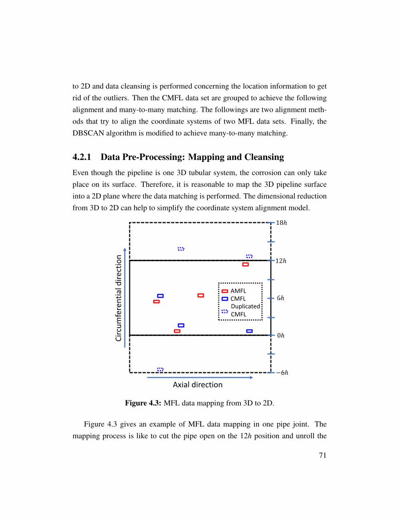
to 2D and data cleansing is performed concerning the location information to getrid of the outliers. Then the CMFL data set are grouped to achieve the followingalignment and many-to-many matching. The followings are two alignment meth-ods that try to align the coordinate systems of two MFL data sets. Finally, theDBSCAN algorithm is modified to achieve many-to-many matching.

4.2.1 Data Pre-Processing: Mapping and CleansingEven though the pipeline is one 3D tubular system, the corrosion can only takeplace on its surface. Therefore, it is reasonable to map the 3D pipeline surfaceinto a 2D plane where the data matching is performed. The dimensional reductionfrom 3D to 2D can help to simplify the coordinate system alignment model.

Axial direction

Cir

cum

fere

nti

al

dir

ect

ion

− ℎ

CMFL

AMFL

Duplicated

CMFL

ℎ

12ℎ

18ℎ

0ℎ

Figure 4.3: MFL data mapping from 3D to 2D.

Figure 4.3 gives an example of MFL data mapping in one pipe joint. Themapping process is like to cut the pipe open on the 12h position and unroll the

71

tubular pipe into a planar surface, marked with the solid black line in Fig. 4.3.However, the box data beside the boundary, 12h, could be separated by the cuttingand the unrolling operations. To address this problem, the 2D plane is extendedto −6h∼ 18h, represented with the dash black line in Fig. 4.3. Besides, one MFLdata set, CMFL in this work, is also duplicated and extended to the whole plane.The duplication can keep all the potentially matched data, while the ones withoutthe corresponding will be filtered out in the following data cleansing operation.

The data cleansing is performed to remove the outliers in both MFL data sets.The outliers denote the box data which have no correspondences in the other dataset. They are resulted from the difference between the detection capabilities oftwo MFL tools and the duplication operation in the previous data mapping. Theexistence of outliers increases the difficulty of data matching and compromisesits accuracy. Herein, the outliers are temporally removed in the matching processto achieve high matching accuracy. However, it doesn’t mean that these data areremoved from the pipeline condition assessment. It will still be analyzed to assessthe integrity of the pipeline in the conventional way where only data from singleMFL is required.

In this research, data cleansing is performed concerning the location infor-mation, namely relative distance and clock position. The study shows that theaccuracy of the location information of MFL tool is ±100mm [214]. Since loca-tion error could exist in both MFL data sets, the maximum distance between thecorresponding box data is 200mm. Therefore, one box data can be regarded as anoutlier and filtered out only when there is no box data from the other MFL dataset within 200mm. The data cleansing is finished by duplicating this step on everysingle data from two MFL data sets.

4.2.2 Grouping the CMFL Box DataBecause of the characteristics of MFL technique, one complicated corrosion areacan be detected and represented with several boxes in the pipe tally file, for ex-ample two box in AMFL while six in CMFL. In this case, the correspondence

72

between two box data sets becomes many-to-many instead of one-to-one. Todeal with the many-to-many matching, the CMFL box data could be grouped asa whole to do the matching with the box data from AMFL. Here, the CMFL dataset is chosen to be grouped because it’s sparse and easy to perform grouping op-eration.

Since the box data should be grouped based on its spatial density, the DB-SCAN algorithm is employed in this research. Besides, the DBSCAN algorithmdoes not require the number of groups to be specified in advance [215]. It regardsthe boxes from MFL as points and groups them based on the density informa-tion. However, the size information, i.e., length and width, can not be fed into theDBSCAN model directly. This is because the DBSCAN treats all the variablesequally and the introduction of size information could group two boxes that arefar from each other just because they share the same size information.

Figure 4.4: Illustration of MFL data grouping.

When only location information is considered in the grouping operation, eachbox is represented with one point locating at its center. The box data that areclosely located with each other will be clustered into one group while the oneswithout adjacencies will be classified as isolated. Since the missing of the sizeinformation, the problem shown in Fig. 4.4 could happen. Box data, d2 and d3,are clustered into different groups just because the distance between their centersis beyond the maximum distance. However, corrosion defect is one area instead ofone point. Even though the distance between the center is beyond the threshold,d2 and d3 should be treated as the adjacent considering their size information.

73

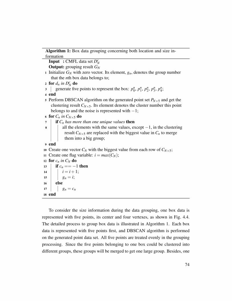
Algorithm 1: Box data grouping concerning both location and size in-formation

Input : CMFL data set DcN

Output: grouping result GN1 Initialize GN with zero vector. Its element, gn, denotes the group number

that the nth box data belongs to;2 for dn in Dc

N do3 generate five points to represent the box: pn

0, pn1, pn

2, pn3, pn

4;4 end5 Perform DBSCAN algorithm on the generated point set PN×5 and get the

clustering result CN×5. Its element denotes the cluster number this pointbelongs to and the noise is represented with −1;

6 for Cn in CN×5 do7 if Cn has more than one unique values then8 all the elements with the same values, except −1, in the clustering

result CN×5 are replaced with the biggest value in Cn to mergethem into a big group;

9 end10 Create one vector CN with the biggest value from each row of CN×5;11 Create one flag variable: i = max(CN);12 for cn in CN do13 if cn ==−1 then14 i = i+1;15 gn = i;16 else17 gn = cn

18 end

To consider the size information during the data grouping, one box data isrepresented with five points, its center and four vertexes, as shown in Fig. 4.4.The detailed process to group box data is illustrated in Algorithm 1. Each boxdata is represented with five points first, and DBSCAN algorithm is performedon the generated point data set. All five points are treated evenly in the groupingprocessing. Since the five points belonging to one box could be clustered intodifferent groups, these groups will be merged to get one large group. Besides, one

74

box will be treated as isolated only when all its five points belong to the noise.The isolated means there is only one box data in this group.

4.2.3 Aligning the Coordinate SystemsDue to the location error associated with individual MFL tool, their coordinatesystems are misaligned. Therefore, direct matching in the misaligned coordinateswould result in inevitable matching error. The coordinate systems of two MFLdata sets must be aligned first before box data matching can be performed. In thischapter, two different alignment methods are proposed and studied; the first oneis based on sliding window search and the other one is based on Gaussian mixturemodel. The transformation function to align two coordinate systems is assumedas affine in this chapter because of the movement coherence in one pipe joint.

Sliding window searching model

For the sliding window searching (SWS) model, the CMFL box data are projectedinto the coordinate system of AMFL data set and slide to maximize the overlaparea between them. Each group of CMFL boxes is treated as one basic alignmentunit. For one CMFL group, one rectangle which can barely cover all the boxes iscreated as the corrosion area and one broader searching area is created surroundingthis corrosion area as shown in Fig. 4.5. The space between two rectangles is200mm which is the maximum distance between the corresponding boxes [214].

The overlapping area sg between two box data sets is recorded as the indicatorof the level of alignment for this basic unit. It is considered as the optimal align-ment location where this overlapping area reaches its maximum during slidinginside the searching area. This operation is duplicated on all CMFL groups. Theoriginal location lg and optimal location l

′g of the corrosion area center of each

group will be recorded and then one global transformation function is derivedfrom them.

The global transformation function aims to minimize the weighted distancesum between the optimal location and the transformed location of each group in

75

CMFL

AMFL

Corrosion area

Searching area

Figure 4.5: Illustration of the sliding window searching model.

the whole pipeline joint. The overlapping area sg is employed as the weight foreach group. The affine transformation matrix B and the translation vector t can bederived with Eq. 4.1:

B, t = argminB,t

G

∑g=1

sg||l′g−Blg− t||2 (4.1)

Gaussian mixture model

Gaussian mixture model (GMM) is one widely used algorithm in point set regis-tration [216, 217]. If each box from two MFL data sets is regarded as one point atits center, ignoring the size information, the alignment of two MFL data sets be-comes the point set registration problem. The box data from AMFL are consideredas the centroids of Gaussian distributions, while the ones from CMFL are treatedas the observations from this Gaussian mixture. The process to align the coordi-nate systems of two point sets is equivalent to maximizing the log-likelihood thatthe observations are sampled from their corresponding Gaussian mixture compo-nents. Following notations are used in this chapter to illustrated the alignmentmethod based on Gaussian mixture model:

• M,N: number of box data from AMFL and CMFL.

76

• XM = (x1,x2, ...,xM)T : location information of the AMFL box data.

• YN = (y1,y2, ...,yN)T : location information of the CMFL box data.

• σ : standard deviation of Gaussian distribution.

Then the log-likelihood function can be illustrated with Eq. 4.2:

Q =M

∑m=1

N

∑n=1

pmnlog(p(yn|m)) (4.2)

where, p(yn|m) means the likelihood that yn is sampled from the mth Gaussianmixture component and it can be calculated with Eq. 4.3:

p(yn|m) =1

2πσ2 exp−||yn−Bxm− t||2

2σ2 (4.3)

Besides, pmn denotes the correspondence probability between mth AMFL boxand nth CMFL box. It is defined as the posterior probability of the mth Gaussianmixture component given the box yn and can be obtained with Eq. 4.4:

pmn =p(yn|m)

∑Mm=1 p(yn|m)

(4.4)

Because of the high computational complexity of log-likelihood function Q,the expectation maximization algorithm is employed to optimize it. First, theaffine transformation matrix B and translation vector t are initialized as identifymatrix and zero vector, respectively. In the expectation step, the correspondenceprobability pmn is updated with Eq. 4.4. In the following maximization step, thecorrespondence probability is assumed to be fixed, then transformation matrix B

and translation vector t can be derived by Newton method with Eq. 4.2. Furtherdetails on this process can be found in [218]. The expectation step and maximiza-tion step will be repeated alternately until the log-likelihood function Q convergesto get the optimal transformation parameters B and t.

77

4.2.4 Matching Box Data in the Aligned Coordinate SystemAfter the alignment of two coordinate systems, data from two MFL tools are pro-jected into the same coordinate space where the box data matching can be per-formed. Box data matching aims to identify the items referring to the same cor-rosion area from two MFL data sets. In this research, the matching is achievedbased on the modified DBSCAN algorithms.

Similar to the aforementioned grouping operation, each box data from MFLis represented with five points, the center and four vertexes, to take both the lo-cation and size information into account. The difference is that instead of onlyone MFL data set, AMFL and CMFL data sets are mixed together to achievebox data matching. Besides, the group information obtained from the aforemen-tioned grouping operation is also applied to achieve many-to-many matching. Thematching process is performed based on the following steps:

• Algorithm 1 is performed on the mixed data set to get the preliminarymatching result.

• If all the members of one group come from only one MFL data set, then thisgroup is treated as outlier.

• All the AMFL box data corresponding to one group of CMFL boxes aremerged into one group to match with the CMFL group.

In the matching operation, the radius of matching has one critical influence onthe matching result. Here, the matching radius is the maximum distance betweentwo samples for one to be considered as in the neighborhood of the other. Theinfluence of matching radius on the result is studied in the experiment 1.

78

4.3 Experimental Results and Discussions

4.3.1 Experimental SetupThe performance of the proposed matching framework was investigated with twofield measured MFL inspection data sets which are provided by our industrialpartner. One in-service pipeline was inspected with their MFL tools and the boxdata were obtained from the acquired MFL signal with their proprietary software.Six pipe joints were selected from the whole pipeline as the test data to evaluatethe performance of the proposed matching framework. For these six pipe joints,box data from two MFL tools were manually matched by human inspectors. Themanually matched results were employed as the reference to evaluate the proposedmatching solution. The details of the six pipe joints are given in Table 4.1:

Table 4.1: Details on the selected six pipe joints.

Joint ID 1560 1570 1780 3160 4750 4760

No. of AMFL boxes 69 44 155 256 657 129No. of CMFL boxes 17 23 17 69 125 37

In our study, the matching also aims to group the data satisfying certain con-ditions together, which is similar to data clustering. Therefore, three objectivemetrics, commonly used to evaluate the performance of clustering algorithms,homogeneity h, completeness c, and V-measure v, are borrowed to conduct objec-tive performance evaluation. These three metrics are proposed by Rosenberg andHirschberg in [219] and their formulations are given in Eq. 4.5:

h = 1− H(C|K)

H(C)(4.5a)

c = 1− H(K|C)

H(K)(4.5b)

79

v = 2 · h · ch+ c

(4.5c)

where, C is the class information of the data set, while K denotes the clusteringresult from the algorithm; H(C|K) denotes the conditional entropy of the classesgiven the cluster assignments; H(K|C) is the conditional entropy of clusters givenclass; H(C) represents the entropy of the classes; and H(K) means the entropy ofclusters .

Homogeneity means that all clusters contain only members of a single class,while completeness suggests that all members of a given class are assigned to thesame cluster. The distance between one matching result and the ideal can be mea-sured as the weighted combination of two metrics, V-measure. For these threemetrics, they all vary from 0 to 1, and the higher value suggests better perfor-mance.

The experiments were conducted on one workstation with the following specs:one Intel Core i9-9820X CPU, two GeForce RTX 2080 Ti GPUs, and 64 GBmemory.

4.3.2 Matching Results with Different RadiiIn this experiment, the performance of the matching framework with differentmatching radii is studied to find out the best matching radii for each alignmentmethod. The matching radius changes from 5mm to 120mm with step 1mm, andwith each step the performance of the matching framework is evaluated in termsof three metrics.

Because of the similarity of their trends, the performance of the Gaussian mix-ture model is illustrated in Fig. 4.6 as one example. With one small matching ra-dius, metric completeness is extremely high while metric homogeneity locates at alow level. The reason behind this phenomenon is that most data are considered asoutliers with a small matching radius. This is because no corresponding data canbe found within the small matching radius. Therefore, the metric completenessis close to 1 since most members of all classes are assigned to the special group

80

20 40 60 80 100 120

Matching radius (mm).

0.4

0.5

0.6

0.7

0.8

0.9

1.0

Score

value.

Completeness

Homogeneity

V-measure

Figure 4.6: Matching performance changes with different matching radii.

‘outlier’. Besides, since the group ‘outlier’ contains members from all differentclasses, the metric homogeneity is relatively low.

With the increase of matching radius, metric completeness drops quickly andthen gradually rises up to 1. However, the other metric homogeneity goes theother way, increasing sharply then gradually dropping. This is because more andmore boxes form their own groups and leave the group ‘outlier’. In the beginning,these newly formed groups are still small and only include parts of their members.This results in the sudden changes of both completeness and homogeneity. Met-ric completeness starts increasing when some groups include all their memberswhile metric homogeneity begins dropping when groups include more than theirmembers.

Because both completeness and homogeneity are important in practical appli-cation, the matching radius maximizing the metric V-measure is regarded as theoptimal radius in this experiment. The optimal matching radii of two alignmentmethods, sliding window searching and Gaussian mixture model, are 48mm and44mm respectively.

81

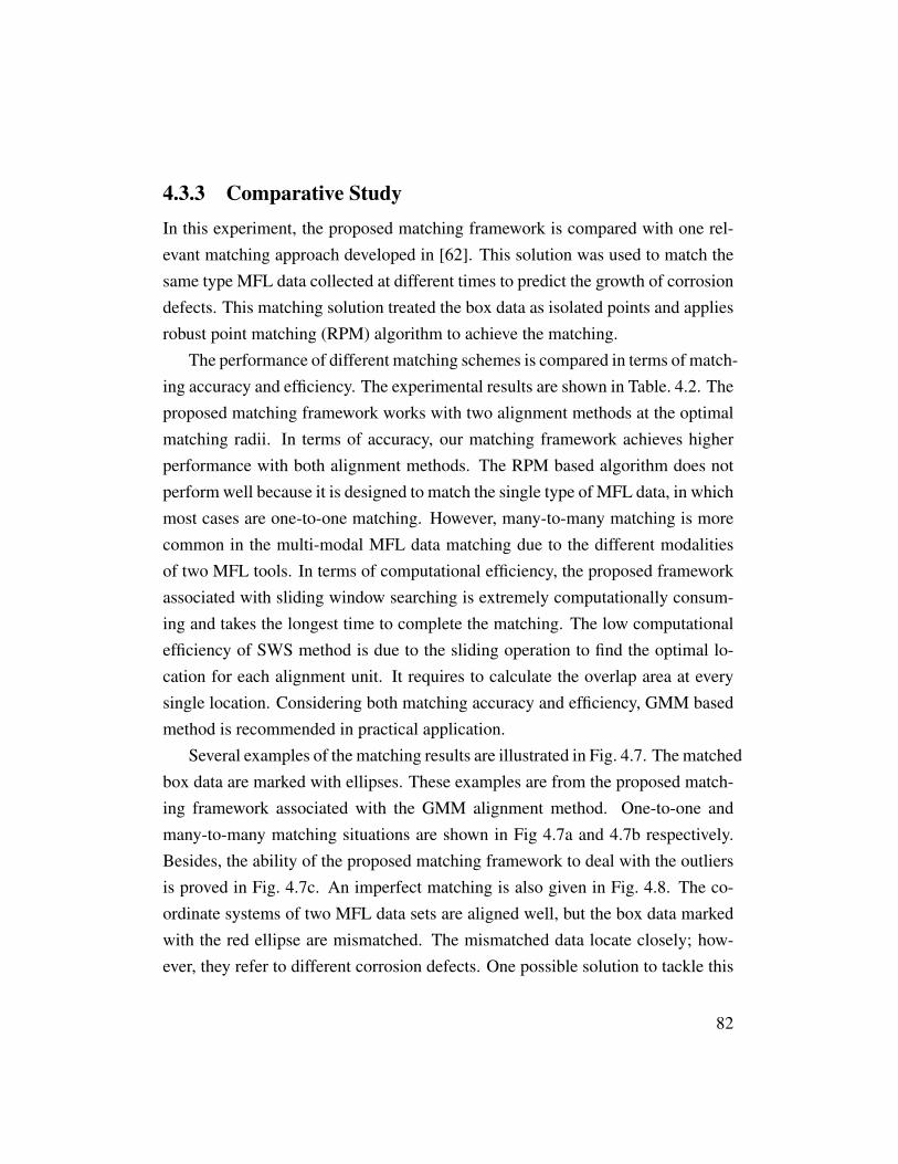
4.3.3 Comparative StudyIn this experiment, the proposed matching framework is compared with one rel-evant matching approach developed in [62]. This solution was used to match thesame type MFL data collected at different times to predict the growth of corrosiondefects. This matching solution treated the box data as isolated points and appliesrobust point matching (RPM) algorithm to achieve the matching.

The performance of different matching schemes is compared in terms of match-ing accuracy and efficiency. The experimental results are shown in Table. 4.2. Theproposed matching framework works with two alignment methods at the optimalmatching radii. In terms of accuracy, our matching framework achieves higherperformance with both alignment methods. The RPM based algorithm does notperform well because it is designed to match the single type of MFL data, in whichmost cases are one-to-one matching. However, many-to-many matching is morecommon in the multi-modal MFL data matching due to the different modalitiesof two MFL tools. In terms of computational efficiency, the proposed frameworkassociated with sliding window searching is extremely computationally consum-ing and takes the longest time to complete the matching. The low computationalefficiency of SWS method is due to the sliding operation to find the optimal lo-cation for each alignment unit. It requires to calculate the overlap area at everysingle location. Considering both matching accuracy and efficiency, GMM basedmethod is recommended in practical application.

Several examples of the matching results are illustrated in Fig. 4.7. The matchedbox data are marked with ellipses. These examples are from the proposed match-ing framework associated with the GMM alignment method. One-to-one andmany-to-many matching situations are shown in Fig 4.7a and 4.7b respectively.Besides, the ability of the proposed matching framework to deal with the outliersis proved in Fig. 4.7c. An imperfect matching is also given in Fig. 4.8. The co-ordinate systems of two MFL data sets are aligned well, but the box data markedwith the red ellipse are mismatched. The mismatched data locate closely; how-ever, they refer to different corrosion defects. One possible solution to tackle this

82

Table 4.2: Comparison between different matching schemes.

Matching schemes Completeness (%) Homogeneity (%) V-measure (%) Time (s)

Robust point matching [62] 86.6 87.8 87.2 2.3Proposed framework (with SWS) 98.8 92.2 95.4 28.4Proposed framework (with GMM) 98.3 92.4 95.2 1.4

83

CMFL

AMFL

(a) One-to-one matching.

CMFL

AMFL

(b) Many-to-many matching.

CMFL

AMFL

(c) Matching with outliers.

Figure 4.7: Examples of successful box data matching results.

84

CMFL

AMFL

Figure 4.8: Example of imperfect box data matching result.

problem is to make use of the signal data for a refined matching when they areavailable.

4.4 SummaryThis chapter proposes a framework to automatically match the multi-modal MFLdata, which is the first-of-its-kind solution. In the experiments, MFL data col-lected from in-service pipeline are used to validate the proposed box data match-ing framework. In terms of the evaluation metrics, the proposed framework canachieve above 95% V-measure value which is much higher than 87.2% achievedby the existing method. Besides, the proposed matching framework with Gaussianmixture model can achieve the best computational efficiency. With the proposedmatching framework, the pipeline inspector can now easily analyze the inspectionresults from two MFL tools, and obtain more comprehensive assessment on thecorrosion defect.

85

Chapter 5

Performance Assessment ofMulti-Modal MFL Inspections usingFeature-based POD

This chapter applies probability of detection (POD) to quantitatively assess thedetection performance of two types of magnetic flux leakage (MFL) inspectionsand their combination. Due to the characteristics of MFL inspection, this chap-ter proposes the construction of the POD model as a function of two geometricvariable, i.e, the volume and the orientation, which have significant influences onthe MFL signal response. Besides, detection results from two MFL tools are in-tegrated using logical OR operation to study the POD of their combination. Withthe proposed POD model, the minimum criteria that ensure a corrosion defect willbe reliably detected by MFL tools are studied. The validity of the proposed PODmodel is justified on the data collected from an in-service pipeline.

5.1 OverviewThe detection performance of non-destructive testing (NDT) techniques can beassessed using POD. It is a probabilistic function which gives the probability

86

that a defect with a size of a can be detected by a certain NDT technique. ThePOD models of ultrasound testing (UT) and eddy current (EC) have been widelystudied [72, 75]. The POD model was first built as a function of the defectsize [73, 74]. They assumed the acquired NDT signals are mostly effected byone defect variable and characterized the defect with this variable. However, usu-ally more than one variable has significant influence on the signal response andcharacterizing the defect with single variable makes it difficult to accurately eval-uate the POD. This problem is addressed in [68, 70, 77], where the POD wasmodelled as the function of the depth and the length of a defect.

Aforementioned studies are on UT and EC. In contrast to that the POD studyfor MFL is quite limited. One research in [79] studied the POD of MFL withrespect to the setups of MFL tools, e.g., liftoff, magnetization level, and sensorspacing. However, the POD in regard to the defect variables is not studied yet.Different from the UT and EC, the signal response of MFL inspection is highlyrelated to the defect volume and orientation. It is only sensitive to the defectcomponent which is perpendicular to its magnetic field. The axial magnetic fluxleakage (AMFL), with circumferential magnetic field, is sensitive to the circum-ferential component of the defect, while the circumferential magnetic flux leakage(CMFL), with axial magnetic field performs well in the axial component detec-tion. Thus, the POD of MFL cannot be evaluated by directly adopting the PODmodels of UT or EC.

In this chapter, the POD models of two different MFL tools are constructedas functions of two geometric variables, i.e., the volume and the orientation ofthe defect, considering the characteristics of MFL inspection. Data analysis sug-gests that higher linearity is achieved with these two variables, which results innarrow confidence bound. Besides, the POD of their combination is also studiedby integrating their inspection results with logical OR operation. The integrationcan address the detection limitation of individual MFL tool on certain defect ori-entations and ensures the corrosion defect with a smaller volume can be reliablydetected.

87

5.2 Probability of Detection ModelIn a non-destructive testing (NDT) system, the signal response, a, is associatedwith the defect variables, a. Their relation can be written as Eq. 5.1:

a = β0 +β1 f (a)+ ε (5.1)

where, f is a function to transform the defect variables, a, to a scalar which islinear to the signal response, a. The coefficients of linear regression, β0 and β1,can be determined by the maximum likelihood method. The variable, ε , denotesthe random variance of measurement which is introduced by the uncontrolled fac-tors in NDT system. In practice, it is assumed to be normally distributed withzero mean and a constant standard deviation, σ , which can be calculated with theresiduals of the experimental data.

A flaw can only be detected when the signal response it causes exceeds thedetection threshold of the NDT system. Therefore, the POD can be calculatedwith Eq. 5.2:

POD = P(a > ath) (5.2)

where, ath is the detection threshold.

5.2.1 Selection of Defect VariablesA critical step in POD evaluation is the determination of the variables to charac-terize the defect. The appropriate defect variables should be able to effectivelyrepresent the corrosion defect. At the same time, it should have a high influenceon the signal response. The depth, area, and volume are three variables that arecommonly used to describe the severity of a corrosion defect. Since the signalresponse of MFL tool is highly related to the defect orientation, the angle betweenthe defect and the pipe axis, θ , is also included in the analysis.

The correlations between the signal response and the defect variables can beevaluated with the Pearson correlation coefficient (PCC), ρ . Its value range is

88

1 2 3 4depth / mm

0

2500

5000

7500

10000 ρ = 0.40

0 1000 2000area / mm2

ρ = 0.59

0 500 1000 1500 2000volume / mm3

ρ = 0.63

0 1 2depth*sin(θ) / mm

0

2500

5000

7500

10000

AMFL_r

espo

nse / nWb

ρ = 0.65

0 500 1000area*sin(θ) / mm2

ρ = 0.71

0 250 500 750 1000volume*sin(θ) / mm3

ρ = 0.90

0 1 2 3 4depth*cos(θ) / mm

0

2500

5000

7500

10000 ρ = 0.10

0 1000 2000area*cos(θ) / mm2

ρ = 0.30

0 1000 2000volume*cos(θ) / mm3

ρ = 0.40

(a) AMFL

1 2 3 4depth / mm

0

5000

10000

15000 ρ = 0.67

0 1000 2000area / mm2

ρ = 0.67

0 500 1000 1500 2000v lume / mm3

ρ = 0.89

0 1 2depth*sin(θ) / mm

0

5000

10000

15000

CMFL_resp

nse / nWb

ρ = -0.02

0 500 1000area*sin(θ) / mm2

ρ = 0.02

0 250 500 750 1000v lume*sin(θ) / mm3

( = 0.31

0 1 2 3 4depth*c s(θ) / mm

0

5000

10000

15000 ( = 0.69

0 1000 2000area*cos(θ) / mm2

ρ = 0.77

0 1000 2000v lume*c s(θ) / mm3

( = 0.93

(b) CMFL

Figure 5.1: Correlation between the signal response and defect variables.

89

between −1 and 1, and higher absolute value denotes better linear correlation.Figure 5.1 illustrates their correlations with the corresponding PCC value shownin the upper left corner of each subplot. The first row is three severity variables,and the following two rows are their circumferential and axial components respec-tively. Take the AMFL as an example, Fig. 5.1a clearly shows that the circumfer-ential components share higher correlations with the signal response, in which thecomponent of volume, vol∗sin(θ), gets the highest PCC value. On the other hand,CMFL is more sensitive to the axial components and the component of volume,vol ∗ cos(θ), achieves the highest PCC value. Therefore, the corrosion defect isrepresented with vol ∗ sin(θ) and vol ∗ cos(θ) in the AMFL and the CMFL PODmodels respectively.

With the determination of the defect variables, the signal response of AMFLand CMFL tools can be calculated with Eq. 5.3 and Eq. 5.4 respectively:

aa = βa0 +βa1 ∗ vol ∗ sin(θ)+ εa (5.3)

ac = βc0 +βc1 ∗ vol ∗ cos(θ)+ εc (5.4)

5.2.2 POD Combination of Multiple MFL InspectionsIn pipeline industry, two types of MFL tools are employed in the in-line inspec-tion. The detection results from two MFL tools can be integrated for improveddetection capability due to their complementary measurement properties. In thisstudy, logical OR operation is introduced to conduct the integration. A corrosiondefect is believed to be detectable when it is detected by either MFL tool. Thus,the POD of the combination can be expressed with Eq. 5.5:

PODcombi = P(aa > aath || ac > acth) (5.5)

The calculation can be simplified by introducing the complementary event,which is the corrosion defect is missed by two MFL tools at the same time. Since

90

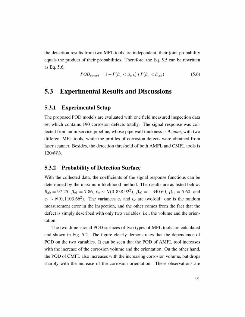
the detection results from two MFL tools are independent, their joint probabilityequals the product of their probabilities. Therefore, the Eq. 5.5 can be rewrittenas Eq. 5.6:

PODcombi = 1−P(aa < aath)∗P(ac < acth) (5.6)

5.3 Experimental Results and Discussions

5.3.1 Experimental SetupThe proposed POD models are evaluated with one field measured inspection dataset which contains 190 corrosion defects totally. The signal response was col-lected from an in-service pipeline, whose pipe wall thickness is 9.5mm, with twodifferent MFL tools, while the profiles of corrosion defects were obtained fromlaser scanner. Besides, the detection threshold of both AMFL and CMFL tools is120nWb.

5.3.2 Probability of Detection SurfaceWith the collected data, the coefficients of the signal response functions can bedetermined by the maximum likelihood method. The results are as listed below:βa0 = 97.25, βa1 = 7.86, εa ∼ N(0,838.922), βc0 = −340.60, βc1 = 5.60, andεc ∼ N(0,1103.662). The variances εa and εc are twofold: one is the randommeasurement error in the inspection, and the other comes from the fact that thedefect is simply described with only two variables, i.e., the volume and the orien-tation.

The two dimensional POD surfaces of two types of MFL tools are calculatedand shown in Fig. 5.2. The figure clearly demonstrates that the dependence ofPOD on the two variables. It can be seen that the POD of AMFL tool increaseswith the increase of the corrosion volume and the orientation. On the other hand,the POD of CMFL also increases with the increasing corrosion volume, but dropssharply with the increase of the corrosion orientation. These observations are

91

orientation / °

6080 Def

e

m3

0250

0000

Pro

bability o

f dete

ction / %

50

60

70

80

90

100

(a) AMFL

orientation / °

6080 Def

e

m3

0250

0000

Pro

bability o

f dete

ction / %

40

50

60

70

80

90

100

(b) CMFL

Figure 5.2: POD surface of individual MFL tool.

92

consistent with the detection characteristics of MFL tools as they are good atdetecting corrosion defects which are perpendicular to their magnetic field.

0 500 1000 1500 2000Defect volume / mm3

0

20

40

60

80De

fect

orie

ntat

ion

/ °POD = 90%Lower 95% confidence bound

(a) AMFL

0 500 1000 1500 2000Defect volume / mm3

0

20

40

60

80

Defe

ct o

rient

atio

n / °

POD = 90%Lower 95% confidence bound

(b) CMFL

Figure 5.3: POD = 90% and its 95% confidence bound.

In POD application, a90/95 is a generally used criterion. It is believed that theflaws satisfying this condition can be reliably detected. The value a90/95 repre-sents the condition that a 90% POD can be reached with a 95% confidence level.

93

In this research, the POD is a function of two defect variables. Therefore, thea90/95 is a curve and can be illustrated with Fig. 5.3. The solid line representsthe condition where POD can reach 90%, and the dashed line denotes its lower95% confidence bound. The defects locating on its right side are believed to bereliably detected. The narrow confidence bound is because of the high linearity ofthe proposed POD model.

0 100 200 300 400 500Defect volume / mm3

0

10

20

30

40

50

60

70

80

90

Defect orie

ntat

ion / °

AMFLCMFLCombination

Figure 5.4: POD = 90% curve of multi-modal MFL combination.

The POD of individual MFL tool shows their limitation on detecting the cor-rosion defects with certain orientations. This limitation can be overcome by thecombination of AMFL and CMFL, and the result is shown in Fig. 5.4. It showsthat the combination have a high POD for corrosion defects with all orientations.Inspection with two MFL tools can reliably detect any corrosion defect with vol-ume greater than 47mm3.

94

5.4 SummaryIn this chapter, the POD model of MFL inspection for pipeline is constructed withtwo geometric variables of a corrosion defect, i.e., the volume and the orienta-tion, as they both have significant influences on the MFL signal response and thepipeline structural integrity. In comparison with the individual variable, the factorconsisting of two variables achieves a higher correlation with the signal response.With the proposed POD model, the minimum criteria for a corrosion defect to bereliably detected are quantitatively identified. Besides, the inspection results frommultiple MFL tools are combined in this study to address the detection limitationof individual MFL tool on certain defect orientations. The integration results showthat any corrosion defect whose volume is greater than 47mm3 will be reliably de-tected.

95

Chapter 6

Conclusions

In this thesis, the magnetic flux leakage (MFL) data collected from in-line inspec-tion are analyzed to facilitate the decision-making process in the pipeline integritymanagement program.

To obtain a contextual representation of the corrosion defect, the concept ofparameterization is put forward in Chapter 3. Three parameterization models, i.e.,principal component analysis, convolutional auto-encoder, and shape context, aredeveloped. The extracted contextual representation enables similar defect retrievaland defect population analysis. Similar defect retrieval can help to identify thesimilar defects which pose a serious threat to the pipeline integrity, and defectpopulation analysis gives an overall assessment of all the corrosion defects in apipeline.

To automatically match the inspection data from different tools, i.e., axialMFL and circumferential MFL, a computational framework is proposed in Chap-ter 4. The proposed framework consists of four major steps: pre-processing,grouping, alignment, and matching. It can identify the inspection data referring tothe same corrosion defects. Because of the complementary detection capabilitiesof two MFL tools, the structural engineers can analyze matched data and have acomprehensive understanding of the corrosion defect.

The detection performance of MFL inspection is quantitatively assessed using

96

a probability of detection (POD) model in Chapter 5. With the proposed PODmodel, the possibility of a defect being detected and/or missed can be calculated.It helps the structural engineers obtain an assessment on the undetected defects inthe inspection.

To sum up, the research outcomes presented in this thesis can help structuralengineers quickly identify the pipeline threat, easily access all the inspection re-sults of a certain defect, and even obtain an assessment on the undetected defectsin the inspection. Based on the outcomes, the structural engineers can make theappropriate decision to maintain the pipeline integrity effectively and economi-cally.

6.1 ContributionsThe main contributions of this thesis research are summarized as follows.

• The concept of parameterization is put forward to obtain a contextual rep-resentation of corrosion defects. In parameterization, the adjacent defectsare considered as the additional information of the central one. The pro-posed shape context based model is proved to outperform other two mod-els, i.e., principal component analysis based and convolutional auto-encoderbased models. Besides, a two-dimensional Gaussian function is introducedto model the interaction strength between adjacent defects, and it furtherimproves the model accuracy.

• The proposed multi-modal MFL data matching framework incorporates asliding window searching approach and a Gaussian mixture model to alignthe coordinate systems of two data sets for improved accuracy and effi-ciency, respectively. The density-based spatial clustering of applicationswith noise algorithm is modified to take both the location and the size infor-mation into account. Higher matching accuracy is achieved due to the intro-duction of the size information. Besides, the proposed matching framework

97

works on the box data derived from MFL inspection, and can be potentiallyapplied to any other non-destructive testing data.

• The proposed POD model is constructed with two geometric variables of acorrosion defect, i.e., the volume and the orientation. In comparison withthe individual variable, the factor consisting of the two variables achieves ahigher correlation with the signal response. Besides, the inspection resultsfrom multiple MFL tools are integrated to take advantage of their comple-mentary detection capabilities, and eventually address the detection limita-tions on certain defect orientations.

6.2 Limitations and Future WorkThe proposed models in this study have proved their effectiveness in the pipelineintegrity management program. The limitations and the potential future work ofthis research are discussed and listed as below.

• In corrosion defect parameterization, the interaction strength between ad-jacent defects is modeled with a two-dimensional Gaussian function. Theparameters of this function are set empirically while they could be effectedby the settings and operation conditions of the MFL tools. Following re-search could conduct simulation or experiment to further study the interac-tion strength. Besides, the contextual information contained in the extractedparameterization vector makes it a perfect input to estimate the pipe failurepressure. Therefore, pipe failure pressure estimation could be another ap-plication of corrosion defect parameterization.

• The proposed MFL data matching framework works on the box data whilehow to achieve signal matching is still an open research topic. When thesignal data are available, signal matching can achieve higher accuracy dueto the detailed information contained in the signal data. However, signalmatching remains a challenge because the signals from two types of MFL

98

tools look differently. One potential solution is to translate the MFL signalsto the same domain where they share more similarities. This translationoperation can be achieved using image translation technique which requiresthe matched signal data for training. After the translation is done, templatematching technique could be employed to match the signals in the samedomain.

• The proposed POD model quantitatively assesses the detection performanceof MFL inspection concerning the volume and the orientation of a defect.Other defect variables, e.g., the depth and the area, are ignored due to thelimited size of the data set. With more data become available, these vari-ables could be considered to describe the corrosion defect more precisely.The relationship between the MFL signal response and the corrosion de-fect can be modelled with higher accuracy. Eventually, the detection per-formance of MFL inspection on more specific corrosion variables can beassessed.

Besides the topics covered in this thesis, the 3D profile reconstruction of corro-sion defect is another interesting direction for the future research. The 3D profileof a corrosion defect can benefit an accurate pipeline structure safety analysis andan effective maintenance prioritization. However, current inspect results are pre-sented to the structural engineers in the form of box data while the true shape ofthe corrosion defect is unknown. Future research could fuse the signal data fromtwo types of MFL tools, and employ fully convolutional encoder-decoder networkto achieve the 3D profile reconstruction of corrosion defects.

99

Bibliography

[1] “Oil pipelines,”https://www.oilsandsmagazine.com/projects/crude-oil-liquids-pipelines,accessed Mar. 05, 2021. → pages xiii, 2

[2] “Intelligent pigging pipeline inspection services oil & gas industry,”www.https://www.youtube.com/watch?v=rmJ083afaYY, accessed Mar.028, 2021. → pages xiii, 6

[3] K. Siggers, “In-line inspection - guest lecture,” University Lecture, 2017.→ pages xiii, 7, 8

[4] Q. Zhou, W. Wu, D. Liu, K. Li, and Q. Qiao, “Estimation of corrosionfailure likelihood of oil and gas pipeline based on fuzzy logic approach,”Engineering Failure Analysis, vol. 70, pp. 48–55, Dec. 2016. [Online].Available: https://doi.org/10.1016/j.engfailanal.2016.07.014 → page 1

[5] X. Peng, U. Anyaoha, Z. Liu, and K. Tsukada, “Analysis of magnetic-fluxleakage (MFL) data for pipeline corrosion assessment,” IEEETransactions on Magnetics, vol. 56, no. 6, pp. 1–15, Jun. 2020. [Online].Available: https://doi.org/10.1109/tmag.2020.2981450 → pages 1, 67

[6] “Pipelines across canada,” https://www.nrcan.gc.ca/our-natural-resources/energy-sources-distribution/clean-fossil-fuels/pipelines/pipelines-across-canada/18856, accessed Mar.05, 2021. → page 1

[7] J. F. Murphy, “Nightmare pipeline failures, fantasy planning, black swans,and integrity management - a review,” Process Safety Progress, vol. 34,no. 2, pp. 207–207, May 2015. [Online]. Available:https://doi.org/10.1002/prs.11744 → page 1

100

[8] “Pipeline incident 20 year trends,” https://www.phmsa.dot.gov/, accessedon Dec. 19, 2018. → page 1

[9] Z. Usarek and K. Warnke, “Inspection of gas pipelines using magnetic fluxleakage technology,” Advances in Materials Science, vol. 17, no. 3, pp.37–45, Sep. 2017. [Online]. Available:https://doi.org/10.1515/adms-2017-0014 → page 1

[10] C. I. Ossai, B. Boswell, and I. J. Davies, “Pipeline failures in corrosiveenvironments – a conceptual analysis of trends and effects,” EngineeringFailure Analysis, vol. 53, pp. 36–58, Jul. 2015. [Online]. Available:https://doi.org/10.1016/j.engfailanal.2015.03.004 → page 1

[11] “Natural gas pipelines challenges,”https://www.npc.org/Prudent Development-Topic Papers/2-19 Gas Pipeline Challenges Paper.pdf, accessed Mar. 05, 2021. →page 1

[12] S. Shin, G. Lee, U. Ahmed, Y. Lee, J. Na, and C. Han, “Risk-basedunderground pipeline safety management considering corrosion effect,”Journal of Hazardous Materials, vol. 342, pp. 279–289, Jan. 2018.[Online]. Available: https://doi.org/10.1016/j.jhazmat.2017.08.029 →page 1

[13] A. A. Olajire, “Corrosion inhibition of offshore oil and gas productionfacilities using organic compound inhibitors - a review,” Journal ofMolecular Liquids, vol. 248, pp. 775–808, Dec. 2017. [Online]. Available:https://doi.org/10.1016/j.molliq.2017.10.097 → page 1

[14] F. Shi, X. Peng, Z. Liu, E. Li, and Y. Hu, “A data-driven approach for pipedeformation prediction based on soil properties and weather conditions,”Sustainable Cities and Society, vol. 55, p. 102012, Apr. 2020. [Online].Available: https://doi.org/10.1016/j.scs.2019.102012 → page 1

[15] H. Wang, “Modelling of external corrosion propagation for buriedpipelines based on stochastic processes,” Ph.D. dissertation, University ofAkron, 2015. → page 2

[16] T. Wenman and J. Dim, “Pipeline integrity management,” in All Days.SPE, Nov. 2012. [Online]. Available: https://doi.org/10.2118/161948-ms→ page 2

101

[17] R. Goodfellow and K. Jonsson, “Pipeline integrity management systems(PIMS),” in Oil and Gas Pipelines. John Wiley & Sons, Inc., Apr. 2015,pp. 1–12. [Online]. Available:https://doi.org/10.1002/9781119019213.ch01

[18] H. Iqbal, B. Waheed, S. Tesfamariam, and R. Sadiq, “IMPAKT: Oil andgas pipeline integrity management program assessment,” Journal ofPipeline Systems Engineering and Practice, vol. 9, no. 3, p. 06018003,Aug. 2018. [Online]. Available:https://doi.org/10.1061/(asce)ps.1949-1204.0000326 → page 2

[19] “The pipeline integrity management program (imp) compliance assurancesummary,” https://www.bcogc.ca/files/reports/Annual-Reports/2017-pipeline-imp-report.pdf, accessed Feb. 22, 2021. → page 2

[20] S. Hassanien, L. Leblanc, and A. Nemeth, “Towards an acceptablepipeline integrity target reliability,” in Volume 2: Pipeline SafetyManagement Systems; Project Management, Design, Construction andEnvironmental Issues; Strain Based Design; Risk and Reliability;Northern Offshore and Production Pipelines. American Society ofMechanical Engineers, Sep. 2016. [Online]. Available:https://doi.org/10.1115/ipc2016-64425 → page 2

[21] L. LeBlanc, W. Kresic, S. Keane, and J. Munro, “Advanced integritymanagement framework for pipelines,” in Volume 1: Pipelines andFacilities Integrity. American Society of Mechanical Engineers, Sep.2016. [Online]. Available: https://doi.org/10.1115/ipc2016-64609 →pages 2, 5

[22] H. A. Gabbar and H. A. Kishawy, “Framework of pipeline integritymanagement,” International Journal of Process Systems Engineering,vol. 1, no. 3/4, p. 215, 2011. [Online]. Available:https://doi.org/10.1504/ijpse.2011.041560 → page 3

[23] M. Xie and Z. Tian, “A review on pipeline integrity management utilizingin-line inspection data,” Engineering Failure Analysis, vol. 92, pp.222–239, Oct. 2018. [Online]. Available:https://doi.org/10.1016/j.engfailanal.2018.05.010 → page 3

102

[24] F. Brichau and J. Deconinck, “A numerical model for cathodic protectionof buried pipes,” CORROSION, vol. 50, no. 1, pp. 39–49, Jan. 1994.[Online]. Available: https://doi.org/10.5006/1.3293492 → page 5

[25] X. Chen, X. Li, C. Du, and Y. Cheng, “Effect of cathodic protection oncorrosion of pipeline steel under disbonded coating,” Corrosion Science,vol. 51, no. 9, pp. 2242–2245, Sep. 2009. [Online]. Available:https://doi.org/10.1016/j.corsci.2009.05.027

[26] S. A. Shipilov and I. L. May, “Structural integrity of aging buriedpipelines having cathodic protection,” Engineering Failure Analysis,vol. 13, no. 7, pp. 1159–1176, Oct. 2006. [Online]. Available:https://doi.org/10.1016/j.engfailanal.2005.07.008 → page 5

[27] H. Vanaei, A. Eslami, and A. Egbewande, “A review on pipelinecorrosion, in-line inspection (ILI), and corrosion growth rate models,”International Journal of Pressure Vessels and Piping, vol. 149, pp. 43–54,Jan. 2017. [Online]. Available: https://doi.org/10.1016/j.ijpvp.2016.11.007→ pages 5, 24

[28] H. A. Kishawy and H. A. Gabbar, “Review of pipeline integritymanagement practices,” International Journal of Pressure Vessels andPiping, vol. 87, no. 7, pp. 373–380, Jul. 2010. [Online]. Available:https://doi.org/10.1016/j.ijpvp.2010.04.003 → pages 5, 24

[29] R. Bickerstaff, M. Vaughn, G. Stoker, M. Hassard, and M. Garrett,“1review of sensor technologies for in-line inspection of natural gaspipelines,” 2002. → page 6

[30] H. Song, L. Yang, G. Liu, G. Tian, D. Ona, Y. Song, and S. Li,“Comparative analysis of in-line inspection equipments and technologies,”IOP Conference Series: Materials Science and Engineering, vol. 382, p.032021, Jul. 2018. [Online]. Available:https://doi.org/10.1088/1757-899x/382/3/032021 → page 6

[31] Z. Wang, Y. Gu, and Y. Wang, “A review of three magnetic NDTtechnologies,” Journal of Magnetism and Magnetic Materials, vol. 324,no. 4, pp. 382–388, Feb. 2012. [Online]. Available:https://doi.org/10.1016/j.jmmm.2011.08.048 → page 7

103

[32] H. M. Kim and G. S. Park, “A study on the estimation of the shapes ofaxially oriented cracks in CMFL type NDT system,” IEEE Transactionson Magnetics, vol. 50, no. 2, pp. 109–112, Feb. 2014. [Online]. Available:https://doi.org/10.1109/tmag.2013.2283343 → pages 7, 67

[33] P. C. Porter, “Use of magnetic flux leakage (MFL) for the inspection ofpipelines and storage tanks,” in Nondestructive Evaluation of AgingUtilities, W. G. Reuter, Ed. SPIE, May 1995. [Online]. Available:https://doi.org/10.1117/12.209361 → page 7

[34] T. Bubenik, “Electromagnetic methods for detecting corrosion inunderground pipelines: magnetic flux leakage (MFL),” in UndergroundPipeline Corrosion. Elsevier, 2014, pp. 215–226. [Online]. Available:https://doi.org/10.1533/9780857099266.2.215 → page 7

[35] Y. Shi, C. Zhang, R. Li, M. Cai, and G. Jia, “Theory and application ofmagnetic flux leakage pipeline detection,” Sensors, vol. 15, no. 12, pp.31 036–31 055, Dec. 2015. [Online]. Available:https://doi.org/10.3390/s151229845 → pages 7, 32

[36] F. Wang, Q. Feng, and L. Zhou, “Application progress of tri-axial MFLsensors technology,” in ICPTT 2011. American Society of CivilEngineers, Oct. 2011. [Online]. Available:https://doi.org/10.1061/41202(423)104 → page 7

[37] J. Walker, In-line inspection of pipelines: advanced technologies foreconomic and safe operation of oil and gas pipelines. Verl. ModerneIndustrie, 2010. → page 7

[38] X. Peng, C. Zhang, U. Anyaoha, K. Siggers, and Z. Liu, “Parameterizingmagnetic flux leakage data for pipeline corrosion defect retrieval,” in 2019IEEE 28th International Symposium on Industrial Electronics (ISIE).IEEE, Jun. 2019. [Online]. Available:https://doi.org/10.1109/isie.2019.8781224 → pages 7, 38

[39] M. Witek, “Validation of in-line inspection data quality and impact onsteel pipeline diagnostic intervals,” Journal of Natural Gas Science andEngineering, vol. 56, pp. 121–133, Aug. 2018. [Online]. Available:https://doi.org/10.1016/j.jngse.2018.05.036 → page 7

104

[40] A. Lopes, “Mechanical damage assessment using multiple data sets ininline inspection,” in 8th Pipeline Technology Conference 2013. EITEPInstitute, 2013. → pages 7, 10

[41] M. Kirkwood, “Overcoming limitations of current in-line inspectiontechnology by applying a new approach using spiral magnetic flux leakage(smfl),” in 6th Pipeline Technology Conference 2011. EITEP Institute,2015. → pages 7, 10

[42] M. Miyahara and Y. Yoshida, “Mathematical transform of (r, g, b) colordata to munsell (h, v, c) color data,” in Visual Communications and ImageProcessing '88: Third in a Series, T. R. Hsing, Ed. SPIE, Oct. 1988.[Online]. Available: https://doi.org/10.1117/12.969009 → page 14

[43] J. S. Weszka, C. R. Dyer, and A. Rosenfeld, “A comparative study oftexture measures for terrain classification,” IEEE Transactions on Systems,Man, and Cybernetics, vol. SMC-6, no. 4, pp. 269–285, 1976. [Online].Available: https://doi.org/10.1109/tsmc.1976.5408777 → page 14

[44] M. A. Stricker and M. Orengo, “Similarity of color images,” in Storageand Retrieval for Image and Video Databases III, W. Niblack and R. C.Jain, Eds. SPIE, Mar. 1995. [Online]. Available:https://doi.org/10.1117/12.205308 → page 14

[45] J. Smith and S.-F. Chang, “Automated binary texture feature sets for imageretrieval,” in 1996 IEEE International Conference on Acoustics, Speech,and Signal Processing Conference Proceedings. IEEE, 1996. [Online].Available: https://doi.org/10.1109/icassp.1996.545867 → page 14

[46] R. M. Haralick, K. Shanmugam, and I. Dinstein, “Textural features forimage classification,” IEEE Transactions on Systems, Man, andCybernetics, vol. SMC-3, no. 6, pp. 610–621, Nov. 1973. [Online].Available: https://doi.org/10.1109/tsmc.1973.4309314 → page 14

[47] Y. Rui, A. C. She, and T. S. Huang, “Modified fourier descriptors forshape representation – a practical approach,” in PROC OF FIRSTINTERNATIONAL WORKSHOP ON IMAGE DATABASES AND MULTIMEDIA SEARCH, 1996. → page 14

[48] C. T. Zahn and R. Z. Roskies, “Fourier descriptors for plane closedcurves,” IEEE Transactions on Computers, vol. C-21, no. 3, pp. 269–281,

105

Mar. 1972. [Online]. Available: https://doi.org/10.1109/tc.1972.5008949→ page 14

[49] E. Persoon and K.-S. Fu, “Shape discrimination using fourier descriptors,”IEEE Transactions on Systems, Man, and Cybernetics, vol. 7, no. 3, pp.170–179, 1977. [Online]. Available:https://doi.org/10.1109/tsmc.1977.4309681 → page 14

[50] M.-K. Hu, “Visual pattern recognition by moment invariants,” IEEETransactions on Information Theory, vol. 8, no. 2, pp. 179–187, Feb. 1962.[Online]. Available: https://doi.org/10.1109/tit.1962.1057692 → page 14

[51] D. Kapur, Y. Lakshman, and T. Saxena, “Computing invariants usingelimination methods,” in Proceedings of International Symposium onComputer Vision - ISCV. IEEE Comput. Soc. Press, 1995. [Online].Available: https://doi.org/10.1109/iscv.1995.476984 → page 14

[52] L. Yang and F. Albregtsen, “Fast computation of invariant geometricmoments: a new method giving correct results,” in Proceedings of 12thInternational Conference on Pattern Recognition. IEEE Comput. Soc.Press, 1994. [Online]. Available: https://doi.org/10.1109/icpr.1994.576257→ page 14

[53] Y. Bengio, “Learning deep architectures for AI,” Foundations andTrends® in Machine Learning, vol. 2, no. 1, pp. 1–127, 2009. [Online].Available: https://doi.org/10.1561/2200000006 → page 15

[54] Y. LeCun, Y. Bengio, and G. Hinton, “Deep learning,” Nature, vol. 521,no. 7553, pp. 436–444, May 2015. [Online]. Available:https://doi.org/10.1038/nature14539 → page 15

[55] A. Krizhevsky, I. Sutskever, and G. E. Hinton, “ImageNet classificationwith deep convolutional neural networks,” Communications of the ACM,vol. 60, no. 6, pp. 84–90, May 2017. [Online]. Available:https://doi.org/10.1145/3065386 → page 15

[56] K. Simonyan and A. Zisserman, “Very deep convolutional networks forlarge-scale image recognition,” in 3rd International Conference onLearning Representations, ICLR 2015, San Diego, CA, USA, May 7-9,2015, Conference Track Proceedings, Y. Bengio and Y. LeCun, Eds.,2015. [Online]. Available: http://arxiv.org/abs/1409.1556 → page 15

106

[57] K. He, X. Zhang, S. Ren, and J. Sun, “Deep residual learning for imagerecognition,” in 2016 IEEE Conference on Computer Vision and PatternRecognition (CVPR). IEEE, Jun. 2016. [Online]. Available:https://doi.org/10.1109/cvpr.2016.90 → page 15

[58] C. Champlin and J. P. Steele, “Robust anomaly matching for icips:Reducing pipeline assessment uncertainty through 4-dimensional anomalydetection and characterization,” Colorado School of Mines, Tech. Rep.,2016. → pages 15, 16

[59] J. Palmer, A. Miller, and J. Knudsen, “Automated signal comparison andnormalization - an advanced method of comparing repeat ili data,” in 29thPipeline Pigging & Integrity Management Conference. ClarionTechnical Conferences, 2017. → pages 15, 68

[60] J. Dawson and L. Ganim, “Predicting the future-applying corrosiongrowth rates derived from repeat ili runs,” in 11th Pipeline TechnologyConference 2016. EITEP Institute, 2016. → page 16

[61] I. Cvitanovic, U. Thuenemann, C. Argent, C. Lyons, and A. Wilde,“Development of integrity management strategies for pipelines,” in 5thPipeline Technology Conference 2010. EITEP Institute, 2011. → page16

[62] M. R. Dann and C. Dann, “Automated matching of pipeline corrosionfeatures from in-line inspection data,” Reliability Engineering & SystemSafety, vol. 162, pp. 40–50, Jun. 2017. [Online]. Available:https://doi.org/10.1016/j.ress.2017.01.008 → pages 16, 68, 82, 83

[63] P. Besl and N. D. McKay, “A method for registration of 3-d shapes,” IEEETransactions on Pattern Analysis and Machine Intelligence, vol. 14, no. 2,pp. 239–256, Feb. 1992. [Online]. Available:https://doi.org/10.1109/34.121791 → page 16

[64] H. Liu, Z. Liu, B. Taylor, and H. Dong, “Matching pipeline in-lineinspection data for corrosion characterization,” NDT & E International,vol. 101, pp. 44–52, Jan. 2019. [Online]. Available:https://doi.org/10.1016/j.ndteint.2018.10.004 → pages 16, 68

[65] G. Desjardins, R. Nickle, D. Skibinsky, and J. Yip, “Comparison of in-lineinspection service provider magnetic flux leakage (MFL) technology and

107

analytical performance based on multiple runs on pipeline segments,” inVolume 2: Pipeline Integrity Management. American Society ofMechanical Engineers, Sep. 2012. [Online]. Available:https://doi.org/10.1115/ipc2012-90251 → page 17

[66] A. Russell, M. Smith, D. Sandana, and J. Knudsen, “Advances in magneticflux leakage signal matching and corrosion growth rate selection,” inPigging Products & Services Association, 2016. → page 17

[67] P. J. Moreno, M. A. Ellinger, and T. A. Bubenik, “ILI to ILI comparisons:Quantifying the impact of multiple inspections,” in Volume 1: Pipelinesand Facilities Integrity. American Society of Mechanical Engineers,Sep. 2016. [Online]. Available: https://doi.org/10.1115/ipc2016-64547 →pages 17, 68

[68] N. Yusa, W. Chen, and H. Hashizume, “Demonstration of probability ofdetection taking consideration of both the length and the depth of a flawexplicitly,” NDT & E International, vol. 81, pp. 1–8, Jul. 2016. [Online].Available: https://doi.org/10.1016/j.ndteint.2016.03.001 → pages 17, 87

[69] E. C. J. R. C. I. for Energy., Probability of detection curves :statistical bestpractices. Publications Office, 2010. [Online]. Available:https://data.europa.eu/doi/10.2790/21826 → page 17

[70] M. Pavlovic, K. Takahashi, and C. Muller, “Probability of detection as afunction of multiple influencing parameters,” Insight - Non-DestructiveTesting and Condition Monitoring, vol. 54, no. 11, pp. 606–611, Nov.2012. [Online]. Available: https://doi.org/10.1784/insi.2012.54.11.606 →pages 17, 87

[71] J. S. Knopp, R. Grandhi, J. C. Aldrin, and I. Park, “Statistical analysis ofeddy current data from fastener site inspections,” Journal ofNondestructive Evaluation, vol. 32, no. 1, pp. 44–50, Oct. 2012. [Online].Available: https://doi.org/10.1007/s10921-012-0157-5 → page 17

[72] J. H. Kurz, A. Jungert, S. Dugan, G. Dobmann, and C. Boller, “Reliabilityconsiderations of NDT by probability of detection (POD) determinationusing ultrasound phased array,” Engineering Failure Analysis, vol. 35, pp.609–617, Dec. 2013. [Online]. Available:https://doi.org/10.1016/j.engfailanal.2013.06.008 → pages 17, 87

108

[73] J. Zhu, Q. Min, J. Wu, and G. Y. Tian, “Probability of detection for eddycurrent pulsed thermography of angular defect quantification,” IEEETransactions on Industrial Informatics, vol. 14, no. 12, pp. 5658–5666,Dec. 2018. [Online]. Available: https://doi.org/10.1109/tii.2018.2866443→ pages 17, 87

[74] Y. Duan, H. Zhang, X. P. Maldague, C. Ibarra-Castanedo, P. Servais,M. Genest, S. Sfarra, and J. Meng, “Reliability assessment of pulsedthermography and ultrasonic testing for impact damage of CFRP panels,”NDT & E International, vol. 102, pp. 77–83, Mar. 2019. [Online].Available: https://doi.org/10.1016/j.ndteint.2018.11.010 → pages 17, 87

[75] L. L. Gratiet, B. Iooss, G. Blatman, T. Browne, S. Cordeiro, andB. Goursaud, “Model assisted probability of detection curves: Newstatistical tools and progressive methodology,” Journal of NondestructiveEvaluation, vol. 36, no. 1, Dec. 2016. [Online]. Available:https://doi.org/10.1007/s10921-016-0387-z → pages 18, 87

[76] L. Gandossi and K. Simola, “Derivation and use of probability of detectioncurves in the nuclear industry,” Insight - Non-Destructive Testing andCondition Monitoring, vol. 52, no. 12, pp. 657–663, Dec. 2010. [Online].Available: https://doi.org/10.1784/insi.2010.52.12.657 → page 18

[77] N. Yusa and J. S. Knopp, “Evaluation of probability of detection (POD)studies with multiple explanatory variables,” Journal of Nuclear Scienceand Technology, vol. 53, no. 4, pp. 574–579, Jul. 2015. [Online].Available: https://doi.org/10.1080/00223131.2015.1064332 → pages18, 87

[78] R. Jarvis, P. Cawley, and P. B. Nagy, “Performance evaluation of amagnetic field measurement NDE technique using a model assistedprobability of detection framework,” NDT & E International, vol. 91, pp.61–70, Oct. 2017. [Online]. Available:https://doi.org/10.1016/j.ndteint.2017.06.006 → page 18

[79] Z. Zeng, L. Xuan, Y. Sun, L. Udpa, and S. Udpa, “PROBABILITY OFDETECTION MODEL FOR GAS TRANSMISSION PIPELINEINSPECTION,” Research in Nondestructive Evaluation, vol. 15, no. 3, pp.99–110, Jul. 2004. [Online]. Available:https://doi.org/10.1080/09349840490480756 → pages 18, 87

109

[80] A. Benmoussa, M. Hadjel, and M. Traisnel, “Corrosion behavior of API 5lx-60 pipeline steel exposed to near-neutral pH soil simulating solution,”Materials and Corrosion, vol. 57, no. 10, pp. 771–777, Oct. 2006.[Online]. Available: https://doi.org/10.1002/maco.200503964 → page 23

[81] S. Nesic, “Key issues related to modelling of internal corrosion of oil andgas pipelines – a review,” Corrosion Science, vol. 49, no. 12, pp.4308–4338, Dec. 2007. [Online]. Available:https://doi.org/10.1016/j.corsci.2007.06.006 → pages 24, 40

[82] H. Wang, A. Yajima, R. Y. Liang, and H. Castaneda, “Bayesian modelingof external corrosion in underground pipelines based on the integration ofmarkov chain monte carlo techniques and clustered inspection data,”Computer-Aided Civil and Infrastructure Engineering, vol. 30, no. 4, pp.300–316, Sep. 2014. [Online]. Available:https://doi.org/10.1111/mice.12096 → page 24

[83] B. Mao, Y. Lu, P. Wu, B. Mao, and P. Li, “Signal processing and defectanalysis of pipeline inspection applying magnetic flux leakage methods,”Intelligent Service Robotics, vol. 7, no. 4, pp. 203–209, Aug. 2014.[Online]. Available: https://doi.org/10.1007/s11370-014-0158-6 → page25

[84] L. Chen, X. Li, G. Qin, and Q. Lu, “Signal processing of magnetic fluxleakage surface flaw inspect in pipeline steel,” Russian Journal ofNondestructive Testing, vol. 44, no. 12, pp. 859–867, Dec. 2008. [Online].Available: https://doi.org/10.1134/s1061830908120097 → page 25

[85] L. Yang, G. Zhang, G. Liu, and S. Gao, “Effect of lift-off on pipelinemagnetic flux leakage inspection,” in 17th World Conference onNondestructive Testing. Citeseer, 2008, pp. 25–28. [Online]. Available:https://www.ndt.net/search/docs.php3?id=6674 → pages 26, 30

[86] D. H. Wu, Z. Y. Zhang, Z. L. Liu, and X. H. Xia, “Simulation and analysison the best range of lift-off values in MFL testing,” Applied Mechanicsand Materials, vol. 321-324, pp. 811–814, Jun. 2013. [Online]. Available:https://doi.org/10.4028/www.scientific.net/amm.321-324.811 → page 26

[87] T. Azizzadeh and M. S. Safizadeh, “Investigation of the lift-off effect onthe corrosion detection sensitivity of three-axis MFL technique,” Journal

110

of Magnetics, vol. 23, no. 2, pp. 152–159, Jun. 2018. [Online]. Available:https://doi.org/10.4283/jmag.2018.23.2.152 → page 26

[88] D. Wu, Z. Zhang, Z. Liu, and X. Xia, “3-d FEM simulation and analysison the best range of lift-off values in MFL testing,” Journal of Testing andEvaluation, vol. 43, no. 3, p. 20130133, Oct. 2014. [Online]. Available:https://doi.org/10.1520/jte20130133 → pages 26, 32

[89] J. Feng, S. Lu, J. Liu, and F. Li, “A sensor liftoff modification method ofmagnetic flux leakage signal for defect profile estimation,” IEEETransactions on Magnetics, vol. 53, no. 7, pp. 1–13, Jul. 2017. [Online].Available: https://doi.org/10.1109/tmag.2017.2690628 → pages 27, 30

[90] L. Peng, S. Huang, S. Wang, and W. Zhao, “A lift-off revision method formagnetic flux leakage measurement signal,” in 2018 IEEE InternationalInstrumentation and Measurement Technology Conference (I2MTC).IEEE, May 2018. [Online]. Available:https://doi.org/10.1109/i2mtc.2018.8409535 → pages 27, 30

[91] M. Afzal, J.-J. Kim, S. Udpa, L. Udpa, and W. Lord, “Enhancement anddetection of mechanical damage MFL signals from gas pipelineinspection,” in Review of Progress in Quantitative NondestructiveEvaluation. Springer US, 1999, pp. 805–812. [Online]. Available:https://doi.org/10.1007/978-1-4615-4791-4 103 → page 27

[92] Y. Zhang, Z. Ye, and X. Xu, “An adaptive method for channel equalizationin MFL inspection,” NDT & E International, vol. 40, no. 2, pp. 127–139,Mar. 2007. [Online]. Available:https://doi.org/10.1016/j.ndteint.2006.09.004 → pages 27, 30

[93] D. Mukherjee, S. Saha, and S. Mukhopadhyay, “An adaptive channelequalization algorithm for MFL signal,” NDT & E International, vol. 45,no. 1, pp. 111–119, Jan. 2012. [Online]. Available:https://doi.org/10.1016/j.ndteint.2011.08.011 → pages 27, 30

[94] Z. Wu, H. Zhang, J. Liu, Z. Qiu, and M. Zhao, “A PCA and ELM basedadaptive method for channel equalization in MFL inspection,”Mathematical Problems in Engineering, vol. 2014, pp. 1–8, 2014.[Online]. Available: https://doi.org/10.1155/2014/124968 → pages 27, 30

111

[95] Y. Li, G. Y. Tian, and S. Ward, “Numerical simulation on magnetic fluxleakage evaluation at high speed,” NDT & E International, vol. 39, no. 5,pp. 367–373, Jul. 2006. [Online]. Available:https://doi.org/10.1016/j.ndteint.2005.10.006 → page 28

[96] F. Rahe, “Optimizing the active speed control unit for in-line inspectiontools in gas,” in Volume 2: Integrity Management: Poster Session: StudentPaper Competition. ASMEDC, Jan. 2006. [Online]. Available:https://doi.org/10.1115/ipc2006-10260 → page 28

[97] A. L. Pullen, P. C. Charlton, N. R. Pearson, and N. J. Whitehead,“Magnetic flux leakage scanning velocities for tank floor inspection,”IEEE Transactions on Magnetics, vol. 54, no. 9, pp. 1–8, Sep. 2018.[Online]. Available: https://doi.org/10.1109/tmag.2018.2853117 → page28

[98] D. Zhiye, R. Jiangjun, P. Ying, Y. Shifeng, Z. Yu, G. Yan, and L. Tianwei,“3-d FEM simulation of velocity effects on magnetic flux leakage testingsignals,” IEEE Transactions on Magnetics, vol. 44, no. 6, pp. 1642–1645,Jun. 2008. [Online]. Available: https://doi.org/10.1109/tmag.2007.915955→ pages 28, 30

[99] B. Feng, Y. Kang, Y. Sun, Y. Yang, and X. Yan, “Influence of motioninduced eddy current on the magnetization of steel pipe and mfl signal,”International Journal of Applied Electromagnetics and Mechanics,vol. 52, no. 1–2, p. 357–362, Dec. 2016. [Online]. Available:https://doi.org/10.3233/JAE-162076 → pages 28, 30

[100] R. Narang, K. Chandrasekaran, and A. Gupta, “Experimental investigationand simulation of magnetic flux leakage from metal loss defects,” Journalof Failure Analysis and Prevention, vol. 17, no. 3, pp. 595–601, May2017. [Online]. Available: https://doi.org/10.1007/s11668-017-0286-3 →pages 28, 30

[101] L. Lei, C. Wang, F. Ji, and Q. Wang, “RBF-based compensation ofvelocity effects on MFL signals,” Insight - Non-Destructive Testing andCondition Monitoring, vol. 51, no. 9, pp. 508–511, Sep. 2009. [Online].Available: https://doi.org/10.1784/insi.2009.51.9.508 → pages 28, 30

112

[102] G. Park and S. Park, “Analysis of the velocity-induced eddy current inMFL type NDT,” IEEE Transactions on Magnetics, vol. 40, no. 2, pp.663–666, Mar. 2004. [Online]. Available:https://doi.org/10.1109/tmag.2004.824717 → pages 28, 30, 32

[103] P. R. Massopust, “Mfl signal enhancement via wavelet-based denoising,”2000. [Online]. Available: http://rgdoi.net/10.13140/2.1.2099.5363 →page 29

[104] M. Afzal, “Rejection of seamless pipe noise in magnetic flux leakage dataobtained from gas pipeline inspection,” in AIP Conference Proceedings.AIP, 2000. [Online]. Available: https://doi.org/10.1063/1.1306223 →pages 29, 30

[105] M. Afzal, R. Polikar, L. Udpa, and S. Udpa, “Adaptive noise cancellationschemes for magnetic flux leakage signals obtained from gas pipelineinspection,” in 2001 IEEE International Conference on Acoustics, Speech,and Signal Processing. Proceedings (Cat. No.01CH37221). IEEE, 2001.[Online]. Available: https://doi.org/10.1109/icassp.2001.940386

[106] M. Afzal and S. Udpa, “Advanced signal processing of magnetic fluxleakage data obtained from seamless gas pipeline,” NDT & EInternational, vol. 35, no. 7, pp. 449–457, Oct. 2002. [Online]. Available:https://doi.org/10.1016/s0963-8695(02)00024-5 → pages 29, 30

[107] B. Widrow, J. McCool, M. Larimore, and C. Johnson, “Stationary andnonstationary learning characteristics of the LMS adaptive filter,”Proceedings of the IEEE, vol. 64, no. 8, pp. 1151–1162, 1976. [Online].Available: https://doi.org/10.1109/proc.1976.10286 → page 29

[108] W. Han and P. Que, “A modified wavelet transform domain adaptive FIRfiltering algorithm for removing the SPN in the MFL data,” Measurement,vol. 39, no. 7, pp. 621–627, Aug. 2006. [Online]. Available:https://doi.org/10.1016/j.measurement.2006.01.007 → pages 29, 30

[109] W. Han, “A new denoising algorithm for MFL data obtained fromseamless pipeline inspection,” Russian Journal of Nondestructive Testing,vol. 44, no. 3, pp. 184–195, Mar. 2008. [Online]. Available:https://doi.org/10.1134/s1061830908030042 → pages 29, 30

113

[110] A. Joshi, L. Udpa, and S. Udpa, “Use of higher order statistics forenhancing magnetic flux leakage pipeline inspection data,” InternationalJournal of Applied Electromagnetics and Mechanics, vol. 25, no. 1–4, p.357–362, May 2007. [Online]. Available:https://doi.org/10.3233/JAE-2007-892 → pages 29, 30

[111] J. Pikas and J. Summa, “Remaining strength of corroded pipe directassessment process,” in NACE International Corrosion ConferenceProceedings. NACE International, 2016, p. 1. → page 30

[112] D. A. G. Trevino, S. M. Dutta, F. H. Ghorbel, and M. Karkoub, “Animproved dipole model of 3-d magnetic flux leakage,” IEEE Transactionson Magnetics, vol. 52, no. 12, pp. 1–7, Dec. 2016. [Online]. Available:https://doi.org/10.1109/tmag.2015.2475429 → page 32

[113] F. Forster, “New findings in the field of non-destructive magnetic leakagefield inspection,” NDT International, vol. 19, no. 1, pp. 3–14, Feb. 1986.[Online]. Available: https://doi.org/10.1016/0308-9126(86)90134-3 →page 32

[114] C. Edwards and S. B. Palmer, “The magnetic leakage field ofsurface-breaking cracks,” Journal of Physics D: Applied Physics, vol. 19,no. 4, pp. 657–673, Apr. 1986. [Online]. Available:https://doi.org/10.1088/0022-3727/19/4/018 → page 32

[115] S. Dutta, F. Ghorbel, and R. Stanley, “Dipole modeling of magnetic fluxleakage,” IEEE Transactions on Magnetics, vol. 45, no. 4, pp. 1959–1965,Apr. 2009. [Online]. Available:https://doi.org/10.1109/tmag.2008.2011895 → page 32

[116] D. A. G. Trevino, S. M. Dutta, F. H. Ghorbel, and M. Karkoub, “Animproved dipole model of 3-d magnetic flux leakage,” IEEE Transactionson Magnetics, vol. 52, no. 12, pp. 1–7, Dec. 2016. [Online]. Available:https://doi.org/10.1109/tmag.2015.2475429 → page 32

[117] Y. Wang, X. Liu, B. Wu, J. Xiao, D. Wu, and C. He, “Dipole modeling ofstress-dependent magnetic flux leakage,” NDT & E International, vol. 95,pp. 1–8, Apr. 2018. [Online]. Available:https://doi.org/10.1016/j.ndteint.2018.01.004 → page 32

114

[118] S. Lu, J. Feng, H. Zhang, J. Liu, and Z. Wu, “An estimation method ofdefect size from MFL image using visual transformation convolutionalneural network,” IEEE Transactions on Industrial Informatics, vol. 15,no. 1, pp. 213–224, Jan. 2019. [Online]. Available:https://doi.org/10.1109/tii.2018.2828811 → pages 32, 35

[119] B. Liu, L. yao He, H. Zhang, Y. Cao, and H. Fernandes, “The axial cracktesting model for long distance oil-gas pipeline based on magnetic fluxleakage internal inspection method,” Measurement, vol. 103, pp. 275–282,Jun. 2017. [Online]. Available:https://doi.org/10.1016/j.measurement.2017.02.051 → page 32

[120] S. Etris, Y. Fiorini, K. Lieb, I. Moore, A. Batik, J. Hwang, and W. Lord,“Finite element modeling of magnetic field/defect interactions,” Journal ofTesting and Evaluation, vol. 3, no. 1, p. 21, 1975. [Online]. Available:https://doi.org/10.1520/jte10129j → page 32

[121] R. H. Priewald, C. Magele, P. D. Ledger, N. R. Pearson, and J. S. D.Mason, “Fast magnetic flux leakage signal inversion for the reconstructionof arbitrary defect profiles in steel using finite elements,” IEEETransactions on Magnetics, vol. 49, no. 1, pp. 506–516, Jan. 2013.[Online]. Available: https://doi.org/10.1109/tmag.2012.2208119 → pages32, 34

[122] H. Zuoying, Q. Peiwen, and C. Liang, “3d FEM analysis in magnetic fluxleakage method,” NDT & E International, vol. 39, no. 1, pp. 61–66, Jan.2006. [Online]. Available: https://doi.org/10.1016/j.ndteint.2005.06.006→ page 32

[123] S. Lu, J. Feng, F. Li, and J. Liu, “Precise inversion for the reconstructionof arbitrary defect profiles considering velocity effect in magnetic fluxleakage testing,” IEEE Transactions on Magnetics, vol. 53, no. 4, pp.1–12, Apr. 2017. [Online]. Available:https://doi.org/10.1109/tmag.2016.2642887 → page 32

[124] W. hua Han, P. Yang, F. Xia, and Y. Xue, “Magnetic flux leakage signalinversion of corrosive flaws based on modified genetic local searchalgorithm,” Journal of Shanghai Jiaotong University (Science), vol. 14,no. 2, pp. 168–172, Apr. 2009. [Online]. Available:https://doi.org/10.1007/s12204-009-0168-2 → page 34

115

[125] W. Han, J. Xu, P. Wang, and G. Tian, “Defect profile estimation frommagnetic flux leakage signal via efficient managing particle swarmoptimization,” Sensors, vol. 14, no. 6, pp. 10 361–10 380, Jun. 2014.[Online]. Available: https://doi.org/10.3390/s140610361 → page 34

[126] W. Han, Z. Wu, M. Zhou, E. Hou, X. Su, P. Wang, and G. Tian, “Magneticflux leakage signal inversion based on improved efficient populationutilization strategy for particle swarm optimization,” Russian Journal ofNondestructive Testing, vol. 53, no. 12, pp. 862–873, Dec. 2017. [Online].Available: https://doi.org/10.1134/s1061830917120075

[127] H. Fu, Y. Wang, and D. Jin, “Pipeline defect reconstruction based onimproved particle swarm optimization with LSSVM,” in 2016 35thChinese Control Conference (CCC). IEEE, Jul. 2016. [Online].Available: https://doi.org/10.1109/chicc.2016.7553912 → page 34

[128] J. Chen, S. Huang, and W. Zhao, “Three-dimensional defect inversionfrom magnetic flux leakage signals using iterative neural network,” IETScience, Measurement & Technology, vol. 9, no. 4, pp. 418–426, Jul. 2015.[Online]. Available: https://doi.org/10.1049/iet-smt.2014.0173 → page 34

[129] J. Feng, F. Li, S. Lu, and J. Liu, “Fast reconstruction of defect profilesfrom magnetic flux leakage measurements using a RBFNN based erroradjustment methodology,” IET Science, Measurement & Technology,vol. 11, no. 3, pp. 262–269, May 2017. [Online]. Available:https://doi.org/10.1049/iet-smt.2016.0279 → page 34

[130] J. Chen, “3-d defect profile reconstruction from magnetic flux leakagesignals in pipeline inspection using a hybrid inversion method,” AppliedComputational Electromagnetics Society Journal, vol. 32, no. 3, pp.268–274, 2017. → page 34

[131] R. Amineh, S. Koziel, N. Nikolova, J. Bandler, and J. Reilly, “A spacemapping methodology for defect characterization from magnetic fluxleakage measurements,” IEEE Transactions on Magnetics, vol. 44, no. 8,pp. 2058–2065, Aug. 2008. [Online]. Available:https://doi.org/10.1109/tmag.2008.923228 → page 34

[132] M. Ravan, R. K. Amineh, S. Koziel, N. K. Nikolova, and J. P. Reilly,“Sizing of 3-d arbitrary defects using magnetic flux leakage

116

measurements,” IEEE Transactions on Magnetics, vol. 46, no. 4, pp.1024–1033, Apr. 2010. [Online]. Available:https://doi.org/10.1109/tmag.2009.2037008 → page 34

[133] J. Palmer and A. Danilov, “Calculation of a laser-scan-like 3d defectprofile from conventional mfl data,” Pipeline Technology Journal, no. 6,pp. 14–21, Dec. 2019. [Online]. Available: https://www.pipeline-journal.net/journal/pipeline-technology-journal-62019 →page 35

[134] M. R. Kandroodi, B. N. Araabi, M. M. Bassiri, and M. N. Ahmadabadi,“Estimation of depth and length of defects from magnetic flux leakagemeasurements: Verification with simulations, experiments, and piggingdata,” IEEE Transactions on Magnetics, pp. 1–1, 2016. [Online].Available: https://doi.org/10.1109/tmag.2016.2631525 → page 35

[135] M. Layouni, M. S. Hamdi, and S. Tahar, “Detection and sizing ofmetal-loss defects in oil and gas pipelines using pattern-adapted waveletsand machine learning,” Applied Soft Computing, vol. 52, pp. 247–261,Mar. 2017. [Online]. Available: https://doi.org/10.1016/j.asoc.2016.10.040→ page 35

[136] G. Piao, J. Guo, T. Hu, H. Leung, and Y. Deng, “Fast reconstruction of 3-ddefect profile from MFL signals using key physics-based parameters andSVM,” NDT & E International, vol. 103, pp. 26–38, Apr. 2019. [Online].Available: https://doi.org/10.1016/j.ndteint.2019.01.004 → page 35

[137] M. M. Salama, B. J. Nestleroth, M. A. Maes, C. Rodriguez, andD. Blumer, “Characterization of the accuracy of the MFL pipelineinspection tools,” in 2012 31st International Conference on Ocean,Offshore and Arctic Engineering, Volume 6. American Society ofMechanical Engineers, Jul. 2012. [Online]. Available:https://doi.org/10.1115/omae2012-83934 → page 36

[138] M. A. Ellinger, T. A. Bubenik, and P. J. Moreno, “ILI-to-field datacomparisons: What accuracy can you expect?” in Volume 1: Pipelines andFacilities Integrity. American Society of Mechanical Engineers, Sep.2016. [Online]. Available: https://doi.org/10.1115/ipc2016-64526 → page36

117

[139] M. R. Dann and L. Huyse, “The effect of inspection sizing uncertainty onthe maximum corrosion growth in pipelines,” Structural Safety, vol. 70,pp. 71–81, Jan. 2018. [Online]. Available:https://doi.org/10.1016/j.strusafe.2017.10.005 → page 36

[140] J. Hallen, F. Caleyo, L. Alfonso, J. Gonzalez, E. Perez-Baruch et al.,“Statistical calibration of pipeline in-line inspection data,” in ESIQIEIPN,PEMEX E&P, 16th WCNDT, Montreal, 2004. → pages 36, 37

[141] F. Caleyo, L. Alfonso, J. Hallen, J. Gonzalez, E. Perez-Baruch et al.,“Method propose for calibrating mfl, ut ili tools,” Oil & gas journal, vol.102, no. 34, pp. 76–76, 2004. → page 37

[142] F. Caleyo, L. Alfonso, J. H. Espina-Hernandez, and J. M. Hallen, “Criteriafor performance assessment and calibration of in-line inspections of oiland gas pipelines,” Measurement Science and Technology, vol. 18, no. 7,pp. 1787–1799, May 2007. [Online]. Available:https://doi.org/10.1088/0957-0233/18/7/001 → pages 37, 38

[143] P. Dellaportas and D. A. Stephens, “Bayesian analysis oferrors-in-variables regression models,” Biometrics, vol. 51, no. 3, p. 1085,Sep. 1995. [Online]. Available: https://doi.org/10.2307/2533007 → page38

[144] M. Al-Amin, W. Zhou, S. Zhang, S. Kariyawasam, and H. Wang,“Bayesian model for calibration of ILI tools,” in Volume 2: PipelineIntegrity Management. American Society of Mechanical Engineers, Sep.2012. [Online]. Available: https://doi.org/10.1115/ipc2012-90491 → page38

[145] S. Zhang and W. Zhou, “System reliability of corroding pipelinesconsidering stochastic process-based models for defect growth andinternal pressure,” International Journal of Pressure Vessels and Piping,vol. 111-112, pp. 120–130, Nov. 2013. [Online]. Available:https://doi.org/10.1016/j.ijpvp.2013.06.002 → pages 39, 42

[146] J. M. Race, S. J. Dawson, L. M. Stanley, and S. Kariyawasam,“Development of a predictive model for pipeline external corrosion rates,”Journal of pipeline engineering, vol. 6, no. 1, p. 13, 2007. → pages 39, 45

118

[147] M. M. Din, M. A. Ngadi, and N. M. Noor, “Improving inspection dataquality in pipeline corrosion assessment,” in Proceedings of the 2009International Conference on Computer Engineering and Applications,2009. → pages 39, 45

[148] A. Valor, F. Caleyo, J. M. Hallen, and J. C. Velazquez, “Reliabilityassessment of buried pipelines based on different corrosion rate models,”Corrosion Science, vol. 66, pp. 78–87, Jan. 2013. [Online]. Available:https://doi.org/10.1016/j.corsci.2012.09.005 → page 39

[149] F. A. V. Bazan and A. T. Beck, “Stochastic process corrosion growthmodels for pipeline reliability,” Corrosion Science, vol. 74, pp. 50–58,Sep. 2013. [Online]. Available:https://doi.org/10.1016/j.corsci.2013.04.011 → pages 40, 45

[150] J. C. Velazquez, F. Caleyo, A. Valor, and J. M. Hallen, “Predictive modelfor pitting corrosion in buried oil and gas pipelines,” CORROSION,vol. 65, no. 5, pp. 332–342, May 2009. [Online]. Available:https://doi.org/10.5006/1.3319138 → page 40

[151] N. Noor, N. Ozman, and N. Yahaya, “Deterministic prediction ofcorroding pipeline remaining strength in marine environment using dnvrp-f101 (part a),” J. Sustainability Sci. Manage, vol. 6, no. 1, pp. 69–78,2011. → pages 40, 45

[152] F. Caleyo, J. Velazquez, A. Valor, and J. Hallen, “Probability distributionof pitting corrosion depth and rate in underground pipelines: A montecarlo study,” Corrosion Science, vol. 51, no. 9, pp. 1925–1934, Sep. 2009.[Online]. Available: https://doi.org/10.1016/j.corsci.2009.05.019 → pages40, 45

[153] S. Dawson, J. Wharf, and M. Nessim, “Development of detailedprocedures for comparing successive ili runs to establish corrosion growthrates,” PRCI Project EC, pp. 1–2, 2008. → pages 41, 45

[154] S. A. Timashev, M. G. Malyukova, L. V. Poluian, and A. V. Bushinskaya,“Markov description of corrosion defects growth and its application toreliability based inspection and maintenance of pipelines,” in 2008 7thInternational Pipeline Conference, Volume 4. ASMEDC, Jan. 2008.[Online]. Available: https://doi.org/10.1115/ipc2008-64546 → page 41

119

[155] C. I. Ossai, B. Boswell, and I. Davies, “Markov chain modelling for timeevolution of internal pitting corrosion distribution of oil and gas pipelines,”Engineering Failure Analysis, vol. 60, pp. 209–228, Feb. 2016. [Online].Available: https://doi.org/10.1016/j.engfailanal.2015.11.052 → page 41

[156] J. W. Provan and E. S. Rodriguez, “Part i: Development of a markovdescription of pitting corrosion,” CORROSION, vol. 45, no. 3, pp.178–192, Mar. 1989. [Online]. Available:https://doi.org/10.5006/1.3577840 → page 41

[157] F. Caleyo, J. Velazquez, A. Valor, and J. Hallen, “Markov chain modellingof pitting corrosion in underground pipelines,” Corrosion Science, vol. 51,no. 9, pp. 2197–2207, Sep. 2009. [Online]. Available:https://doi.org/10.1016/j.corsci.2009.06.014 → page 41

[158] H. P. Hong, “Inspection and maintenance planning of pipeline underexternal corrosion considering generation of new defects,” StructuralSafety, vol. 21, no. 3, pp. 203–222, Sep. 1999. [Online]. Available:https://doi.org/10.1016/s0167-4730(99)00016-8 → page 41

[159] A. Valor, F. Caleyo, L. Alfonso, J. C. Velazquez, and J. M. Hallen,“Markov chain models for the stochastic modeling of pitting corrosion,”Mathematical Problems in Engineering, vol. 2013, pp. 1–13, 2013.[Online]. Available: https://doi.org/10.1155/2013/108386 → pages 41, 45

[160] J. van Noortwijk, “A survey of the application of gamma processes inmaintenance,” Reliability Engineering & System Safety, vol. 94, no. 1, pp.2–21, Jan. 2009. [Online]. Available:https://doi.org/10.1016/j.ress.2007.03.019 → pages 41, 45

[161] G. E. Box and G. C. Tiao, Bayesian Inference in Statistical Analysis.John Wiley & Sons, Inc., Apr. 1992. [Online]. Available:https://doi.org/10.1002/9781118033197 → page 42

[162] W. Zhou, H. Hong, and S. Zhang, “Impact of dependent stochastic defectgrowth on system reliability of corroding pipelines,” International Journalof Pressure Vessels and Piping, vol. 96-97, pp. 68–77, Aug. 2012.[Online]. Available: https://doi.org/10.1016/j.ijpvp.2012.06.005 → page42

120

[163] S. Zhang, W. Zhou, M. Al-Amin, S. Kariyawasam, and H. Wang,“Time-dependent corrosion growth modeling using multiple in-lineinspection data,” Journal of Pressure Vessel Technology, vol. 136, no. 4,Apr. 2014. [Online]. Available: https://doi.org/10.1115/1.4026798 →page 42

[164] J. Velazquez, J. Van Der Weide, E. Hernandez, and H. H. Hernandez,“Statistical modelling of pitting corrosion: extrapolation of the maximumpit depth-growth,” Int. J. Electrochem. Sci, vol. 9, no. 8, pp. 4129–4143,2014. [Online]. Available: http://hdl.handle.net/20.500.11799/64895 →page 42

[165] H. Qin, W. Zhou, and S. Zhang, “Bayesian inferences of generation andgrowth of corrosion defects on energy pipelines based on imperfectinspection data,” Reliability Engineering & System Safety, vol. 144, pp.334–342, Dec. 2015. [Online]. Available:https://doi.org/10.1016/j.ress.2015.08.007 → pages 42, 45

[166] H. Qin, S. Zhang, and W. Zhou, “Inverse gaussian process-based corrosiongrowth modeling and its application in the reliability analysis for energypipelines,” Frontiers of Structural and Civil Engineering, vol. 7, no. 3, pp.276–287, Aug. 2013. [Online]. Available:https://doi.org/10.1007/s11709-013-0207-9 → pages 42, 45

[167] X. Wang and D. Xu, “An inverse gaussian process model for degradationdata,” Technometrics, vol. 52, no. 2, pp. 188–197, May 2010. [Online].Available: https://doi.org/10.1198/tech.2009.08197 → page 42

[168] S. Zhang, W. Zhou, and H. Qin, “Inverse gaussian process-based corrosiongrowth model for energy pipelines considering the sizing error ininspection data,” Corrosion Science, vol. 73, pp. 309–320, Aug. 2013.[Online]. Available: https://doi.org/10.1016/j.corsci.2013.04.020 → pages43, 45

[169] S. Zhang and W. Zhou, “Bayesian dynamic linear model for growth ofcorrosion defects on energy pipelines,” Reliability Engineering & SystemSafety, vol. 128, pp. 24–31, Aug. 2014. [Online]. Available:https://doi.org/10.1016/j.ress.2014.04.001 → pages 43, 45

121

[170] T. A. S. of Mechanical Engineers, ASME B31G-2012: Manual forDetermining the Remaining Strength of Corroded Pipelines. Multiple.Distributed through American National Standards Institute (ANSI), Oct.2012. → page 46

[171] B. C. Mondal and A. S. Dhar, “Interaction of multiple corrosion defects onburst pressure of pipelines,” Canadian Journal of Civil Engineering,vol. 44, no. 8, pp. 589–597, Aug. 2017. [Online]. Available:https://doi.org/10.1139/cjce-2016-0602 → page 46

[172] W.-Z. Xu, C. B. Li, J. Choung, and J.-M. Lee, “Corroded pipeline failureanalysis using artificial neural network scheme,” Advances in EngineeringSoftware, vol. 112, pp. 255–266, Oct. 2017. [Online]. Available:https://doi.org/10.1016/j.advengsoft.2017.05.006 → page 46

[173] J. Chen, M. F. Li, J. H. Wang, and X. L. Wang, “A study on the safetyfactor for corrosion assessment of oil and gas pipeline through in-lineinspection,” Key Engineering Materials, vol. 795, pp. 233–238, Mar. 2019.[Online]. Available:https://doi.org/10.4028/www.scientific.net/kem.795.233 → page 46

[174] N. K. Eilaki, “Corrosion reliability assessment of underground watertransmission pipelines by IHS algorithm,” International Journal ofReliability, Risk and Safety: Theory and Application, pp. 45–51, Sep.2018. [Online]. Available: https://doi.org/10.30699/ijrrs.1.45 → page 46

[175] M. Xie and Z. Tian, “Risk-based pipeline re-assessment optimizationconsidering corrosion defects,” Sustainable Cities and Society, vol. 38, pp.746–757, Apr. 2018. [Online]. Available:https://doi.org/10.1016/j.scs.2018.01.021 → page 46

[176] U. Bhardwaj, A. Teixeira, C. G. Soares, M. S. Azad, W. Punurai, andP. Asavadorndeja, “Reliability assessment of thick high strength pipelineswith corrosion defects,” International Journal of Pressure Vessels andPiping, vol. 177, p. 103982, Nov. 2019. [Online]. Available:https://doi.org/10.1016/j.ijpvp.2019.103982 → page 46

[177] V. Palaniappan, “Pipeline risk assessment using dynamic bayesiannetwork (dbn) for internal corrosion,” Ph.D. dissertation, Texas A&MUniversity, 2018. → page 46

122

[178] N. S. Sulaiman and H. Tan, “Dynamic reliability analysis of corrodedpipeline using bayesian network,” International Journal of Engineering &Technology, vol. 7, no. 4.35, p. 210, Nov. 2018. [Online]. Available:https://doi.org/10.14419/ijet.v7i4.35.22733

[179] R. Aulia, H. Tan, and S. Sriramula, “Prediction of corroded pipelineperformance based on dynamic reliability models,” Procedia CIRP,vol. 80, pp. 518–523, 2019. [Online]. Available:https://doi.org/10.1016/j.procir.2019.01.093 → page 46

[180] R. Tavakoli, M. Najafi, and A. Sharifara, “Artificial neural networks andadaptive neuro-fuzzy models for prediction of remaining useful life,”2019. → page 46

[181] Z. Liu, D. S. Forsyth, J. P. Komorowski, K. Hanasaki, and T. Kirubarajan,“Survey: State of the art in NDE data fusion techniques,” IEEETransactions on Instrumentation and Measurement, vol. 56, no. 6, pp.2435–2451, Dec. 2007. [Online]. Available:https://doi.org/10.1109/tim.2007.908139 → page 46

[182] X. E. Gros, Applications of NDT Data Fusion. Springer US, 2001.[Online]. Available: https://doi.org/10.1007/978-1-4615-1411-4

[183] X. Gros, Z. Liu, K. Tsukada, and K. Hanasaki, “Experimenting withpixel-level NDT data fusion techniques,” IEEE Transactions onInstrumentation and Measurement, vol. 49, no. 5, pp. 1083–1090, 2000.[Online]. Available: https://doi.org/10.1109/19.872934 → page 46

[184] R. Heideklang and P. Shokouhi, “Multi-sensor image fusion at signal levelfor improved near-surface crack detection,” NDT & E International,vol. 71, pp. 16–22, Apr. 2015. [Online]. Available:https://doi.org/10.1016/j.ndteint.2014.12.008 → page 47

[185] S. Papson, J. Oagaro, R. Polikar, J. Chen, J. Schinalzel, and S. Mandayam,“A virtual reality environment for multi-sensor data integration,” inISA/IEEE Sensors for Industry Conference, 2004. Proceedings the.IEEE, Jan. 2004, pp. 116–122. [Online]. Available:https://doi.org/10.1109/sficon.2004.1287142 → pages 47, 48

[186] D. Parikh, M. Kim, J. Oagaro, S. Mandayam, and R. Polikar, “Ensembleof classifiers approach for NDT data fusion,” in IEEE Ultrasonics

123

Symposium, 2004, vol. 2. Montreal, Quebec, Canada: IEEE, Aug. 2004,pp. 1062–1065. [Online]. Available:https://doi.org/10.1109/ultsym.2004.1417959 → pages 47, 48

[187] S. Mandayam, R. Polikar, and J. C. Chen, “A DATA FUSION SYSTEMFOR THE NONDESTRUCTIVE EVALUATION OF NON-PIGGABLEPIPES,” Rowan University, Tech. Rep., Apr. 2004. [Online]. Available:https://doi.org/10.2172/827160 → page 47

[188] J. Lim, “Multisensor fusion for 3-d defect characterization using waveletbasis function neural networks,” in AIP Conference Proceedings. AIP,2001. [Online]. Available: https://doi.org/10.1063/1.1373823 → page 47

[189] Q. Song, “Data fusion for MFL signal characterization,” AppliedMechanics and Materials, vol. 44-47, pp. 3519–3523, Dec. 2010.[Online]. Available:https://doi.org/10.4028/www.scientific.net/amm.44-47.3519 → pages47, 48

[190] R. Heideklang and P. Shokouhi, “Decision-level fusion of spatiallyscattered multi-modal data for nondestructive inspection of surfacedefects,” Sensors, vol. 16, no. 1, p. 105, Jan. 2016. [Online]. Available:https://doi.org/10.3390/s16010105 → pages 47, 48

[191] J. Lim, “Data fusion for NDE signal characterization,” Ph.D. thesis, IowaState University, 2001. → page 46

[192] Z. Liu, “Studies on data fusion of nondestructive testing,” Ph.D. thesis,Kyoto University, Kyoto, Japan, Mar. 2000.

[193] G. Psuj, “Utilization of multisensor data fusion for magneticnondestructive evaluation of defects in steel elements under variousoperation strategies,” Sensors, vol. 18, no. 7, p. 2091, Jun. 2018. [Online].Available: https://doi.org/10.3390/s18072091 → page 46

[194] M. Kimbara, “Future of nondestructive testing: Industry 4.0/smartmanufacturing disrupting established products, technologies and businessmodels,” Frost & Sullivan Presentation, 2015. → page 48

[195] S. Al-Owaisi, A. Becker, and W. Sun, “Analysis of shape and locationeffects of closely spaced metal loss defects in pressurised pipes,”

124

Engineering Failure Analysis, vol. 68, pp. 172–186, Oct. 2016. [Online].Available: https://doi.org/10.1016/j.engfailanal.2016.04.032 → page 50

[196] X. Li, Y. Bai, C. Su, and M. Li, “Effect of interaction between corrosiondefects on failure pressure of thin wall steel pipeline,” InternationalJournal of Pressure Vessels and Piping, vol. 138, pp. 8–18, Feb. 2016.[Online]. Available: https://doi.org/10.1016/j.ijpvp.2016.01.002 → page50

[197] Y. Chen, H. Zhang, J. Zhang, X. Li, and J. Zhou, “Failure analysis of highstrength pipeline with single and multiple corrosions,” Materials &Design, vol. 67, pp. 552–557, Feb. 2015. [Online]. Available:https://doi.org/10.1016/j.matdes.2014.10.088 → page 50

[198] X. Peng, H. Liu, K. Siggers, and Z. Liu, “Pipeline corrosion defectparameterisation with magnetic flux leakage inspection: a contextualrepresentation approach,” Insight - Non-Destructive Testing and ConditionMonitoring, vol. 63, no. 2, pp. 95–101, Feb. 2021. [Online]. Available:https://doi.org/10.1784/insi.2021.63.2.95 → page 50

[199] I. T. Jolliffe and J. Cadima, “Principal component analysis: a review andrecent developments,” Philosophical Transactions of the Royal Society A:Mathematical, Physical and Engineering Sciences, vol. 374, no. 2065, p.20150202, Apr. 2016. [Online]. Available:https://doi.org/10.1098/rsta.2015.0202 → page 53

[200] H. Abdi and L. J. Williams, “Principal component analysis,” WileyInterdisciplinary Reviews: Computational Statistics, vol. 2, no. 4, pp.433–459, Jun. 2010. [Online]. Available: https://doi.org/10.1002/wics.101→ page 53

[201] J. Masci, U. Meier, D. Ciresan, and J. Schmidhuber, “Stackedconvolutional auto-encoders for hierarchical feature extraction,” in LectureNotes in Computer Science. Springer Berlin Heidelberg, 2011, pp.52–59. [Online]. Available: https://doi.org/10.1007/978-3-642-21735-7 7→ page 54

[202] S. Tan and B. Li, “Stacked convolutional auto-encoders for steganalysis ofdigital images,” in Signal and Information Processing Association AnnualSummit and Conference (APSIPA), 2014 Asia-Pacific. IEEE, Dec. 2014.

125

[Online]. Available: https://doi.org/10.1109/apsipa.2014.7041565 → page54

[203] S. Belongie, J. Malik, and J. Puzicha, “Shape matching and objectrecognition using shape contexts,” IEEE Transactions on Pattern Analysisand Machine Intelligence, vol. 24, no. 4, pp. 509–522, Apr. 2002.[Online]. Available: https://doi.org/10.1109/34.993558 → page 56

[204] D. Zhang and G. Lu, “Review of shape representation and descriptiontechniques,” Pattern Recognition, vol. 37, no. 1, pp. 1–19, Jan. 2004.[Online]. Available: https://doi.org/10.1016/j.patcog.2003.07.008 → page56

[205] C. Mandache, B. Shiari, and L. Clapham, “Defect separationconsiderations in magnetic flux leakage inspection,” Insight -Non-Destructive Testing and Condition Monitoring, vol. 47, no. 5, pp.269–273, May 2005. [Online]. Available:https://doi.org/10.1784/insi.47.5.269.65050 → page 58

[206] Q. Song, “Interacting effects of clustering defects on MFL signals usingFEA,” Insight - Non-Destructive Testing and Condition Monitoring,vol. 55, no. 10, pp. 558–560, Oct. 2013. [Online]. Available:https://doi.org/10.1784/insi.2012.55.10.558 → page 58

[207] K. Pearson, “VII. note on regression and inheritance in the case of twoparents,” Proceedings of the Royal Society of London, vol. 58, no.347-352, pp. 240–242, Dec. 1895. [Online]. Available:https://doi.org/10.1098/rspl.1895.0041 → page 60

[208] Y. Wang, L. Wang, Y. Li, D. He, W. Chen, and T.-Y. Liu, “A theoreticalanalysis of ndcg ranking measures,” in Proceedings of the 26th AnnualConference on Learning Theory (COLT 2013), vol. 8, 2013, pp. 1–26.[Online]. Available: http://proceedings.mlr.press/v30/Wang13.html →page 60

[209] L. van der Maaten and G. Hinton, “Visualizing data using t-sne,” Journalof Machine Learning Research, vol. 9, no. 86, pp. 2579–2605, 2008.[Online]. Available: http://jmlr.org/papers/v9/vandermaaten08a.html →page 63

126

[210] Z. Liu, D. Forsyth, M.-S. Safizadeh, and A. Fahr, “A data-fusion schemefor quantitative image analysis by using locally weighted regression anddempster–shafer theory,” IEEE Transactions on Instrumentation andMeasurement, vol. 57, no. 11, pp. 2554–2560, Nov. 2008. [Online].Available: https://doi.org/10.1109/tim.2008.924933 → page 67

[211] Z. Liu, D. S. Forsyth, J. P. Komorowski, K. Hanasaki, and T. Kirubarajan,“Survey: State of the art in NDE data fusion techniques,” IEEETransactions on Instrumentation and Measurement, vol. 56, no. 6, pp.2435–2451, Dec. 2007. [Online]. Available:https://doi.org/10.1109/tim.2007.908139 → page 67

[212] J. A. Oagaro and S. Mandayam, “Multi-sensor data fusion using geometrictransformations for gas transmission pipeline inspection,” in 2008 IEEEInstrumentation and Measurement Technology Conference. IEEE, May2008. [Online]. Available: https://doi.org/10.1109/imtc.2008.4547324 →page 67

[213] X. Peng, H. Liu, K. Siggers, and Z. Liu, “Automated box data matchingfor multi-modal magnetic flux leakage inspection of pipelines,” IEEETransactions on Magnetics, vol. 57, no. 5, pp. 1–10, May 2021. [Online].Available: https://doi.org/10.1109/tmag.2021.3061060 → page 68

[214] “In-line inspection tools specifications,”https://apps.neb-one.gc.ca/REGDOCS/File/Download/792731, accessedon Jul. 18, 2019. → pages 72, 75

[215] M. Ester, H.-P. Kriegel, J. Sander, X. Xu et al., “A density-based algorithmfor discovering clusters in large spatial databases with noise.” in Kdd,vol. 96, no. 34, 1996, pp. 226–231. → page 73

[216] B. Maiseli, Y. Gu, and H. Gao, “Recent developments and trends in pointset registration methods,” Journal of Visual Communication and ImageRepresentation, vol. 46, pp. 95–106, Jul. 2017. [Online]. Available:https://doi.org/10.1016/j.jvcir.2017.03.012 → page 76

[217] H. Zhu, B. Guo, K. Zou, Y. Li, K.-V. Yuen, L. Mihaylova, and H. Leung,“A review of point set registration: From pairwise registration togroupwise registration,” Sensors, vol. 19, no. 5, p. 1191, Mar. 2019.[Online]. Available: https://doi.org/10.3390/s19051191 → page 76

127

[218] A. Myronenko and X. Song, “Point set registration: Coherent point drift,”IEEE Transactions on Pattern Analysis and Machine Intelligence, vol. 32,no. 12, pp. 2262–2275, Dec. 2010. [Online]. Available:https://doi.org/10.1109/tpami.2010.46 → page 77

[219] A. Rosenberg and J. Hirschberg, “V-measure: A conditionalentropy-based external cluster evaluation measure,” in Proceedings of the2007 joint conference on empirical methods in natural languageprocessing and computational natural language learning(EMNLP-CoNLL), 2007, pp. 410–420. [Online]. Available:https://academiccommons.columbia.edu/doi/10.7916/D80V8N84 → page79

128