IEEE TRANSACTIONS ON BIOMEDICAL ENGINEERING, VOL. BME-24, NO. 4, JULY 1977

Magnetic Fields of a Dipole in Special VolumeConductor Shapes

B. NEIL CUFFIN, MEMBER, IEEE, AND DAVID COHEN, SENIOR MEMBER, IEEE

Abstract-Expressions are presented for the magnetic fields producedby current dipoles in four basic volume conductor shapes. These shapesare the semi-infinite volume, the sphere, the prolate spheroid (egg-shape), and the oblate spheroid (discus-shape). The latter three shapesapproximate the shape of the human head and can serve as a basis forunderstanding the measurements of the brain's magnetic fields. Thesemi-infinite volume is included in order to investigate the effect of thesimplest boundary between a conductor and nonconductor. Theexpressions for the fields are presented in a form which separates thetotal field into two parts. One part is due to the dipole alone (thedipole field); the other is due to the current generated in the volumeconductor by the dipole (the volume current field). Representativeplots of the total field and the volume current field are presented foreach shape. The results show that for these shapes the component ofthe total field normal to the surface of the volume conductor is pro-duced completely or in large part by the dipole alone. Therefore,measurement and use of this component will greatly reduce the com-plexity of determining the sources of electrical activity inside a bodyfrom measurements outside the body by removing the necessity ofdealing with the volume current field.

INTRODUCTIONIN RECENT YEARS, measurements of the magnetic fieldsproduced by the human heart (the magnetocardiogram or

MCG) and brain (the magnetoencephalogram or MEG) havebeen made in order to obtain infonnation about the electricalactivity of these organs [1] - [61 . In addition, several digitalcomputer studies using realistic heart and torso models havebeen performed in order to investigate the MCG [7] - [9]. Theultimate goal of this work is the solution of the inverseproblem of magnetic measurements, i.e., the determination ofthe nature and location of electrical activity inside the bodyfrom measurements outside the body. As is the case with theinverse problem for measurements of electric potentials on thebody surface, the solution of the magnetic inverse problem isgreatly complicated by individual variations in anatomy. How-ever, some understanding of the magnetic fields produced bythese organs and their use in the solution of the inverseproblem can be obtained from a study of the fields producedby dipoles in volume conductors with elementary shapes. Forexample, some recent experimental work [10] dealing with adipole in a semi-infinite volume has shown that the componentof the field normal to the surface can be considered to beproduced by the dipole alone; the current in the volume con-ductor generated by the dipole contributes nothing to thiscomponent of the field. For this case, measurements of the

Manuscript received December 29, 1975; revised July 22, 1976. Thiswork was supported by the Advanced Research Projects Agency undersubcontract on ONR Contract N00014-70-C-0350.The authors are with the Francis Bitter National Magnet Laboratory,

Massachusetts Institute of Technology, Cambridge, MA 02139.

normal component of the field obtain information about thefield produced by the dipole only without any interferencefrom the volume current; the complexity of the inverseproblem is thereby reduced.This result suggests the convenient method of considering

the total magnetic field, H, as being the sum of the magneticfield produced by the dipole alone, Hd, plus the magnetic fieldproduced by the current flowing in the volume conductor, Hv0This division of the field into two parts is particularly usefulwhen considering the actual physical situation since Hd isassociated with the generators in the active nerve or muscletissue, while H0 is associated with the current flowing in thebody which is produced by these generators. If conditions forwhich a component of H. is negligible compared to the samecomponent of Hd can be found for the body, then measure-ments of this component over the body surface will obtaininformation about the electrical activity of nerve or muscletissue inside the body with negligible interference from thecurrent flowing in the rest of the body. The first step in deter-mining these conditions for the body must proceed from astudy of the magnetic fields produced by dipoles in elemen-tary volume conductor shapes.

In addition, the magnetic fields produced by dipoles inelementary volume conductor shapes can be useful in under-standing the fields measured near the body in another way. Acomparison of elementary volume conductor fields with thebody's fields may lead directly to insights into the location ofthe electrical activity inside the body. For example, com-paring the field produced by a dipole in a sphere with thefield measured near the head may suggest areas of electricalactivity in the brain.In this paper, four elementary volume conductor shapes are

considered; three of these shapes approximate the shape of thehuman head and are therefore useful in analyzing the MEG.The four shapes are the semi-infinite volume, the sphere, theprolate spheroid, and the oblate spheroid. The semi-infinitevolume is obviously a rather poor approximation to the shapeof the head, but it is included since it provides the means tostudy the effect of the simplest boundary between a con-ductor and nonconductor. Expressions for the magnetic fieldsproduced by dipoles in the four shapes are presented in a formwhich separates H into the two parts Hd and Hm. Study of theratios of the components of Hd and H for each shape pointsout those conditions for which a component of HI is negligiblecompared to the same component of Hd. In addition, repre-sentative plots ofH and H0 are presented for each shape. Onthe basis of the expressions and plots, it is found that for allfour shapes the component ofH normal to the surface is theone which has the minimum jIV contribution.

372

CUFFIN AND COHEN: MAGNETIC FIELDS OF DIPOLE

CALCULATION OF THE MAGNETIC FIELDSIn this section, the expressions for the magnetic fields pro-

duced by dipoles in the four volume conductor shapes aredeveloped. In this development, the total magnetic field isconsidered to be the sum of a dipole term plus a volumecurrent term (H =Hd +H). The expressions are used tocalculate and plot H and H0 in some representative planes.Also methods of determining the ratios of the componentsof Hd and H are developed for each shape. The dipole willbe considered to be a current dipole for which Hd can becalculated from the Biot-Savart law as

_ PXRHd =

4iTR3 (1)

where P is the current dipole moment and R is a vectorpointing from the location ofP to the field point (point wherethe field is being calculated). The current dipole moment P issimilar to a charge dipole moment except that its dimensionsare current-length rather than charge-length.In order to simplify the development, we state here sym-

metry conditions for which H = 0: If a dipole is located on andoriented along the axis of a volume conductor having axialsymmetry, then H = 0 everywhere outside of the conductor.A simple example of these conditions is a radially orienteddipole in a sphere where analysis shows that H= 0 outside ofthe sphere because of the symmetrical current distribution. Arigorous proof of the statement is provided by Grynszpan andGeselowitz [11].

Semi-Infinite VolumeFor a dipole oriented normal to the surface of a semi-

infinite volume conductor, H= 0 in the nonconducting regiondue to the symmetry conditions discussed above. Therefore,only a dipole oriented tangential to the surface, as in Fig. 1A,need be considered. Since no currents are present in the non-conducting region, the scalar magnetic potential, p, can beused to calculate the field in this region. Boundary conditionsnecessary and sufficient to obtain a unique solution for sp canbe found by determining the normal derivative of up on thesurface, as this will define a Neumann boundary value prob-lem. IfH=-Vfp

then

azl=Z= -h2 {Z=O

zA

z=-d

yo.= 0zgo

30'

P/ , crgz0Xl

A 4~~~~~~~~~~~~~~~~lyI y

B:I

,~~~~~~~~~~~~~~ KC, 4

± 4 4 4 4 + +, 4- 4-

-) S- + + + +

D

z4 z

+ 4i, 4 X

4A --- X

Fig. 1. Magnetic fields of a dipole in a semi-infinite volume. For thefield plots, the arrows which are proportional to the components ofthe field (at the point where the tail of the arrow joins the head) ared/2 units apart. The scale is arbitrary but consistent for all plots inthis figure. The plots on the left side are of H; those on the right areof the corresponding HRV The fields are plotted in the followingplanes: (B) z = 0; (C) y = 0; and (D) x = d (both H and HR are normalto x = 0 plane).

(2)

is the required boundary condition.Since Hz is normal to the surface, it is produced by the

dipole alone. One method of proving this is by considering theexpression developed by Geselowitz [12] forH in the noncon-

ducting region

IJ Vi ( ) Adv+ -a V V X ds (4)

where is the current dipole moment per unit volume of theimpressed or source current, a is the conductivity of themedium, V is the electric potential on the surface of the

volume conductor, and R is the distance from an element ofvolume dv or vector surface ds to the field point. The termcontaining the volume integral gives the Hd part of H, whilethe term containing the surface integral gives the H0 part. Forour purposes where discrete current dipoles are being con-

sidered, J1 dv becomes P and the contribution from thevolume integral can be calculated using equation (1). For thegeometry in Fig. IA, it is evident that Hz, = 0 as a conse-

quence of the cross-product in the surface integral. (Hzvindicates the z-component of H0. Similar double subscriptnotation will be employed in the rest of this development.)Therefore, at the surface Hz =Hzd, and it can be calculatedfrom equation (1).Using the boundary condition and the fact that V2 p = 0, the

solution for p is obtained as follows. Applying the technique

+--+ + 4

L____+______---_+_

373

y

IEEE TRANSACTIONS ON BIOMEDICAL ENGINEERING, JULY 1977

of separation of variables, it can be shown that for z > 0

=O f G(ot, 3)ei2Xx e'2?Y e2T(<2+p2)1/2z da do,

jI T (5)where ai and 3 are the separation constants which are contin-uous eigenvalues for this case. At z = 0

a~aI xPyaz z=o 4Xr(X2 +y2 +d2)3/2

Subtracting Hd as calculated by equation (1) from H yieldsthe following expressions for H,:

PyHx =4ir(x2 +y2)2[X2 +y2 +(d+z)2]3/2

X {(y2 -X2)[x2 +y2 +(d+z)2]3/2

+ (d + Z) [(X2 - y2)(d + Z)2 - 2y4 - X2y2 + X4]}

Hyu =Hy, Hzv = O. (13)Some representative plots of H and H-v are presented in Fig. 1.For points on the z axis, equations (12) become, on the

application of L'Hopital's rule,=fI il F(a, P)e)27rX ei2Xy da do_oo _o

(6)

where

F(a,3) =- 27rr(a + 32)1/2 G(a,(3).

Hxd (d+ Z)(x2 +y2)2H (y2 - x2 ) [x2 + y2 + (d+ Z)2 ]3/2- (d+ Z) {(y2 _x2 )

Using Fourier integral transforms [13] -[14] it can be shownthat

Pyaie-2 rd(a2+i2)1/2F(ce,)= 2(a2 + 32)1/2 (7)

Therefore,

jPyae -2i(02 +p2)1/2 (d +z) ei2rax ej2fy da do (

47r(a2 + 32 (

If we let a = p cos 0, t3 p sin 0, and p2 = at2 + f32,then

= L,f f r cos Oe27P(d+z)

ei2 wp(x cos0 +ysin 0) do dp. (9)

After integration with respect to p followed by the substitu-tion s -e

iPy r(S2 + 1)dS (0

< 8rf2 S[S2(y+jx)-2(d+z)S-(y- jx)] (1)

where C is circle of unit radius in the complex plane, and thiscan be evaluated by the method or residues to give

xPy d +zI9O =4X

(X2 +7) ", y2 + (d + Z)2 121/2

Using equation (2) with equation (11) yields

(1 1)

Py8rr(d + z)

(14)

Since Hyd =O and HZ_ = 0, the ratios of the components ofHd and H are

Hd 0 Hzd 1.(15)[y2 + (d+z)2] - 2x4} ' H Hz

On the z axis, HXdIHx = 2, which indicates that Hxv is thedirection opposite to HXd and one-half its magnitude. Bysetting HXdlHX = °° and y = z = 0, the value of x on the xaxis for which Hx = 0 can be found to be

I=+±dj5(1/2x=+dk 2 ) .(16)

SphereGrynszpan [15] has calculated the magnetic field produced

by a current dipole located in a sphere. This result will beoutlined here. Since a radially oriented dipole produces H =0 outside of the sphere because of the symmetry conditions,only a tangential dipole need be considered. Without loss ofgenerality the tangential dipole is assumed to be pointing inthe positive x-direction and located at r = a, 0 = 0°, and p = 00,as shown in Fig. 2A. The magnetic field produced by thisdipole is calculated through the use of the vector magneticpotential, A, from whichH can be calculated by

_I =v X Ai- vx1A (17)

The following expression for A has been developed by Geselo-witz [12]:

1 --i dSvJJR 47r R

(18)

where the terms are as defined previously. In a manner similar

PY (y2 X2) [X2 + y2 + (d+ z)2] II - (d2 +Z) f(y2 - x2) [y2 +(d] + Z)] - 2X}

4rr (X2 + y2)2 [X2 + y2 + (d+ Z)2 3/2

xy~ (d + z) [3X2 + 3y2 + 2(d + Z)21] - 2 [x2 +y2 + (d + Z)21] 3/21Hy =

4iT (X2 + y2 )2 [X2' + y2, + (d + Z)2 ] 3/2

xPy4ir [X2 + y2 + (d+Z)2]3/2 (12)

374

CUFFIN AND COHEN: MAGNETIC FIELDS OF DIPOLE

A

B+

C

x x-- 4. +

Fig. 2. Magnetic fields of a dipole in a sphere. For the field plots, "a"is equal to one-half the radius of the sphere. The scale for the arrowsis arbitrary but consistent for all plots in this figure. ®) indicates thedipole going into the page. Note that the dipole location is notindicated on the plots of Hu (those on the right side of the figure); itwould be same as in the corresponding plot of H. The fields areplotted in the following planes: (B) x = 0; and (C) z = 0 (the solidarrow represents the projection of the current dipole on this plane).

to that of equation (4), the term containing the volume inte-gral represents the vector magnetic potential due to the dipolealone, while the other term represents the potential due to thecurrent flowing in the volume conductor. In sphericalcoordinates

1 1 n~ lr\n (n -rn)!R r nr (2 M)(n+ m)!

X cos r(S - ,P)PT (cos 0)Pn (COS 0') (19)

where

60 = 1, m= 0

=0 Mrn0,

Pm is an associated Legendre polynomial, and the primed vari-ables refer to the field point, while the unprimed variablesrefer to an element of volume or surface. In equation (18) theelectric potential, V, on the surface is given by

P. cosp (21+ l)f'l1V4ioR2 >2 P;(oso1=1

(20)

where Rs is the radius of the sphere and f = a/Rs. Performingthe indicated integrations over the surface of the sphere andusing the orthogonality properties of Legendre polynomialsand trigonometric functions allows the evaluation of theintegral. Applying equation (17) to the evaluated integral,using some known relationships for infinite series of Legendrepolynomials, and dropping the primes on the field point vari-ables as no confusion will result yields

sinpPp [ cosO ( r rly1/2\ 1

4irr sin2 a a

HO= - Cos a- o - +V 4T1-2,y3/2 [CS0 r -sin.2 0 aco a- )

[1 2a cos0 (a 2](1

The field of the dipole alone can be calculated by dealingwith the volume integral of equation (18), or, as is done in thepaper, by using equation (1) directly. Adding Hd to Hv yields

a sin 0 sin ip PxHr =4irr y3I

sin~pPx 'y CosO0 r ry1/2Ho- 2y3/2 Sir2 0 (Cos -+ r )47rrr2y1 Lsi0a a

- 9 Cos 6 -

9os~Ox Fr 1/2]H-p /2 2 --Cos0]- (22)

H 4iTr2zy12 sin2 0 La a J

In Fig. 2 are presented some plots ofH and Hi produced by adipole in a sphere as calculated using equations (21) and (22).Since equations (21) show that Hrv = 0, the ratios of the

components ofHd and Hare

a cos 0

HodHe

r

I7YCos0 / r r122 0 Cos 0- - + - /2)Sin 0 a a

sin2 0 (aHid= 7 TCos 0 --Hr

H Cos0 --+ _71/2 Hra a

On the z axis

Hf 1 - K-r

where

K= I, z>Rs

a a

rr

(23)

(24)

K=-l, z<Rs.

Prolate SpheroidFor the prolate spheroid shown in Fig. 3A, H outside the

spheroid produced by the current dipole moments Pt0 Pun ,

and P,,is calculated using equation (4). The calculation ofthe volume integral which gives Hd is straightforward sinceJi dv becomes the current dipole moment P, and it can beexpressed exactly in rectangular coordinates which are relatedto the prolate spheroidal coordinates as follows:

X C[(1 2 )(172 - 1)] 1/2 sin ip

y =C[(l - t2)(72 - 1)] 1/2 COS p

375

Z = Qns (25)

IEEE TRANSACTIONS ON BIOMEDICAL ENGINEERING, JULY 1977

where to, 710, and poo refer to the location of the dipole, whilet, t1, and ep refer to locations on the surface of the spheroidand

a0 pk (to)PI Qo)= ad

The metric coefficients areh=C )1/2

he = C ( 2 2 1/2

h~p= C [(1 - t2)(112 - 1)] 1/2

#V

D

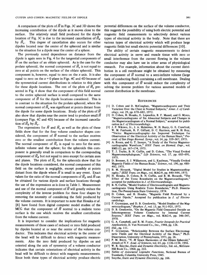
Fig. 3. Magnetic fields of dipoles in a prolate spheroid. For the spher-oid shown, C = 1.0 and na = 1.5. The scale is arbitrary but consistentfor all plots in this figure. Dipole locations (with apo = 0 for all cases)and the planes in which the fields are plotted are as follows: (B) to =

0.0, no = 1.15, z = 0; (C) to = 0.575, no = 1.0, y = 0; (D) to = 0.95,no= 1.0,y=0;(E) to=0.0,no= 1.15,x=0;and(F)to=0.5,no=1.15, x = 0.

where the prolate spheroidal variables are in the ranges -1It < 1, 1< 7, 0 < p < 2r and C is a constant. Therefore, Hdcan be calculated using equation (1).The evaluation of the surface integral in equation (4), which

gives Ha, requires an expression for the electric potential, V,produced on the surface of the spheroid (with rq = qa) by thevarious current dipoles. This expression can be adapted fromBerry [161 as

1 E (2 - 60)(21 + 1)(1 - k)! Pk'(t)4irC21 = ko- (i2 - 1)(l+k)!Pk0(f )

<[P1 Pa (no)Pf (to) cos k(sp - soo)

hto+Pno P' (no)Pt (to)cos k(sp - spo)

ho

+P~O Pk (110)Pk(to) k sin k(p - spo)+ h,0J(26)

(27)

with t = to, = ,o, and ,p = 'po. The following infinite seriesexpansion for the 1hR term which appears in the surfaceintegral can be obtained from Smythe: [ 17]

!=,C i, (a )(- m (2n + 1)(n )!]nC o m.do (n +rn)!J

X P(nW)Pn (Q)Qn ())Pn (pa) cos mr( P) (28)

where again the primed variables apply to the field point andthe unprimed apply to an element of surface. Equations (26),(27), and (28) can be substituted into the surface integral ofequation (4). In order to simplify the indicated integrations,the vector integrand is expressed in rectangular componentsand p = 0 is assumed. For a PtO dipole the integral becomes

i f v v jt. x rir

-V Xds= 4ChR 4raUC2hto

00, A (2 - 50)(21+ 1)(1- k)!Ppk)1=0 k=o (iIa 1 )(l + k)!Pl (71a)

X Pk (to)PkO(to) COS kso]

nX. (2 50 )(1)m (2n + 1)n=O m=o

X (n + m)!] PmTQ )Qn (l )PT (??a)X (72 1)1/2

{(-rn sin m(so' - op)t sin spPm Q)

(1 t2)1/2- (l -t2)1/)2 COS oPpm @(t) COS m (o' -_p)

(-im sin mr(so - sO)t cos epPT)(1 - 2)1/2

+( -a2 )1/2 sin spPm 0Q) cos m ( dp-c/p)

+ (na (2 1))/2n()]I dtdf

(29)

where , 5, and z are rectangular unit vectors.

A

Ei 41~ -%

x

z

C 0 .

4 . R

376

I

CUFFIN AND COHEN: MAGNETIC FIELDS OF DIPOLE

In order to evaluate equation (29), use is made of theorthogonality relationships between trigonometric functions.These require k = m ± 1 for the x and y components with m >O except for the second term of the i component where m >0. For the z component, the orthogonality relationshipsrequire k = m with m > 0. For all other combinations of kand m, integration with respect to ,p is equal to zero. Imposingthese limitations on k and m in the integration with respectto t, the following relationships can be developed. Consider-ing only the functions of t in the x component of equation(29) and with k = m - 1, integration with respect to t gives

I pmrn1 (t)[ ^Pn(t) - (1 - ta)1/2Pm()] dt

2(n + m)!

(2n+1)(n-im)!'=0, lIn. (30)

For k = m + 1, integration with respect to t gives

rPl + 2)1/2pn (0)] dt

P (I - t2)1/2

4HrC2(rj2 - 1)1/2( 2 - 2)1/2

X sin mnpP)())Qn(77)Pn(17a)

Prn+1(qo)Prn+1 t)]1

aP10(1 - o)1/2 n (2n+l)(- )m2irC2(i1a - 1)(o - to)1/2 nt-1 m<-i p~q®(71a)Xnsinin' Ln(n-r)! 2

X Pn(+m)Pn -t )P +tOfn (71)pnm(Qa Q (33

For a P~w0 dipole, the solution is the same as for the Odipole, except that the following substitutions must be madein equations (33):

2(n+m+ 1)!(2n + 1)(n - m - 1)! n

=0, lI=n. (31)

With appropriate change in sign, these same relations alsoapply to the y component in equation (29). For the z com-ponent, considering only the functions of t with k = mn,integration with respect to t gives

r = (n +n )!PI ( nP(~d (2n +1)(n -in)! '

=0, n. (32)

Using these relationships and recognizing the special case inthe x component when m = 0, the integral in equation (29)can be evaluated to give the following where the primes on thefield point coordinates have been dropped:

H Pto (1 -

V 47TC2(12 - 1)1/2(17r - o2)1/2

X0nt,, (2n + 1)( 1)(n m)!]1 2 ) -I

(n + in)!]

X CosM[(Pnn Q)Q nm((n )Pn (-a )

,(n + m)(n - m.+ I )PM -1 (??o)Pm -1O0

~ ~ ~ Mlpm~~+1@0

-0 (2n + 1)Pn'(fiO )Pn(to)Pn(t)Qn(fl)Pn(fla)}n-=1 Pnk(®Qla)

(1 - t2)1/2 = ( 2 - 1)1/2

Pm(TrO) = Pn'(fo)pmn (770 ) = Pn (70) (34)

The solution for a P9,0 dipole proceeds along the same linesand gives

PoHxV = ~4iC2(7 - 1)1/2(1 - t2)1/2(7l2 1)1/2

00 n

x£ (2n+1)(-1)mn=1 m=1

x [( j sin mpP' Q)Qm(7)Pn (tqa)

_(in +m)(m - l )(n + m)(n - m + I)Pm -(7n0)Pm-(Qo)

H = V~OYV4nC2 (fi - 1)1/2(1 - tO)1/2(r~a - 1)1/2

x , (+(in+ ~ ~ (7a

n=1 ~

X r(m-1)(+m)(P-M+ l)n1(770)Pnm -IS0

pn + n(

n =OaP (a

377

IEEE TRANSACTIONS ON BIOMEDICAL ENGINEERING, JULY 1977

Hz ??a P½ 00

2rrC2(712 - 1)(772 - 1)1/2(1 -2)1/2X0 n (2n + I)(- I)mE E PMe)n=1 m=l n "7qaJ

X [(n m)! m2

X cos mOp~n'(170)Pn (0 )Pn (t)Qn (q)Pnm (7)- (35S)

Equations (33), (34), and (35) provide means for calculatingH0 produced by the volume currents flowing in the. spheroidwhich are generated by PtO, P'70, and PP,0 current dipoles,respectively. In order to obtain H, Hd as calculated fromequation (1) must be added to these expressions. Some repre-sentative plots of H and Hv produced by various dipoles in aprolate spheroid are presented in Fig. 3. If to = 1 or no = 1,then the following relations must be used in order to performthe calculations:

(1 - SO)1/2pm®0(o --n(n + 1)

=0,

(-7 1)1/2pnO(nO) =n(n + 1)

=0,

m=1

me I

m =1

m= 1. (36)

For the plots in Fig. 3, the infinite series in the expressionsfor H0 are truncated for n greater than 10. The values of theassociated Legendre polynomials are calculated using therecurrence relationships and are in agreement with valuesavailable in standard tables [18]. Several tests of the ability ofthis number of terms to accurately represent the solution wereperformed. One test involves calculating the field for a dipolelocated at various points on the axis and pointing in the zdirection. Because of. the symmetry present for these condi-tions, the H should be equal to zero; therefore, Hd = -H,. Forthis test, H, is equal and opposite to Hd to within 0.2% in theWorst case for the points at which the field is calculated.Another test was performed by varying the maximum value ofn for a Pt, dipole located off the z axis (to = 0, 710 = 1.15).As expected, the differences between the series solutionsdecrease as the maximum value of n increases. For this test,the maximum difference between the solution for n = 9 andn = 10 is approximately 8%. These comparisons are made forthe field in the plane normal to the dipole and interestinglythe greatest difference occurs at the point which is farthestfrom the dipole, which is where H is smallest. Since theexpressions for H, are infinite series, no convenient expressionfor the ratios of the components of Hd and H can bedeveloped. These ratios can be calculated for particular loca-tions as required. As an example, these ratios for the normaland tangential components of the fields on the surface of thespheroid of Fig. 3F are presented in Table 1.

TABLE ICOMPARISON OF Hd/H RATIOS FOR NORMAL AND TANGENTIAL FIELD

COMPONENTS ON THE SURFACE OF A PROLATE SPHEROID

Field H1 nlocation (normal) Hd /H (tangential) H/H

1 0.05 1.00 -0.07 -3.15

2 0.11 1.62 -0.11 -2.07

3 0.18 1.50 -0.15 -1.85

4 0.42 1.27 -0.24 -2.00

5 0.84 1.12 -0.20 -5.10

6 1.21 1.03 0.44 5.977 -0. 83 1.12 0.83 4.02

8 -0.93 1.13 -0.01 -242. 71

9 -0.43 1.0 -0.14 -5. 75

Note: Ratios are calculated for the fields produced by the dipole asshown in Fig. 3F. Field locations are on the surface of the spheroidwith location 1 on negative z axis, location 5 on the positive y axis, -and.location 9 on the positive z axis. Note that for the x = 0 plane in Fig.3F,H =H<v=Hd = 0.

Oblate SpheroidFor the oblate spheroid the development proceeds in the

same manner as for the prolate spheroid. In the oblatespheroidal coordinate system presented in Fig. 4A

x =Q

y= C[(1 - 22)(l + P2)] 1/2 Cos $°

z = C[(1 - 02)(1 + ¢2)]1/2 sinpp (37)

where-l< 1; 0.<;0<p<27r,andCisaconstant. Themetric coefficients are

2 Z+ ~2 )1/2

ht =Ct+ )

ho =C[(l - 22 )(1 + 2 )] 1/2. (38)

Again Hd can be calculated using equation (1), the expres-sion for the electrical potential produced on the surface of theoblate spheroid (with ¢ = P) can be adapted from Berry [16],and 1IR in oblate spheroid coordinates can be expressed as aninfinite series [19]. Proceeding with the same generalmethods as those used for the prolate spheroid, expressions forH, for the oblate spheroid can be developed. In the followingexpressions, to and to refer to the location of the dipole(with Poo = 0), while t, ¢, and p refer to the field point. For aPRO dipole, the following expression for H, is developed:

- ~a~t(i - d2)1/28 aPC o(+ +.20)1/2Vx 8C2(l + ¢a2)(t20 + ¢2)1/2

oo n i (2n+ )(-1)m [(n-m)!n-L m-PM (an+ m)!

X m sin mspP' (ra)Qm (j )P n PM

378

CUFFIN AND COHEN: MAGNETIC FIELDS OF DIPOLE

C

4 -D t 4r o-

z z

y y

~ Pto(i - 0 )1/24TC2(I + 2)1/2 (t2 + 2)1/2

00 nX E E j (2n + 1)(- I)m

n=l m=l

~[~; ~;1P2 (& Q OmQ COS rn~pj(n+ )!]

(n + m ) (n - m + I )Pm - 1 (&jO)Pm -l0

PXn iGa(j)

Pn (&tO)PTn+

t16

1

v°° j(2n + 1 )P1(jto )Pn (to )Pn (ja)Qn (j¢)pn(t)n=-1 Pn ( aL)

(39)

For a PR0 dipole, equation (39) can be used after the follow-ing substitutions are made:

(I - t2)1/2 = (I + jo)1/2P~n (&jO) = PT 0( &;)

(40)F n (to ) =p tnme e i i)For a P,,O dipole, the expression is

F

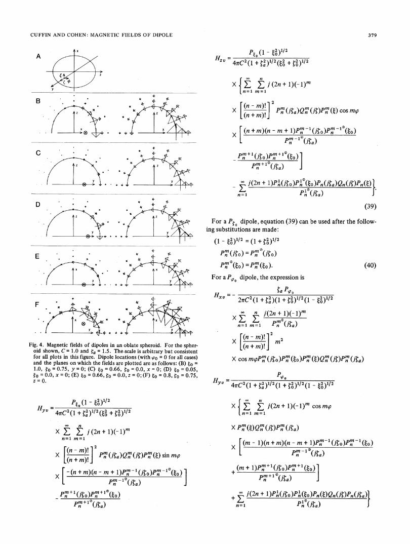
Fig. 4. Magnetic fields of dipoles in an oblate spheroid. For the spher-oid shown, C = 1.0 and ra = 1.5. The-scale is arbitrary but consistentfor all plots in this figure. Dipole locations (with V'o = 0 for all cases)and the planes on which the fields are plotted are as follows: (B) to =

1.0, to = 0.75, y = 0; (C) to = 0.66, *o = 0.0, x = 0; (D) to = 0.05,

o= 0.0, x = 0; (E) to= 0.66, =o0.0,z =0;(F)to=0.8, o = 0.75,z = 0.

Pt (1 o2)1/2Cy v + .2 )1/2 (t2 + t2 )1/2

00 n

X Z E i (2nt + 1)(- 1)mn=1 m=i

[( m)! Pmn(&~)Qm(jt)PmQt)sinm<,o[(n -rnm)! 12n

X [-(n + m)(n -m + l)P -1(i&o)Pm-1(t )

Pn(j~o )Pnn n Q)~ lO~ m-) (a)

pn 1cD+b.)

xv - 2irC2 (l + 2)(1 + t2)1/2 (I -t2)

X { m j(2n + 1)(-l)mn=l m=l+ nm

+(n - m)! 22.(n + mY!XcomOn~t)n (t)n ()n (})n /

HY 47rC2 (l + a2 )1/2 (1 + t2 )1/2 (1 - t2 )1/200~~ ~~n

X:£ j(2n + I)(- I)m cosmep.n=l m=l

X Pnm (Q)Qn ( O¢PT (ia)

x(m -l(n + m)(n - m + I)Pnm-' jO)PMn 1 Qo)

+(m + OPT (ItM)Pn (to )+

pm+o1 (i

oo j(2n + 1I)Pn(M9o )Pnlto )PnQ()Qn(j0Pn(ja)n-l Pn Mja)J

379

IEEE TRANSACTIONS ON BIOMEDICAL ENGINEERING, JULY 1977

PIH2V 47C2(1 + t,)l/2(1 + t2)l/2(1 t2)1/2

00 n

X Y. A (2n + 1)(- J)Mn=i m=1

X si n ~ ~ ~~ ~(n )! 2

X sin wfPn ()n (;)n Ia[n+m)]

Dim - 1)(n + m)(n - m + J)PnM -1 (&¢)pm -1 O)xL ~~~~PnM-lo )(jt((I(a)

(m n&PM (~O)

Rd H, given (39), (40), or (41),

H produced by various dipoles in the oblate spheroid can becalculated. Some representative plots of H and H. using a

maximum value of n = 10 are presented in Fig. 4. As is thecase with the prolate spheroid, the ratios of the components ofHd and H can be calculated for particular locations as

required.

DISCUSSION

These results provide a means to investigate and understandthe magnetic fields measured near the human body. Forexample, to a first approximation, the MCG may be con-

sidered to be produced by a dipole in a semi-infinite volumeand the MEG by a dipole in a sphere. Investigation of theeffect of changes in volume conductor shape can then proceedby comparing these fields with those produced by dipoles inprolate and oblate spheroids. The expressions for H are in a

convenient form to allow an investigation of the relative con-

tribution of Hd and his. The infinite series summations in Hafor the spheroids present no computational problems when a

digital computer is available.The plot of H in Fig. 1B shows that the components of this

field tangential to and on the surface of the semi-infinitevolume conductor are determined mainly by the dipole atpoints near the dipole, at distant points they are determinedmainly by the current flowing in the volume conductor near

that point. (Since Hz,, is equal to zero, the normal componentof H is determined completely by the dipole.) This resultseems reasonable since Hd is greatest directly over the dipoleand decreases as 1/R2 in moving away from it. Hence-, atdistant points the field should be determined mainly by thevolume current near that point. The change in direction of thefield with increasing distance along the x axis clearly showsthis change from a primarily dipole to a primarily volumecurrent field. Note that all components ofH are due solelyto the volume current. Comparison of all the plots ofH andH, in Fig. 1 shows that is generally in the direction oppo-site to Hd and therefore tends to cancel it. Recall that thefield lines of Hid are concentric circles lying in planes perpen-

dicular to the dipole, much like the field lines around an

infinitely long straight wire carrying a steady current. The factthat H2 , is equal to Zero accounts for the parallel field lines in

the plots ofH, in Figs. IC and ID.

For points on the surface of a sphere, the plot ofH in Fig.2B shows that the tangential components of this field aredetermined mainly by the dipole at points near the dipolewhile at distant points these componerits are determinedmainly by the volume current near that point. This is shown(in larger scale plots) by the field on the negative z axis, whichis in the direction opposite to that produced by the dipolealone. As is the case for the semi-infinite volume conductor,the component of H normal to the surface is due solely to thedipole. The plot ofH in Fig. 2C shows the influence of thelarge current loop flowing in the volume conductor. The plotof Ho in Fig. 2B shows that this field is in the directionopposite to Hd. For points near the dipole, H7 is less than Hdand therefore H is determined mainly by the dipole. Thereverse is true for points distant from the dipole. It should benoted that as the dipole is moved closer to the center of thesphere, H will decrease because of the increasing cancellationof Hd by H,. For a dipole at the center of a sphere, completecancellation of Hd by H, will occur. This may be viewed as aspecial case of the symmetry conditions for which H is equalto zero since any dipole at the center of a sphere will be aradial dipole. It should also be noted that since Hrv is equal tozero, the field lines of HII in Figs. 2B and 2C are tangential tothe surface of the sphere. This is similar to the parallel fieldlines of IJ, for the semi-infinite volume.Study of the plots ofH in Fig. 3 shows that the tangential

components of this field on the surface of a prolate spheroidhave the same dependence on distance from dipole location asthose for a sphere. Tangential components on the surface ofthe spheroid and near the dipole are determined mainly by thedipole, while those far from the dipole are determined mainlyby the volume current near that point. However, in contrastto the situation which exists for the sphere, the component ofHV normal to the surface of the prolate spheroid is not equalto zero over its entire surface. It can be seen from the geom-etry that the normal component of Hv is equal to zero on thez axis. It is also equal to zero on the z - 0 plane in Fig. 3Bbecause of the symmetrical distribution of current in relationto this plane for this particular dipole location.The plots of Fig. 3F show that the component ofHv normal

to the spheroid surface can become significant in comparisonto the same component ofH for points on the surface distancefrom the dipole. However, for points near the dipole, thiscomponent of H is determined mainly by the dipole. Thesame conclusions can be obtained from a study of the cal-culated ratios for the normal components of Hd and H pre-sented in Table 1. Note that the ideal value of this ratio is onewhich indicates that this component of both Hd and H areequal and pointing in the same direction. In addition, com-parison of the calculated ratios of the normal and tangentialcomponents ofHd andH shows that the normal component ofH receives the smallest contribution from H,. This is clearlyshown by the fact that the ratios for the normal componentare all positive and have a maximum magnitude of 1.62, whilethe ratios for the tangential components are negative for mostof the locations and have magnitudes greater than 2.00. Thenegative value of the ratio indicates that this component ofHdandH are in opposite directions.

380

CUFFIN AND COHEN: MAGNETIC FIELDS OF DIPOLE

A comparison of the plots ofH in Figs. 3C and 3D shows theincreasing contribution of the dipole as it moves close to thesurface. The relatively small field produced for the dipolelocation of Fig. 3C is due to the increased cancellation ofHdby H,. This degree of cancellation also occurs for otherdipoles located near the center of the spheroid and is similarto the situation for a dipole near the center of a sphere.The previously noted dependence on distance from the

dipole is again seen in Fig. 4 for the tangential components ofH on the surface of an oblate spheroid. As is the case for theprolate spheroid, the normal component of flU is not equal tozero at all points on the surface of the oblate spheroid. Thiscomponent is, however, equal to zero on the x axis. It is alsoequal to zero on the x = 0 plane in Figs. 4C and 4D because ofthe symmetrical current distributions in relation to this planefor these dipole locations. The rest of the plots of HR pre-sented in Fig. 4 show that the component of this field normalto the entire spheroid surface is small compared to the samecomponent of H for the dipole locations considered. This isin contrast to the situation for the prolate spheroid, where thenormal component of Hf was significant at points distant fromthe dipole for some dipole locations. Study of the plots ofHalso show that dipoles near the center tend to produce smallH(compare Figs. 4C and 4D) because of the increased cancella-tion ofHd by HfThe expressions for H and HU as well as the plots of these

fields show that for the four volume conductor shapes con-sidered, the component of H normal to the surface receiveszero or the smallest contribution from the volume current.The normal component of H, is equal to zero for the semi-infinite volume and the sphere; for the spheroids this com-ponent is generally small in comparison to the correspondingcomponent ofHd but not equal to zero except for certain axesand planes. The plots of Ha for the spheroids show that forthe dipole locations considered, the normal component of thisfield on the surface is negligible, except possibly at pointsdistant from the dipole where H is small in any event. Exactvalues for the ratio of the normal components ofHd and Hcanbe obtained for various dipole and surface locations throughthe use of the expressions as is done in Table 1. Measurementand use of the normal component ofH will greatly reduce thecomplexity of the inverse problem for these four shapes byremoving the necessity of considering the field produced bythe volume currents. It is important to note that Hosaka et al.[81 have found from digital computer model studies of theMCG that the component of H normal to a realistic torsosurface is the one which receives the smallest contributionfrom the volume current.

It is important to consider the implications for magneticmeasurements of those cases of reduced or zero field producedby dipoles located at or near the center of the volume con-ductor. This indicates that electrical activity in the center ofthe head will be difficult to detect with magnetic measure-ments. Also the zero field produced by dipoles on andoriented along the axis of symmetry of a volume conductorindicates that certain orientations of electrical activity in thehead will be difficult to detect with magnetic measurements.Since both these types of electrical activity produce electric

potential differences on the surface of the volume conductor,this suggests the possibility of using both electric potential andmagnetic field measurements to selectively detect varioustypes of electrical activity in the body. Note that there arevarious types of electrical activity which will produce largemagnetic fields but small electric potential differences [10].The ability of certain magnetic measurements to detect

electrical activity in nerve and muscle tissue with zero orsmall interference from the current flowing in the volumeconductor may also have use in other areas of physiologicalresearch. For example, information about the current distri-bution in a cell membrane might be obtained by measuringthe component of H7 normal to a semi-infinite volume (largetank of conducting fluid) containing a cell membrane. Dealingwith this component of H would reduce the complexity ofsolving the inverse problem for various assumed models ofcurrent distribution in the membrane.

REFERENCES[1] D. Cohen and D. McCaughan, "Magnetocardiograms and Their

Variation Over the Chest in Normal Subjects," Amer. J. of Cardi-ology, vol. 29, pp. 678-685, 1972.

[2] D. Cohen, H. Hosaka, E. Lepeschin, B. F. Massel, and G. Myers,"Magnetocardiograms of Six Abnormal Subjects and Changes inthe Magnetocardiogram of a Normal Subject," accepted for publi-cation in J. ofElectrocardiology.

[3] J. P. Wikswo, Jr., J. A. Malmivuo, W. H. Barry, G. E. Crawford,W. M. Fairbank, R. P. Giffard, D. C. Harrison, and R. H. Roy,"Vector Magnetocardiography-An Improved Technique forObservation of the Electrical Activity of the Human Heart," Pro-ceed. ofSan Diego Biomed. Symp., vol. 14, pp. 359-367, 1975.

[4] A. Rosen, and G. T. Inouye, "A Study of the Vector Magnetor-cardiographic Waveform," IEEE Trans. on Biomed. Engr., vol.BME-22, pp. 167-174, 1975.

[5] T. J. Teyler, B. N. Cuffin, and D. Cohen, "The Visual EvokedMagnetoencephalogram," Life Sciences, vol. 17, pp. 683-691,1975.

[6] D. Brenner, S. J. Williamson, and L. Kaufman, "Visually EvokedMagnetic Fields of the Human Brain," Science, vol. 190, pp. 480-482, 1975.

[7] B. M. Horacek, "Digital Model for Studies in Magnetocardiog-raphy," IEEE Trans. on Mags., voL MAG-9, pp. 440-444, 1973.

[8] H. Hosaka, D. Cohen, B. N. Cuffin, and B. M. Horacek, "TheEffect of the Torso Boundaries on the Magnetocardiogram,"accepted for publication in J. ofElectrocardiology.

[9] B. N. Cuffin, "Model Studies of Electrocardiograms and Magneto-cardiograms Using Realistic Torso Boundaries," Ph.D. Disserta-tion, The Pennsylvania State University, 1974.

[101 D. Cohen, and H. Hosaka, "Magnetic Field Produced by aCurrent Dipole," Accepted for publication in J. of Electro-cardiology.

[11] F. Grynszpan, and D. B. Geselowitz, "Model Studies of the Mag-netocardiogram," Biophys. J., vol. 13, pp. 911-925, 1973.

[121 D. B. Geselowitz, "On the Magnetic Field Generated Outside anInhomogeneous Volume Conductor by Internal CurrentSources," IEEE Trans. on Mags., vol. MAG-6, pp. 346-347,1970.

[13] G. A. Campbell, and R. M. Foster, Fourier Integrals for PracticalApplications, D. Van Nostrand Co., Inc., 1948, pg. 126.

[14] ibid., pg. 111.[15] F. Grynszpan, "Relationship Between the Surface Electromag-

netic Fields and the Electrical Activity of the Heart," Ph.D.Dissertation, University of Pennsylvania, 1971, pg. 26.

[16] P. M. Berry, "N, M Space Harmonics of the Oblate Spheroid,"Annals ofN. Y. Acad. of Sciences, vol. 65, pp. 1126-1134, 1956.

[17] W. R. Smythe, Static and Dynamic Electricity, 3rd. ed., McGraw-Hill Book Co., 1968, pg. 210.

[181 Tables of Associated Legendre Functions, National Bureau ofStandards, Columbia University Press, 1945.

[19] Smythe, Static and Dynamic Electricity, pg. 166.

381