Magnetic field control of near-field radiative heat transfer ... · Magnetic field control of near-field radiative heat transfer and the realization of highly tunable hyperbolic

PHYSICAL REVIEW B 92, 125418 (2015)

Magnetic field control of near-field radiative heat transfer and the realization of highly tunablehyperbolic thermal emitters

E. Moncada-Villa,1 V. Fernandez-Hurtado,2 F. J. Garcıa-Vidal,2 A. Garcıa-Martın,3 and J. C. Cuevas2,*

1Departamento de Fısica, Universidad del Valle, AA 25360, Cali, Colombia2Departamento de Fısica Teorica de la Materia Condensada and Condensed Matter Physics Center (IFIMAC),

Universidad Autonoma de Madrid, E-28049 Madrid, Spain3IMM-Instituto de Microelectronica de Madrid (CNM-CSIC), Isaac Newton 8, PTM, Tres Cantos, E-28760 Madrid, Spain

(Received 19 June 2015; published 14 September 2015)

We present a comprehensive theoretical study of the magnetic field dependence of the near-field radiative heattransfer (NFRHT) between two parallel plates. We show that when the plates are made of doped semiconductors,the near-field thermal radiation can be severely affected by the application of a static magnetic field. We find thatirrespective of its direction, the presence of a magnetic field reduces the radiative heat conductance, and dramaticreductions up to 700% can be found with fields of about 6 T at room temperature. We show that this strikingbehavior is due to the fact that the magnetic field radically changes the nature of the NFRHT. The field not onlyaffects the electromagnetic surface waves (both plasmons and phonon polaritons) that normally dominate thenear-field radiation in doped semiconductors, but it also induces hyperbolic modes that progressively dominatethe heat transfer as the field increases. In particular, we show that when the field is perpendicular to the plates,the semiconductors become ideal hyperbolic near-field emitters. More importantly, by changing the magneticfield, the system can be continuously tuned from a situation where the surface waves dominate the heat transferto a situation where hyperbolic modes completely govern the near-field thermal radiation. We show that this hightunability can be achieved with accessible magnetic fields and very common materials like n-doped InSb or Si.Our study paves the way for an active control of NFRHT and it opens the possibility to study unique hyperbolicthermal emitters without the need to resort to complicated metamaterials.

DOI: 10.1103/PhysRevB.92.125418 PACS number(s): 44.40.+a, 81.05.Xj, 78.20.Ls

I. INTRODUCTION

Radiative heat transfer is a topic with numerous funda-mental and technological implications across disciplines [1].Presently, the investigation of radiative heat transfer betweenclosely spaced objects is receiving great attention [2–6]. Thebasic challenges now are the understanding of the mechanismsgoverning thermal radiation at the nanoscale and the ability tocontrol this radiation for its use in novel applications. For along time, it was believed that the maximum radiative heattransfer between two objects was set by the Stefan-Boltzmannlaw for black bodies. However, this is only true when objectsare separated by distances larger than the thermal wavelength(9.6 μm at room temperature) and the radiative heat transferis dominated by propagating waves. When two objects arebrought in closer proximity, the thermal radiation is dominatedby interference effects and, more importantly, by the nearfield emerging from the materials surfaces in the form ofevanescent waves. This was first established theoretically byPolder and Van Hove in 1971 [7] using Rytov’s frameworkof fluctuational electrodynamics [8,9]. These researcherspredicted that the NFRHT could overcome the blackbody limitby several orders of magnitude, achieving what is referred toas super-Planckian thermal emission. Although this NFRHTenhancement was already hinted at in several experimentsin the late 1960s [10,11], its unambiguous confirmationcame only in recent years [12–27]. These experiments, inturn, have triggered off the hope that NFRHT may have animpact in different technologies such as heat-assisted magnetic

*[email protected]

recording [28,29], thermal lithography [30], scanning thermalmicroscopy [31–33], coherent thermal sources [34,35], near-field based thermal management [22,36–38], thermophoto-voltaics [39,40], and other energy conversion devices [41].

Presently, one of the central research lines in the fieldof radiative heat transfer is the search for materials wherethe NFRHT enhancement can be further increased. So far,the largest enhancements have been experimentally reportedin polar dielectrics [15,16,26], where the near-field thermalradiation is dominated by the excitation of surface phononpolaritons (SPhPs) [42]. Similar enhancements have beenpredicted and observed in doped semiconductors due to surfaceplasmon polaritons (SPPs) [23,27,43,44]. Recently, it hasbeen predicted that hyperbolic metamaterials could behaveas broadband super-Planckian thermal emitters [45–47]. Hy-perbolic metamaterials are a special class of highly anisotropicmedia that have hyperbolic dispersion. In particular, they areuniaxial materials for which one of the principal componentsof either the permittivity or the permeability tensors is oppositein sign to the other two principal components [48]. Hyperbolicmedia have been mainly realized by means of hybrid metal-dielectric superlattices and metallic nanowires embedded ina dielectric host [49,50]. It has been demonstrated that thesemetamaterials exhibit exotic optical properties such as negativerefraction, subwavelength imaging, and focusing, and theycan be used to do density of states engineering [49,50].In the context of radiative heat transfer, what makes thesemetamaterials so special is the fact that they can supportelectromagnetic modes that are evanescent in a vacuum gap,but they are propagating inside the material. This leads toa broadband enhancement of transmission efficiency of theevanescent modes [46]. This special property has motivated a

1098-0121/2015/92(12)/125418(18) 125418-1 ©2015 American Physical Society

http://dx.doi.org/10.1103/PhysRevB.92.125418

E. MONCADA-VILLA et al. PHYSICAL REVIEW B 92, 125418 (2015)

lot of theoretical work on the use of hyperbolic metamaterialsfor NFRHT [51–61]. However, no experimental investigationof this issue has been reported so far, which is mainly dueto the difficulties in handling these metamaterials. In thissense, it would be highly desirable to find much simplerrealizations of hyperbolic thermal emitters and, ideally, withtunable properties.

Another key issue in the field of radiative heat transfer isthe active control and modulation of NFRHT. In this respect,several proposals have been put forward recently. One of thethem is based on the use of phase-change materials [62,63],where the change of phase leads to a significant change inthe material dielectric function. These materials include analloy called AIST, where the phase change can be induced byapplying an electric field [63], and VO2, which undergoes ametal-insulator transition as a function of temperature [62].It has also been suggested that the NFRHT between chiralmaterials with magnetoelectric coupling can be tuned byultrafast optical pulses [64]. Another proposal to tune theNFRHT is to use ferroelectric materials under an externalelectric field [65], although the predicted changes are rathermodest (<17%). Let us also mention that very recently it hasbeen proposed that the heat flux between two semiconductorscan be controlled by regulating the chemical potential ofphotons by means of an external bias [66]. So, in short,although these proposals are certainly interesting, some ofthem are not easy to implement and others are either not veryefficient or they are restricted to very specific materials. In thissense, the challenge remains to introduce strategies to activelycontrol NFRHT in an easy and relatively universal way.

In this work we tackle and resolve some of the openproblems described above by presenting an extensive theo-retical analysis of the influence of an external dc magneticfield in the radiative heat transfer between two parallel platesmade of a variety of materials. We show that an appliedmagnetic field can indeed largely affect the NFRHT in abroad class of materials, namely doped (polar and nonpolar)semiconductors. We find that, irrespective of its orientation,the magnetic field reduces the NFRHT with respect to thezero-field case and we show that the reduction can be as largeas 700% for fields of about 6 T at room temperature. Thiseffect originates from the fact that the magnetic field not onlystrongly modifies the surface waves that dominate the NFRHTin doped semiconductors (both SPhPs and SPPs), but it alsogenerates broadband hyperbolic modes that tend to governthe heat transfer as the field is increased. In particular, whenthe applied field is perpendicular to the plates’ surfaces, thesemiconductors behave as hyperbolic thermal emitters withhighly tunable properties. By changing the field magnitudeone can continuously tune the system and realize situationswhere (i) surface waves dominate the NFRHT, (ii) both surfacewaves and hyperbolic modes contribute significantly to thenear-field thermal radiation, and (iii) only hyperbolic modescontribute to the NFRHT and surface waves cease to exist.On the other hand, when the field is parallel to the surfacesthe NFRHT is nonmonotonic as a function of the magneticfield. For moderate fields, surface waves and hyperbolic modescoexist, while for high fields the NFRHT is largely dominatedby hyperbolic modes. We emphasize that all these strikingpredictions are amenable to measurements and do not require

the use of any complicated metamaterial. Thus our work offersa simple strategy to actively control NFRHT in a broad varietyof materials and it also provides a very appealing recipeto realize near-field hyperbolic thermal emitters with highlytunable properties.

The remainder of this paper is structured as follows.Section II describes the system under study and the generalformalism for the description of NFRHT in the presence ofa magnetic field. We then turn in Sec. III to the applicationof the general results to the case of n-doped InSb as anexample of a polar semiconductor. We discuss in this sectionboth the results for different magnetic field orientations andthe realization of highly tunable hyperbolic thermal emitters.Section IV is devoted to the case of Si as an example ofnonpolar semiconductor. Section V summarizes our mainresults and discusses future directions. Finally, four appendixescontain the technical details of the general formalism and someadditional calculations that support the claims in this paper.

II. RADIATIVE HEAT TRANSFER IN THE PRESENCEOF A MAGNETIC FIELD: GENERAL FORMALISM

Our main goal is to compute the radiative heat transfer in thepresence of an external dc magnetic field within the frameworkof fluctuational electrodynamics [8,9]. For simplicity, we shallconcentrate here in the heat exchanged between two infiniteparallel plates made of arbitrary nonmagnetic materials andthat are separated by a vacuum gap of width d; see Fig. 1(a).The magnetic field can point in any direction and, followingFig. 1(a), we shall refer to the left plate as medium 1, thevacuum gap as medium 2, and the right plate as medium 3.

When a magnetic field is applied to any object, it results inan optical anisotropy that can be described by the followinggeneral permittivity tensor [67]:

ε =

⎛⎜⎝

εxx εxy εxz

εyx εyy εyz

εzx εzy εzz

⎞⎟⎠, (1)

where, according to Fig. 1(a), x and y lie in the interface planesand z corresponds to the surface normal. The componentsof the permittivity tensor depend on the applied magneticfield, as we shall specify below, and on the frequency (localapproximation). Let us recall that the off-diagonal elements inEq. (1) are responsible for all the well-known magneto-opticaleffects (Faraday effect, Kerr effects, etc.) [67]. Thus ourproblem is to compute the radiative heat transfer betweentwo anisotropic parallel plates. This generic problem has beenaddressed by Biehs et al. [68] and we just recall here the centralresult. The net power per unit of area exchanged betweenthe parallel plates is given by the following Landauer-likeexpression [68]:

Q =∫ ∞

0

dω

2π[�1(ω) − �3(ω)]

∫dk

(2π )2τ (ω,k,d), (2)

where �i(ω) = �ω/[exp(�ω/kBTi) − 1], Ti is the absolutetemperature of the layer i, ω is the radiation frequency,k = (kx,ky) is the wave vector parallel to the surface planes,and τ (ω,k,d) is the total transmission probability of theelectromagnetic waves. Notice that the second integral in

125418-2

MAGNETIC FIELD CONTROL OF NEAR-FIELD . . . PHYSICAL REVIEW B 92, 125418 (2015)

100 101 102 103 104 10510-1100101102

103104105106

Wavelength (μm)

d

(c)

Gap size (nm)

Hea

ttra

nsfe

rcoe

ffic

ient

(W/m

2 K)

(b)Totals-propagating modess-evanescent modesp-propagating modesp-evanescent modes

(a)d

1011 1012 1013 101410-1610-1510-1410-1310-1210-1110-1010-910-8

(2)

Spec

tralh

eatf

lux

(J/ra

dm

2 Κ)

ω (rad/s)

d = 10 nmd = 100 nmd = 1 μm

(1) (3)

T1 T3x

y z

104 103 102 101

FIG. 1. (Color online) (a) Schematic representation of the systemunder study: two parallel plates at temperatures T1 and T3 separatedby a vacuum gap of width d . (b) Heat transfer coefficient of n-dopedInSb as a function of the gap at zero magnetic field. We show the totalresult and the individual contributions of s- and p-polarized waves(both propagating and evanescent). (c) The corresponding zero-fieldspectral heat flux as a function of frequency (and wavelength) forthree different gaps.

Eq. (2) is carried out over all possible directions of k andit includes the contribution of both propagating waves withk < ω/c and evanescent waves with k > ω/c, where k is themagnitude of k and c is the velocity of light in vacuum. Thetransmission coefficient τ (ω,k,d) can be expressed as [68]

τ (ω,k,d)

={

Tr{[1 − R21R†21]D†[1 − R†

23R23]D}, k < ω/c,

Tr{[R21 − R†21]D†[R†

23 − R23]D}e−2|q2|d , k > ω/c,

(3)

where q2 =√

ω2/c2 − k2 is the z component of the wavevector in the vacuum gap and the 2 × 2 matrices Rij are thereflections matrices characterizing the two interfaces. Thesematrices have the following generic structure:

Rij =(

rs,sij r

s,p

ij

rp,s

ij rp,p

ij

), (4)

where rα,β

ij with α,β = s,p is the reflection amplitude forthe scattering of an incoming α-polarized plane wave intoan outgoing β-polarized wave. Finally, the 2 × 2 matrix Dappearing in Eq. (3) is defined as

D = [1 − R21R23e2iq2d ]−1. (5)

Notice that this matrix describes the usual Fabry-Perot-likedenominator resulting from the multiple scattering betweenthe two interfaces.

In Appendixes A and B we provide an alternative derivationof the central result of Eq. (3) that emphasizes the nonre-ciprocal nature of our problem. More importantly, we showexplicitly how the different reflection matrices appearing inEq. (3) can be computed within a scattering-matrix approachfor anisotropic multilayer systems. This approach provides, inturn, a natural framework to analyze different issues that willbe crucial later on such as the nature of the electromagneticmodes responsible for the heat transfer.

The result of Eqs. (2) and (3) reduces to the well-knownresult for isotropic media first derived by Polder and VanHove [7]. In that case, the reflections matrices of Eq. (4) arediagonal and the nonvanishing elements are given by

rs,sij = qi − qj

qi + qj

, (6)

rp,p

ij = εjqi − εiqj

εjqi + εiqj

, (7)

where qi =√

εiω2/c2 − k2 is the transverse or z componentof the wave vector in layer i and εi(ω) is the corresponding di-electric constant. Thus the total transmission can be written asτ (ω,k,d) = τs(ω,k,d) + τp(ω,k,d), where the contributionsof s- and p-polarized waves are given by

τα=s,p(ω,k,d)

={

(1 − |rα,α21 |2)(1 − |rα,α

23 |2)/|Dα|2, k < ω/c,

4 Im{rα,α21 }Im{rα,α

23 }e−2|q2|d/|Dα|2, k > ω/c,(8)

where Dα = 1 − rα,α21 r

α,α23 e2iq2d . Throughout this work we

focus on the analysis of the radiative linear heat conductanceper unit of area, h, which is referred to as the heat transfercoefficient. This coefficient is given by

h(T ,d) = limT →0+

Q(T1 = T + T,T3 = T ,d)

T, (9)

where T is the absolute temperature that we assume equalto 300 K throughout this work. Additionally, we define thespectral heat flux as the heat transfer coefficient per unit offrequency. In the following sections, we apply the generalresults presented here to different materials and magnetic fieldconfigurations.

III. POLAR SEMICONDUCTORS: InSb

The first obvious question to be answered is the following:in which materials can a magnetic field modify the NFRHT?Since the thermal radiation of an object is primarily determinedby its dielectric function, we need materials in which thisfunction can be modified by an external magnetic field,that is we need magneto-optical (MO) materials. Focusing

125418-3


on room temperature experiments, the MO activity must beexhibited in the midinfrared. Thus doped semiconductors,where the MO activity is due to conduction electrons, areideal candidates [69]. In these materials, one can play withthe doping level to tune the plasma frequency to valuescomparable to the cyclotron frequency at experimentallyachievable magnetic fields, which is an important requirementto have sizable magnetic-induced effects in the NFRHT (seediscussion below). Moreover, in semiconductors the NFRHTin the absence of field is typically dominated by surfaceelectromagnetic waves (both SPhPs and SPPs), which in turnare known to be strongly influenced by an external magneticfield [69,70]. Thus it seems natural to expect a magnetic fieldmodulation of NFRHT in semiconductors.

There is a variety of semiconductors that we could chooseto illustrate our predictions. In this section we focus on InSbfor several reasons. First, it is a polar semiconductor where theNFRHT in the absence of field is dominated by two differenttypes of surface waves (SPhPs and SPPs), which allows usto study a very rich phenomenology. Second, InSb has asmall effective mass, which enables one to tune the cyclotronfrequency to values comparable to those of the plasmafrequency with moderate fields. Finally, InSb has been the mostwidely studied material in the context of magnetoplasmons andcoupled magnetoplasmons-surface phonon polaritons. Thusthe magnetic field effect in the surface waves has been verywell characterized experimentally [71–74].

A. Perpendicular magnetic field: The realization of hyperbolicnear-field thermal emitters

Let us first discuss the radiative heat transfer between twoidentical plates made of n-doped InSb when the magneticfield is perpendicular to the plate surfaces, i.e., H = Hzz; seeFig. 1(a). In this case, the permittivity tensor of InSb adoptsthe following form [73]:

ε(H ) =

⎛⎜⎝

ε1(H ) −iε2(H ) 0

iε2(H ) ε1(H ) 0

0 0 ε3

⎞⎟⎠, (10)

where

ε1(H ) = ε∞

(1 + ω2

L − ω2T

ω2T − ω2 − iω

+ ω2p(ω + iγ )

ω[ω2

c − (ω + iγ )2])

,

ε2(H ) = ε∞ω2pωc

ω[(ω + iγ )2 − ω2

c

] , (11)

ε3 = ε∞

(1 + ω2

L − ω2T

ω2T − ω2 − iω

− ω2p

ω(ω + iγ )

).

Here, ε∞ is the high-frequency dielectric constant, ωL isthe longitudinal optical phonon frequency, ωT is the trans-verse optical phonon frequency, ω2

p = ne2/(m∗ε0ε∞) definesthe plasma frequency of free carriers of density n and effectivemass m∗, is the phonon damping constant, and γ is thefree-carrier damping constant. Finally, the magnetic fieldenters in these expressions via the cyclotron frequency ωc =eH/m∗. The important features of the previous expressionsare as follows: (i) the magnetic field induces an optical

anisotropy (via the modification of the diagonal elementsand the introduction of off-diagonal ones), (ii) there aretwo major contributions to the diagonal components of thedielectric tensor: optical phonons and free carriers, and (iii)the MO activity is introduced via the free carriers, whichillustrates the need to deal with doped semiconductors. Inwhat follows we shall concentrate in a particular case takenfrom Ref. [73], where ε∞ = 15.7, ωL = 3.62 × 1013 rad/s,ωT = 3.39 × 1013 rad/s, = 5.65 × 1011 rad/s, γ = 3.39 ×1012 rad/s, n = 1.07 × 1017 cm−3, m∗/m = 0.022, and ωp =3.14 × 1013 rad/s. As a reference, let us say that with theseparameters ωc = 8.02 × 1012 rad/s for a field of 1 T. Let uspoint out that in this configuration, and due to the structure ofthe permittivity tensor, the transmission coefficient appearingin Eq. (2) only depends on the magnitude of the parallel wavevector, which considerably simplifies the calculation of theradiative heat transfer.

Let us now briefly review the expectations for the heattransfer in the absence of magnetic field. As we show inFig. 1(b), the heat transfer coefficient features a large near-fieldenhancement for gaps below 1 μm. For d < 100 nm thisenhancement is largely dominated by p-polarized evanescentwaves and the heat transfer coefficient increases as 1/d2

as the gap decreases, which are two clear signatures of asituation where the heat transfer is dominated by surfaceelectromagnetic waves. This can be further confirmed withthe analysis of the spectral heat flux, see Fig. 1(c), which inthe near-field regime is dominated by two narrow peaks thatcan be associated to SPPs (low-frequency peak) and SPhPs(high-frequency peak), as it will become evident below. Thusthe case of InSb constitutes an interesting example where twotypes of surface waves contribute significantly to the NFRHT.Let us now see how these results are modified in the presenceof a magnetic field.

In Fig. 2(a) we show the heat transfer coefficient as afunction of the gap size for different values of the perpendicularmagnetic field. There are three salient features: (i) the far-fieldheat transfer is fairly independent of the magnetic field, (ii)in the near-field regime (below 300 nm) the magnetic fieldsuppresses the heat transfer by up to a factor of 3 (see inset),and (iii) by increasing the field, the heat transfer coefficienttends to saturate at around 6 T, although it is slightly reducedupon further increasing the field above 10 T (not shown here).The strong modification of heat transfer due to the magneticfield is even more apparent in the spectral heat flux. As one cansee in Fig. 2(b), the magnetic field not only distorts and reducesthe height of the peaks related to the surface waves, but it alsogenerates a new peak that shifts to higher frequencies as thefield increases. This additional peak appears at the cyclotronfrequency and its presence illustrates the high tunability thatcan be achieved. Notice, for instance, that for a field of 6 T thethermal emission at the cyclotron frequency is increased byalmost three orders of magnitude with respect to the zero-fieldcase.

To shed more light on these results it is convenient toexamine the transmission of the p-polarized waves, which canbe shown to dominate the heat transfer for any field. We presentin Fig. 3 this transmission as a function of the magnitude of theparallel wave vector, k, and the frequency for a gap d = 10 nmand different values of the magnetic field. As one can see,

125418-4


100 101 102 103 104 105100

101

102

103

104

105

106

Wavelength (μm)

(b)

Gap size (nm)

Hea

ttra

nsfe

rcoe

ffic

ient

(W/m

2 K)

(a)

Hz = 0 THz = 2 THz = 4 THz = 6 THz = 8 T

Hz = 0 THz = 2 THz = 6 T

Hz = 10 T

1013 101410-14

10-13

10-12

10-11

10-10

10-9

10-8

Spec

tralh

eatf

lux

(J/ra

dm

2 K)

ω (rad/s)

Hz = 8 T

100 101 102 103

1.0

1.5

2.0

2.5

3.0

h(0

)/h

(Hz)

Gap size (nm)

102×2 102 2 101×

FIG. 2. (Color online) (a) Heat transfer coefficient for n-dopedInSb as a function of the gap for different values of the magnetic fieldperpendicular to the plate surfaces. The inset shows the ratio betweenthe zero-field coefficient and the coefficient for different values ofthe field in the near-field region. (b) The corresponding spectral heatflux as a function of the frequency (and wavelength) for a gap ofd = 10 nm and different values of the perpendicular field. The solidlines correspond to the exact calculation and the circles to the uniaxialapproximation where the off-diagonal terms of the permittivity tensorare assumed to be zero.

at low fields the transmission maxima are located arounda restricted area of k and ω, clearly indicating that surfacewaves dominate the NFRHT. Notice also that their dispersionrelation is modified by the field; see Fig. 3(b). By increasing thefield, those areas are progressively replaced by areas where themaximum transmission is reached for a broad range of k valuesand, finally, the surface waves are restricted to the reststrahlenband ωT < ω < ωL for the highest fields; see Fig. 3(d). Whatis the nature of these magnetic field induced modes?

To answer this question and explain all the results justdescribed, it is important to realize that the off-diagonalelements of the permittivity tensor do not play a major rolein this configuration. This is illustrated in Fig. 2(b) where weshow that the approximation consisting in setting ε2 = 0 inEq. (10) reproduces very accurately the exact results for thespectral heat flux for arbitrary magnetic fields. This meansthat the polarization conversion is irrelevant and the plateseffectively behave as uniaxial media where their permittivitytensors are diagonal: ε = diag[εxx,εxx,εzz], where εxx = ε1

and εzz = ε3. Within this approximation, which hereafter we

refer to as uniaxial approximation, it is easy to compute thedispersion relation of the surface electromagnetic modes in ourgeometry (see Appendix D). In the electrostatic limit k � ω/c,the dispersion relation of these cavity modes is given by

kSW = 1

dln

(±εxx − √

εxx/εzz

εxx + √εxx/εzz

), (12)

with the additional constraint that both εxx and εzz mustbe negative. In the zero-field limit, this expression reducesto the known result for cavity surface modes in isotropicmaterials [26]. As we show in Fig. 3, see white solid lines, thedispersion relation of Eq. (12) nicely reproduces the structureof the transmission maxima in those frequency regions inwhich surfaces waves are allowed (εxx,εzz < 0). It is worthstressing that this dispersion relation describes in a unifiedmanner both the SPPs that appear below the reststrahlen bandand the SPhPs due to the optical phonons. More importantly,this dispersion relation tells us that the magnetic field reducesthe magnitude of the parallel wave vector of the surface waves,which is one of one the causes for the reduction of the NFRHT.Moreover, the analysis of Eq. (12) tells us that the magneticfield also restricts the frequency region where the surfacewaves exist. Indeed, at high fields the SPPs disappear, whilethe SPhPs are restricted to the reststrahlen band, Fig. 3(d).These two effects are actually the cause of the reduction of theNFRHT in the presence of a magnetic field. But what about theother modes that appear by increasing the field? Their naturecan also be understood within the uniaxial approximation. Aswe show in Appendix C, the allowed values for the transversecomponent of the wave vector inside these uniaxial materialsare given by qo =

√εxxω2/c2 − k2 for ordinary waves and

qe =√

εxxω2/c2 − k2εxx/εzz for extraordinary waves. Thedispersion of the extraordinary waves can be rewritten as

k2x + k2

y

εzz

+ q2e

εxx

= ω2

c2, (13)

a dispersion that becomes hyperbolic when εxx and εzz haveopposite signs [48]. This is exactly what happens in our casein certain frequency regions at finite field. This illustratedin Figs. 3(b)–3(d), where we have indicated the hyperbolicregions defined by the condition εxxεzz < 0. Notice that thoseregions correspond exactly to the areas where the transmissionreaches its maximum for a broad range of k values. This factshows unambiguously that our InSb plates effectively behaveas hyperbolic materials. More importantly, and as it is evidentfrom Fig. 3, we can easily modify the hyperbolic regionsby changing the field. Thus we can change from situationswhere the hyperbolic modes (HMs) coexist with both typesof surface waves to situations where the HMs dominate theNFRHT, which is what occurs at high fields; see Fig. 3(d).Moreover, contrary to what happens in most hybrid hyperbolicmetamaterials, we can have in a single material HMs of type I(HMI), where εxx > 0 and εzz < 0, and HMs of type II (HMII),where εxx < 0 and εzz > 0; see Figs. 3(b)–3(d).

Let us recall that what makes HMs so special in thecontext of NFRHT is the fact that, as it is evident from theirdispersion relation, they are evanescent in the vacuum gapand propagating inside the hyperbolic material for k > ω/c

(HMI) or k >√|εzz|ω/c (HMII). Thus they are a special

125418-5


FIG. 3. (Color online) Transmission coefficient for p-polarized waves as a function of the magnitude of the parallel wave vector andfrequency for InSb and a gap of d = 10 nm. The different panels correspond to different values of the magnetic field that is perpendicular to thesurfaces. The horizontal dashed lines separate the regions where transmission is dominated by surface waves (SPPs and SPhPs) or hyperbolicmodes of type I and II (HMI and HMII). The white solid lines correspond to the analytical dispersion relation of the surface waves of Eq. (12).

kind of frustrated internal reflection modes that exhibit avery high transmission over a broad range of k values thatcorrespond to evanescent waves in the vacuum gap [46]. Asshown in Ref. [46], the number of HMs that contributes tothe NFRHT is solely determined by the intrinsic cutoff inthe transmission, which has the form τ (ω,k) ∝ exp(−2kd) fork � ω/c. From this condition it follows that the heat flux dueto HMs scales as 1/d2 for small gaps, as the contribution ofsurface waves. This explains why the appearance of HMs as thefield increases does not modify the parametric dependence ofthe NFRHT with the gap size. Notice, however, that in spite ofthe high transmission of these HMs, their appearance does notenhance the NFRHT because their wave vector cutoffs (beyondwhich they give a negligible contribution) are clearly smallerthan the k values of the surface waves that they replace (noticethat the conditions of HMs and surface waves are mutuallyexcluding). Thus we can conclude that the NFRHT reductioninduced by the magnetic field is due to both the modification ofthe surface waves and their replacement by HMs that, in spiteof their propagating nature inside the material, turn out to beless efficient transferring the radiative heat in the near-fieldregion than the surface waves.

Let us point out that within the uniaxial approximation,the heat transfer can be obtained in a semianalytical form. Inthis case, the transmission coefficient is given by the isotropicresult of Eq. (8), where the reflections coefficients adopt nowthe form

rs,s21 = r

s,s23 = q2 − qo

q2 + qo, (14)

rp,p

21 = rp,p

23 = εxxq2 − qe

εxxq2 + qe. (15)

The uniaxial approximation is also useful to understand thehigh field behavior of the NFRHT. The tendency to saturatethe thermal radiation as the field increases is due to the factthat the cyclotron frequency becomes larger than the plasmafrequency and the last term in the expression of εxx = ε1,see Eq. (11), progressively becomes more irrelevant. Thus thepermittivity tensor becomes field independent and the heattransfer is simply given by the result for uniaxial media, whereεzz = ε3 has the form in Eq. (11), but εxx = ε1 does not containthe last term in the first expression of Eq. (11). We find that the

strict saturation of the NFRHT occurs at around 20 T and thereis an intermediate regime, between 6 and 20 T, in which thenear-field thermal radiation slightly increases upon increasingthe field (not shown here), leading to a nonmonotonic behavior.This behavior is due to an increase in the efficiency of the HMsthat dominate the NFRHT in this high-field regime.

To conclude this subsection, let us explain why the far-fieldheat transfer is rather insensitive to the magnetic field. Forgaps much larger than the thermal wavelength (9.6 μm), theheat transfer is dominated by propagating waves and, as weshow in Fig. 4, the spectral heat flux in the absence of fieldexhibits a broad spectrum with a peak at around 1.5 × 1014

rad/s. Indeed, the spectrum is very similar to that of a dielectricwith a frequency-independent dielectric constant ε = ε∞1; seedotted line in Fig. 4. As we illustrate in that figure, the presenceof a magnetic field only modifies this spectrum in a significantway in a small region around the cyclotron frequency. Thisfact leads to a tiny modification of the heat transfer upon the

1 2 3 40.0

0.5

1.0

1.5

Wavelength (μm)

Spec

tralh

eatf

lux

(10−1

4J/

rad

m2 Κ

)

ω (1014 rad/s)

18.8 9.4 6.3 4.7

Hz = 0 THz = 4 THz = 8 THz = 12 THz = 16 THz = 20 T

1 3 ∞= =

4 6 8 10 12 14 16 181.0001.0051.0101.0151.0201.025

h(0

)/h

(Hz)

Hz (T)

FIG. 4. (Color online) Far-field spectral heat flux for InSb as afunction of the frequency (and wavelength) for different values ofthe perpendicular field. These spectra have been computed for a gapd = 1 m. The dotted line corresponds to the result for plates made ofa dielectric with a frequency-independent dielectric constant equal toε∞. The inset shows the corresponding ratio between the zero-fieldheat transfer coefficient and the coefficient for different values of thefield.

125418-6


application of an external field. As it can be seen in the insetof Fig. 4, the magnetic field reduces the far-field heat transfercoefficient as the magnetic field increases, but this reductionis quite modest and, for instance, it amounts to only 2.5% at avery high field of 20 T.

B. Parallel magnetic field

Let us now turn to the case in which the magnetic field isparallel to the plate surfaces. For concreteness, we consider thatthe field is applied along the x axis, H = Hx x, but obviouslythe result is independent of the field direction as long as itpoints along the surface plane, as we have explicitly checked.In this case, the permittivity tensor of InSb adopts the form

ε(H ) =

⎛⎜⎝

ε3 0 0

0 ε1(H ) −iε2

0 iε2(H ) ε1(H )

⎞⎟⎠, (16)

where the ε’s are given by Eq. (11). Let us emphasize thatin this case the transmission coefficient appearing in Eq. (2)depends both on the magnitude of the parallel wave and on itsdirection, which makes the calculations more demanding. Letus also say that we consider here the same parameter valuesfor the n-doped InSb as in the example analyzed above.

The results for the magnetic field dependence of theheat transfer coefficient for the parallel configuration aresummarized in Fig. 5(a). As in the perpendicular case, thefar field is barely affected by the magnetic field, the near-fieldthermal radiation is suppressed by the field, and at high fieldsthe NFRHT tends to saturates. Interestingly, it saturates to thesame value as in the perpendicular configuration. In spite of thesimilarities, there are also important differences. In this case,the NFRHT is much more sensitive to the field and a significantreduction is already achieved at 1 T. Notice also that in thiscase the heat transfer coefficient is clearly nonmonotonic andthe maximum reduction is reached at around 6 T. Finally,notice also that the reduction is more pronounced than in theperpendicular case and the NFRHT can be diminished by upto a factor of 7 with respect to the zero-field case; see insetof Fig. 5(a). This more pronounced reduction in the parallelconfiguration is also apparent in the spectral heat flux, as onecan see in Fig. 5(b). Notice that also in this case there appearsa high-frequency peak that is blueshifted as the field increases.This peak appears at the cyclotron frequency and it has thesame origin as in the perpendicular case.

Again, to understand this complex phenomenology, it isconvenient to examine the transmission of the p-polarizedwaves, which dominate the NFRHT for any field. Since in thiscase the transmission also depends on the direction of k, wechoose to analyze the two most representative directions. Inthe first one, the in-plane wave vector k is parallel to the field,i.e., k = (kx,0), and in the second one, k is perpendicular tothe field, i.e., k = (0,ky). The transmission of p-polarizedwaves for these two directions is shown in Fig. 6 as a functionof the magnitude of the wave vector and as a function of thefrequency for different values of the field. As one can see, thetransmission exhibits very different behaviors for these twodirections. While for k ‖ H the situation resembles that of aperpendicular field (see discussion above), for k ⊥ H it seems

100 101 102 103 104 105100

101

102

103

104

105

106

Gap size (nm)

h(0

)/h

(Hx)

(b)

(a)

Hea

ttra

nsfe

rcoe

ffic

ient

(W/m

2 K)

Gap size (nm)

Hx = 0 THx = 1 THx = 2 THx = 6 T

Hx = 8 THx = 12 T

1013 101410-14

10-13

10-12

10-11

10-10

10-9

10-8

Spec

tralh

eatf

lux

(J/ra

dm

2 K)

ω (rad/s)

Hx = 0 THx = 1 THx = 2 THx = 6 T

Hx = 8 THx = 12 T

102× ×2 102 2 101

Wavelength (μm)

100 101 102 103

1234567

FIG. 5. (Color online) (a) Heat transfer coefficient for n-dopedInSb as a function of the gap for different values of the magnetic fieldapplied along the surfaces of the plates. The inset shows the ratiobetween the zero-field coefficient and the coefficient for differentvalues of the field in the near-field region. (b) The correspondingspectral heat flux as a function of the frequency (and wavelength) fora gap of d = 10 nm and different values of the parallel field.

like the transmission is dominated by surface waves that areseverely affected by the magnetic field (with the appearanceof gaps in their dispersion relations). These very differentbehaviors can be understood with an analysis of both thesurface waves and the propagating waves inside the materialin these two situations. In the case k ‖ H, one can show thata uniaxial approximation, similar to that discussed above,accurately reproduces the results for the transmission found inthe exact calculation. In this case, the permittivity tensor canbe approximated by ε = diag[εxx,εzz,εzz], where εxx = ε3

and εzz = ε1. Within this approximation, the dispersionrelation of surface waves in the electrostatic limit k � ω/c

is also given by Eq. (12) (see Appendix D). As we show inFigs. 6(a)–6(c), this dispersion relation nicely describes thestructure of the transmission maxima in the regions where thesurface waves can exist (εxx,εzz < 0). On the other hand, aswe show in Appendix C, the allowed values for the transversecomponent of the wave vector inside these uniaxial-likematerials are given by qo =

√εzzω2/c2 − k2 for ordinary

waves and qe =√

εxxω2/c2 − k2εxx/εzz for extraordinarywaves. Again, the dispersion of these extraordinary wavesis of hyperbolic type when εxx and εzz have opposite signs.In Figs. 6(a)–6(c) we identify the frequency regions where

125418-7


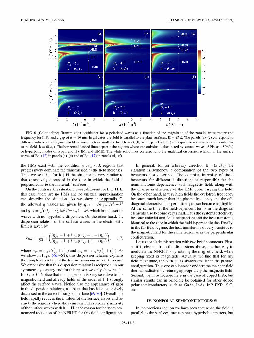
FIG. 6. (Color online) Transmission coefficient for p-polarized waves as a function of the magnitude of the parallel wave vector andfrequency for InSb and a gap of d = 10 nm. In all cases the field is parallel to the plate surfaces, H = Hx x. The panels (a)–(c) correspond todifferent values of the magnetic field for wave vectors parallel to field, k = (kx,0), while panels (d)–(f) correspond to wave vectors perpendicularto the field, k = (0,ky). The horizontal dashed lines separate the regions where transmission is dominated by surface waves (SPPs and SPhPs)or hyperbolic modes of type I and II (HMI and HMII). The white solid lines correspond to the analytical dispersion relation of the surfacewaves of Eq. (12) in panels (a)–(c) and of Eq. (17) in panels (d)–(f).

the HMs exist with the condition εxxεzz < 0, regions thatprogressively dominate the transmission as the field increases.Thus we see that for k ‖ H the situation is very similar tothat extensively discussed in the case in which the field isperpendicular to the materials’ surfaces.

On the contrary, the situation is very different for k ⊥ H. Inthis case, there are no HMs and no uniaxial approximationcan describe the situation. As we show in Appendix C,the allowed q values are given by qo,1 =

√εxxω2/c2 − k2

and qo,2 =√

(ε2yy + ε2

yz)ω2/(c2εyy) − k2, which both describe

waves with no hyperbolic dispersion. On the other hand, thedispersion relation of the surface waves in the electrostaticlimit is given by

kSW = 1

2dln

((ηyy − 1 + iηyz)(ηyy − 1 − iηyz)

(ηyy + 1 + iηyz)(ηyy + 1 − iηyz)

), (17)

where ηyy = εyy/(ε2yy + ε2

yz) and ηyz = −εyz/(ε2yy + ε2

yz). Aswe show in Figs. 6(d)–6(f), this dispersion relation explainsthe complex structure of the transmission maxima in this case.We emphasize that this dispersion relation is reciprocal in oursymmetric geometry and for this reason we only show resultsfor ky > 0. Notice that this dispersion is very sensitive to themagnetic field and already fields of the order of 1 T stronglyaffect the surface waves. Notice also the appearance of gapsin the dispersion relations, a subject that has been extensivelydiscussed in the case of a single interface [69,70]. Overall, thefield rapidly reduces the k values of the surface waves and re-stricts the regions where they can exist. This strong sensitivityof the surface waves with k ⊥ H is the reason for the more pro-nounced reduction of the NFRHT for this field configuration.

In general, for an arbitrary direction k = (kx,ky) thesituation is somehow a combination of the two types ofbehaviors just described. The complex interplay of thesebehaviors for different k directions is responsible for thenonmonotonic dependence with magnetic field, along withthe change in efficiency of the HMs upon varying the field.On the other hand, at very high fields the cyclotron frequencybecomes much larger than the plasma frequency and the off-diagonal elements of the permittivity tensor become negligible.At the same time, the field-dependent terms in the diagonalelements also become very small. Thus the systems effectivelybecome uniaxial and field independent and the heat transfer isidentical to the case in which the field is perpendicular. Finally,in the far-field regime, the heat transfer is not very sensitive tothe magnetic field for the same reason as in the perpendicularconfiguration.

Let us conclude this section with two brief comments. First,as it is obvious from the discussions above, another way tomodulate the NFRHT is by rotating the magnetic field, whilekeeping fixed its magnitude. Actually, we find that for anyfield magnitude, the NFRHT is always smaller in the parallelconfiguration. Thus one can increase or decrease the near-fieldthermal radiation by rotating appropriately the magnetic field.Second, we have focused here in the case of doped InSb, butsimilar results can in principle be obtained for other dopedpolar semiconductors, such as GaAs, InAs, InP, PbTe, SiC,etc.

IV. NONPOLAR SEMICONDUCTORS: Si

In the previous section we have seen that when the field isparallel to the surfaces, one can have hyperbolic emitters, but

125418-8


the HMs always coexist to some degree with surface waves(even at the highest field). We show in this section that in thecase of nonpolar semiconductors, where phonons do not playany role, it is possible to tune the system with a magnetic fieldto a situation where only HMs contribute to the NFRHT. Forthis purpose, we choose Si as the material for the two plates. Asmentioned in the Introduction, it has been predicted [43,44],and experimentally tested [23,27], that in doped Si the NFRHTin the absence of field can be dominated by SPPs even at roomtemperature. Let us see now how this is modified upon applyinga magnetic field.

The dielectric properties of doped Si are similar to thoseof InSb, the only difference being the absence of a phononcontribution. Thus the dielectric functions of Eq. (11) nowread

ε1(H ) = ε∞

(1 + ω2

p(ω + iγ )

ω[ω2

c − (ω + iγ )2])

,

ε3 = ε∞

(1 − ω2

p

ω(ω + iγ )

), (18)

while ε2(H ) remains unchanged. Using the results of Ref. [43]for the dielectric constant of doped Si, we focus on aroom temperature case where the electron concentration isn = 9.3 × 1016 cm−3, ε∞ = 11.7, γ = 8.04 × 1012 rad/s,m∗/m = 0.27, and ωp = 9.66 × 1012 rad/s. We have chosenthis doping level to have a situation in which the plasmafrequency is not too high so that we can affect the NFRHTwith a magnetic field, and not too low so that the NFRHT inthe absence of field is still dominated by SPPs.

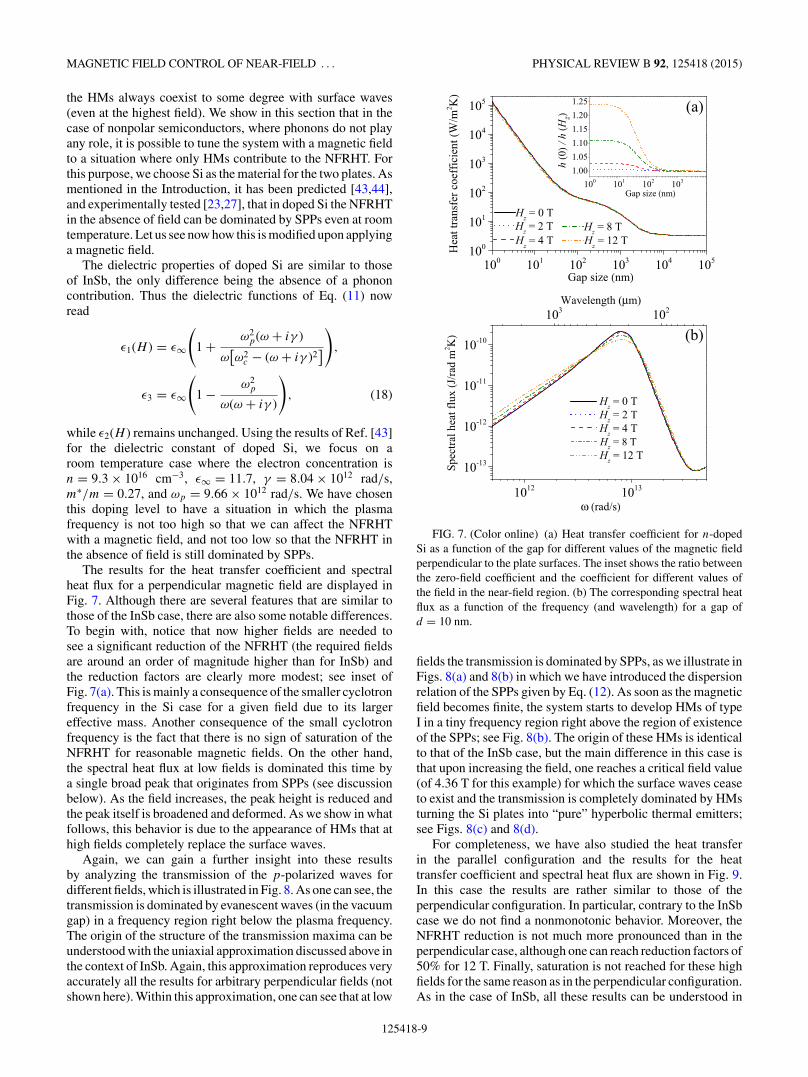
The results for the heat transfer coefficient and spectralheat flux for a perpendicular magnetic field are displayed inFig. 7. Although there are several features that are similar tothose of the InSb case, there are also some notable differences.To begin with, notice that now higher fields are needed tosee a significant reduction of the NFRHT (the required fieldsare around an order of magnitude higher than for InSb) andthe reduction factors are clearly more modest; see inset ofFig. 7(a). This is mainly a consequence of the smaller cyclotronfrequency in the Si case for a given field due to its largereffective mass. Another consequence of the small cyclotronfrequency is the fact that there is no sign of saturation of theNFRHT for reasonable magnetic fields. On the other hand,the spectral heat flux at low fields is dominated this time bya single broad peak that originates from SPPs (see discussionbelow). As the field increases, the peak height is reduced andthe peak itself is broadened and deformed. As we show in whatfollows, this behavior is due to the appearance of HMs that athigh fields completely replace the surface waves.

Again, we can gain a further insight into these resultsby analyzing the transmission of the p-polarized waves fordifferent fields, which is illustrated in Fig. 8. As one can see, thetransmission is dominated by evanescent waves (in the vacuumgap) in a frequency region right below the plasma frequency.The origin of the structure of the transmission maxima can beunderstood with the uniaxial approximation discussed above inthe context of InSb. Again, this approximation reproduces veryaccurately all the results for arbitrary perpendicular fields (notshown here). Within this approximation, one can see that at low

100 101 102 103 104 105100

101

102

103

104

105

(b)

Gap size (nm)

Hea

ttra

nsfe

rcoe

ffic

ient

(W/m

2 K)

(a)

Hz = 0 THz = 2 THz = 4 T

Hz = 8 THz = 12 T

Hz = 0 THz = 2 THz = 4 T

Hz = 12 T

1012 1013

10-13

10-12

10-11

10-10

Spec

tralh

eatf

lux

(J/ra

dm

2 K)

ω (rad/s)

Hz = 8 T

100 101 102 103

1.001.051.101.151.201.25

h(0

)/h

(Hz)

Gap size (nm)

103 102Wavelength (μm)

FIG. 7. (Color online) (a) Heat transfer coefficient for n-dopedSi as a function of the gap for different values of the magnetic fieldperpendicular to the plate surfaces. The inset shows the ratio betweenthe zero-field coefficient and the coefficient for different values ofthe field in the near-field region. (b) The corresponding spectral heatflux as a function of the frequency (and wavelength) for a gap ofd = 10 nm.

fields the transmission is dominated by SPPs, as we illustrate inFigs. 8(a) and 8(b) in which we have introduced the dispersionrelation of the SPPs given by Eq. (12). As soon as the magneticfield becomes finite, the system starts to develop HMs of typeI in a tiny frequency region right above the region of existenceof the SPPs; see Fig. 8(b). The origin of these HMs is identicalto that of the InSb case, but the main difference in this case isthat upon increasing the field, one reaches a critical field value(of 4.36 T for this example) for which the surface waves ceaseto exist and the transmission is completely dominated by HMsturning the Si plates into “pure” hyperbolic thermal emitters;see Figs. 8(c) and 8(d).

For completeness, we have also studied the heat transferin the parallel configuration and the results for the heattransfer coefficient and spectral heat flux are shown in Fig. 9.In this case the results are rather similar to those of theperpendicular configuration. In particular, contrary to the InSbcase we do not find a nonmonotonic behavior. Moreover, theNFRHT reduction is not much more pronounced than in theperpendicular case, although one can reach reduction factors of50% for 12 T. Finally, saturation is not reached for these highfields for the same reason as in the perpendicular configuration.As in the case of InSb, all these results can be understood in

125418-9


FIG. 8. (Color online) Transmission coefficient for p-polarized waves as a function of the magnitude of the parallel wave vector andfrequency for Si and a gap of d = 10 nm. The different panels correspond to different values of the magnetic field that is perpendicular to thesurfaces. The horizontal dashed lines separate the regions where transmission is dominated by surface plasmon polaritons (SPPs) or hyperbolicmodes of type I (HMI). The white solid lines correspond to the analytical SPP dispersion relation of Eq. (12).

terms of the modes that govern the near-field thermal radiation.In this sense, for a direction where k ‖ H, the SPPs thatdominate the NFRHT at low fields are progressively replacedby HMIs upon increasing the field and above 4.36 T they “eatout” all surface waves. On the contrary, for k ⊥ H there are noHMs and the only magnetic field effect is the modification of

100 101 102 103 104 105100

101

102

103

104

105

(b)

Gap size (nm)

Hea

ttra

nsfe

rcoe

ffic

ient

(W/m

2 K)

(a)

Hx = 0 THx = 2 THx = 4 T

Hx = 8 THx = 12 T

Hx = 0 THx = 2 THx = 4 T

Hx = 12 T

1012 1013

10-13

10-12

10-11

10-10

Spec

tralh

eatf

lux

(J/ra

dm

2 K)

ω (rad/s)

Hx = 8 T

100 101 102 103

1.01.11.21.31.41.5

h(0

)/h

(Hx)

Gap size (nm)

103 102Wavelength (μm)

FIG. 9. (Color online) (a) Heat transfer coefficient for n-dopedSi as a function of the gap for different values of the magnetic fieldapplied along the surfaces of the plates. The inset shows the ratiobetween the zero-field coefficient and the coefficient for differentvalues of the field in the near-field region. (b) The correspondingspectral heat flux as a function of the frequency (and wavelength) fora gap of d = 10 nm.

the SPP dispersion relation. Again, the interplay between thesetwo characteristic behaviors among the different k directionsexplains the evolution of the NFRHT with the field.

Let us conclude this section by saying that the behaviorreported here for Si could also be observed for other nonpolarsemiconductors such as Ge.

V. OUTLOOK AND CONCLUSIONS

The results reported in this work raise numerous inter-esting questions. Thus, for instance, in all cases analyzedso far, we have found that the magnetic field reduces theNFRHT as compared to the zero-field result. Is there anyfundamental argument that forbids a magnetic field inducedenhancement? In principle, there is no such an argument.The reduction that we have found in doped semiconductorsis due to the fact that we have explored cases where surfacewaves, which are extremely efficient, dominate the NFRHTin the absence of field. In this sense, one may wonder ifa field-induced enhancement could take place in a situationwhere the NFRHT in the absence of field is dominated bystandard frustrated internal reflection modes, as it happens inmetals [75]. Obviously, metals are out of the question due totheir huge plasma frequency, but one can investigate nonpolarsemiconductors with a low doping level. Indeed, we have doneit for the case of Si and, again, we find that the magnetic fieldreduces the NFRHT and, moreover, exceedingly high fields arerequired to see any significant effect. Of course, we have by nomeans exhausted all possibilities and, for instance, we have notexplored asymmetric situations with different materials. Thusthe question remains of whether the application of a magneticfield can under certain circumstances enhance the near-fieldthermal radiation.

The discovery in this work of the induction of hyperbolicmodes upon the application of a magnetic field may alsohave important consequences for layered structures involvingthin films. Recently, it has been demonstrated that thin filmsmade of polar dielectrics may support NFRHT enhancementscomparable to those of bulk samples when the gap size issmaller than the film thickness [26], which is due to theexcitation of SPhPs. Since the NFRHT in doped semicon-ductors is also dominated by surface electromagnetic waves,all the field-induced effects discussed in this work will also

125418-10


take place in thin films of these materials. However, therecould be quantitative differences. The hyperbolic modes havea propagating character inside the material and, therefore,they may be severely affected in a thin film geometry bythe presence of a substrate. Thus one could expect muchmore dramatic magnetic-field effects in systems coated withsemiconductor thin films.

Obviously, the question remains of whether one canmodulate the NFRHT with a magnetic field in other classesof materials. For instance, since a magneto-optical activityis required, what about ferromagnetic materials? Ideally, onecould imagine to tune the NFRHT by playing around withthe relative orientation of the magnetization, following thespin-valve experiments in the context of spintronics.

Another question of general interest for the field ofmetamaterials is if a doped semiconductor under a magneticfield could exhibit the plethora of exotic optical propertiesreported in hybrid hyperbolic metamaterials [49,50]. We haveshown here that it can behave as a hyperbolic thermal emitter,but can it also exhibit negative refraction or be used to dosubwavelength imaging and focusing in the infrared? Theseare very important questions that we are currently pursuing.

So, in summary, we have presented in this work a verydetailed theoretical analysis of the influence of a magnetic fieldin the NFRHT. By considering the simple case of two parallelplates, we have demonstrated that for doped semiconductorsthe near-field thermal radiation can be strongly modified bythe application of an external magnetic field. In particular, wehave shown that the magnetic field may significantly reduce theNFRHT and the reduction in polar semiconductors can be aslarge as 700% at room temperature. Moreover, we have shownthat when the field is perpendicular to the parallel plates, dopedsemiconductors become ideal hyperbolic thermal emitters withhighly tunable properties. This provides a unique opportunityto explore the physics of thermal radiation in this class ofmetamaterials without the need to resort to complex hybridstructures. Finally, all the predictions of this work are amenableto measurements with the present experimental techniques,and we are convinced that the multiple open questions thatthis work raises will motivate many new theoretical andexperimental studies of this subject.

ACKNOWLEDGMENTS

This work was financially supported by the Colombianagency COLCIENCIAS, the Spanish Ministry of Economyand Competitiveness (Contracts No. FIS2014-53488-P andNo. MAT2014-58860-P), and the Comunidad de Madrid (Con-tract No. S2013/MIT-2740). V.F.-H. acknowledges financialsupport from “la Caixa” Foundation and F.J.G.-V. from theEuropean Research Council (ERC-2011-AdG Proposal No.290981).

APPENDIX A: SCATTERING MATRIX APPROACH FORANISOTROPIC MULTILAYER SYSTEMS

Our analysis of the radiative heat transfer in the presence ofa static magnetic field is based on the combination of Rytov’sfluctuational electrodynamics (FE) and a scattering matrixformalism that describes the propagation of electromagneticwaves in multilayer systems made of optically anisotropic

materials. As we show in Appendix B, the radiative heattransfer can be expressed in terms of the scattering matrixof our system. Thus it is convenient to first discuss in thisappendix the scattering matrix approach employed in this workignoring for the moment the fluctuating currents that generatethe thermal radiation. Later, in Appendix B, we show how thisapproach can be combined with FE. We follow here Ref. [76],which presents a generalization of the formalism introducedby Whittaker and Culshaw in Ref. [77] for isotropic systems.

Let us first describe the Maxwell’s equations to besolved. Assuming a harmonic time dependence exp(−iωt),the Maxwell’s equations for nonmagnetic materials and in theabsence of currents adopt the following form: ∇ · ε0εE = 0,∇ · H = 0, ∇ × H = −iωε0εE, and ∇ × E = iωμ0H, wherethe permittivity is in general a tensor given by Eq. (1). The firstMaxwell’s equation is automatically satisfied if the third one isfulfilled, and the second one can be satisfied by expanding themagnetic field in terms of basis functions with zero divergence.Following Ref. [77], it is convenient to introduce the rescaling:ωε0E → E and

√μ0ε0ω = ω/c → ω. Thus the final two

equations to be solved are

∇ × H = −iεE, (A1)

∇ × E = iω2H. (A2)

We consider here a planar multilayer system grown alongthe z direction in which the tensor ε is constant inside everylayer, i.e., it is independent of the in-plane coordinates r ≡(x,y). Thus, for an in-plane wave vector k ≡ (kx,ky), we canwrite the fields as

H(r,z) = h(z)eik·r and E(r,z) = e(z)eik·r. (A3)

With this notation, Eqs. (A1) and (A2) can be rewritten as

ikyhz(z) − h′y(z) = −i

∑j

εxj ej (z), (A4)

h′x(z) − ikxhz(z) = −i

∑j

εyj ej (z), (A5)

ikxhy(z) − ikyhx(z) = −i∑

j

εzj ej (z), (A6)

and

ikyez(z) − e′y(z) = iω2hx(z), (A7)

e′x(z) − ikxez(z) = iω2hy(z), (A8)

ikxey(z) − ikyex(z) = iω2hz(z), (A9)

where the primes stand for ∂z.Now our task is to solve the Maxwell’s equations for an

unbounded layer. For this purpose, we write the magnetic fieldh(z) as follows:

h(z) = eiqz

{φx x + φy y − 1

q(kxφx + kyφy)z

}, (A10)

where x, y, and z are the Cartesian unit vectors and q isthe z component of the wave vector. Here, φx and φy arethe expansion coefficients to be determined by substituting

125418-11


into Maxwell’s equations. Notice that this expression satisfies∇ · H = 0. Now, it is convenient to rewrite the previousexpression in the vector notation:

h(z) = eiqz

(φx,φy, − 1

q(kxφx + kyφy)

)T

. (A11)

With this notation, Eqs. (A4)–(A6) can be written as

Ch(z) = εe(z), where C =

⎛⎜⎝

0 q −ky

−q 0 kx

ky −kx 0

⎞⎟⎠. (A12)

On the other hand, Eqs. (A7)–(A9) adopt now the form

CT e(z) = ω2h(z). (A13)

From Eq. (A12) we obtain the following expression for theelectric field:

e(z) = ηCh(z), (A14)

where η = ε−1. Substituting this expression in Eq. (A13) weobtain the following equation for the magnetic field:

CT ηCh(z) = ω2h(z), (A15)

which defines an eigenvalue problem for ω2. Indeed, onlytwo of the three identities obtained from this equation, onefor each x, y, and z, are independent. From the first twoidentities, and using Eq. (A11), we obtain the followingequations determining the allowed values for q:(

A2q2 + A1q + A0 + A−1

1

q

)φ = 0, (A16)

where φ = (φx,φy)T and the 2 × 2 matrices An are defined by

A2 =(

ηyy −ηyx

−ηxy ηxx

), A1 = A(a)

1 + A(b)1 =

(−kyηzy kyηzx

kxηzy −kxηzx

)+

(−kyηyz kxηyz

kyηxz −kxηxz

),

A0 = A(a)0 + A(b)

0 − ω21 =(

k2yηzz −kxkyηzz

−kxkyηzz k2xηzz

)+

(k2xηyy − kxkyηyx kxkyηyy − k2

yηyx

kxkyηxx − k2xηxy k2

yηxx − kxkyηxy

)− ω2

(1 0

0 1

),

A−1 =(

k2ykxηzx − k2

xkyηzy k3yηzx − k2

ykxηzy

k3xηzy − k2

xkyηzx k2xkyηzy − k2

ykxηzx

). (A17)

This eigenvalue problem leads to the following quartic secular equation:∑4

n=0 Dnqn = 0, where the coefficients are given by

D4 = ηxxηyy − ηxyηyx,

D3 = kx[ηxyηyz + ηyxηzy − ηyy(ηxz + ηzx)] + ky[ηyxηxz + ηxyηzx − ηxx(ηyz + ηzy)],

D2 = k2x[ηyy(ηxx + ηzz) − ηxyηyx − ηyzηzy] + k2

y[ηxx(ηyy + ηzz) − ηxyηyx − ηxzηzx]

+ kxky[ηxz(ηyz + ηzy) + ηyz(ηzx − ηxz)ηzz(ηxy + ηyx)] − ω2(ηxx + ηyy),

D1 = k3x[ηxyηyz + ηyxηzy − ηyy(ηxz + ηzx)] + k3

y[ηyxηxz + ηxyηzx − ηxx(ηyz + ηzy)]

+ k2xky[ηxyηzx + ηxzηyx − ηxx(ηyz + ηzy)] + k2

ykx[ηyxηzy + ηyzηxy − ηyy(ηxz + ηzx)]

+ω2[k2x(ηxz + ηzx) + k2

y(ηyz + ηzy)],

D0 = k4x(ηyyηzz − ηyzηzy) + k4

y(ηxxηzz − ηxzηzx) + k3xky[ηxzηzy + ηyzηzx − ηzz(ηxy + ηyx)]

+ k3ykx[ηyzηzx + ηxzηzy − ηzz(ηyx + ηxy)] + k2

xk2y[ηzz(ηxx + ηyy) + ηxyηyx − ηxzηzx − ηyzηzy]

+ω2[ω2 − k2x(ηyy + ηzz) − k2

y(ηxx + ηzz) + kxky(ηxy + ηyx)]. (A18)

In general, this secular equation has to be solved numerically,but in many situations of interest the allowed values for q canbe obtained analytically (see Appendix C). The solution ofEq. (A16) provides four complex eigenvalues for q; two lie inthe upper half of the complex plane and the other two in thelower half.

The next step toward the solution of the Maxwell’sequations in a multilayer structure is the determination of thefields in the different layers. This can be done by expressing thefields as a combination of forward and backward propagatingwaves with wave numbers qn (with n = 1,2), and complexamplitudes an and bn, respectively. These amplitudes will

be determined later by using the boundary conditions at theinterfaces and surfaces of the multilayer structure. Since theboundary conditions are simply the continuity of the in-planefield components, we focus here on the analysis of the fieldcomponents ex , ey , hx , and hy . From Eq. (A11), the in-planecomponents of h can be expanded in terms of propagatingwaves as follows:

(hx(z)hy(z)

)=

2∑n=1

{(φxn

φyn

)eiqnzan +

(ϕxn

ϕyn

)e−ipn(d−z)bn

},

(A19)

125418-12


where d is the thickness of the layer. Here, an is the coefficientof the forward going wave at the z = 0 interface, and bn isthe backward going wave at z = d. On the other hand, qn

correspond to the eigenvalues of Eq. (A16) with Im{qn} > 0and pn are the eigenvalues with Im{pn} < 0.

To simplify the notation, we now define two 2 × 2 matrices�+ and �− whose columns are the vectors φn and ϕn,respectively. Moreover, we define the diagonal 2 × 2 matricesf+(z) and f−(d − z), such that [f+(z)]nn = eiqnz and [f−(d −z)]nn = e−ipn(d−z), and the two-dimensional vectors h‖(z) =(hx(z),hy(z))T , a = (a1,a2)T , and b = (b1,b2)T . In terms ofthese quantities, the in-plane magnetic field componentsbecome

h‖(z) = �+ f+(z)a + �−f−(d − z)b. (A20)

Similarly, from Eq. (A14) it is straightforward to showthat the in-plane components of the electric field, e‖(z) =(−ey(z),ex(z))T , are given by

e‖(z) = (A(b)

0 �+q−1 + A(b)1 �+ + A2�+q

)f+(z)a

+ (A(b)

0 �−p−1 + A(b)1 �− + A2�−p

)f−(d − z)b,

(A21)

where the A’s are defined in Eq. (A17) and we have definedthe 2 × 2 diagonal matrices q and p such that qnn = qn andpnn = pn.

We can now combine Eq. (A20) and (A21) into a singleexpression as follows:(

e‖(z)

h‖(z)

)= M

(f+(z)a

f−(d − z)b

)

=(

M11 M12

M21 M22

)(f+(z)a

f−(d − z)b

), (A22)

where the 2 × 2 matrices Mij are defined as

M11 = A(b)0 �+q−1 + A(b)

1 �+ + A2�+q,

M12 = A(b)0 �−p−1 + A(b)

1 �− + A2�−p,

M21 = �+, M22 = �−. (A23)

The final step in our calculation is to use the scatteringmatrix (S matrix) to compute the field amplitudes neededto describe the different relevant physical quantities. Bydefinition, the S matrix relates the vectors of the amplitudesof forward and backward going waves, al and bl , where l nowdenotes the layer, in the different layers of the structure, asfollows:(

al

bl′

)= S(l′,l)

(al′

bl

)=

(S11 S12

S21 S22

)(al′

bl

). (A24)

The field amplitudes in two consecutive layers are relatedvia the continuity of the in-plane components of the fieldsin every interface and surface. If we consider the interfacebetween the layer l and the layer l + 1, this continuity leads to(

e‖(dl)

h‖(dl)

)l

=(

e‖(0)

h‖(0)

)l+1

, (A25)

where dl is the thickness of layer l. From this condition,together with Eq. (A22), it is easy to show that the amplitudesin layers l and l + 1 are related by the interface matrixI (l,l + 1) = M−1

l Ml+1 in the following way:(f +

l al

bl

)= I (l,l + 1)

(al+1

f −l+1bl+1

)

=(

I11 I12

I21 I22

)(al+1

f −l+1bl+1

), (A26)

where f +l = fl,+(dl) and f −

l+1 = fl+1,−(dl+1).Now, with the help of the interface matrices, the S matrix

can be calculated in an iterative way as follows. The matrixS(l′,l + 1) can be calculated from S(l′,l) using the definitionof S(l′,l) in Eq. (A24) and the interface matrix I (l,l + 1).Eliminating al and bl we obtain the relation between al′ , bl′

and al+1, bl+1, from which S(l′,l + 1) can be constructed. Thisreasoning leads to the following iterative relations

S11(l′,l + 1) = [I11 − f +l S12(l′,l)I21]−1f +

l S11(l′,l),

S12(l′,l + 1) = [I11 − f +l S12(l′,l)I21]−1

×(f +l S12(l′,l)I22 − I12)f −

l+1,

S21(l′,l + 1) = S22(l′,l)I21S11(l′,l + 1) + S21(l′,l),

S22(l′,l + 1) = S22(l′,l)I21S12(l′,l + 1) + S22(l′,l)I22f−l+1.

(A27)

Starting from S(l′,l′) = 1, one can apply the previous recursiverelations to a layer at a time to build up S(l′,l). Let us concludethis appendix by saying that from the knowledge of the S

matrix one can easily compute the field amplitudes in everylayer and, in turn, the fields everywhere in the system [77].

APPENDIX B: THERMAL RADIATION IN ANISOTROPICMULTILAYER SYSTEMS

In this Appendix we show how the scattering matrixapproach of Appendix A can be used to describe the thermal ra-diation between planar multilayer systems made of anisotropicmaterials. For this purpose, we first discuss how a genericemission problem can be formulated in the framework of theS-matrix formalism and then, we show how such a formulationcan be used to describe the thermal emission of a multilayersystem.

1. Emission in the scattering matrix approach

For concreteness, let us assume that there is a set of oscillat-ing point sources, with harmonic time dependence, occupyingthe whole plane defined by z = z′. The corresponding electriccurrent density J is given by

J(r,z) = J0δ(z − z′) = j0eik·rδ(z − z′), (B1)

where j0(k) = J0e−ik·r. This current density enters as a source

term in Ampere’s law, Eq. (A1), which now becomes ∇ × H =J − iεE, while Eq. (A2) (Faraday’s law) remains unchanged.

125418-13


Thus Eqs. (A4)–(A6) adopt now the following form:

ikyhz(z) − h′y(z) = j0xδ(z − z′) − i

∑j

εxj ej (z), (B2)

h′x(z) − ikxhz(z) = j0yδ(z − z′) − i

∑j

εyj ej (z), (B3)

ikxhy(z) − ikyhx(z) = j0zδ(z − z′) − i∑

j

εzj ej (z). (B4)

The presence of the source term induces discontinuities inthe fields across the plane z = z′, as we proceed to show. First,let us consider the effect of the in-plane components of thecurrent density by putting jz = 0. To cancel the singular termdue to the source in Eqs. (B2) and (B3), there must be discon-tinuities in hx and hy at z = z′ equal to j0y and −j0x , respec-tively. All the other field components are continuous, exceptfor ez that exhibits a discontinuity equal to (kxj0x + kyj0y)/εzz

in virtue of Eq. (B4). Let us analyze now the role of theperpendicular component of J by putting j0x = j0y = 0. FromEq. (B4), it is clear that in this case ez must contain a singularityto cancel the singular term associated to the current source,that is ez(z) = −i(j0z/εzz)δ(z − z′)+ nonsingular parts. Thisintroduces singular terms in the left-hand side of the MaxwellEqs. (A7) and (A8), which are canceled by discontinuitiesin ex and ey equal to kxj0z/εzz and kyj0z/εzz, respectively.Additionally, it is obvious from Eqs. (B2) and (B3) thathx and hy acquired discontinuities equal to −εyzj0z/εzz andεxzj0z/εzz, respectively. Defining the following vectors:

p‖ = (j0y − εyzj0z/εzz, − j0x + εxzj0z/εzz)T , (B5)

pz = (−kyj0z/εzz,kxj0z/εzz)T , (B6)

the boundary conditions on the in-plane components of thefields are thus

e‖(z′+) − e‖(z′−) = pz, h‖(z′+) − h‖(z′−) = p‖. (B7)

These discontinuity conditions can now be combined withthe S-matrix formalism of the previous appendix to calculatethe emission throughout the system. Let us consider that theemission plane defines the interface between layers l and l + 1in our multilayer structure. Thus the boundary conditions inthis interface become(

e‖(0)

h‖(0)

)l+1

−(

e‖(dl)

h‖(dl)

)l

=(

pz

p‖

). (B8)

Using now the expression of the fields in terms of the layermatrices (M’s), see Eq. (A22), we can write

Ml+1

(al+1

f −l+1bl+1

)− Ml

(f +

l al

bl

)=

(pz

p‖

). (B9)

The external boundary conditions for an emission problemis that there should be only outgoing waves, that is a0 = bN =0, where 0 denotes here the first layer of the structure and N

the last one. Using the definitions of the S matrices S(0,l) andS(l + 1,N ) from Eq. (A24), it follows that

al = S12(0,l)bl , (B10)

bl+1 = S21(l + 1,N )al+1. (B11)

Substituting for al and bl+1 from Eqs. (B10) and (B11) inEq. (B9) and rearranging things, we arrive at the followingcentral result:

(M11,l+1 + M12,l+1f

−l+1S21(l + 1,N ) −[M12,l + M11,l f

+l S12(0,l)]

M21,l+1 + M22,l+1f−l+1S21(l + 1,N ) −[M22,l + M21,l f

+l S12(0,l)]

)(al+1

bl

)=

(pz

p‖

), (B12)

which allows us to compute the field amplitudes on the left andon the right-hand side of the emitting plane. From the solutionof this matrix equation we can compute the field amplitudeeverywhere inside and outside the multilayer structure fromthe knowledge of the scattering matrix.

2. Radiative heat transfer

Let us now show that the previous results can be used todescribe the radiative heat transfer. First of all, we need tospecify the properties of the electric currents that generate thethermal radiation. In the framework of fluctuational electro-dynamics [9], the thermal emission is generated by randomcurrents J inside the material. While the statistical averageof these currents vanishes, i.e., 〈J〉 = 0, their correlations aregiven by the fluctuation-dissipation theorem [78,79]

〈Jk(R,ω)J ∗l (R′,ω′)〉 = 4ε0ωc

π�(ω,T )δ(R − R′)δ(ω − ω′)

×[εkl(R,ω) − ε∗lk(R,ω)]/(2i), (B13)

where R = (r,z) and �(ω,T ) = �ωc/[exp(�ωc/kBT ) − 1], Tbeing the absolute temperature. Let us remind the reader thatwith the rescaling introduced at the beginning of Appendix A,ω has dimensions of wave vector in our notation. Notice that inthe expression of �(ω,T ) a term equal to �ωc/2 that accountsfor vacuum fluctuations has been omitted since it does notaffect the neat radiation heat flux. Notice also that we are usinghere the most general form of this theorem that is suitable fornonreciprocal systems. The fact that the current correlationsare local in space and diagonal in frequency space reducesthe problem of the thermal radiation to the description of theemission by point sources for a given frequency, parallel wavevector, and position inside the structure. Thus we can directlyapply the results derived in the previous subsection.

Let us now consider our system of study, namely twoparallel plates at temperatures T1 and T3 separated by a vacuumgap of width d; see Fig. 10. Our strategy to compute the netradiative heat transfer between the two plates follows closelythat of the seminal work by Polder and Van Hove [7]. First,we compute the radiation power per unit of area transferred

125418-14


0 21 3

(left plate) (right plate) (vacuum gap)

a1 b0

Emitting plane

z d

00 11

(left plate)

aa1bb00

EmEmitittiting plane

g

zz

33

(right plate)

FIG. 10. (Color online) Two parallel plates separated by a vac-uum gap of width d . The vertical dashed line inside the left plateindicates the position of an emitting plane that contains the radiationsources that generate the field amplitudes b0 and a1.

from the left plate to the right one, Q1→3. For this purpose,we first compute the statistical average of the z component ofthe Poynting vector describing the power emitted from a planelocated at z = z′ inside the left plate for a given frequency andparallel wave vector and then we integrate integrate the resultover all possible values of z′, ω, and k, i.e.,

Q1→3(d,T1) =∫ ∞

0dω

∫dk

∫ ∞

0dz′〈Sz(ω,k,z′)〉. (B14)

A similar calculation for the power Q3→1 transferred from theright plate to the left one completes the computation of the nettransferred power per unit of area.

Let us focus now on the analysis of the power emitted bya plane inside the left plate; see Fig. 10. This emitting planedefines a fictitious interface between layers 0 and 1, which areboth inside the left plate. To determine the power emitted tothe right plate we first compute the field amplitudes a1 on theright-hand side of the plane. For this purpose we make use ofEq. (B12), where in this case l = 0 and N = 3. Taking intoaccount that S12(0,0) = 0, it is straightforward to show that

a1 = [M11,1 − M12,1M

−122,1M21,1

]−1pz

+ [M21,1 − M22,1M−112,1M11,1]−1 p‖

= [M−1

1

]11 pz + [

M−11

]12 p‖. (B15)

To compute Q1→3, it is convenient to calculate the Poyntingvector in the vacuum gap. For this purpose, we need the fieldamplitudes in that layer. From Eq. (A24), it is easy to deducethat these amplitudes are given in terms of a1 as follows:

a2 = DS11(1,2)a1, (B16)

where D ≡ [1 − S12(1,2)S21(2,3)]−1 and

b2 = [1 − S21(2,3)S12(1,2)

]−1S21(2,3)S11(1,2)a1

= S21(2,3)a2. (B17)

It is worth stressing that the different elements of the scatteringmatrix that appear in the previous expressions can be factorizedinto scattering matrices S containing only information aboutthe interfaces of the layered system, which are basically theFresnel coefficients of the structure, and phase factors describ-ing the propagation between these interfaces. In particular,

from Eq. (A27) it is easy to show that

S11(1,2) = S11(1,2)f +1 (z′), (B18)

S12(1,2) = S12(1,2)eiq2d , (B19)

S21(2,3) = S21(2,3)eiq2d , (B20)

where q2 = √ω2 − k2 is the z component of the wave vector

in the vacuum gap and

f +1 (z′) =

(eiq1,1z

′0

0 eiq2,1z′

). (B21)

Here, qi,1 (with i = 1,2) are the z components of the twoallowed wave vectors in the medium 1. On the other hand,the S matrices can be computed directly from the interfacematrices as follows [see Eq. (A27)]:

S11(1,2) = I−111 (1,2), (B22)

S12(1,2) = −I−111 (1,2)I12(1,2), (B23)

S21(2,3) = I21(2,3)I−111 (2,3). (B24)

In terms of the amplitudes a2 and b2, the fields in thevacuum gap at z = 0 are given by [see Eq. (A22)](

e‖(0)

h‖(0)

)2

=(

M11,2[a2 − eiq2d b2

]a2 + eiq2d b2

), (B25)

where we have used that M12,2 = −M11,2, valid for anyisotropic system. Thus the z component of the Poynting vectorevaluated at z = 0 in the vacuum gap reads

Sz(ω,k,z′) = 1

4ω

√μ0

ε0{h†

‖(0)e‖(0) + e†‖(0)h‖(0)}2

= 1

4ω

√μ0

ε0{a†

2(M11,2 + M†11,2)a2

−ei(q2−q∗2 )d b†2(M11,2 + M

†11,2)b2

+e−iq∗2 d b†2(M11,2 − M

†11,2)a2

−eiq2d a†2(M11,2 − M

†11,2)b2}. (B26)

Moreover, since

M11,2 = 1

q2

(ω2 − k2

y kxky

kxky ω2 − k2x

)≡ 1

q2A (B27)

and q2 is either real (for k < ω) or purely imaginary (for k > ω),Eq. (B26) reduces to

Sz(ω,k,z′) = 1

2q2ω

√μ0

ε0

×{

a†2Aa2 − b†2Ab2, k < ω,

e−iq∗2 d b†2Aa2 − eiq2d a†

2Ab2, k > ω,

(B28)

where the first term provides the contribution of propagatingwaves and the second one corresponds to the contribution ofevanescent waves.

125418-15


From this point on, the rest of the calculation is pure algebraand we will not describe it here in detail. Let us simply saythat the basic idea is to use Eqs. (B16) and (B17) to express thePoynting vector in Eq. (B28) in terms of the field amplitude a1.Then, using Eq. (B15) and the fluctuation-dissipation theoremof Eq. (B13) one can calculate the statistical average of thePoynting vector. Let us mention that the calculation can begreatly simplified by rotating every 2 × 2 matrix appearingin the problem from the Cartesian basis (x-y) to the basis ofs- and p-polarized waves. This can be done via the unitarymatrix

R ≡ 1

k

(kx ky

ky −kx

), (B29)

which is the matrix that defines the transformation thatdiagonalizes the matrix A, i.e.,

Ad ≡ RAR =(

ω2 0

0 q22

). (B30)

Finally, after integrating over all possible values of ω, k, and z′,see Eq. (B14), one arrives at the following result for the powerper unit of area transferred from the left plate to the right one:

Q1→3(d,T1) =∫ ∞

0

dω

2π�(ω,T1)

∫dk

(2π )2τ (ω,k,d), (B31)

where τ (ω,k,d) is the total transmission coefficient of theelectromagnetic modes and it is given by

τ (ω,k,d) ={

Tr{[1 − S12(1,2)S†12(1,2)]D†[1 − S

†21(2,3)S21(2,3)]D}, k < ω (propagating waves),

Tr{[S12(1,2) − S†12(1,2)]D†[S†

21(2,3) − S21(2,3)]D}e−2|q2|d , k > ω (evanescent waves).(B32)

Here, the 2 × 2 matrices indicated by a bar are defined asfollows:

D ≡ A1/2d RDRA

−1/2d , (B33)

D† ≡ A−1/2d RD†RA

1/2d . (B34)

Following a similar reasoning, one can compute the powerper unit of area transfer from the right plate to the left one andthe final result reads

Q3→1(d,T3) =∫ ∞

0

dω

2π�(ω,T3)

∫dk

(2π )2τ (ω,k,d), (B35)

where τ (ω,k,d) is also given by Eq. (B32). Thus the netpower per unit of area exchanged by the plates is given byEqs. (2) and (3) in Sec. II. To conclude, let us stress that in themanuscript ω is meant to be an angular frequency.

APPENDIX C: DISPERSION RELATIONS

In this appendix we provide the solution of the eigenvalueproblem of Eqs. (A16) and (A17) that give the dispersionrelations of the electromagnetic modes that can exist insidethe materials considered in this work. In particular, we focushere on three cases of special interest for our discussions inthe main body of the manuscript.

Case 1: ε = diag[εxx,εxx,εzz]. This situation is of relevancefor the case in which the magnetic field is perpendicular to theplate surfaces; see Sec. III A. In this case, the allowed q valuesare given by

q2o = εxxω

2 − k2, q2e = εxxω

2 − k2εxx/εzz. (C1)

Case 2: ε = diag[εxx,εzz,εzz]. This situation is relevant forthe case in which the magnetic field is parallel to the platesurfaces, see Sec. III B, and the allowed q values are given by

q2o = εzzω

2 − k2, q2e = εxxω

2 − k2εxx/εzz. (C2)

Case 3: the diagonal elements of ε are εxx and εyy =εzz, while the only nonvanishing off-diagonal elements are

εyz = −εzy . This situation is relevant for the case in which themagnetic field is parallel to the plate surfaces; see Sec. III B.In this case, the allowed q values adopt the following form:

q2o,1 = εxxω

2 − k2, q2o,2 = (

ε2yy + ε2

yz

)ω2/εyy − k2. (C3)

APPENDIX D: SURFACE ELECTROMAGNETIC MODES

We briefly describe here how we determine the dispersionrelation of the surface electromagnetic modes in our systemand we also provide the results for some configurations ofspecial interest.

Let us consider a structure containing N planar layers. FromEq. (A26), it is easy to show that the field amplitudes in layersl and l + 1 are related as follows:

(al

bl

)=

(f +

l 0

0 1

)−1

I (l,l + 1)

(1 0

0 f −l+1

)(al+1

bl+1

)

≡ I ′(l,l + 1)

(al+1

bl+1

). (D1)

Now, using this relation recursively we can relate the fieldamplitudes in the first and last layers as follows:

(a1

b1

)=

[N−1∏l=1

I ′(l,l + 1)

](aN

bN

)≡ I S

(aN

bN

). (D2)

The condition for an eigenmode of the system is thata1 = bN = 0, which from the previous equation implies thatI S

11aN = 0. The condition for having a nontrivial solution ofthis equation is that det I S

11 = 0, which is the condition thatsurface electromagnetic modes must satisfy. In our plate-plategeometry, the 4 × 4 matrix I S is simply given by

I S = I (1,2)

(e−iq2d 1 0

0 eiq2d 1

)I (2,3), (D3)

125418-16


where let us recall that q2 = √ω2 − k2. Thus the condition for

an eigenmode of the system reads

det[I11(1,2)I11(2,3)e−iq2d + I12(1,2)I21(2,3)eiq2d ] = 0.

(D4)

In what follows, we provide the explicit equations satisfied bythe dispersion relation of the surface waves in the three casesconsidered in Appendix C.

Case 1. In this case, Eq. (D4) leads to

e−iq2d = ±(

qe − εxxq2

qe + εxxq2

), (D5)

where qe is given in Eq. (C1). This equation reduces to Eq. (12)in the electrostatic limit k � ω/c.

Case 2. Here, assuming that the surface wave propagatesalong the x direction, its dispersion relation satisfies the

following relation:

e−iq2d = ±(

qe − εxxq2

qe + εxxq2

), (D6)

where qe is given in Eq. (C2). In the electrostatic limit, thisequation reduces to Eq. (12).

Case 3. In this case, and assuming that the surface wavespropagate along the y direction, its dispersion relation is givenby the solution of the following equation:

e−2iq2d = (ηyyqo,2 − q2 + ηyzk)(ηyyqo,2 − q2 − ηyzk)

(ηyyqo,2 + q2 + ηyzk)(ηyyqo,2 + q2 − ηyzk),

(D7)

where ηyy = εyy/(ε2yy + ε2

yz), ηyz = −εyz/(ε2yy + ε2

yz), and qo,2

is given in Eq. (C3). In the electrostatic limit this equationreduces to Eq. (17).

[1] R. Siegel and J. R. Howell, Thermal Radiation Heat Transfer,4th ed. (Taylor and Francis, New York, 2002).

[2] Z. M. Zhang, Nano/microscale Heat Transfer (McGraw-Hill,New York, 2007).

[3] K. Joulain, J. P. Mulet, F. Marquier, R. Carminati, and J. J.Greffet, Surf. Sci. Rep. 57, 59 (2005).

[4] A. I. Volokitin and B. N. J. Persson, Rev. Mod. Phys. 79, 1291(2007).

[5] S. Basu, Z. M. Zhang, and C. J. Fu, Int. J. Energy Res. 33, 1203(2009).

[6] B. Song, A. Fiorino, E. Meyhofer, and P. Reddy, AIP Adv. 5,053503 (2015).

[7] D. Polder and M. Van Hove, Phys. Rev. B 4, 3303 (1971).[8] S. M. Rytov, Theory of Electric Fluctuations and Thermal

Radiation (Air Force Cambridge Research Center, Bedford,MA, 1953).

[9] S. M. Rytov, Y. A. Kravtsov, and V. I. Tatarskii, Principlesof Statistical Radiophysics (Springer-Verlag, Berlin, 1989),Vol. 3.

[10] C. M. Hargreaves, Phys. Lett. A 30, 491 (1969).[11] G. A. Domoto, R. F. Boehm, and C. L. Tien, J. Heat Transfer

92, 412 (1970).[12] A. Kittel, W. Muller-Hirsch, J. Parisi, S.-A. Biehs, D. Reddig,

and M. Holthaus, Phys. Rev. Lett. 95, 224301 (2005).[13] A. Narayanaswamy, S. Shen, and G. Chen, Phys. Rev. B 78,

115303 (2008).[14] L. Hu, A. Narayanaswamy, X. Y. Chen, and G. Chen, Appl.

Phys. Lett. 92, 133106 (2008).[15] E. Rousseau, A. Siria, G. Jourdan, S. Volz, F. Comin, J. Chevrier,

and J.-J. Greffet, Nat. Photon. 3, 514 (2009).[16] S. Shen, A. Narayanaswamy, and G. Chen, Nano Lett. 9, 2909

(2009).[17] R. S. Ottens, V. Quetschke, S. Wise, A. A. Alemi, R. Lundock,

G. Mueller, D. H. Reitze, D. B. Tanner, and B. F. Whiting, Phys.Rev. Lett. 107, 014301 (2011).

[18] S. Shen, A. Mavrokefalos, P. Sambegoro, and G. Chen, Appl.Phys. Lett. 100, 233114 (2012).

[19] T. Kralik, P. Hanzelka, M. Zobac, V. Musilova, T. Fort, andM. Horak, Phys. Rev. Lett. 109, 224302 (2012).

[20] P. J. van Zwol, L. Ranno, and J. Chevrier, Phys. Rev. Lett. 108,234301 (2012).

[21] P. J. van Zwol, S. Thiele, C. Berger, W. A. de Heer, and J.Chevrier, Phys. Rev. Lett. 109, 264301 (2012).

[22] B. Guha, C. Otey, C. B. Poitras, S. H. Fan, and M. Lipson, NanoLett. 12, 4546 (2012).

[23] J. Shi, P. Li, B. Liu, and S. Shen, Appl. Phys. Lett. 102, 183114(2013).

[24] L. Worbes, D. Hellmann, and A. Kittel, Phys. Rev. Lett. 110,134302 (2013).

[25] R. St-Gelais, B. Guha, L. X. Zhu, S. H. Fan, and M. Lipson,Nano Lett. 14, 6971 (2014).

[26] B. Song, Y. Ganjeh, S. Sadat, D. Thompson, A. Fiorino, V.Fernandez-Hurtado, J. Feist, F. J. Garcia-Vidal, J. C. Cuevas, P.Reddy, and E. Meyhofer, Nat. Nanotechnol. 10, 253 (2015).

[27] M. Lim, S. S. Lee, and B. J. Lee, Phys. Rev. B 91, 195136(2015).

[28] W. A. Challener, C. B. Peng, A. V. Itagi, D. Karns, W. Peng,Y. Y. Peng, X. M. Yang, X. B. Zhu, N. J. Gokemeijer, Y. T. Hsia,G. Ju, R. E. Rottmayer, M. A. Seigler, and E. C. Gage, Nat.Photon. 3, 220 (2009).

[29] B. C. Stipe, T. C. Strand, C. C. Poon, H. Balamane, T. D. Boone,J. A. Katine, J. L. Li, V. Rawat, H. Nemoto, A. Hirotsune, O.Hellwig, R. Ruiz, E. Dobisz, D. S. Kercher, N. Robertson, T. R.Albrecht, and B. D. Terris, Nat. Photon. 4, 484 (2010).

[30] J. B. Pendry, J. Phys.: Condens. Matter 11, 6621 (1999).[31] Y. D. Wilde, F. Formanek, R. Carminati, B. Gralak, P. A.

Lemoine, K. Joulain, J. P. Mulet, Y. Chen, and J. J. Greffet,Nature (London) 444, 740 (2006).

[32] A. Kittel, U. F. Wischnath, J. Welker, O. Huth, F. Ruting, andS. A. Biehs, Appl. Phys. Lett. 93, 193109 (2008).

[33] A. C. Jones, B. T. O’Callahan, H. U. Yang, and M. B. Raschke,Prog. Surf. Sci. 88, 349 (2013).

[34] R. Carminati and J. J. Greffet, Phys. Rev. Lett. 82, 1660(1999).

[35] J. J. Greffet, R. Carminati, K. Joulain, J. P. Mulet, S. P. Mainguy,and Y. Chen, Nature (London) 416, 61 (2002).

[36] C. R. Otey, W. T. Lau, and S. Fan, Phys. Rev. Lett. 104, 154301(2010).

125418-17

http://dx.doi.org/10.1016/j.surfrep.2004.12.002




http://dx.doi.org/10.1103/RevModPhys.79.1291




http://dx.doi.org/10.1002/er.1607




http://dx.doi.org/10.1063/1.4919048

http://dx.doi.org/10.1063/1.4919048

http://dx.doi.org/10.1063/1.4919048

http://dx.doi.org/10.1063/1.4919048





http://dx.doi.org/10.1016/0375-9601(69)90264-3

http://dx.doi.org/10.1016/0375-9601(69)90264-3

http://dx.doi.org/10.1016/0375-9601(69)90264-3

http://dx.doi.org/10.1016/0375-9601(69)90264-3

http://dx.doi.org/10.1115/1.3449677

http://dx.doi.org/10.1115/1.3449677

http://dx.doi.org/10.1115/1.3449677

http://dx.doi.org/10.1115/1.3449677

http://dx.doi.org/10.1103/PhysRevLett.95.224301








http://dx.doi.org/10.1063/1.2905286

http://dx.doi.org/10.1063/1.2905286

http://dx.doi.org/10.1063/1.2905286

http://dx.doi.org/10.1063/1.2905286

http://dx.doi.org/10.1038/nphoton.2009.144




http://dx.doi.org/10.1021/nl901208v








http://dx.doi.org/10.1063/1.4723713

http://dx.doi.org/10.1063/1.4723713

http://dx.doi.org/10.1063/1.4723713

http://dx.doi.org/10.1063/1.4723713













http://dx.doi.org/10.1021/nl301708e




http://dx.doi.org/10.1063/1.4804631

http://dx.doi.org/10.1063/1.4804631

http://dx.doi.org/10.1063/1.4804631

http://dx.doi.org/10.1063/1.4804631





http://dx.doi.org/10.1021/nl503236k




http://dx.doi.org/10.1038/nnano.2015.6
















http://dx.doi.org/10.1088/0953-8984/11/35/301

http://dx.doi.org/10.1088/0953-8984/11/35/301

http://dx.doi.org/10.1088/0953-8984/11/35/301

http://dx.doi.org/10.1088/0953-8984/11/35/301

http://dx.doi.org/10.1038/nature05265




http://dx.doi.org/10.1063/1.3025140

http://dx.doi.org/10.1063/1.3025140

http://dx.doi.org/10.1063/1.3025140

http://dx.doi.org/10.1063/1.3025140

http://dx.doi.org/10.1016/j.progsurf.2013.07.001








http://dx.doi.org/10.1038/416061a

http://dx.doi.org/10.1038/416061a

http://dx.doi.org/10.1038/416061a

http://dx.doi.org/10.1038/416061a






[37] A. W. Rodriguez, O. Ilic, P. Bermel, I. Celanovic, J. D.Joannopoulos, M. Soljacic, and S. G. Johnson, Phys. Rev. Lett.107, 114302 (2011).

[38] P. Ben-Abdallah and S. A. Biehs, Phys. Rev. Lett. 112, 044301(2014).

[39] R. Messina and P. Ben-Abdallah, Sci. Rep. 3, 1383 (2013).[40] A. Lenert, D. M. Bierman, Y. Nam, W. R. Chan, I. Celanovic,

M. Soljacic, and E. N. Wang, Nat. Nanotechnol. 9, 126 (2014).[41] J. W. Schwede, I. Bargatin, D. C. Riley, B. E. Hardin, S. J.

Rosenthal, Y. Sun, F. Schmitt, P. Pianetta, R. T. Howe, Z. X.Shen, and N. A. Melosh, Nat. Mater. 9, 762 (2010).

[42] J. P. Mulet, K. Joulain, R. Carminati, and J. J. Greffet, MicroscaleTherm. Eng. 6, 209 (2002).

[43] C. J. Fu and Z. M. Zhang, Int. J. Heat Mass Transfer 49, 1703(2006).

[44] E. Rousseau, M. Laroche, and J. J. Greffet, Appl. Phys. Lett. 95,231913 (2009).

[45] I. S. Nefedov and C. R. Simovski, Phys. Rev. B 84, 195459(2011).

[46] S. A. Biehs, M. Tschikin, and P. Ben-Abdallah, Phys. Rev. Lett.109, 104301 (2012).

[47] Y. Guo, C. L. Cortes, S. Molesky, and Z. Jacob, Appl. Phys.Lett. 101, 131106 (2012).

[48] D. R. Smith and D. Schurig, Phys. Rev. Lett. 90, 077405 (2003).[49] A. Poddubny, I. Iorsh, P. Belov, and Y. Kivshar, Nat. Photon. 7,

948 (2013).[50] P. Shekhar, J. Atkinson, and Z. Jacob, Nano Convergence 1, 14

(2014).[51] S. A. Biehs, M. Tschikin, R. Messina, and P. Ben-Abdallah,

Appl. Phys. Lett. 102, 131106 (2013).[52] M. Tschikin, S. A. Biehs, R. Messina, and P. Ben-Abdallah,

J. Opt. 15, 105101 (2013).[53] Y. Guo and Z. B. Jacob, Opt. Express 21, 15014 (2013).[54] C. Simovski, S. Maslovski, I. Nefedov, and S. Tretyakov, Opt.

Express 21, 14988 (2013).[55] X. L. Liu, R. Z. Zhang, and Z. M. Zhang, Appl. Phys. Lett. 103,

213102 (2013).[56] X. L. Liu, R. Z. Zhang, and Z. M. Zhang, Int. J. Heat Mass

Transfer 73, 389 (2014).[57] Y. Guo and Z. Jacob, J. Appl. Phys. 115, 234306 (2014).[58] O. D. Miller, S. G. Johnson, and A. W. Rodriguez, Phys. Rev.

Lett. 112, 157402 (2014).

[59] S. Lang, M. Tschikin, S. A. Biehs, A. Yu. Petrov, and M. Eich,Appl. Phys. Lett. 104, 121903 (2014).

[60] I. S. Nefedov and L. A. Melnikov, Appl. Phys. Lett. 105, 161902(2014).

[61] M. Tschikin, S. A. Biehs, P. Ben-Abdallah, S. Lang, A. Yu.Petrov, and M. Eich, J. Quant. Spectrosc. Radiat. Transf. 158,17 (2015).

[62] P. J. van Zwol, K. Joulain, P. Ben-Abdallah, and J. Chevrier,Phys. Rev. B 84, 161413(R) (2011).

[63] P. J. van Zwol, K. Joulain, P. Ben Abdallah, J. J. Greffet, andJ. Chevrier, Phys. Rev. B 83, 201404(R) (2011).

[64] L. J. Cui, Y. Huang, and J. Wang, J. Appl. Phys. 112, 084309(2012).

[65] Y. Huang, S. V. Boriskina, and G. Chen, Appl. Phys. Lett. 105,244102 (2014).

[66] K. Chen, P. Santhanam, S. Sandhu, L. Zhu, and S. Fan, Phys.Rev. B 91, 134301 (2015).

[67] A. Zvezdin and V. Kotov, Modern Magnetooptics and Magne-tooptical Materials (IOP, Bristol, 1997).

[68] S. A. Biehs, P. Ben-Abdallah, F. S. S. Rosa, K. Joulain, and J.-J.Greffet, Opt. Express 19, A1088 (2011).

[69] M. S. Kushwaha, Surf. Sci. Rep. 41, 1 (2001).[70] R. F. Wallis, in Electromagnetic Surface Modes, edited by A. D.

Boardman (Wiley, New York, 1982), p. 575.[71] E. D. Palik, B. Kaplan, B. W. Gammon, H. Kaplan, J. J. Quinn,

and B. F. Wallis, Phys. Lett. A 45, 143 (1973).[72] A. Hartstein, E. Burstein, E. D. Palik, R. W. Gammon, and

B. W. Henvis, Phys. Rev. B 12, 3186 (1975).[73] E. D. Palik, R. Kaplan, R. W. Gammon, H. Kaplan, R. F. Wallis,

and J. J. Quinn, Phys. Rev. B 13, 2497 (1976).[74] L. Remer, E. Mohler, W. Grill, and B. Luthi, Phys. Rev. B 30,

3277 (1984).[75] P. O. Chapuis, S. Volz, C. Henkel, K. Joulain, and J. J. Greffet,

Phys. Rev. B 77, 035431 (2008).[76] B. Caballero, A. Garcıa-Martın, and J. C. Cuevas, Phys. Rev. B

85, 245103 (2012).[77] D. M. Whittaker and I. S. Culshaw, Phys. Rev. B 60, 2610

(1999).[78] L. Landau, E. Lifshitz, and L. Pitaevskii, Course of Theoretical

Physics (Pergamon, New York, 1980), Vol. 9, Part 2.[79] Yu. A. Il’inskii and L. V. Keldysh, Electromagnetic Response of

Material Media (Plenum Press, New York, 1994).

125418-18









http://dx.doi.org/10.1038/srep01383








http://dx.doi.org/10.1038/nmat2814




http://dx.doi.org/10.1080/10893950290053321

http://dx.doi.org/10.1080/10893950290053321

http://dx.doi.org/10.1080/10893950290053321

http://dx.doi.org/10.1080/10893950290053321

http://dx.doi.org/10.1016/j.ijheatmasstransfer.2005.09.037




http://dx.doi.org/10.1063/1.3271681

http://dx.doi.org/10.1063/1.3271681

http://dx.doi.org/10.1063/1.3271681

http://dx.doi.org/10.1063/1.3271681









http://dx.doi.org/10.1063/1.4754616

http://dx.doi.org/10.1063/1.4754616

http://dx.doi.org/10.1063/1.4754616

http://dx.doi.org/10.1063/1.4754616









http://dx.doi.org/10.1186/s40580-014-0014-6

http://dx.doi.org/10.1186/s40580-014-0014-6

http://dx.doi.org/10.1186/s40580-014-0014-6

http://dx.doi.org/10.1186/s40580-014-0014-6

http://dx.doi.org/10.1063/1.4800233

http://dx.doi.org/10.1063/1.4800233

http://dx.doi.org/10.1063/1.4800233

http://dx.doi.org/10.1063/1.4800233

http://dx.doi.org/10.1088/2040-8978/15/10/105101

http://dx.doi.org/10.1088/2040-8978/15/10/105101

http://dx.doi.org/10.1088/2040-8978/15/10/105101

http://dx.doi.org/10.1088/2040-8978/15/10/105101

http://dx.doi.org/10.1364/OE.21.015014

http://dx.doi.org/10.1364/OE.21.015014

http://dx.doi.org/10.1364/OE.21.015014

http://dx.doi.org/10.1364/OE.21.015014

http://dx.doi.org/10.1364/OE.21.014988

http://dx.doi.org/10.1364/OE.21.014988

http://dx.doi.org/10.1364/OE.21.014988

http://dx.doi.org/10.1364/OE.21.014988

http://dx.doi.org/10.1063/1.4832057

http://dx.doi.org/10.1063/1.4832057

http://dx.doi.org/10.1063/1.4832057

http://dx.doi.org/10.1063/1.4832057





http://dx.doi.org/10.1063/1.4883243

http://dx.doi.org/10.1063/1.4883243

http://dx.doi.org/10.1063/1.4883243

http://dx.doi.org/10.1063/1.4883243





http://dx.doi.org/10.1063/1.4869490

http://dx.doi.org/10.1063/1.4869490

http://dx.doi.org/10.1063/1.4869490

http://dx.doi.org/10.1063/1.4869490

http://dx.doi.org/10.1063/1.4899126

http://dx.doi.org/10.1063/1.4899126

http://dx.doi.org/10.1063/1.4899126

http://dx.doi.org/10.1063/1.4899126

http://dx.doi.org/10.1016/j.jqsrt.2014.11.013












http://dx.doi.org/10.1063/1.4759055

http://dx.doi.org/10.1063/1.4759055

http://dx.doi.org/10.1063/1.4759055

http://dx.doi.org/10.1063/1.4759055

http://dx.doi.org/10.1063/1.4904456

http://dx.doi.org/10.1063/1.4904456

http://dx.doi.org/10.1063/1.4904456

http://dx.doi.org/10.1063/1.4904456





http://dx.doi.org/10.1364/OE.19.0A1088




http://dx.doi.org/10.1016/S0167-5729(00)00007-8

http://dx.doi.org/10.1016/S0167-5729(00)00007-8

http://dx.doi.org/10.1016/S0167-5729(00)00007-8

http://dx.doi.org/10.1016/S0167-5729(00)00007-8

http://dx.doi.org/10.1016/0375-9601(73)90462-3

http://dx.doi.org/10.1016/0375-9601(73)90462-3

http://dx.doi.org/10.1016/0375-9601(73)90462-3

http://dx.doi.org/10.1016/0375-9601(73)90462-3

























Documents

Magnetic field control of near-field radiative heat transfer ... · Magnetic field control of near-field radiative heat transfer and the realization of highly tunable hyperbolic