Embed Size (px)
Citation preview

Magnetic Design for High Temperature, High Frequency SiC Power Electronics
Torbjørn Sørsdahl
Master of Energy and Environmental Engineering
Supervisor: Tore Marvin Undeland, ELKRAFT
Department of Electric Power Engineering
Submission date: July 2013
Norwegian University of Science and Technology


2013
i
1 Summary Power electronic components which can operate at high temperatures would benefit a large number
of different applications such as in petroleum exploration, aviation and electrical vehicles. Silicon
carbide semiconductors have in the recent years been introduced commercially in the market. They
are opening up new possibilities to create high temperature devices, due to its superior properties
over silicon. Design of high temperature magnetic components is still a tedious process compared to
normal temperature levels due to little information and software to simplify this process.
The purpose of this thesis is to develop analytical software for high frequency magnetic design in the
temperature range from 130°C, and up to 200°C. Care has been taken into developing temperature
dependent loss models and thermal design. The software is primarily for inductors, but most of the
theory and discussion are also valid for transformers. Prototypes have been built and tested against
the software predictions and good correlation has been observed.
A brief introduction to magnetic materials that can be used at elevated temperatures have been
included focusing on powder cores and ferrites, since other high frequency materials could not
operate at 200°C. It was found that for most materials, it is the laminations and binder agents that
introduce the temperature limit. Materials are designed for specific temperatures which make it
likely that when there is a larger commercial interest for higher temperatures, new materials will be
developed. Core characterization of ferrites and powder cores was performed with a Brochause steel
tester up to 10 kHz, and the losses up to 100 kHz were measured using an oscilloscope and amplifier
approach. The characterization was performed at 20°C 108°C and 180°C.
The measurements show that the analytical loss data provided by the manufacturers underestimates
the losses in Sendust and MPP materials, while there is a good correlation in High Flux, R-ferrite and
N27. New Steinmetz parameters were calculated for MPP and Sendust for 20 kHz. Temperature
primarily influences only Sendust up to 180 °C by a factor of 10-20 %, the little temperature
dependence is in powder cores due to very high curie temperature.
Winding configurations have been investigated, and Litz wire for 200°C do not seem to exist
commercially at this date, however wire for 130°C was successfully used in several 180°C
experiments, but permanent degradation was observed in wires which had been exposed for several
hours. It was found that the insulation in enamel coated round conductors have problems at
elevated temperatures under the rated temperature in the areas where the wire was bent, this was
not observed in Litz wire.
It has been shown that parallel connection of smaller powder cores can in some cases be used to
obtain smaller designs with better thermal dissipation than with a single core. Leakage capacitance
has been measured in several designs and by inserting an air gap between layers the capacitance was
reduced in the same order as a Bank winding.
Output filter for dv/dt, Sinus, and a step down converter have been calculated and built. The step
down filter has been tested in a buck converter, and compared to analytical data.

2013
ii
2 Preface This thesis was started as a summer job at SmartMotor in Trondheim 2012, and continued during my
final year in Energy and Environment. The thesis has been very interesting and I have learned much
on how to design magnetic components at higher temperatures, and how often laboratory
equipment do not work as planned.
During my work on this specialization project there are many people I would like to thank. First I
would like to thank my supervisor Professor Tore M. Undeland for giving me the possibility to work
on this topic, and he’s support. Second the invaluable help of Dr. Richard Lund and his practical
experience in filter and inductor design. Third Professor Arne Nysveen, Edris Agheb and Amir Hayati
Soloot for helping me out with lab equipment, and spending time to show me how to use it. Finally
everyone in the mechanical workshop and the service lab for always being able to help me.
Torbjørn Sørsdahl Trondheim Norway July 2013

2013
iii
Table of Contents
1 SUMMARY ................................................................................................................................................ I
2 PREFACE................................................................................................................................................... II
3 LIST OF FIGURES ..................................................................................................................................... VII
4 LIST OF TABLES ........................................................................................................................................ XI
NOMENCLATURE ........................................................................................................................................... XIII
ABBREVIATION ............................................................................................................................................... XV
1 INTRODUCTION........................................................................................................................................ 1
BACKGROUND ............................................................................................................................................ 1 1.1
PROBLEM DESCRIPTION ................................................................................................................................ 2 1.2
REPORT OUTLINE ........................................................................................................................................ 3 1.3
2 SILICON CARBIDE ..................................................................................................................................... 5
SILICON CARBIDE IN POWER ELECTRONICS ........................................................................................................ 5 2.1
COMPARISON OF SIC TO CONVENTIONAL SWITCHES ........................................................................................... 7 2.2
REFERENCES .............................................................................................................................................. 8 2.3
3 COMPONENTS IN SINUS FILTERS AND DV/DT FILTERS.............................................................................. 9
INTRODUCTION .......................................................................................................................................... 9 3.1
FILTER THEORY ......................................................................................................................................... 10 3.2
CRITICAL CABLE LENGTH ............................................................................................................................. 11 3.3
DV/DT FILTER .......................................................................................................................................... 12 3.4
SINUS OUTPUT FILTER ................................................................................................................................ 13 3.5
SIMULATION MODEL.................................................................................................................................. 14 3.6
REFERENCES ............................................................................................................................................ 16 3.7
4 MAGNETIC MATERIALS .......................................................................................................................... 17
POWDER CORES........................................................................................................................................ 18 4.1
SOFT FERRITES ......................................................................................................................................... 22 4.2
SHAPE .................................................................................................................................................... 23 4.3
PERMEABILITY .......................................................................................................................................... 23 4.4
CORE LOSS .............................................................................................................................................. 26 4.5
REFERENCES ............................................................................................................................................ 28 4.6
5 CORE LOSS ............................................................................................................................................. 29
FLUX WAVEFORMS .................................................................................................................................... 29 5.1
LOSS MODELS .......................................................................................................................................... 30 5.2
PARAMETERS INFLUENCING CORE LOSS .......................................................................................................... 33 5.3
REFERENCES ............................................................................................................................................ 34 5.4
6 WINDING CONFIGURATION ................................................................................................................... 35
INTRODUCTION ........................................................................................................................................ 35 6.1
LITZ WIRE ................................................................................................................................................ 38 6.2
ROUND WIRE ........................................................................................................................................... 39 6.3

2013
iv
FOIL WINDING .......................................................................................................................................... 40 6.4
PARASITIC CAPACITANCES ........................................................................................................................... 41 6.5
REFERENCES ............................................................................................................................................ 44 6.6
7 THERMAL ASPECTS & MODELS ............................................................................................................... 45
INTRODUCTION ........................................................................................................................................ 45 7.1
THERMAL MODELING ................................................................................................................................. 46 7.2
COMSOL MODEL .................................................................................................................................... 46 7.3
HEAT TRANSFER BY CONDUCTION ................................................................................................................. 47 7.4
HEAT TRANSFER BY CONVECTION ................................................................................................................. 48 7.5
NATURAL CONVECTION AND FORCED CONVECTION .......................................................................................... 48 7.6
HEAT TRANSFER BY RADIATION .................................................................................................................... 53 7.7
MOUNTING ............................................................................................................................................. 54 7.8
EMPIRICAL THERMAL MODEL ....................................................................................................................... 55 7.9
MODEL COMPARISON ................................................................................................................................ 56 7.10
WINDING THERMAL RESISTANCE .................................................................................................................. 57 7.11
CORE THERMAL RESISTANCE ........................................................................................................................ 59 7.12
THERMAL MODEL FOR TOROID MAGNETIC COMPONENTS .................................................................................. 60 7.13
EXTERNAL THERMAL RESISTANCE.................................................................................................................. 62 7.14
REFERENCES ............................................................................................................................................ 63 7.15
8 INDUCTOR SOFTWARE ........................................................................................................................... 64
SHORT INTRODUCTION ............................................................................................................................... 64 8.1
LIMITATIONS && GOAL.............................................................................................................................. 64 8.2
INPUT PARAMETERS .................................................................................................................................. 64 8.3
OUTPUT PARAMETERS ............................................................................................................................... 69 8.4
EXPERIMENTAL RESULTS ............................................................................................................................. 69 8.5
REFERENCES ............................................................................................................................................ 70 8.6
9 FILTER DIMENSIONS ............................................................................................................................... 71
FILTER FOR A BUCK CONVERTER ................................................................................................................... 71 9.1
SINUS AND DV/DT FILTER ........................................................................................................................... 73 9.2
9.2.1 RLC Dv/dt Filter ................................................................................................................................ 73
9.2.2 Sinus Filter ....................................................................................................................................... 75
FILTER COMPARISON ................................................................................................................................. 76 9.3
REFERENCES ............................................................................................................................................ 77 9.4
10 LABORATORY SETUP .............................................................................................................................. 78
SAMPLES ................................................................................................................................................. 78 10.1
CORE LOSS CHARACTERIZATION ................................................................................................................... 78 10.2
10.2.1 Measurement setup BROCHAUS MPG ........................................................................................ 78
10.2.2 Core characterisation at 180.5°C ................................................................................................ 81
100 KHZ MEASUREMENTS .......................................................................................................................... 82 10.3
10.3.1 Core Loss measurements ............................................................................................................ 82
10.3.2 Fundamental waveform with a high frequency ripple ................................................................ 84
10.3.3 Non-sinusoidal losses .................................................................................................................. 84
MEASUREMENTS WITH A BUCK CONVERTER................................................................................................... 84 10.4
LEAKAGE CAPACITANCE .............................................................................................................................. 85 10.5
REFERENCES ............................................................................................................................................ 87 10.6

2013
v
11 MEASUREMENTS AND DISCUSSION ....................................................................................................... 88
CORE LOSS .............................................................................................................................................. 88 11.1
11.1.1 Core loss in KoolMµ 5 kHz – 9 kHz .............................................................................................. 88
11.1.2 Core loss in KoolMµ 5 kHz – 100 kHz .......................................................................................... 90
11.1.3 Core loss in High Flux 160 5 kHz – 9.9 kHz .................................................................................. 92
11.1.4 Core loss in High Flux 160 5 kHz – 100 kHz ................................................................................. 93
11.1.5 Core loss in High Flux 125 5 kHz- 9.9 kHz .................................................................................... 94
11.1.6 Core loss in MPP 5 kHz- 9 kHz ..................................................................................................... 95
11.1.7 Core loss in MPP 5 kHz- 100 kHz ................................................................................................. 95
11.1.8 Core loss in N27 Ferrite ............................................................................................................... 97
11.1.9 Core loss in R Ferrite .................................................................................................................... 98
BUCK CONVERTER ..................................................................................................................................... 99 11.2
11.2.1 Inductor measurements and comparison ................................................................................... 99
11.2.2 Paralleling of inductors ............................................................................................................. 100
LEAKAGE CAPACITANCE ............................................................................................................................ 101 11.3
11.3.1 Reducing the leakage capacitance ............................................................................................ 101
11.3.2 Parallel connection between two inductors .............................................................................. 102
11.3.3 Minimum leakage capacitance ................................................................................................. 103
11.3.4 Enamel windings ....................................................................................................................... 104
11.3.5 Leakage capacitance in a hybrid winding of enamel and Litz wire ........................................... 105
11.3.6 Temperature and Leakage capacitance .................................................................................... 105
REFERENCES .......................................................................................................................................... 106 11.4
12 CONCLUSIONS ...................................................................................................................................... 107
13 FURTHER WORK ................................................................................................................................... 109
A APPENDIXES ......................................................................................................................................... 110
B APPENDIX SOFTWARE FOR DESIGN OF POWDER CORES INDUCTORS .................................................. 111
I. TURNS .................................................................................................................................................. 111
II. FILL FACTOR ........................................................................................................................................... 111
III. MEAN LENGTH PER TURN ......................................................................................................................... 111
IV. HDC ..................................................................................................................................................... 113
V. FLUX DENSITY ........................................................................................................................................ 113
VI. PERMEABILITY CORRECTION ...................................................................................................................... 113
VII. THE POWER HANDLING CAPABILITY OF THE CORE ........................................................................................... 113
VIII. RESISTANCE ........................................................................................................................................... 114
IX. POWER LOSS ......................................................................................................................................... 114
X. SURFACE AREA ....................................................................................................................................... 115
XI. THERMAL .............................................................................................................................................. 115
XII. LAYERS ................................................................................................................................................. 115
XIII. LEAKAGE INDUCTANCE ............................................................................................................................. 115
XIV. STACKING CORES .................................................................................................................................... 116
XV. ITERATIVE PROCESS ................................................................................................................................. 116
XVI. REFERENCES .......................................................................................................................................... 117
C APPENDIX SOFTWARE TO DESIGN FERRITE INDUCTORS ....................................................................... 118
I. ENERGY STORAGE CAPABILITY .................................................................................................................... 118
II. PERMEABILITY ........................................................................................................................................ 118

2013
vi
III. REFERENCES .......................................................................................................................................... 119
D APPENDIX MEASUREMENTS & CALCULATIONS .................................................................................... 120
I. MEASUREMENTS UP TO 100 KHZ 20°C ..................................................................................................... 120
II. MEASUREMENTS UP TO 100 KHZ 180°C.................................................................................................... 125
III. NON-SINUSOIDAL LOSSES ......................................................................................................................... 127
V. FILTER FOR BUCK CONVERTER ................................................................................................................... 128
VI. DV/DT OUTPUT INDUCTOR FOR DIFFERENTIAL NOISE ...................................................................................... 129
VII. SINUS OUTPUT FILTER .............................................................................................................................. 130
VIII. PARALLEL CONNECTION OF INDUCTORS IN A BUCK CONVERTER ......................................................................... 132
IX. N27 .................................................................................................................................................... 133
E APPENDIX PYTHON .............................................................................................................................. 134
F MECHANICAL MEASUREMENTS MLT .................................................................................................... 135
G THERMAL RESISTANCES ....................................................................................................................... 136
I. NATURAL CONVECTION............................................................................................................................ 136
II. FORCED CONVECTION .............................................................................................................................. 137
III. RADIATION ............................................................................................................................................ 137
H PICTURES FROM THE LABORATORY ..................................................................................................... 140
I PYTHON SOURCE CODE ........................................................................................................................ 142

2013
vii
3 List of Figures Figure 1-1 Down-hole system .................................................................................................................. 1
Figure 3-1 Differential and Common mode noise [2]............................................................................ 10
Figure 3-2 Low pass filter [1] ................................................................................................................. 10
Figure 3-3 RLC Filter .............................................................................................................................. 11
Figure 3-4 RLC filter at the inverters output ......................................................................................... 12
Figure 3-5 Different sinus filter configurations [7] ................................................................................ 13
Figure 3-6 The PSCAD model of a Buck converter ................................................................................ 14
Figure 3-7 The PSCAD model of the converter with a sinus filter ......................................................... 15
Figure 4-1 Typical B-H Loops for some magnetic materials [3] ............................................................. 17
Figure 4-2 Some powder core shapes ................................................................................................... 18
Figure 4-3 High magnification of a powder material ............................................................................ 18
Figure 4-4 Core loss limited at 100 mWcm-3 for 15.6 cm3 cores at 5 kHz ............................................. 20
Figure 4-5 Core losses for 15.6 cm3 cores up to saturation at 5 kHz ..................................................... 20
Figure 4-6 Core loss limited at 100 mWcm-3 for 15.6 cm3 cores at 100 kHz ......................................... 20
Figure 4-7 Core losses for 15.6 cm3 cores up to saturation at 100 kHz ................................................. 20
Figure 4-8 Core loss with sinus 50 mT peak at 100 kHz compared to rated saturation flux density .... 21
Figure 4-9 Current measurement in an inductor experiencing a .......................................................... 21
Figure 4-10 Comparison of the inductance in koolMµ with increasing Idc .......................................... 24
Figure 4-11 Comparison of the inductance in HighFlux with increasing Idc ......................................... 24
Figure 4-12 Permeability versus dc bias in KoolMµ .............................................................................. 25
Figure 4-13 Permeability versus dc bias for XFlux ................................................................................. 25
Figure 4-14 Permeability versus dc bias for High Flux........................................................................... 25
Figure 4-15 Permeability versus dc bias for MPP .................................................................................. 25
Figure 4-16 Measured loss in N27 at 5 kHz ........................................................................................... 26
Figure 4-17 Measured loss in R ferrite at 5 kHz .................................................................................... 26
Figure 4-18 Measured loss in KoolMµ at 20 kHz ................................................................................... 27
Figure 4-19 Measured loss in KoolMµ at 50 kHz ................................................................................... 27
Figure 4-20 Measured loss in HighFlux at 20 kHz .................................................................................. 27
Figure 4-21 Measured loss in HighFlux at 100 kHz ................................................................................ 27
Figure 4-22 Measured loss in MPP at 20 kHz ........................................................................................ 27
Figure 4-23 Measured loss in MPP at 50 kHz ........................................................................................ 27
Figure 5-1 Flux waveforms [5] ............................................................................................................... 30
Figure 6-1 100 k Hz skin depth at different temperatures .................................................................... 35
Figure 6-2 Proximity effect in multilayer windings ............................................................................... 36
Figure 6-3 Rac/Rdc for Od = 1.25 mm at 25 °C ....................................................................................... 37
Figure 6-4 Rac/Rdc for Od = 1.25 mm at 200 °C ..................................................................................... 37
Figure 6-5 Square fitting ........................................................................................................................ 39
Figure 6-6 Hexagonal fitting .................................................................................................................. 39
Figure 6-7 Damage to enamel insulation operated at 170 °C ............................................................... 40
Figure 6-8 Damage to enamel insulation operated at 180.5 °C ............................................................ 40
Figure 6-9 Inductor equivalent circuit ................................................................................................... 42

2013
viii
Figure 6-10 Impedance versus frequency for a normally wound core ................................................. 43
Figure 6-11 Impedance versus frequency for a bank winding .............................................................. 43
Figure 6-12 Impedance versus frequency for a winding with air gap between the layers ................... 43
Figure 7-1 Toroid mesh ......................................................................................................................... 47
Figure 7-2 Simulation results. ................................................................................................................ 47
Figure 7-3 Boundary layer fluid velocity profile perpendicular to a wall .............................................. 48
Figure 7-4 Boundary layer Temperature profile perpendicular to a wall ............................................. 48
Figure 7-5 The total distance of the boundary layer Lt= a+b+2(d2+e2)0.5 .............................................. 49
Figure 7-6 COMSOL model of a core including only radiation .............................................................. 54
Figure 7-7 Horizontal and vertical mounted cores ................................................................................ 55
Figure 7-8 Heat conduction in a single layer ......................................................................................... 58
Figure 7-9 Heat Conduction in two layers ............................................................................................. 58
Figure 7-10 Heat conduction in three layers ......................................................................................... 58
Figure 7-11 Heat conduction in ten layers ............................................................................................ 58
Figure 7-12 Thermal conductivity for different fill factors [11] ............................................................ 59
Figure 7-13 Heat conduction for non-ideal windings ............................................................................ 59
Figure 7-14 Heat conduction in the core with dins= 0.5 mm ................................................................. 60
Figure 7-15 Heat conduction in the core with dins= 2 mm .................................................................... 60
Figure 7-16 Equivalent thermal circuit .................................................................................................. 61
Figure 8-1 GUI of the Inductor designer ................................................................................................ 65
Figure 9-1 Buck converter [1] ................................................................................................................ 71
Figure 9-2 Buck converter in continues mode [1] ................................................................................. 71
Figure 9-3 Circuit topology of the RLC filter model ............................................................................... 74
Figure 9-4 The voltage waveform before and after the filter ............................................................... 74
Figure 9-5 The voltage and current waveform before the load ........................................................... 74
Figure 9-6 Zoomed in view of the voltage before and after the filter .................................................. 74
Figure 9-7 Zoomed in view of the voltage and current at the load ...................................................... 74
Figure 9-8 Circuit topology of the Sinus filter model ............................................................................ 75
Figure 9-9 The voltage at the load and current ..................................................................................... 75
Figure 9-10 Filtered and unfiltered line to line voltage ......................................................................... 75
Figure 10-1 Control principle for electric sheet measuring instrument [2] .......................................... 79
Figure 10-2 The heating chamber rated for 0°C to 200°C ..................................................................... 80
Figure 10-3 The plugin system for ring cores in BROCHAUS MPG 100D ............................................... 80
Figure 10-4 Measured loss in High Flux at 5 kHz ................................................................................... 83
Figure 10-5 Measured loss in KoolMµ at 5 kHz ..................................................................................... 83
Figure 10-6 Impedance plot for 16 Turns Litz wire 240 strands............................................................ 86
Figure 10-7 Impedance plot for KoolMµ 41 Turns Litz wire 120 strands .............................................. 86
Figure 10-8 Impedance plot for 136 Turns enamel ............................................................................... 86
Figure 10-9 Impedance plot for 165 Turns Litz 120 strands .................................................................. 86
Figure 11-1 Measured loss in KoolMµ at 3 kHz ..................................................................................... 88
Figure 11-2 Measured loss in KoolMµ at 5 kHz ..................................................................................... 89
Figure 11-3 Measured loss in KoolMµ at 7 kHz ..................................................................................... 89
Figure 11-4 Measured loss in KoolMµ at 10 kHz ................................................................................... 89
Figure 11-5 Measured loss in KoolMµ at 5 kHz ..................................................................................... 90

2013
ix
Figure 11-6 Measured loss in KoolMµ at 20 kHz ................................................................................... 90
Figure 11-7 Measured loss in KoolMµ at 50 kHz ................................................................................... 90
Figure 11-8 Measured loss in KoolMµ at 100 kHz ................................................................................. 90
Figure 11-9 Comparison of new Steinmetz parameters for 5 - 20 kHz at 20 kHz ................................ 91
Figure 11-10 Comparison of new Steinmetz parameters for 20 - 50 kHz at 20 kHz ............................. 91
Figure 11-11 Measured loss in HighFlux 160 at 3 kHz ........................................................................... 92
Figure 11-12 Measured loss in HighFlux 160 at 5 kHz ........................................................................... 92
Figure 11-13 Measured loss in HighFlux 160 at 7 kHz ........................................................................... 92
Figure 11-14 Measured loss in HighFlux 160 at 9.9 kHz ........................................................................ 92
Figure 11-15 Measured loss in High Flux at 5 kHz ................................................................................. 93
Figure 11-16 Measured loss in High Flux at 20 kHz ............................................................................... 93
Figure 11-17 Measured loss in High Flux at 50 kHz ............................................................................... 93
Figure 11-18 Measured loss in High Flux at 100 kHz ............................................................................. 93
Figure 11-19 Measured loss in HighFlux 125 at 3 kHz ........................................................................... 94
Figure 11-20 Measured loss in HighFlux 125 at 5 kHz ........................................................................... 94
Figure 11-21 Measured loss in HighFlux 125 at 7 kHz ........................................................................... 94
Figure 11-22 Measured loss in HighFlux 125 at 9.9 kHz ........................................................................ 94
Figure 11-23 Measured loss in MPP 125 at 3 kHz ................................................................................. 95
Figure 11-24 Measured loss in MPP 125 at 5 kHz ................................................................................. 95
Figure 11-25 Measured loss in MPP 125 160 at 7 kHz .......................................................................... 95
Figure 11-26 Measured loss in MPP 125 at 9.9 kHz .............................................................................. 95
Figure 11-27 Measured loss in MPP at 5 kHz ........................................................................................ 96
Figure 11-28 Measured loss in MPP at 20 kHz ...................................................................................... 96
Figure 11-29 Measured loss in MPP at 50 kHz ...................................................................................... 96
Figure 11-30 Measured loss in MPP at 100 kHz .................................................................................... 96
Figure 11-31 Comparison of new Steinmetz parameters for 5 - 20 kHz at 20 kHz .............................. 97
Figure 11-32 Comparison of new Steinmetz parameters for 20 - 50 kHz at 20 kHz ............................. 97
Figure 11-33 Measured loss in N27 at 3 kHz ......................................................................................... 97
Figure 11-34 Measured loss in N27 at 5 kHz ......................................................................................... 97
Figure 11-35 Measured loss in R ferrite at 3 kHz .................................................................................. 98
Figure 11-36 Measured loss in R ferrite at 5 kHz .................................................................................. 98
Figure 11-37 Measured loss in R ferrite at 7 kHz ................................................................................. 98
Figure 11-38 Measured loss in R ferrite at 9 kHz .................................................................................. 98
Figure 11-39 Measured permeability with increasing dc current in 0077715A7 (KoolMµ) ............... 100
Figure 11-40 Measured permeability with increasing dc current C058583A2 (High Flux 160) .......... 100
Figure 11-41 Analytical permeability with increasing dc current in 0077715A7 (KoolMµ) ................ 101
Figure 11-42 Analytical permeability with increasing dc current in C058583A2 (High Flux 160) ....... 101
Figure 11-43 Impedance versus frequency for a normally wound core ............................................. 101
Figure 11-44 Impedance versus frequency for a bank winding .......................................................... 101
Figure 11-45 Impedance versus frequency for a winding with air gap between the layers ............... 102
Figure 11-46 A single 100 turn KoolMµ core ....................................................................................... 102
Figure 11-47 Parallel connection of two 100 turn KoolMµ core ......................................................... 102
Figure 11-48 A 1 turn Litz wire on a KoolMµ core NB add 20 db to the amplitude ............................ 103
Figure 11-49 A 5 turn KoolMµ core NB add 20 db to the amplitude .................................................. 103

2013
x
Figure 11-50 A 8 turn KoolMµ core NB add 20 db to the amplitude .................................................. 103
Figure 11-51 A 11 turn KoolMµ core NB add 20 db to the amplitude ................................................ 104
Figure 11-52 A 100 turn koolMµ core with 100 turns of Litz wire 120 x 0.1mm ................................ 104
Figure 11-53 A 136 turns high flux 160 core with 136 turns of enamel wire 1 x 1.15 mm ................. 104
Figure 11-54 A 100 turn KoolMµ core with 100 turns of Litz wire 120 x 0.1mm ................................ 105
Figure 11-55 A 100 turn KoolMµ core with 100 turns of Litz wire 120 x 0.1mm and 10 turns of enamel
1 x 1.15 mm 20 db need to be added to the vertical axis ................................................................... 105
Figure 11-56 A 100 turn KoolMµ core with 100 turns of Litz wire 120 x 0.1mm at 20°C ................... 106
Figure 11-57 A 100 turn High Flux core with 136 turns of Litz wire 1 x 1.15 at 20°C .......................... 106
Figure 11-58 A 100 turn KoolMµ core with 100 turns of Litz wire 120 x 0.1mm at 118°C ................. 106
Figure 11-59 A 100 turn High Flux core with 136 turns of Litz wire 1 x 1.15 at 118°C ........................ 106
Figure 13-1 Toroid winding configuration ........................................................................................... 112
Figure 13-2 (a) Square fitting (b) hexagonal fitting [4]. ....................................................................... 112
Figure 13-3 Simple flow chart of the Iterative process ....................................................................... 117
Figure 13-4 The loss measurement setup with a Brochause steel tester ........................................... 140
Figure 13-5 The heating chamber ....................................................................................................... 140
Figure 13-6 Buck converter ................................................................................................................. 141
Figure 13-7 The 100 kHz amplifier setup ............................................................................................. 142

2013
xi
4 List of Tables
Table 1-1 Drive Specification ................................................................................................................... 2
Table 2-1 SiC Commercial products with largest breakdown voltage in the market 2012 [6] ............... 5
Table 2-2 SiC material properties compared to Si [8] ............................................................................. 5
Table 2-3 Temperature problems in semiconductors [10] ..................................................................... 6
Table 3-1 Magnetic components in power electronic applications ........................................................ 9
Table 3-2 Desired properties for CM and DM inductors ....................................................................... 10
Table 3-3 Filter parameters for RLC filters [2] ....................................................................................... 12
Table 3-4 Cable parameters .................................................................................................................. 14
Table 4-1 Magnetic Properties of some powder Cores [1][9] ............................................................... 19
Table 4-2 Magnetic Properties of some powder HT Ferrites ................................................................ 22
Table 4-3 Examples of absolute maximum NI that should be applied to magnetics® powder cores ... 24
Table 6-1 Advantages and disadvantages with Litz wires [2]. ............................................................... 38
Table 6-2 Advantages and disadvantages with round wires ................................................................. 39
Table 6-3 Advantages and disadvantages with foil windings ................................................................ 40
Table 6-4 Measured values for a normal winding ................................................................................. 43
Table 6-5 Measured values for a Bank winding .................................................................................... 43
Table 6-6 Measured values an inductor with air gap between layers .................................................. 43
Table 7-1 Thermal classes for inductive modules ................................................................................. 45
Table 7-2 COMSOL Model inputs .......................................................................................................... 46
Table 7-3 Thermal conductivity for some materials [7] ........................................................................ 47
Table 7-4 Thermal conductivity examples............................................................................................. 52
Table 7-5 Thermal properties of Air and Oil [8] T in Celcius ................................................................. 52
Table 7-6 Emissivity of some surfaces [7] ............................................................................................. 53
Table 7-7 Radiation at different temperatures ..................................................................................... 53
Table 7-8 COMSOL model data for C058583A2 .................................................................................... 56
Table 7-9 Comparison of temperature increase in C058583A2 for natural convection ....................... 56
Table 7-10 C058583A2 including windings ........................................................................................... 57
Table 7-11 Temperature comparison in C058548A2 with 106 turns of 120 x 0.1 Litz wires with natural
convection cooling ................................................................................................................................ 57
Table 7-12 Temperature comparison in C058548A2 with 106 turns of 120 x 0.1 Litz wires with natural
convection cooling at 100 °C ambient temperature ............................................................................. 57
Table 7-13 COMSOL model data for the windings ................................................................................ 58
Table 7-14 Thermal conductivity for different configurations with 50 % fill factor .............................. 59
Table 7-15 COMSOL model data for core thermal resistance ............................................................... 59
Table 8-1 Output Parameters ................................................................................................................ 69
Table 9-1 Buck filter specifications ........................................................................................................ 72
Table 9-2 Drive specification ................................................................................................................. 73
Table 9-3 Dv/dt filter values .................................................................................................................. 73
Table 9-4 Sinus filter values ................................................................................................................... 75
Table 9-5 Input parameters ................................................................................................................... 76

2013
xii
Table 9-6 Software recommendations .................................................................................................. 76
Table 10-1 Core materials ..................................................................................................................... 78
Table 10-2 Lab equipment ..................................................................................................................... 79
Table 10-3 Core loss samples ................................................................................................................ 80
Table 10-4 Winding resistance before and after the high temperature tests ...................................... 81
Table 10-5 Lab equipment for 100 kHz ................................................................................................. 82
Table 10-6 Equations to calculate the flux density in the core ............................................................. 82
Table 10-7 Lab equipment Buck converter ........................................................................................... 84
Table 10-8 Inductance and resistivity measurements in some inductors ............................................. 85
Table 10-9 Lab equipment for Leakage capacitance ............................................................................. 85
Table 10-10 Leakage capacitance and SRF in some different inductors ............................................... 86
Table 11-1 KoolMµ new Steinmetz parameters .................................................................................... 91
Table 11-2 MPP new Steinmetz parameters ......................................................................................... 96
Table 11-3 Buck filter properties ........................................................................................................... 99
Table 11-4 Comparison of analytical design and measured values for inductors................................. 99
Table 11-5 Comparison of analytical design and measured values for inductors............................... 100
Table 11-6 Measured values for a normal winding ............................................................................. 101
Table 11-7 Measured values for a Bank winding ................................................................................ 101
Table 11-8 Measured values an inductor with air gap between layers .............................................. 102
Table 11-9 Parameters of a single 100 turn KoolMµ core .................................................................. 102
Table 11-10 Parameters of a parallel connection of two 100 turn KoolMµ core ............................... 102
Table 11-11 Parameters for a 1 turn KoolMµ core ............................................................................. 103
Table 11-12 Parameters for a 5 turn KoolMµ core ............................................................................. 103
Table 11-13 Parameters for a 5 turn KoolMµ core ............................................................................. 103
Table 11-14 Parameters for a 5 turn KoolMµ core ............................................................................. 104
Table 11-15 Litz wire and enamel comparison.................................................................................... 104
Table 11-16 100 Litz wire versus hybrid winding of 100 turn Litz with 10 turns enamel ................... 105
Table 11-17 Leakage capacitance comparison at elevated temperatures .......................................... 106
Table 13-1 The permeability stability in a ferrite air gap 0.26mm le 138mm and µ 2300.................. 118
Table 13-2 measurements from 5 – 100 kHz at 20°C .......................................................................... 120
Table 13-3 measurements from 5 – 100 kHz at 180°C ........................................................................ 125
Table 13-4 Inductor analytical data and measured values ................................................................. 129
Table 13-5 Inductor analytical data and measured values ................................................................. 129
Table 13-6 some values for LC in different filters ............................................................................... 130
Table 13-7 KoolMµ 70 turns inductance at dc bias from 0-16 A ......................................................... 132
Table 13-8 KoolMµ two 100 turns inductors parallel connected ........................................................ 132
Table 13-9 HighFlux 40 turns inductance at dc bias from 0-16 A........................................................ 132
Table 13-10 HighFlux two 50 turns inductors parallel connected ...................................................... 132
Table 13-11 N27 Geometric Data ........................................................................................................ 133

2013
xiii
Nomenclature Symbol Description Unit W Energy J s-1 Al Nominal inductance nH N-2 Flux density in the air gap Wb m-2
Flux density in the magnetic material Wb m-2 Relative permeability 1 Permeability of free space defined to be 4π Henries H·m−1 µ Permeability H·m−1 Cross section area of the air gap m2
Le Mean magnetic path m N Number of turns - B Magnetic flux density Wb m-2 Core thermal resistance K W-1 Winding thermal resistance K W-1 External thermal resistance K W-1
Power loss core W Power loss winding W Ambient temperature K Surface temperature K Flow temperature K T Temperature K ΔT Temperature gradient K m-1 Heat transfer coefficient W m-2K-1 Height of the magnetic component m n Constant - C Constant - Velocity of the flow outside the boundary layer ms-1 The area the flow see of the magnetic component m2 Total distance of the boundary layer m Effective enveloped surface m2
Radius of the wire m Core outer diameter including wire m Core inner diameter including wire m Core height including wire m
𝑦 Core outer diameter mm
Core inner diameter mm
H Height of the magnetic component mm Density m-3 kg Dynamic viscosity N s m-2 Pr Prandtl number - Kinematic viscosity m2s-1 The constant pressure specific heat capacity J kg-1K-1
Thermal conductivity Wm-1K-1 Gr Grashof number - The characteristic length m Gravity constant ms-2 The thermal volume expansion coefficient K-1 The thermal diffusivity m2s-1

2013
xiv
Reynolds number - Nu Nusselt number - ε Permittivity F·cm-2 Rise time s Resonance frequency m-1 fsw Switching frequency m-1 Equivalent frequency m-1
Relative frequency m-1 β Parameter in the Steinmetz equation for flux density change - Parameter in the Steinmetz equation for frequency change - K Parameter in the Steinmetz equation a constant - λ Thermal conductivity W·m-1·°C-1 Band-gap eV
Critical field V·cm-1 µn Electron mobility cm2V-1·s-1 ni Intrinsic concentration cm-3 Ionized acceptor density cm-3 Ionized donor density cm-3 Majority carrier lifetime s
Minority carrier lifetime s q Electron charge C K Boltzmann’s constant J·K-1 Permittivity of vacuum F·cm-2 Relative permittivity - Area between the windings m2 Distance between the different windings m Heat flux Wm-2 w Fluid velocity ms-1 L Inductance H Output voltage V Time period the switch is off s
Current ripple A Switching period s Capacitance F Critical cable length m Cable inductance H Cable capacitance C

2013
xv
Abbreviation Parameter Description SiC Silicon Carbide Si Silicon EMC Electromagnetic Compatibility PCB Printed circuit board ESR Equivalent series resistor HT High Temperature (defined here as above 150°C) DM Differential mode noise CM Common mode noise SRF Self-resonance frequency

Introduction 2013
1
1 Introduction
Background 1.1
High temperature power devices such as converters and inverters are becoming more and more
important in applications like petroleum exploration, aviation and electrical vehicles. The trend is to
push the devices into even harsher environments. Electrification of down-hole drilling equipment is a
promising area which requires electrical components that are able to withstand the high ambient
temperatures, and pressure several kilometers subsurface. SmartMotor and Badger Explorer are
developing a motor drive for a down-hole drilling tool with the concept as following:
“The Badger Explorer is a revolutionary method to obtain subsurface data for oil gas exploration,
mapping of hydrocarbon resources and long-term surveillance. The Badger Explorer drills and buries
underground, carrying a unique package of logging and monitoring sensors, at a substantially lower
risk, cost and complexity of utilizing an expensive drilling rig.”
Figure 1-1 shows a possible overview of this concept.
The conventional switching technology is based on silicon (Si) devices which is limited in a range of
properties compared to silicon carbide (SiC). SiC offers better thermal conductivity, band gap,
breakdown field and are capable of being operated at high junction temperatures. However the
main deceleration factors in developing new applications are the packing technology, control
electronics and passive components.
Figure 1-1 Down-hole system

Introduction 2013
2
Problem description 1.2
This master thesis will focus on the design of fast magnetic components for high temperature power
devices, the task description is as follows:
The aim is to develop an analytical design tool in Python for fast magnetic/electrical/ thermal calculation of typical magnetic components used in high temperature power electronics. Due to wide operating temperature ranges exact temperature dependent loss models are required. Also, compactness requires more accurate thermal models and effective cooling.
Comparison of SiC and conventional switches in terms of influence on the magnetic components should be carried out. The analytical results should be compared with experimental results.
The materials required to design magnetic components for temperatures up to 200°C will be
surveyed. A comparison between SiC and Si will be performed. Loss models for magnetic materials
will be compared to lab measurements performed at 20°C and 200°C in the frequency range from 3
kHz to 100 kHz. A thermal model for inductors will be developed and compared to measurements,
and the information gathered will be used to create an analytical design tool for high temperature
and frequency up to 100 kHz.
The tool will be used to design sinus and dv/dt filters for the electrical specification in Table 1-1, and
the cores recommended by the tool will be tested and evaluated.
Table 1-1 Drive Specification
Drive Specification
Vdc 600 V S 3000 VA fsw Up to 100 kHz Tamb 150 °C
1 kV/µs
Where Vdc is the Dc-link voltage S is the apparent power delivered fsw is the switching frequency Tamb is the downhole ambient temperature dv/dt is the maximum voltage change over given time

Introduction 2013
3
Report outline 1.3
Chapter 2
This chapter presents silicon carbide and compares the theoretical properties to silicon. Theory on
semiconductor devices is used to perform a comparison on the influence of using SiC over Si on the
magnetic components.
Chapter 3
Different magnetic components will be introduced and filter theory for dv / dt and sinus will be
explained. Simulation of the different filters will performed to some extent with a focus on reducing
the component physical size.
Chapter 4
Magnetic materials for inductor design are presented, and the most common materials are
explained. Thereafter suitable ferrites and powder materials for 200°C power electronics is
investigated. Theory and some recommendations for reducing the core size in powder materials is
then explained, and finally core losses measured in the materials is presented, and compared to the
analytical data up to 100 kHz.
Chapter 5 Core losses and flux waveforms are explained in more detail, and analytical models on how to
calculate core loss is presented. The most recent models are listed and different parameters that
affect the core losses are mentioned.
Chapter 6 The possible winding options for inductors are explained with a focus on Litz, round and foil
windings. Thereafter experience and problems with using round enamel windings and Litz wire at
180°C is briefly covered. The last section covers theory and ways to reduce parasitic capacitance.
Chapter 7 Basic thermal modelling in inductors is explained and the thermal conductivity of Litz wire and
multilayer windings is investigated with COMSOL Multiphysics. A tthermal model of round cores is
developed for forced and natural convection, and simulated in COMSOL Multiphysics. Lab
measurements of a high frequency Litz wire windings is performed and compared to the analytical
results at 22°C and 100°C.
Chapter 8 Chapter 8 presents the analytical design tool. Input and output parameters are explained and ways
to input data for different applications is explained. Some analytical designs are compared to
experimental measurements.
Chapter 9 The design tool and information from chapter 3 is used to design sinus, buck and dv/dt filters.

Introduction 2013
4
Chapter 10 This chapter covers the different lab setups which was performed, and explains relevant theory and error sources. There were four different lab setups:
Core characterization 3 kHz -10 kHz
Core characterization 5 kHz -100 kHz
Inductor measurements in a buck converter
Leakage capacitance in windings
Chapter 11 Chapter 11 presents the measurement results in more details than the other chapters and the results are evaluated and discussed. Chapter 12 Chapter 12 presents the conclusion.
Chapter 13
Chapter 13 covers further work.

Silicon Carbide 2013
5
2 Silicon Carbide Silicon (Si) is the conventional material used in the production of power devices, while Silicon carbide
(SiC) is a material which has proven to have superior properties and has recently become
commercially available, but still lags behind Si in some aspects by as much as 20 years. However
some applications can have tremendous benefits from SiC due to higher temperature limit and very
low losses.
Silicon Carbide in power electronics 2.1
The main advantages SiC provide over silicon is thinner drift region, and higher doping, which lower
the theoretical on-resistance by up to 1000 times see Table 2-2 for the material properties. A high
intrinsic temperature limit allow for high temperature operation [8], which enables the production of
higher temperature equipment. Some of the possible applications for this are down-hole
applications, hybrid vehicles, and space ships. The high temperature rating means that the
components like the heat sink can be reduced if it is operated at a higher temperature, and higher
switching frequency can reduce the filter components.
The SiC market is still at an early stage and the commercially available switches are the Schottky,
GTO, JFET, BJT and Mosfet see Table 2-1. These switches are made for voltage levels at around 1200
volts and current of 10-20 ampere. There is development on a SiC IGBT but due to issues with high
resistivity and low performance of the oxide layer it is not believed they will be commercialized
within the next decade [7]. Table 2-2 summarizes standard properties of some commonly used SiC
polytypes and Si.
Table 2-1 SiC Commercial products with largest breakdown voltage in the market 2012 [6]
Manufacturer Schottky MOSFET JFET BJT/SJT GTO Ref
CREE [V] 1700 1200 [1] Rohm [V] 1200 1200 [2] Infineon [V] 2400 1200 [3] GeneSiC [V] 1200 6500 [4] TranSiC/Fairchild [V] 1200 [5]
Table 2-2 SiC material properties compared to Si [8]
Si 4H-SiC 6H-SiC 3C-SiC
Band-gap Eg [eV] 1.12 3.2 3.0 2.4 Intrinsic conc. ni [cm-3] 2.5 1010 8.2 10-9 TBD TBD Critical field Ec [MVcm-1] 0.25 2.2 2.5 2 Electron mobility µn [cm2V-1s-1] 1350 950 500 1000 Permittivity εr [-] 11 10 10 9.7 Thermal conductivity λ [Wcm-1K-1] 1.5 5 5 5
One of the advantages of SiC is that it enables for higher operation temperatures which affect the
parameters listed in Table 2-3.

Silicon Carbide 2013
6
Table 2-3 Temperature problems in semiconductors [10]
Physics problems in semiconductors operating at elevated temperatures
1. Increasing intrinsic carrier density. 2. Increasing junction leakage current. 3. Variations in device parameters. 4. Availability of adequate wide-temperature-range device models for circuit simulators
The intrinsic carrier density in a semiconductor device depends on the temperature and the band
gap of the material described by Equation 2-1 [9].
Equation 2-1
Temperature Constant Boltzmann’s constant q Electron charge The current density can be explained by Equation 2-2.
[
] [
]
Equation 2-2
, The minority/ majority carrier diffusion length
, ionized acceptor/donor densities , Electron charge
Assuming a one dimensional non-punch trough unipolar junction, the on resistance can be expressed
as [11]:
Equation 2-3
Represents breakdown voltage over the junction Electron mobility Critical electrical field Permittivity SiC have higher critical electrical field compared to Si which results in a reduced .

Silicon Carbide 2013
7
Comparison of SiC to conventional switches 2.2
The theoretical effects of introducing Sic switches on the magnetic components are as follows:
1. According to Equation 2-1 it can be seen that the intrinsic carrier density is exponentially decreasing with increased band gap, which coupled with Equation 2-2 means that a Sic switch will have several magnitudes lower leakage current than a Si switch. The effects of this on the magnetic components are a smaller dc leakage current, but on the other hand the leakage current in a Si switch is so low that this should have low practical impact, other than in high temperature operation where leakage current is increasing with temperature.
2. Breakdown voltage in a minority carrier device depends on the intrinsic carrier density that according to Equation 2-1 is exponentially decreasing with increased band gap. Therefore a Sic device can be operated at higher temperature than a Si device which could be used to minimize designs however this requires passive components to be designed for higher temperatures.
3. The on resistance of a SiC switch can as previously mentioned be up to 1000 times smaller than the comparable Si switch. This low resistance results in lower internal dampening for the component resulting in larger ringing effects.
4. The high critical field strength in SiC allows for a shorter drift region in minority carrier devices, and shorter carrier lifetime’s results in faster switching, which increase dv/dt effects that have to be controlled by the appropriate filter see more in section 3.1.
5. SiC allows for higher switching frequencies than the Si counterpart, and with lower losses. This can be used to lower the harmonic distortion or reduce the size of filter components.

Silicon Carbide 2013
8
References 2.3
[1] http://www.cree.com/power/products
[2] https://www.rohm.com/web/global/sic
[3] http://www.infineon.com/cms/en/product/index.html
[4] http://www.genesicsemi.com/index.php/sic-products
[5] http://www.transic.com/
[6] Zetterling, C. -M, "Present and future applications of Silicon Carbide devices and circuits," Custom Integrated Circuits Conference (CICC), 2012 IEEE , vol., no., pp.1,8, 9-12 Sept. 2012
[7] June 2012 IEEE Industrial Electronics Magazine 17
[8] I. Abuishmais “Sic Power Diodes and junction field effect transistors” Doctoral theses 2012.
[9] N. Mohan and T. M. Undeland, Power Electroncis Converters, Applications, and Design: John Wiley & sons, 2003.
[10] Dreike, P.L.; Fleetwood, D.M.; King, D.B.; Sprauer, D.C.; Zipperian, T.E.; , "An overview of high-temperature electronic device technologies and potential applications," Components, Packaging, and Manufacturing Technology, Part A, IEEE Transactions on , vol.17, no.4, pp.594-609, Dec 1994 doi: 10.1109/95.335047
[11] Øyvind Holm Snefjellå, “Silicon Carbide Technologies for High Temperature Motor Drives”, Master thesis, June 2011.

Components in sinus filters and dv/dt filters 2013
9
3 Components in sinus filters and dv/dt filters Magnetic materials in power electronic applications are a large subject and therefore only the main
points have been listed in Table 3-1, including the optimal properties in different applications. The
focus of this chapter will be on sinus filters and dv/dt filters for switch mode power supplies. And in
later chapters these components will be designed, and tested see chapter 9. The two filter
configurations will be compared both on losses and filter volume, and the main goal is to minimize
the size of the total filter configuration while keeping the losses reasonable low.
Table 3-1 Magnetic components in power electronic applications
Application Purpose Magnetic Material properties
Filter Suppresses signals above the cutoff frequency. Low losses Known temperature factor. Stable.
Interference suppression
Suppresses unwanted high frequency signals. High impedance over the frequency range.
Pulse delaying
Leading edge on a signal is delayed until the inductor is saturated.
High permeability.
Storage of energy
Necessary in switch mode power supply applications. Stores energy in the on periods and delivers it to the load in the off periods.
High saturation.
General purpose transformer
Isolation between output and input, and can change the voltage level.
High permeability. Low hysteresis factor. Low dc-bias sensitivity.
Power transformer
Transmits energy while providing isolation. Low power losses. High saturation.
Introduction 3.1
In many normal applications it might not be necessary to filter the output from a switch mode power
supply, but the advances in semiconductor technology have enabled high frequency switching
operation with rise time bellow 0.1 µs. In 480 V applications, the differential and common mode
voltage can in uncontrolled circuits reach 7000 V/µs at the motor terminals [7].
SiC semiconductors can have rise time of the voltage pulses is in the range of nanoseconds for
example the SiC mosfet CMF20120 from CREE have a rise time of 38 ns which equals 25.44kV/µs
(according to NEMA). The purpose of filters is to control these rapid voltages and currents changes,
and decrease the total harmonic distortion, or mitigate other forms of undesired noise.
Differential mode noise (DM): Undesired current or voltage line to line. See IDM in Figure 3-1, this
noise is transferred by stray capacitance or inductance.
Common mode noise (CM): Undesired current or voltage measured between a line and ground. See
ICM in Figure 3-1. The noise is transferred to the ground due to stray capacitance of the lines.

Components in sinus filters and dv/dt filters 2013
10
Figure 3-1 Differential and Common mode noise [2]
The filter for CM noise is wound with two windings of the same number of turns and connected
between the lines in such a way that the line currents cancel out the fluxes induced, leaving the core
unbiased which reduces the component size. While in a DM filter the core only have a single winding
which requires the core to support the whole line current without saturating see optimal design
properties for CM and DM inductors in Table 3-2.
Table 3-2 Desired properties for CM and DM inductors
Application Purpose Magnetic Material properties
CM Inductor Suppresses noise between lines High permeability DM Inductor
Suppresses noise between lines and earth Low permeability High saturation flux density Low leakage capacitance
Filter theory 3.2
A common filter topology in switch mode power supplies is a low pass filter which consists of an
inductor and capacitor as shown in Figure 3-2. The filter acts in such a way that all amplitudes above
the cutoff frequency f0 are suppressed.
Figure 3-2 Low pass filter [1]
A dv/dt filters purpose is to controls the rise time of an inverters output voltage. This is can be done
with a simple circuit such as Figure 3-2 but with this configuration, the circuit is undampened and a
sinusoidal voltage overshoot with a possible peak of twice the output voltage is possible [1]. Adding
an additional dampening resistance will solve this, see Figure 3-3 [2] however this increases the
losses.

Components in sinus filters and dv/dt filters 2013
11
Figure 3-3 RLC Filter
The transfer function for a standard RLC filter such as in Figure 3-3 is given by Equation 3-1.
Equation 3-1
Equation 3-2 is Equation 3-1 written on standard form.
Equation 3-2
The relative dampening frequency ζ is defined as Equation 3-3 and a good choice for this factor is
somewhere between 1 and 2, this recommendation come from [2].
√
Equation 3-3
The resonance or cutoff frequency can be calculated with Equation 3-4. This is the frequency
where the output signal have been reduced with a minimum √ of the fundamental component
meaning the power output has been reduced by 50 percent or more.
√ Equation 3-4
Critical cable length 3.3
A critical cable length can be defined, representing the maximum length a cable can have before a
voltage pulse travels to the motor terminals and returns to the inverter doubling the voltage at the
motor see Equation 3-5.
√ Equation 3-5
In the case of a silicon carbide inverter with of 38 ns the critical cable length for a 2 mm2 cable with
L = 0.698 µH/m and C = 137.79 pF/m (parameters from [2]) would be 1.98 m. Therefore in nearly any
silicon carbide drives using this semiconductor it would be necessary to have a filter to reduce the

Components in sinus filters and dv/dt filters 2013
12
voltage overshoot at the motor. High dv/dt leads to an overvoltage at the motor and the two main
options are matching the load impedance to the cable characteristics or increase the voltage pulse
rise time. The solutions that will be covered in the next sections are filters at the inverter terminals
which changes the pulse rise time.
Dv/dt Filter 3.4
Dv/dt filters are known as an effective solution for differential and common mode noise attenuation.
They can have passive, and active components the passive filter have high reliability and low costs
and is the most common. However the active filter can have improved performance [10].
A good criterion for LC filters is that the filter inductance and capacitance should be equal or higher
than the total inductance and capacitance of the cable, this way the filter dominates the system [10].
Dv/dt filters can be used for both common mode and differential mode voltage system or in a
combination with sine wave filter which will be covered in the next section.
Output choke
An output choke is operating as a small dv/dt filter with only an inductor near the inverters output
however this is not a real filter due to not containing a filter capacitor. They are cheap and simple
suited for smaller drives.
RC filter is a dv/dt filter which consists of a resistor and capacitor, this reduces the ringing effects.
RLC Filter
A RLC dv/dt filter are used to limit the rise time of the inverters output and consists of inductances,
resistances and capacitors. According to [2] RLC filters can be designed based on the parameters in
Table 3-3. This will be performed and simulated in chapter 9. The biggest disadvantage with a RLC
filters is that the resistive element leads to losses.
Figure 3-4 RLC filter at the inverters output
The derivation of the filter values can be found in [2] Rf is the filter resistance, the cut off
frequency, Cf the capacitor value and Lf the filter inductance.
Table 3-3 Filter parameters for RLC filters [2]
√
[Ω]
√ [Hz] Cf =
√
[F] (
)

Components in sinus filters and dv/dt filters 2013
13
Sinus output filter 3.5
A sinus output filter is inserted into an inverter to obtain a sinusoidal output waveform and therefore
suppresses all amplitudes in the switching frequency range and above. The filter consists of
capacitors and inductors with the difference from a dv/dt RLC filter being the choice of the resonance
frequency which in a sinus filter is chosen between the fundamental and the switching frequency.
The optimal is often
with a filter inductor in the range of 1-10% Pu [2]. If the resonance
frequency is chosen to be to low it could be excited by the fundamental frequency while if it is to
high the suppression of the pulse frequency might be insufficient. It is recommended by some other
sources that there should at least factor of ten between the fundamental and the resonance
frequency and another factor of ten to the switching frequency [7] which mean operation bellow 5
kHz is not recommended with a 50 Hz fundamental.
There exist different kinds of sinus filters see Figure 3-5 which is presented in [7].
Figure 3-5 Different sinus filter configurations [7]
Due to the low resonance frequency in a sinus filter the filter inductor causes a large voltage drop at
the fundamental frequency which in general applications can be up to 6 % [1]. The sinus filters do not
include a filter resistance which mean that the overall power losses will be reduced and the
difference between a sinus filter and a dv/dt filters inductance is low. This could mean that in some
application it would be better to just use a sinus filter however leakage capacitance might create
difficulties.

Components in sinus filters and dv/dt filters 2013
14
Simulation model 3.6
A three phase inverter and a buck converter model were created to study dv/dt and sinus filters see
Figure 3-6 and Figure 3-7. The model was created based on a free PSCAD model which provided the
control system and overhead topology however it did not take into account any cable effects. PSCAD
modeling of common mode can be viewed in [12].
The cable system was modeled with lumped parameters with adequate number of segments. In
systems with wires longer than the critical length several lumped elements have to be used and
according to [11] the critical length of each segment for a 14 AWG wire with rise time of 50 ns is 40
mm with reasonable high accuracy. However this would be to computational expensive and only
useful to show the unfiltered waveform, therefore the critical rise time was set 1000 ns which is the
specified rise time the motor can handle see Table 1-1. This means only one lumped element is
necessary for each meter after the filter. The rise time before the filter is still given by the rise time of
the semiconductor however comparison to experiments showed good correlation with only using pi
sections of 1 meter in the buck converter, and therefore the effects of incorrectly modeling this
section of the cable do not seem to influence the results.
Table 3-4 Cable parameters
Parameter Value
Resistivity 8.267 mΩ/m Inductivity 0.698 µH/m Capacitance 137.79 pF/m
Figure 3-6 The PSCAD model of a Buck converter
The model seen in Figure 3-6 represents the buck converter which will be used in section 11.2 to
measure relevant inductor parameters, and simulations of the filters in chapter 9. The model output
was compared to measured values for some filter configurations with good correlation. However
some smaller transients did not match completely, this is likely due to the leakage capacitance of the
dc-link was not measured and only assumed to be 300 pF as described in [12].

Components in sinus filters and dv/dt filters 2013
15
Figure 3-7 The PSCAD model of the converter with a sinus filter
The three phase model consists of a split dc source of 300 V, connected to an inverter. A 300 pF
leakage capacitance was assumed to be between the dc link and ground. The cable section from the
inverter to the filter was assumed to be 1 meter however only one pi section was used to model this
due to software constraints. It was shown with the measurements in the buck inverter that this
section should have small influence on the model results after the filter. The cable to the motor was
modelled as 1 meter long pi, and the load a 2Ω 1.396 µH however these parameters was changed
depending on the load necessary. The simulation time step was set to 1 ns which was necessary to
have stable system which accurately simulated most transients, at least in the buck converter case.

Components in sinus filters and dv/dt filters 2013
16
References 3.7
[1] NEK IEC/TS 61800-8
[2] Tigist Atnafseged Adamu “Electromagnetic Interference in Downhole Applications”
[3] R. Lund Memo “Output Filter Consideratons In High Switching Inverters”
[4] N. Mohan and T. M. Undeland, Power Electroncis Converters, Applications, and Design: John Wiley & sons, 2003.
[5] Ferroxcube Data Handbook “Soft Ferrites and Accessories” 2008
[6] Jonas Muhlethaler “Optimal Design of inductive components Based on Accurate Loss and Thermal Models”
[7] Rendusara, D.; Enjeti, P.; , "New inverter output filter configuration reduces common mode and differential mode dv/dt at the motor terminals in PWM drive systems," Power Electronics Specialists Conference, 1997. PESC '97 Record., 28th Annual IEEE , vol.2, no., pp.1269-1275 vol.2, 22-27 Jun 1997
[8] Magnetics® Technical Bulleting “Magnetic Cores For Switching Power Supplies”
[9] http://www.cpes.vt.edu/public/showcase/hybridcmdm.php [02.07.2013]
[10] Dzhankhotov, V.; Pyrhonen, J., "Passive LC Filter Design Considerations for Motor Applications," Industrial Electronics, IEEE Transactions on , vol.60, no.10, pp.4253,4259, Oct. 2013
[11] A. F. Moreira, T. A. Lipo, G. Venkataramanan, and S. Bernet, "Modeling and evaluation of dv/dt filters for AC drives with high switching speed", Proc. 9th European Conf. Power Electronics and Applications (EPE',01), 2001
[12] Fl vio, C.C. Diab, .R. Assun o, C.B.C. Moreira, A.F., PSCAD/EMTDC® model for overvoltage and common mode current analysis in PWM motor drives," Industry Applications (INDUSCON), 2010 9th IEEE/IAS International Conference on , vol., no., pp.1,6, 8-10 Nov. 2010

Magnetic Materials 2013
17
4 Magnetic Materials Soft magnetic materials can be divided up into five main groups depending on their magnetic
properties. Ferrites is a ceramic material consisting of an oxide mixture of iron and Mn, Zn, Ni or Co,
which have a low saturation flux compare to the other groups. However on the other hand have high
electric resistivity making them ideal in high frequency applications. The last four groups have low
electric resistivity with high saturation flux density. Laminated cores are electrically isolated steel
sheets which are limited to lower frequency applications (a few kHz), powder iron cores consist of
iron particles isolated from each other, Amorphous alloys are liquid magnetic materials similar to
glass with magnetic properties. Nanocrystalline materials are FeSi grains embedded in an amorphous
phase [2]. Figure 4-1 show the B-H loops for some common materials used in magnetic designs.
Along the horizontal axis the magnetic field intensity or H-field is displayed while the flux density up
to saturation is on the vertical axis.
Figure 4-1 Typical B-H Loops for some magnetic materials [3]

Magnetic Materials 2013
18
The magnetic field intensity H is also proportional to the flux density by µH and can in magnetic
components be calculated by equation Equation 4-1. So for example a core of Orthonol with a mean
magnetic path length of 10 cm and 10 turns will go into saturation at 0.1 A. This value is so low that
in inductors the material cannot be used without having an air gap in series with the material.
Equation 4-1
Number of turns in the winding Current Mean magnetic path length The further discussion in this thesis is limited to magnetic powder cores and ferrites, which according
to the initial study [1] are the commercially available possibilities in a high temperature and
frequency designs and also possible options in CM and DM filters.
Powder cores 4.1
Powder cores consist of high permeability alloys like Orthonol and Permalloy (see Figure 4-1) which
have been grinded down into particles, and is treated with an insulating medium. This reduces the
eddy losses to a point, where this loss can be ignored as long as the penetration depth is much larger
than the particles. According to [3] the eddy losses can be ignored for most powder materials today
up to frequencies of around 200 kHz. There are four standard materials for powder cores; this
includes Molypermalloy powder (MPP) which is made from Permalloy metal; High flux powder cores
is made from Orthonol which result in high saturation flux and therefore large energy storage;
Sendust is made from a ferrous alloy resulting in large energy storage for a cheap price at the cost of
higher core losses. Xflux have the highest saturation flux of the categories [1].
The powder metallurgy process applied to produce a powder core traditionally used organic
materials to electrically insulate each particle in the powder, however recent development have led
to powder cores without organic materials significantly increasing the saturation flux density,
permeability and reduced the hysteresis losses. Thermal ageing is also removed by removing the
organic binder. The new development has made powder cores a viable alternative to electrical steel
and ferrites in some applications [5].
Figure 4-2 Some powder core shapes
Figure 4-3 High magnification of a powder material

Magnetic Materials 2013
19
The magnetic properties of the materials are reported somewhat different depending on the
producers this can be found in Table 4-1. The variation is likely due to small differences in the
production process.
Table 4-1 Magnetic Properties of some powder Cores [1][9]
Ma
gn
eti
c m
ate
ria
l ty
pe
Ma
nu
fact
ure
r
Ma
teri
al
Co
mp
osi
tio
n
Bsa
t[T
] @
25
°C
Re
l. P
erm
ab
ilit
y (
10
0
°C @
20
k [
Hz]
)
Cu
rie
te
mp
. [°C
]
Co
nti
nu
ou
s o
pe
rati
ng
te
mp
era
ture
[°C
]
Th
erm
al
con
du
ctiv
ity
[W
/(m
K)
De
nsi
ty [
g/
cm3]
Co
re L
oss
@ 0
.1T
, 20
k
[Hz]
60
µ W
/C
m3
Co
re L
oss
@ 0
.1T
, 10
0
k[H
z] 6
0 µ
mW
/C
m3
Powder Core Magnetics® MPP Fe-Ni-Mo 0.75 14-550 460 200 8 8.2 45 590
Powder Core Magnetics® High Flux Fe-Ni 1.5 14-160 500 200 8 7.7 116 1300
Powder Core Magnetics® KoolMu Fe-A1-Si 1.05 26-125 500 200 8 6.8 83 700
Powder Core Magnetics® Xflux Fe-si 1.6 26-60 700 200 8 7.5 200 2000
Powder Core Magnetics® AmoFlux Fe-Si-B-C 1.0 60 400 155 8 6.22 80 700
Powder Core Chang Sung Corp. MPP Fe-Ni-Mo 0.7 26-200 450 200 81 65
Powder Core Chang Sung Corp. High Flux Fe-Ni 1.5 26-160 500 200 81 100
Powder Core Chang Sung Corp. Sendust Fe-A1-Si 1 26-125 500 200 81 76
Powder Core Chang Sung Corp. Mega Flux Fe-si 1.6 26-90 725 200 81 6.8 186
Powder Core Arnold Magnetics Fe-si 6% Fe-si 1.5 14-147 500 200 81 240
Powder Core Ferroxcube MPP Fe-Ni-Mo 0.75 14-300 460 200 81 8.7
Powder Core Ferroxcube High-Flux Fe-Ni 1.5 14-160 500 200 81 8.2
Powder Core Ferroxcube Sendust Fe-Al-Si 1.05 26-125 500 200 81 7 83
1Similar materials assumed to be 8 or close to it. 2 values range from 6.2 to 6.7 [9]
Molypermalloy Powder (MPP) is the name for Fe-Ni-Mo cores which is made from Permalloy metal.
The untreated metal have relative permeability in the range of 10,000 – 200,000. Low permeability is
gained by grinding the metal into dust and insulating the particles from each other. Depending on
the manufacturing process the losses and saturation flux varies, and from the data in Table 4-1 [10].
Magnetics® provide the lowest losses in this category [10].
Primary use: chokes and power inductors
High flux is the common name for Fe-Ni cores made from Orthonol. They have higher possible
saturation flux than MPP and therefore have a higher energy storage capacity. This also allow for a
large dc-bias. Generally High flux has larger losses than MPP and Chang Sung Corp. promises the
lowest losses [10].
Sendust/KoolMµ is the common name for Fe-A1-Si cores made from ferrous alloy. They provide
large energy storage at a cheap price, but the losses are higher than with MPP. Chang Sung Corp.
reports the lowest losses [10].
Xflux is the common name for Fe-Si cores and have a larger saturation flux density than high flux, and
Chang Sung Corp. promises the lowest losses.

Magnetic Materials 2013
20
AmoFlux was introduced by Magnetics® late 2012 and is made from Fe-Si-C, a low loss amorphous
metal which is grinded into powder and pressed into a toroid. The resulting properties give low
losses and a high dc bias rating ideal for power factor correction and output chokes. The downside
with AmoFlux is that it have relatively low continues operation temperature of 155 °C, and only
available with a permeability rating of 60, but since this a recently introduced product these
properties might change making it in the future a possible material [9].
Powder Core comparison: The core loss up to the saturation limit is shown in Figure 4-5 for
Magnetics® 125µ MPP, High Flux, and KoolMµ at 5 kHz. According to [4] magnetic materials are
either saturation limited if the core losses are lower than 100 mWcm-3, otherwise the cores are
thermally limited. The maximum flux density that leads to saturation limited designs can be found in
Figure 4-4 for 5 kHz and Figure 4-6 shows the same limit at 100 kHz. This might seem low but it is
very important to remember that this is the peak of the ripple current, which should not be very
high. In the rest of the thesis when core losses is discussed it is primary the ripple flux which is
considered. In Figure 4-5 the losses up to saturation have been plotted for 5 kHz and in Figure 4-7
the same for 100 kHz. It is not normal to operate powder cores up to saturation due to large losses
and reduction in permeability. Figure 4-8 summarizes the core losses with a 100 kHz ripple of 50 mT
and compares it to the rated saturation flux density.
Figure 4-4 Core loss limited at 100 mWcm
-3 for 15.6 cm
3
cores at 5 kHz
Figure 4-5 Core losses for 15.6 cm
3 cores up to saturation at
5 kHz
Figure 4-6 Core loss limited at 100 mWcm
-3 for 15.6 cm
3
cores at 100 kHz
Figure 4-7 Core losses for 15.6 cm
3 cores up to saturation at
100 kHz

Magnetic Materials 2013
21
Figure 4-8 Core loss with sinus 50 mT peak at 100 kHz compared to rated saturation flux density
Powder core have a permeability which is heavily dependent on the direct current, and therefore
large permeability changes will happened over the fundamental period seen by the high frequency
ripple. Assuming 10 % of the current is in the high frequency component, a filter designed for
removing the high frequency will experience a dc bias peak of 90% of the current. This bias is time
dependent and therefore will vary from zero to the peak resulting in a filter inductance which
depends on time, and therefore a varying ripple current. Figure 4-9 shows this effect when an
inductor has a fundamental and high frequency ripple. At the time the fundamental current is zero
the ripple is around three times as lower than at the peak. Permeability will be covered in more
detail in section 4.4.
Figure 4-9 Current measurement in an inductor experiencing a
1.5 kHz ripple superimposed on a 50 Hz voltage.
0
0,2
0,4
0,6
0,8
1
1,2
1,4
1,6
1,8
0 100 200 300 400 500
Rat
ed
Sat
ura
tio
n f
lux
de
nsi
ty
Coreloss @ 100 kHz, 50 mT
Core Losses and Satuation Flux
Xflux
Koolu
HighFlux
Mpp

Magnetic Materials 2013
22
Soft Ferrites 4.2
Ferrites are ceramic materials composed of iron oxide that can be used at frequencies from kilo hertz
to several hundred megahertz. The oxide structure reduces the eddy losses and therefore these
losses can be ignored up to several hundred kilo hertz. This makes ferrites optimal in design which
requires high permeability, and low energy storage over a large frequency specter. On the other
hand soft ferrites have a low saturation flux. Soft ferrites are usually a good choice in general
purpose transformers, EMI filters, pulse delaying and other application requiring high permeability.
In applications where low permeability is wanted an air gap can be added however this can lead to
large fringing fields and losses in the windings.
The curie temperature for most ferrites are rather low which means that the saturation flux density
is likely to change noticeable from the initial given values when the temperature increases. The
magnetic properties of ferrites change depending on the materials and manufacturing process used.
Different application needs can be satisfied like stable permeability over a wide temperature range,
low losses, high temperature stability and other properties depending on the material chosen. The
initial survey of higher temperature ferrites yielded the materials shown in Table 4-2 [1].
Table 4-2 Magnetic Properties of some powder HT Ferrites
Ma
gn
eti
c m
ate
ria
l ty
pe
Ma
nu
fact
ure
r
Ma
teri
al
Co
mp
osi
tio
n
Bsa
t[T
] @
25
°C
Re
l. P
erm
ab
ilit
y (
10
0
°C @
20
k[H
z])
Cu
rie
te
mp
. [°C
] T
he
rma
l co
nd
uct
ivit
y
[W/
(mK
)
Co
nti
nu
ou
s o
pe
rati
ng
te
mp
era
ture
[°C
]
De
nsi
ty [
g/
cm3]
Co
re L
oss
@ 0
.1T
, 20
k
[Hz]
mW
/cm
3
Co
re L
oss
@ 0
.1T
, 10
0
k[H
z] m
W/
cm3
Ferrite Magnetics® L 0.42 900 300 3.5-51 Na 4.8
Ferrite Magnetics® R 0.47 2300 210 3.5-51 Na 4.8 5 70
Ferrite Magnetics® P 0.47 2500 210 3.5-51 Na 4.8 8 96
Ferrite Magnetics® F 0.47 3000 210 3.5-51 Na 4.8 12.39 119
Ferrite Magnetics® T 0.53 3000 220 3.5-51 Na 4.8 65
Ferrite Ferroxcube 3F45
MnZn 0.42 900 300 3.5-5 Na 4.8
Ferrite Ferroxcube 3F5 MnZn 0.38 650 300 3.5-5 Na 4.75
Ferrite Siemens N27 MnZn 0.5 2000* 220 3.5-5 Na 4.8 24 200
1Assumed
Ferrites are brittle and therefore strong forced cooling can lead to high temperature gradient inside
the material causing thermal stress, which can break the ferrite and reduce the lifetime of insulation
[7]. The initial permeability of ferrites usually affects the design less than in the case of a powder core
inductor, because it is necessary to gap the ferrite to obtain the required relative permeability while
in a transformer only high saturation and low losses is important.

Magnetic Materials 2013
23
Shape 4.3
Optimal shape of a magnetic core depends on what kind of application it is intended for, the most
common shapes is according to [11] are as follows:
Pot Core The pot core consists of a bobbin which the winding is wound around and shielded by an outer layer lowering the EMI. Disadvantages are low thermal dissipation, high costs, and only available for low power ratings.
E I Core E cores and similar consist of a simple bobbin with wide windows leading to good thermal dissipation and are simple to wind which reduces costs.
PQ Core PQ cores have large windows and are quite similar to E cores. The PQ cores are mainly for higher power applications.
Toroid The toroid shape leads to low leakage flux but high winding costs. Heat dissipation is poor due to the winding filling the middle hole however this depends somewhat on the filling factor.
In magnetic components with the toroid shape it is according to [6] simple to vary the cores height
due to no necessity of changing tooling option leading to possible custom shapes that could lead to
better utilization of space, Micrometals report that they do this at no extra charge while a custom
diameter have some costs.
Permeability 4.4
The permeability in ferrites is not often an important parameter in inductors since it is necessary to
insert an air gap, to control the effective permeability. However in powder cores the permeability is
given by the material properties and depending on the turns and current this permeability change,
and this happens long before the material go into saturation.
In a filter which purpose is to remove a high frequency ripple, and output a fundamental waveform
or a constant this permeability dependence is hard to avoid. In the case of a fundamental waveform
the permeability seen by the high frequency will depend on where on the fundamental waveform it
is, at that time. When the fundamental is at the peak value the high frequency ripple will experience
a large dc-bias. The results is that if you design the high frequency filter assuming there is no
permeability change you can get a much larger ripple than anticipated.
The H-field is used by some core manufactures to analytical express how much the permeability has
changed by a given field. This means that at one point increasing the number of turns will actually
decrease the inductance, and any turns above this should be avoided, since it decreases inductance
and increases the losses. From the analytical data given by magnetics® this usually happened when
the permeability has reached around 20 to 30 % of the initial value. The H field depends on the
product of turns and current divided by the magnetic path length which means that for a given core
the maximum NI that should be applied can be calculated. In Table 4-3 there are three examples of
this limit for some different cores from Magnetics®, if you have 77 turns on the MPP and 10 A peak
you would reach this limit. However the analytical data is not reliable at very high permeability

Magnetic Materials 2013
24
change like this, but it provides some insight into the limits of the materials. This data can be viewed
in Figure 4-12 to Figure 4-15.
Table 4-3 Examples of absolute maximum NI that should be applied to magnetics® powder cores
Core Number Maximum NI [A T] H [A T/cm]
C055089A2 (MPP) 771 86.14 0077715A7 (KoolMµ) 862 67.8 C058583A2 (HighFlux) 774 86.48 C058548A2 (HighFlux) 1104 135.6
This means in a powder core design you have to decide at what point on the fundamental waveform
you want your high frequency filter to be designed at for example halfway to saturation or when the
permeability have decreased to 75 %. That means that in cases where you have large NI the magnetic
path length need to be long, which with toroid components increase the area taken up by the
magnetic material by a large factor. However a core which can support large NI could be built by I
blocks thereby taking up less space and having better cooling.
A toroid shape has some benefits, and therefore an idea to increase the maximum NI would be to
parallel two cores and wind them separately. This decreases the NI in each but also decreases the
total inductance by a factor of two, however since inductance increases by the power of two in some
applications this could be a very viable option instead of increasing the core size. Dividing the core
into two separate also provides better cooling of the component, but care need to be used to make
sure the current is divided evenly.
Paralleling benefits of inductors have been verified by measurements, and can be viewed in section
11.2.2 where a KoolMµ and a High Flux core was tested for increasing dc-bias and compared to a
parallel connection of cores with twice the inductance. This has been plotted in Figure 4-10 and
Figure 4-11. In the case of high flux with only 40 turns the inductance of a parallel connection of two
50 turns’ cores gave an increased total inductance at 12 A dc bias. This might not seem like a lot but
the product of NI is 600 so at 100 turns this positive shift would already happen at 6 A dc-bias which
is not so large for the peak of a fundamental waveform. One drawback is a large increase in leakage
capacitance, but these results depend on material and core size and should be further investigated.
Figure 4-10 Comparison of the inductance in koolMµ with
increasing Idc
Figure 4-11 Comparison of the inductance in HighFlux with
increasing Idc

Magnetic Materials 2013
25
Figure 4-12 Permeability versus dc bias in KoolMµ
Figure 4-13 Permeability versus dc bias for XFlux
Figure 4-14 Permeability versus dc bias for High Flux
Figure 4-15 Permeability versus dc bias for MPP

Magnetic Materials 2013
26
Some cases where paralleling might be benefit able (mainly only when a smaller design is wanted):
Minimum size design: The permeability reduction is primary given by therefore
by splitting the current between two cores can also be divided by two. This increases the
losses and the leakage capacitance and therefore only applicable in designs where the core
temperature is lower than the thermal limit.
When the optimal core size for the design falls between two standard cores, however some
manufactures can provide custom sizes at higher costs.
When there are space issues and there is a maximum radius the core can have. Splitting a
large core into several smaller could fit into tighter spaces.
When the core temperature is high.
The core losses increase by around the square of the peak flux density which means that
splitting the ripple over two cores might reduce the total core losses, but this need to be
further investigated.
Core loss 4.5
Core loss in general is covered in chapter 5, however this section will briefly explain the actual
measured losses in powder cores and ferrites see section 10.2 for the measurement setup, and the
more in depth results and discussion see section 11.1. Figure 4-16 and Figure 4-17 show the core
losses in N27 and R ferrite for three different temperatures. It can be observed that the losses have a
minimum at around 108°C which is common to avoid thermal runaway. The analytical data is
accurate however it most likely predicts the losses for some other temperature point than what’s
been plotted. In Figure 4-18 - Figure 4-17 the measured core losses have been plotted for different
temperatures and flux density. It can be seen that KoolMµ have a large temperature dependency up
to 180°C while the losses in High Flux and MPP do not significantly change with temperature. The
analytical data provided by the manufacturer [12] underestimates the losses by a large factor for
both koolMµ and MPP however some of this could be due to the inaccuracy in measuring core loss
when the loss is very low. The analytical data is based on the Steinmetz equation and do not take
temperature into consideration and can in some cases be inaccurate due to allot of interpolation this
will be further explained in the next chapter. In Chapter 11 new Steinmetz parameters for the
analytical data will be calculated.
Figure 4-16 Measured loss in N27 at 5 kHz
Figure 4-17 Measured loss in R ferrite at 5 kHz

Magnetic Materials 2013
27
Figure 4-18 Measured loss in KoolMµ at 20 kHz
Figure 4-19 Measured loss in KoolMµ at 50 kHz
Figure 4-20 Measured loss in HighFlux at 20 kHz
Figure 4-21 Measured loss in HighFlux at 100 kHz
Figure 4-22 Measured loss in MPP at 20 kHz
Figure 4-23 Measured loss in MPP at 50 kHz

Magnetic Materials 2013
28
References 4.6
[1] Specialization Project Torbjørn Sørsdahl Magnetic Components In High Temperature SiC Converters 2012
[2] Jonas Muhlethaler “Optimal Design of inductive components Based on Accurate Loss and Thermal Models”
[3] C. McLyman Transformer and Inductor Design Handbook
[4] Lloyd H. Dixon “Magnetic Design Handbook” Texas Instruments 2001
[5] http://www.hoganas.com/en/Segments/Somaloy-Technology/Technology/SMC-materials/ 09.04.2013
[6] MICROMETALS Technical Bulleting “Practical Construction Tips For Coils Using Iron Powder Cores”revised 2001
[7] Nicol, D.J., "Plain and simple design details regarding the application of iron powder cores," Electrical Insulation Conference and Electrical Manufacturing & Coil Winding Conference, 1999. Proceedings , vol., no., pp.241,247, 1999
[8] http://www.kdm-mag.com/products/Sendust-Cores/ 01.04.2013
[9] http://www.mag-inc.com/company/news/amoflux 8.04.2013
[10] Magnetics® Technical Bulleting “Magnetic Cores For Switching Power Supplies”
[11] Chan, H.L.; Cheng, K.W.E.; Cheung, T.K.; Cheung, C.K.; , "Study on Magnetic Materials Used in Power Transformer and Inductor," Power Electronics Systems and Applications, 2006. ICPESA '06. 2nd International Conference on , vol., no., pp.165-169, 12-14 Nov. 2006
[12] Magnetics® Technical Bulleting “Powder Core Catalog” 2012

Core Loss 2013
29
5 Core Loss Core loss is primary generated by two components dominating at different frequencies. Hysteresis
losses dominate at lower frequency and are caused by the change in alignment of magnetic materials
when a voltage is applied. Eddy current losses dominate at high frequency and in cores with high
conductivity. Dc current does not directly contribute to losses in the core.
Hysteresis loss
Magnetic materials can be considered to be built up by large number of smaller regions with a north
and south pole which follows the magnetic field, when the field changes according to faradays law.
The particles rotate into alignment which takes time and due to friction energy is lost. In an ideal
magnetic core this process starts with saturating the shortest flux pathways and moving outward
creating a sharp boundary where the magnetic fields are opposite. The speed of this boundary
depends on the flux density and frequency [1]. The increase in the magnetic field from the poles is
termed relative permeability and is constant as long the average path of the flux density is constant
this means that in a non-ideal core the relative permeability will be changing especially just before
complete magnetization.
Eddy loss
Eddy losses are created in materials which are exposed to a time varying magnetic field. Following
faradays law of induction a voltage will be induced and circulating currents will occur. The magnitude
of the currents depends on the resistance of the material which makes it important to maximize the
resistivity, especially in high frequency applications. Without laminations even at low frequencies
such as 50 Hz the losses will be excessive in low resistive materials. One important point which is
often overlooked is that eddy current losses actually are depending on flux density change. In a
material operating at constant frequency the loss can be explained with Equation 5-1 where is
the induced voltage the period, D the duty cycle and R the resistance of the material [1].
Equation 5-1
Excess loss
The losses which are not explained by hysteresis and eddy losses is often summed into a term called
excess loss and the exact mechanisms leading to them is not very well understood [2].
Flux waveforms 5.1
Magnetic components are usually designed assuming sinusoidal flux waveforms to simply the design
procedure, according to [4] this has been shown underestimate losses especially in ferrites. The
waveform will depend allot upon the actual design, and have to be calculated on a case to case basis
to obtain an improved analytical model of the system.
In the case of an output inductor the flux change will depend on the voltage over the component which can be described by Equation 5-2 Equation 5-2

Core Loss 2013
30
The component will experience the fundamental output waveform and the ripple which can be non-
sinusoidal. The resulting flux waveform will have a major loop and a large number of minor dc biased
loops [5]. The main possible waveforms formations can be seen in Figure 5-1.
Figure 5-1 Flux waveforms [5]
Loss models 5.2
There are three main approaches to core loss determination: hysteresis models, loss separation, and
empirical models. The problem with the two first approaches is that they are based on parameters
which are not usually available. The most common model is the empirical original Steinmetz equation
(OSE) see Equation 5-3 which is based on curve fitting of measured loss data.
Equation 5-3
Where is the time average loss per unit volume, is the peak flux f is the frequency of the
sinusoidal excitation, k, β and α is material constants, normally available from manufactures which is
only valid over a limited frequency and flux density change. Equation 5-3 can be solved for three
operating points to determine k, and keeping frequency and temperature constant [3][11].
The drawback with the Steinmetz equation is that it assumes sinusoidal waveforms which are
normally not the case in power electronics see section 5.1 and in some cases it has been shown that
at the same frequency and amplitude the losses with non-sinusoidal ripple waveforms can be twice
as much as the OSE predicts [4]. To determine loss for a wider spectrum of waveforms several
models have been developed to overcome the limitations in the Steinmetz equation. The models

Core Loss 2013
31
have been verified on ferrites, however in powder cores the non-sinusoidal losses have little effect
[16].
I. Modified Steinmetz Equation (MSE)
The MSE is based on a hypothesis that core losses is related to the change in magnetic
induction and replaces the frequency in Equation 5-3 with an equivalent frequency . To
determine the induction change is averaged over a remagnetization cycle Bmax to Bmin and
back, if the remagnetization is repeated with a frequency equal the power loss will be
Equation 5-5 [5].
∫
Equation 5-4
( ) Equation 5-5
Main limitations
The averaging is arbitrary and limits accuracy.
The equation breaks down for sinusoidal waveforms.
II. Generalized Steinmetz Equation (GSE)
The MSE breaks down for sinusoidal waveforms and the GSE was introduced considering
both the instantaneous value and the rate of change of magnetic induction. The proposed
equation can be seen in Equation 5-7. The GSE has been experimentally verified as more
accurate than the MSE method especially for waveforms with small fundamental amplitudes
and at duty cycle near 0.5 [2].
∫ |
|
| | Equation 5-6
If we choose as Equation 5-7 the result will equal the Steinmetz equation for sinusoidal
waveforms.
∫ | | | |
Equation 5-7
The angle Θ is the phase angle of the sinusoidal waveform.
Main limitations
Not accurate for all waveforms and sometimes worse than MSE.
III. Improved Generalized Steinmetz Equation (IGSE)
The IGSE is a continuation of the GSE which start to deviate from measured data at the point
where the flux waveform start to have minor hysteresis loops therefore the IGSE calculates
the loss separately for each minor loop and major loop taking into account the history of the

Core Loss 2013
32
material. The IGSE modifies Equation 5-6 with which is the peak to peak flux density at
that point for that minor/ mayor loop [6].
∫ |
|
| | Equation 5-8
∫ | |
Equation 5-9
The IGSE requires summation of loops and this has been implanted in a Matlab program [7]
dc bias has been shown to vary the loss in ferrite cores and this has only by accident been
taken into account into the IGSE model [6].
Main limitations
Dc bias is not accounted for.
Relaxation effects.
IV. Improved-Improved Generalized Steinmetz Equation (I2GSE)
The I2GSE was published February 2012 and the newest loss model published this is a
continuation of the IGSE. In most of the previous models it has been assumed that there
aren’t losses during periods of constant flux. Measurements have shown that this is not true.
It is hypothesized that this is due to relaxation mechanisms which readjust the magnetic
poles in the material to
The I2GSE need 5 new parameters to explain the relaxation mechanisms and the parameters
are only valid for limited ranges of flux density and frequency, this make it unsuitable for a
modeling approach based on Steinmetz parameters.
V. The Waveform Coefficient Steinmetz Equation (WcSE)
The WcSE [9] correlate the losses for non-sinusoidal waveform to a sinusoidal by using a
coefficient which describes the difference of area between the waveforms. See Equation
5-10 where a triangular waveform has been used.
Equation 5-10
The correction factor is applied to the original Steinmetz equation.
Main limitations
Less accurate than IGSE in some situations[14]

Core Loss 2013
33
Parameters influencing core loss 5.3
The loss models previously mentioned can be affected by a large number of outside parameters and
this section presents the main parameters and if there have been observed any influence on the loss.
I. Duty Cycle
The duty cycle affects the error in the analytical approaches to modeling core losses as
mentioned earlier. The loss of accuracy at higher duty cycle can be explained that the
Steinmetz parameters being only valid for a limited range of frequency’s and at 0.95 duty
cycle the slope of excitation would act as the slope of a 0.5 duty cycle at 10 times the real
frequency, this was verified by some experimental data [2].
II. Dc Bias and low frequency
Power electronic components is often exposed to dc or a low frequency magnetization which
according to [11] have a large effect on ferrites and nanocrystalline materials while the effect
in molypermalloy powder cores and silicon steel is small. The Steinmetz parameters β and k
need to be adjusted with the dc-bias present, but do not affect frequency parameter α. This
has been verified for several materials in [11].
III. Modulation Technique
Influence of modulation technique on losses has have been investigated in [10] which
mentions that in three phase inverters this phenomena is absent and is only found in single
phase.
IV. Power Factor
The power factor influences on losses have been measured for an ac inductor ferrite in [12]
which showed that the iron losses were not influenced much by the power factor.
V. Geometric Factors
[15] Investigates the effect of geometric factors on power loss and concludes that the radial
flux change in toroid have little influence. However in laminated cores the losses increase in
small toroid’s.
VI. Temperature
The temperature affects the core losses substantially and need to be considered in any
analytical approach [11] but little documentation on how this influence the models have
been found.

Core Loss 2013
34
References 5.4
[1] Lloyd H. Dixon “Magnetic Design Handbook” Texas Instruments 2001
[2] Jieli Li; Abdallah, T.; Sullivan, C.R.; , "Improved calculation of core loss with nonsinusoidal waveforms," Industry Applications Conference, 2001. Thirty-Sixth IAS Annual Meeting. Conference Record of the 2001 IEEE , vol.4, no., pp.2203-2210 vol.4, Sept. 30 2001-Oct. 4 2001
[3] Muhlethaler, J.; Biela, J.; Kolar, J.W.; Ecklebe, A.; , "Improved core loss calculation for magnetic components employed in power electronic system," Applied Power Electronics Conference and Exposition (APEC), 2011 Twenty-Sixth Annual IEEE , vol., no., pp.1729-1736, 6-11 March 2011
[4] Van den Bossche, A.; Valchev, V.C.; Georgiev, G.B.; , "Measurement and loss model of ferrites with non-sinusoidal waveforms," Power Electronics Specialists Conference, 2004. PESC 04. 2004 IEEE 35th Annual , vol.6, no., pp. 4814- 4818 Vol.6, 20-25 June 2004
[5] Reinert, J.; Brockmeyer, A.; De Doncker, R.W.A.A.; , "Calculation of losses in ferro- and ferrimagnetic materials based on the modified Steinmetz equation," Industry Applications, IEEE Transactions on , vol.37, no.4, pp.1055-1061, Jul/Aug 2001
[6] Venkatachalam, K.; Sullivan, C.R.; Abdallah, T.; Tacca, H.; , "Accurate prediction of ferrite core loss with nonsinusoidal waveforms using only Steinmetz parameters," Computers in Power Electronics, 2002. Proceedings. 2002 IEEE Workshop on , vol., no., pp. 36- 41, 3-4 June 2002
[7] "Darthmouth Magnetic Component Research" [Online]. Available: http://engineering.dartmouth.edu/inductor/coreloss.shtml. [Accessed 11 10 2012].
[8] Lin, D.; Zhou, P.; Fu, W.N.; Badics, Z.; Cendes, Z.J.; , "A dynamic core loss model for soft ferromagnetic and power ferrite materials in transient finite element analysis," Magnetics, IEEE Transactions on , vol.40, no.2, pp. 1318- 1321, March 2004
[9] Wei Shen, “Design of high-density transformers for high-frequency high-power converters”, Ph.D dissertation, Virginia Polytechnic Institute, July 2006.
[10] Boglietti, A.; Ferraris, P.; Lazzari, M.; Pastorelli, M.; , "Influence of modulation techniques on iron losses with single phase DC/AC converters," Magnetics, IEEE Transactions on , vol.32, no.5, pp.4884-4886, Sep 1996
[11] Muhlethaler, J.; Biela, J.; Kolar, J.W.; Ecklebe, A.; , "Core Losses Under the DC Bias Condition Based on Steinmetz Parameters," Power Electronics, IEEE Transactions on , vol.27, no.2, pp.953-963, Feb. 2012
[12] "Magnetics®," [Online]. Available: http://www.mag-inc.com/products/powder-cores/learn-more-about-powder-cores. [Accessed 17 10 2012].
[13] Shimizu, T.; Kakazu, K.; Takano, K.; Ishii, H.; , "Loss evaluation of AC filter inductor core on a PWM converter," Power Electronics and ECCE Asia (ICPE & ECCE), 2011 IEEE 8th International Conference on , vol., no., pp.1047-1052, May 30 2011-June 3 2011
[14] Villar, I.; Viscarret, U.; Etxeberria-Otadui, I.; Rufer, A.; , "Global Loss Evaluation Methods for Nonsinusoidally Fed Medium-Frequency Power Transformers," Industrial Electronics, IEEE Transactions on , vol.56, no.10, pp.4132-4140, Oct. 2009
[15] Grimmond, W.; Moses, A.J.; Ling, P.C.Y.; , "Geometrical factors affecting magnetic properties of wound toroidal cores," Magnetics, IEEE Transactions on , vol.25, no.3, pp.2686-2693, May 1989
[16] Thottuvelil, V.J.; Wilson, T.G.; Owen, H.A., Jr., "High-frequency measurement techniques for magnetic cores," Power Electronics, IEEE Transactions on , vol.5, no.1, pp.41,53, Jan 1990

Winding Configuration 2013
35
6 Winding Configuration Significant reduction in the cobber losses, leakage inductance and temperature can be achieved by
optimal winding configuration. This chapter will cover high frequency losses in the windings by
dowels equation, present Litz wire, Round wire and foil wire and some considerations that should be
taken at high temperature design. The last section will cover parasitic inductance.
Introduction 6.1
The most basic relationship to configure the windings for high frequency components is the
penetration depth Equation 6-1. As the frequency increases eddy currents are induced in the middle
of the wire leads to an opposing current flowing. This reduces the current in the middle of the wire
and more of the current flows on the surface. The simplest way to counteract this is to use Litz wires
where a large number of smaller insulated wires is bundled together to form a single wire, see
chapter 0.
Equation 6-1 assumes that by the depth the current density have decreased to e-1 of the surface
current density. In this area it is assumed that the current is constant and deeper it is zero. As it can
be seen in the equation the penetration depth increases with higher resistivity in the wire so in a high
temperature design, larger Litz wires can be used compared to a normal temperature. Larger wires
increases the thermal conductivity and fill factor however some problems might happened as the
component is heated up to the operation temperature. The penetration depth from 0 to 100 kHz at
50°C, 200°C and 400°C is plotted in Figure 6-1.
√
Equation 6-1
Penetration depth
Resistivity at the operating temperature Permeability
Figure 6-1 100 k Hz skin depth at different temperatures
0
0,2
0,4
0,6
0,8
1
1,2
1,4
1,6
Pe
ne
trat
ion
de
pth
[m
m]
Frequency
Penetration depth
50 C
200 C
400 C

Winding Configuration 2013
36
In a high frequency design the magnetic field configures itself to have the lowest losses which mean
it is no longer the resistive effects deciding how the current will flow but the inductive. In a
multilayer winding where most of the current is flowing along the surface of each wire, the lowest
magnetic potential is obtained when current in one layer negates the current in the next. This effect
leads to current on one side of the wire ( to flow in the opposite direction of the current on the
other side ( even if this leads to large resistive losses. The total current still needs to equal the
generated current and therefore a larger current flow in this effect is called the proximity effect.
See Figure 6-2 and can be modelled by dowels equations Equation 6-2 - Equation 6-6 in the case of
sinusoidal current. Dowels equations are accurate in round conductor designs while in Litz wire they
are only accurate up to when the penetration depth is twice as large as the wire size.
Figure 6-2 Proximity effect in multilayer windings

Winding Configuration 2013
37
Equation 6-2
Factor Radius of the wire
(
) Equation 6-3
Factor
Equation 6-4
Factor
Equation 6-5
Factor m Number of layers Equation 6-6 Ac resistance Dc resistance
equals at lower frequencies but as frequency and the number of layers increase can
become very large, see Figure 6-3 and Figure 6-4 where / have been plotted for 25°C and
200°C. The temperature dependency in the skin effect decreases the relative resistance by 35% when
the temperature increases to 200°C however the base will also increase, and the overall
resistance will be quite similar at different temperatures. In toroid cores the outer diameter is larger
than the inner therefore you will end up with more layers on the inner radius than on the outer
which should be taken into account by for example approximating that half the winding have twice
as many layers as the other part. However this should be further investigated.
Figure 6-3 Rac/Rdc for Od = 1.25 mm at 25 °C
Figure 6-4 Rac/Rdc for Od = 1.25 mm at 200 °C

Winding Configuration 2013
38
Litz wire 6.2
In high frequency designs multi stranded wires helps avoid the large increase in but it is not as
simple as having some number of parallel wires, they have to be twisted and insulated from each
other to gain the high frequency benefits. The increase in area due to insulation will for a for a fixed
outer diameter lead to less space for cobber as the number of wires increases and therefore lower fill
factor, and thermal conductivity is reduced.
According to [4] the basic Dowel 1-D equation described in Equation 6-2 - Equation 6-6 can seriously
underestimate the winding losses in Litz wire and [5] reports an error of 60 % with Dowel. However
[5] have developed a simplified equation with an error less than 4% based on 2-D simulations. The
large error with Dowel equations is primary in cases where the wire diameter is larger than the
penetration depth and therefore only in such cases a modified approach should be considered.
Litz wire for temperatures above 155°C do not seem to exist commercially at least in any
manufacturers investigated by me, or by SmartMotor, however [3] reported during a conference that
they had Litz wire for 180°C. The temperatures classes normally reported is at 130°C and 155°C which
make them the B and F thermal class, more on this in the next chapter.
Litz wire for 200C was necessary to perform the high temperature measurements described in later
sections, and therefore a small test with differential scanning calorimetry was performed in
cooperation with Assoc. Prof. Frank Maurseth showing that no melting effects appeared in an
insulation of a sample of BLOCK CLI 30 x 0.1 Φ Litz wire in the range from 25°C-200°C. This means
that for short term tests this type of Litz wire can be used without much degradation of the
insulation however thermal ageing is likely very present.
At operation temperatures outside of the rated, there are high possibilities of turn to turn damage
and short circuits due to thermal ageing, therefore the resistance before and after the
measurements should be checked. And if these parameters do not change the windings should not
have been damaged during the tests. In two experiments carried out the windings was damaged
after prolonged exposure to high temperature, and had to be repeated.
Table 6-1 summarizes the advantages and disadvantages for Litz wires, the easy bending of wires is
especially advantageous in toroid cores due to the geometry.
Table 6-1 Advantages and disadvantages with Litz wires [2].
Advantages Disadvantages
Low eddy losses Low fill factor Easy to bend Low thermal conductivity
High costs

Winding Configuration 2013
39
Round wire 6.3
Round wires are the most common wires and can be fitted on a magnetic component with either
square fitting Figure 6-5 which under ideal conditions reach a fill factor of 0.7854. Or hexagonal
fitting see Figure 6-6 which under ideal conditions have a fill factor of 0.9069, under normal
conditions you will get a mix between the two [2]. Large round wires have better thermal
conductivity than Litz wire due to a lower insulation to cobber ratio. See Table 6-2 for the advantages
and disadvantages with round windings [2].
Figure 6-5 Square fitting
Figure 6-6 Hexagonal fitting
Table 6-2 Advantages and disadvantages with round wires
Advantages Disadvantages
Low cost High fill factor
High eddy losses High thermal conductivity

Winding Configuration 2013
40
The insulation which is often used for round wires in magnetic components is enamel however
during experimentation at higher temperatures it was discovered that the insulation in all samples
(3) using enamel became damaged along the borders, where the wires had been bent. This
happened at temperatures below the rated insulation temperature and far below the maximum peak
temperature.
Figure 6-7 and Figure 6-8 shows the damaged insulation in two of the samples. In the second picture
most of the turns have been removed revealing that there is damage in all layers. This was not
investigated in detail and might be solved by having a larger bending diameter putting less stress on
the insulation but this will again lead to a looser winding which take more space and have other
negative sides The damaged insulation lead to a short circuit in the winding which in one case
resulted in a meltdown of most wires behind the component since the high frequency ripple was
able to pass through. In the two other cases it was found by measuring the resistance of the coils
before and after the damage happened.
Figure 6-7 Damage to enamel insulation operated at 170 °C
Figure 6-8 Damage to enamel insulation operated at
180.5 °C
Foil winding 6.4
Foil windings have very low eddy losses for fields parallel to the foil, and is most commonly used
when you need a high cobber cross section. Large insulated foils of cobber or aluminum is wound
around the core providing a very large surface area which leads to the low eddy losses. Leakage flux
especially in gapped core can induce large eddy currents and losses in the foils if they are located to
close to the gap. To avoid this, the common solution is to move the foil further out from the core.
See Table 6-3 for the advantages and disadvantages with foil windings [2].
Table 6-3 Advantages and disadvantages with foil windings
Advantages Disadvantages
Low costs Hard to fit Low eddy losses High filling factor High thermal conductivity

Winding Configuration 2013
41
Parasitic capacitances 6.5
The parasitic capacitances in high frequency magnetic components can have a large effect on the
performance of the components and the full system. Leakage capacitance distorts the output
waveform, decreases the efficiency of the system and stray capacitance between the turns leads to
increased EMI, and ringing. At increasing switching frequency the leakage capacitance have a larger
and larger effect. The parasitic capacitance is heavily geometry dependent and can be split into three
main factors.
Capacitances between windings
Self-capacitance of the winding
Capacitance between the winding and the core
Capacitances between windings (
In a transformer there will be leakage capacitance between the windings, which is often the cause of
common mode current and therefore EMI. The effect of the capacitances between the windings is
that when steps in the common mode voltage happen, a charge equal to is injected. The
current injected resonates with the leakage inductance causing ringing effects. can be
calculated with Equation 6-7 [2].
Equation 6-7
Permittivity of air Relative permittivity Area between the windings Distance between the different windings
Reducing can be done by increasing the distance between windings, reducing the turns in each
winding and reducing .
Self-capacitance of the winding
Self-capacitance results in parallel resonances with leakage or magnetizing inductance, and leads to
ringing effects. The self-capacitance can be split into two main components.
1. Layer to layer
In a multilayer winding there will be a parasitic capacitance between the layers, providing
shortcuts for high frequency noise.
2. Turn to turn
The parasitic capacitance between turns this results in a network of capacitances, connecting
all the turns in a winding.
Capacitance between the windings and the core
There will be a parasitic capacitance between the core and the windings, which especially in ferrite
designs can increase the apparent equivalent intra capacitance [2].
Winding Configuration 2013
42
Equivalent model
The distributed parasitic captaincies can be lumped together to form an equivalent model as seen in
Figure 6-9 [6]. Here C describes the leakage capacitance, R the resistivity in the component and L the
inductance. The equivalent C is can be measured se section 10.5.
Figure 6-9 Inductor equivalent circuit
Single layer inductors have been shown to have the minimum inductance however this might be
impossible to obtain in cases where high inductance or small core size is necessary. Therefore some
techniques can be used to decrease the leakage inductance:
1. Bank winding minimizes the voltage difference between layers this is performed by winding
both layers at once. First a turn is added to the first layer, and then the next turn is added to
the second layer and then a turn on the first layer again. Larger wire diameters complicates
this process so for Litz wire it might be a viable option however as the wire diameter
increases the process get complicated and expensive.
2. Litz wire should be avoided due to much larger leakage capacitance compared to single
strand wires, and in some cases it might be better to have larger winding losses and switch to
enamel or similar windings, this also increases the thermal conductivity in the winding.
3. Another possibility is to wind the core with less tension on the wires making a louse winding
which will decrease the leakage capacitance, and also increase the thermal conductivity.
4. [8] report that by inserting a air gap between the winding layers the self-capacitance was
decreased 8 times this is a quite simple method to decrease the capacitance compared to the
method in 1.
5. A newer and more complicated method of decreasing leakage capacitance is to create
negative capacitances which are connected to the core which will deliver a negative charge
cancelling the injected charge [7] but this depends allot on the circuit topology.
6. Ring cores indirectly leads to larger leakage capacitances due to the inner radius being
smaller than the outer, so in a multilayer design if there is two layers on the outer radius it
might be 4 on the inner increasing the layer to layer leakage capacitance.

Winding Configuration 2013
43
Leakage capacitance Measurements
Three C058583A2 cores were wound with different winding methods and measured see section 10.5
and 11.3 for more details and other measurements on leakage capacitance. Strategy one (Figure
6-11) and four (Figure 6-12) was tested and compared to a baseline (Figure 6-10).
Normal winding A core with 50 turns of 120 0.1mm Litz wire was wound on a C058583A2 core to get a basic idea about the leakage capacitance in inductor cores. The impedance plot can be seen in Figure 6-10 and the measured values in Table 6-4. The secondary peak is likely caused by the inductor to earth capacitance. Table 6-4 Measured values for a normal winding
L [µH] C [pF] [kHz]
247.6 261.2 624.9
Figure 6-10 Impedance versus frequency for a normally
wound core
Bank winding A bank winding was wound on a C058583A2 core this decreased the leakage capacitance by 43 % as can be seen in Table 6-5 and Figure 6-11. The secondary peak has also disappeared or been moved outside the scope of the measurement which was up to 30 MHz. Table 6-5 Measured values for a Bank winding
L [µH] C [pF] [kHz]
304.4 150 742.6
Figure 6-11 Impedance versus frequency for a bank winding
Air gap between the layers A winding with an air gap of 3.4 mm between the layers was wound using a Scotch transparent tape. This resulted in a 38.3 % reduction in leakage capacitance. However due to the 3 mm of tape the inner radius became smaller leading to the windings in the outer layer being packed more together which likely raised the leakage inductance.
Table 6-6 Measured values an inductor with air gap between layers
L [µH] C [pF] [kHz]
254.2 161 785.7
Figure 6-12 Impedance versus frequency for a winding with
air gap between the layers

Winding Configuration 2013
44
References 6.6
[1] R. Lund Memo “Skin and proximity effect”
[2] A. Bossche, V. Valchev Inductors and Transformers for Power Electronics 2005 [3] http://www.rubadue.com/
[4] Wojda, R. P.; Kazimierczuk, M.K., "Winding resistance of litz-wire and multi-strand inductors," Power Electronics, IET , vol.5, no.2, pp.257,268, Feb. 2012
[5] Xi Nan; Sullivan, C.R., "Simplified high-accuracy calculation of eddy-current loss in round-wire windings," Power Electronics Specialists Conference, 2004. PESC 04. 2004 IEEE 35th Annual , vol.2, no., pp.873,879 Vol.2, 20-25 June 2004
[6] Neugebauer, T.C.; Perreault, D.J., "Parasitic capacitance cancellation in filter inductors," Power Electronics, IEEE Transactions on , vol.21, no.1, pp.282,288, Jan. 2006
[7] Hui-Fen Huang; Mao Ye; Shi-Yun Liu, "Equivalent parallel capacitance cancellation of integrated EMI filter using coupled components," Electromagnetic Compatibility (APEMC), 2012 Asia-Pacific Symposium on , vol., no., pp.133,136, 21-24 May 2012
[8] Zdanowski, Mariusz; Rabkowski, J.; Kostov, K.; Peter-Nee, H., "The role of the parasitic capacitance of the inductor in boost converters with normally-on SiC JFETs," Power Electronics and Motion Control Conference (IPEMC), 2012 7th International , vol.3, no., pp.1842,1847, 2-5 June 2012

Thermal Aspects & Models 2013
45
7 Thermal Aspects & Models The losses generated by windings and core losses lead to a temperature increase, and the heat
generated are transported to the surroundings by different heat transfer mechanisms: conduction,
convection and radiation. Inside the component primary conduction and radiation transports the
heat outward, while on the surface radiation and convection cools the core down. The convection
can be forced or natural depending on the external cooling system.
The heat generation is according to [3] the main limitation in magnetic components experiencing a
heating higher than 100 mWcm-3. A high temperature leads to rapid deformation of the winding
insulation, and can destroy the lamination in powder cores, or if the temperature is above the curie
temperature melt the magnetic material. An accurate analytical model of the temperature rise leads
to better optimization of the component. This chapter will cover the basics heat transfer models for
magnetic components and create thermal model of toroid’s.
Introduction 7.1
The theoretical thermal upper limit for magnetic components can be split into several factors:
The internal temperature limit for the core is governed by hotspots in the magnetic material,
which temperature needs to be limited to well below the curie temperature. Powder cores
have a high curie temperature compared to ferrites, and in the latter case more attention
need to be paid to this limit.
Core coating and binding agents have a relatively low maximum operation temperature and
in powder cores the epoxy coating is limited to 200°C
Adjacent components thermal limit.
The standard thermal class according to the IEC 317 for inductive modules is listed in Table 7-1 and
represents the maximum temperature under rated load [7].
Table 7-1 Thermal classes for inductive modules
Thermal class Maximum allowed temperature °C
Y 90 A 105 E 120 B 130 F 155 H 180
200 200 220 220 250 250

Thermal Aspects & Models 2013
46
Thermal modeling 7.2
Thermal modeling is important to improve core loss calculations and avoid overheating of the
component under operation. The two heat sources are core and winding losses, depending on the
design the core losses might be more critical than winding losses. In a large winding design with
several winding layers, the core losses are insulated far better from the surroundings than in a single
layer design. Therefore a rule of thumb is that as the winding layers increase, the core losses have to
decrease to stay below the temperature limit.
COMSOL model 7.3
A simple COMSOL model to simulate the heat transfer was created using the conjugate heat transfer
module. The purpose of the model is to have a fast way to determine how accurate the results by the
analytical program was in terms of heat transfer, and since COMSOL is widely recognized in the
industry as an accurate tool for modeling different physic systems, with a finite element models. This
should give a good comparison to the developed models.
Basic model
The first model created was to determine how accurate the convective cooling and radiation
equations that will be sown in the next chapters. The model consists of a toroid assumed to be lying
flat with the properties of Table 7-2. Meshing and was done by the automatic physics controlled
mesh see Figure 7-1, and a finer mesh did not improve the results meaning the model is mesh
independent.
The conjugate heat transfer conditions applied was:
External natural convection with vertical wall on the outer and inner surface.
External natural convection with horizontal plate, Upside on the upper part.
External natural convection with horizontal plate, downside on the lower part.
Surface to ambient radiation on all surfaces.
Table 7-2 COMSOL Model inputs
Value
Outer Diameter 51.7 mm Inner Diameter 30.9 mm Height 14.4 mm Power generated 10 W Material Cobber Mesh Normal

Thermal Aspects & Models 2013
47
Figure 7-1 Toroid mesh
Figure 7-2 Simulation results.
Heat transfer by conduction 7.4
Conduction is the transfer of energy by interactions between atoms, and electrons which transfer
kinetic energy among each other to obtain a steady state. This kind of heat transfer can be modeled
by a temperature gradient ΔT and the material property, thermal conductivity [1] see Equation 7-1.
Equation 7-1
Heat flux Thermal conductivity
According to [5] conduction is independent of temperature for most materials. It is difficult to
determine the thermal conductivity on interfaces between surfaces, which means experiments are
necessary to find these values. The thermal conductivity of some materials likely to be found in
magnetic components is listed in Table 7-3.
Table 7-3 Thermal conductivity for some materials [7]
Material Temperature Conductivity [Wm-1°C]
Aluminum (T = 100°C) 206 Ferrites (MnZn,NiZn) (T = 100°C) 3.8 Copper (T = 100°C) 379 Epoxy resin(unfilled) (T = 100°C) 0.78 Epoxy resin(filled) (T = 100°C) 0.25 Transformer oil (T = 100°C) 0.12 Cardboard (T = 100°C) 0.04 Water (T = 20°C) (T = 20°C) 0.6 Air (T = 30°C) (T = 30°C) 0.026 Air(T = 70°c) (T = 70°C) 0.030 MPP, KoolMµ, High Flux, Xflux - 8

Thermal Aspects & Models 2013
48
Heat transfer by convection 7.5
Heat transport by convection refers to the superposition of conductive heat transport and energy
transport due to macroscopic movements of the fluid [1]. The temperature profile out from a solid
object and into a liquid will follow an exponential decreasing curve called the boundary layer see
Figure 7-3 and Figure 7-4. The thickness of the boundary layer is approximately λ/ where is the
heat transfer coefficient which depends on the fluid, process and geometrical configuration. The heat
flux can be calculated by Equation 7-2 [1]. In order to achieve high power density in the component
active or forced cooling is preferred see the next section.
Equation 7-2 Mean convection heat transfer coefficient. Surface temperature
Flow temperature
Figure 7-3 Boundary layer fluid velocity profile perpendicular to a wall
Figure 7-4 Boundary layer Temperature profile perpendicular to a wall
Natural convection and forced convection 7.6
A convection process which is not influenced by any outside factors are called natural convection,
and only density gradients near the surfaces exchange heat, if an external factor like a fan or similar
leads to a fluid flow it is called forced convection.
Forced convection reduces the surface to ambient resistance but do not affect the internal resistance
on the other hand, increasing the forced convection to high values will create a high temperature
gradient inside the component. This will lead to high thermal stress which could break ferrites and
reduce the lifetime of insulation [7].
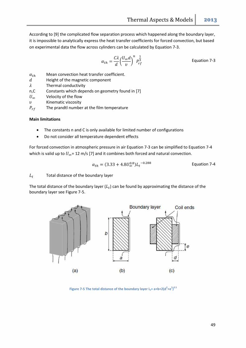
Thermal Aspects & Models 2013
49
According to [9] the complicated flow separation process which happened along the boundary layer,
it is impossible to analytically express the heat transfer coefficients for forced convection, but based
on experimental data the flow across cylinders can be calculated by Equation 7-3.
(
)
Equation 7-3
Mean convection heat transfer coefficient. Height of the magnetic component Thermal conductivity n,C Constants which depends on geometry found in [7] Velocity of the flow Kinematic viscosity The prandtl number at the film temperature
Main limitations
The constants n and C is only available for limited number of configurations
Do not consider all temperature dependent effects
For forced convection in atmospheric pressure in air Equation 7-3 can be simplified to Equation 7-4
which is valid up to = 12 m/s [7] and it combines both forced and natural convection.
Equation 7-4 Total distance of the boundary layer The total distance of the boundary layer ( ) can be found by approximating the distance of the boundary layer see Figure 7-5.
Figure 7-5 The total distance of the boundary layer Lt= a+b+2(d2+e
2)
0.5

Thermal Aspects & Models 2013
50
Natural convection can be expressed by Equation 7-5 [7].
(
)
(
)
Equation 7-5
Main limitations
The constants n and C is only available for limited number of configurations
The previous recommended models are not valid for temperatures above 400 K therefore a high
temperature model needs to be developed from scratch. The basic equations will is described in the
following equations see [1] for a more details.
The heat transfer models for natural convection that have been developed for circular toroid’s are
based on the general expression of convective heat transfer from isothermal three dimensional
bodies see Equation 7-11.
Equation 7-6
Kinematic viscosity Density of the cooling fluid Dynamic viscosity The prandtl number describes the ratio of momentum diffusivity to thermal diffusivity see Equation
7-7.
Equation 7-7
Pr Prandtl number Kinematic viscosity The constant pressure specific heat capacity
Thermal conductivity of the fluid
Equation 7-8
The thermal diffusivity Natural Convection
Convection by natural sources can be described by the Grashof number Equation 7-9 which describes
the ratio of internal driving force to a viscous force acting on the flow, this relationship is valid up to
Gr = 109 and the flow is turbulent for larger values.
Equation 7-9
Gr Grashof number The characteristic length Gravity constant

Thermal Aspects & Models 2013
51
The thermal volume expansion coefficient Difference between wall and bulk fluid temperature
The Rayleigh number Equation 7-10 is a dimensionless number associated with the heat transfer
within the fluid in natural convection.
Equation 7-10 Ra Rayleigh number Natural Convection on Vertical Surfaces
The Nusselt number describes the improvement of heat transfer compared to a hypothetical static
fluid. The Nusselt number can be found by Equation 7-11 and Equation 7-12.
Vertical cylinders natural convection:
(
)
Equation 7-11
function Nusselt number
[ (
)
]
Equation 7-12
Horizontal cylinders natural convection:
(
)
Equation 7-13
[ (
)
]
Equation 7-14
Equation 7-15
Examples of he expected thermal conductivity in smaller toroid’s can be seen in Table 7-4 it can be
seen that the ambient temperature only have a minimal influence on the thermal conductivity,
however it is a small negative influence. This is possible due to the density of the air is decreasing.

Thermal Aspects & Models 2013
52
Table 7-4 Thermal conductivity examples
Core
C058583A2 = 13.62 = 12.42 ΔT = 86 = 13 = 11.72 ΔT = 88 C055089A2 = 10.98 = 10.31 ΔT = 91 = 10.23 = 9.54 ΔT = 93 0077715A7 = 11.23 = 10.02 ΔT = 86.92 = 10.47 = 9.2 ΔT = 88 Core C058583A2 = 11.38 = 10.3 ΔT = 51 = 10.84 = 9.73 ΔT = 52 C055089A2 = 9.0 = 8.44 ΔT = 33 = 8.45 = 7.85 ΔT = 34 0077715A7 = 9.24 = 8.2 ΔT = 31 = 8.69 = 7.57 ΔT = 32.6
Forced Convection
Forced convection happen when there is an external source of fluid flow that can be described by
Equation 7-17. This equation relates forced convection to Rayleigh number which is used instead of
the Nusselt number in Equation 7-15. The characteristic length L is different than in natural
convection since, this is the boundary the fluid move along on its path around the component, and
has to be calculated based on the actual fluid movement.
Equation 7-16
Reynolds number w Fluid velocity Equation 7-17 Rayleigh number
The previous equations require experimental data which have been found and are located in Table
7-5 for air and oil, T is evaluated at the point halfway between ambient and surface temperature.
Table 7-5 Thermal properties of Air and Oil [8] T in Celcius
Air 1.225 273/(T+258) [Kg m-3]
β 1/(T+273) [K-1] 16.8 10-6+52 10-9 T [Kg m-1 s-1] λ 0.0242+6.2 10-5 T [W m-1 -1] 1000 [J kg-1 K-1]
Oil 887-0.659 T [Kg m-3] β 8.6 10-4 [K-1] 0.13573 10-5exp(2797.3/(T)+273) [Kg m-1 s-1 ] λ 0.124-1.525 10-4 T [W m-1 -1] 1960+4.005 T [J kg-1 K-1]

Thermal Aspects & Models 2013
53
Heat transfer by radiation 7.7
The energy transmitted to the surroundings by electromagnetic waves is called radiation, and is both
small compared to other mechanisms and demanding to model [5]. The heat transfer by radiation
can be estimated by Stefan-Boltzmans law see Equation 7-18 [4]. is the radiated power, E is
emissivity of the surface is the surface temperature , the ambient temperature and A is the
effective surface area.
Equation 7-18
ε Emissivity Effective core area
The emissivity of some surfaces have been investigated and listed in Table 7-6 these values can be
used to calculate the thermal dissipation from radiation. Using the value for ferrites the radiated
power for some temperatures are given in Table 7-7., it can be seen that at the extreme case with
the ambient temperature of 250°C and ΔT of 100°C the power dissipation ability has increase nearly
fivefold.
Table 7-6 Emissivity of some surfaces [7]
Material Temperature Emissivity [-]
Aluminium polished (T = 100°C) 0.04 Ferrites (T = 100°C) 0.95 Copper polished (T = 100°C) 0.052 Isolation paper (T = 100°C) 0.9 Enamel (T = 100°C) 0.9 Enamel Copper (T = 100°C) 0.9 Typical Transformer Na 0.58 [9]
Table 7-7 Radiation at different temperatures
Case E Rθ
Close to normal temperature 0.9 293 393 845.6 A 0.118/
Elevated temperature 0.9 418 518 2245.5 A 0.045/
Extreme temperature 0.9 518 618 4000 A 0.025/
The heat transfer from radiation depends on the surface area which is able to radiate energy away
from the component. This means that the effective surface (enveloped surface) is smaller than the
real surface area, the enveloped surface includes all vertical parts but in areas where the radiation
from two surfaces will interact with each other the radiation will be lower than the sum of the
surfaces and this can be approximated by the Pythagorean theorem.
The effective surface area for toroid’s can be calculated with Equation 7-19 and Equation 7-20 [10]
√
Equation 7-19
F View factor

Thermal Aspects & Models 2013
54
Core outer diameter including wire Core inner diameter including wire Core height including wire
(
) Equation 7-20
The equations describing the heat transfer from radiation is not easy to experimentally verify due to
convective heat transfer, but a COMSOL model was created based on the KoolMμ sample described
in Table 10-1 with 10 W of internal power generated and an emissive coefficient of 0.5 to compare
the different ways to calculate the effective surface area. COMSOL do not use the effective surface
area Equation 7-20. The deviation in surface area between the two formulas for the mentioned
model is only 6.71 %.
Figure 7-6 COMSOL model of a core including only radiation
Mounting 7.8
There are primarily 6 different ways a toroid core can be mounted to a PCB and located in space and
this can have allot to say for the cooling efficiency, however the cooling options might be limited due
to space issues. The different options are:
Vertical mounted core on a vertical PCB this option lets air pass through the component
increasing cooling and more space

Thermal Aspects & Models 2013
55
Horizontal mounted core on a vertical PCB this do not let air pass through the core reducing
the cooling efficiency, however a small air gap can be created between the PCB and core to
increase the cooling.
The two previous options under the PCB.
The two first options just on a vertical PCB. It is likely that this have the overall best cooling
efficiency.
Depending on previous described cases the characteristic length changes and have to be calculated
for each case, and which surfaces that a vertical and horizontal changes which have to be taken into
account in any model. In Figure 7-7 vertical and horizontal mounted cores are shown.
Figure 7-7 Horizontal and vertical mounted cores
Empirical thermal model 7.9
The temperature rise of an inductor core can be estimated by a best fit curve based on empirical data
[6] which has been shown to have an error of less than five percent [2]. This approach is
recommended from several magnetic core manufactures but do not take into account other cooling
options than natural convection with air.
(
)
Equation 7-21
Power loss W Surface area including the windings m2

Thermal Aspects & Models 2013
56
Main limitations
Do not consider ambient temperature
Do not consider forced convection or heat sinks
Do not consider geometry or how the core is mounted
Only available for air
Model comparison 7.10
The different thermal models have been compared to a COMSOL model of the same core in
Table 7-9. The model includes that all surface areas radiates energy, and natural convection is in
effect. The model data can be seen in Table 7-8. The measured values were performed by driving a
large 50 Hz current through a core with 16 turns of Litz wire. The COMSOL model do not take into
account the increase of surface area due to the windings, while empirical model assumes that the
whole surface area is covered which means that it would overestimate the temperature by a small
bit, if the core was fully covered in turns. It can be observed that analytical model overestimates the
temperature by a large factor and therefore the empirical model should be used. This problem was
not discovered due to some parameters which was wrong leading to very good results in the tested
cases. The problem is most likely related to the calculation of surface area since both the COMSOL
model and analytical model have problems.
Table 7-8 COMSOL model data for C058583A2
Variable Value Unit Description
Od 51.7 [mm] Outer diameter Id 30.9 [mm] Inner diameter Ht 14.4 [mm] Height ε 0.58 [-] Emissivity
Table 7-9 Comparison of temperature increase in C058583A2 for natural convection
Power [W] COMSOL [°C]
Analytical [°C]
Empirical [°C]
Measured Values [°C]
10 95.65 98 42.83 56.7 3 36.10 22 15.71 21.3 1 14.41 17.3 6.29 9.6
A second sample was prepared with 106 turns of Litz wire on a C058583A2 to see how the models
perform on a core with windings, it can be seen that the COMSOL model is do not manage to predict
the losses accurate in the way it is designed. However as the temperature increases the analytical
model outperforms the empirical model.

Thermal Aspects & Models 2013
57
Table 7-10 C058583A2 including windings
Variable Value Unit Description
Od 39 [mm] Outer diameter Id 11 [mm] Inner diameter Ht 16 [mm] Height ε 0.58 [-] Emissivity
Table 7-11 Temperature comparison in C058548A2 with 106 turns of 120 x 0.1 Litz wires with natural convection cooling
Power [W] COMSOL [°C]
Analytical [°C]
Empirical [°C]
Measured Values [°C]
10 121 117 83.71 91 3 46.7 48 30.7 30 1 18 12.57 12.29 17.35
The 106 turns C058583A2 test was repeated at 100 °C ambient temperature, and the results can be
seen in Table 7-12. However to keep a stable ambient temperature at 100 °C is complicated
especially since forced convention is necessary to increase the temperature in the heating chamber,
and very low accuracy in the measured values is to be expected. It can be seen that the core
increases in temperature in comparison to the ambient for the COMSOL model this could be due to
convective cooling is reduced at higher temperature, due to lower air density or other factors.
Table 7-12 Temperature comparison in C058548A2 with 106 turns of 120 x 0.1 Litz wires with natural convection cooling at 100 °C ambient temperature
Power [W] COMSOL [°C]
Analytical [°C]
Empirical [°C]
Measured Values [°C]
10 197.04 164 183.71 157.87 10 197.04 164 183.71 148.5 3 156.18 139 130.7 112.5 3 156.18 139 130.7 117
Winding thermal resistance 7.11
The thermal resistance of a single layer winding is according to [11] in the range from 0.6 to 1.5 Wm-
1K-1 at a fill factor of 0.5. In a multilayer design like a Litz wire COMSOL modeling of the problem
shows that the thermal conductivity for multilayer design is close to that of a single layer. By varying
the copper area and insulation the thermal conductivity at different fill factors was obtained [11] see
Figure 7-12.
This model do not consider the heat generation within the windings therefore the model in [11] was
replicated in COMSOL with 50% of the heat loss in the windings and 50% in the core see Table 7-13.
Rearranging Equation 7-1 yields Equation 7-22 to calculate the thermal conductivity.

Thermal Aspects & Models 2013
58
Equation 7-22
Length from the heat source to the boundary Width of material d Depth of material
Table 7-13 COMSOL model data for the windings
Variable Value Unit Description
401 [Wm-1K-1] Thermal conduction in copper 0.5 [Wm-1K-1] Thermal conduction in insulation 0.03 [Wm-1K-1] Thermal conduction in air 5 [W] Heat source in the core 5 [W] Heat source distributed evenly in the layers 2 10-4 [m] Insulation thickness 2 10-6 [m2] Copper wire cross section in each layer Fill factor 0.5 [-]
The Thermal conductivity in the cases where the losses in the windings equals those in the core
increases to 0.76 Wm-1K-1. However with two layers decreases to 0.727, three layers 0.6816 and
10 layers 0.699 see Figure 7-8 - Figure 7-11. In practice it is nearly impossible especially in toroid’s to
have a perfect winding pattern so these values should be used as a maximum for the thermal
coefficient. A simulation with-non ideal winding configuration can be seen in Figure 7-13 decreasing
from 0.6816 to 0.273, somewhere between these values is the likely true heat conductivity for a
three layer design.
Figure 7-8 Heat conduction
in a single layer
Figure 7-9 Heat Conduction
in two layers
Figure 7-10 Heat
conduction in three layers
Figure 7-11 Heat
conduction in ten layers
The fill factor in the winding section also affects the thermal conductivity and lower fill factor means
that more of the winding area is isolation and air, this have been plotted in Figure 7-12 for a single
layer.

Thermal Aspects & Models 2013
59
Figure 7-12 Thermal conductivity for different fill factors [11]
Figure 7-13 Heat conduction for non-ideal
windings
In Table 7-15 values for the thermal conductivity in 9 different cases have been listed depending on
where the loss is located and layers. These values will in the next chapter be used as a part of a
thermal model of magnetic components.
Table 7-14 Thermal conductivity for different configurations with 50 % fill factor
Layers Core loss 25% Core loss 50% Core loss 75%
1 0.91 0.76 0.65 2 0.9 0.75 0.64 3 0.82 0.681 0.58
10 0.84 0.7 0.6
Core thermal resistance 7.12
The thermal conductivity of different magnetic materials is listed in Table 4-1 - Table 4-2 and can be
used to calculate the thermal resistance of the core. For an uncoated core this resistance is close to
zero and can be neglected, however in the case of powder cores, the epoxy coating have a much
lower thermal conductivity. An approximate value for this can be found in Table 7-3 where epoxy
resins have a thermal conductivity of 0.25 K W-1. A simple Comsol model reveals that the core
thermal resistance can still be neglected see Figure 7-14 and Figure 7-15.
The model was created by a 2D equivalent of the core with 293.15°C boundary condition on the
outer surfaces, and a heat source covering the inner area see Table 7-15 for the other constraints.
Table 7-15 COMSOL model data for core thermal resistance
Variable Value Unit Description
Od 51.7 [mm] Outer diameter Id 30.9 [mm] Inner diameter Ht 14.4 [mm] Height 8 [Wm-1K-1] Thermal conduction in the core 0.25 [Wm-1K-1] Thermal conduction in epoxy 5 [W] Heat source in the core 0.5 [mm] Insulation thickness

Thermal Aspects & Models 2013
60
Figure 7-14 Heat conduction in the core with dins= 0.5 mm
Figure 7-15 Heat conduction in the core with dins= 2 mm
Thermal model for toroid magnetic components 7.13
The temperature increase of an inductor can be modeled by an analytical model which depends on
the actual configuration of the magnetic material. The designs which implanted into the magnetic
design software are toroid cores and other cores with the windings fully exposed to the environment,
in cores with very high fill factor this is not correct however the model will be developed for the
general case. This lays the foundations for the model, and an equivalent circuit based analogy can be
made further explained in literature [4].
The thermal resistance between the maximum core temperature and the ambient can in an inductor
is split into these components:
Core thermal resistance ( ) is the thermal resistance between the core and windings, it is hard to
quantify due to that the thermal sources are evenly distributed through the magnetic material and
therefore depends greatly on geometry [3] however as shown in section 7.12 this resistance is so low
that it can be ignored for powder cores and ferrites due to the semi high thermal conductivity of the
material.
Winding thermal resistance ( ) is the thermal resistance from the core and to the surface of the
windings. The heat generated by the windings is distributed from the core and to the surface inside
each turn. Copper have a very low thermal resistance but due to the insulation is much higher
[3] see section 7.11.
External forced convection resistance this resistance describes the cooling from forced
convection on the surfaces facing the cooling stream, see section 7.6 for further details.
External natural convection for vertical surfaces resistance describes the cooling by
natural sources on vertical surfaces (section7.6).
External natural convection for horizontal surfaces resistance describes the cooling by
natural sources on horizontal surfaces.

Thermal Aspects & Models 2013
61
Sink or PCB resistance describes the heat transfer to the board the core is mounted on or to
other sources like a heat sink (section7.6).
Radiation resistance describes the cooling done by radiation (section 7.7).
The complete equivalent circuit for a toroid can be seen in Figure 7-16 describes core losses and
the winding losses however since is very low the winding and core losses can be put as a
single source simplifying the model.
Figure 7-16 Equivalent thermal circuit
Assumptions for the model
Toroid or similar shape
The core is fully covered with windings
The emissivity for the whole component is assumed to be 0.58 from Table 7-6
The windings thickness increases twice as much on the inner diameter compared to the
outer.
Pressure is not taken into account

Thermal Aspects & Models 2013
62
External thermal resistance 7.14
The external thermal resistance describes how easily the windings are cooled down.
Natural Convection
The external thermal resistance for natural convection is described by Equation 7-23 and Equation
7-24 see Appendix G for the derivation.
(
[
[ ( )
]
]
)
Equation
7-23
(
[
[ (
)
]
]
)
Equation
7-24
Radiation
(
) Equation 7-25
Inserting Equation 7-19, Equation 7-20 into Equation 7-18 gives the total heat loss from radiation
based on the dimensions of the core including the windings. However this results in a nonlinear
equation and is best to be solved by a computer. See Appendix G for example of the basic calculation
with some simplifications.

Thermal Aspects & Models 2013
63
References 7.15
[1] VDI Heat Atlas, Springer-Verlag Berlin 2010
[2] Zientarski, J.R.R.; Pinheiro, J.R.; Hey, H.L.; Beltrame, R.C.; Candido, D.B.; , "A design methodology for boost inductor applied to PFC converters considering the core temperature rise and the conducted EMI noise," Power Electronics and Applications, 2009. EPE '09. 13th European Conference on , vol., no., pp.1-10, 8-10 Sept. 2009
[3] Lloyd H. Dixon “Magnetic Design Handbook” Texas Instruments 2001 [4] N. Mohan and T. M. Undeland, Power Electroncis Converters, Applications, and Design:
John Wiley & sons, 2003. [5] Jonas Muhlethaler “Optimal Design of inductive components Based on Accurate Loss and
Thermal Models” 2012
[6] Magnetics® Technical Bulleting “Powder Core Catalog” 2011 [7] A. Bossche, V. Valchev Inductors and Transformers for Power Electronics 2005 [8] Villar, I.; Viscarret, U.; Etxeberria-Otadui, I.; Rufer, A.; , "Transient thermal model of a
medium frequency power transformer," Industrial Electronics, 2008. IECON 2008. 34th Annual Conference of IEEE , vol., no., pp.1033-1038, 10-13 Nov. 2008
[9] Coonrod, Neil R., "Transformer Computer Design Aid for Higher Frequency Switching Power Supplies," Power Electronics, IEEE Transactions on , vol.PE-1, no.4, pp.248,256, Oct. 1986
[10] Refai-Ahmed, G.; Yovanovich, M.M.; Cooper, D., "Heat transfer modeling of toroidal inductors: Effect of orientations," Thermal and Thermomechanical Phenomena in Electronic Systems, 1998. ITHERM '98. The Sixth Intersociety Conference on , vol., no., pp.417,423, 27-30 May 1998
[11] T. Nilsen and R. Lund memo “Calculation of thermal conductivity in a Litz wire bunch with COMSOL multiphysics” 2006
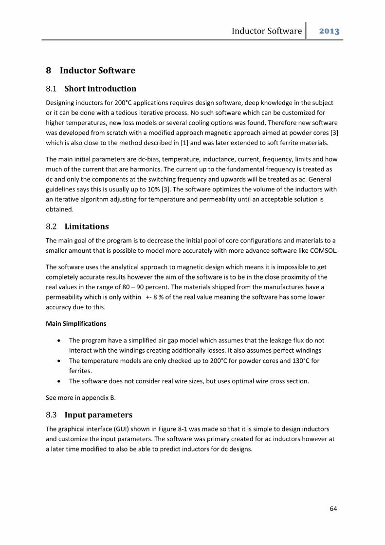
Inductor Software 2013
64
8 Inductor Software
Short introduction 8.1
Designing inductors for 200°C applications requires design software, deep knowledge in the subject
or it can be done with a tedious iterative process. No such software which can be customized for
higher temperatures, new loss models or several cooling options was found. Therefore new software
was developed from scratch with a modified approach magnetic approach aimed at powder cores [3]
which is also close to the method described in [1] and was later extended to soft ferrite materials.
The main initial parameters are dc-bias, temperature, inductance, current, frequency, limits and how
much of the current that are harmonics. The current up to the fundamental frequency is treated as
dc and only the components at the switching frequency and upwards will be treated as ac. General
guidelines says this is usually up to 10% [3]. The software optimizes the volume of the inductors with
an iterative algorithm adjusting for temperature and permeability until an acceptable solution is
obtained.
Limitations 8.2
The main goal of the program is to decrease the initial pool of core configurations and materials to a
smaller amount that is possible to model more accurately with more advance software like COMSOL.
The software uses the analytical approach to magnetic design which means it is impossible to get
completely accurate results however the aim of the software is to be in the close proximity of the
real values in the range of 80 – 90 percent. The materials shipped from the manufactures have a
permeability which is only within +- 8 % of the real value meaning the software has some lower
accuracy due to this.
Main Simplifications
The program have a simplified air gap model which assumes that the leakage flux do not
interact with the windings creating additionally losses. It also assumes perfect windings
The temperature models are only checked up to 200°C for powder cores and 130°C for
ferrites.
The software does not consider real wire sizes, but uses optimal wire cross section.
See more in appendix B.
Input parameters 8.3
The graphical interface (GUI) shown in Figure 8-1 was made so that it is simple to design inductors
and customize the input parameters. The software was primary created for ac inductors however at
a later time modified to also be able to predict inductors for dc designs.

Inductor Software 2013
65
Figure 8-1 GUI of the Inductor designer
Input parameters:
1. Dc Bias
Permeability has to be adjusted according to the magnetizing forces which mean value is
raised by the product of dc current and windings.
2. Ambient Temperature
This parameter is to adjust for the temperature of the surroundings which is used in
permeability calculations, thermal calculations and as a part of the temperature limit.
3. Temperature limit
Maximum temperature is the limiting value for core and winding losses and the inductor
have to stay below this limit. This value depends on what materials that is used and the
temperature limit of surrounding components. The included database has a temperature
limit of 200 degrees, but due to the simplifications in the analytical models the maximum
temperature should be used a guideline and not an absolute limit.
4. Peak Inductance
The inductance wanted at peak fundamental current adjusted for frequency, temperature,
current peak and dc bias.
5. Ripple peak value
The ripple peak current value which is used in the loss calculations.

Inductor Software 2013
66
6. Current Peak Value
The output current peak value which is used in the peak permeability calculations for a high
frequency filter with a fundamental current this would be the peak of the fundamental not
including dc bias.
7. Average output current
The average output current which is used to determine the losses.
8. Ripple Current
The percent ripple experienced at the switching frequency, a good approximation is at
around 10%, this is calculated from the current peak value.
9. Fundamental Frequency
This value should be set to the fundamental frequency of the load.
10. Switching Frequency
The high frequency losses are assumed to be around the switching frequency so this value should be set to the switching frequency of converter / inverter.
11. Current Density
The current density in the windings can be set with this option for a high frequency design this is often in the order of 200 Acm-2.
12. Maximum Fill Factor
The maximum copper fill factor is the product of windings and cross section of each
conductor divided by the window area. The recommended value is around 0.4 but in Litz wire
designs or for other reasons the fill factor can be raised.
13. Number Of Results
The results are sorted based on minimum volume and this option makes it possible to obtain
several different cores which satisfy the input parameters starting with the smallest core.
14. Minimum Number of Iterations
The minimum number of iterations is used to make sure that the design has actually reached
convergence and not just found a minor stable area. This value should be kept above 20.
15. Number Of Stacked Cores
In some cases it would be beneficial to stack several cores on top of each other resulting in a
smaller design this option give that possibility. All the relevant input core data is simply
multiplied with this factor.
16. Maximum Temperature Deviation
The large number of temperature dependent variables can lead to long computing time
however this option set how small the temperature deviation between iterations have to be
before the result is considered correct, however putting a very low value can lead to the
program getting stuck. To counter act this, a hard limit of 500 iterations was hardcoded
which will result in the core being ignored.

Inductor Software 2013
67
17. Maximum Number Of Winding Layers
Depending on how many turns the core needs to obtain the necessary inductance the
software approximates how many turns can fit into each winding layer this option put a limit
to how many layers there can be. The number of winding layers greatly affects the ac
resistance see section 6.1 and parasitic capacitances see section 6.5.
18. Maximum core height
In many designs the space is limited and this option will lead to all cores with a height larger than the input is ignored, however this only for the core material and with windings the inductor can become larger.
19. Maximum core diameter
In many designs the space is limited and this option will lead to all cores with a diameter larger than the input is ignored, however this only for the core material and with windings the inductor can become larger.
20. Maximum air gap
Ferrite materials needs an air gap store energy and to limit the flux however an increasing air gap leads to larger fringing flux which can induce currents in the windings or generate other problems. This option will set a limit to the length of the air gap.
21. Forced Convection
Natural convection is assumed for the thermal calculations if this option is not checked, if a value is entered this will describe the mean flow over the component.
22. Heat Sink
The unknown nature of the heat sink, pcb board or similar is impossible to predict generally therefore it is assumed that the thermal resistance to these elements are infinite however this option can be used to enter this resistance.
23. Thermal conductivity of the winding
The winding configuration can be too complicated to calculate the conductivity accurate especially in the case of Litz wire. The software approximate this value based on the number of layers and fill factor if no value is given see section 7.11 for more information and values.
24. Litz wire
In a high frequency design Litz wire may be necessary to reduce the winding losses see section 6.1 and 0. The initial program setup assumes normal windings so choosing this option leads the thermal calculations to use approximations to the heat transfer in Litz wire however the maximum fill factor has to be adjusted by the user. This option could also be used in cases where the wire size is known by setting strands to 1 and having strand diameter and bundle diameter equal to the wire size.
25. Number of strands in the bundle
Litz wire is built up by smaller wires here called strands this number is used to determine wire losses by increasing the layer variable by the number of layers there would be in a bundle.

Inductor Software 2013
68
26. Strand diameter
The diameter of the strand is used to determine the x coefficient in section 6.1 which describes the radius to skin depth.
27. Bundle diameter
The diameter of the bundle is used to calculate different parameters which are affected by the size of the windings.
28. Fast Thermal
The thermal calculations use a nonlinear solver which in some cases can increase the computing time. Choosing this option leads to a faster thermal calculations based on section 7.9 and will not consider forced convection, temperature or any other thermal related inputs.
29. Ferrite or Powder Cores
The program and its databases are built up around ferrites and powder cores. This check box
is used to either choose ferrite materials or powder cores. The option to run both in same
run was not implanted.
30. Core
In the cases where it would be beneficial to do calculations on a specific core, the part number can be entered here.
31. Run
This runs the program based on the input and outputs possible core sizes and configurations
in a excel file called Log.csv this file is located in the same folder as the software.

Inductor Software 2013
69
Output parameters 8.4
The results from running the program can be found in the files named Results_Powder.txt or
Results_Ferrite.txt in the programs folder. The output information provided can be viewed in Table
8-1.
Table 8-1 Output Parameters
Parameter Value
Core Data [-] All information provided by the manufacturer is provided here. H [ATcm-1] Magnetizing field used to calculate permeability and inductance. Bpeak Ripple [T] Peak value of the magnetic flux density. Al [nH N-2] Core nominal inductance adjusted for temperature, dc-bias, and
frequency. Turns [-] Number of turns necessary to obtain required inductance. Wire D [m] The diameter required of the wire. Copper loss [W] Losses in the wire. Core Loss [W] Losses in the magnetic material. Total Loss [W] The losses including core and copper loss Loss per volume [mWcm-3] The loss per volume in cases where this is above 100 mW cm-3
the design is likely loss limited. Core Temperature [°C] The surface temperature of the core due to losses. Temperature [°C] The total temperature of the core in Celsius. Wire-Area [m2] Cobber area in each wire. Current Density [Acm-2] Current density provided by the input parameters. Core [-] The power loss per unit volume. My Correction [-] The roll off in permeability. Fill factor [-] How much of the cross section of the core is filled with wires. Peak L [H] The calculated inductance on the peak value of the fundamental
waveform. Average L [H] The calculated inductance at zero crossing for the fundamental
waveform. Volume [mm-3] The volume of the core. Inverter Frequency [kHz] The switching frequency. Surface [m2] The surface area of the component used to calculate the
temperature gain. Winding Layers [-] The calculated number of layers in the design Al from leakage [nHN-2] Primary the added nominal inductance from leakage fields. Gap length [cm] In ferrite designs this describes the length of the gap. Fr ripple [-] This is the dowel factor Rac/Rdc Winding length [m] The analytical length of the wire
Experimental results 8.5
The software described in the previous sections was used to create 4 different samples where the
Temperature, permeability, turns, fill factor, and loss was compared to the analytical values see
chapter 10 for the lab setup and 11.2.1 for the results. Generally it was a good correlation between
the analytical values and the measured except for temperature.

Inductor Software 2013
70
References 8.6
[1] Lloyd H. Dixon “Magnetic Design Handbook” Texas Instruments 2001
[2] Magnetics® Technical Bulleting “Powder Core Catalog” 2011
[3] Dr. Richard Lund SmartMotor email correspondence 31.09.2012

Filter Dimensioning 2013
71
9 Filter Dimensions The most common way to control a switch mode power supply is with pulse width modulation where
constant switching frequency is used, output voltage is controlled by adjusting the duty cycle. The
resulting output waveform need to be filtered so that components are put under lower stress.
Filter for a Buck converter 9.1
The output voltage straight out from a buck converter Figure 9-1 have large dv/dt effects and at
times the instantaneous voltage will either be zero or as much as the input side, by using elements
which stores energy like inductors and capacitors the waveform will smoothen out. In the periods
where the switch is on the inductive elements charges due to a positive voltage, while in the off
periods the inductive element releases its energy while they discharges see Figure 9-2[1].
Figure 9-1 Buck converter [1] Figure 9-2 Buck converter in continues mode [1]
The buck converter can operate in continues mode which means that over a period not all the energy
from the inductive element is released leading to a waveform as show in Figure 9-2 or discontinues
mode which means that all the energy is discharged in the off period, and there will be some time
where the voltage in the circuit will be zero. The ripple in continues mode is reduced by larger
inductive elements or by using higher frequency, the voltage ripple is not improved directly by the
inductive elements but by capacitive.
The most basic equation for an inductor Equation 9-1 can be rearranged into Equation 9-2, which can
be used inductance for a maximum ripple current.
Equation 9-1
L Inductance Output voltage Current ripple
Equation 9-2
Time period the switch is off

Filter Dimensioning 2013
72
Assuming that the ripple component of flows in to the capacitor C. The capacitor delivers charge
when the ripple current is below average and the necessary capacitance can be calculated by
Equation 9-3 [2].
Equation 9-3
Switching period Capacitance
The filter capacitor will also lead to a voltage drop across the equivalent series resistor (ESR) and
therefore the ESR should be kept low [2]. The buck converter will be used to determine the accuracy
of the inductor software and in Table 9-1 filter specifications for some cases can be viewed see more
information in Appendix D section V where the filters are calculated, designed with the inductor
software and tested.
Table 9-1 Buck filter specifications
Buck filter specification
[V] F [kHz] D [A] [V] L [mH] C [µF] 30 10 0.5 1.2 0.4545 1.25 33
100 10 0.5 4 1.5152 1.25 33
30 10 0.5 0.6 0.2273 2.5 33 100 10 0.5 2 0.7576 2.5 33
30 10 0.5 0.4286 0.1623 3.5 33
100 10 0.5 1.428 0.54 3.5 33
30 5 0.5 0.66 0.5 4.5 33 100 5 0.5 2.22 1.68 4.5 33

Filter Dimensioning 2013
73
Sinus and dv/dt Filter 9.2
A sinus and dv/dt filter will be calculated for a SiC inverter based on the case information given in the
introduction repeated in Table 9-2. It is assumed the inverter uses PWM switching technique with
maximum modulation index of one.
Table 9-2 Drive specification
Drive Specification
Vdc 600 V S 3000 Va fsw Up to 100 kHz Tamb 150 °C
1 kV/µs
Where Vdc is the Dc-link voltage S is the apparant power delivered fsw is the switching frequency Tamb is the downhole ambient temperature
The maximum line to line voltage can be found using Equation 9-4, is the modulation index which
in this case will be set to 1, the worst case scenario before going into over modulation.
Equation 9-4
9.2.1 RLC Dv/dt Filter
A dv/dt filter for silicon carbide drives need to limit the dv/dt to minimum 1 kV/µs, how this is done is
closer explained in chapter 3. A simulation model of the circuit was developed in section 3.6 and the
filter values was calculated based on the equations in Table 3-3.
Table 9-3 Dv/dt filter values
Parameter Value
Phase Voltage
Phase Current Resonance frequency 377 658 Filter inductance 15.9 µH
Filter capacitance 201 nF
Filter resistance 35.58 Ω
The filter parameters was simulated with the RLC PSCAD model due to limitations with software only
a single 1 meter section of the cable could be simulated. see Figure 9-3 to Figure 9-7 for the circuit
topology and the waveforms recorded before and after the filter. From the simulation results the
three phase sinus filter improves the voltage and current waveform and keep the rise time in the
order of around 2 µs. The effect of leakage capatiance have not been included however this will lead
to more oscilations in the ciruit.

Filter Dimensioning 2013
74
Figure 9-3 Circuit topology of the RLC filter model
Figure 9-4 The voltage waveform before and after the filter
Figure 9-5 The voltage and current waveform before the
load
Figure 9-6 Zoomed in view of the voltage before and after
the filter
Figure 9-7 Zoomed in view of the voltage and current at
the load

Filter Dimensioning 2013
75
9.2.2 Sinus Filter
The purpose of a sinus filter is to create a nearly sinusoidal output waveform from the filter. The
calculations are performed in the appendix D sections VII, and the results for the sinus filter are
summarized in Table 9-4. The design process follows the equations in chapter 2 and using the
recommended starting value for Lf at 1% Pu with a switching frequency at 100 k[Hz]. The dampening
factor was set at 2.
Table 9-4 Sinus filter values
Parameter Value
Phase Voltage
Phase Current Base impedance Base inductance Resonance frequency Filter inductance
Filter capacitance
The filter parameters was simulated using the pscad model, however due to limitations with
software only a single 1 meter section of the cable could be simulated. From the simulation resutls
the three phase sinus filter improves the voltage and current waveform to nearly a sinusoidal.
Figure 9-8 Circuit topology of the Sinus filter model
Figure 9-9 The voltage at the load and current
Figure 9-10 Filtered and unfiltered line to line voltage

Filter Dimensioning 2013
76
Filter comparison 9.3
The RLC and Sinus filter, both improves the waveforms so this section will compare the size of the
two filters. The inductors were designed by the software in chapter 8 with the input parameters that
can be viewed in Table 9-5. The smallest volume inductor which can be used are shown in Table 9-6
however this do not include any volume increase due to the windings.
The temperature factor was disregarded due to the cores being so small that it is likely the
temperature models do not model them correctly and the software have not been verified on so
small cores. However if the component do keep this high temperature it can be solved by using a
heat sink or removing heat by the pcb board.
It can be seen that the RLC filter inductor can be made very small compared to the sinus filter, this is
both due to a much smaller inductance and smaller reduction in permeability due the few turns
which is necessary. The Sinus filter inductor will also have a much larger volume due to the windings.
Parallel connection and stacking several cores on top of each other were considered but did not lead
to a smaller design.
Table 9-5 Input parameters
Inductor 1 Inductor 2
Dc Bias 0 A 0 A Ambient temp. 25°C 25°C Peak inductance 1.43 mH 15.9 µH Current Peak 6.66 A 6.66A Average output Current 4.71 A 4.71 A
Ripple current 10 % 10 % Fundamental frequency 1 1 Switching frequency 100 000 Hz 100 000 Hz Current Density 200 200 Number of strands in bundle
120 120
Strand diameter 0.1 mm 0.1 mm
Bundle diameter 1.55 mm 1.55 mm
Table 9-6 Software recommendations
Inductor 1 Analytical prediction
Inductor 2 Analytical prediction
Core Data C055306A2 Core Data C058128A2 Linital 7.21 mH Linital 2.37 µH Lpeak 1.44 mH Lpeak 1.62 µH Turns 133 - Turns 17 -
Copper loss 0.07 W Copperloss 0.0027 W CoreLoss 11.28 W CoreLoss 0.103 W Total Loss 11.35 W Total Loss 0.106 W
Temperature 152 °C Temperature 33.94 °C MyCorrection 0.205 - MyCorrection 0.68 -
Fill factor 0.82 - Fill factor 0.54 - Volume 1800 mm3 Volume 244 mm3

Filter Dimensioning 2013
77
References 9.4
[1] N. Mohan and T. M. Undeland, Power Electroncis Converters, Applications, and Design: John Wiley & sons, 2003.
[2] Øyvind Holm Snefjellå, “Silicon Carbide Technologies for High Temperature Motor Drives”, Master thesis, June 2011.

Laboratory setup 2013
78
10 Laboratory Setup This chapter describes how the laboratory setups were done, what equipment that has been used
and some initial measurements and comparisons.
There were four different setups:
Core characterization with a BROCHAUS MPG 100D steel tester. The measurements which
was performed was core loss in powder and ferrite cores, in the frequency range from 5 kHz
to 10 kHz at 20°C, 108°C, and 180.5°C.
Core loss with a waveform generator and an amplifier at 5 kHz, 20 kHz 50 kHz and 100 kHz, at
20°C and 180°C.
Inductor characterization with a buck converter.
Impedance measurements with a network analyzer.
Samples 10.1
The magnetic material which was possible to acquire for the tests, and that can be used in high
temperature designs are listed in Table 10-1. These include four different powder cores and two
ferrites, everything is from Magnetics® except the N27 which is produced by Siemens.
Table 10-1 Core materials
µ B [T] Al [nH/N2] Ve [mm3] Ae [mm2] le [mm] H [mm] Material
C058583A2 160 1.5 101 4150 46.4 89.5 9.78 High Flux C058548A2 125 1.5 127 5340 65.6 81.4 11.5 High Flux C055089A2 125 0.75 178 15600 134 116 16.1 MPP 0077715A7 125 1.05 152 15900 125 127 14.4 KoolMμ ZR44916TC 2300 0.47 2710 15010 118 127 15.9 R N27 2000 0.5 5100 166250 625 308 25 N27
Core loss characterization 10.2
The analytical data on core parameters are usually only available for a limited temperature ranges,
and is also not necessary accurate, therefore core loss characterization was performed, at three
different temperatures 20°C, 108°C and 180.5°C.
10.2.1 Measurement setup BROCHAUS MPG
The core characterization was performed with a BROCHAUS MPG 100D which is used to define the
magnetic qualities of electric sheets, and other magnetic materials. The rated measurement range is
from 3 Hz to 10 kHz [2] for toroid geometries with an inner diameter larger than 26 mm [2]. U core
geometries are not directly supported but can be transformed into an equivalent toroid core [3].
The measurements are performed electrically by a primary winding which creates a magnetic field
based on the input parameters. Voltage is measured over a precision resistor (shunt) in the
secondary winding which is unaffected by temperature and induced fields. Two separate systems
measure the values of B and H simultaneous avoiding errors due to phase differences [2], however
during the characterization of powder cores it was discovered that phase problems still might apply

Laboratory setup 2013
79
for long wires or different lengths of the primary and secondary winding. A flow chart over the
system can be seen in Figure 10-1.
Figure 10-1 Control principle for electric sheet measuring instrument [2]
The high temperature measurements were performed by increasing the ambient temperature to the
desired value with a heating chamber see Figure 10-2. It was assumed that the low losses induced in
the materials from the measurements would not significantly alter the core temperature, and the
heating chamber was set at forced convection meaning that if the core should increase in
temperature, it would be rapidly cooled down. The samples were heated up to the required
temperature for a minimum of four hours before the measurements began, which for materials with
thermal conductivity of 8 (see Table 4-2) is more than enough to get a uniform temperature in the
material. The secondary and primary winding was connected to BROCHAUS MPG by having 30 cm
long wires going out of the heating chamber and into, the plugin system see Figure 10-3. The
equipment that was used can be viewed in Table 10-2.
Table 10-2 Lab equipment
Application Equipment Product number
Temperature measurements Temp. measurer FLUKE 51:2 Adjusting the ambient temperature Heating chamber TERMAKS TS 8056

Laboratory setup 2013
80
Figure 10-2 The heating chamber rated for 0°C to 200°C
Figure 10-3 The plugin system for ring cores in BROCHAUS
MPG 100D
Samples
Details on the samples prepared for the core characterization can be found in Table 10-3. A primary
winding with 8 turns is used to magnetize the core in the range from 4 mT to 106 mT for powder
cores. This low range was chosen due to constraints in the Brochause measurement setup, however
the ripple flux which will be inducing the core losses in real applications are not likely to be much
larger. The secondary winding is set to be 8 turns with the same length as the primary to avoid phase
problems. [2] recommends five turns on both primary and secondary this was disregarded due to the
small increase in windings raised the induced flux to a more appropriate level and [2] is most likely a
recommendation for high permeability materials. The heating chambers maximum temperature was
measured to 180.5 °C when the settings was set to 200 °C and 108 °C with settings at 120 °C.
Table 10-3 Core loss samples
Picture
Pri
mar
y w
ind
ings
Seco
nd
ary
win
din
gs Description
8 8 A single 0077715A7 core wound with 8 turns of 120 x 0.1 mm Litz wire with a theoretical peak flux of 98 mT at 10 A. The purpose: of this sample is to test the core losses in koolMμ materials
8 8 A single C058583A2 core wound with 8 turns of 120 x 0.1 mm Litz wire with a theoretical peak flux of 179 mT at 10 A. The purpose: of this sample is to test the core losses in HighFlux materials

Laboratory setup 2013
81
8 8 A single C058548A2 core wound with 8 turns of 120 x 0.1 mm Litz wire with a theoretical peak flux of 154 mT at 10 A. The purpose: of this sample is to test the core losses in HighFlux materials
8 8 A single C055089A2 core wound with 8 turns of 120 x 0.1 mm Litz wire with a theoretical peak flux of 108 mT at 10 A. The purpose: of this sample is to test the core losses in MPP materials
6 6 A single ZR44916TC core wound with 6 turns of 30 x 0.1 mm Litz wire with a theoretical peak flux of 1360 mT at 10 A. The purpose: of this sample is to test the core losses for an R material ferrite with no air gap.
8 4 A double N27 U core core wound with 8 turns of 30 x 0.1 mm Litz wire with a theoretical peak flux of 650 mT at 10 [A]. The purpose: of this sample is to test the core losses for a N27 material ferrite with no air gap.
10.2.2 Core characterisation at 180.5°C
The Litz wire used in the measurements are rated for 130°C but as shown in section 0 deterioration is
not expected at 200°C for short term exposure, however in the case of short circuit in the winding, a
change in resistivity is to be expected. Therefore the resistance in both the primary and the
secondary winding was measured before and after the high temperature tests. This can be viewed in
Table 10-4. There were no large deviations in the measured results meaning it is highly unlikely that
any damage happened. However two samples not shown here had to be redone due to winding
failure.
Table 10-4 Winding resistance before and after the high temperature tests
Sample number
Material Rel. Perm. Primary winding 20°C
Secondary winding 20°C
Primary winding after 180.5°C
Secondary winding after 180.5°C
1 High Flux High Flux
160 16.74 mΩ 16.68 mΩ 16.75 mΩ 16.70 mΩ 2 125 18.01 mΩ 18.10 mΩ 18.02 mΩ 18.16 mΩ 3 KoolMµ 125 18.10 mΩ 18.21 mΩ 18.16 mΩ 18.29 mΩ 4 MPP 125 21.36 mΩ 19.80 mΩ 20.28 mΩ 19.94 mΩ 5 N27 2000 27.60 mΩ 27.87 mΩ 27.82 mΩ 27.14 mΩ 6 R 2300 09.60 mΩ 18.90 mΩ 09.56 mΩ 18.76 mΩ

Laboratory setup 2013
82
100 kHz measurements 10.3
The BROCHAUSE steel tester had a secondary system for measurements above 10 kHz however it
was not possible to get this operational within the time frame of this master thesis. Therefore
another setup was made by using a signal generator which could create high frequency, non-
sinusoidal and fundamental. The problem with using a function generator is that it can only supply
low current, and therefore a 100 kHz amplifier was connected in series amplifying the signal to a
maximum of 7.5 Arms with maximum voltage output of 40 Vpp. An Oscilloscope was connected over
the test object measuring voltage and current while a power analyzer module automatically
calculated the power using all available data points (2500). At measurements lower than 20 kHz a
high accuracy power meter was connected to the system see Table 10-5 for the complete equipment
list. This setup is consistent with the setup used in [5].
Table 10-5 Lab equipment for 100 kHz
Application Equipment Product number
Signal generation Signal generator WAVETEK 187 Signal amplification up to 7.5 A 100 kHz 4-quadrant amplifier Toellner TOE 7610-20 Current measurement Current probe TEKTRONIX P6021 Voltage measurement Voltage probe TEKTRONIX P5200A Power measurements < 20 kHz Power meter YOKOGAWA 2533E43 Power measurements Oscilloscope TEKTRONIX TPS 2014 Oscilloscope power application Power application TEKTRONIX TPS2OWR1 Signal summation Custom made - 50 Hz signal 12 VRms Custom made - Temperature measurements Data logger AGILENT 34972A
10.3.1 Core Loss measurements
The core losses was measured up to 100 kHz with the amplifier setup, however it is not likely these
results is as accurate as the loss measurements from the Brochause. The current probe was
calibrated until the error was less than 0.5 % at 5 kHz and the voltage probe to 1 %, however due to
the large inductive load, the error in the measurements can be significantly higher and it was not
possible to calibrate the probes for higher frequencies.
The flux density in the core material was found by measuring the voltage in a secondary winding and
using Equation 10-1 see Table 10-6 for the relevant waveforms.
∫
Equation 10-1
Table 10-6 Equations to calculate the flux density in the core
Waveform Equation
Sinus wave
Square wave
Triangular wave

Laboratory setup 2013
83
The secondary winding has a small voltage drop, but very low current flow in these wires. To avoid
phase angle problems the winding length was set to the same length as the primary. The wire losses
was minimized by using Litz wire of 240 x Φ 0.1 which is several times smaller than the penetration
depth at 100 kHz which means that the winding losses should be very close to the dc value.
Therefore the dc losses in the windings was measured and subtracted from the measured values at
higher frequencies, this is a small source of error but should not influence the overall results.
The amplifiers low output voltage for 100 kHz tests was counteracted by maximizing the flux density
in the core by lowering the number of turns, and keeping the output current at around 7.5 Arms, with
the voltage at 20 Vpeak see below for an example with 0077715A7 (KoolMµ) at 100 kHz. This shows
that the maximum flux density that can be tested at 100 kHz is 52 mT with 4 turns. This might seem
like a small number but in a real application the ripple wave should normally not very large.
√ [H]
√
= 4.44 turns
√
To validate the setup, values from the Brochause were compared to the measurements with the
amplifier see Figure 10-4 and Figure 10-5. It can be seen that the accuracy of the amplifier
measurements is not very compared to the Brochause however at 5 kHz the winding losses equals
around 90 - 95 % of the measured loss meaning a very small measurement error would yield results
that deviate strongly from the expected result. At higher frequency this error decreases since most of
the losses is located in the core. The test frequency was set to 5 kHz due to large deviations in the
measurements in the Brochause for frequencies near 10 kHz.
Figure 10-4 Measured loss in High Flux at 5 kHz
Figure 10-5 Measured loss in KoolMµ at 5 kHz
For the measurements between 5 kHz and 20 kHz a high accuracy power meter was also used however due to the very inductive load it is likely these measurements is not as accurate as the scope measurements. The accuracy of oscilloscope measurements at 100 kHz need to be very exact due to in for example a 90 VA coil operating at 100 kHz with 4 W of losses and a necessary accuracy of 0.4W would require an angle accuracy of 0.00444 rad. This translates to a time accuracy of 7.06 ns.

Laboratory setup 2013
84
The TEKTRONIX TPS 2014 have a time accuracy of 5 ns and therefore the error is 0.00629 rad at 100 kHz which translates into 0.62 W at 100 VA. This is the maximum error that can happen since measured cores had smaller VA than this at 100 kHz. At high frequencies the Brochause or the accurate power meter could not be used to compare the measured values, due to this as extra security a temperature sensor was connected to the core. The temperature gain of the core is primary dependent on geometry, therefore by measuring the temperature and loss at 100 kHz and comparing it to a core with the same dc loss, it is possible to verify the results within a reasonable frame if the values are correct, however as seen in chapter 7.11 a bit lower temperature is to be expected in the dc measurements due to all loss is located in the windings which is better cooled than the core. Calometric measurements would have been better but due to the limited time it was not possible to set up.
10.3.2 Fundamental waveform with a high frequency ripple
The current waveform experienced by filters is normally a fundamental with a high frequency ripple
see chapter 3 and 5. The losses, temperature and inductance in a inductor experiencing such a
waveform was investigated by summing the signals from a signal generator and a secondary
waveform, taken directly from the grid due to voltage limitations with the signal generator which
could only generator 20Vpp while the amplifier which was connected in series needed 35 Vpp to
operate at maximum.
10.3.3 Non-sinusoidal losses
Chapter 5 describes non-sinusoidal losses and by using the signal generator and amplifier this
problem was planned to be investigated, however the error in the measurements was too large to
draw any concrete conclusions.
Measurements with a Buck Converter 10.4
The inductors designed in the previous chapters should be tested in real applications to determine
the leakage inductance, saturation and performance. A buck converter operating in continues mode
was set up in the lab see Figure 9-1 Buck converter [1] for the circuit topology and Table 10-7 for the
equipment that was used.
Table 10-7 Lab equipment Buck converter
Application Equipment Product number
Signal generation Signal generator WAVETEK 187 Adjustable input voltage 3-phase variac LUBECKE 3R54-22-H Dc voltage generation Dc-Link GOSSEN Buck converter switch Converter Custom by NTNU Adjustable resistance Resistance RUSHTRAT Filter Capacitor 33µ B25832-A4336-K009 Filter Inductor Custom Power measurements Power meter YOKOGAWA 2533E43 Power measurements Oscilloscope TEKTRONIX TPS 2014 Oscilloscope power application Power application TEKTRONIX TPS2OWR1 Voltage measurement Voltage probe TEKTRONIX P5200A Current measurement Current probe FLUKE 80i-110s Temperature measurements Data logger AGILENT 34972A

Laboratory setup 2013
85
A Variac was connected to the main supply to give a variable voltage to the dc-link which feed the
converter. The core under testing was mounted horizontal thereby reducing the heat loss in one
direction. A capacitor of 33µ was connected from the inductor to the negative voltage of the
converter, and the resistive load connected from the inductor to the negative side.
The power losses voltage and current waveform was measured by an oscilloscope and a power
meter. Surface temperature was measured by a nonmagnetic thermocouple of T-type. The sensor
was attached by covering it with a bit of the winding, so this could lead to a small error however the
sensor itself had a tolerance of around 0.5°C up to 125°C.
Inductors was designed based on the four cases described in the buck filter section see section 9.1
and Table 9-1. See section 11.2 for the results and more details can be found in appendix D section V.
Table 10-8 Inductance and resistivity measurements in some inductors
Sam
ple
Nr.
Mat
eri
al
Rel
. P
erm
eab
il
ity
Turns Primary Secondary
Resistance mΩ Primary Secondary
Inductance mH Primary Secondary
KoolMµ 125 50 50 50.44 57.16 0.421 0.45 HighFlux 160 85 85 56 77.35 0.804 0.8 HighFlux 160 110 110 138.25 138.7 1.47 1.38 HighFlux 125 106 - 97.54 - 1.909 HighFlux 160 50 - 37.78 - 0.355 HighFlux 160 50 - 39.49 - 0.387
Leakage capacitance 10.5
The leakage capacitance of the magnetic cores was measured in cooperation with Amir Hayati Soloot
and the equipment in Table 10-9 which measures the impedance from 4 Hz to 30 MHz. This was then
used to calculate the leakage capacitance.
Table 10-9 Lab equipment for Leakage capacitance
Application Equipment Product number
Impedance measurement Network analyzer AGILENT E5061B
The leakage capacitance can be calculated by Equation 10-2 when the self-resonance frequency and
inductance is known.
Equation 10-2
The inductance in powder cores is not constant above a few hundred kilohertz therefore the
inductance at the resonance frequency is different from values measured at low frequency. This is a
problem since it was hard to measure the inductance at higher frequency with the available
equipment. Therefore the inductance measured at 10 kHz was adjusted by the analytical data
provided by the manufacturer, however this lowers the accuracy of the results. No better solution
was found in time and most of the larger cores have a low self-resonance frequency. The analytical

Laboratory setup 2013
86
data that was used can be viewed in [6], and some initial measurements can be viewed in Table
10-10 and Figure 10-6 - Figure 10-9, while the main results will be covered in the next chapter.
Table 10-10 Leakage capacitance and SRF in some different inductors
Turns Type Inductance at 10 kHz
Self-resonance frequency
Adjusted Inductance
Leakage capacitance
165 KoolMµ
Litz 120 strand 5.5 mH 97.14 kHz 5.5 mH 488 pF
136 High Flux 160µ
Enamel 3.0 mH 280 kHz 2.94 mH 107.6 pF
41 KoolMµ
Litz 120 strand 0.242 mH 670 kHz 0.235 mH 240 pF
16 KoolMµ
Litz 240 strand 35 µH 2.29 MHz 31.5 µH 153 pF
Figure 10-6 Impedance plot for 16 Turns Litz wire 240
strands
Figure 10-7 Impedance plot for KoolMµ 41 Turns Litz wire
120 strands
Figure 10-8 Impedance plot for 136 Turns enamel
Figure 10-9 Impedance plot for 165 Turns Litz 120 strands
103
104
105
106
107
108
-20
-10
0
10
20
30
40
50
60
70
X: 2.254e+06
Y: 64.82
103
104
105
106
107
108
0
10
20
30
40
50
60
70
80
X: 6.755e+05
Y: 77.39
103
104
105
106
107
108
20
30
40
50
60
70
80
90
X: 2.825e+05
Y: 85.46
103
104
105
106
107
108
20
30
40
50
60
70
80
90
100
X: 9.645e+04
Y: 98.44

Laboratory setup 2013
87
References 10.6
[1] N. Mohan and T. M. Undeland, “Power Electroncis Converters, Applications, and Design”: John Wiley & sons, 2003.
[2] “BROCHAUS MPG100 USER MANUAL” 2001
[3] Discussion with Arne Nysveen
[4] Discussion with Edris Agheb
[5] Christopher G. Oliver “Measurement and Modeling of Core Loss in Powder Core Materials Core Loss in Powder Core Materials” 2012
[6] Magnetics® Technical Bulleting “Powder Core Catalog” 2012

Measurements and Discussion 2013
88
11 Measurements and Discussion In the previous chapter the main points of the measurement setup and error sources was discussed,
in this chapter the focus will be on the results. The raw data from the measurements is located in
appendix D however the Brochause data was too large to be included and can be found in the DAIM
database.
Core loss 11.1
The core loss in N27, R-ferrite, High Flux, MPP, and KoolMµ was measured at different temperature
levels 20°C 108°C and 180.5°C for the frequencies 3 kHz, 5 kHz, 7 kHz and 9 kHz with a Brochause
steel tester. An amplifier was used to measure core losses at 5 kHz, 20 kHz, 50 kHz, and 100 kHz for
the temperatures 22°C and 180°C. From core loss theory the losses is not expected to abruptly
change several magnitudes however this is the case in some of the Brochause measurements, the
cause is likely an automatic system in the measurement equipment which changed the control
method between controlling H and B.
The analytical loss data was provided by the manufacturer [1] for the powder cores see Equation
11-1- Equation 11-4. Based on this the lowest losses is expected in MPP and the largest in High Flux
160, it can also be seen that the losses nearly double by using High Flux 160 over High Flux 125. Note
that the losses increase with higher permeability should not be used as a rule since in other materials
the losses can decrease by increasing the permeability.
MPP 125µ Equation 11-1
HighFlux 125 Equation 11-2
High Flux 160 Equation 11-3
KoolMµ 125 Equation 11-4
11.1.1 Core loss in KoolMµ 5 kHz – 9 kHz
The core loss measured in KoolMµ with the Brochause setup can be viewed in Figure 11-1 - Figure 11-4. The analytical data underestimates the core losses severely at all frequencies. One explanation for this could be the large variation between the samples since the manufacturer only promises that each core is within 8% of the promised permeability value. A sample with 8% lower permeability than the rated should consist of 8% more air/binder and
Figure 11-1 Measured loss in KoolMµ at 3 kHz

Measurements and Discussion 2013
89
therefore might have different losses. To test this idea the permeability was measured which resulted in a relative permeability of 143, this could explain a bit of the large difference. No analytical data for higher permeability KoolMµ cores were available, however lower permeability cores have nearly twice as high losses as the 125µ core at 5 kHz and 100mT.
Figure 11-2 Measured loss in KoolMµ at 5 kHz
Another possibility would be that the loss measurements are wrong or performed in a different manner than the background data for the analytical data, and the analytical data is based on the Steinmetz equation which in some cases can underestimate or overestimate the losses. However as it can be seen in Figure 11-5 where the losses have been measured with the amplifier setup there is not a large deviation between the two setups. The losses measured at 7 kHz is most likely only valid up to 70 mT and the 10 kHz measurements do not seem to have become stable even if the data is the mean of several measurements. The temperature do not affect the losses in any great extent up to 180°C however a 5 -10 % increase in loss is indicated which primarily happens in the temperature range from 108°C to 180°C. For temperatures below 108°C there is no significant deviation due to temperature.
Figure 11-3 Measured loss in KoolMµ at 7 kHz
Figure 11-4 Measured loss in KoolMµ at 10 kHz

Measurements and Discussion 2013
90
11.1.2 Core loss in KoolMµ 5 kHz – 100 kHz
The losses in KoolMµ between 5 kHz and 100 kHz were found using the amplifier setup described in
the previous chapter see Figure 11-5 to Figure 11-8 for the graphical representation of loss versus
flux density. The correlation between the Brochause and the amplifier at 5 kHz is good bellow 50 mT
but the amplifier measurers somewhat lower losses at 75 mT. This is to be expected since it can be
seen in Figure 11-2 that there have been a discontinues jump in losses at 60 mT. The measurements
was performed twice, however in the cases where there was a large variation between the two
measurements more measurements was performed. Initially 5 measurements at each point were
planned but due to the very low variation between the samples this did not seem necessary
especially due to long time each measurement took.
The analytical data underestimates the losses for all frequencies measured with a factor of 200 – 300
%. The temperature has a similar influence at 100 kHz as at 5 kHz.
The measurements at 50 and 100 kHz was not possible to perform in the full flux density range due
to constraints in the equipment, and the losses at 100 kHz is so low that the error from measuring
the angle between real losses and reactive losses might seriously influence the values, therefore the
100 kHz losses should not be trusted.
Figure 11-5 Measured loss in KoolMµ at 5 kHz
Figure 11-6 Measured loss in KoolMµ at 20 kHz
Figure 11-7 Measured loss in KoolMµ at 50 kHz
Figure 11-8 Measured loss in KoolMµ at 100 kHz

Measurements and Discussion 2013
91
The measured values can be used to calculate new values for the Steinmetz equation which
determines the analytical data see Table 11-2. The new parameters have been plotted in Figure 11-9
and Figure 11-10. It can be seen that the accuracy of the Steinmetz equation can be increased by
measuring some points in the area of interest, however the values should not be extrapolated. In a
high temperature design this should be done close to the operation temperature.
Table 11-1 KoolMµ new Steinmetz parameters
Range k α β
5 kHz – 20 kHz 0.025 mT – 0.075 mT
31.73 1.8822 1.6731
20 kHz – 50 kHz 0.025 mT – 0.05mT
1135 1.17 2.2001
Figure 11-9 Comparison of new Steinmetz parameters for
5 - 20 kHz at 20 kHz
Figure 11-10 Comparison of new Steinmetz parameters for
20 - 50 kHz at 20 kHz

Measurements and Discussion 2013
92
11.1.3 Core loss in High Flux 160 5 kHz – 9.9 kHz
The core loss measured with the Brochause setup can be seen in Figure 11-11 to Figure 11-14. There is less discontinues data with the Brochause measurement equipment in testing the High Flux materials compared to the KoolMµ, this could be due to the material properties which make measurements easier to perform. However there is still some control problems which leads to discontinues data in some case especially at 9.9 kHz but this is very close to the maximum rating of the equipment. The relative permeability of the materials was measured to 150 which mean some loss differences are to be expected, however as in the previous section the losses are very much larger than what should be expected in the magnitude of up to 600 %.
Figure 11-11 Measured loss in HighFlux 160 at 3 kHz
The temperature does not affect the losses in any significant way up to 180°C except a loss reduction of some percent.
The measurement sample was quite small physically which means there is a larger expected error than in the other samples.
Figure 11-12 Measured loss in HighFlux 160 at 5 kHz
Figure 11-13 Measured loss in HighFlux 160 at 7 kHz
Figure 11-14 Measured loss in HighFlux 160 at 9.9 kHz

Measurements and Discussion 2013
93
11.1.4 Core loss in High Flux 160 5 kHz – 100 kHz
The high frequency measurements can be viewed in Figure 11-15 - Figure 11-18 it can be seen that
the analytical data match the measured values in a large extent up to 100 kHz. However there is a
large deviation between the values measured with the Brochause setup compared to the amplifier
this might indicate that the Brochause steel tester is not suited for measuring low permeability cores
with high accuracy, since the amplifier results is built upon 48 separate measurements making it
highly unlikely that so many point would fit the analytical data if measurement setup was not
somewhat accurate. The high flux material could be measured up to a larger flux density than the
previous and the losses are higher which increases the accuracy.
Figure 11-15 Measured loss in High Flux at 5 kHz
Figure 11-16 Measured loss in High Flux at 20 kHz
Figure 11-17 Measured loss in High Flux at 50 kHz
Figure 11-18 Measured loss in High Flux at 100 kHz

Measurements and Discussion 2013
94
11.1.5 Core loss in High Flux 125 5 kHz- 9.9 kHz
The losses in High Flux 125µ material can be viewed in Figure 11-19 to Figure 11-22 however the
losses above 80 mT should not be trusted since it can be seen that there is a discontinuity in the data,
as previously explained this is likely due to a change in the control system. The same relationships
between the temperature and losses as with High Flux 160 is present which results in a small
negative temperature coefficient in the losses with increasing temperature, at least up to 180°C.
Figure 11-19 Measured loss in HighFlux 125 at 3 kHz
Figure 11-20 Measured loss in HighFlux 125 at 5 kHz
Figure 11-21 Measured loss in HighFlux 125 at 7 kHz
Figure 11-22 Measured loss in HighFlux 125 at 9.9 kHz

Measurements and Discussion 2013
95
11.1.6 Core loss in MPP 5 kHz- 9 kHz
The MPP losses where complicated to measure and the Brochause were not able to get results above
5 kHz at 180°C see figure Figure 11-23 - Figure 11-26 for the measured values. It can been seen that
in MPP the losses are several magnitudes higher than the analytical data even if the relative
permeability is very close to the rated value of 125. The previous measurements and this one
indicated there are large differences among the cores in the magnitude of core loss in the same way
that the manufacturer does only guarantee that the permeability is within +- 8 %. In the
measurements there is no relevant increase in core loss by temperature from 3 kHz to 5 kHz however
there seem to be some problem in measuring loss at high temperature for higher frequencies but
this is likely to be related to the measurement equipment.
Figure 11-23 Measured loss in MPP 125 at 3 kHz
Figure 11-24 Measured loss in MPP 125 at 5 kHz
Figure 11-25 Measured loss in MPP 125 160 at 7 kHz
Figure 11-26 Measured loss in MPP 125 at 9.9 kHz
11.1.7 Core loss in MPP 5 kHz- 100 kHz
The loss in MPP was measured up to 100 kHz using the amplifier setup. However the loss which was
measured is not very large giving possibility of a large error. The low core loss means that the angle
between real loss and reactive loss become very important which was shown in section 10.3.1. This
should primarily be the case at 100 kHz but at 50 kHz the losses are allot lower meaning the error is
large in this case also. Some small relationships can however be found, that there is some close to no
increase in core losses with temperature.

Measurements and Discussion 2013
96
Figure 11-27 Measured loss in MPP at 5 kHz
Figure 11-28 Measured loss in MPP at 20 kHz
Figure 11-29 Measured loss in MPP at 50 kHz
Figure 11-30 Measured loss in MPP at 100 kHz
The measured values can be used to calculate new values for the Steinmetz equation which
determines the analytical data see Table 11-2. The new parameters have been plotted in Figure
11-31 and Figure 11-32. The MPP loss should be further investigated with a more accurate loss setup,
possible involving calometric measurements.
Table 11-2 MPP new Steinmetz parameters
Range k α β
5 kHz – 20 kHz 0.025 mT – 0.075 mT
33.24 1.74 1.66
20 kHz – 50 kHz 0.025 mT – 0.05mT
861.76 1.24 2.3

Measurements and Discussion 2013
97
Figure 11-31 Comparison of new Steinmetz parameters for
5 - 20 kHz at 20 kHz
Figure 11-32 Comparison of new Steinmetz parameters for
20 - 50 kHz at 20 kHz
11.1.8 Core loss in N27 Ferrite
A N27 ferrite core from EPCOS was measured with the Brochause steel tester, and the sample was
quite large compared to all other measured cores with a weight that was around 6 – 7 times higher
than any other samples. This reduces the measurement error, however it was a double U core which
was transferred to the equivalent toroid shape.
The measurement fit the analytical data very well, but the measured loss is lower than the
producer’s analytical data. This could be because the analytical data is for another temperature point
than the measurement values. The temperature decreases the losses up to a minimum in the vicinity
of 130°C while at 180°C it has increased back to the initial value. This is an expected relationship due
to normally ferrites are created with a minimum around the operation temperature which decreases
the chances of thermal runaway. The curie temperature of N27 is < 220°C so larger loss was expected
at 180°C than the measured values. The 7 kHz and 9 kHz measurements had so large deviations and
errors that they were not included, this was caused by instability in the Brochause control system.
Figure 11-33 Measured loss in N27 at 3 kHz
Figure 11-34 Measured loss in N27 at 5 kHz

Measurements and Discussion 2013
98
11.1.9 Core loss in R Ferrite
The core loss measured in magnetics® R ferrite (ZR44916TC) can be viewed in Figure 11-35 - Figure
11-38. According to the measurements the analytical data provided from the manufacturer fits close
to the measured data. However it is likely the analytical data is for another temperature point than
what have been tested. It can be seen that the material have a loss minimum at around 130 °C which
is expected, since its normal to create such a minimum to avoid thermal runaway.
The measurements was performed from 10 mT until the core went into saturation, this explains the
large increase in loss close to the maximum flux density which is decreasing with temperature. The
data around the border of saturation should not be trusted.
Figure 11-35 Measured loss in R ferrite at 3 kHz
Figure 11-36 Measured loss in R ferrite at 5 kHz
Figure 11-37 Measured loss in R ferrite at 7 kHz
Figure 11-38 Measured loss in R ferrite at 9 kHz

Measurements and Discussion 2013
99
Buck converter 11.2
11.2.1 Inductor measurements and comparison
Three different buck filters was created, based on the theory in section 9.1 and designed with the
inductor software that has been developed. The purpose of the measurements is to determine how
close to the real values the analytical approach is. The basic properties of the filter can be seen in
Table 11-3 however see appendix D section V for more details.
Table 11-3 Buck filter properties
Nr [V]
F [kHz]
D [A]
[V]
L [mH]
Idc
[A] C [µF]
1 30 10 0.5 1.2 0.4545 1.25 3 33 2 30 10 0.5 0.6 0.2273 2.5 2 33 3 30 5 0.5 3 2.27 1 5 33
The results from the testing can be viewed in Table 11-4 and Table 11-5. It can be seen that there is a
close correlation between the measurements and the analytical data, however it is clearly shown
that the 8 % variation in permeability given by the manufacturer need to be taken into account. The
losses correlate closely in inductor 2 however lower accuracy is present in the KoolMµ sample this
could be explained by the data in the section 11.1.1 and 11.1.2 which showed that the analytical data
underestimates the core losses by a big factor. The temperature is overestimated in all samples
however the temperature of the cores is so low that low accuracy was to be expected. The thermal
model was evaluated against measurements with large losses in section 7.10 which indicated that it
is accurate. The analytical software estimates the fill factor with high accuracy in the samples.
Table 11-4 Comparison of analytical design and measured values for inductors
Inductor 1 Analytical prediction
Measured values
Inductor 2 Analytical prediction
Measured values
Core Data 125Mµ 0077715A7
Core Data 160 High Flux C058583A2
Linital 1.52 1.646 mH Linital 2.91 mH 2.57 mH Lpeak 1.31 1.035 mH Lpeak 2.53 mH 1.68 mH I peak 0.6 0.72 A I peak 0.3 0.444 A Turns 98 100 - Turns 169 170 -
Copper loss 0.52810 - W Copperloss 0.276112 - W CoreLoss 0.13924 -- W CoreLoss 0.233555 - W Total Loss 0.66734 1.2 W Total Loss 0.509667 0.494 W
Temperature 4.1312 12 °C Temperature 4.834313 10 °C MyCorrection 0.85940 0.628 - MyCorrection 0.868757 0.653 -
Fill factor 0.24658 0.25 - Fill factor 0.80201 0.83 -

Measurements and Discussion 2013
100
Table 11-5 Comparison of analytical design and measured values for inductors
11.2.2 Paralleling of inductors
Parallel connection of inductors might be a viable option to reduce toroid powder core components
when a component experiences a dc-bias which reduces the effective permeability see more
information in section 4.4. The laboratory setup was the buck converter with volt meters connected
in series with each core. A high flux 160 was compared to two high flux 160 connected in parallel
with a higher number of turns the values was 40 turns 151.7 µH and the parallel connection had 2 x
50 turns on separate cores and a parallel inductance of 151.4 µH. The second test was a KoolMµ with
70 turns and 691 µH while the parallel connected cores had 2 x 100 turns on separate cores and a
parallel inductance of 718 µH. The results can be viewed in Figure 11-39 and Figure 11-40. See
appendix D section VIII for the data. Analytical the permeability provided by the manufacturer [1]
show a close correlation to the measured values however in the high flux sample there is some
deviation and the analytical data underestimates the permeability change. Overall the same
conclusion can be taken, that in some cases parallel connection might be beneficial especially in
limited space designs. It might be easier to locate several inductors instead of a larger piece and since
magnetic cores comes in standard sizes in the area between one size and the next parallel confection
might be good.
Inductor 3 Analytical prediction
Measured values
Core Data 125 HighFlux C058548A2
Linital 1.77 mH 2.01 mH Lpeak 1.0 mH 0.993 mH I peak 1.5 1.46 A Turns 118 120 -
Copper loss 2.83 W CoreLoss 0.076 W Total Loss 3.19 4.2 W
Temperature 38 24 °C MyCorrection 0.56 0.49 -
Fill factor 0.34 -
Figure 11-39 Measured permeability with increasing dc
current in 0077715A7 (KoolMµ)
Figure 11-40 Measured permeability with increasing dc
current C058583A2 (High Flux 160)

Measurements and Discussion 2013
101
Leakage capacitance 11.3
11.3.1 Reducing the leakage capacitance
Three C058583A2 cores were wound with different winding methods and measured see section 10.5
and 11.3 for more details. Strategy one (Figure 6-11) and four (Figure 6-12) was tested and compared
to a baseline (Figure 6-10).
Normal winding A core with 50 turns of 120 x 0.1mm Litz wire was wound on a C058583A2 core to get a basic idea about the leakage capacitance in inductor cores. The impedance plot can be seen in Figure 6-10, and the measured values in Table 6-4. The secondary peak is likely caused by the inductor to earth capacitance. Table 11-6 Measured values for a normal winding
L [µH] C [pF] [kHz]
247.6 261.2 624.9
Figure 11-43 Impedance versus frequency for a normally
wound core
Bank winding A bank winding was wound on a C058583A2 core, this decreased the leakage capacitance by 43 % as can be seen in Table 6-5 and Figure 6-11. The secondary peak has also disappeared or been moved outside the scope of the measurement which was up to 30 MHz. Table 11-7 Measured values for a Bank winding
L [µH] C [pF] [kHz]
304.4 150 742.6
Figure 11-44 Impedance versus frequency for a bank
Figure 11-41 Analytical permeability with increasing dc
current in 0077715A7 (KoolMµ)
Figure 11-42 Analytical permeability with increasing dc
current in C058583A2 (High Flux 160)

Measurements and Discussion 2013
102
winding
Air gap between the layers A winding with an air gap of 3.4 mm between the layers was wound using tape. This resulted in a 38.3 % reduction in leakage capacitance. However due to the 3 mm of tape the inner radius became smaller leading to the windings in the outer layer being packed more together which likely raised the leakage inductance a bit.
Table 11-8 Measured values an inductor with air gap between layers
L [µH] C [pF] [kHz]
254.2 161 785.7
Figure 11-45 Impedance versus frequency for a winding with
air gap between the layers
The results indicate that instead of winding the core with a complicated bank winding an air gap
could be inserted with nearly the same effect on leakage capacitance however this would also
increase the winding size and the size of the component but lead to better cooling with a
cheaper/simpler winding technique.
11.3.2 Parallel connection between two inductors
Two KoolMµ 0077715A7 was paralleled to see if the effect on the leakage capacitance would agree with general capacitance theory (which might not be the case). In a parallel it is expected that the capacitance add up and inductance decreases. Therefore the capacitance of two 675 pF inductors in parallel (see Figure 11-46 and Table 13-4) is expected to be 1350 pF as it can be seen of Figure 11-47 and Table 11-10 this agrees with the basic theory however the values are higher. Table 11-9 Parameters of a single 100 turn KoolMµ core
L [µH] C [pF] [kHz]
1385 675 164.6
Table 11-10 Parameters of a parallel connection of two 100 turn KoolMµ core
L [µH] C [pF] [kHz]
718 1540 151.3
Figure 11-46 A single 100 turn KoolMµ core
Figure 11-47 Parallel connection of two 100 turn KoolMµ
core

Measurements and Discussion 2013
103
11.3.3 Minimum leakage capacitance In a winding each turn could be modelled as a single inductor on the same core which means as long as the mutual capacitances do not increase. General capacitor theory should be valid, since the leakage capacitance is in series adding more turns to the inductor will actually reduce the leakage capacitance up to some point where the mutual capacitances start having a large effect. Single Turn The first core tested was a 0077715A7 with 1 turn. Table 11-11 show the leakage capacitance, SRF and inductance. It can be seen that with Litz wire and KoolMµ SRF have a maximum of 16.3 MHZ. However the inductance was measured at low frequency and the inductance is allot lower which means the leakage capacitance is higher than the estimate number. Table 11-11 Parameters for a 1 turn KoolMµ core
L [µH] C [pF] [kHz]
1.82 53 16 330
5 Turns The second measurement with a 0077715A7 core with 5 turns of Litz wire can be seen in Table 11-2 however the inductance is likely smaller which increases C. Table 11-12 Parameters for a 5 turn KoolMµ core
L [µH] C [pF] [kHz]
5.13 41 10970
8 Turns The third measurement with a 0077715A7 core with 8 turns of Litz wire can be seen in Table 11-13 however the inductance is likely smaller which increases C, however there was no data available to adjust the inductance, but this do not change SRF Table 11-13 Parameters for a 5 turn KoolMµ core
L [µH] C [pF] [kHz]
11.6 36.6 7721
Figure 11-48 A 1 turn Litz wire on a KoolMµ core NB add 20
db to the amplitude
Figure 11-49 A 5 turn KoolMµ core NB add 20 db to the
amplitude
Figure 11-50 A 8 turn KoolMµ core NB add 20 db to the
amplitude

Measurements and Discussion 2013
104
11 Turns The forth measurement was done with a 0077715A7 core with 11 turns of Litz wire. The data can be seen in Table 11-14. Table 11-14 Parameters for a 5 turn KoolMµ core
L [µH] C [pF] [kHz]
14.9041 572 5462 1Adjusted from 20.7 mH 241 pF before adjustment
Figure 11-51 A 11 turn KoolMµ core NB add 20 db to the
amplitude
The measurement has large sources of error but based on the data there is a trend pointing towards
a minimum of inductance at x turns, which means that if you want minimum leakage capacitance you
might want to have a higher inductance than necessary.
11.3.4 Enamel windings
The previous tests were performed with Litz wire windings which due to the large insulation to
cobber factor is expected to have quite high leakage capacitance. To get an idea about how large the
difference between enamel windings and Litz wire a 100 turn Litz wire was compared to a 136 turn
high flux core with enamel winding see Figure 11-52 and Figure 11-53. The measurements show a
very large reduction leakage capacitance for enamel windings see Table 11-15. The Litz wire has
fewer turns on a larger core than the enamel, and still has 3 x more leakage capacitance. Therefore
by using enamel windings the leakage capacitance is severely reduced by a factor of around 4.8.
Table 11-15 Litz wire and enamel comparison
Core L [µH] C [pF] [kHz]
100 turn Litz wire 1693 552 188 136 turn enamel 2158 159 267
Figure 11-52 A 100 turn koolMµ core with 100 turns of Litz
wire 120 x 0.1mm
Figure 11-53 A 136 turns high flux 160 core with 136 turns
of enamel wire 1 x 1.15 mm

Measurements and Discussion 2013
105
11.3.5 Leakage capacitance in a hybrid winding of enamel and Litz wire
It was shown in previous sections that when windings is put in series the leakage capacitance is
reduced, therefore by winding a part of a winding with enamel the leakage capacitance should be
decreased. A 0077715A7 core was wound with 100 turns of Litz wire and 10 turns of enamel the
result reduced the leakage capacitance by 25 % and increased the inductance by 16 %. This
configuration could be used in cases where the leakage capacitance is higher than the limit and only
a small increase in loss can be tolerated. However it is likely the winding configuration can be
improved by further investigation.
Table 11-16 100 Litz wire versus hybrid winding of 100 turn Litz with 10 turns enamel
Core L [µH] C [pF] [kHz]
100 turn Litz wire 1693 552 188 100 turn Litz 10 enamel
1967 411 177
Figure 11-54 A 100 turn KoolMµ core with 100 turns of Litz
wire 120 x 0.1mm
Figure 11-55 A 100 turn KoolMµ core with 100 turns of Litz wire 120 x 0.1mm and 10 turns of enamel 1 x 1.15 mm 20
db need to be added to the vertical axis
11.3.6 Temperature and Leakage capacitance
The leakage capacitance was measured at 22°C and at 118°C for two different windings, to determine
if there is any temperature effect on leakage capacitance. It can be seen in Table 11-17 that there is a
large reduction in leakage capacitance compared to the initial values. The leakage capacitance at
22°C was measured after the high temperature exposure showing that this was a permanent
reduction. A possible explanation could be that the insulation should be easy to bend and fit onto the
component, and therefore not fully hardened coming from the manufacturer. Under operation the
temperature of the component will rise and finish the hardening process and thereby changing the
leakage capacitance. This means that in any leakage capacitance tests of the component should be
performed after the component have been heated and the initial values might overestimate the
leakage capacitance, but this should be further investigated.

Measurements and Discussion 2013
106
Table 11-17 Leakage capacitance comparison at elevated temperatures
Core L [µH] C [pF] [kHz]
100 turn Litz 22°C 1693 552.23 164 100 turn Litz 118°C 1693 425.58 187 136 turn enamel 22°C 2158 159.12 269 136 turn enamel 118°C 2158 103.29 337
Figure 11-56 A 100 turn KoolMµ core with 100 turns of Litz
wire 120 x 0.1mm at 20°C
Figure 11-57 A 100 turn High Flux core with 136 turns of
Litz wire 1 x 1.15 at 20°C
Figure 11-58 A 100 turn KoolMµ core with 100 turns of Litz
wire 120 x 0.1mm at 118°C
Figure 11-59 A 100 turn High Flux core with 136 turns of
Litz wire 1 x 1.15 at 118°C
Comparing all the values of leakage capacitance in this section it can be seen that leakage
capacitance is around 5.5 pF per turn in Litz wire this relationship is present in 50 turn, 100 and 11
turns. There was only one core with enamel which means it is not possible to draw any conclusions
however in the one sample the leakage capacitance was 1.17 per turn. This could be used for a crude
estimate of leakage capacitance in the case of Litz wire from Block-Trafo in small toroid cores
however winding technique can change this allot.
References 11.4
[1] Magnetics® Technical Bulleting “Powder Core Catalog” 2011

Conclusions 2013
107
12 Conclusions This report presents design of magnetic components intended for applications with temperature up
to 200°C with a focus on SiC power electronics. The effect of using SiC over conventional Si switches
has been investigated theoretically, and the results are that the leakage current is reduced, the on
resistance so low that it can lead to larger ringing effects, since the system is close to being
undamped. High breakdown voltage leads to higher possible operation temperatures, and the drift
region can be made shorter increasing dv/dt. Silicon carbide switches have lower losses, and
switching time which give the possibility to increase the switching frequency. This can be used to
create smaller and more compact filters which would be benefit able in down-hole applications.
Magnetic materials for high temperatures have been investigated, and powder cores and ferrites for
higher temperatures are listed in chapter 4. The conclusion is that there are a large number of
materials with high curie temperature, but the lamination and isolation, limits this temperature at a
maximum 200°C for coated cores. This could be related to low incentives to develop magnetic
materials for high temperatures due to little demand.
The losses in the magnetic cores have been investigated and several different loss models based on
the Steinmetz parameters have been presented. The original Steinmetz equation do not take into
account non-sinusoidal loss and it has been shown that this can underestimate the loss significantly
and in some cases over half the loss is unaccounted for. The analytical data provided by the
manufactures in this case Magnetics® is only accurate for High Flux while there is large deviations in
MPP and KoolMµ. However some of this deviation could be related to the measurement setup and
small sample sizes. New Steinmetz parameters were calculated for the KoolMµ and MPP for 5 kHz
and 20 kHz. The temperature primarily affects KoolMµ by a factor of up to 20 % at 180°C while in
MPP and High flux no significant effect was observed.
Windings tested in this report have indicated that at elevated temperatures enamel windings have a
tendency to be damaged before the maximum operation temperature is reached, along the areas
where the wires have been bent. This effect makes Litz wires or other wires with insulation that can
handle bending a better option at higher temperatures. However Litz wire for 200°C do not seem to
exist commercially, but Litz wire for 130°C was successfully used at 180°C and above for several days
of discontinues use.
It was found that paralleling of inductors might result in smaller design, when the magnetic material
is a powder cores due to the large influence of the magnetic field strength on inductance. This will
also result in a better thermal design. A configuration of this have been built and tested. However
more turns is necessary on the cores which would result in higher leakage capacitance and in parallel
the leakage capacitance add together which means the capacitance might nearly double.
The leakage capacitance in multilayer Litz wire is quite high, but can be reduced by at least 50 % by
inserting an air gap between the layers or by using bank windings. Enamel round wires have much
lower leakage capacitance than a similar Litz wire bunt, and due to the properties of leakage
capacitance in series the minimum leakage capacitance is not obtained at 1 turn but at x turns. The
temperature does not affect leakage capacitance much after the windings have been heated up

Conclusions 2013
108
once. Powder cores have high frequency dependence, and the inductance is drastically reduced as
the frequency increases above 1-2 MHz.
An analytical design tool for optimized design of high temperature inductors have been developed
and used to design prototypes. The software has quite high correlation with the measured values but
due to the materials permeability deviation of 8%, the accuracy depends allot on the real
permeability of the materials. The primary use for the software is output inductors with sinusoidal AC
waveform but by changing the input parameters both AC and DC designs can be obtained.

Further Work 2013
109
13 Further Work The software should be improved with a better iterative solver to speed up some iterating loops, and
dowels equations should be updated so they take non sinusoidal waveforms into account. Core
losses should also take into account non sinusoidal waveforms. The ferrite part of the analytical tool
was not complete and tested by the end of the thesis due to time constraints, this part should be
completed. The thermal models should be fully implemented and the analytical approaches to
effects of using SiC over Si should be verified by experiments and if any significant effects are
discovered should be included into the analytical tool. In a toroid configuration the number of layers
on the inner surface is larger than on the outer, this effect should be further investigated to see how
it affects the losses.
It was discovered that enamel windings with a diameter of 1.15 mm have a tendency to be damaged
bellow the rated temperature where the winding have been bent, this is likely caused by stresses in
the insulation during the bending which at higher temperature results in insulation failure, this
should be investigated further.
An investigation into larger filters could be performed and the design further extended to 100 kW it
might be possible to use several smaller inductors to build the large filter.
Further investigation of paralleling inductors should be conducted and rules to when it would be
better to parallel found. The loss up to 100 kHz should be investigated further with a larger sample
sizes and higher temperature with a more accurate tool than in this thesis. It was only possible to
test one sample of each core material in the core loss characterization due to time constraints, and
therefore it was not possible to rule out that there might be large deviations among the samples, this
should be further investigated
The next step after the analytical tool is completed is to design a SiC circuit. This requires building the
gate driver and passive components and test the full system. Finally a three phase SiC circuit should
be built and tested.

Appendix 2013
110
A Appendixes Definitions:
Al Nominal inductance nH N-2 le Mean magnetic path cm Ae Core cross section cm2
Permeability Wb m3A-1
I Current A
Direct current A
Alternating fundamental current A
High frequency ripple current A
Core volume m3
Maximum flux density T
Resistivity Ω m Resistivity at 20 degrees Ω m Temperature coefficient 1 Cross section of the wire m2
Area of the core window m2
𝑢 Winding factor 1
MLT Mean length per turn m
𝑦 Core outer radius m
Core inner radius m
𝑦 Core outer diameter m
Core inner diameter m
Core height m
The number of cores stacked 1
S Surface m2 P Power loss W
Temperature increase K
N Number of turns 1 Al Nominal Inductance nH/N2 Permeability correction for temperature 1
Permeability correction for magnetizing field 1 Permeability correction for frequency 1
Total permeability correction 1
𝐾 Number of layers 1
Wire radius m
Wire Diameter m

Appendix 2013
111
B Appendix Software for design of Powder cores Inductors Optimizing the volume in magnetic components requires a case to case design with appropriate
choice of materials, cooling, and winding configuration. This is usually done by selection from a chart
based on the energy storage, which is provided by manufacturers. This is a simple and fast selection
process but is not optimized and focuses on the saturation and thermal limit. In cases with a wide
range of switching frequencies, temperature changes, and saturation flux where little information is
given and with the permeability changing due to different factors a computerized selection process is
preferred.
Several magnetic optimizing programs are available but all they are based on normal operation
temperatures which are below 130 C and therefore a new program was created. In the following
sections the main equations and principles found in the program will be given.
I. Turns
The number of turns:
√
Equation 14-1
II. Fill factor
𝑢
Equation 13-2
III. Mean length per turn
Mean length per turn (MLT) can be calculated from the core dimensions assuming the area of a
single winding can be modeled as a square.
𝑦 Equation 13-3
The windings themselves increase the MLT. This was approximated by assuming that the MLT
increases by one 4th of a circle in each corner multiplied with the wire radius. This was approximated
by Equation 13-4 which resulted in an improvement of 8% compared to using square corners see
appendix F where the initial approximation gave an error of 43 %.
𝐾 Equation 13-4
The resulting 35 % deviation from the real value is likely due to that more windings per layer fit into
the outer diameter of a toroid compare to the inner. This approximation is not enough in a toroid
due to the difference in circumference from the outer to the inner part of the core you can fit allot
more turns at the outside leading to this part of the winding growing slower than the inner. See
Figure 13-1 Toroid winding configuration.

Appendix 2013
112
This effect was approximated by using partly equation 10 and assuming that the corner diameter in
the outer diameter only is increasing by
compared to the inner.
( 𝐾 𝐷 +𝐷 )
+
((𝐾 𝑅 𝑅
)𝐷 +𝐷 )
Equation 13-5
Figure 13-1 Toroid winding configuration
Equation 13-5 assumes square fitting of the wires but this might not be the case therefore it was
assumed that hexagonal fitting is most likely see Figure 13-2 for square and hexagonal fitting.
The large number of factors affecting MLT means that a simple approximation is necessary and
according to [5] Equation 13-6 is a good approximation which according to the real wound core in
appendix F only have a 12.4 % deviation.
𝑂 Equation 13-6
Figure 13-2 (a) Square fitting (b) hexagonal fitting [4].

Appendix 2013
113
IV. Hdc
The magnetic field strength have a large influence on the permeability.
Equation 13-7
V. Flux density
The maximum flux which is used to calculate the losses is found by using amperes law Equation 13-8.
This is done for the ripple frequency and the fundamental frequency. According to [3] for
transformers this is set with a 10 – 20 % safety margin between the saturation flux and Bpeak.
Equation 13-8
VI. Permeability correction
The powder cores permeability need to be adjusted especially for dc bias and frequency and in
higher temperature operation.
= Equation 13-9
= Equation 13-10
= Equation 13-11
= Equation 13-12
The parameter which is the largest contributor to permeability change in powder cores is the dc-bias
experienced at peak fundamental current. The roll off in permeability follows the initial permeability
leading to that high permeability cores have a larger change with dc bias. These equations are only
accurate at permeability changes above 40 %.
VII. The power handling capability of the core
The energy storage capability of the core is related to the equation bellow and the program starts by
checking that the chosen core can handle the energy requirement. µ depends on allot of factors
therefore a maximum roll off in permeability was hardcoded to be 1% meaning all cores which will
have a roll off larger than 50% is not checked. The maximum peak flux cannot be above the
saturation flux density therefore is given.
Equation 13-13

Appendix 2013
114
VIII. Resistance
Resistance of copper is a function of temperature and the dc resistance is taken into account by the
following formulas:
, l length of wire
The Ac resistance is a function of frequency, temperature, layers and is described in [2]. The
factor m is the number of layers.
(
) Equation 13-14
Equation 13-15
(
) Equation 13-16
Equation 13-17
Equation 13-18
The ac resistance is finally found by Equation 13-19.
Equation 13-19
The ac resistance can be calculated for each frequency and this is done for the fundamental and
the switching frequency.
IX. Power Loss
The power losses leads to heating of the design and depending on the shape of the core a couple of
guidelines should be noted. In the case of a toroid shape it is easy to dissipate great copper loss since
the windings are exposed to the outside air or liquid flow. In a core loss dominated design the losses
are trapped inside of the windings leading to increased temperature and this should be avoided if
possible by changing the configuration.
Copper loss
The magnetic field in inductors and transformers are produced by windings normally consisting of
cobber conductors, cobber has high conductivity but the winding losses are still large and have to be
included in an accurate model. The copper losses is calculated based on the length of the wire

Appendix 2013
115
multiplied with the resistance, there are 3 components calculated dc, ac and ac ripple and the losses
are finally summed.
Core losses
The core losses are calculated based on Steinmetz equation and the fundamental losses and high
frequency losses are summed. This is due to the fundamental flux density being a magnitude larger
than the high frequency ripple.
X. Surface area
The surface area of the core is increased due to the windings which are added and this surface
increase is estimated by the following formulas.
𝑢 Equation 13-20
𝑦 𝑦 Equation 13-21
Equation 13-22 Equation 13-23 ( 𝑦
) 𝑦 Equation 13-24
XI. Thermal
The temperature increase is estimated by a best fit curve based on empirical data
(
)
Equation 13-25
XII. Layers
The windings need to be configured into. This factor is important to estimate the winding losses due
to proximity effects. This is done by an iterative process which take the inner diameter of the core
removes the diameter of the wire and calculates how many turns which goes into that layer, then the
process is repeated until all turns are located. Due to that it is not possible to perfectly model the
reality where turns is not fitted perfectly and you have toroid where windings will not perfectly
follow a loop as mentioned above a factor of 1.1^𝐾 was added based on data from appendix F.
XIII. Leakage inductance
The leakage inductance is created due to stray flux which is not enclosed in the magnetic material
this inductance adds to the total inductance of the core and an estimated formula with up to 50 %
deviation is provided by the manufacturer [1] see Equation 13-26 however the leakage inductance in
toroid power cores are very small.
= Leakage inductance µH N = Turns

Appendix 2013
116
Ae = Core cross section mm2 le = Core magnetic path mm
Equation 13-26
The way this inductance is used by the program is that the leakage inductance is transferred into Al
and added to the core Al.
XIV. Stacking cores
The magnetic cores can be stacked and by that overall gaining a smaller volume at a lower radius or
similar this is implanted as simple scaling up the input data from the cores so Ae, Ve, H is multiplied
with the number of cores wanted, and saved back into the data changing the data for all equations in
the program.
XV. Iterative process
The core optimizing process takes in tables containing the characteristics of commercial cores and
redesigns the inductors magnetic arrangement to fulfill the input parameters. This is performed until
the temperature stabilizes so that the temperature change from on step to the next is lower than the
input constraint. The final magnetic arrangement is checked against the input parameters and only if
these are fulfilled the core will be saved.

Appendix 2013
117
Figure 13-3 Simple flow chart of the Iterative process
XVI. References
[1] “Magnetics® powder catalog 2012”.
[2] R. Lund Memo “Output Filter Considerations In High Switching Inverters”
[3] Ortiz, G.; Biela, J.; Kolar, J.W.; , "Optimized design of medium frequency transformers with high isolation requirements," IECON 2010 - 36th Annual Conference on IEEE Industrial Electronics Society , vol., no., pp.631-638, 7-10 Nov. 2010
[4] A. Bossche, V. Valchev Inductors and Transformers for Power Electronics 2005
[5] C. McLyman Transformer and Inductor Design Handbook

Appendix 2013
118
C Appendix Software to design Ferrite Inductors The magnetic materials chosen for high temperature operation is the R, P and T materials from
magnetics®. The manufacturer has provided data about the operation up to 125 degrees Celsius and
above this the information should not be used, due to this measurements of the permeability and
losses with varying temperature should be performed. According [2] the change in permeability is
not critical due to the air gap limiting this property and the temperature shift is low. Temperature
does affect the losses extensively. Most of the equations in the previous appendix is used for ferrite
inductors also and will not be repeated.
I. Energy storage capability
The analytical design for soft ferrites is performed in the python program following Equation 13-27
which is based on the energy storage capability of the core. was equaled to the maximum
saturation flux density. Note that the saturation flux density depends on the temperature but this
has not been included.
Equation 13-27
II. Permeability
The effective permeability is used to calculate the necessary air gap with Equation 13-28
Equation 13-28
The stability of the initial core permeability has less importance in ferrites compared to powder cores
due to the air gap which stabilizes the permeability.
Inserting values for a R material with 2300 = 0.26mm and =138mm into Equation 13-28
yields the results in Table 13-1. For permeability which have changed to 25% 50% 150% and 175% of
its original value. It can be seen that the effective permeability change much less than the core
permeability.
Table 13-1 The permeability stability in a ferrite air gap 0.26mm le 138mm and µ 2300
Permeability deviation Value µe
= 2300 431.25 = 575 276 = 1150 363.15 = 3450 460 = 4025 468.93
The turns can then be calculated and rounded up or down to nearest integer note that this can cause
large change of the inductance in the case of few windings and if it is rounded up unnecessary
windings results in larger losses.

Appendix 2013
119
Turns
√
The flux density depends on N so the rounding changes the flux density and this is recalculated with
the change in windings this could result in going above the saturation flux density but the resulting
output information should clear up if this would pose a problem.
The losses and other properties are calculated in the same manner as in powder cores.
III. References
[1] C. McLyman Transformer And Inductor Design Handbook 3e 2004
[2] Magnetics® Technical Bulleting “Using Magnetic Cores at High Temperatures”

Appendix 2013
120
D Appendix Measurements & Calculations
I. Measurements Up to 100 kHz 20°C
The 100 kHz measurements were performed with an oscilloscope with a power module that
calculates the power based on the 2500 measurement point taken in by the oscilloscope. The signal
was generated by a function generator and the voltage and frequency adjusted until there was less
than 1% error between the wanted numbers and the real values. An Amplifier increased the current
up to a usable level and the magnetic cores which is described in Table 10-3 was connected between
the outputs. The winding losses was estimated based on the dc resistance and the cycl rms current
this could be done since the windings are Litz wire and therefore would have a close resistance to the
dc resistance. In the measurements the temperature effect on resistance was not taken into account
but the measurements was performed with low ΔT in the material due to the low power loss in most
samples.
Table 13-2 measurements from 5 – 100 kHz at 20°C
Co
re
Flu
x D
en
sity
[mT]
Fre
qu
en
cy
[kH
z]
Win
din
g lo
sse
s
[W]
Bro
chau
se
[mW
/cm
3 ]
Osc
illo
sco
pe
[mW
/cm
3 ]
Po
we
r m
ete
r
[mW
/cm
3 ]
An
alyt
ical
[m
W/c
m3 ]
Tc +
/-1
C
Ta +
/-1C
Tdc
com
par
iso
n
MPP 25 5 - 1.66 - - 0.55 MPP 50 5 0.24 6 10.3 10.4 1.719 MPP 75 5 0.51 21.6 22.16 31.41 4.3 MPP 100 5 0.88 89 35.2 46.15 8 26.0 22 35 MPP 25 20 0.0593 6.58 9 3.61 MPP 50 20 0.237 29.67 50.19 16.58 MPP 75 20 0.521 72.37 114 40.47 MPP 100 20 0.966 132.3 200.9 76.22 35.7 22 47 MPP 25 50 0.0586 18.29 16 MPP 50 50 0.2333 155.55 73.87 MPP 75 50 0.517 346.8 180 43.4 22 57 MPP 100 50 - - - MPP 25 100 0.063 81.21 49.46 MPP 48 100 0.617* 354.67 228 48.1 22 MPP 75 100 - - MPP 100 100 - -
Co
re
Flu
x D
ensi
ty [
mT]
Freq
uen
cy [
kHz]
Win
din
g lo
sses
[W
]
Bro
chau
se
[mW
/cm
3 ]
Osc
illo
sco
pe
[mW
/cm
3 ]
Po
we
r m
eter
[mW
/cm
3 ]
An
alyt
ical
[m
W/c
m3]
Tc +
/-1
C
Ta +
/-1
C

Appendix 2013
121
KoolMµ 25 5 0.0669 2 3.71 3.33 0.37 KoolMµ 50 5 0.25 8 16.28 15.72 1.73 KoolMµ 75 5 0.615 28 32.38 36.79 4.22 28.7 22 KoolMµ 25 20 0.0628 9.44 14.28 3.6 KoolMµ 50 20 0.2446 43.8 65.12 16.58 KoolMµ 75 20 0.539 109.47 148.46 40.47 33.4 22 KoolMµ 25 50 0.0608 28.12 16 KoolMµ 50 50 0.2433 124.32 73 KoolMµ 75 50 0.5574 310.8 180 50 22 KoolMµ 25 100 0.0642 62 49 KoolMµ 44 100 0.5942* 145.95*
* 228 48.6 22
Co
re
Flu
x D
ensi
ty
[mT]
Freq
uen
cy [
kHz]
Win
din
g lo
sses
[W
]
Bro
chau
se
[mW
/cm
3]
Osc
illo
sco
pe
[mW
/cm
3]
Po
we
r m
eter
[mW
/cm
3]
An
alyt
ical
[m
W/c
m3]
Tc +
/-1
C
Ta +
/-1
C
HighFlux 25 5 0.0190 0.4858 5.06 HighFlux 50 5 0.0687 3.34 7.53 HighFlux 75 5 0.152 9.82 16.32 HighFlux 100 5 0.2717 18.38 23.68 HighFlux 125 5 0.4176 29.24 39.12 HighFlux 150 5 0.6209 109 44.59 52.79 29.7 22 35 HighFlux 25 20 0.0191 7.8 5 HighFlux 50 20 0.0702 39.71 36.1 HighFlux 75 20 0.158 100.13 123.27 HighFlux 100 20 0.279 183.28 245.9 HighFlux 125 20 0.4259 290.14 398 HighFlux 150 20 0.6133 447.4 575.11 43.4 22 HighFlux 25 50 0.0184 23.5 HighFlux 50 50 0.0736 124.9 HighFlux 75 50 0.1626 320 HighFlux 100 50 0.2794 574 HighFlux 125 50 0.4276 906.6 HighFlux 150 50 0.6133 1418 80.5 22 HighFlux 25 100 0.0292 65.99 61.11 HighFlux 50 100 0.0765 309 300 HighFlux 75 100 0.1721 768.1 764 HighFlux 100 100 0.2753 1949 1482 65.3 22
*Winding number was decreased **Most likely measurement error ***Damage to the windings
when they were adjusted.

Appendix 2013
122
Co
re
Flu
x D
en
sity
[mT]
Fre
qu
ency
[k
Hz]
Win
din
g lo
sses
[W]
Bro
chau
se
[mW
/cm
3 ]
Osc
illo
sco
pe
[mW
/cm
3 ]
Po
wer
me
ter
[mW
/cm
3 ]
An
alyt
ical
[m
W/c
m3 ]
Tc +
/-1
C
Ta +
/-1C
Tdc
com
par
iso
n
MPP 25 5 - 1.66 - - 0.55 MPP 50 5 0.24 6 10.3 10.4 1.719 MPP 75 5 0.51 21.6 22.16 31.41 4.3 MPP 100 5 0.88 89 35.2 46.15 8 26.0 22 35 MPP 25 20 0.0593 6.58 9 3.61 MPP 50 20 0.237 29.67 50.19 16.58 MPP 75 20 0.521 72.37 114 40.47 MPP 100 20 0.966 132.3 200.9 76.22 35.7 22 47 MPP 25 50 0.0586 18.29 16 MPP 50 50 0.2333 155.55 73.87 MPP 75 50 0.517 346.8 180 43.4 22 57 MPP 100 50 - - - MPP 25 100 0.063 81.21 49.46 MPP 48 100 0.617* 354.67 228 48.1 22 MPP 75 100 - - MPP 100 100 - -
Co
re
Flu
x D
ensi
ty [
mT]
Freq
uen
cy [
kHz]
Win
din
g lo
sses
[W
]
Bro
chau
se
[mW
/cm
3 ]
Osc
illo
sco
pe
[mW
/cm
3 ]
Po
we
r m
eter
[mW
/cm
3 ]
An
alyt
ical
[m
W/c
m3 ]
Tc +
/-1
C
Ta +
/-1
C
KoolMµ 25 5 0.0669 2 3.71 3.33 0.37 KoolMµ 50 5 0.25 8 16.28 15.72 1.73 KoolMµ 75 5 0.615 28 32.38 36.79 4.22 28.7 22 KoolMµ 25 20 0.0628 9.44 14.28 3.6 KoolMµ 50 20 0.2446 43.8 65.12 16.58 KoolMµ 75 20 0.539 109.47 148.46 40.47 33.4 22 KoolMµ 25 50 0.0608 28.12 16 KoolMµ 50 50 0.2433 124.32 73 KoolMµ 75 50 0.5574 310.8 180 50 22 KoolMµ 25 100 0.0642 62 49 KoolMµ 44 100 0.5942* 145.95*
* 228 48.6 22

Appendix 2013
123
The last high flux measurements overestimates the losses somewhat due to an increase in the
resistance due to temperature however this had no significant impact on the results.
Co
re
Flu
x D
en
sity
[mT]
Fre
qu
ency
[kH
z]
Mea
sure
me
nt
1
[mW
/cm
3 ]
Mea
sure
me
nt
2
[mW
/cm
3 ]
Mea
sure
me
nt
3
Mea
sure
me
nt
4
[mW
/cm
3 ]
Mea
sure
me
nt
5
[mW
/cm
3 ]
HighFlux 25 5 0.649 0.564 0.68 0.7 0.89 HighFlux 50 5 4.95 4.44 4.86 4.88 4.4 HighFlux 75 5 13.5 13.08 13.76 13.72 11.19 HighFlux 100 5 25.11 25.5 26.55 26.51 21.69 HighFlux 125 5 39.24 42.5 45.49 46.11 36.25 HighFlux 150 5 61.71 57.37 66.17 66.05 55.13 HighFlux 25 20 5.57 5.63 5.16 4.94 6.31 HighFlux 50 20 32.71 34.18 30.34 30.76 31.11 HighFlux 75 20 83.53 79 71.55 74.8 79.06 HighFlux 100 20 148.7 145.9 138.8 140 153.2 HighFlux 125 20 238 243 230 226 255 HighFlux 150 20 394 395 390.5 398 389 HighFlux 25 50 18.76 21.84 18.31 16.67 22.99 HighFlux 50 50 115.8 113.1 93.25 93.47 113.3 HighFlux 75 50 293.2 295.6 255.12 250.3 287.8 HighFlux 100 50 546 548.8 467 467.2 557.7 HighFlux 125 50 858.1 858.2 744 740 931.8 HighFlux 150 50 1414 1322 1222 1227 1417 HighFlux 25 100 69 68.83 65.28 65.04 61.11 HighFlux 50 100 326 316 301.7 303.85 300 HighFlux 75 100 803 796 706.58 706 764
Co
re
Flu
x D
en
sity
[mT]
Fre
qu
ency
[kH
z]
Mea
sure
me
nt
1
[mW
/cm
3]
Mea
sure
me
nt
2
[mW
/cm
3]
Mea
sure
me
nt
4
[mW
/cm
3]
Mea
sure
me
nt
5
[mW
/cm
3]
KoolMµ 25 5 1.33 1.41 2.40 2.44 0.37 KoolMµ 50 5 5.04 5.14 10.26 10.2 1.73 KoolMµ 75 5 8.44 8.78 20.44 20.74 4.22

Appendix 2013
124
KoolMµ 25 20 11.15 11.59 14.3 13.92 3.6 KoolMµ 50 20 53.69 50.8 66.13 65.15 16.58 KoolMµ 75 20 115 119 151.9 152.92 40.47 KoolMµ 25 50 36.61 36.47 43.67 43.2 16 KoolMµ 50 50 153 152.9 190 184 73 KoolMµ 10 100 7.34 7.9 11.85 12.58 KoolMµ 25 100 66.3 65.5 97.95 97.32 49
Co
re
Flu
x D
en
sity
[mT]
Fre
qu
ency
[kH
z]
Me
asu
rem
en
t 1
[m
W/c
m3]
Me
asu
rem
en
t 2
[m
W/c
m3]
Me
asu
rem
en
t 4
[mW
/cm
3]
Me
asu
rem
en
t 5
[m
W/c
m3]
MPP 25 5 1.2 1.15 1.13 1.15 0.55 MPP 50 5 4.54 4.4 4.41 4.37 1.719 MPP 75 5 6.8 7.88 7.58 7.46 4.3 MPP 25 20 7.36 7.35 7.54 7.31 3.61 MPP 50 20 36.23 36.19 34.58 35.05 16.58 MPP 75 20 82.3 82.7 84.76 85.53 40.47 MPP 25 50 26.5 26.74 24.3 24.27 16 MPP 50 50 111.2 114.7 99.75 99.11 73.87 MPP 10 100 5.82 5.73 6.76 6.8 14.4 MPP 25 100 48.23 45.81 51.64 53.73 90
MPP 100 khz 25 mT 25 var 900mW

Appendix 2013
125
II. Measurements Up to 100 kHz 180°C
The measurements at 100 kHz and 180°C was performed with the previous setup and a heating
chamber due to the high temperature, thermal measurements would have destroyed the windings
and would not be reliable with the comparisons due to the large temperature difference, the forced
convection in the chamber and it was no time to get a baseline at high temperature.
Table 13-3 measurements from 5 – 100 kHz at 180°C
Co
re
Flu
x D
en
sity
[mT]
Fre
qu
ency
[k
Hz]
Win
din
g lo
sses
[W]
Bro
chau
se
[mW
/cm
3 ]
Osc
illo
sco
pe
[mW
/cm
3 ]
Po
wer
me
ter
[mW
/cm
3 ]
An
alyt
ical
[m
W/c
m3 ]
Tc +
/-1
C
Ta +
/-1C
Tdc
com
par
iso
n
MPP 25 5 0.0992 1.0 1.33 0.55 178 MPP 50 5 0.4211 3.58 4.41 1.719 178 MPP 75 5 0.758 7.58 11.42 4.3 178 MPP 100 5 1.620 12.12 17.89 8 178 MPP 25 20 0.1016 5.34 8.23 3.61 178 MPP 50 20 0.4235 67.76 83.1 16.58 178 MPP 75 20 0.95 164.03 201.2 40.47 178 MPP 100 20 1.68 296.2 359.6 76.22 178 MPP 25 50 0.107 95.65 16 178 MPP 50 50 0.438 339.45 73.87 178 MPP 63 50 - - 180 178 MPP 100 50 - - - 178 MPP 25 100 0.2961 396.4 49.46 178 MPP 33 100 0.47 841 228 178 MPP 75 100 - - - 178 MPP 100 100 - - - 178
Co
re
Flu
x D
ensi
ty [
mT]
Freq
uen
cy [
kHz]
Win
din
g lo
sses
[W
]
Bro
chau
se
[mW
/cm
3]
Osc
illo
sco
pe
[mW
/cm
3]
Po
we
r m
eter
[mW
/cm
3]
An
alyt
ical
[m
W/c
m3 ]
Tc +
/-1
C
Ta +
/-1
C
KoolMµ 25 5 0.113 2.95 2.26 0.37 177 KoolMµ 50 5 0.39 10.77 4.98 1.73 177 KoolMµ 75 5 1.03 26.61 10.24 4.22 177 KoolMµ 25 20 0.1152 26.71 3.44 3.6 177 KoolMµ 50 20 0.465 46.17 16.61 16.58 177 KoolMµ 75 20 1.11 109 30.58 40.47 177

Appendix 2013
126
KoolMµ 25 50 0.1242 29.54 16 177 KoolMµ 50 50 0.4838 134.35 73 177 KoolMµ 75 50 1.074 354.14 180 177 KoolMµ 25 100 0.0713 326.9 49 177 KoolMµ 44 100 - - 228 177
Co
re
Flu
x D
ensi
ty
[mT]
Freq
uen
cy [
kHz]
Win
din
g lo
sses
[W
]
Bro
chau
se
[mW
/cm
3 ]
Osc
illo
sco
pe
[mW
/cm
3 ]
Po
we
r m
eter
[mW
/cm
3 ]
An
alyt
ical
[m
W/c
m3 ]
Tc +
/-1
C
Ta +
/-1
C
HighFlux 25 5 0.0458 1.28 0.36 0.89 175 HighFlux 50 5 0.183 6.34 8 4.4 175 HighFlux 75 5 0.4253 18.22 20.39 11.19 175 HighFlux 100 5 0.799 32.23 24.34 21.69 175 HighFlux 125 5 1.193 47.33 49.74 36.25 175 HighFlux 150 5 0.905* 87.73 70.86 55.13 175 HighFlux 25 20 0.028 15.38 10.13 6.31 175 HighFlux 50 20 0.1074 67.6 39.17 31.11 175 HighFlux 75 20 0.2368 162.44 121.24 79.06 175 HighFlux 100 20 0.4125 271 237 153.2 175 HighFlux 125 20 0.6419 421 399 255 175 HighFlux 150 20 0.9345 642 594 389 175 HighFlux 25 50 0.0306 72.62 22.99 175 HighFlux 50 50 0.1212 317 113.3 175 HighFlux 75 50 0.2646 765 287.8 175 HighFlux 100 50 0.4681 1374 557.7 175 HighFlux 125 50 0.7028 2124 931.8 175 HighFlux 150 50 1.0549 3312 1417 175 HighFlux 25 100 0.0318 279 61.11 175 HighFlux 50 100 0.1298 1180 300 175 HighFlux 75 100 0.4969 2314 764 175 HighFlux 100 100 - - 1482 175
*Winding was changed

Appendix 2013
127
III. Non-sinusoidal losses
The non-sinusoidal losses were investigated using the waveform generator and amplifier approach however the error in the setup caused large deviations and the testing was stopped. The initial values measured can be seen below but no conclusion can be taken since the highest loss is obtained differently at each measurement point.
Co
re
Flu
x D
en
sity
[mT]
Wav
efo
rm
Fre
qu
ency
[k
Hz]
Win
din
g lo
sses
[W
]
Co
re L
oss
es
[mW
/cm
3 ]
Po
wer
me
ter
[mW
/cm
3 ]
An
alyt
ical
[m
W/c
m3 ]
Tc +
/-1
C
Ta +
/-1C
Tdc
com
par
iso
n
High Flux 100 Sinus 9675 0.338 58.065 High Flux 100 Square 9675 0.331 71.31 High Flux 100 Triang. 9675 0.4015 57.22 High Flux 100 Sinus 20 000 0.3785 143.24 High Flux 100 Square 20 000 0.2595 131.21 High Flux 100 Triang. 20 000 0.417 166.93 High Flux 100 Sinus 50 000 0.3188 480 High Flux 100 Square 50 000 0.283 512 High Flux 100 Triang. 50 000 0.421 635 High Flux 75 Sinus 100 000 0.2233 796 High Flux 75 Square 100 000 0.178 677 High Flux 75 Triang. 100 000 0.181 611

Appendix 2013
128
V. Filter for Buck Converter
In the filter section four different inductors was designed for filter purposes see below for a repeat of
the main values. In this section the software will be used to calculate the physical size and
configuration of the inductor and measured values will be included.
Buck filter specification
[V] F [kHz] D [A] [V] L [mH] C [µF] 30 5 0.5 3 2.27 1 33 30 10 0.5 1.2 0.4545 1.25 33
100 10 0.5 4 1.5152 1.25 33 30 10 0.5 0.6 0.2273 2.5 33
100 10 0.5 2 0.7576 2.5 33 30 10 0.5 0.4286 0.1623 3.5 33
100 10 0.5 1.428 0.54 3.5 33 30 5 0.5 0.66 0.5 4.5 33
100 5 0.5 2.22 1.68 4.5 33
The resistive load is set to 10Ω and the input parameters to the inductor software are recalculated to
being the dc equivalent. The temperature is set to 25°C and only the cases which fit with available
core materials will be used.
Inductor 1 Inductor 2 Inductor 3
Dc Bias 3 A 2 A 5A Ambient temp. 25°C 25°C 25°C Peak inductance 1.25 mH 2.5 mH 1 mH Current Peak 0.6 A 0.3 A 1.5 A Average output Current 3 A 2 A 5 A
Ripple current 100 100 100 Fundamental frequency 1 1 1 Switching frequency 10 000 Hz 10 000 Hz 5 000 Hz Current Density 200 200 200 Number of strands in bundle
120 120 120
Strand diameter 0.1 mm 0.1 mm 0.1 mm
Bundle diameter 1.55 mm 1.55 mm 1.55 mm

Appendix 2013
129
Table 13-4 Inductor analytical data and measured values
Inductor 1 Analytical prediction
Measured values
Inductor 2 Analytical prediction
Measured values
Core Data 125Mµ 0077715A7
Core Data 160 High Flux C058583A2
Linital 1.52 1.646 mH Linital 2.91 mH 2.57 mH Lpeak 1.31 1.035 mH Lpeak 2.53 mH 1.68 mH I peak 0.6 0.72 A I peak 0.3 0.444 A Turns 98 100 - Turns 169 170 -
Copper loss 0.52810 - W Copperloss 0.276112 - W CoreLoss 0.13924 -- W CoreLoss 0.233555 - W Total Loss 0.66734 1.2 W Total Loss 0.509667 0.494 W
Temperature 4.1312 12 °C Temperature 4.834313 10 °C MyCorrection 0.85940 0.628 - MyCorrection 0.868757 0.653 -
Fill factor 0.24658 0.25 - Fill factor 0.80201 0.83 -
Table 13-5 Inductor analytical data and measured values
VI. Dv/dt output inductor for differential noise
-The drive specification can be viewed in the table below and dv/dt and sinus filter is calculated in
the following sections.
Drive Specification
Vdc 600 V S 3k VA fsw 100 KHz ffund 50 Hz tr max 1 Kv/µs I1 4.71 A PWM ma = 1 @ 367.2VLL rms
Tamb 150 °C
Inductor 3 Analytical prediction
Measured values
Core Data 125 HighFlux C058548A2
Linital 1.77 mH 2.01 mH Lpeak 1.0 mH 0.993 mH I peak 1.5 1.46 A Turns 118 120 -
Copper loss 2.83 W CoreLoss 0.076 W Total Loss 3.19 4.2 W
Temperature 38 24 °C MyCorrection 0.56 0.49 -
Fill factor 0.34 -

Appendix 2013
130
VII. Sinus output filter
Sinus output filter same as above just with lower and inductance in the 1-10% range
For a sinus output filter the resonance frequency is chosen bellow the switching frequency.
Recommended at
See Table 13-6 with recommended L from 0.25%, 1%, 2%, 3% ,6%, 10% for dv/dt filter and 1%, 2%,
3%, 6%, 10% for sinus filter.
Table 13-6 some values for LC in different filters
L C R Ploss ωo
dv/dt filter 0.25% 0,000358 7,77E-09 858,3916 150,98 600000
Sin filter 1% 0,001431 1,97E-08 0 0 188495,6
1 %
dv/dt filter 0,001431 1,94E-09 3433,566 37,74501 600000
Sin filter 0,001431 1,97E-08 0 0 188495,6
2 %
dv/dt filter 0,002861 9,71E-10 6867,133 18,8725 600000
Sin filter 0,002861 9,84E-09 0 0 188495,6
3 %
dv/dt filter 0,004292 6,47E-10 10300,7 12,58167 600000
Sin filter 0,004292 6,56E-09 0 0 188495,6
6 %
dv/dt filter 0,008584 3,24E-10 20601,4 6,290835 600000
Sin filter 0,008584 3,28E-09 0 0 188495,6
10 %
dv/dt filter 0,014307 1,94E-10 34335,66 3,774501 600000
Sin filter 0,014307 1,97E-09 0 0 188495,6
Assuming 10% Ac 0% Dc at inverter frequency

Appendix 2013
131
Dc-Bias at peak 5.99 A
Ac-Current 10% 0.471A Fundamental freq 50 Hz fsw 100 KHz L 0,001431

Appendix 2013
132
VIII. Parallel connection of inductors in a buck converter
Table 13-7 KoolMµ 70 turns inductance at dc bias from 0-16 A
Dc Bias [A] ΔI [A] Vpp [V] F [Hz] L [µH] % of initial value
0 691 100 2 2.56 67 10 078 649 93.9 4 3.16 67 10 078 525 76 6 4.33 67 10 078 383 55.5 8 5.72 67 10 078 290 42
10 8.08 67 10 078 205 29.75 12 10 67 10 078 166 24 14 12.2 67 10 078 136 19.7 16 14.4 67 10 078 115 16.6
Table 13-8 KoolMµ two 100 turns inductors parallel connected
Dc Bias [A] ΔI [A] Vpp [V] F [Hz] L [µH] Dc current L1 Dc current L2 % of initial value
0 3.6 20.4 1972 718 100 2 2.08 68 10 078 810 0.937 0.990 112 4 2.42 68 10 078 697 1.906 2.016 97 6 3 68 10 078 562 2.9 3.06 78.3 8 3.86 68 10 078 437 3.876 4.1 60.8
10 4.76 68 10 078 354 4.85 5.125 49.3 12 5.8 68 10 078 290 5.836 6.165 40 14 7.04 68 10 078 239 6,81 7.17 33.2 16 8.56 68 10 078 197 7.85 8.26 27.4
Table 13-9 HighFlux 40 turns inductance at dc bias from 0-16 A
Dc Bias [A] ΔI [A] Vpp [V] F [Hz] L [µH] % of initial value
0 2.68 3.2 1972 151.7 100 2 10.6 69 10075 160.1 105.5 4 11.2 68.3 10075 151.3 99.7 6 13.4 67.5 10075 125 82.4 8 16.6 67 10075 100 65.91
10 20.6 66.5 10075 80 52.7 12 27.2 66 10075 60.2 39.68
Table 13-10 HighFlux two 50 turns inductors parallel connected
Dc Bias [A] ΔI [A] Vpp [V] F [Hz] L [µH] Dc current L1 Dc current L2 % of initial value
0 2.64 3.2 1972 151.7 100 2 10 69 10075 171.2 0.965 1.022 112.8 4 9.8 68 10075 172 1.94 2.06 113.4 6 10 67.3 10075 167 2.92 3.1 110 8 10.6 66.6 10075 155.9 3.84 4.08 102.7
10 11.4 66 10075 143.6 4.87 5.16 94.6 12 12.2 66 10075 134 5.86 6.18 88.3 14 13 65.5 10075 125 6.74 7.11 82.4 16 14.8 65 10075 108 7.78 8.2 71.1 18 16.2 64.5 10075 98.8 8.88 9.26 65.1
19.5 17.8 64 10075 89.2 9.5 10 58.8

Appendix 2013
133
IX. N27
The N27 is a magnetic core produced by Siemens exact core data was not found and was instead
measured with outer dimensions to be 102mm x 102mm (a double c core) and a cross section of
25mm x 25mm with two air gaps. The clamping pressure was not known and therefore this was
ignored. The BROCHAUS MPG100 do not have a built in function to calculate C cores therefore the
data have to be transformed into a toroid equivalent see chapter 10.2.1, and Table 13-11.
Table 13-11 N27 Geometric Data
Type H Density
N27 C 625 mm2 308 mm 166 250 mm3 - - - 4800 kgm-3 N27 O Eq 625 mm2 308 mm 166 250 mm3 73mm 123mm 25 mm 4800 kgm-3

Appendix 2013
134
E Appendix Python Python was chosen as the script language over Matlab partly to test out the scientific packages found
in python(x,y) which is scientific-oriented python packages. This was a test project initiated by
SmartMotor during the summer internship 2012 to see if it was possible to write a larger script
without dependence on Matlab which is an expensive investment.
The conclusion is that I did not miss any part from Matlab and learned python quite fast. The main
problem encountered with using python was that other software often supports Matlab and not
python which in a more complex script might be beneficial.
All functions I normally use in Matlab is found in python(x,y) from for loops to graphs. Gui creation
was also simplified by the tool qt designer which is made for rapid prototyping of gui’s where just by
dragging and dropping elements into a window a new gui can be made, and by using a several scripts
the gui creation and other functions can be separated meaning new gui’s can be made without
changing any code in other scripts. You have to make connections for new functions but this is not
complicated.

Appendix 2013
135
F Mechanical measurements MLT A magnetic Core C055251A was wound with wire size 1.12mm and 246 turns this resulted in the
layer configuration 71 66 52 44 and a layer with 13. The total length equaled 14.03 meters which
means the MLT = 0.0568 meters.
The initial analytical calculations resulted in an error of 22.9% and a more advanced formula
decreased this error to 12.5 % which was then implanted into the software.
Turns Wire size Layers Total length MLT
C055251A real 246 1.12 mm 71 66 52 44 14.03 0.0568
C055251A calc 246 1.12 mm 75 71 68 32 17.24 0.06982 m
match % calc/real 22.9% 22.9%
C055251A improved calc 15.76 0.06384
match % i. calc/real 12.4% 12.4%

Appendix 2013
136
G Thermal Resistances
I. Natural Convection
Equation 13-29
Equation 13-30
Horizontal
(
)
Equation 13-31
[ (
)
]
Equation 13-32
Equation 13-33
Equation 13-34
(
[
[ (
)
]
]
)
Equation 13-35
(
[
[ (
)
]
]
)
Equation 13-36
Equation 13-37
(
[
[ ( )
]
]
)
Equation 13-38
Vertical

Appendix 2013
137
(
)
Equation
13-39
[ (
)
]
Equation
13-40
Equation
13-41
Equation 13-42
(
[
[ (
)
]
]
)
Equation 13-43
(
[
[ (
)
]
]
)
Equation 13-44
Equation 13-45
(
[
[ ( )
]
]
)
Equation
13-46
II. Forced Convection
III. Radiation
Equation 13-47
Equation 13-48
Example:
0077715A7 with 99 turns
78 Core winding resistance ignored
25

Appendix 2013
138
Values found in Table 7-5 Evaluated at
E 0.58 emissivity 0.0058 Surface emissivity area
0.0062 Vertical area 0.0153 Vertical area 3.26 10-5
=Gr 4089.6
[ (
)
]
0.35
( )
( )
𝑢
=
= 12.54
= 0.0062 12.54(51.5) = 4.004 [W]
178 Core winding resistance ignored
25 0.00267 Values found in Table 7-5 Evaluated at
E 0.58 emissivity 0.0058 Surface emissivity area
0.0062 Vertical area 0.0153 Vertical area 3.26 10-5
=Gr
[ (
)
]
0.3581
( )
( )

Appendix 2013
139
𝑢
=
= 14.25
= 12.54(51.5) = 8.96 [W]

Appendix 2013
140
H Pictures from the laboratory
Figure 13-4 The loss measurement setup with a Brochause steel tester
Figure 13-5 The heating chamber
Steel tester
Plugin System
Test object

Appendix 2013
141
Figure 13-6 Buck converter
Dc-Link
Converter
Variable load
Voltage probe
Ac current probe
Dc-current measurement
Capacitor
Inductor

Appendix 2013
142
Figure 13-7 The 100 kHz amplifier setup
I Python Source code The python source code was uploaded to DAIM and should be found in the NTNU database.
Signal generator
Signal summer
100 kHz amplifier