MAFS 5030 – Quantitative Modeling of Derivative Securities

Topic 2 – Discrete securities models

2.1 Single-period models: Dominant trading strategies and linear

pricing measure

2.2 No-arbitrage theory and risk neutral probability measure: Fun-

damental Theorem of Asset Pricing

2.3 Valuation of contingent claims and risk neutral valuation princi-

ples

2.4 Binomial option pricing models

1

2.1 Single-period models: Dominant trading strategies and

linear pricing measure

• The initial prices of M risky securities, denoted by S1(0), · · · , SM(0),

are positive scalars that are known at t = 0.

• Their values at t = 1 are random variables, which are defined

with respect to a sample space Ω = ω1, ω2, · · · , ωK of K pos-

sible outcomes (or states of the world).

• At t = 0, the investors know the list of all possible outcomes,

but which outcome does occur is revealed only at the end of the

investment period t = 1.

• A probability measure P satisfying P (ω) > 0, for all ω ∈ Ω, is

defined on Ω.

• We use S to denote the price process S(t) : t = 0,1, where

S(t) is the row vector S(t) = (S1(t) S2(t) · · ·SM(t)).

2

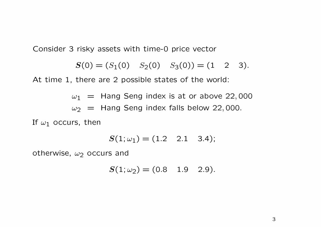
Consider 3 risky assets with time-0 price vector

S(0) = (S1(0) S2(0) S3(0)) = (1 2 3).

At time 1, there are 2 possible states of the world:

ω1 = Hang Seng index is at or above 22,000

ω2 = Hang Seng index falls below 22,000.

If ω1 occurs, then

S(1;ω1) = (1.2 2.1 3.4);

otherwise, ω2 occurs and

S(1;ω2) = (0.8 1.9 2.9).

3

• The possible values of the asset price process at t = 1 are listed

in the following K ×M matrix

S(1; Ω) =

S1(1;ω1) S2(1;ω1) · · · SM(1;ω1)S1(1;ω2) S2(1;ω2) · · · SM(1;ω2)· · · · · · · · · · · ·

S1(1;ωK) S2(1;ωK) · · · SM(1;ωK)

.• Since the assets are limited liability securities, the entries in

S(1; Ω) are non-negative scalars.

• Existence of a strictly positive riskless security or bank account,

whose value is denoted by S0. Without loss of generality, we

take S0(0) = 1 and the value at time 1 to be S0(1) = 1 + r,

where r ≥ 0 is the deterministic interest rate over one period.

4

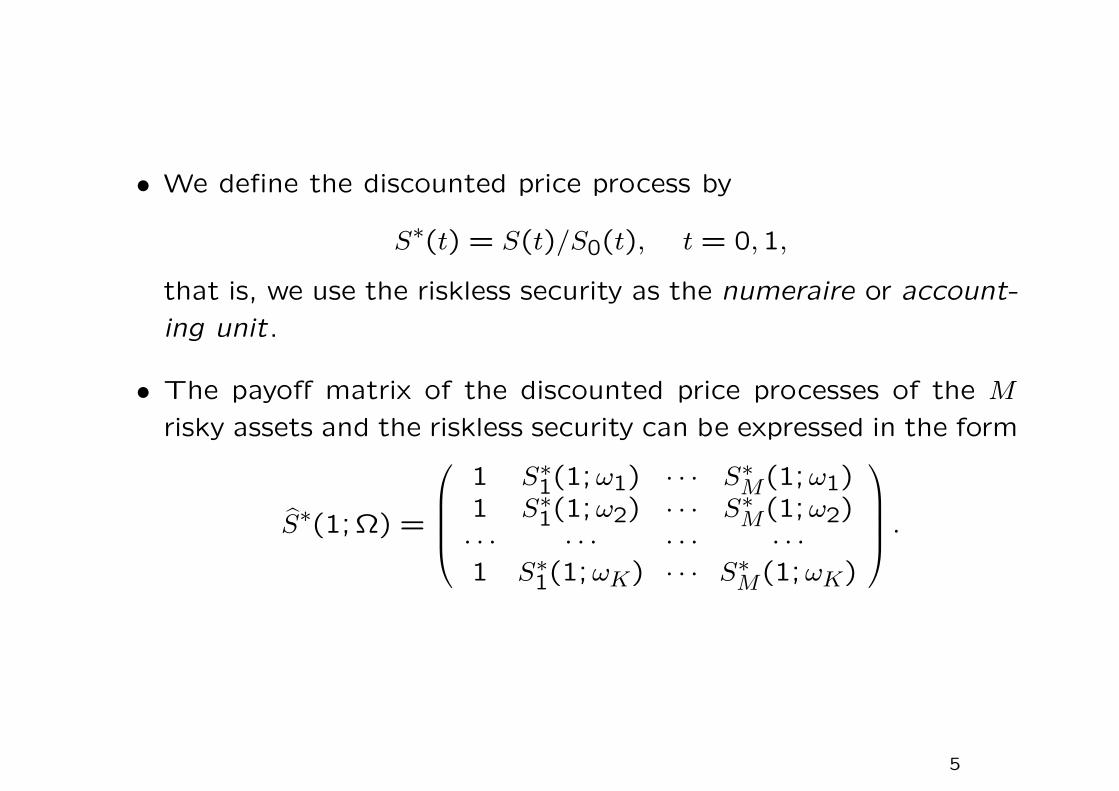
• We define the discounted price process by

S∗(t) = S(t)/S0(t), t = 0,1,

that is, we use the riskless security as the numeraire or account-

ing unit.

• The payoff matrix of the discounted price processes of the M

risky assets and the riskless security can be expressed in the form

S∗(1; Ω) =

1 S∗1(1;ω1) · · · S∗M(1;ω1)1 S∗1(1;ω2) · · · S∗M(1;ω2)· · · · · · · · · · · ·1 S∗1(1;ωK) · · · S∗M(1;ωK)

.

5

Trading strategies

• An investor adopts a trading strategy by selecting a portfolio of

the M assets at time 0. A trading strategy is characterized by

asset holding in the portfolio.

• The number of units of asset m held in the portfolio from t = 0

to t = 1 is denoted by hm,m = 0,1, · · · ,M .

• The scalars hm can be positive (long holding), negative (short

selling) or zero (no holding).

• An investor is endowed with an initial endowment V0 at time 0

to set up the trading portfolio. How do we choose the portfolio

holding of the assets such that the expected portfolio value at

time 1 is maximized?

6

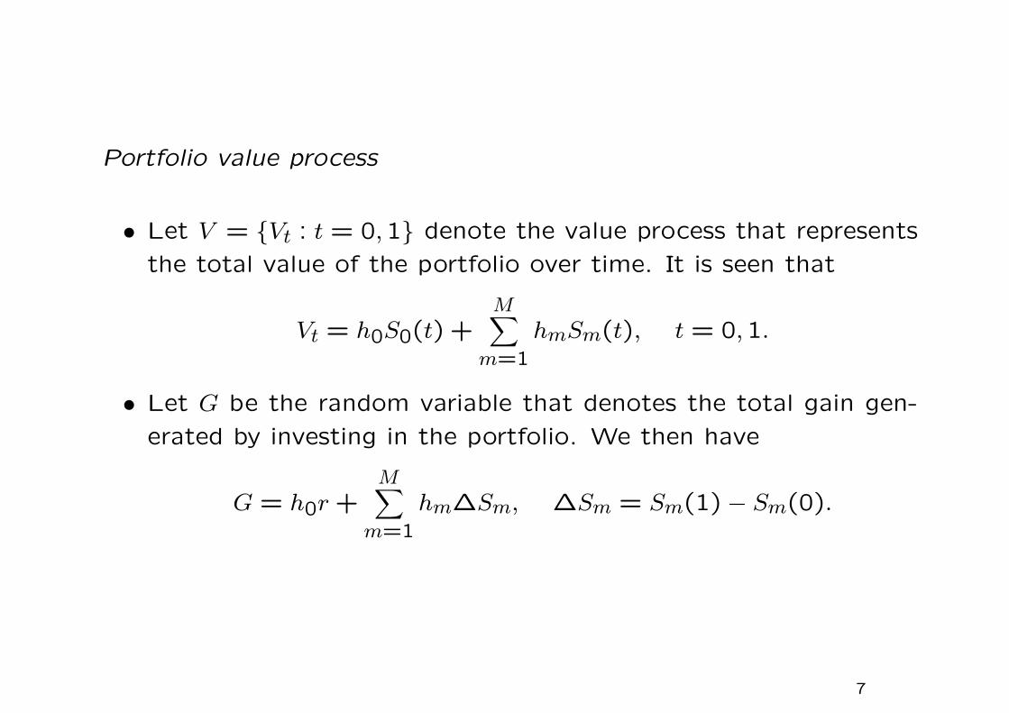
Portfolio value process

• Let V = Vt : t = 0,1 denote the value process that represents

the total value of the portfolio over time. It is seen that

Vt = h0S0(t) +M∑

m=1

hmSm(t), t = 0,1.

• Let G be the random variable that denotes the total gain gen-

erated by investing in the portfolio. We then have

G = h0r +M∑

m=1

hm∆Sm, ∆Sm = Sm(1)− Sm(0).

7

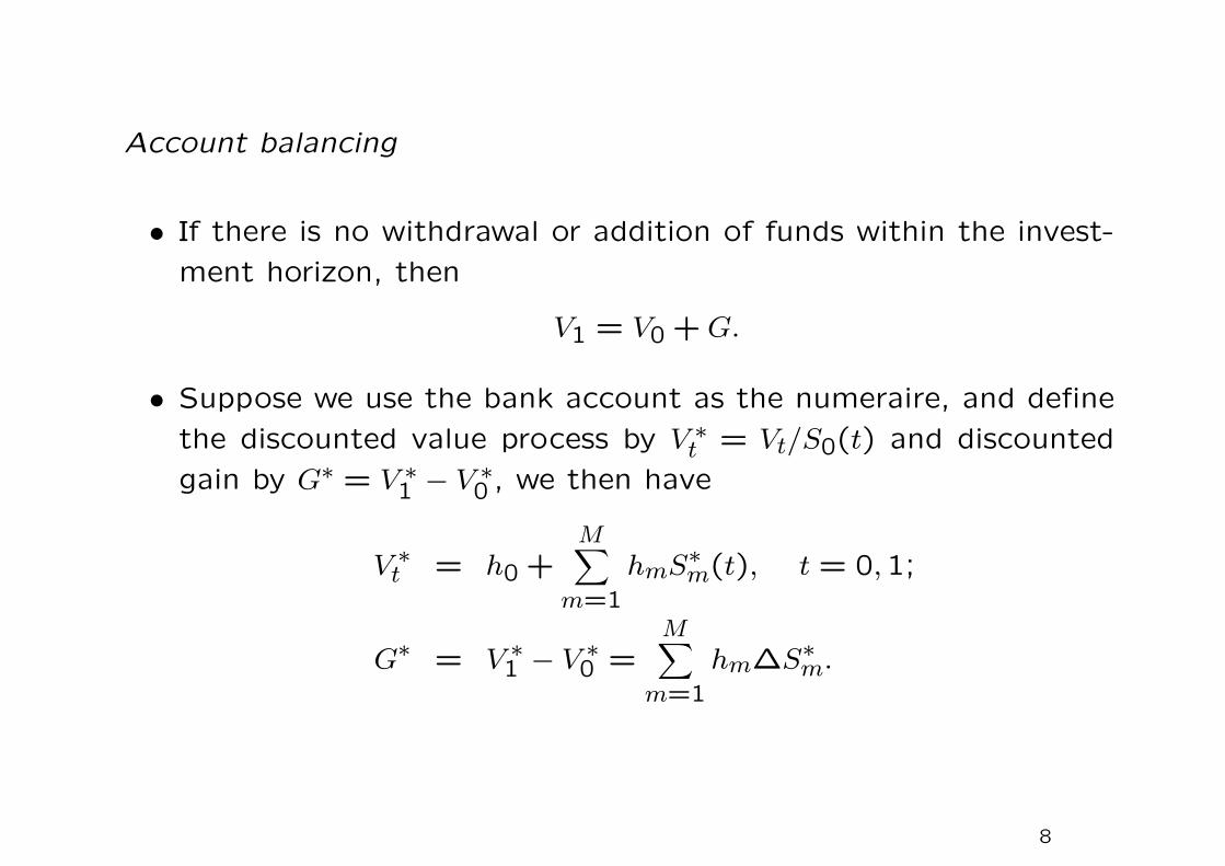
Account balancing

• If there is no withdrawal or addition of funds within the invest-

ment horizon, then

V1 = V0 +G.

• Suppose we use the bank account as the numeraire, and define

the discounted value process by V ∗t = Vt/S0(t) and discounted

gain by G∗ = V ∗1 − V∗

0 , we then have

V ∗t = h0 +M∑

m=1

hmS∗m(t), t = 0,1;

G∗ = V ∗1 − V∗

0 =M∑

m=1

hm∆S∗m.

8

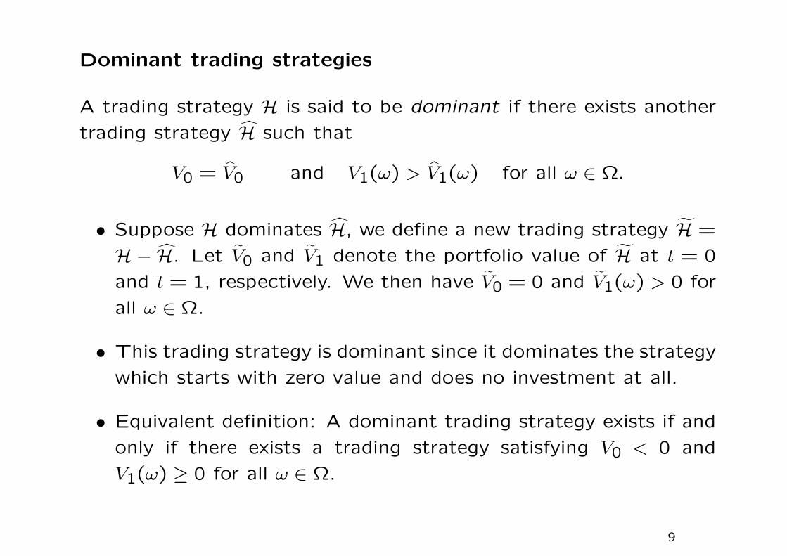
Dominant trading strategies

A trading strategy H is said to be dominant if there exists another

trading strategy H such that

V0 = V0 and V1(ω) > V1(ω) for all ω ∈ Ω.

• Suppose H dominates H, we define a new trading strategy H =

H− H. Let V0 and V1 denote the portfolio value of H at t = 0

and t = 1, respectively. We then have V0 = 0 and V1(ω) > 0 for

all ω ∈ Ω.

• This trading strategy is dominant since it dominates the strategy

which starts with zero value and does no investment at all.

• Equivalent definition: A dominant trading strategy exists if and

only if there exists a trading strategy satisfying V0 < 0 and

V1(ω) ≥ 0 for all ω ∈ Ω.

9

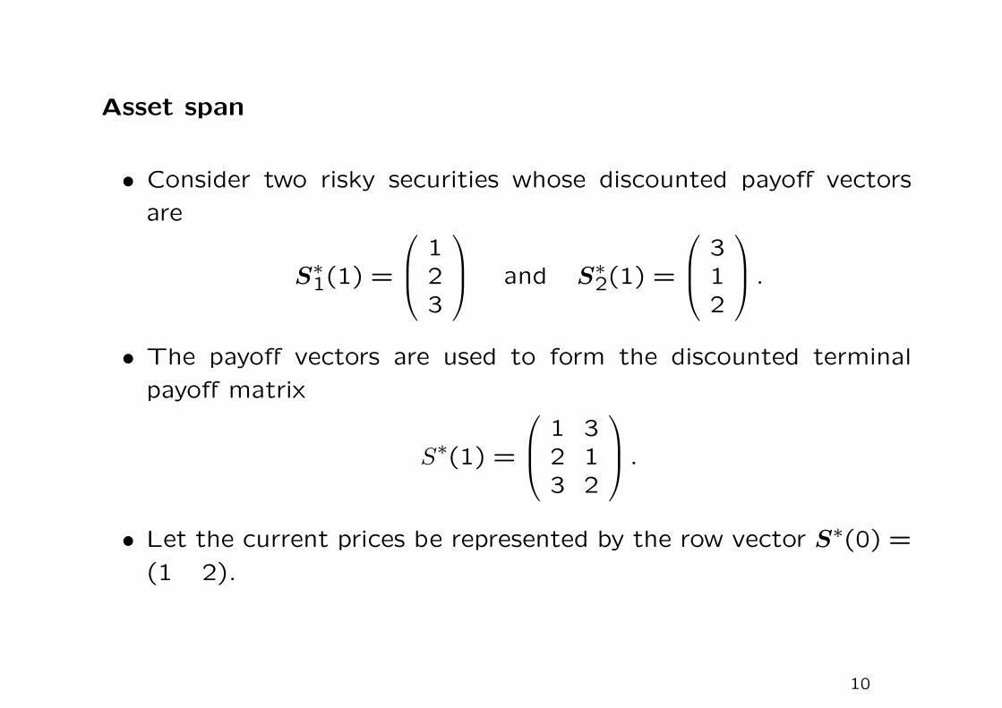
Asset span

• Consider two risky securities whose discounted payoff vectors

are

S∗1(1) =

123

and S∗2(1) =

312

.• The payoff vectors are used to form the discounted terminal

payoff matrix

S∗(1) =

1 32 13 2

.• Let the current prices be represented by the row vector S∗(0) =

(1 2).

10

• We write h as the column vector whose entries are the portfolio

holding of the securities in the portfolio. The trading strategy is

characterized by specifying h. The current portfolio value and

the discounted portfolio payoff are given by S∗(0)h and S∗(1)h,

respectively.

• The set of all portfolio payoffs via different holding of securities

is called the asset span S. The asset span is seen to be the

column space of the payoff matrix S∗(1), which is a subspace in

RK spanned by the columns of S∗(1).

11

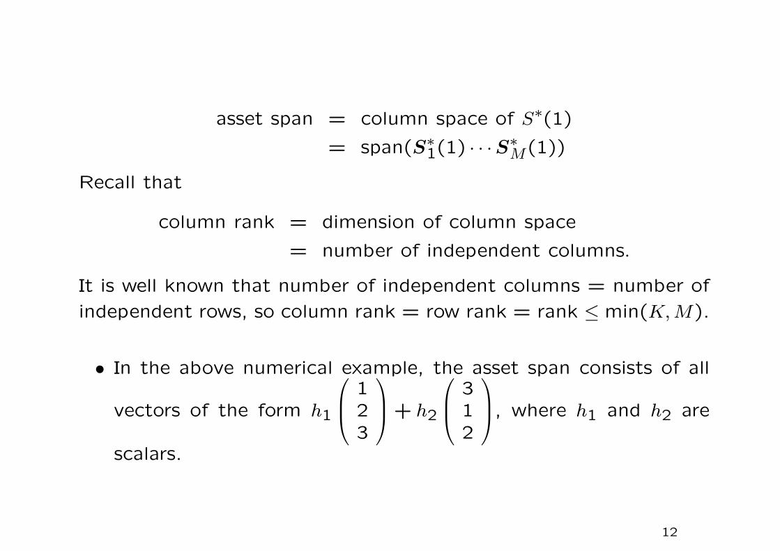
asset span = column space of S∗(1)

= span(S∗1(1) · · ·S∗M(1))

Recall that

column rank = dimension of column space

= number of independent columns.

It is well known that number of independent columns = number of

independent rows, so column rank = row rank = rank ≤ min(K,M).

• In the above numerical example, the asset span consists of all

vectors of the form h1

123

+ h2

312

, where h1 and h2 are

scalars.

12

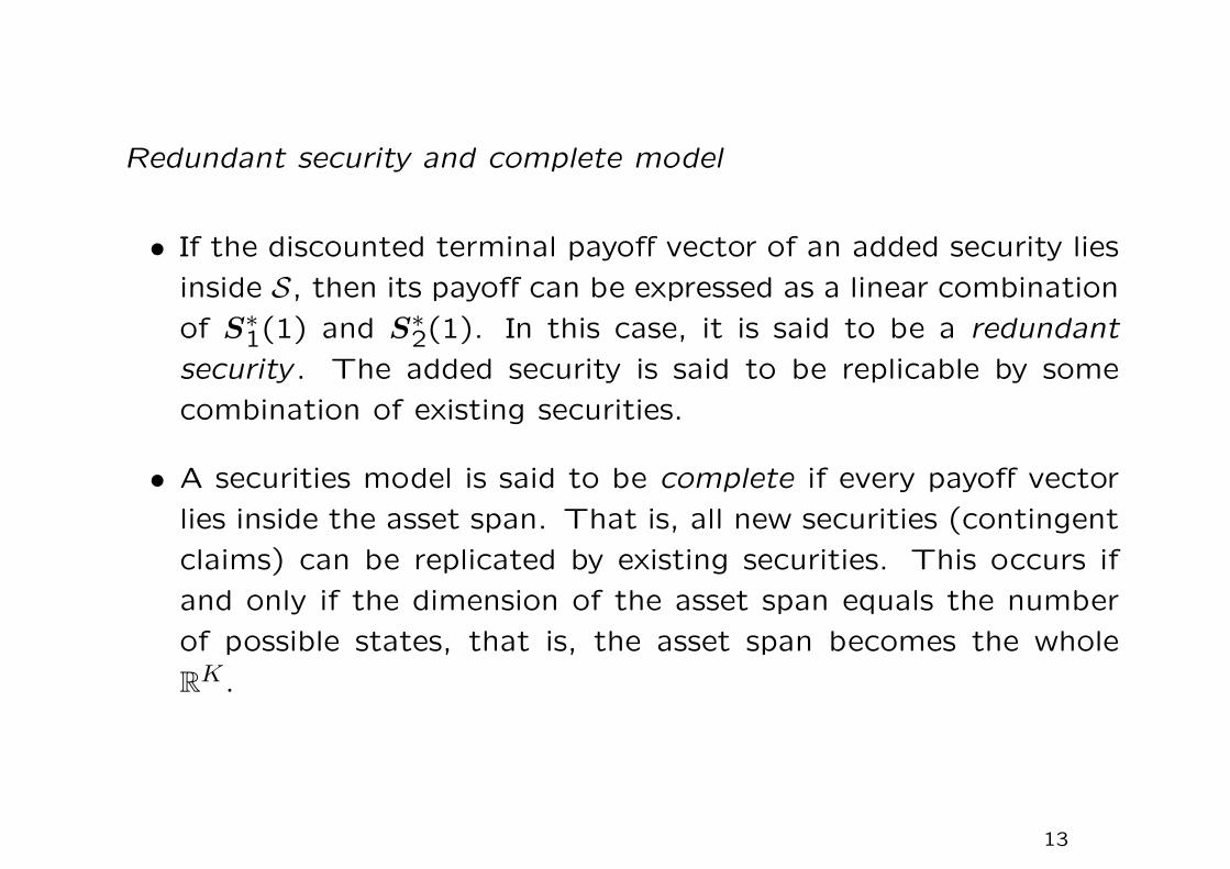
Redundant security and complete model

• If the discounted terminal payoff vector of an added security lies

inside S, then its payoff can be expressed as a linear combination

of S∗1(1) and S∗2(1). In this case, it is said to be a redundant

security . The added security is said to be replicable by some

combination of existing securities.

• A securities model is said to be complete if every payoff vector

lies inside the asset span. That is, all new securities (contingent

claims) can be replicated by existing securities. This occurs if

and only if the dimension of the asset span equals the number

of possible states, that is, the asset span becomes the whole

RK.

13

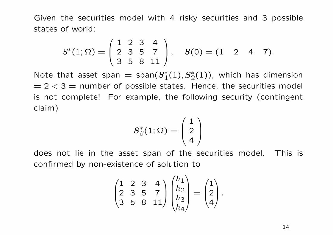
Given the securities model with 4 risky securities and 3 possible

states of world:

S∗(1; Ω) =

1 2 3 42 3 5 73 5 8 11

, S(0) = (1 2 4 7).

Note that asset span = span(S∗1(1),S∗2(1)), which has dimension

= 2 < 3 = number of possible states. Hence, the securities model

is not complete! For example, the following security (contingent

claim)

S∗β(1; Ω) =

124

does not lie in the asset span of the securities model. This is

confirmed by non-existence of solution to1 2 3 42 3 5 73 5 8 11

h1h2h3h4

=

124

.

14

Pricing problem

Given a contingent claim that is replicable by existing securities, its

price with reference to a given securities model is given by the cost

of setting up the replicating portfolio.

Consider a new security with discounted payoff at t = 1 as given by

S∗α(1; Ω) =

58

13

,which is seen to be

S∗α(1; Ω) = S∗2(1; Ω) + S∗3(1; Ω) = S∗1(1; Ω) + 2S∗2(1; Ω).

This new security is redundant. Unfortunately, the price of this

security can be either

S2(0) + S3(0) = 6 or S1(0) + 2S2(0) = 5.

There are two possible prices, corresponding to two different choices

of the replicating portfolio.

15

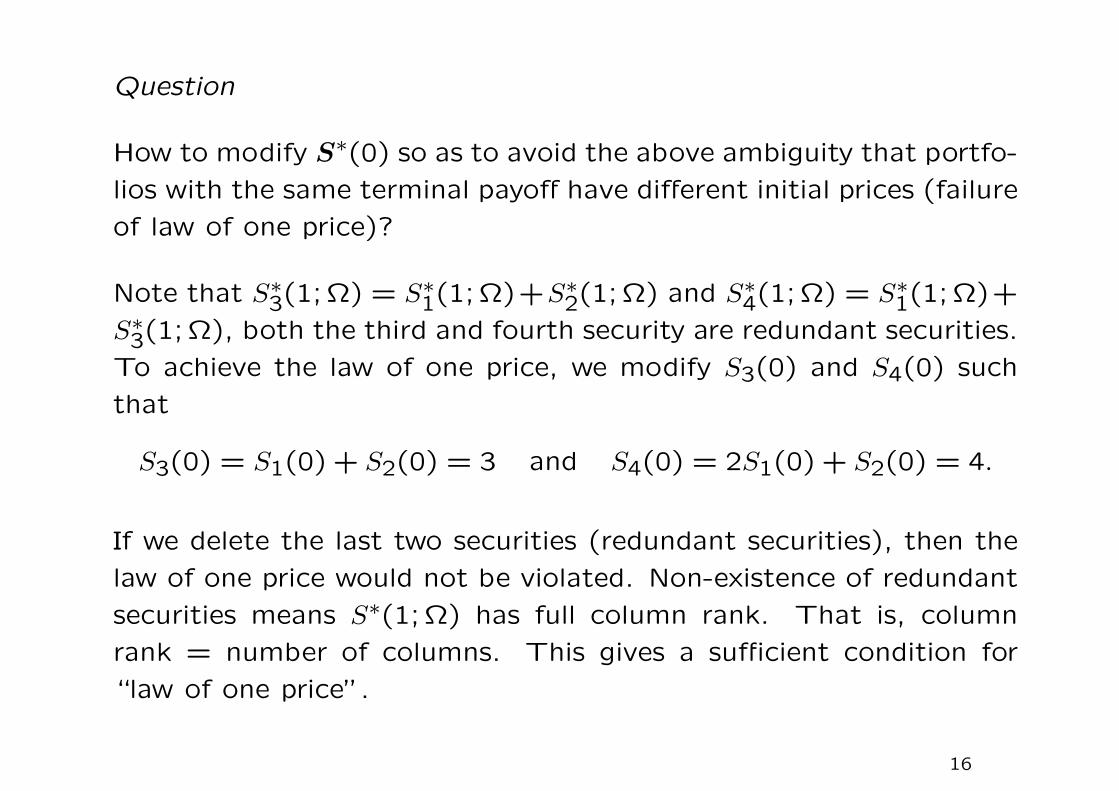
Question

How to modify S∗(0) so as to avoid the above ambiguity that portfo-

lios with the same terminal payoff have different initial prices (failure

of law of one price)?

Note that S∗3(1; Ω) = S∗1(1; Ω)+S∗2(1; Ω) and S∗4(1; Ω) = S∗1(1; Ω)+

S∗3(1; Ω), both the third and fourth security are redundant securities.

To achieve the law of one price, we modify S3(0) and S4(0) such

that

S3(0) = S1(0) + S2(0) = 3 and S4(0) = 2S1(0) + S2(0) = 4.

If we delete the last two securities (redundant securities), then the

law of one price would not be violated. Non-existence of redundant

securities means S∗(1; Ω) has full column rank. That is, column

rank = number of columns. This gives a sufficient condition for

“law of one price”.

16

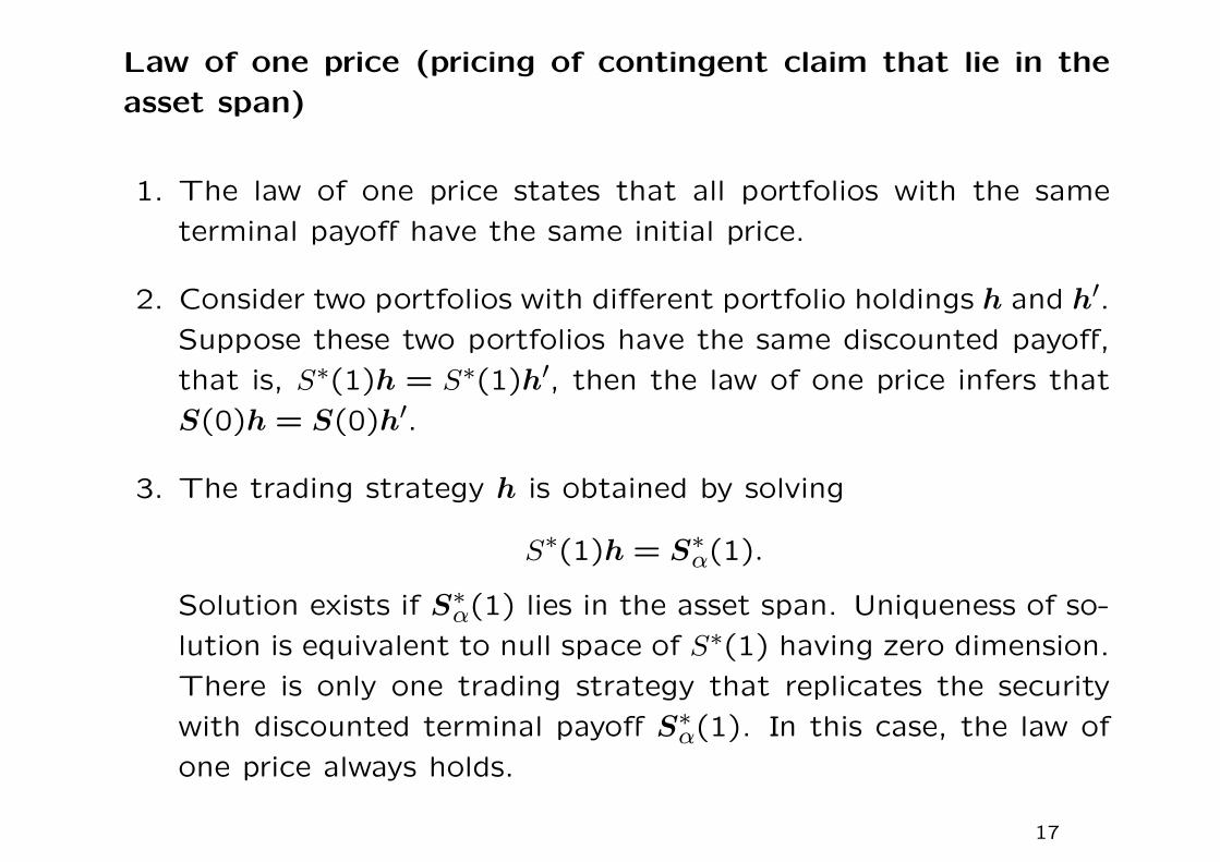
Law of one price (pricing of contingent claim that lie in the

asset span)

1. The law of one price states that all portfolios with the same

terminal payoff have the same initial price.

2. Consider two portfolios with different portfolio holdings h and h′.Suppose these two portfolios have the same discounted payoff,

that is, S∗(1)h = S∗(1)h′, then the law of one price infers that

S(0)h = S(0)h′.

3. The trading strategy h is obtained by solving

S∗(1)h = S∗α(1).

Solution exists if S∗α(1) lies in the asset span. Uniqueness of so-

lution is equivalent to null space of S∗(1) having zero dimension.

There is only one trading strategy that replicates the security

with discounted terminal payoff S∗α(1). In this case, the law of

one price always holds.

17

Law of one price and dominant trading strategy

If the law of one price fails, then it is possible to have two trading

strategies h and h′ such that S∗(1)h = S∗(1)h′ but S(0)h > S(0)h′.

Let G∗(ω) and G∗′(ω) denote the respective discounted gain corre-

sponding to the trading strategies h and h′. We then have G∗′(ω) >

G∗(ω) for all ω ∈ Ω, so there exists a dominant trading strategy. The

corresponding dominant trading strategy is h′ − h so that V0 < 0

but V ∗1 (ω) = 0 for all ω ∈ Ω.

Hence, the non-existence of dominant trading strategy implies the

law of one price. However, the converse statement does not hold.

[See a later numerical example on p.36]

18

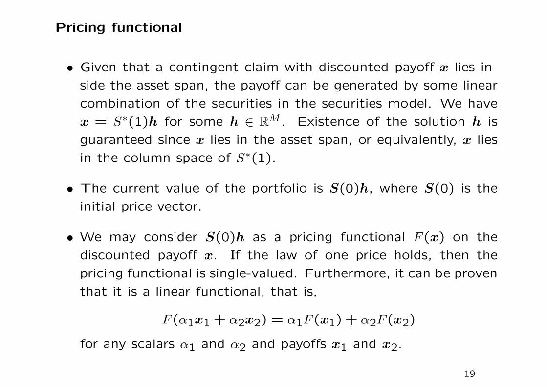
Pricing functional

• Given that a contingent claim with discounted payoff x lies in-

side the asset span, the payoff can be generated by some linear

combination of the securities in the securities model. We have

x = S∗(1)h for some h ∈ RM . Existence of the solution h is

guaranteed since x lies in the asset span, or equivalently, x lies

in the column space of S∗(1).

• The current value of the portfolio is S(0)h, where S(0) is the

initial price vector.

• We may consider S(0)h as a pricing functional F (x) on the

discounted payoff x. If the law of one price holds, then the

pricing functional is single-valued. Furthermore, it can be proven

that it is a linear functional, that is,

F (α1x1 + α2x2) = α1F (x1) + α2F (x2)

for any scalars α1 and α2 and payoffs x1 and x2.

19

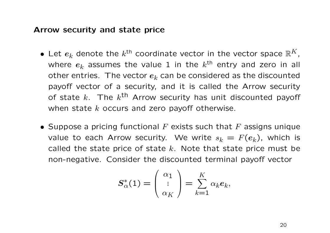
Arrow security and state price

• Let ek denote the kth coordinate vector in the vector space RK,

where ek assumes the value 1 in the kth entry and zero in all

other entries. The vector ek can be considered as the discounted

payoff vector of a security, and it is called the Arrow security

of state k. The kth Arrow security has unit discounted payoff

when state k occurs and zero payoff otherwise.

• Suppose a pricing functional F exists such that F assigns unique

value to each Arrow security. We write sk = F (ek), which is

called the state price of state k. Note that state price must be

non-negative. Consider the discounted terminal payoff vector

S∗α(1) =

α1...αK

=K∑k=1

αkek,

20

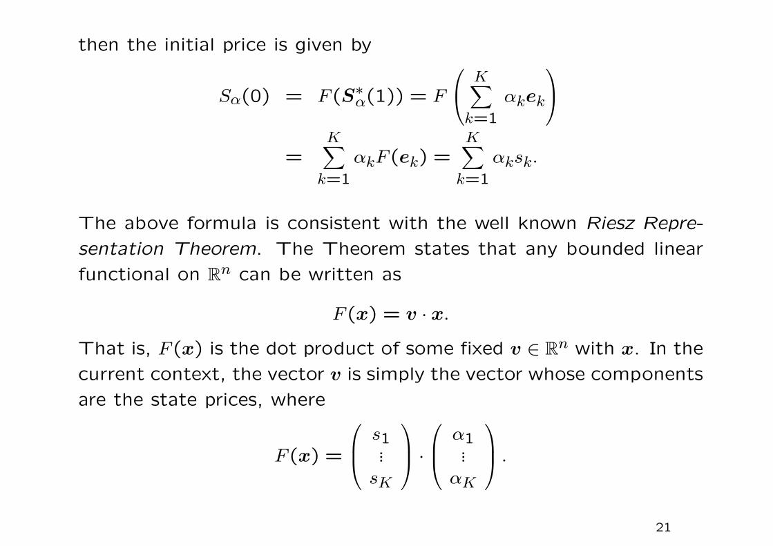
then the initial price is given by

Sα(0) = F (S∗α(1)) = F

K∑k=1

αkek

=

K∑k=1

αkF (ek) =K∑k=1

αksk.

The above formula is consistent with the well known Riesz Repre-

sentation Theorem. The Theorem states that any bounded linear

functional on Rn can be written as

F (x) = v · x.

That is, F (x) is the dot product of some fixed v ∈ Rn with x. In the

current context, the vector v is simply the vector whose components

are the state prices, where

F (x) =

s1...sK

· α1

...αK

.21

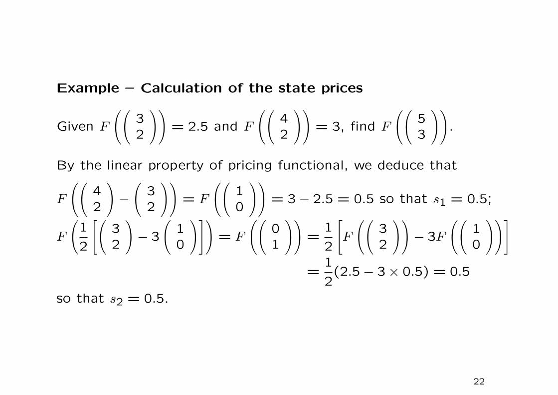
Example – Calculation of the state prices

Given F

((32

))= 2.5 and F

((42

))= 3, find F

((53

)).

By the linear property of pricing functional, we deduce that

F

((42

)−(

32

))= F

((10

))= 3− 2.5 = 0.5 so that s1 = 0.5;

F

(1

2

[(32

)− 3

(10

)])= F

((01

))=

1

2

[F

((32

))− 3F

((10

))]

=1

2(2.5− 3× 0.5) = 0.5

so that s2 = 0.5.

22

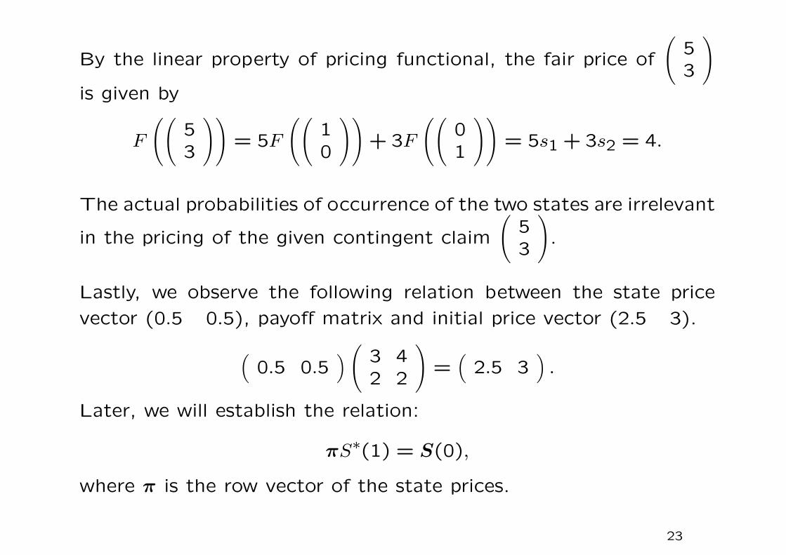
By the linear property of pricing functional, the fair price of

(53

)is given by

F

((53

))= 5F

((10

))+ 3F

((01

))= 5s1 + 3s2 = 4.

The actual probabilities of occurrence of the two states are irrelevant

in the pricing of the given contingent claim

(53

).

Lastly, we observe the following relation between the state price

vector (0.5 0.5), payoff matrix and initial price vector (2.5 3).

(0.5 0.5

)( 3 42 2

)=(

2.5 3).

Later, we will establish the relation:

πS∗(1) = S(0),

where π is the row vector of the state prices.

23

Summary

Given a securities model endowed with S∗(1; Ω) and S(0), can we

find a trading strategy to form a portfolio that replicates a new

security with discounted terminal payoff vector S∗α(1; Ω) (also called

a contingent claim) that is outside the universe of the M available

risky securities in the securities model?

Replication means the terminal payoff of the replicating portfolio

matches with that of the contingent claim under all scenarios of

occurrence of the state of the world at t = 1.

1. Formation of the replicating portfolio is possible if we have ex-

istence of solution h to the following system

S∗(1; Ω)h = S∗α(1; Ω).

This is equivalent to the fact that “S∗α(1; Ω) lies in the asset

span (column space) of S∗(1; Ω)”. The solution h is the corre-

sponding trading strategy. Note that h may not be unique.

24

Completeness of securities model

If all contingent claims are replicable, then the securities model is

said to be complete. This is equivalent to

dim(asset span) = K = number of possible states,

that is, asset span = RK. In this case, solution h always exists.

Relation between null space and row space of matrix A

Given a matrix A, the null space of η(A) is given by

η(A) = x : Ax = 0.

Every vector in η(A) is orthogonal to every row in A. If we define

the orthogonal complement of η(A) by

η(A)⊥ = y : y · x = 0 for all x ∈ η(A),

then η(A)⊥ is seen to be the row space of A. Pick any vector x

in the null space and any vector y in the row space, they must be

orthogonal to each other.

25

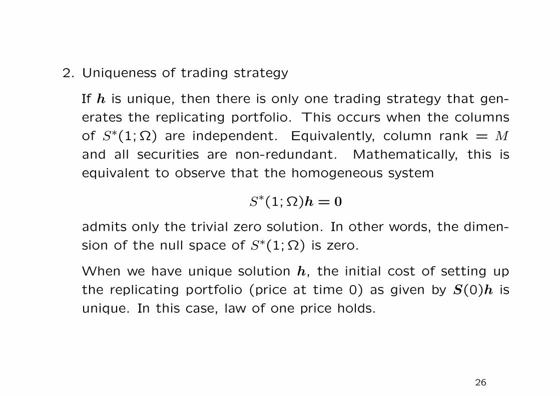
2. Uniqueness of trading strategy

If h is unique, then there is only one trading strategy that gen-

erates the replicating portfolio. This occurs when the columns

of S∗(1; Ω) are independent. Equivalently, column rank = M

and all securities are non-redundant. Mathematically, this is

equivalent to observe that the homogeneous system

S∗(1; Ω)h = 0

admits only the trivial zero solution. In other words, the dimen-

sion of the null space of S∗(1; Ω) is zero.

When we have unique solution h, the initial cost of setting up

the replicating portfolio (price at time 0) as given by S(0)h is

unique. In this case, law of one price holds.

26

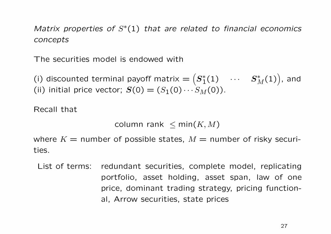
Matrix properties of S∗(1) that are related to financial economics

concepts

The securities model is endowed with

(i) discounted terminal payoff matrix =(S∗1(1) · · · S∗M(1)

), and

(ii) initial price vector; S(0) = (S1(0) · · ·SM(0)).

Recall that

column rank ≤ min(K,M)

where K = number of possible states, M = number of risky securi-

ties.

List of terms: redundant securities, complete model, replicating

portfolio, asset holding, asset span, law of one

price, dominant trading strategy, pricing function-

al, Arrow securities, state prices

27

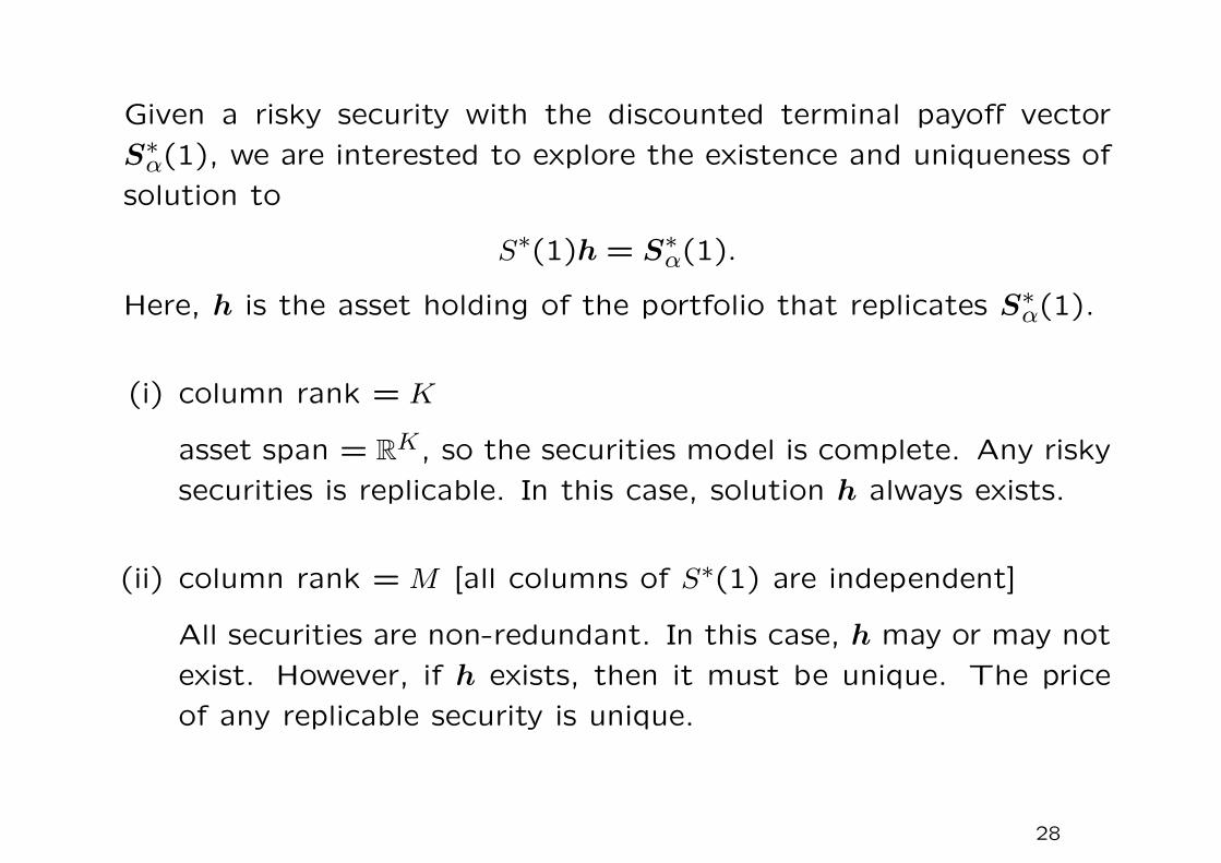
Given a risky security with the discounted terminal payoff vector

S∗α(1), we are interested to explore the existence and uniqueness of

solution to

S∗(1)h = S∗α(1).

Here, h is the asset holding of the portfolio that replicates S∗α(1).

(i) column rank = K

asset span = RK, so the securities model is complete. Any risky

securities is replicable. In this case, solution h always exists.

(ii) column rank = M [all columns of S∗(1) are independent]

All securities are non-redundant. In this case, h may or may not

exist. However, if h exists, then it must be unique. The price

of any replicable security is unique.

28

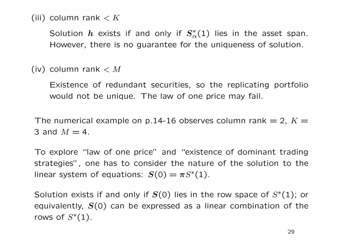
(iii) column rank < K

Solution h exists if and only if S∗α(1) lies in the asset span.

However, there is no guarantee for the uniqueness of solution.

(iv) column rank < M

Existence of redundant securities, so the replicating portfolio

would not be unique. The law of one price may fail.

The numerical example on p.14-16 observes column rank = 2, K =

3 and M = 4.

To explore “law of one price” and “existence of dominant trading

strategies”, one has to consider the nature of the solution to the

linear system of equations: S(0) = πS∗(1).

Solution exists if and only if S(0) lies in the row space of S∗(1); or

equivalently, S(0) can be expressed as a linear combination of the

rows of S∗(1).

29

Law of one price revisited

Law of one price holds if and only if solution to

πS∗(1) = S(0) (A)

exists.

1. Suppose solution to (A) exists, let h and h′ be two trading

strategies such that their respective discounted terminal payoff

V and V ′ are the same. That is,

S∗(1)h = V = V ′ = S∗(1)h′.

Since π exists, we multiply both sides by π and obtain

πS∗(1)(h− h′) = 0.

Noting that πS∗(1) = S(0), we obtain

S(0)(h− h′) = 0 so that V0 = V ′0.

Hence, law of one price is established.

30

2. Suppose solution to (A) does not exist for the given S(0), this

implies that S(0) that does not lie in the row space of S∗(1).

The row space of S∗(1) does not span the whole RM . There-

fore, dim(row space of S∗(1)) < M , where M is the number of

securities = number of columns in S∗(1).

Recall that

dim(null space of S∗(1)) + rank(S∗(1)) = M

so that dim(null space of S∗(1)) > 0.

Hence, there exists non-zero solution h to

S∗(1)h = 0.

Note that h is orthogonal to all rows of S∗(1), and recall that

row space = orthogonal complement of null space.

31

Also, there always exists a non-zero solution h that is not orthogonal

to S(0). If otherwise, S(0) is orthogonal to every vector in the null

space, so it lies in the orthogonal complement of the null space

(that is, row space). This leads to a contradiction since S(0) does

not lie in the row space.

Consider the above choice of h that lies in the null space, where

S(0)h 6= 0; we let h = h1 − h2, where h1 6= h2. Since S∗(1)(h1 −h2) = 0, then there exist two distinct trading strategies such that

S∗(1)h1 = S∗(1)h2.

The two strategies have the same discounted terminal payoff under

all states of the world. However, their initial prices are unequal since

S(0)h1 6= S(0)h2,

by virtue of the property: S(0)h 6= 0. Hence, the law of one price

does not hold.

32

Linear pricing measure

We consider securities models with the inclusion of the riskfree se-

curity. A non-negative row vector q = (q(ω1) · · · q(ωK)) is said to be

a linear pricing measure if for every trading strategy the portfolio

values at t = 0 and t = 1 are related by

V0 =K∑k=1

q(ωk)V ∗1 (ωk).

Note that q is not required to be unique.

Remark

Here, the same initial price V0 is always resulted as there is no de-

pendence of V0 on the asset holding of the portfolio. Two portfolios

with different holdings of securities but the same terminal payoff for

all states of the world would have the same price. Implicitly, this

implies that the law of one price holds. The rigorous justification

of the above statement will be presented later.

33

1. Suppose we take the holding amount of every risky security to

be zero, thereby h1 = h2 = · · · = hM = 0, leaving only the

riskfree security. This gives

V0 = h0 =K∑k=1

q(ωk)h0

so thatK∑k=1

q(ωk) = 1.

• Since we have taken q(ωk) ≥ 0, k = 1, · · · ,K, and their sum is

one, we may interpret q(ωk) as a probability measure on the

sample space Ω.

• Note that q(ωk) is not related to the actual probability of occur-

rence of the state k, though the current security price is given

by the expectation of the discounted security payoff one period

later under the linear pricing measure.

34

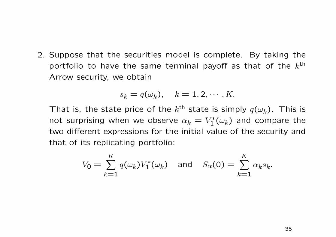
2. Suppose that the securities model is complete. By taking the

portfolio to have the same terminal payoff as that of the kth

Arrow security, we obtain

sk = q(ωk), k = 1,2, · · · ,K.

That is, the state price of the kth state is simply q(ωk). This is

not surprising when we observe αk = V ∗1 (ωk) and compare the

two different expressions for the initial value of the security and

that of its replicating portfolio:

V0 =K∑k=1

q(ωk)V ∗1 (ωk) and Sα(0) =K∑k=1

αksk.

35

• By taking the portfolio weights to be zero except for the mth

security, we have

Sm(0) =K∑k=1

q(ωk)S∗m(1;ωk), m = 0,1, · · · ,M.

Putting these m+1 components into the matrix form, we obtain

S(0) = qS∗(1; Ω), q ≥ 0.

The system of algebraic equations resembles that in law of one

price discussion except that we require (i) nonnegative solution

q ≥ 0, (ii) inclusion of the riskfree asset.

We may rewrite the M + 1 equations as

K∑k=1

q(wk)∆S∗m(1;ωk) = 0, m = 0,1, . . . ,M.

36

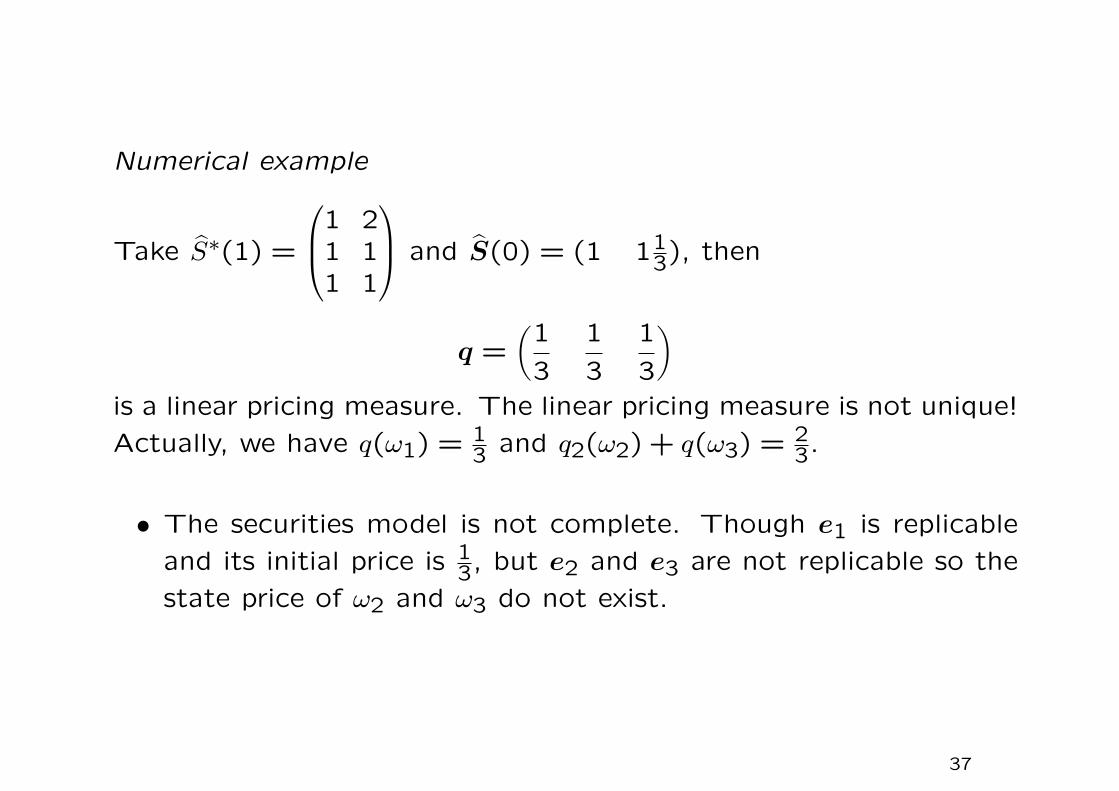
Numerical example

Take S∗(1) =

1 21 11 1

and S(0) = (1 113), then

q =(

1

3

1

3

1

3

)is a linear pricing measure. The linear pricing measure is not unique!

Actually, we have q(ω1) = 13 and q2(ω2) + q(ω3) = 2

3.

• The securities model is not complete. Though e1 is replicable

and its initial price is 13, but e2 and e3 are not replicable so the

state price of ω2 and ω3 do not exist.

37

Suppose we add the new risky security with discounted terminal

payoff

121

and initial price 23 into the securities model, then the

securities model becomes complete. It is unreasonable to set the

initial price of

121

to be below that of

111

. This leads to negative

state price of the second Arrow security. Indeed, we obtain the

following state prices

s1 =1

3, s2 = −

1

3s3 = 1.

In this case, law of one price holds but dominant trading strategy

exists. For example, we may take

V ∗1 (ω) =

361

> 0, V0 = 3s1 + 6s2 + s3 = 0.

38

Example – Law of one price

Take S∗(1; Ω) =

1 2 6 91 3 3 71 6 12 19

, the sum of the first 3 columns

gives the fourth column. The first column corresponds to the dis-

counted terminal payoff of the riskfree security under the 3 possible

states of the world. The third risky security is a redundant security.

Let S(0) = (1 2 3 k). We observe that solution to

(1 2 3 k) = (π1 π2 π3)

1 2 6 91 3 3 71 6 12 19

(A)

exists if and only if k = 6. That is, S3(0) = S0(0) + S1(0) + S2(0).

When k 6= 6, the law of one price does not hold. The last equation:

9π1 + 7π2 + 19π3 = k 6= 6 is inconsistent with the first 3 equations.

One may check that (1 2 3 6) can be expressed as a linear

combination of the rows of S∗(1; Ω).

39

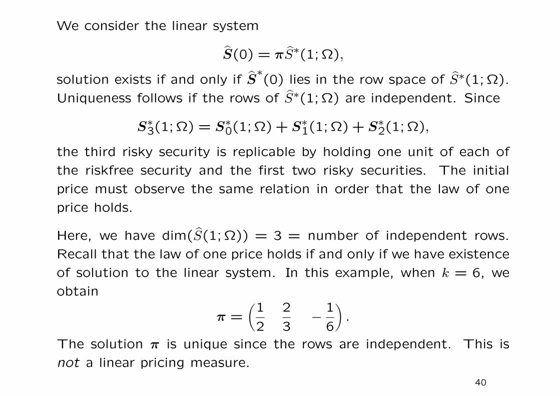
We consider the linear system

S(0) = πS∗(1; Ω),

solution exists if and only if S∗(0) lies in the row space of S∗(1; Ω).

Uniqueness follows if the rows of S∗(1; Ω) are independent. Since

S∗3(1; Ω) = S∗0(1; Ω) + S∗1(1; Ω) + S∗2(1; Ω),

the third risky security is replicable by holding one unit of each of

the riskfree security and the first two risky securities. The initial

price must observe the same relation in order that the law of one

price holds.

Here, we have dim(S(1; Ω)) = 3 = number of independent rows.

Recall that the law of one price holds if and only if we have existence

of solution to the linear system. In this example, when k = 6, we

obtain

π =(

1

2

2

3−

1

6

).

The solution π is unique since the rows are independent. This is

not a linear pricing measure.

40

Example – Law of one price holds while dominant trading

strategies exist

Consider a securities model with 2 risky securities and the riskfree

security, and there are 3 possible states. The current discounted

price vector S(0) is (1 4 2) and the discounted payoff matrix at

t = 1 is S∗(1) =

1 4 31 3 21 2 4

.

Here, the law of one price holds since the only solution to S∗(1)h = 0

is h = 0. This is because the columns of S∗(1) are independent so

that the dimension of the nullspace of S∗(1) is zero.

41

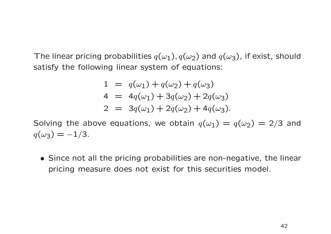
The linear pricing probabilities q(ω1), q(ω2) and q(ω3), if exist, should

satisfy the following linear system of equations:

1 = q(ω1) + q(ω2) + q(ω3)

4 = 4q(ω1) + 3q(ω2) + 2q(ω3)

2 = 3q(ω1) + 2q(ω2) + 4q(ω3).

Solving the above equations, we obtain q(ω1) = q(ω2) = 2/3 and

q(ω3) = −1/3.

• Since not all the pricing probabilities are non-negative, the linear

pricing measure does not exist for this securities model.

42

Theorem

There exists a linear pricing measure if and only if there are no

dominant trading strategies.

The above linear pricing measure theorem can be seen to be a direct

consequence of the Farkas Lemma.

Farkas Lemma

There does not exist h ∈ RM such that

S∗(1; Ω)h > 0 and S(0)h = 0

if and only if there exists q ∈ RK such that

S(0) = qS∗(1; Ω) and q ≥ 0.

43

Given that the security lies in the asset span, we can deduce that

law of one price holds by observing either

(i) null space of S∗(1) has zero dimension, or

(ii) existence of a linear pricing measure.

Both (i) and (ii) represent the various forms of sufficient condition

for the law of one price.

Remarks

1. Condition (i) is equivalent to non-existence of redundant secu-

rities.

2. Condition (i) and condition (ii) are not equivalent, nor one im-

plies the other.

44

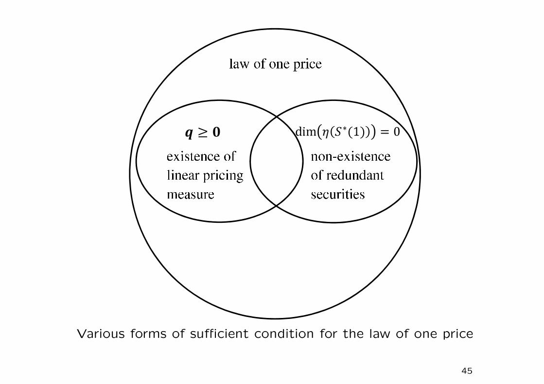
Various forms of sufficient condition for the law of one price

45

2.2 No-arbitrage theory and risk neutral probability measure:

Fundamental Theorem of Asset Pricing

• An arbitrage opportunity is some trading strategy that has the

following properties: (i) V0 = 0, (ii) V ∗1 (ω) ≥ 0 with strict in-

equality at least for one state.

• The existence of a dominant strategy requires a portfolio with

initial zero wealth to end up with a strictly positive wealth in all

states.

• The existence of a dominant trading strategy implies the exis-

tence of an arbitrage opportunity, but the converse is not nec-

essarily true.

46

Risk neutral probability measure

A probability measure Q on Ω is a risk neutral probability measure

if it satisfies

(i) Q(ω) > 0 for all ω ∈ Ω, and

(ii) EQ[∆S∗m] = 0,m = 0,1, · · · ,M , where EQ denotes the expec-

tation under Q. The expectation of the discounted gain of any

security in the securities model under Q is zero.

Note that EQ[∆S∗m] = 0 is equivalent to Sm(0) =K∑k=1

Q(ωk)S∗m(1;ωk).

When m = 0, this leads toK∑k=1

Q(ωk) = 1.

Under absence of arbitrage opportunities, every investor should use

Q(ω) (though not necessarily unique) to find the fair value of an

attainable contingent claim, paying no regard to P (ω).

47

Fundamental Theorem of Asset Pricing

No arbitrage opportunities exist if and only if there exists a risk

neutral probability measure Q.

Proof of Theorem “⇐ part”.

Assume that a risk neutral probability measure Q exists, that is,

S(0) = πS∗(1; Ω), where π = (Q(ω1) · · ·Q(ωK)) and π > 0. We

would like to show that it is never possible to construct a trading

strategy that represents an arbitrage opportunity.

Suppose we claim that an arbitrage opportunity exists where there

exists a trading strategy h = (h0 h1 · · · hM)T ∈ RM+1 such that

S(0)h = 0 and S∗(1; Ω)h ≥ 0 in all ω ∈ Ω and with strict inequality

in at least one state. Now consider S(0)h = πS∗(1; Ω)h, it is seen

that S(0)h > 0 since all entries in π are strictly positive and entries

in S∗(1; Ω)h are either zero or strictly positive (at least for one

state). This leads to a contradiction since it is impossible to have

S(0)h = 0 and S∗(1; Ω)h ≥ 0 in all ω ∈ Ω, with strict inequality in

at least one state.48

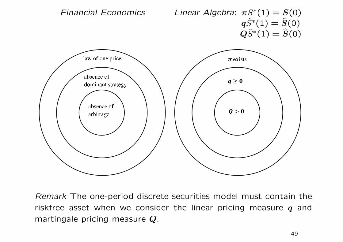
Financial Economics Linear Algebra: πS∗(1) = S(0)qS∗(1) = S(0)QS∗(1) = S(0)

Remark The one-period discrete securities model must contain the

riskfree asset when we consider the linear pricing measure q and

martingale pricing measure Q.

49

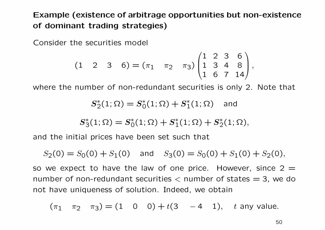
Example (existence of arbitrage opportunities but non-existence

of dominant trading strategies)

Consider the securities model

(1 2 3 6) = (π1 π2 π3)

1 2 3 61 3 4 81 6 7 14

,where the number of non-redundant securities is only 2. Note that

S∗2(1; Ω) = S∗0(1; Ω) + S∗1(1; Ω) and

S∗3(1; Ω) = S∗0(1; Ω) + S∗1(1; Ω) + S∗2(1; Ω),

and the initial prices have been set such that

S2(0) = S0(0) + S1(0) and S3(0) = S0(0) + S1(0) + S2(0),

so we expect to have the law of one price. However, since 2 =

number of non-redundant securities < number of states = 3, we do

not have uniqueness of solution. Indeed, we obtain

(π1 π2 π3) = (1 0 0) + t(3 − 4 1), t any value.

50

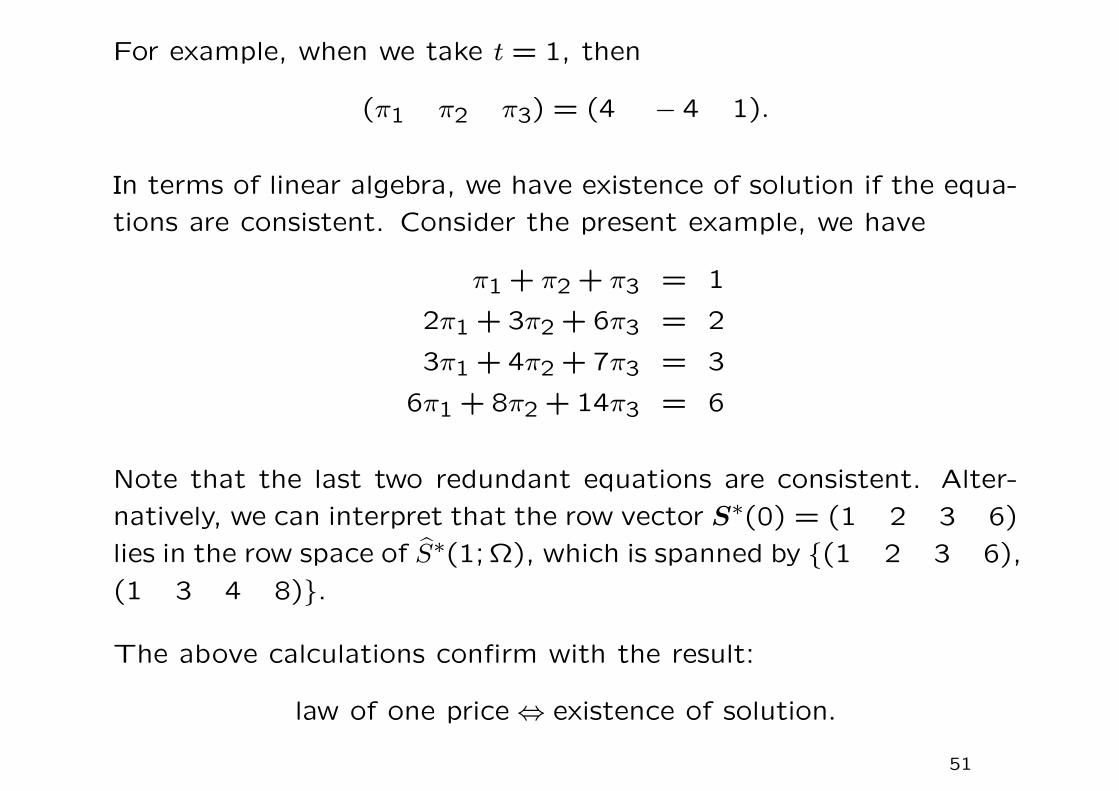
For example, when we take t = 1, then

(π1 π2 π3) = (4 − 4 1).

In terms of linear algebra, we have existence of solution if the equa-

tions are consistent. Consider the present example, we have

π1 + π2 + π3 = 1

2π1 + 3π2 + 6π3 = 2

3π1 + 4π2 + 7π3 = 3

6π1 + 8π2 + 14π3 = 6

Note that the last two redundant equations are consistent. Alter-

natively, we can interpret that the row vector S∗(0) = (1 2 3 6)

lies in the row space of S∗(1; Ω), which is spanned by (1 2 3 6),

(1 3 4 8).

The above calculations confirm with the result:

law of one price⇔ existence of solution.

51

In this securities model, we cannot find a risk neutral measure where

(Q1 Q2 Q3) > 0. This is easily seen since π2 = −4t and π3 = t,

and they always have opposite sign. However, a linear pricing mea-

sure exists. By setting t = 0, we obtain the linear pricing measure

(q1 q2 q3) = (1 0 0) ≥ 0.

Since Q does not exist, the securities model admits arbitrage op-

portunities. One such example is h = (−11 1 1 1)T , where

S(0)h = 0 and S∗(1; Ω)h =

1 2 3 61 3 4 81 6 7 14

−11

111

=

04

16

.

We start with zero portfolio value at t = 0 while the discounted

portfolio value at t = 1 is guaranteed to be non-negative, with

strict positivity for at least one state. This signifies an arbitrage

opportunity.

52

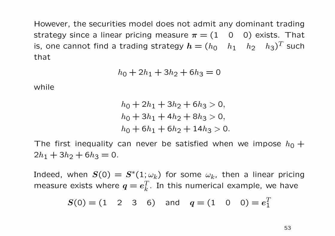
However, the securities model does not admit any dominant trading

strategy since a linear pricing measure π = (1 0 0) exists. That

is, one cannot find a trading strategy h = (h0 h1 h2 h3)T such

that

h0 + 2h1 + 3h2 + 6h3 = 0

while

h0 + 2h1 + 3h2 + 6h3 > 0,

h0 + 3h1 + 4h2 + 8h3 > 0,

h0 + 6h1 + 6h2 + 14h3 > 0.

The first inequality can never be satisfied when we impose h0 +

2h1 + 3h2 + 6h3 = 0.

Indeed, when S(0) = S∗(1;ωk) for some ωk, then a linear pricing

measure exists where q = eTk . In this numerical example, we have

S(0) = (1 2 3 6) and q = (1 0 0) = eT1

53

Martingale property is defined for adapted stochastic processes∗

In the context of one-period model, given the information on the

initial prices and terminal payoff values of the security prices at

t = 0, we have

Sm(0) = EQ[S∗m(1; Ω)] =K∑k=1

S∗m(1;ωk)Q(ωk), m = 1,2, · · · ,M.

The discounted security price process S∗m(t) is said to be a martin-

gale† under Q.

Martingale is associated with the wealth process of a gambler in

a fair game. In a fair game, the expected value of the gambler’s

wealth after any number of plays is always equal to her initial wealth.

∗A stochastic process is adapted to a filtration with respect to a measure. SayS∗m is adapted to F = Ft; t = 0,1, · · · , T, then S∗m(t) is Ft-measurable.

†Martingale property with respect to Q and F:

S∗m(t) = EQ[S∗m(s+ t)|Ft] for all t ≥ 0, s ≥ 0.

54

Equivalent martingale measure

The risk neutral probability measure Q is commonly called the equiv-

alent martingale measure. “Equivalent” refers to the equivalence

between the physical measure P and martingale measure Q [observ-

ing P (ω) > 0⇔ Q(ω) > 0 for all ω ∈ Ω]∗. The linear pricing measure

falls short of this equivalence property since q(ω) can be zero for

some ω.

∗P and Q may not agree on the assignment of probability values to individualevents, but they always agree as to which events are possible or impossible.

55

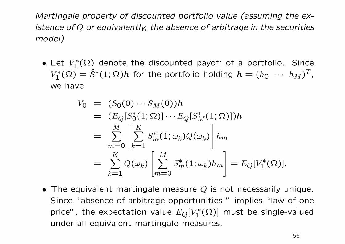
Martingale property of discounted portfolio value (assuming the ex-

istence of Q or equivalently, the absence of arbitrage in the securities

model)

• Let V ∗1 (Ω) denote the discounted payoff of a portfolio. Since

V ∗1 (Ω) = S∗(1; Ω)h for the portfolio holding h = (h0 · · · hM)T ,

we have

V0 = (S0(0) · · ·SM(0))h

= (EQ[S∗0(1; Ω)] · · ·EQ[S∗M(1; Ω)])h

=M∑

m=0

K∑k=1

S∗m(1;ωk)Q(ωk)

hm=

K∑k=1

Q(ωk)

M∑m=0

S∗m(1;ωk)hm

= EQ[V ∗1 (Ω)].

• The equivalent martingale measure Q is not necessarily unique.

Since “absence of arbitrage opportunities ” implies “law of one

price”, the expectation value EQ[V ∗1 (Ω)] must be single-valued

under all equivalent martingale measures.

56

Finding the set of risk neutral measures

Consider the earlier securities model with the riskfree security and

only one risky security, where S∗(1; Ω) =

1 41 31 2

and S(0) =

(1 3). The risk neutral probability measure

Q = (Q(ω1) Q(ω2) Q(ω3)),

if exists, will be determined by the following system of equations

(Q(ω1) Q(ω2) Q(ω3))

1 41 31 2

= (1 3).

Since there are more unknowns than the number of equations,

the solution is not unique. The solution is found to be Q =

(λ 1 − 2λ λ), where λ is a free parameter. Since all risk neu-

tral probabilities are all strictly positive, we must have 0 < λ < 1/2.

57

Under market completeness, if the set of risk neutral measures is

non-empty, then it must be a singleton.

Under market completeness, column rank of S∗(1; Ω) equals the

number of states. Since column rank = row rank, then all rows of

S∗(1; Ω) are independent. If solution Q exists for

QS∗(1; Ω) = S(0),

then it must be unique. Note that Q > 0.

Conversely, suppose the set of risk neutral measures is a single-

ton, one can show that the securities model is complete (see later

discussion).

58

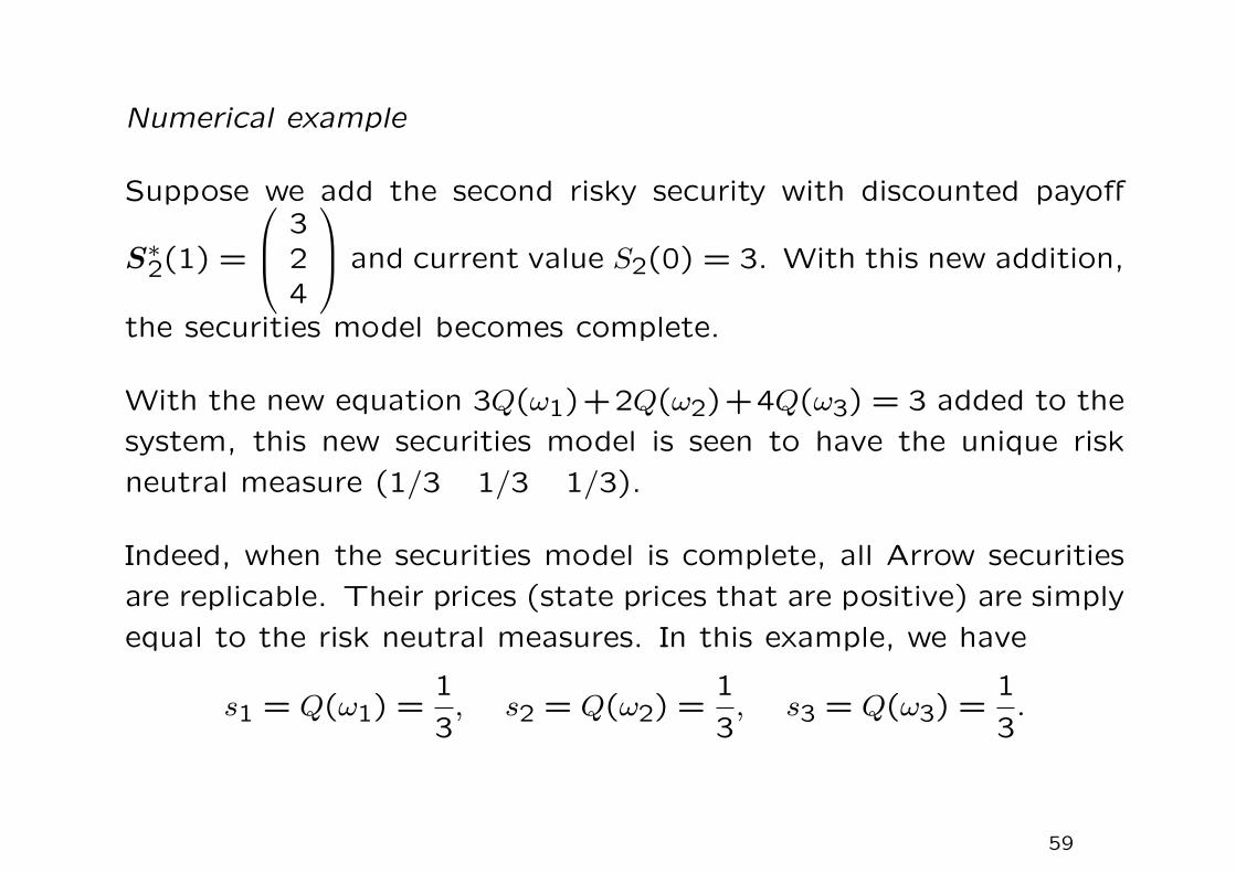
Numerical example

Suppose we add the second risky security with discounted payoff

S∗2(1) =

324

and current value S2(0) = 3. With this new addition,

the securities model becomes complete.

With the new equation 3Q(ω1)+2Q(ω2)+4Q(ω3) = 3 added to the

system, this new securities model is seen to have the unique risk

neutral measure (1/3 1/3 1/3).

Indeed, when the securities model is complete, all Arrow securities

are replicable. Their prices (state prices that are positive) are simply

equal to the risk neutral measures. In this example, we have

s1 = Q(ω1) =1

3, s2 = Q(ω2) =

1

3, s3 = Q(ω3) =

1

3.

59

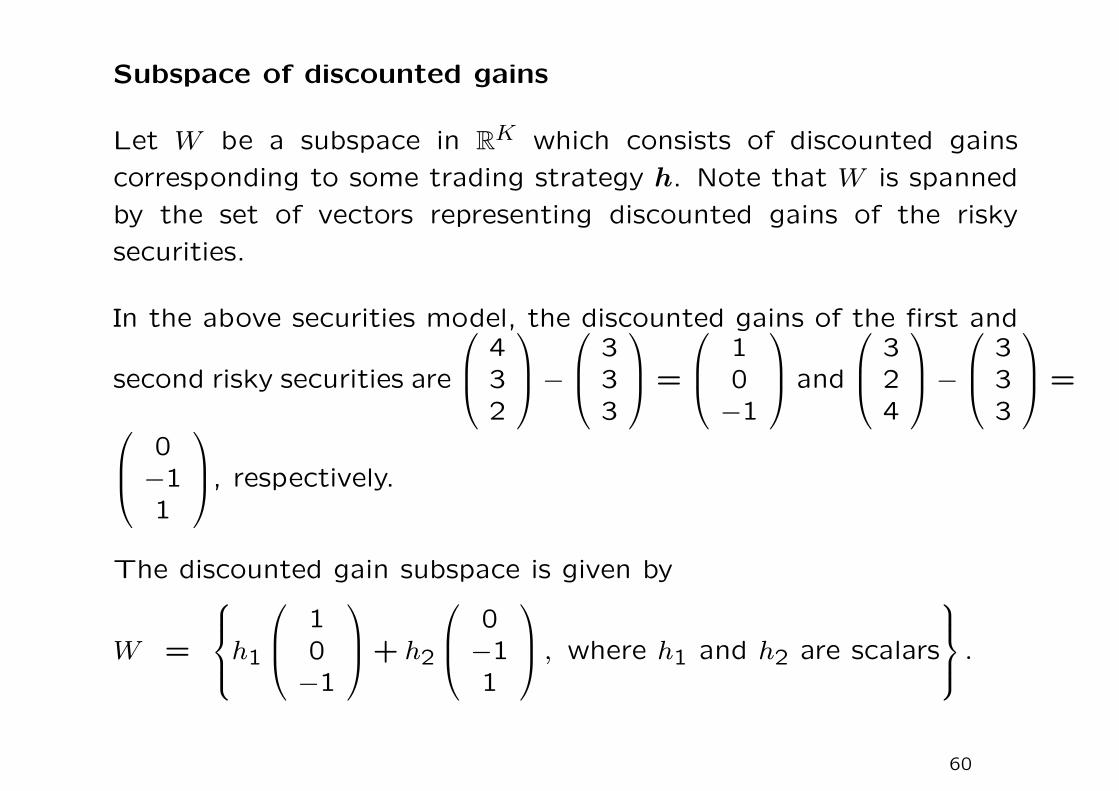
Subspace of discounted gains

Let W be a subspace in RK which consists of discounted gains

corresponding to some trading strategy h. Note that W is spanned

by the set of vectors representing discounted gains of the risky

securities.

In the above securities model, the discounted gains of the first and

second risky securities are

432

− 3

33

=

10−1

and

324

− 3

33

=

0−11

, respectively.

The discounted gain subspace is given by

W =

h1

10−1

+ h2

0−11

, where h1 and h2 are scalars

.

60

Orthogonality of the discounted gain vector and Q

Let G∗ denote the discounted gain of a portfolio. For any risk

neutral probability measure Q, we have

EQG∗ =

K∑k=1

Q(ωk)

M∑m=1

hm∆S∗m(ωk)

=

M∑m=1

hmEQ[∆S∗m] = 0.

Under the absence of arbitrage opportunities, the expected discount-

ed gain from any risky portfolio is simply zero. Apparently, there

is no risk premium derived from the risky investment. Therefore,

the financial economics term “risk neutrality” is adopted under this

framework of asset pricing.

For any G∗ = (G(ω1) · · ·G(ωK))T ∈W , we have

QG∗ = 0, where Q = (Q(ω1) · · ·Q(ωK)).

61

Characterization of the set of neutral measures

Since the sum of risk neutral probabilities must be one and all prob-

ability values must be positive, the risk neutral probability vector Q

must lie in the following subset

P+ = y ∈ RK : y1+y2+· · ·+yK = 1 and yk > 0, k = 1, · · ·K.

Also, the risk neutral probability vector Q must lie in the orthogonal

complement W⊥, where W is the discounted gain subspace. Let R

denote the set of all risk neutral measures, then R = P+ ∩W⊥.

In the above numerical example, W⊥ is the line through the origin

in R3 which is perpendicular to (1 0 −1) and (0 −1 1). The

line should assume the form λ(1 1 1) for some scalar λ. We

obtain the risk neutral probability vector Q = (1/3 1/3 1/3).

62

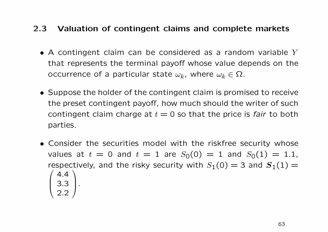
2.3 Valuation of contingent claims and complete markets

• A contingent claim can be considered as a random variable Y

that represents the terminal payoff whose value depends on the

occurrence of a particular state ωk, where ωk ∈ Ω.

• Suppose the holder of the contingent claim is promised to receive

the preset contingent payoff, how much should the writer of such

contingent claim charge at t = 0 so that the price is fair to both

parties.

• Consider the securities model with the riskfree security whose

values at t = 0 and t = 1 are S0(0) = 1 and S0(1) = 1.1,

respectively, and the risky security with S1(0) = 3 and S1(1) = 4.43.32.2

.

63

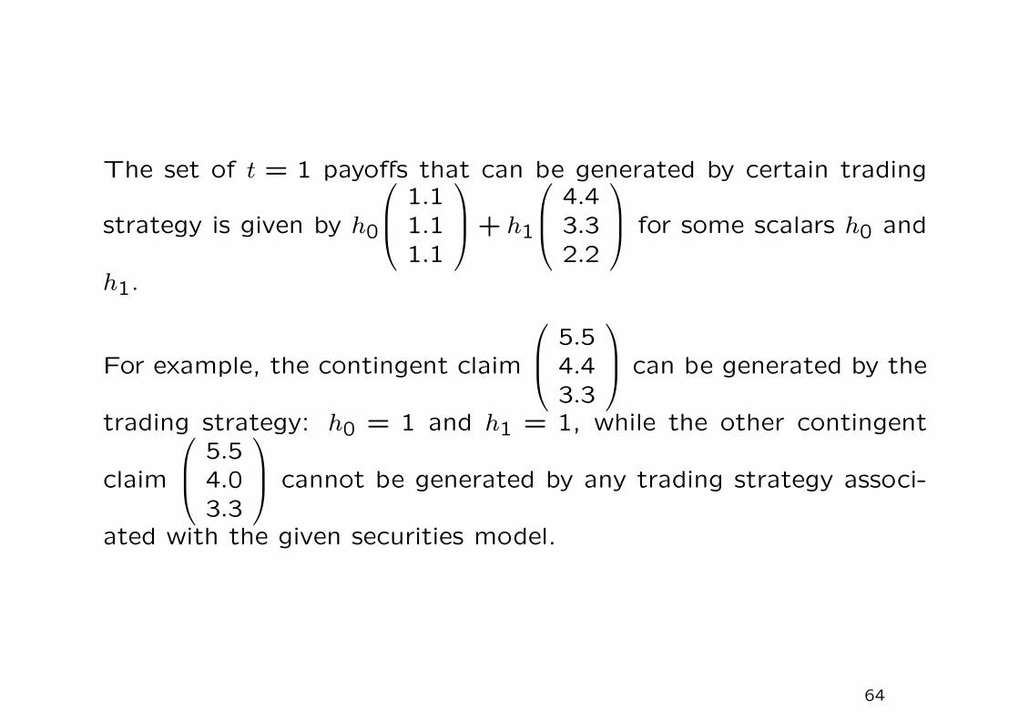
The set of t = 1 payoffs that can be generated by certain trading

strategy is given by h0

1.11.11.1

+ h1

4.43.32.2

for some scalars h0 and

h1.

For example, the contingent claim

5.54.43.3

can be generated by the

trading strategy: h0 = 1 and h1 = 1, while the other contingent

claim

5.54.03.3

cannot be generated by any trading strategy associ-

ated with the given securities model.

64

A contingent claim Y is said to be attainable if there exists some

trading strategy h, called the replicating portfolio, such that V1 = Y

for all possible states occurring at t = 1.

The price at t = 0 of the replicating portfolio is given by

V0 = h0S0(0) + h1S1(0) = 1× 1 + 1× 3 = 4.

Suppose there are no arbitrage opportunities (equivalent to the ex-

istence of a risk neutral probability measure), then the law of one

price holds and so V0 is unique.

65

Pricing of attainable contingent claims

Let V ∗1 (1; Ω) denote the discounted value of the replicating portfolio

that matches with the payoff of the attainable contingent claim at

every state of the world. Suppose the associated trading strategy

to generate the replicating portfolio is h, then

V ∗1 = S∗(1; Ω)h.

The initial cost of setting up the replicating portfolio is

V0 = S(0)h.

Assuming π exists, where S(0) = πS∗(1; Ω) so that

V0 = πS∗(1; Ω)h = πV ∗1 (1; Ω)

=K∑k=1

πkV∗

1 (1;ωk), independent of h.

Even when π is not a risk neutral measure or linear pricing measure,

the above pricing relation remains valid. Note that π may not be

unique, however we always have the same value for V0 by virtue of

law of one price.66

• Consider a given attainable contingent claim Y which is gen-

erated by certain trading strategy. The associated discounted

gain G∗ of the trading strategy is given by G∗ =M∑

m=1

hm∆S∗m.

Now, suppose a risk neutral probability measure Q associated

with the securities model exists, we have

V0 = EQV0 = EQ[V ∗1 −G∗].

Since EQ[G∗] = EQ[M∑

m=1

hm∆S∗m] =M∑

m=1

hmEQ[∆S∗m] = 0, and

V ∗1 = Y ∗ by virtue of replication. We obtain

V0 = EQ[Y ∗].

Risk neutral valuation principle:

The price at t = 0 of an attainable claim Y is given by the expec-

tation under any risk neutral measure Q of the discounted payoff of

the contingent claim.

67

Recall that the existence of the risk neutral probability measure

implies the law of one price. Provided that Y is attainable, EQ[Y ∗]assumes the same value for every risk neutral probability measure

Q by virtue of the law of one price. What happen to EQ[Y ∗] when

Y is non-attainable? We will show that EQ[Y ∗] does not take the

same value for all Q ∈M .

Theorem (Attainability of a contingent claim and uniqueness of

EQ[Y ∗])

Suppose the securities model admits no arbitrage opportunities.

The contingent claim Y is attainable if and only if EQ[Y ∗] takes

the same value for every Q ∈M , where M is the set of risk neutral

measures.

68

Proof

=⇒ part

existence of Q ⇐⇒ absence of arbitrage =⇒ law of one price. For

an attainable Y , EQ[Y ∗] is constant with respect to all Q ∈ M ,

otherwise this leads to violation of the law of one price.

⇐= part

It suffices to show that if the contingent claim Y is not attainable

then EQ[Y ∗] does not take the same value for all Q ∈M .

69

Let y∗ ∈ RK be the discounted payoff vector corresponding to Y ∗.Since Y is not attainable, then there is no solution to

S∗(1)h = y∗

(non-existence of trading strategy h). It then follows that there

exists a non-zero row vector π ∈ RK such that

πS∗(1) = 0 and πy∗ 6= 0.

Remark

Recall that the orthogonal complement of the column space is the

left null space. The dimension of the left null space equals K−column rank, and it is non-zero since the column space does not

span the whole RK. The above result indicates that when y∗ is not

in the column space of S∗(1), then there exists a non-zero vector π

in the left null space of S∗(1) such that y∗ and π are not orthogonal.

If otherwise, y∗ is orthogonal to every vector in the left null space,

then y∗ lies in the column space. This leads to a contradiction.

70

Write π = (π1 · · ·πK). Let Q ∈ M be an arbitrary risk neutral

measure, and let λ > 0 be small enough such that

Q(ωk) = Q(ωk) + λπk > 0, k = 1,2, · · · ,K.

To show that Q(ωk) is a risk neutral measure, it suffices to show

that Q satisfies

QS∗(1) = S(0).

Consider

QS∗(1) = QS∗(1) + λπS∗(1)

and observe that

QS∗(1) = S(0) and πS∗(1) = 0,

so the required condition is checked. Note that∑Kk=1Q(wk) = 1 is

satisfied since∑Kk=1 πk = 0 [as enforced by zero value of the product

of π with the first column of S∗(1)].

71

Lastly, we consider

EQ[Y ∗] =K∑k=1

Q(ωk)Y ∗(ωk)

=K∑k=1

Q(ωk)Y ∗(ωk) + λK∑k=1

πkY∗(ωk).

The last term is non-zero since πy∗ 6= 0 and λ > 0. Therefore, we

have

EQ[Y ∗] 6= EQ

[Y ∗].

Thus, when Y is not attainable, EQ[Y ∗] does not take the same

value for all risk neutral measures.

Corollary Given that the set of risk neutral measures R is non-

empty. The securities model is complete if and only if R consists of

exactly one risk neutral measure.

completeness of securities model ⇔ uniqueness of Q

72

An earlier proof of “=⇒ part” has been shown on p.59. Alter-

natively, we may prove by contradiction: non-uniqueness of Q ⇒non-completeness.

Suppose there exist two distinct Q and Q, that is, Q(ωk) 6= Q(ωk)

for some state ωk. Let Y ∗ =

1 if ω = ωk0 otherwise

, which is the kth Arrow

security. Obviously,

EQ[Y ∗] = Q(ωk) 6= Q(ωk) = EQ

[Y ∗],

so EQ[Y ∗] is not unique. By the theorem, the kth Arrow security is

not attainable so the securities model is not complete.

⇐= part: If the risk neutral measure is unique, then for any con-

tingent claim Y,EQ[Y ∗] takes the same value for any Q (actually

single Q). Hence, any contingent claim is attainable so the market

is complete.

73

Remarks

• When the securities model is complete and admits no arbitrage

opportunities, then all Arrow securities lie in the asset span and

risk neutral measures exist. The state price of state ωk exists

for any state and it is equal to the unique risk neutral probability

Q(ωk). The risk neutral valuation procedure can be applied for

pricing any contingent claim (which is always attainable due to

completeness).

• On the other hand, suppose there are two risk neutral probability

values for the same state ωk, the state price of that state cannot

be defined properly without contradicting the law of one price.

Actually, by the theorem, the Arrow security of that state would

not be attainable, so the securities model cannot be complete.

74

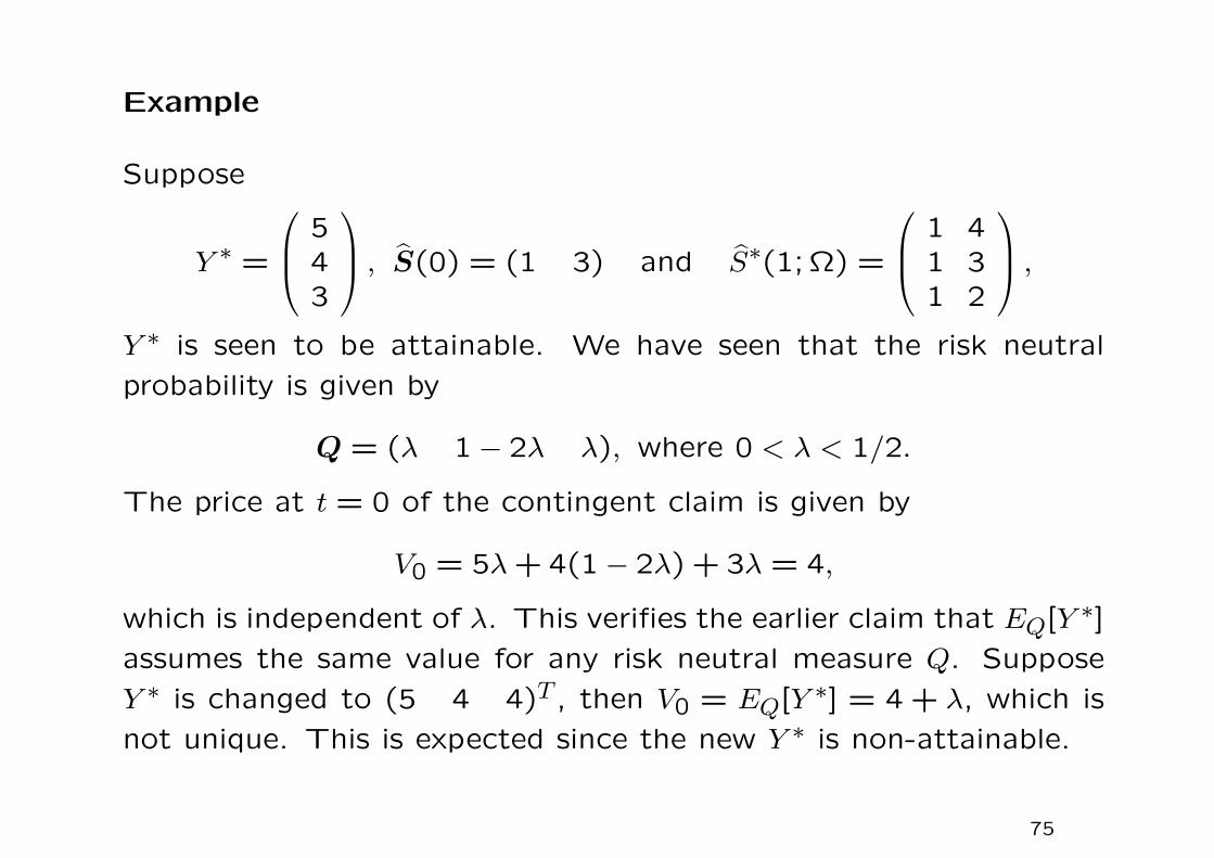
Example

Suppose

Y ∗ =

543

, S(0) = (1 3) and S∗(1; Ω) =

1 41 31 2

,Y ∗ is seen to be attainable. We have seen that the risk neutral

probability is given by

Q = (λ 1− 2λ λ), where 0 < λ < 1/2.

The price at t = 0 of the contingent claim is given by

V0 = 5λ+ 4(1− 2λ) + 3λ = 4,

which is independent of λ. This verifies the earlier claim that EQ[Y ∗]assumes the same value for any risk neutral measure Q. Suppose

Y ∗ is changed to (5 4 4)T , then V0 = EQ[Y ∗] = 4 + λ, which is

not unique. This is expected since the new Y ∗ is non-attainable.

75

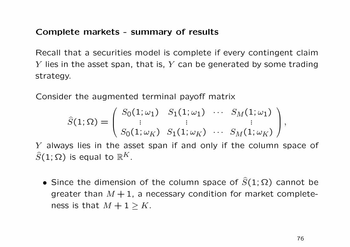
Complete markets - summary of results

Recall that a securities model is complete if every contingent claim

Y lies in the asset span, that is, Y can be generated by some trading

strategy.

Consider the augmented terminal payoff matrix

S(1; Ω) =

S0(1;ω1) S1(1;ω1) · · · SM(1;ω1)... ... ...

S0(1;ωK) S1(1;ωK) · · · SM(1;ωK)

,Y always lies in the asset span if and only if the column space of

S(1; Ω) is equal to RK.

• Since the dimension of the column space of S(1; Ω) cannot be

greater than M + 1, a necessary condition for market complete-

ness is that M + 1 ≥ K.

76

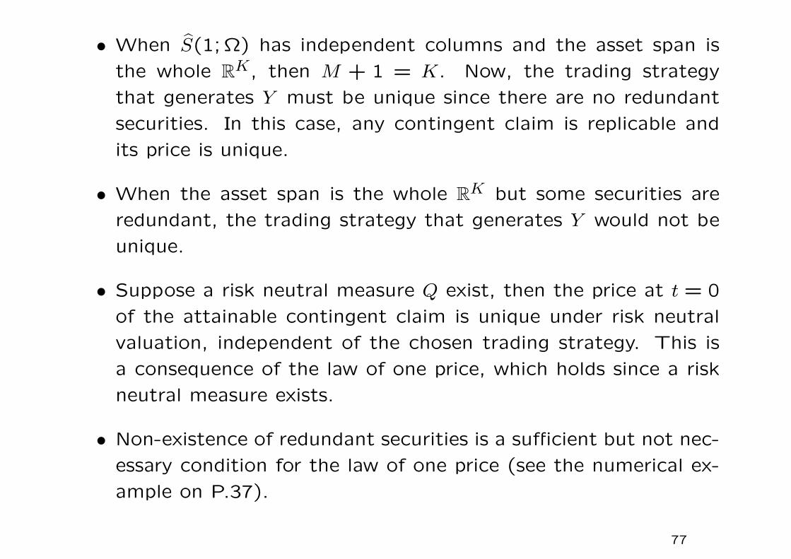
• When S(1; Ω) has independent columns and the asset span is

the whole RK, then M + 1 = K. Now, the trading strategy

that generates Y must be unique since there are no redundant

securities. In this case, any contingent claim is replicable and

its price is unique.

• When the asset span is the whole RK but some securities are

redundant, the trading strategy that generates Y would not be

unique.

• Suppose a risk neutral measure Q exist, then the price at t = 0

of the attainable contingent claim is unique under risk neutral

valuation, independent of the chosen trading strategy. This is

a consequence of the law of one price, which holds since a risk

neutral measure exists.

• Non-existence of redundant securities is a sufficient but not nec-

essary condition for the law of one price (see the numerical ex-

ample on P.37).

77

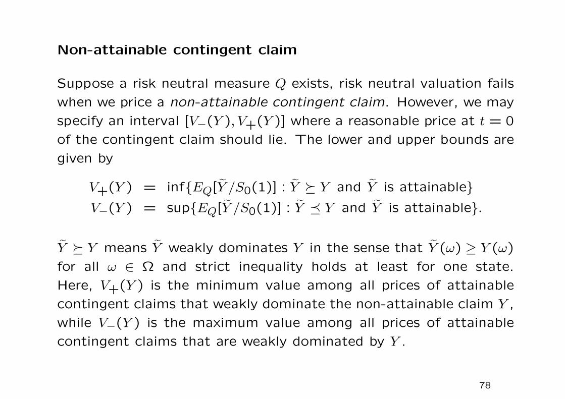
Non-attainable contingent claim

Suppose a risk neutral measure Q exists, risk neutral valuation fails

when we price a non-attainable contingent claim. However, we may

specify an interval [V−(Y ), V+(Y )] where a reasonable price at t = 0

of the contingent claim should lie. The lower and upper bounds are

given by

V+(Y ) = infEQ[Y /S0(1)] : Y Y and Y is attainableV−(Y ) = supEQ[Y /S0(1)] : Y Y and Y is attainable.

Y Y means Y weakly dominates Y in the sense that Y (ω) ≥ Y (ω)

for all ω ∈ Ω and strict inequality holds at least for one state.

Here, V+(Y ) is the minimum value among all prices of attainable

contingent claims that weakly dominate the non-attainable claim Y ,

while V−(Y ) is the maximum value among all prices of attainable

contingent claims that are weakly dominated by Y .

78

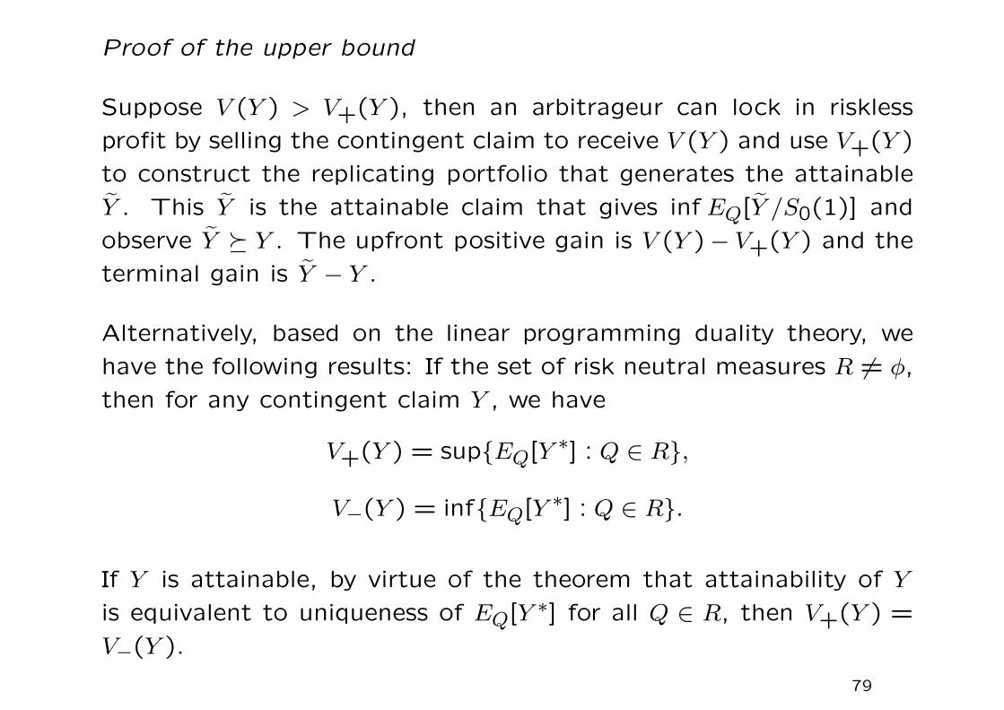
Proof of the upper bound

Suppose V (Y ) > V+(Y ), then an arbitrageur can lock in riskless

profit by selling the contingent claim to receive V (Y ) and use V+(Y )

to construct the replicating portfolio that generates the attainable

Y . This Y is the attainable claim that gives inf EQ[Y /S0(1)] and

observe Y Y . The upfront positive gain is V (Y )− V+(Y ) and the

terminal gain is Y − Y .

Alternatively, based on the linear programming duality theory, we

have the following results: If the set of risk neutral measures R 6= φ,

then for any contingent claim Y , we have

V+(Y ) = supEQ[Y ∗] : Q ∈ R,

V−(Y ) = infEQ[Y ∗] : Q ∈ R.

If Y is attainable, by virtue of the theorem that attainability of Y

is equivalent to uniqueness of EQ[Y ∗] for all Q ∈ R, then V+(Y ) =

V−(Y ).

79

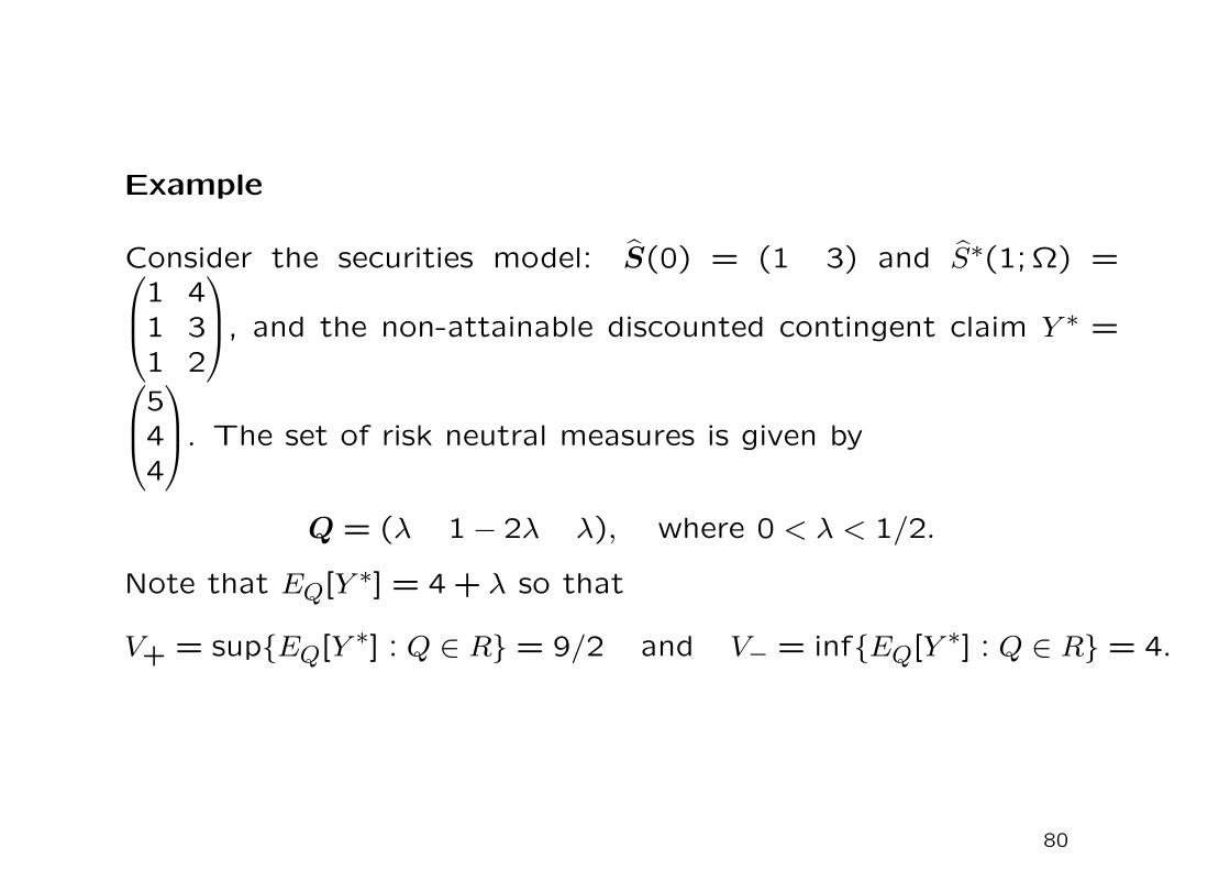
Example

Consider the securities model: S(0) = (1 3) and S∗(1; Ω) =1 41 31 2

, and the non-attainable discounted contingent claim Y ∗ =

544

. The set of risk neutral measures is given by

Q = (λ 1− 2λ λ), where 0 < λ < 1/2.

Note that EQ[Y ∗] = 4 + λ so that

V+ = supEQ[Y ∗] : Q ∈ R = 9/2 and V− = infEQ[Y ∗] : Q ∈ R = 4.

80

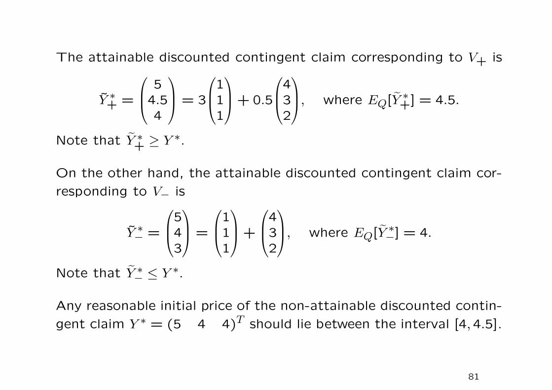
The attainable discounted contingent claim corresponding to V+ is

Y ∗+ =

54.54

= 3

111

+ 0.5

432

, where EQ[Y ∗+] = 4.5.

Note that Y ∗+ ≥ Y∗.

On the other hand, the attainable discounted contingent claim cor-

responding to V− is

Y ∗− =

543

=

111

+

432

, where EQ[Y ∗−] = 4.

Note that Y ∗− ≤ Y ∗.

Any reasonable initial price of the non-attainable discounted contin-

gent claim Y ∗ = (5 4 4)T should lie between the interval [4,4.5].

81

Summary Arbitrage opportunity

An arbitrage strategy is requiring no initial investment, having no

probability of negative value at expiration, and yet having some

possibility of a positive terminal portfolio value.

• It is commonly assumed that there are no arbitrage opportunities

in well functioning and competitive financial markets.

1. absence of arbitrage opportunities

⇒ absence of dominant trading strategies

⇒ law of one price

82

2. absence of arbitrage opportunities ⇔ existence of a risk neutral

measure

absence of dominant trading strategies ⇔ existence of a linear

pricing measure.

3. Provided that the securities model is complete and law of one

price holds, then state prices exist and single-valued. However,

state prices may be negative. The state prices are non-negative

when a linear pricing measure exists and they become strictly

positive when a risk neutral measure exists.

4. Under the absence of arbitrage opportunities, the risk neutral

valuation principle can be applied to find the fair price of an

attainable contingent claim. When the contingent claim is not

attainable, we can specify the range of prices that reasonable

prices should lie in order to avoid arbitrage opportunities.

83

2.4 Binomial option pricing models

By buying the underlying asset and shorting riskless money market

account in appropriate proportions, one can replicate the position

of a call.

Under the binomial random walk model, the asset price S∆t after

one period ∆t will be either uS or dS with probability q and 1 − q,respectively. Note that S∆t is a Bernoulli random variable that

assumes only two discrete values.

We assume u > 1 > d so that uS and dS represent the up-move and

down-move of the asset price, respectively. The jump parameters u

and d will be related to the asset price dynamics.

84

Let R denote the growth factor of riskless investment over one

period so that $1 invested in a riskless money market account will

grow to $R after one period. In order to avoid riskless arbitrage

opportunities, we must have u > R > d.

For example, suppose u > d > R, then we borrow as much as possible

for the riskfree asset and use the loan to buy the risky asset. Even

the downward move of the risky asset generates a return better than

the riskfree rate. This represents an arbitrage.

Suppose we form a portfolio which consists of α units of the asset

and cash amount M in the form of riskless money market account.

After one period 4t, the value of the portfolio becomesαuS +RM with probability qαdS +RM with probability 1− q.

85

Valuation of a call option using the approach of replication

The portfolio is used to replicate the long position of a call option

on a non-dividend paying asset.

As there are two possible states of the world: asset price goes up

or down, the call is thus a contingent claim.

Suppose the current time is only one period 4t prior to expiration.

Let c denote the current call price, and cu and cd denote the call

price after one period (which is the expiration time in the present

context) corresponding to the up-move and down-move of the asset

price, respectively.

86

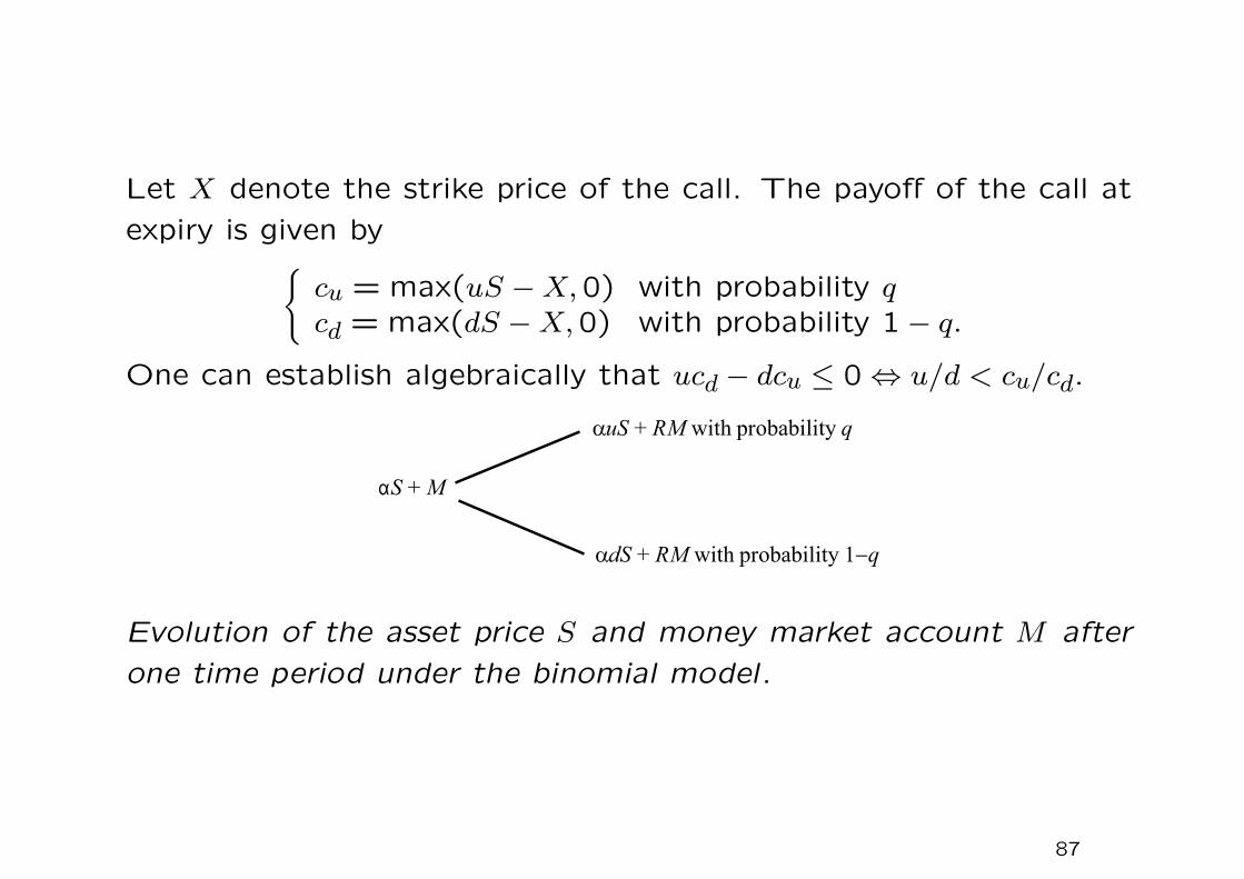
Let X denote the strike price of the call. The payoff of the call at

expiry is given bycu = max(uS −X,0) with probability qcd = max(dS −X,0) with probability 1− q.

One can establish algebraically that ucd − dcu ≤ 0⇔ u/d < cu/cd.

Evolution of the asset price S and money market account M after

one time period under the binomial model.

87

Concept of replication revisited

The above portfolio containing the risky asset and money market

account is said to replicate the long position of the call if and only

if the values of the portfolio and the call option match for each

possible outcome, that is,

αuS +RM = cu and αdS +RM = cd.

Solving the equations, we obtain

α =cu − cd

(u− d)S> 0, M =

ucd − dcu(u− d)R

< 0.

• Apparently, the binomial model is fortunate to have two instru-

ments in the replicating portfolio and two states of the world so

that the number of equations equals the number of unknowns.

The securities model is complete.

88

1. The parameters α and M are seen to have opposite sign since the

payoff of a call is long stock and short money market account.

2. u/d < cu/cd due to the leverage effect inherited in the call op-

tion. That is, when a given upside growth/downside drop is

experienced in the stock, the corresponding ratio is higher in

the call.

• The number of units of asset held is seen to be the ratio of the

difference of call values cu − cd to the difference of asset values

uS − dS. This ratio is called the hedge ratio.

• The call option can be replicated by a portfolio of the two ba-

sic securities: long risky asset and short riskfree money market

account.

89

Binomial option pricing formula

By no-arbitrage argument, the current value of the call is given by

the current value of the replicating portfolio, that is,

c = αS +M =R−du−d cu + u−R

u−d cdR

=pcu + (1− p)cd

Rwhere p =

R− du− d

.

This confirms with the risk neutral valuation principle under a risk

neutral measure.

• The probability q, which is the subjective probability about up-

ward or downward movement of the asset price, does not appear

in the call value. The parameter p can be shown to be 0 < p < 1

since u > R > d and so p can be interpreted as a probability.

90

Query Why not perform the simple discounted expectation proce-

dure using the subjective probabilities q and 1− q, where

c =qcu + (1− q)cd

R?

The relation

puS + (1− p)dS =R− du− d

uS +u−Ru− d

dS = RS

shows that the expected rate of returns on the asset with p as the

probability of upside move is just equal to the riskless interest rate:

S =1

RE∗[S∆t|S],

where E∗ is expectation under this probability measure. This relation

reveals that the asset price process is a martingale under the risk

neutral measure. We may view p as the risk neutral probability .

91

Treating the binomial model as a one-period securities model

The securities model consists of the riskfree asset and one risky asset

with initial price vector: S∗(0) = (1 S) and discounted terminal

payoff matrix: S∗(1) =

(1 uS

R1 dS

R

).

The risk neutral probability measure Q(ω) = (Q(ωu) Q(ωd)) is ob-

tained by solving

(Q(ωu) Q(wd))

(1 uS

R1 dS

R

)= (1 S).

We obtain

Q(ωu) = 1−Q(ωd) =R− du− d

.

The securities model is complete since there are two states and two

securities. Provided that the securities model admits no arbitrage

opportunities, we have uniqueness of the risk neutral measure.

92

Condition on u, d and R for absence of arbitrage

The set of risk neutral measures is given by R = P+∩W⊥, where W

is the subspace of discounted gains. In the binomial random walk

model, W is spanned by the single vector

(uR − 1dR − 1

)S since there is

only one risky asset. Knowing that u > d, the no arbitrage condition:

u > R > d is equivalent to

u

R− 1 > 0 and

d

R− 1 < 0 ⇔ u > R > d

To derive the above “no-arbitrage” condition using geometrical in-

tuition, a vector normal to

(uR − 1dR − 1

)S lies in the first quadrant of

Q(ωu)-Q(ωd) plane if and only if u > R > d.

By risk neutral valuation formula, we have

c =Q(ωu)cu +Q(ωd)cd

R=

1

RE∗[c∆t|S].

93

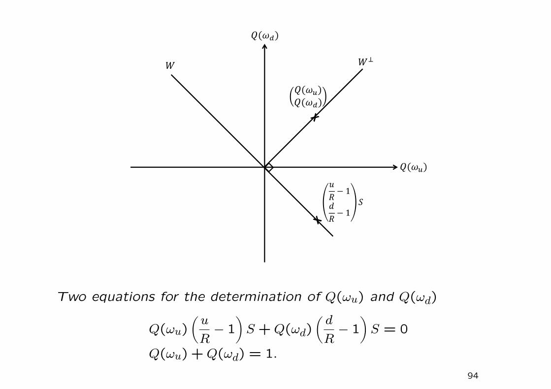
Two equations for the determination of Q(ωu) and Q(ωd)

Q(ωu)(u

R− 1

)S +Q(ωd)

(d

R− 1

)S = 0

Q(ωu) +Q(ωd) = 1.

94

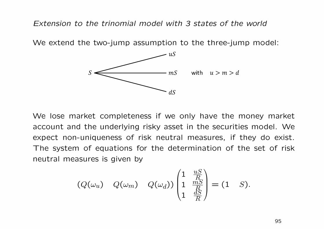
Extension to the trinomial model with 3 states of the world

We extend the two-jump assumption to the three-jump model:

We lose market completeness if we only have the money market

account and the underlying risky asset in the securities model. We

expect non-uniqueness of risk neutral measures, if they do exist.

The system of equations for the determination of the set of risk

neutral measures is given by

(Q(ωu) Q(ωm) Q(ωd))

1 uS

R1 mS

R1 dS

R

= (1 S).

95

Summary

• The binomial call value formula can be expressed by the following

risk neutral valuation formulation:

c =1

RE∗[c∆t|S],

where c denotes the call value at the current time, and c∆t de-

notes the random variable representing the call value one period

later. The call price can be interpreted as the expectation of

the payoff of the call option at expiry under the risk neutral

probability measure E∗ discounted at the riskless interest rate.

• Since there are 3 states of the world in a trinomial model, the

application of the principle of replication of claims fails to derive

the trinomial option pricing formula. Alternatively, one may use

the risk neutral valuation approach via the determination of the

risk neutral measures.

96

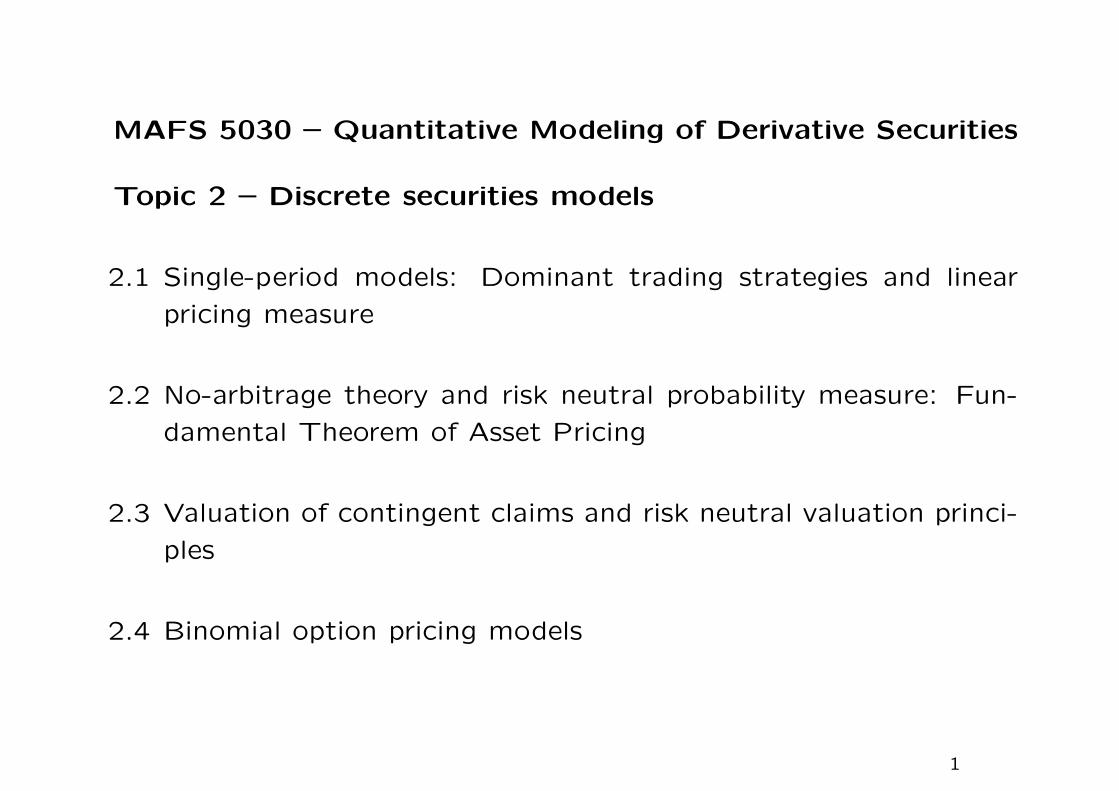
Multiperiod binomial models

Let cuu denote the call value at two periods beyond the current time

with two consecutive upward moves of the asset price and similar

notational interpretation for cud and cdd. The call values cu and cdare related to cuu, cud and cdd as follows:

cu =pcuu + (1− p)cud

Rand cd =

pcud + (1− p)cddR

.

The call value at the current time which is two periods from expiry

is found to be

c =p2cuu + 2p(1− p)cud + (1− p)2cdd

R2,

where the corresponding terminal payoff values are given by

cuu = max(u2S−X,0), cud = max(udS−X,0), cdd = max(d2S−X,0).

97

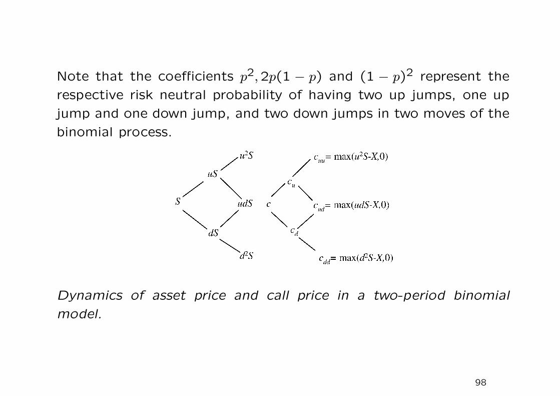
Note that the coefficients p2,2p(1 − p) and (1 − p)2 represent the

respective risk neutral probability of having two up jumps, one up

jump and one down jump, and two down jumps in two moves of the

binomial process.

Dynamics of asset price and call price in a two-period binomial

model.

98

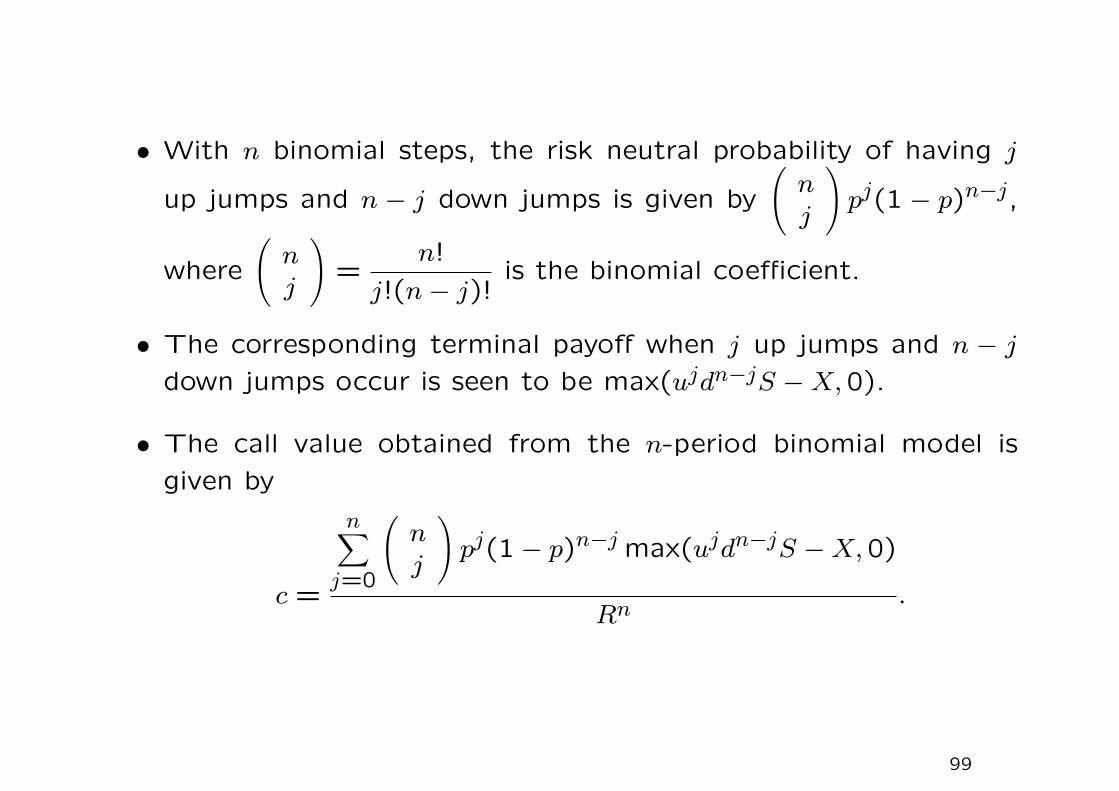
• With n binomial steps, the risk neutral probability of having j

up jumps and n − j down jumps is given by

(nj

)pj(1 − p)n−j,

where

(nj

)=

n!

j!(n− j)!is the binomial coefficient.

• The corresponding terminal payoff when j up jumps and n − jdown jumps occur is seen to be max(ujdn−jS −X,0).

• The call value obtained from the n-period binomial model is

given by

c =

n∑j=0

(nj

)pj(1− p)n−j max(ujdn−jS −X,0)

Rn.

99

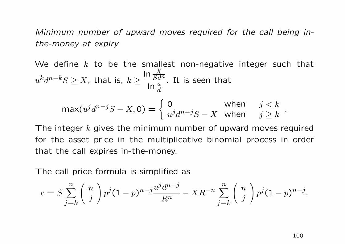
Minimum number of upward moves required for the call being in-

the-money at expiry

We define k to be the smallest non-negative integer such that

ukdn−kS ≥ X, that is, k ≥ln XSdn

ln ud

. It is seen that

max(ujdn−jS −X,0) =

0 when j < k

ujdn−jS −X when j ≥ k .

The integer k gives the minimum number of upward moves required

for the asset price in the multiplicative binomial process in order

that the call expires in-the-money.

The call price formula is simplified as

c = Sn∑

j=k

(nj

)pj(1− p)n−j

ujdn−j

Rn−XR−n

n∑j=k

(nj

)pj(1− p)n−j.

100

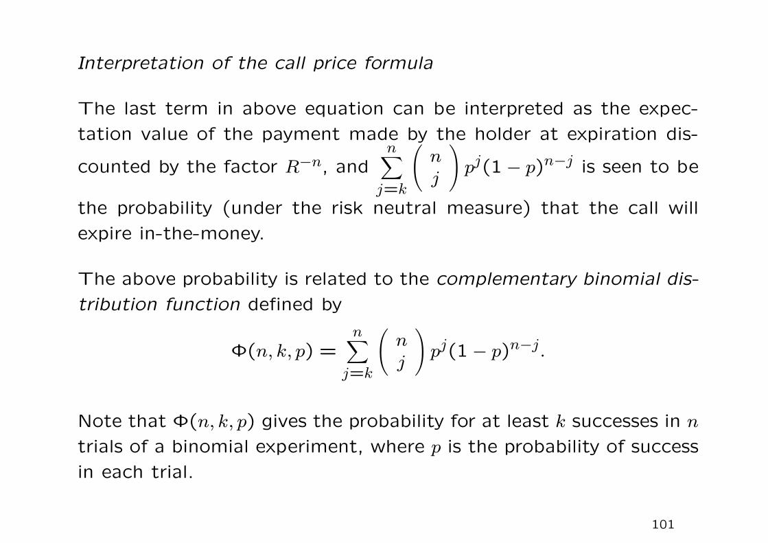
Interpretation of the call price formula

The last term in above equation can be interpreted as the expec-

tation value of the payment made by the holder at expiration dis-

counted by the factor R−n, andn∑

j=k

(nj

)pj(1− p)n−j is seen to be

the probability (under the risk neutral measure) that the call will

expire in-the-money.

The above probability is related to the complementary binomial dis-

tribution function defined by

Φ(n, k, p) =n∑

j=k

(nj

)pj(1− p)n−j.

Note that Φ(n, k, p) gives the probability for at least k successes in n

trials of a binomial experiment, where p is the probability of success

in each trial.

101

Further, if we write p′ =up

Rso that 1− p′ =

d(1− p)

R, then the call

price formula for the n-period binomial model can be expressed as

c = SΦ(n, k, p′)−XR−nΦ(n, k, p).

Alternatively, from the risk neutral valuation principle, we have

c =1

RnEQ

[ST1ST>X

]−X

RnEQ

[1ST>X

].

• The first term gives the discounted expectation of the asset

price at expiration given that the call expires in-the-money.

• The second term gives the present value of the risk neutral

expectation of payment incurred conditional on the call being

in-the-money at expiry.

102