Macroscopic modeling of traffic in cities final · Macroscopic modeling of traffic in cities By Nikolas Geroliminis* Institute of Transportation Studies University of California,

Macroscopic modeling of traffic in cities

By

Nikolas Geroliminis* Institute of Transportation Studies University of California, Berkeley

416D McLaughlin Hall, Berkeley, CA 94720-1720 Phone: (510) 643-2310, Fax: (510) 642-1246

E-mail: [email protected]

and

Carlos F. Daganzo Institute of Transportation Studies University of California, Berkeley

416A McLaughlin Hall, Berkeley, CA 94720-1720 Phone: (510) 642-3853, Fax: (510) 642-1246

E-mail: [email protected]

For Presentation 86th Annual Meeting

Transportation Research Board Washington, D.C.

January 2007

*corresponding author

Geroliminis and Daganzo 1

ABSTRACT

Most of the existing models for large scale arterial networks are not realistic and appropriate to deal with crowded conditions. As an alternative, we propose observation-based models that circumvent the fragility problems of traditional models. Monitoring replaces prediction, and the system is repeatedly modified based on observations. To succeed this goal a city is modeled in an aggregated manner and relations between traffic variables are developed. Macroscopic feedback control strategies are introduced which rely on real-time observation of relevant spatially aggregated measures of traffic performance. The proposed ideas are tested by simulation, while field experiments are in progress.

Keywords: macroscopic, control, gridlock, traffic, accumulation


INTRODUCTION Traffic congestion is increasing in major cities. The Texas Transportation Institute (1) estimated that in 2000 the 75 largest US metropolitan areas experienced 3.6 billion vehicle-hours of delay, resulting in 5.7 billion gallons in wasted fuel and $67.5 billion in lost productivity. Furthermore, between 1980 and 1999, the total length of roads in the United States increased by only 1.5 percent, while the total number of miles of vehicle travel increased by 76 percent (2). The construction of new infrastructure is not a feasible solution to decrease congestion, not only because of the tremendous cost to keep pace with population increases and the resulting increase in travel demand, but also because of the phenomenon of induced demand (3). From the above, it is perceivable that to decrease congestion in large cities and improve urban mobility we have to focus on the better utilization of the existing infrastructure. The development and evaluation of transportation policies for mobility improvements in cities around the world relies heavily on forecasting models (4). Given correct inputs, recent sophisticated models can predict much valuable information in disaggregate basis (link flows, travel time in each route etc) on a large transportation network. The problem with this approach is that, when dealing with congested systems, prediction-based evaluation models turn out to be quite fragile. Firstly, these models require disaggregated time-dependent origin-destination (O-D) tables. But for a model with a reasonable spatio-temporal resolution the required entries of the time dependent O-D tables are sufficiently large and in some cases greater than the whole population of a city. For example, a metropolitan area with 4 million people could be modeled with 400 zones (approximately 10000 people per zone). To model the morning and evening peak hour in 24 time intervals the total number of entries would have to be almost equal to the population of the city. But even if we were able to predict this huge amount of input information, performance measures such as total vehicle hours of travel for congested networks would be hard to predict because the outputs of congested systems are hyper-sensitive to the inputs. Small perturbations to the O-D tables or small changes to drivers’ route choices can drastically change the aggregate outputs (5). Most of the existing models for large scale arterial networks are not realistic and appropriate to deal with crowded conditions. As an alternative we propose following (4) to develop observation-based models that circumvent the fragility problems of traditional models. In this proposed approach, monitoring replaces prediction, and the system is repeatedly modified based on observations. To succeed this goal a city is modeled at an aggregated manner and relations between state variables are developed. Macroscopic feedback control strategies are introduced which rely on real-time observation of relevant spatially aggregated measures of traffic performance. The proposed ideas are tested by simulation, while field experiments are in progress. There are some examples of cities around the world, where macroscopic control strategies have been applied. A novel traffic light operating system designed for active management of the high


demand central area was developed and set up in Zurich. The traffic lights are internally coordinated based on the logic that the flow towards an overloaded area should be restricted while the flow towards an underutilized area should be promoted. Prevention of overcrowding on the city centre is achieved by metering of access to maintain the mobility of cars at a stabilized level. For example, longer red times are applied in the periphery of the centre during peak hours for phases which direct vehicles to the centre (6). A Congestion Charging Scheme was introduced in central London, covering 22 km2, in 2003. The main aims of the scheme are to reduce traffic congestion in and around the charging zone, to improve the bus services, journey time reliability for car users and to make the distribution of goods and services more reliable, sustainable and efficient. The reductions in both traffic and congestion that had been observed in the charging zone are around 30 percent. There are 65,000 fewer car trips into or through the zone per charging day as result of the scheme. The reliability of buses in and around the charging zone had also improved significantly (7). The remainder of the paper is organized as follows: First, we briefly review macroscopic models for arterial networks and present the study sites used in the paper. The next section describes macroscopic relations between traffic variables for a single link. The following section presents macroscopic relations in larger networks. The penultimate section describes dynamics and control of a two reservoir system while the last section presents findings and conclusions. BACKGROUND Early work by Wardrop (8) and Smeed (9) dealt with the development of macroscopic models for arterials, which were later extended to general networks. Smeed (10) modeled the number of vehicles which can enter the central area of a city as a function of the area of the town, the fraction of area devoted to roads and the capacity, expressed in vehicles per unit time per unit width of road. Thomson (11) used data from central London to develop a linear speed-flow model. Wardrop (12) developed a similar relation between average speed and flow by directly incorporating average street width and average signal spacing into his model. Zahavi (13) developed relations for different regions in different cities between traffic intensity (distance traveled per unit area), road density (length or area of roads per unit area), and weighted space mean speed using data from England and the United States. All of the described models are quite site specific and cannot be readily applied to other environments. A helpful work which establishes macroscopic relations in vehicular traffic in large cities is the two-fluid model of town traffic by Herman and Prigogine (14). The authors assumed that the speed distribution splits into two parts; one part corresponding to moving vehicles and the other to the vehicles that are stopped due to local conditions as congestion, traffic control devices, accidents etc., but not parked cars since there are not components of the moving traffic. The basic postulate of the theory relates the average speed of the moving vehicles vr, to the fraction of moving vehicles, fr as follows:

kr m rv v f= ⋅ , (1)


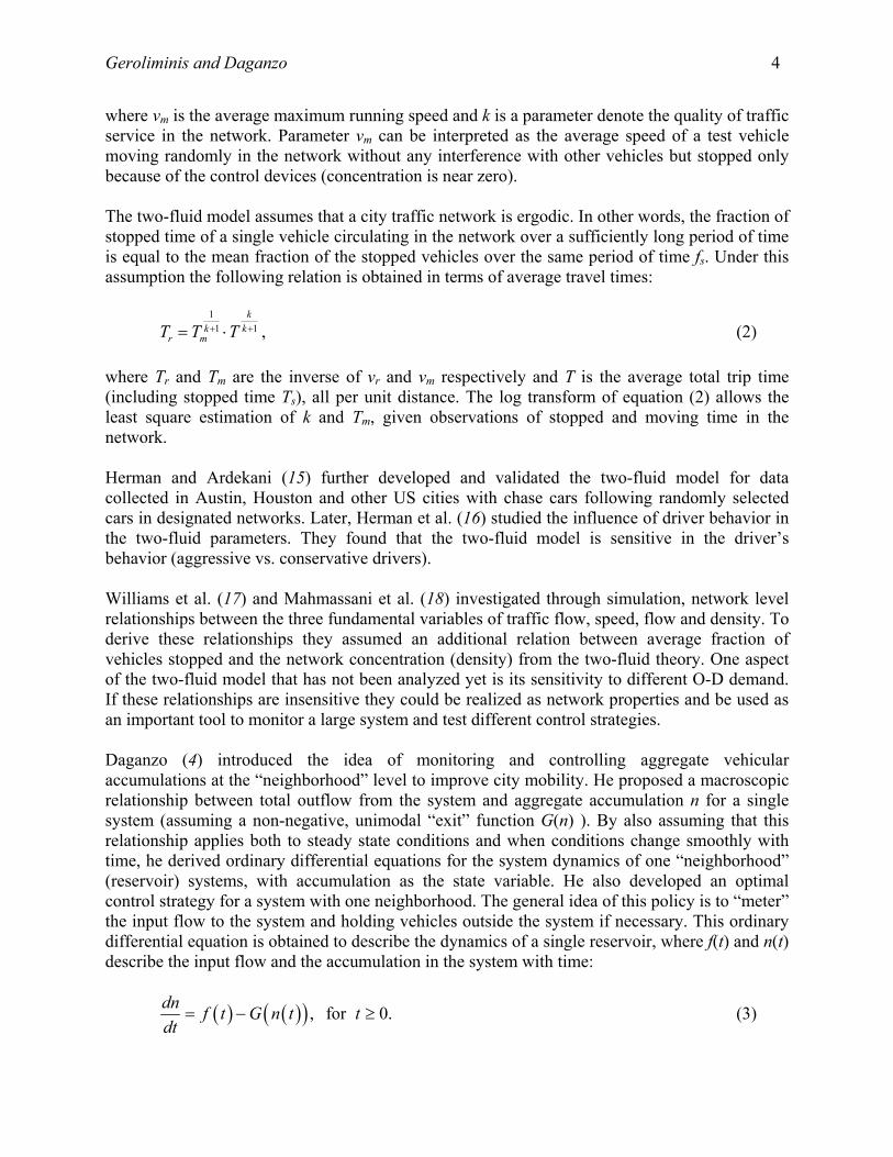
where vm is the average maximum running speed and k is a parameter denote the quality of traffic service in the network. Parameter vm can be interpreted as the average speed of a test vehicle moving randomly in the network without any interference with other vehicles but stopped only because of the control devices (concentration is near zero). The two-fluid model assumes that a city traffic network is ergodic. In other words, the fraction of stopped time of a single vehicle circulating in the network over a sufficiently long period of time is equal to the mean fraction of the stopped vehicles over the same period of time fs. Under this assumption the following relation is obtained in terms of average travel times:

11 1

kk k

r mT T T+ += ⋅ , (2) where Tr and Tm are the inverse of vr and vm respectively and T is the average total trip time (including stopped time Ts), all per unit distance. The log transform of equation (2) allows the least square estimation of k and Tm, given observations of stopped and moving time in the network.

Herman and Ardekani (15) further developed and validated the two-fluid model for data collected in Austin, Houston and other US cities with chase cars following randomly selected cars in designated networks. Later, Herman et al. (16) studied the influence of driver behavior in the two-fluid parameters. They found that the two-fluid model is sensitive in the driver’s behavior (aggressive vs. conservative drivers). Williams et al. (17) and Mahmassani et al. (18) investigated through simulation, network level relationships between the three fundamental variables of traffic flow, speed, flow and density. To derive these relationships they assumed an additional relation between average fraction of vehicles stopped and the network concentration (density) from the two-fluid theory. One aspect of the two-fluid model that has not been analyzed yet is its sensitivity to different O-D demand. If these relationships are insensitive they could be realized as network properties and be used as an important tool to monitor a large system and test different control strategies. Daganzo (4) introduced the idea of monitoring and controlling aggregate vehicular accumulations at the “neighborhood” level to improve city mobility. He proposed a macroscopic relationship between total outflow from the system and aggregate accumulation n for a single system (assuming a non-negative, unimodal “exit” function G(n) ). By also assuming that this relationship applies both to steady state conditions and when conditions change smoothly with time, he derived ordinary differential equations for the system dynamics of one “neighborhood” (reservoir) systems, with accumulation as the state variable. He also developed an optimal control strategy for a system with one neighborhood. The general idea of this policy is to “meter” the input flow to the system and holding vehicles outside the system if necessary. This ordinary differential equation is obtained to describe the dynamics of a single reservoir, where f(t) and n(t) describe the input flow and the accumulation in the system with time:

( ) ( )( ) , for 0.dn f t G n t tdt

= − ≥ (3)


This paper tries to build on these ideas and develop and validate a macroscopic approach to increase city mobility by controlling overcrowding. THE STUDY SITES The proposed ideas are validated by simulation in two arterial test sites: The Lincoln Avenue in Los Angeles and Downtown San Francisco Area. The first site is typical of one dimensional multilane major arterials on urban/suburban areas; the second site is a two dimensional network with varying geometric characteristics. i. Major Arterial: This test site is 1.42 mile long stretch of a major urban arterial (Lincoln

Avenue) north of the Los Angeles International Airport, between Fiji Way and Venice Boulevard in the cities of Los Angeles and Santa Monica. The study section includes 7 signalized intersections with link lengths varying from 500 to 1,600 feet. The number of lanes for through traffic per link is three lanes per direction for the length of the study area. Additional lanes for turning movements are provided at intersection approaches. The free flow speed is 40 mph. Traffic signals are all multiphase operating as coordinated under traffic responsive control. System cycle lengths range from 100 seconds early in the analysis period (6:00 to 6:30 am) to a maximum of 150 sec during the periods of highest traffic volume (7:30 to 8:30 am).

ii. Downtown City Center: This test site is a 2.5 square mile area of Downtown San Francisco

(Financial District and South Of Market Area), including about 100 intersections with link lengths varying from 400 to 1,300 feet. The number of lanes for through traffic varies from 2 to 5 lanes and the free flow speed is 30 miles per hour. Traffic signals are all multiphase fixed-time operating on a common cycle length of 100 seconds for the west boundary of the area (The Embarcadero) and 60 seconds for the rest.

Data on the study networks, geometrics and traffic volumes were available from previous research studies on traffic control. MACROSCOPIC RELATIONS FOR A SINGLE LINK It is difficult to understand traffic in large cities on a purely microscopic basis. But, despite the intense complexity of these systems, it is believed that the examination of relations among averages of pertinent variables in a macroscopic approach will lead to some functional dependence as a consequence of collective effects. The selection of the traffic variables which could describe macroscopically a large comparable to a link traffic system must be consistent with these criteria:

• The variables should describe realistically the physics of overcrowding • The variables should be highly correlated with the performance of the system. • The variables should be collected directly from field measurements and not be filtered

through models.


First, let’s introduce some traffic variables for a single homogeneous link with a signal at its downstream end and examine relations between them. Later, we will be able to describe the reasons these variables can satisfy the above criteria in an aggregated manner.

• Accumulation ni(t): The number of vehicles traveling in a link i at time t (excluding the parked vehicles) – (unit: vehicles)

• Travel Production Pi(t, t+∆t): The total distance traveled from all the vehicles traveling in a link between time t and t+∆t (unit: vehicle-meters)

• Output ei(t): The rate at which destinations along the link (or at its end) are being reached (unit: vehicles per time unit).

It is possible to calculate average quantities of these variables for periods comparable with a few cycles. The reason for this aggregation with time is to smooth the variations of traffic during a cycle: Congested conditions are developed near the stop line during the red interval, capacity conditions are observed in the period during which the queue is discharging at the saturation flow rate, and free flow conditions occur for the rest of the cycle. Kinematic wave traffic theory shows that travel production for a cycle is related to accumulation during steady state conditions by a trapezoidal relation such as the one shown by the dark lines of figure 1. Travel production has been normalized in such a way that slopes in this diagram have units of speed (L is the length of the link and C the cycle). Three different regimes are clear in the figure. Regime I (travel production increases with accumulation) represents undersaturated states where queues are transient and the total number of vehicles served is smaller than the maximum possible. These states are contained in the shaded wedge OAB. Line OA (a best case) consists of production – accumulation pairs for which all the vehicles arrive during the green phase and are served from the link with zero delay traveling at free flow speed vf. Line OB (the worst case) represents pairs with the maximum delay possible under undersaturated conditions. Since this delay is r (the length of red phase) the average (worst case) speed u is:

1 1

f

ru v L= + . (4)

Regime II (line AC in figure 1) represents saturated states. The link is filled part way with permanent queues and demand equals capacity. There is a limit to accumulation (point C) corresponding to queues that fill the link. In this regime travel production is constant and equal to L g s⋅ ⋅ , where g is the duration of green phase and s the saturation flow of the signal.

Regime III (production decreases with accumulation) corresponds to oversaturated states and the whole link is queued. They cannot arise by increasing the input flow; a restriction from downstream is necessary, for example if queues from downstream links block the departures during the green phase. Regime III consists of states where queues fill the link, vehicles are stopped or moving at saturation flow s.

According to Edie’s definitions (19) the mean flow q̂ (density k̂ ) of vehicles traveling over a link of length L during a time T is the total distance (time) traveled by all vehicles which were on


it during any part of time T divided by L×T, the area of the space-time domain observed. We prove that the rate mean flow (equal to production over L×C) decreases with mean density (equal to mean accumulation over L) is equal to the congested wave speed w of the fundamental triangular flow-density diagram. If gr<g is the duration of the real green time because of the downstream restriction, mean flow q̂ and mean density k̂ are:

1ˆ s rsq A s g

L C C= ⋅ ⋅ = ⋅

⋅ (5a)

( ) /1ˆ j fs s j j j r

k s vk A k A k k g

L C C−

= ⋅ ⋅ + ⋅ = − ⋅⋅

(5b)

where s rA L g= ⋅ and ( )j rA L C g= ⋅ − are the areas of the space-time where vehicles are observed at saturation density ks=s/vf and jam density kj respectively during a cycle C. The first derivative of mean flow with respect to mean density is:

ˆ ˆˆ ˆ /

r

r j f

dgdq dq s wdg k s vdk dk

= ⋅ = − = −−

(6)

Figure 1: Travel production vs. accumulation for a single link under steady state conditions

During transition from regime I or II to III non steady states can be observed which do not belong to any of the regimes (for example transition from D to E). Figure 2 shows a sequence of travel production and accumulation pairs averaged over two cycles for 3 different links of the second study site during a run with time dependent demand. Values have been normalized for illustration purposes. It is clear that transitions between points in the steady state regimes occur by following different paths, but one can discern the trapezoidal edge of these paths.

A B C D

O ni / L

Pi

uf w

u

L×C Fundamental Diagram

Restricted capacity E

, ei


0.00

0.10

0.20

0.30

0.40

0.50

0.60

0.00 0.02 0.04 0.06 0.08 0.10 0.12 0.14 0.16 0.18 0.20

accumulation /( Length * Lanes)

Trav

el P

rodu

ctio

n /(

Leng

th *

Lane

s * G

reen

) (610, 139)

(154, 626)

(609, 610)

Figure 2: Successive points of normalized travel production and accumulation

for individual links in the San Francisco network MACROSCOPIC RELATIONS FOR NETWORKS The big conjecture is that if a network is (roughly) homogeneously loaded and congestion is (roughly) evenly distributed over the network, then its production P measures under steady state conditions is the sum of the measures for individual links and can be expressed as a function of the total accumulation of the network independently of the disaggregate link data:

( ) ( )i i i iP P Q n Q n= = ≅∑ ∑ ∑ , (7) where Qi is the travel production function for the individual link i and Q for the aggregated quantities over the network. The quality of this approximation is an experimental issue. We also claim that the aggregated output O (number of vehicles finishing their trips per time unit) under steady state conditions is a function of the total accumulation Σni. Note that their ratio O/P is the reciprocal of average trip length L for all the vehicles traveling in the network. If n is the number of vehicles in a system; τ is the mean service time; v is the average speed; λ is the average entering rate and o is the average exit rate, then according to Little’s formula for steady state conditions (λ=ο) we have that n λ τ= ⋅ . Production P and outflow O for an interval ∆t are P n v t= ⋅ ⋅∆ and O o t= ⋅∆ respectively and their ratio O/P is:

1O o o

P n v v Lλ τ= = =

⋅ ⋅ ⋅ (8)

One important point is that accumulation and travel production are observable quantities, but output is not; as technologies do not exist to measure the rate vehicles finish their trips. Next section gives evidence that output and travel production are linearly related as per (8).


Simulation evidence i. Major Arterial Traffic was simulated in the first study site with CORSIM microscopic simulation model (20) for two periods of 4 hours, the morning and evening peak. Traffic demand changed every 15 minutes. Vehicle-miles travelled (VMT) and vehicle-hours travelled (VHT) every 15 seconds were recorded. VMT and VHT data were aggregated every two cycles and travel production and accumulation calculated. To test the sensitivity of the relation between production or outflow and accumulation, different O-D tables were used by changing the turning movements in each of the intersections, and the input flows of the major arterial. Figure 3a shows how travel production changes with accumulation. It is clear that equation 7 holds approximately. The three different regimes are clearly noticeable. For pairs in regime I, individual links are in regimes I and II of figure 1. For pairs in regime II (aggregated) most of the links operate at capacity, while in regime III (aggregated) individual links are in regimes II and III of figure 1. Congestion would be unevenly distributed over the network if individual links in regimes I and III persisted simultaneously. This would create points beneath the curve of figure 3a. Figure 3b shows total outflow (output) and production pairs for the major arterial network. They are linearly related. This suggests that the (observable) traffic production and average traffic speed are good proxies for the (unobservable) aggregate output.

0

90000

180000

270000

360000

450000

0 200 400 600 800 1000

accumulation (vhs)

Trav

el P

rodu

ctio

n (v

h-m

eter

s pe

r 2 c

ycle

s)

Figure 3a: Travel production vs. accumulation for Lincoln Ave., LA

Regime I

Regime II

Regime III


Outflow = (1/1760)* Travel ProductionR2 = 0.98

0

50

100

150

200

250

0 90000 180000 270000 360000 450000

Travel Production (vh-meters per 2 cycles)

outfl

ow (v

hs p

er 2

cyc

les)

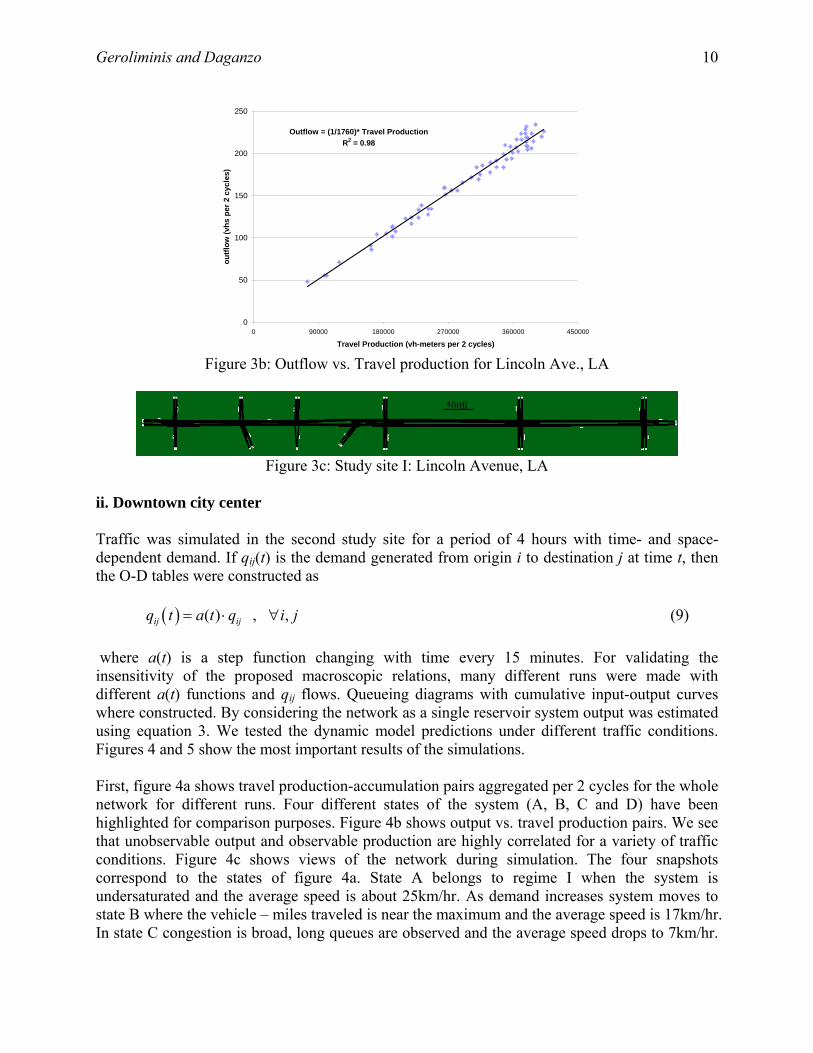
Figure 3b: Outflow vs. Travel production for Lincoln Ave., LA

Figure 3c: Study site I: Lincoln Avenue, LA

ii. Downtown city center Traffic was simulated in the second study site for a period of 4 hours with time- and space-dependent demand. If qij(t) is the demand generated from origin i to destination j at time t, then the O-D tables were constructed as

( ) ( ) , ,ij ijq t a t q i j= ⋅ ∀ (9)

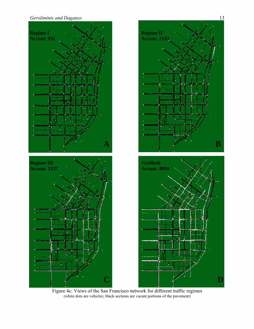
where a(t) is a step function changing with time every 15 minutes. For validating the insensitivity of the proposed macroscopic relations, many different runs were made with different a(t) functions and qij flows. Queueing diagrams with cumulative input-output curves where constructed. By considering the network as a single reservoir system output was estimated using equation 3. We tested the dynamic model predictions under different traffic conditions. Figures 4 and 5 show the most important results of the simulations. First, figure 4a shows travel production-accumulation pairs aggregated per 2 cycles for the whole network for different runs. Four different states of the system (A, B, C and D) have been highlighted for comparison purposes. Figure 4b shows output vs. travel production pairs. We see that unobservable output and observable production are highly correlated for a variety of traffic conditions. Figure 4c shows views of the network during simulation. The four snapshots correspond to the states of figure 4a. State A belongs to regime I when the system is undersaturated and the average speed is about 25km/hr. As demand increases system moves to state B where the vehicle – miles traveled is near the maximum and the average speed is 17km/hr. In state C congestion is broad, long queues are observed and the average speed drops to 7km/hr.


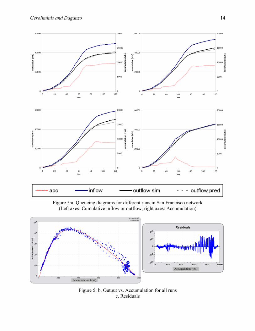
In state D output is near to zero and the majority of vehicles are stopped. We found that when traffic conditions are very near to gridlock (point D) it is very difficult for the system to return to better traffic states (B or C) even if the demand decreases significantly. This means that it is necessary to prevent traffic in cities to move to states of very high accumulation and apply control in a preventive form. . Our experiment validates equation 7 for a real network with a hundred signalized intersections. The proposed relationship is robust for different O-D tables, a range of traffic conditions. By comparing figures 2, 3a and 4a we see that large systems observed over long times are predicted more reliably than small systems; “Bigger is better”. This suggests that large scale (the nemesis of traditional models) actually works in favor of the aggregate approach and that we can shift the modeling emphasis from microscopic predictions to macroscopic monitoring and control. Figure 5a shows queueing diagrams for different runs. Cumulative output was estimated by considering the system as a single reservoir and applying dynamic equation 3. The exit function G(n) is estimated using data points from all the runs and is shown in figure 5b. Figure 5c shows residuals, the differences between the observed and predicted pairs. It is clear that the model can predict output accurately. The last two curves really fit quite closely and they are almost perfectly superimposed when accumulation values do not belong to the decreasing branch of the diagram (Regime III). Predictions of regime III are more difficult, as expected, because the system is chaotic and not in steady state conditions when congested. But any control strategy should try and avoid states in this regime and monitor the states carefully if they arise. So, this is only a minor problem. A question that arises from the above is whether cities experience congestion with production-accumulation pairs in regime III, with speeds considerably less than 50% of the average speed during the off-peak. The answer is yes. The Hellenic Institute of Transportation Engineers reports that during year 2005 average speeds in major arterials in the city of Athens during peak hours were three to five times smaller than the off peak average speeds (e.g. Alexandras Avenue – 5km/hr for peak hour, 25km/hr for non peak, Mesogion Avenue – 8km/hr for peak hour, 40km/hr for non peak) (20). In many European cities speeds in the centre are under 10 kilometers per hour at midday and slower during the rush. Developing countries face up similar problems. Drivers in Bangkok spend the equivalent of 44 days a year in gridlock (19). This suggests that the development of control strategies to relieve congestion and increase mobility could have a significant payoff.


0

300000

600000

900000

1200000

1500000

0 2000 4000 6000 8000 10000

accumulation (vhs)

Trav

el P

rodu

ctio

n (v

h-m

eter

s pe

r 2 c

ycle

s)

Figure 4a: Travel Production vs. Accumulation for different runs in San Francisco network

Outlow = (1/1743) * Travel ProductionR2 = 0.97

0

150

300

450

600

750

900

0 300000 600000 900000 1200000 1500000

Travel Production (vh-meters per 2 cycles)

Out

flow

(vhs

per

2 c

ycle

s)

Figure 4b: Outflow vs. Travel production for different runs in San Francisco network

A

B

C

D


Regime I Regime II Accum: 952 Accum: 2143 c

A B Regime III Gridlock Accum: 5337 Accum: 8934

C D

Figure 4c: Views of the San Francisco network for different traffic regimes (white dots are vehicles; black sections are vacant portions of the pavement)


0

20000

40000

60000

0 20 40 60 80 100 120time

cum

ulat

ive

(vhs

)

0

5000

10000

15000

20000

accu

mul

atio

n (v

hs)

0

20000

40000

60000

0 20 40 60 80 100 120time

cum

ulat

ive

(vhs

)

0

5000

10000

15000

20000

accu

mul

atio

n (v

hs)

Residuals

0 2000 4000 6000 8000 10000-200

-100

0

100

200

0

20000

40000

60000

0 20 40 60 80 100 120time

cum

ulat

ive

(vhs

)

0

5000

10000

15000

20000

accu

mul

atio

n (v

hs)

0

20000

40000

60000

0 20 40 60 80 100 120time

cum

ulat

ive

(vhs

)

0

5000

10000

15000

20000

accu

mul

atio

n (v

hs)

Figure 5:a. Queueing diagrams for different runs in San Francisco network

(Left axes: Cumulative inflow or outflow, right axes: Accumulation)

S = 44.53707465r = 0.98608386

accumulation(vhs)

Out

flow

(vhs

per

2 c

ycle

s)

0 2000 4000 6000 8000 100000

200

400

600

800

1000

Figure 5: b. Output vs. Accumulation for all runs c. Residuals

Accumulation (vhs)

Accumulation (vhs)


DYNAMICS AND CONTROL OF TWO RESERVOIR SYSTEMS Reference (4) derived an ordinary differential equation for the system dynamics of a “one neighborhood (reservoir)” city. One can model a city as a single or multi-reservoir system depending on the geometry, the demand patterns and the distribution of trip destinations among the city. The requirement for homogeneity in traffic loads should determine the number of required reservoirs. Consider now a city partitioned in two reservoirs, R1 internal and R2 external. This could be a case of a city where the internal reservoir R1 attracts most of the trips during the morning commute and the external reservoir R2 generates most of the trips at the same time period. It is assumed that there exists for each of the reservoirs an exit function Gi(ni) (i=1, 2), which describes the steady-state behavior of the system. This function expresses the outflow from reservoir i, as a function of its total accumulation ni. It is also assumed that there exists an entrance function Ci(ni) , which describes the maximum inflow (inflow capacity from now on) to the reservoir Ri from the boundary as a function of its accumulation ni. The causality of function Ci(ni) is that sufficiently large accumulations invariably restrict the input. If the inputs change slowly with time we claim that the system will be near equilibrium all the time, and functions Gi and Ci will also, describe the system in the dynamic case. The outflow from reservoir i has two components; trips finishing inside reservoir i and trips exiting from the reservoir i to finish at reservoir i΄=3-i. We assume that these outflows at time t are analogous to the number of vehicles willing to finish their trip at reservoir i or i΄ and being at reservoir i at time t. If ( )in t is the number of vehicles moving at reservoir i at time t; ( )ijn t is the number of

vehicles moving at reservoir i at time t whose destination is reservoir j; ( )ijq t is the flow

generated at reservoir i with destination reservoir j at time t and ( )ix t is a control variable of

inflow capacity at reservoir i with ( )0 1ix t≤ ≤ , then the dynamic equations between the state variables of the system (n1, n2, 11n , 22n ), the control variables (x1, x2) and the input (qij) of a system with two reservoirs are (time t is not included in the equations):

( ) ( ) ( )

( ) ( ) ( )

min ,

min , , 1, 2 , 3

i i i iii ii i i i i i

i

i ii iii i i i i i i

i i

dn n nq q x C n G ndt n

n n nx C n G n G n i i in n

′ ′ ′′ ′ ′

′

′ ′ ′

⎛ ⎞−= + + ⋅ ⋅ −⎜ ⎟

⎝ ⎠⎛ ⎞− ′− ⋅ ⋅ − = = −⎜ ⎟⎝ ⎠

(10)

( ) ( ) ( )min , , 1, 2 , 3ii i i i iiii i i i i i i i

i i

dn n n nq x C n G n G n i i idt n n

′ ′ ′′ ′

′

⎛ ⎞− ′= + ⋅ ⋅ − = = −⎜ ⎟⎝ ⎠

(11)

Equation 10 describes the conservation of flows for each of the reservoirs. The second term of the right hand side of equation 10 represents the exiting flow from reservoir i to i′ , while the third term the entering flow from reservoir i′ . The last term is the rate vehicles reach their


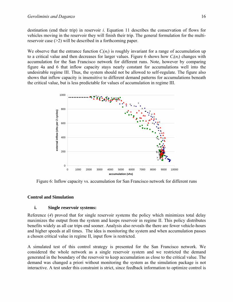
destination (end their trip) in reservoir i. Equation 11 describes the conservation of flows for vehicles moving in the reservoir they will finish their trip. The general formulation for the multi-reservoir case (>2) will be described in a forthcoming paper. We observe that the entrance function Ci(ni) is roughly invariant for a range of accumulation up to a critical value and then decreases for larger values. Figure 6 shows how Ci(ni) changes with accumulation for the San Francisco network for different runs. Note, however by comparing figure 4a and 6 that inflow capacity stays nearly constant for accumulations well into the undesirable regime III. Thus, the system should not be allowed to self-regulate. The figure also shows that inflow capacity is insensitive to different demand patterns for accumulations beneath the critical value, but is less predictable for values of accumulation in regime III.

0

200

400

600

800

1000

0 1000 2000 3000 4000 5000 6000 7000 8000 9000 10000

accumulation (vhs)

exte

rnal

inflo

w (v

hs p

er 2

cyc

les)

Figure 6: Inflow capacity vs. accumulation for San Francisco network for different runs

Control and Simulation

i. Single reservoir systems: Reference (4) proved that for single reservoir systems the policy which minimizes total delay maximizes the output from the system and keeps reservoir in regime II. This policy distributes benefits widely as all car trips end sooner. Analysis also reveals the there are fewer vehicle-hours and higher speeds at all times. The idea is monitoring the system and when accumulation passes a chosen critical value in regime II, input flow is restricted. A simulated test of this control strategy is presented for the San Francisco network. We considered the whole network as a single reservoir system and we restricted the demand generated in the boundary of the reservoir to keep accumulation as close to the critical value. The demand was changed a priori without monitoring the system as the simulation package is not interactive. A test under this constraint is strict, since feedback information to optimize control is


0

10000

20000

30000

40000

50000

60000

70000

0 20 40 60 80 100 120

time

cum

. out

flow

(vhs

)

0

2000

4000

6000

8000

10000

accu

mul

atio

n (v

hs)

outflow with control outflow with no controlaccum with control accum with no control

not possible. The cumulative demand with control was lower than the one without control for every time t. Figure 7 shows that by trying to keep the accumulation in regime II the total outflow of the system increased by 34% (60347 trips instead of 45083 in a 4 hour period).

1 2 3 4

1

4

2 3

Figure 7: Outflow and accumulation with time for the San Francisco network with and without control in the boundary (no feedback in control)

ii. Two reservoir systems:

We simulate here a system with two concentric reservoirs during the morning commute where the majority of people are moving to the centre of a city. We assume that the dynamic behavior of the system is governed by equations 10 and 11.

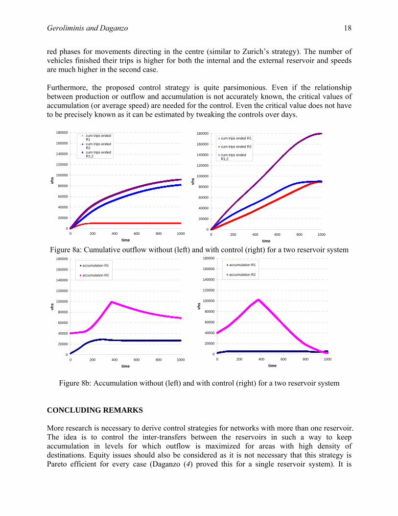
The internal reservoir is ten times smaller than the external reservoir. Vehicles are uniformly distributed in the city and at time zero a small number of vehicles is moving around the city and the rest is parked. Initially, vehicles enter the system at a constant rate; demand decreases with time after 350 time units (total duration of the simulation is 1000 time units). A trip generated from the interval reservoir will finish in the same reservoir with probability f11=0.7, while a trip generated from the external reservoir has equal probability to finish in the internal or the external reservoir (f22=0.5). Similar trapeziums outflow vs. accumulation relationship are assumed for each of the reservoirs. Critical values of the parameters are assumed to be proportional to the size of the reservoirs. First we let the simulation run without applying any control in the boundary of the two reservoirs. We observe (figure 8) that after some time the internal reservoir is subject to gridlock and outflow decreases to zero. We repeat the simulation for the same demand pattern but a simple bang-bang feedback control strategy is applied. When accumulation in reservoir 1 is in regime III, x1=0 and all the other times x1=1. The philosophy of the control is that we try to keep accumulation in the internal reservoir in a range that maximizes outflow. When accumulation is higher than the critical value then inflow capacity in the boundary is restricted. This in practice is feasible by increasing the


0

20000

40000

60000

80000

100000

120000

140000

160000

180000

0 200 400 600 800 1000

time

vhs

accumulation R1

accumulation R2

red phases for movements directing in the centre (similar to Zurich’s strategy). The number of vehicles finished their trips is higher for both the internal and the external reservoir and speeds are much higher in the second case. Furthermore, the proposed control strategy is quite parsimonious. Even if the relationship between production or outflow and accumulation is not accurately known, the critical values of accumulation (or average speed) are needed for the control. Even the critical value does not have to be precisely known as it can be estimated by tweaking the controls over days.

0

20000

40000

60000

80000

100000

120000

140000

160000

180000

0 200 400 600 800 1000

time

vhs

cum trips endedR1cum trips endedR2cum trips endedR1,2

Figure 8a: Cumulative outflow without (left) and with control (right) for a two reservoir system

Figure 8b: Accumulation without (left) and with control (right) for a two reservoir system CONCLUDING REMARKS More research is necessary to derive control strategies for networks with more than one reservoir. The idea is to control the inter-transfers between the reservoirs in such a way to keep accumulation in levels for which outflow is maximized for areas with high density of destinations. Equity issues should also be considered as it is not necessary that this strategy is Pareto efficient for every case (Daganzo (4) proved this for a single reservoir system). It is

0

20000

40000

60000

80000

100000

120000

140000

160000

180000

0 200 400 600 800 1000

time

vhs

cum trips ended R1

cum trips ended R2

cum trips endedR1,2

0

20000

40000

60000

80000

100000

120000

140000

160000

180000

0 200 400 600 800 1000

time

vhs

accumulation R1

accumulation R2


possible that this control favors people live in the centre of a city to people in the periphery. Thus, more opportunities should be given for these people, which usually belong to the poorer community groups. These opportunities could include attractable alternative modes of transport, congestion pricing for vehicles, bus lanes etc. Also, more research is required to develop methodologies for partitioning a city in neighborhoods (reservoirs) for which output and production are governed by equation 5. ACKNOWLEDGEMENTS This material is based upon work supported by a grant from the Volvo Center of Excellence at University of California at Berkeley. We thank professor Alexander Skabardonis for providing the simulated networks. REFERENCES [1] Texas Transportation Institute, (2005), 2005 Urban Mobility Study. (http://mobility.tamu.edu/ums/) Accessed August 12, 2005. [2] FHWA, (2004), Traffic Congestion and Reliability: Linking Solutions to Problems, 2004 FWHA Report prepared by Cambridge Systematics, Inc. with Texas Transportation Institute (http://ops.fhwa.dot.gov/congestion_report/) Accessed July 17, 2005. [3] Small, K., (2004) Urban Transportation. Concise Encyclopedia of Economics, 2nd edition. (Indianapolis: Liberty Fund) [4] Daganzo, C.F., (2006), Urban gridlock: macroscopic modeling and mitigation approaches, Transportation Research part B (on press) [5] Daganzo, C. F., (1998), Queue spillovers in transportation networks with a route choice, Transportation Science 32 (1), 3–11. [6] Joos, Ernst. Deputy Director of Zurich Transport Authority, (2000),Economy and ecology are no contradictions, EcoPlan International. Paris, FR. (http://www.ecoplan.org/politics/general/zurich.htm) Accessed July 14, 2005. [7] Transport for London, (2004), Congestion Charging: Impacts Monitoring, Second Annual Report, London (www.tfl.gov.uk/tfl/cclondon/cc_monitoring-2nd-report.shtml) Accessed August 14, 2005. [8] Wardrop, J. G. (1952). Some Theoretical Aspects of Road Traffic Research. Proceedings of the Institution of Civil Engineers, Vol. 1, Part 2.


[9] Smeed, R. J. (1968). Traffic Studies and Urban Congestion. Journal of Transport Economics and Policy, Vol. 2, No. 1. [10] Smeed, R. J. (1966). Road Capacity of City Centers. Traffic Engineering and Control, Vol. 8, No. 7. [11] Thomson, J. M. (1967). Speeds and Flows of Traffic in Central London: 1. Sunday Traffic Survey. Traffic Engineering and Control, Vol. 8, No. 11. [12] Wardrop, J. G. (1968). Journey Speed and Flow in Central Urban Areas. Traffic Engineering and Control, Vol. 9, No. 11. [13] Zahavi, Y. (1972). Traffic Performance Evaluation of Road Networks by the α-Relationship. Traffic Engineering and Control, Vol. 14, No. 5. [14] Herman, R., Prigogine, I., (1979), A two-fluid approach to town traffic. Science 204, 148–151. [15] Herman, R. and S. A. Ardekani, (1984), Characterizing Traffic Conditions in Urban Areas. Transportation Science, Vol. 18, No. 2. [16] Herman, R., Malakhoff, L., Ardekani, S., 1988. Trip time-stop time studies of extreme driver behaviors. Transportation research. Part A, Vol. 22A, no. 6, 427-433 [17] Williams, J. C., H. S. Mahmassani, and R. Herman, (1987), Urban Traffic Network Flow Models, Transportation Research Record 1112, Transportation Research Board. [18] Mahmassani, H., Williams, J. C., Herman, R., (1987). Performance of urban traffic networks. In: Gartner, N. H., Wilson, N. H. M. (Eds.), 10th Int. Symp. on Transportation and Traffic Theory. Elsevier, Amsterdam, The Netherlands. [19] Edie, L.C. (1963), Discussion of traffic stream measurements and definitions, Proc. 2nd Int. Symp. On the Theory of Traffic Flow, (J. Almond, editor), pp. 139-154, OECD, Paris, France. [20] Federal Highway Administration (2003). CORSIM Version 5.1 Users Manual. US Department of Transportation, Washington DC. [21] Ressler, N. (1999). MIT conference on "Traffic Congestion: A Global Perspective." , 8-9 June, MIT (http://web.mit.edu/newsoffice/1999/traffic-0714.html) Accessed July 20, 2006. [22] Hellenic Institute of Transportation Engineers, (http://www.ses.gr) Accessed April 23, 2006

Documents

Macroscopic modeling of traffic in cities final · Macroscopic modeling of traffic in cities By Nikolas Geroliminis* Institute of Transportation Studies University of California,