Embed Size (px)
Citation preview
This paper presents preliminary findings and is being distributed to economists
and other interested readers solely to stimulate discussion and elicit comments.
The views expressed in this paper are those of the authors and do not necessarily
reflect the position of the Federal Reserve Bank of New York or the Federal
Reserve System. Any errors or omissions are the responsibility of the authors.
Federal Reserve Bank of New York
Staff Reports
Macroprudential Policy:
Case Study from a Tabletop Exercise
Tobias Adrian
Patrick de Fontnouvelle
Emily Yang
Andrei Zlate
Staff Report No. 742
September 2015
Revised December 2015

Macroprudential Policy: Case Study from a Tabletop Exercise
Tobias Adrian, Patrick de Fontnouvelle, Emily Yang, and Andrei Zlate
Federal Reserve Bank of New York Staff Reports, no. 742
September 2015; revised December 2015
JEL classification: G18, E58, G01
Abstract
Since the global financial crisis of 2007-09, policymakers and academics around the world have
advocated the use of prudential tools for macroprudential purposes. This paper presents a
macroprudential tabletop exercise that aimed at confronting Federal Reserve Bank presidents
with a plausible, albeit hypothetical, macro-financial scenario that would lend itself to
macroprudential considerations. In the tabletop exercise, the primary macroprudential objective
was to reduce the likelihood and severity of possible future financial disruptions associated with
the hypothetical overheating scenario. The scenario provided a path for key macroeconomic and
financial variables, which were assumed to be observed through 2016:Q4, as well as the
corresponding hypothetical projections for the interval from 2017:Q1 to 2018:Q4. Prudential
tools under consideration included capital-based tools such as leverage ratios, countercyclical
capital buffers, and sectoral capital requirements; liquidity-based tools such as liquidity coverage
and net stable funding ratios; credit-based tools such as caps on loan-to-value ratios and margins;
capital and liquidity stress testing; and supervisory guidance and moral suasion. In addition,
participants were asked to consider using monetary policy tools for financial stability purposes.
Under the hypothetical scenario, participants found many prudential tools less attractive owing to
implementation lags and limited scope of application and favored those deemed to pose fewer
implementation challenges, such as stress testing, margins on repo funding, and guidance. Also,
monetary policy came more quickly to the fore as a financial stability tool than might have been
thought before the exercise. The tabletop exercise abstracted from governance issues within the
Federal Reserve System, focusing instead on economic mechanisms of alternative tools.
Key words: financial stability, macroprudential policy, monetary policy, financial overheating,
tabletop exercise
_________________
Adrian, Yang: Federal Reserve Bank of New York (e-mail: [email protected],
[email protected]). de Fontnouvelle, Zlate: Federal Reserve Bank of Boston (e-mail:
[email protected], [email protected]). This paper documents a
macroprudential tabletop exercise that was conducted by the members of the Financial Stability
Subcommittee of the Conference of Presidents of the Federal Reserve in June 2015 based on a
hypothetical macro-financial scenario. Additional contributors to preparing the exercise include
Christine Docherty, Joseph Haubrich, Michael Holscher, Charles Morris, Matthew Pritsker, and
Katherine Tilghman Hill. Helpful feedback was provided by Dianne Dobbeck, Rochelle Edge, Ron
Feldman, Nellie Liang, Scott Nagel, Michael Palumbo, Michael Kiley, Fabio Natalucci, Andreas
Lehnert, Kevin Stiroh, Philip Weed, and the subcommittee members William Dudley, Esther
George, Loretta Mester, Narayana Kocherlakota, and Eric Rosengren. The views expressed in this
paper are those of the authors and do not necessarily represent the views of the Federal Reserve
Banks of Boston or New York, or the Federal Reserve System.
1
Table of Contents
Introduction ................................................................................................................................................... 3
1. The Hypothetical Scenario .................................................................................................................... 6
A) Hypothetical Macroeconomic Context ......................................................................................... 6
B) Hypothetical Valuation Pressures ................................................................................................. 7
C) Hypothetical Evolution of Leverage ............................................................................................. 8
D) Hypothetical Liquidity and Maturity Transformation .................................................................. 8
E) Hypothetical Vulnerabilities ......................................................................................................... 9
2. Prudential Tools to Address Risks to Financial Stability .................................................................... 10
A) Capital Regulation ...................................................................................................................... 11
1. Leverage ratios ............................................................................................................................ 11
2. Countercyclical capital buffer (CCyB) ....................................................................................... 12
3. Sectoral risk weights ................................................................................................................... 13
B) Liquidity Regulation ................................................................................................................... 14
1. Liquidity Coverage Ratio (LCR) ................................................................................................ 14
2. Net Stable Funding Ratio (NSFR) .............................................................................................. 15
C) Credit-related tools ..................................................................................................................... 15
1. Caps on loan-to-value (LTV) ratios ............................................................................................ 15
2. Margin requirements for securities financing transactions ......................................................... 16
D) Supervisory Stress tests .............................................................................................................. 17
1. CCAR .......................................................................................................................................... 17
2. CLAR .......................................................................................................................................... 18
E) Supervisory Guidance ................................................................................................................. 19
F) Moral Suasion ............................................................................................................................. 19
3. Monetary Policy Tools to Address Financial Stability Risks ............................................................. 20
A) Permanent Open Market Operations .......................................................................................... 20
B) Forward Guidance ...................................................................................................................... 22
C) Required Reserves ...................................................................................................................... 22
D) Discount Window Lending ......................................................................................................... 22
E) Temporary Open Market Operations .......................................................................................... 23
2
4. Transmission Channels of Macroprudential and Monetary Policies .................................................. 23
A) Transmission Mechanisms for Capital-based Macroprudential Instruments .............................. 23
B) Transmission Mechanisms for Macroprudential Capital Stress Tests ........................................ 24
C) Transmission Mechanisms for Liquidity-based Macroprudential Instruments .......................... 25
D) Transmission Mechanisms for Credit-Related Macroprudential Instruments ............................ 25
E) Transmission Mechanisms of Monetary Policy.......................................................................... 26
5. Summary of the Tabletop Exercise ..................................................................................................... 28
A) Risks to Financial Stability ......................................................................................................... 28
B) Potential Actions to Address Risks to Financial Stability .......................................................... 28
Conclusion .................................................................................................................................................. 30
References ................................................................................................................................................... 31
Figures ........................................................................................................................................................ 33
Tables .......................................................................................................................................................... 38
3
Introduction Since the global financial crisis of 2007-09, policy makers around the world have advocated the
use of macroprudential policy tools for financial stability purposes (Bernanke (2008), Bank of
England (2009), Basel Committee on Banking Supervision (2010), Tarullo (2013)). Academic
work on the implementation of a macroprudential approach has flourished recently (see
Brunnermeier, Markus, Andrew Crockett, Charles Goodhart, Avinash Persaud, and Hyun Song
Shin (2009), Hanson, Kashyap, Stein (2011), and Hirtle, Stiroh, Schuermann (2009)). Even prior
to the crisis, some academics and policy makers argued for a macroprudential approach to
financial regulation (see classic contributions by Robinson (1950) and Bach (1949), and more
recent work by Crockett (2000) and Borio (2003)).
This paper presents a macroprudential tabletop exercise that was conducted by members of the
Financial Stability Subcommittee of the Conference of Presidents (COP) of the Federal Reserve
Banks in June 2015.2 The tabletop exercise was aimed at confronting Federal Reserve Bank
presidents with a plausible, albeit hypothetical, macro-financial scenario that would lend itself to
macroprudential considerations. Before describing the hypothetical scenario, the available policy
tools, and their transmission mechanism in detail, we propose a set of macroprudential objectives
and a framework for use in assessing financial vulnerabilities. Finally, we also describe the
financial stability concerns and actions suggested by the COP members in the context of the
hypothetical scenario.
In the tabletop exercise, the primary macroprudential objective is to reduce the occurrence and
severity of major financial crises and the possible adverse effects on employment and price
stability. The macroprudential objective, because it focuses on economy-wide financial stability,
differs from the Federal Reserve’s monetary policy objectives of full employment and stable
prices and goes beyond its micro-prudential objective of ensuring the safety and soundness of
individual firms. However, the objectives and transmission mechanisms of microprudential,
macroprudential, and monetary policies are intertwined, generating the potential for tradeoffs
among objectives. For example, trade-offs may arise between preemptive macroprudential actions
and the cost of financial intermediation, as preemptive macroprudential actions that reduce
vulnerabilities may slow economic performance in the short term.3 Furthermore, the tradeoff
between macroprudential and microprudential objectives might be more severe in busts than in
booms, while the tradeoff between macroprudential and monetary policy objectives might be more
severe in booms than in busts. Therefore, a secondary objective is to manage such trade-offs, i.e.,
by aiming to mitigate the side effects of macroprudential policy actions through time. Financial
system disruptions that macroprudential objectives aim to avoid include fire sales in financial
markets, destabilizing runs on banking and quasi-banking institutions, shortages of money-like
assets, disruptions in credit availability to the non-financial business sector, spikes in risk premia,
2 The Subcommittee is chaired by Eric Rosengren (Boston) and includes William Dudley (New York),
Esther George (St. Louis), Loretta Mester (Cleveland), and Narayana Kocherlakota (Minnesota). 3 In the longer term, financial stability and economic growth likely complement each other (Dudley, 2011).
4
disorderly dissolution of systemically important financial institutions, excessive spillovers from
disruptions in international funding and currency markets, and disruptions of the payments system.
Our assessment framework of financial vulnerabilities follows Adrian, Covitz, and Liang (2013).
The framework is a forward-looking monitoring program designed to identify and track the
sources of systemic risk over time, and to facilitate the development of policies to promote
financial stability. Under this framework, macroprudential tools/actions can be classified
according to whether they serve preemptive or resilience goals. The preemptive goal (i.e., to
reduce the occurrence of crises) leans against the financial cycle by limiting the build-up of
financial risks to reduce the probability or magnitude of a financial bust. The resilience goal (i.e.,
to reduce the severity of crises) strengthens the resilience of the financial system to economic
downturns and other adverse aggregate shocks. The framework also distinguishes between shocks,
which are difficult to prevent, and vulnerabilities that amplify shocks. Such vulnerabilities may
arise from excessive increases in asset valuations, leverage, and liquidity and maturity
transformation. Nonetheless, the framework monitors vulnerabilities across four sectors of the
economy: the non-financial business sector, the household sector, the banking sector, and the non-
bank financial sector.
The hypothetical scenario provides a path for key macroeconomic and financial variables, which
are assumed to be observed through 2016:Q4, as well as the corresponding projections for the
interval from 2017:Q1 to 2018:Q4, which are assumed to reflect staff forecast and market
expectations as of 2016:Q4. The variables are grouped according to their potential to have a
significant impact on three types of vulnerabilities (valuation, leverage, and liquidity and maturity
transformation) across the four economic sectors noted above (non-financial firms, households,
banks, and non-bank financial institutions). The assessment of financial vulnerabilities by
participants is assumed to take place as of 2017:Q1.
The hypothetical scenario features a compression of U.S. term and risk premia through 2016:Q4—
projected to continue thereafter—which keeps financial conditions loose and fuels valuation
pressures in U.S. financial markets. The compression of risk premia encourages the issuance of
corporate debt and leveraged loans, which boosts leverage in the non-financial business sector.
Also, the real price index in the commercial property market rises rapidly. At the same time, the
non-bank financial sector, including money market mutual funds, expands in size and provides
short-term wholesale funding to the non-financial business sector. These developments occur
while the Federal Reserve removes the degree of monetary accommodation only gradually in 2015
and 2016, as inflation is assumed to persist at slightly below its target rate and unemployment to
persist at the hypothetical scenario-specific non-accelerating inflation rate of unemployment
(NAIRU), as discussed in Section 1. As such, the constraint on monetary policy and looser-than-
desired financial conditions boost the rationale for the use of macroprudential tools.
The hypothetical scenario resembles some well-known cases of financial overheating from recent
decades documented in the literature, although with some notable differences. First, it bears
similarity to the case of New England during the mid-1980s, when rapid growth in regional
mortgage lending led to a real estate boom (FDIC, 1997). Second, the scenario resembles the real
5
estate boom in Sweden during 1989-1990, which was fuelled by accommodative fiscal policies,
rapid growth in lending by banks and mortgage companies, and capital inflows (Englund, 1999;
Jaffee, 1994). However, unlike the cases of New England or Sweden, our scenario places greater
emphasis on the increase in non-financial business leverage as opposed to bank leverage. It also
allows a greater role for the non-bank financial sector as a provider of short-term funding (rather
than mortgage loans as in Sweden) and highlights constraints on monetary tightening that can
keep financial conditions relatively loose. Finally, compared to the U.S. financial crisis in 2008-
2009, our hypothetical scenario highlights an increase in leverage at non-financial firms instead of
households and features overheating in commercial property rather than in the residential housing
market.
There are several types of macroprudential tools that participants considered in pursuing
macroprudential objectives under the hypothetical scenario. Capital-based tools include
countercyclical capital buffers and sectoral capital requirements. Liquidity-based tools include
liquidity and net stable funding requirements. Credit-based tools include loan-to-value (LTV) and
debt-to-income (DTI) caps, margin requirements for securities financing transactions, as well as
other restrictions concerning underwriting standards. Stress tests include capital and liquidity
stress tests. Supervisory guidance and moral suasion including speeches and public
announcements were additional tools that participants in the exercise considered. In addition,
participants could also use monetary policy tools for macroprudential objectives. We note that the
tabletop exercise abstracted from governance issues within the Federal Reserve System, focusing
instead on economic mechanisms of alternative tools.
From among the various tools considered, tabletop participants found many of the prudential tools
less attractive due to implementation lags and limited scope of application. Among the prudential
tools, participants favored those deemed to pose fewer implementation challenges, in particular
stress testing, margins on repo funding, and supervisory guidance. Nonetheless, monetary policy
came more quickly to the fore as a financial stability tool than might have been thought before the
exercise.
The remainder of this paper is structured in five sections. Section 1 describes the hypothetical
macro-financial scenario. Section 2 provides an overview of prudential and monetary instruments
that are available to the Federal Reserve Board and the Federal Open Market Committee
respectively to achieve macroprudential objectives. Section 3 gives a brief description of the
transmission channels of the tools. Section 4 presents a summary of the tabletop exercise that the
Subcommittee for Financial Stability of the Conference of Presidents undertook in June 2015.
Section 5 concludes.

6
1. The Hypothetical Scenario
The scenario assumes that data is observed through 2016:Q4, with 2017:Q1 through 2018:Q4
reflecting staff forecasts and market expectations as of 2016:Q4.4 The scenario features rapid
expansion in U.S. economic activity and gradual removal of monetary accommodation in 2015
and 2016. In this context, a persistent decline in foreign sovereign bond yields and high risk
appetite among investors put downward pressure on the U.S. term and risk premia, which keeps
financial conditions loose and fuels valuation pressures in U.S. markets. Most notably, valuation
pressures emerge in the corporate debt and commercial property markets. The compression of risk
premia encourages the issuance of corporate debt and leveraged loans, which boosts leverage in
the non-financial business sector. The non-bank financial sector expands and provides short-term
wholesale funding to the non-financial business sector. Table 1 provides a summary of indicators
used to monitor three types of risks in the hypothetical scenario (valuation pressures, excess
leverage, and excess liquidity and maturity transformation) across four sectors in the U.S.
economy (non-financial businesses, households, banks, and non-bank financial institutions). The
table also includes a color-coded assessment of the severity of risks in the hypothetical scenario
provided to participants ahead of the Tabletop exercise.
A) Hypothetical Macroeconomic Context
In the United States, it is assumed that there is a sustained, rapid expansion in real economic
activity, which is fueled in part by the overheating of financial markets. Real GDP grows at
3¼ percent per year (Figure 1), unemployment steadily declines to 5 percent by the end of 2016,
while inflation does not exceed 2 percent per year (Figure 2). Beyond 2016, real GDP is forecast
to continue rising at a rate of 3¼ percent per year, unemployment to persist at 5 percent, and
inflation to remain at only 2 percent per year. Despite the rapid pace of GDP growth, U.S.
inflation is dampened by dollar appreciation and stable energy prices amid slow growth in foreign
economies (Figure 1), forces which are expected to persist through 2018. Also, we assume for the
purposes of this scenario that NAIRU is around 5 percent, and that unemployment does not
decline below that level due to fast productivity growth and rising labor force participation.
In the hypothetical scenario, given the decline in unemployment and pick-up in inflation, the
FOMC is assumed to start raising the federal funds target rate in 2015:Q2 and to increase it to
about 1½ percent by the end of 2016 (Figure 3). However, despite rapid GDP growth, the pace of
U.S. monetary tightening is assumed to be constrained by unemployment persisting at 5 percent
and inflation remaining stable at 2 percent over the forecast horizon. Markets expect the federal
funds target rate to rise to only 3 percent by the end of 2018.
4 Without loss of generality, the variables in the hypothetical scenario, which are assumed to be observed
through 2016:Q4, do not exhibit the volatility that characterizes actual macroeconomic and financial time
series data beyond the last data point available at the time when the scenario was built (i.e., 2015:Q1 or
2014:Q4 for most variables). The last actual data point was 2015:Q1 for Figures 1-7 (except for
commercial property prices); 2014:Q4 for Figure 7 (commercial property prices), as well as for Figures 9-
11 and 13-20; 2014:Q3 for Figure 8; and 2013 for Figure 12 (which uses annual data).
7
Downside risks to the hypothetical macroeconomic forecast are due to the potential of adverse
financial developments, especially in markets where overheating concerns persist. Three key risks
are highlighted in the scenario: (1) a severe disruption in the corporate debt market; (2) a sharp
reversal in commercial property prices; and (3) a sudden stop in short-term funding, as discussed
in Sections 1B-1E below. The realization of any of these risks would undermine GDP growth, put
downward pressure on inflation, and increase unemployment.5 In such a case, the relatively low
level of the federal funds rate would curtail the Federal Reserve’s ability to provide monetary
accommodation, and the zero lower bound might again become a binding constraint.
B) Hypothetical Valuation Pressures
Valuation pressures arise in selected U.S. financial markets, fueled in part by spillovers from the
foreign sector and high risk appetite among investors. In particular, sovereign bond yields in the
euro area decline and persist at low levels through late-2016, and are expected to remain depressed
thereafter (Figure 5). Low foreign yields and high risk appetite trigger portfolio reallocations
towards U.S. assets, including Treasury bonds and risky assets. As a result, term premia and risk
premia in U.S. markets narrow, especially for riskier assets (Figure 4). The compression of term
and risk premia leads to looser-than-desired financial conditions in U.S. markets, despite rising
short-term interest rates, providing a rationale for macroprudential policy.
The increased demand for U.S. assets puts upward pressure on U.S. equity prices, dampens stock
market volatility (Figure 6), and compresses the equity risk premium. With the Dow Jones Total
Stock Market index rising 6 percent per year through 2016 (and expected to rise at a similar pace
thereafter), the equity risk premium is expected to narrow by more than one percentage point by
the end of 2018.6
The compression of risk spreads, looser underwriting standards, and rising demand for
commercial mortgage-backed securities (CMBS) fuel growth in commercial mortgage lending. As
a result, valuation pressures emerge in the commercial property market, with the price index
matching its pre-Lehman peak in real terms by end-2016 and expected to exceed it substantially
by end-2018 (Figure 7).
The share of GSE mortgages increases (Figure 8) due to the GSE’s loosened underwriting
standards for prime mortgages and the continued reluctance of banks to engage in nonprime
residential mortgage lending. However, in the aggregate, residential mortgage lending increases
5 A financial bust would impair real economic activity through the same channels that are at work during
the financial boom, i.e., the firms’ lost access to funding would curtail investment, increase unemployment,
and decrease wage growth and inflation; a decline in commercial property prices would also depress
construction. 6 With real GDP growing at 3¼ percent per year, inflation persisting at about 2 percent, and the stock
market rising at 6 percent per year, the dividend yield declines from 2 to 1.95 percent between early-2015
and late-2018. As such, and with the 10-year Treasury yield rising from about 2 percent to 3.15 percent, the
equity risk premium is compressed from 3.33 percent to 2.1 percent during the same interval.

8
more slowly than commercial lending, and hence residential property prices rise more slowly than
commercial prices, remaining below their pre-Lehman peak (Figure 7).7
C) Hypothetical Evolution of Leverage
Leverage in the non-financial business sector rises substantially by late-2016 and is projected to
increase well above its trend by late-2018, measured as either the debt-to-GDP (Figure 9) or debt-
to-assets ratio (Figure 10). The increase in leverage reflects the issuance of corporate bonds and
leveraged loans, especially for riskier firms, which are facilitated by an environment of low risk
premia, high risk appetite, reach for yield, and a continuation of high demand for collateralized
loan obligations (CLOs).
Leverage in the household sector rises more slowly than for non-financial firms (Figures 9 and
10), reflecting the reluctance of BHCs to ease underwriting standards and the relatively slower
growth of residential property lending. Following the fast rise and sharp correction around the
2008 crisis, household leverage remains below its long-term trend as measured by either the debt-
to-GDP or the debt-to-assets ratio.
Banks purchase part of the new corporate debt and issue leveraged loans to non-financial
businesses, increasing their exposure to risk in response to narrower term and credit risk premia.
As regulatory capital requirements are phased in, banks raise more capital and strengthen their
ratios of core capital to assets further (Figure 11). However, there is concern that the ratios of core
capital to risk-weighted assets (not shown) remain flat as banks increase their exposure to risk.
Non-bank financial institutions, such as mutual funds, private equity funds, hedge funds, and
other shadow bank intermediaries, increase their market shares of high-risk corporate debt, CLOs,
ABS, and CMBS. As a result, they grow in size and increase their leverage. As shown in Figure
12, shadow banking liabilities (as a percent of GDP) rise above pre-crisis levels starting in 2016.
D) Hypothetical Liquidity and Maturity Transformation
In the scenario, liquidity ratios improve at large and medium-sized banks (with assets above
$250 billion and $50 billion, respectively) reflecting the phasing in of the Basel III liquidity
coverage ratios (LCR) and net stable funding ratios (NSFR). However, small banks are not
subject to such regulations and increase their exposures to long-term corporate debt and
commercial mortgage loans. As a result, small banks suffer continued deteriorations in the share of
high quality liquid assets (Figure 13) and widening duration gaps between assets and liabilities
(Figure 14).
Money market funds (MMFs) grow in size and increase funding to non-financial firms, banks,
and broker-dealers, leading to an expansion of their size that approaches the pre-crisis peak
7 In our scenario, commercial property prices rise at about 7 percent per year in nominal terms during 2015-
2016, and are projected to continue at the same rate through 2018. Residential property prices rise at a rate
of 4 percent per year during the same interval.
9
(Figure 15). Their maturity and liquidity mismatches continue to raise concern.8 MMF growth is
caused by a reallocation of households and nonfinancial corporations from bank deposits to
MMFs, which pass through rate increases more directly. In turn, MMFs finance non-financial
corporations via commercial paper and finance banks and broker-dealers via repo as well as
securities lending transactions. Repo transactions increasingly use risky corporate debt as
collateral (Figure 16).
As a result, short-term wholesale funding as a fraction of GDP rises from 28 percent in early-
2015 to 35 percent by end-2016, though that is far below the pre-crisis peak of 57 percent (Figure
17). The rise in short-term funding reflects repo, commercial paper, securities lending, and other
forms of money market funding. Short term funding is expected to rise slightly above 40 percent
of GDP by end-2018.
Mutual funds and exchange-traded funds increasingly shift their portfolios away from highly-
liquid Treasuries and Agency debt and toward corporate and sovereign debt, acquiring increasing
shares of the total outstanding in the market (Figure 18). While the risk of fire sales by banks,
broker-dealers, and insurance companies is mitigated due to stricter regulations, the greater size of
mutual funds among corporate bond investors generates new sources of risk.9 Mutual funds are
potentially subject to sudden redemptions that can lower bond liquidity and widen credit spreads,
thus leading to a deterioration of financing conditions for corporate borrowers.
E) Hypothetical Vulnerabilities
Summing up the discussion above, the scenario highlights three key risks in financial markets.
First, one risk is related to the possibility of disruptions in the corporate debt market, such as a
jump in the pricing of credit risk that could result from a sudden reversal in risk appetite or foreign
capital flows, a corporate default cycle, or market overreaction to U.S. monetary policy
normalization.
Second, to the extent that these shocks hit the commercial mortgage market, they amplify the risk
of a sharp correction in commercial property prices. Disruptions to the corporate debt and
commercial mortgage markets would affect the real economy both directly, as non-financial firms
lose access to financing and reduce their investment, but also indirectly, as lenders suffer valuation
8 Despite the compliance date of October 2016 for new reforms, concerns about the MMMFs’ maturity and
liquidity mismatches persist, since the floating NAV in itself may not entirely eliminate the risk of investor
runs, and the prime retail funds are still exempt from the floating NAV. 9 The Investment Company Act of 1940, enforced by the SEC, requires that open-ended mutual funds not
hold more than 15 percent of net assets in illiquid securities. Although the rule aims to limit the mutual
funds’ holdings of illiquid corporate debt, in practice the SEC defines “illiquid securities” only broadly,
i.e., as securities that “may not be sold or disposed of in the ordinary course of business within seven days
at approximately the value at which the mutual fund has valued the investment on its books.”

10
losses and cut lending further. The cost to the real economy increases with the size of markets
affected and the range of institutions involved (see Figures 19 and 20).10
Third, the increased reliance on short-term wholesale funding leaves banks and non-bank financial
intermediaries vulnerable to the risk of runs on their short-term liabilities. In particular, as repo
funding increasingly uses risky corporate bonds as collateral (Figure 16), disruptions in the long-
term corporate bond market would impair short-term funding. Consequently, given the increasing
extent of maturity transformation at financial intermediaries, disruptions in short-term funding
would have additional negative consequences on the long-term debt markets as well. In particular,
due to increased concentration in illiquid corporate debt, hedge funds and bond mutual funds
become increasingly vulnerable to large redemptions in the event of adverse shocks to the
corporate bond market, which would cause fire sales and exacerbate the downward pressure on
asset prices.
2. Prudential Tools to Address Risks to Financial Stability
This section outlines the range of regulatory and supervisory tools that the Board of Governors of
the Federal Reserve System can potentially utilize to mitigate the impact of cyclical variations in
financial stability risks due to overheating or the realization of stress scenarios. The utilization of
some tools will need to be coordinated with other banking regulators.
There are six broad categories of tools: (1) capital regulation; (2) liquidity regulation; (3) credit
regulation; (4) supervisory stress tests; (5) supervisory guidance; and (6) moral suasion. The
purpose of the exercise is for Committee members to gain a better understanding of the
practicalities involved in applying macroprudential tools, and is not to opine on which tools would
be applicable in the current economic environment.
We describe each tool, its scope of application, whether it applies to downturn and/or overheating
scenarios, and its associated implementation challenges or limitations. Several broad themes
emerge across the tools considered in the exercise.
o Prudential tools can be used to build resilience against shocks, in addition to leaning against
emerging risks to financial stability.11
This is an advantage over monetary policy, which would
address financial stability concerns only by “leaning against the wind.”
10
By holder, U.S. banks had little exposure to bonds (i.e., held about 6 percent of the total outstanding in
late-2014), the bulk of which was held by U.S. shadow banking institutions, U.S. insurance companies, and
foreign entities (each holding about one quarter of the total outstanding). In contrast, U.S. banks had larger
exposures to commercial mortgages (holding 56 percent of the total), along with ABS issuers, life insurers,
and real estate investment trusts (15, 13, and 8 percent). Finally, U.S. banks and credit unions held the
majority of loans other than mortgages (87 percent of the total). These statistics are based on the Financial
Accounts of the United States, published by the Board of Governors of the Federal Reserve. 11
For example, capital regulation can be used to build resilience, as the capital buffer serves to absorb
unexpected losses at individual firms. To the extent that increased capital requirements discourage lending
activity in the affected sector(s), capital regulation can also be used to “lean against the wind.”
11
o Many (though not all) tools can be used to target specific exposures. This ability to target
exposures is a potential advantage relative to monetary policy tools – to the extent that
policymakers are concerned only about a specific sector.
o Most of the tools are subject to a lag between the time policy makers decide to apply the tool
and the time the tool actually becomes effective. In many instances, this lag may arise from
administrative processes.
o Several tools are more effective in the run up than during crises or recessions.12
This
characteristic proved relevant during the exercise as the scenario considered involves
overheating.
o Many tools are subject to limitations in their scope of application, with most applying only to
banking organizations rather than to the full range of entities engaged in financial
intermediation.
The set of prudential tools together with their limitations is further outlined in Table 2.
A) Capital Regulation
1. Leverage ratios13
The Federal Reserve Board’s minimum leverage ratios require banking organizations to hold at
least a minimum amount of capital relative to their exposures. The U.S. regulatory capital rules
include two leverage ratios: the leverage ratio and the supplementary leverage ratio (SLR).
o The leverage ratio applies to all banking organizations subject to the Federal Reserve
Board’s regulatory capital rules.14
It is measured as tier 1 capital divided by average total
consolidated assets. The minimum leverage ratio requirement is 4%.15
o The SLR is effective January 1, 2018, and will apply only to advanced approaches banking
organizations.16
It will be measured as tier 1 capital divided by total leverage exposure,
which equals the daily average total consolidated assets plus certain off-balance sheet
exposures. The minimum SLR requirement will be 3%.
12
As discussed below, countercyclical capital buffers, loan-to-value ratios, margins, and supervisory
guidance would apply in a downturn only under specific circumstances. 13
See 12 CFR 217.10. 14
It generally does not apply to bank holding companies or savings and loan holding companies with less
than $1bn in total consolidated assets. 15
All insured depository institutions are required to meet a 5% tier 1 leverage ratio requirement to be
considered “well capitalized” under the Prompt Corrective Action (PCA) framework. The PCA framework
is intended to ensure that problems at the insured depository institutions are addressed promptly and at the
least cost to the Depository Insurance Fund. Insured depository institutions that fail to meet the capital
measures under the PCA framework are subject to increasingly strict limits on their activities, including
their ability to make capital distributions, pay management fees, grow their balance sheets, and take other
actions. 16
Advanced approaches banking organizations are those with at least $250bn in total consolidated assets or
at least $10bn in consolidated on-balance sheet foreign exposures.
12
o In addition, effective January 1, 2018, there will be an enhanced SLR requirement
applicable to U.S. top-tier bank holding companies identified as globally systemically
important banking organizations (G-SIBs). The enhanced requirement consists of a 2%
leverage buffer above the minimum SLR requirement for a total of 5%.17
Minimum leverage requirements may be used as a countercyclical tool in downturn or overheating
scenarios in accordance with applicable administrative processes. For example, U.S. banking
agencies issued public notices in times of anticipated unusual and temporary asset growth (e.g.,
influx of deposits that increases average total assets in the lead-up to Y2K and in the period
following the terrorist attacks of September 11th) that acknowledged the potential for declines in
banking organizations’ leverage ratios ).18
In addition, under the enhanced SLR, banking
organizations’ capital levels may fall below the leverage buffer amount without breaching the 3%
regulatory minimum requirements, allowing banking organizations to continue lending activities
during times of stress, albeit subject to restrictions on distributions and discretionary bonus
payments.
Limitations and other considerations
Leverage ratios do not differentiate across exposure types (i.e., the same capital requirement
generally applies to all assets). In addition, as noted above, the SLR standard only applies to a
subset of the largest banking organizations. Moreover, any public notice that acknowledges
temporary asset growth due to exogenous factors that might adversely impact banking
organizations’ minimum leverage ratios would require timely interagency agreement, which
would need to be balanced against concerns that a poorly-timed message might signal run a
potential crisis.
2. Countercyclical capital buffer (CCyB)19
As part of Basel III regulatory reform, banking organizations are required to hold a capital
conservation buffer (CCB) in an amount greater than 2.5% of total RWAs. The CCB is composed
of common equity tier 1 capital, and is in addition to the minimum risk-based capital
requirements. The capital conservation buffer may be expanded, up to additional 2.5% of total
RWAs for a maximum buffer of 5%, for advanced approaches banking organizations as defined
earlier. The additional CCB (above 2.5%) is referred to as the countercyclical capital buffer
(CCyB). The CCyB amount in the U.S. rule is currently 0%.20
When a banking organization does
17
Maintaining an SLR of 5% percent or less results in restrictions on distributions and certain discretionary
bonus payments (though not in the form of a PCA requirement, as BHCs are not subject to PCA
requirements). Insured depository institutions of G-SIBs will be required to meet a 6% SLR in order to be
considered “well capitalized” under the PCA framework. 18
Given that such declines had the potential to result in consequences for the banks under PCA, banking
organizations were encouraged to inform the banking agencies if capital ratios were to fall and to discuss
options to address any temporary breach of capital ratio minimum requirements. 19
See 12 CFR 217.11. 20
Under the reciprocity agreement reached by the United States and other member countries at the Basel
Committee, a U.S. banking organization’s CCyB amount can be affected by the setting of the CCyB in all
jurisdictions where it maintains private sector credit exposures.
13
not maintain its CCB (plus any relevant CCyB), it would be subject to dividend and discretionary
bonus payment restrictions.
The U.S. banking agencies can adjust the buffer from 0% to 2.5% based on a range of
macroeconomic, financial, and supervisory information indicating an increase in systemic risk.21
Increases to the CCyB would be effective 12 months from the date of announcement or earlier if
the agencies articulate the reasons why an earlier effective date is needed. Decreases to the CCyB
would be effective on the day following announcement of the final determination. Unless
extended, the CCyB would return to 0% 12 months after the effective date.
Given that the CCyB could be activated prior to a period of stress, it could require banking
organizations to raise capital when capital is relatively cheap and the system is not under stress. In
addition to its prudential objective of achieving better capitalized banking organizations, this
might further restrain the build-up of financial system vulnerabilities by influencing the amount
and terms of credit conditions. Likewise, the CCyB could allow capital requirements to decrease
in a stress period or enable banking organizations to withstand greater losses than if they did not
have a buffer before their solvency is called into question. Thus, the CCyB can be applied to both
downturn and overheating scenarios, although it can only be applied in downturn scenarios after
the CCyB has been activated.
Limitations and other considerations
The CCyB does not differentiate across exposure types. While it could be activated and de-
activated based on vulnerabilities identified for specific exposures, the CCyB would be applied at
the overall bank level, and not at the targeted exposure level. In addition, there is a 12-month lag
for any increase in the CCyB to become effective (with the possibility of exceptions). Finally,
adjustments to the CCyB will be based on a determination made jointly by the banking agencies.
Because the CCyB amount would be linked to the condition of the overall U.S. financial system
and not the characteristics of an individual banking organization, the banking agencies expect that
the CCyB amount would be the same at the depository institution and BHC level.
3. Sectoral risk weights
Apart from the Basel III-based CCyB, countries such as the United Kingdom, Switzerland, and
Israel have utilized sectoral capital requirements, which apply additional capital requirements on
exposures to specific sectors judged to pose a risk to the system. Sectoral risk weights might also
be used to reduce capital requirements on safer sectors during a downturn.
Limitations and other considerations
Sectoral risk weights could be applied to both downturn and overheating scenarios in accordance
with applicable administrative processes. It could differentiate across exposure types. However,
21
Such information includes the ratio of credit to GDP, a variety of asset prices, other factors indicative of
relative credit and liquidity expansion or contraction, funding spreads, credit condition surveys, indices
based on credit default swap spreads, options implied volatility, and measures of systemic risk.

14
banking organizations may choose to meet the additional capital requirements for the targeted
sector by reducing other exposures in other sectors.
B) Liquidity Regulation
1. Liquidity Coverage Ratio (LCR)22
The Liquidity Coverage Ratio mandates a minimum amount of unencumbered high-quality liquid
assets (i.e., numerator of the ratio) that a banking organization must hold to withstand net cash
outflows over a 30-day stress period (i.e., denominator) characterized by simultaneous
idiosyncratic and market-wide shocks.
Beginning in January 2017,23
banking organizations with assets equal or greater than $250 billion
or with foreign exposure equal or greater than $10 billion must meet a 100% LCR on a daily
basis.24
Banking organizations with assets between $50 billion and $250 billion with foreign
exposure less than $10 billion are subject to a modified LCR, which will be measured monthly.
The U.S. LCR requires banking organizations that are subject to daily compliance and fall below
the minimum threshold for a period of three consecutive business days to promptly submit a
remediation plan to their primary regulator. The rule does not impose a fixed requirement to BHCs
that are subject to monthly U.S. LCR compliance, but rather allows for supervisory discretion
when determining if a remediation plan is necessary. In both cases, the rule does not mandate a
specific timeframe for returning to full compliance. The allowance for supervisory discretion in
determining the timeframe for remediating an LCR shortfall should enable banking organizations
to appropriately utilize their liquidity resources during a period of stress, mitigating the effects of
idiosyncratic and market-wide shocks.
Limitations and other considerations
The LCR could be applied to downturn scenarios, via supervisory discretion, and to overheating
scenarios in accordance with applicable administrative processes. The LCR does not differentiate
exposure types and only applies to a subset of banking organizations as described earlier. Banking
organizations may be reluctant to draw down their their high-quality liquid assets buffer,
particularly in an idiosyncratic stress event that does not immediately affect other market
participants, if the usage of these resources could be perceived as a negative signal. In addition,
there will be need for coordination across U.S. banking agencies in determining the response to an
LCR breach, as well as assessing the appropriate timeframe for returning to compliance.
22
See 12 CFR 249. 23
January 2017 marks the end of the LCR phase-in period, which began in January 2015 for banking
organizations subject to the full LCR, and will begin in January 2016 for banks subject to the modified
LCR. 24
All subsidiaries of these institutions that are insured depositories with assets greater than or equal to $10
billion also are independently subject to the U.S. LCR requirement.

15
2. Net Stable Funding Ratio (NSFR)25
The Net Stable Funding Ratio measures a banking organization’s sources of stable funding
relative to its on- and off-balance sheet exposures, weighted by factors reflective of the exposures’
inherent liquidity characteristics. The Basel III NSFR was finalized in October 2014. The U.S.
regulatory agencies have not yet issued a domestic rule to implement the NSFR.
The Basel NSFR standard does not contain any prescriptive measures regarding enforcement of an
NSFR breach or remediation of a shortfall. If the U.S. agencies implement an approach similar to
the LCR, banking organizations may be able to fall below the NSFR threshold during periods of
stress or credit contraction when market funding is scarcest.
Limitations and other considerations
The NSFR does not differentiate across exposure types. The flexibility of U.S. policymakers to
allow for and respond to temporary NSFR shortfalls will not be known until the U.S. NSFR rule is
finalized; any flexibility likely will require coordination across the banking agencies. In addition,
the NSFR may only apply to a subset of banking organizations, similar to the LCR.
C) Credit-related tools
1. Caps on loan-to-value (LTV) ratios
Credit-related tools are another macroprudential approach being used in countries such as Canada,
Norway, and Korea. These tools include caps on LTV ratios, which restrict credit based on the
value of the underlying collateral and hence dampen demand for a specific lending activity. These
tools can increase the resilience of the banking system by decreasing both the probability of
default and loss given default.26
The U.S. banking agencies have authority to issue rules applicable to insured depository
institutions’ real estate related lending activity. The U.S. banking agencies have issued supervisory
guidance on prudent underwriting practices that includes maximums for LTV ratios that vary by
real estate loan type, derived at the time of loan origination. The Federal Reserve Board could
amend the guidance to increase the LTV standards. In addition, the Federal Reserve Board’s
regulatory capital rules incentivize banks to have prudent underwriting standards by differentiating
capital requirements among exposures based on whether or not they were underwritten in
compliance with the guidance27
. Under the regulatory capital rules, the Federal Reserve Board
could increase the capital that must be held against exposures that were not underwritten in
compliance with the guidance.
25
See http://www.bis.org/bcbs/publ/d295.htm. 26
Credit-related tools also include caps on debt-to-income (DTI) ratios, which are similar in many aspects
to the caps on LTV ratios. The caps on DTI ratios can restrict certain types of loans based on the
borrower’s income. Hence, lower DTI caps can reduce banks’ exposure to certain assets, thus addressing
against overheating concerns in specific sectors and enhancing banks’ resilience to shocks. 27
See 12 CFR 217.32
16
Limitations and other considerations
Lower LTV ratios can be attained during overheating scenarios by tightening the caps. However,
this tool would likely not be effective in downturn scenarios. While the LTV caps could be relaxed
to increase credit demand, banking organizations might steer away from such loans in downturn
scenarios. Therefore, supervisors generally would be relaxing a non-binding constraint. LTV ratio
caps can differentiate exposure types based on the type of collateral.
Use of the tool will only impact a subset of lenders and, therefore, may not substantially affect
lending activity in a particular segment of the U.S. economy as long as banking organizations hold
only a small portion of newly originated mortgages.
2. Margin requirements for securities financing transactions
Setting minimum initial and variation margins for securities financing transactions can constrain
excess leverage in the financial system and dampen demand for the assets being financed. Margin
requirements can vary based on credit conditions; the minimum requirement can be increased in
an overheating scenario to reduce the leverage available to borrowers, and it can be reduced in a
time of stress to lower the pressure on borrowers to post additional margin or face firesale risk.
The Federal Reserve Board has authority under the Securities and Exchange Act of 1934 to set
initial and variation margin requirements for financing collateralized by securities that are
extended by broker-dealers, banks, and other non-bank lenders. Although the Federal Reserve
Board used this tool to adjust the initial margin requirements for the equity markets between 1934
and 1974 to limit excess leverage used by investors, it has not used this tool since then.
The Federal Reserve Board could consider using this authority to set and change the minimum
initial and variation margin requirements for securities financing transactions, such as reverse
repurchase agreements, across the financial system. The minimum margin requirements could be
based on what the Financial Stability Board has recommended, as described in the section below.
However, its authority under the Securities Exchange Act of 1934 to impose minimum margin
requirements for securities finance transactions is limited in certain ways. That statute does not
include authority to impose minimum margin requirements for credit extended on U.S.
government and agency securities by all lenders (whether broker-dealers, banks or non-bank
lenders).
The Financial Stability Board has recently finalized a framework of minimum haircuts on non-
centrally cleared securities financing transactions in which financing against collateral other than
government securities is provided to entities other than banks and broker-dealers.28
In addition,
non-centrally cleared SFTs performed in any operations with central banks are also outside the
scope of application.
Securities financing transactions provided by regulated or unregulated lenders to unregulated
borrowers (e.g., hedge funds) will be within the scope of the FSB framework to limit the build-up
28
http://www.financialstabilityboard.org/wp-content/uploads/SFT_haircuts_framework.pdf.

17
of excessive leverage outside the banking system and maintain a level-playing field between
regulated and unregulated securities financing lenders. Financing provided to banks and broker-
dealers subject to adequate capital and liquidity regulation on a consolidated basis are excluded
because applying numerical haircut floors to those transactions may duplicate existing regulations.
Limitations and other considerations
Margin requirements can be applied to overheating scenarios by raising the minimum margin
requirements. However, this tool would likely not be effective in stress scenarios for the same
reason that the LTV cap would not be effective in such scenarios. They also can differentiate
exposure types based on the type of collateral. However, to be effective, there is a need to have
coordinated responses from other jurisdictions (both introducing the initial margin requirements
and subsequent adjusting). Otherwise, borrowers might circumvent the minimum margin
requirements if they are able to borrow from an overseas market in a manner not subject to the
scope of the margin requirements. The Federal Reserve Board will need to issue a proposed
rulemaking to impose margin requirements.
D) Supervisory Stress tests
1. CCAR29
The Federal Reserve Board’s annual Comprehensive Capital Analysis and Review (CCAR)
applies to bank holding companies with assets of $50 billion or more.30
It includes both a
qualitative review of a banking organization’s capital planning process and a quantitative
assessment of the banking organization’s ability to maintain capital ratios above the required
minima under stressful scenarios. The Federal Reserve Board can object to a bank’s capital plan
and capital distributions for qualitative reasons, quantitative reasons, or both. The scenarios and
outcomes are disclosed to the public.
When identified vulnerabilities rise to prominence in the months before CCAR scenarios are
issued, the Federal Reserve Board could adapt the supervisory scenarios to stress these
vulnerabilities in a timely fashion. If the Federal Reserve Board pre-announced supervisory
scenarios targeting specific exposures before the stress test “as of date” (i.e., before December 31)
and also signaled that those scenarios would be repeated for future CCAR cycles until the
concerns are addressed, then banks (especially those whose capital ratios under the scenario fall
below the required minima) might be incented to adjust their holdings accordingly over time.31
29
See 12. CFR 225.8. 30
In addition, intermediate holding companies of foreign banking organizations will become subject to the
capital plan rule starting in 2017. 31
If the FRB did not signal that the scenarios would be repeated in future CCAR cycles, then the impact
might be limited as banks could understate stress outcomes by temporarily exiting those exposures and
buying them back after the “as of date”.
18
Limitations and other considerations
CCAR could be applied as a macroprudential tool in both downturn and overheating scenarios. It
also can differentiate exposure types based on the design of stressed scenarios. As noted above,
CCAR applies only to a subset of banking organizations and is an annual exercise, making it less
timely than other tools. When identified macro-financial vulnerabilities occur between two annual
CCAR cycles, the Capital Plan Rule, which governs CCAR, allows the Federal Reserve Board to
require a single banking organization, a subset of banking organizations or all banking
organizations to re-submit their capital plans. Resubmission is required if the Federal Reserve
Board determines that changes in financial markets or macro-economic outlook that could have a
material impact on the BHC’s risk profile and financial condition require the use of updated
scenarios.32
In addition, certain vulnerabilities, such as the origination of loans destined to be
sold to non-banks, may be difficult to stress via a macroeconomic or market scenario, requiring a
change to the stress test framework.
2. CLAR
The FRB’s annual supervisory Comprehensive Liquidity Assessment and Review (CLAR)
exercise aims to improve banking organizations’ liquidity resilience by assessing the adequacy of
the firms' liquidity positions in light of each firm’s own risks and evaluating the strength of the
firms' liquidity risk management33
. CLAR involves evaluation of a banking organization’s
liquidity positions through a range of supervisory liquidity analysis such as funding
concentrations, longer funding horizons, and limits on short-term wholesale funding. It also
involves the evaluation of the firms’ own internal stress tests such as the firm’s assumptions
regarding liquidity needs for its prime brokerage services and derivatives trading in stress
scenarios.
The qualitative and quantitative review of stress testing and liquidity management and
measurement practices can influence a banking organization’s internal view of its ability to
withstand shocks, and consequently decision making around taking liquidity risks and reserving
against these risks.
Limitations and other considerations
CLAR could be applied as a macroprudential tool in both downturn and overheating scenarios. It
also can differentiate exposure types based on the scope of supervisory analysis and review.
CLAR is under the sole purview of the Federal Reserve Board.
CLAR applies to a subset of banking organizations that are in the Federal Reserve’s Large
Institution Supervision Coordinating Committee (LISCC) portfolio.34
In addition, although CLAR
32
The FRB could require banks to resubmit capital plans within 30 calendar days of certain events
including changes in financial markets or the macro-economic outlook that could have a material impact on
a bank’s risk profile or financial condition that would require the use of updated scenarios. 33
Per the enhanced prudential requirements of Section 165 of the Dodd Frank Act. 34
See www.federalreserve.gov/bankinforeg/large-institution-supervision.htm for a current list of firms in
the LISCC portfolio.
19
is structured as a continuous monitoring process over the year, supervisory evaluations are
delivered annually, and thus there may be delays between supervisory assessments and reactions
or implementation by banking organizations. Finally, supervisory stress scenarios and outcomes
from CLAR are not currently disclosed to the public as they are deemed “confidential supervisory
information,” and therefore modifications to this supervisory approach may have a limited impact
on market expectations as the market will not know what changes are introduced by the Federal
Reserve Board in a given CLAR.
E) Supervisory Guidance
The Federal Reserve Board and other bank regulators can address potential risks arising from a
particular activity by issuing supervisory guidance. Supervisory guidance can be effective in
establishing expectations for banks and banking organizations related to governance, risk
management and measurement, stress testing, valuation and disclosure. For example, the U.S.
banking agencies issued SR 13-3, “Interagency Guidance on Leveraged Lending,” to address
concerns with deterioration of underwriting practices.35
Limitations and other considerations
Supervisory guidance could be applied to overheating scenarios. It could be applied to downturn
scenarios to the extent supervisors find it appropriate to clarify their expectations. Supervisory
guidance can differentiate across exposure types by targeting a specific activity. The Federal
Reserve Board can issue guidance that applies to BHCs only without interagency coordination but
would need the agreement of the other U.S. banking agencies to issue guidance that is more
broadly applicable. Although issuing guidance can be expeditious compared to a rulemaking,
doing so in coordination with other bank regulatory agencies can still take time.
F) Moral Suasion
Federal Reserve policy makers could appeal to banks to address risks arising from a particular
activity. This approach also can be applied to influence other market participants. Such approaches
could include public speeches or interviews by senior policy makers, discussions with the
executives of supervised banks, and industrywide meetings involving all markets participants. For
example, the FRB played a key role in organizing meetings between the Long-term Capital
Management and a consortium of 14 large bank and non-bank financial institutions that ultimately
resolved the troubled hedge fund in 1998 (see Greenspan 1998).
Limitations and other considerations
This approach can be implemented quickly. In addition, it can be applied to both downturn and
overheating scenarios and can differentiate exposure types by targeting a specific activity. The
FRB can seek to influence non-bank market participants but cannot require them to make changes.
35
SR 13-3 requires a bank that purchases leveraged loans to apply the same standards of prudence, credit
assessment techniques, and in-house limits that would apply if the bank originated the loans; sets
expectation on underwriting and risk management standards for leveraged loans; encourages originating
institutions to be mindful of the reputational risk associated with poorly underwritten leveraged
transactions; and requires the banks to conduct periodic stress testing.
20
3. Monetary Policy Tools to Address Financial Stability Risks
This section outlines the range of monetary policy tools that the Federal Reserve can potentially
use to mitigate the risks to financial stability arising from either the overheating of financial
markets or from the realization of adverse outcomes in the hypothetical scenario.
For the purpose of financial stability objectives in the tabletop exercise, monetary policy tools can
be classified into five broad categories: (1) permanent open market operations (OMOs);
(2) forward guidance; (3) reserve requirements; (4) discount window lending; (5) temporary
OMOs. The tools in each of these categories and their main characteristics are outlined in Table 3.
The remainder of this section presents the tools and discusses their potential to address risks to
financial stability, their applicability during boom vs. bust scenarios, their potential to affect
specific markets and institutions, as well as challenges or limitations in their implementation.
To give a brief summary of the findings below, several broad themes emerge across the monetary
policy tools considered, which highlight both advantages and limitations of deploying monetary
policy tools for financial stability objectives:
o In general, monetary policy tools can lean against risks to financial stability arising from
valuation pressures, excessive leverage, and liquidity and maturity transformation.
o Monetary policy tools benefit from quick implementation once the policy decision is made, in
contrast to macroprudential tools – many of which involve implementation lags.
o Most monetary policy tools apply symmetrically during booms and busts. (The discount
window and emergency lending facilities are exceptions, as they help mostly during busts).
o Monetary policy tools have a broad reach; they can affect financial conditions in both the
banking and the non-banking financial sectors.
o However, monetary policy tools are blunt, as they cannot target specific asset classes, like
many macroprudential tools do (perhaps with the exception of threshold-based forward
guidance).
o Using monetary policy tools to address risks to financial stability could lead to conflicts
between policy objectives, i.e., monetary tightening may reduce the risks of overheating in
specific sectors at the cost of slowing economic growth more broadly.
A) Permanent Open Market Operations
The permanent OMOs consist of outright purchases (or sales) of securities by the Federal Reserve
in pursuit of longer-term goals, such as increasing (or decreasing) the amount of reserves available
to banks. (In contrast, temporary OMOs are driven by short-term factors, such as temporary spikes
in the needs for reserves.) Under Section 14 of the Federal Reserve Act, the Federal Reserve has
the authority to purchase or sell a range of assets that include Treasury securities, agency debt, and
agency mortgage-backed securities (MBS), which result in changes in the size of the Federal

21
Reserve balance sheet and the supply of reserve balances.36
The OMOs follow decisions by the
Federal Open Market Committee (FOMC) and are implemented by the Trading Desk at the
Federal Reserve Bank of New York, which trades with qualified primary dealers.
Depending on the type of securities traded, the permanent OMOs can be divided in a number of
tools and intermediate goals, as follows:
o To bring the federal funds rate in line with the target set by the FOMC (i.e., the interest
rate at which depository institutions trade reserves with each other overnight), the Federal
Reserve purchases (or sells) Treasury securities to inject (or drain) reserves from the market,
and thus to lower (or raise) the federal funds rate.
o To influence longer-term interest rates, the Federal Reserve can also trade longer-term
securities, such as agency debt, agency MBS, and longer-term Treasuries.37
o To influence term premia, the Federal Reserve engages in simultaneous but opposite
transactions with short-term and long-term securities, thus affecting the slope of the yield
curve of the underlying asset.38
Permanent OMOs can serve financial stability goals in a number of ways. For instance, monetary
tightening can curb valuation pressures and excess leverage by limiting credit growth (e.g., either
by restraining credit demand via the interest rate channel, or by reducing credit supply via the
bank lending and bank capital channels, which are discussed below).39
Monetary tightening can
also enhance liquidity by increasing the amount of liquid assets (other than cash) available in the
market as the Federal Reserve sells liquid Treasury securities; and can reduce the incentive for risk
taking by increasing the yields of safe assets. OMOs can be applied immediately, can work during
booms and busts, and can affect financial conditions in sectors where macroprudential tools
generally cannot reach, such as the non-bank financial sector. However, OMOs cannot be
36
Agency debt refers to the debt of government-sponsored enterprises such as Fannie Mae, Freddie Mac,
and Ginnie Mae. Agency MBS refers to MBS guaranteed by the afore-mentioned government-sponsored
enterprises. 37
After the federal funds target rate was effectively reduced to the Zero Lower Bound in late-2008 (i.e., a
target range between zero and 25 basis points), the Fed implemented three Large-Scale Asset Purchase
(LSAP) programs between December 2008 and October 2014, by purchasing longer-term securities
(agency debt, agency MBS, and Treasury securities) with the goal of putting downward pressure on longer-
term interest rates. For a summary of LSAPs, see
http://www.federalreserve.gov/monetarypolicy/bst_openmarketops.htm. While the purchases were
discontinued in October 2014, the Federal Reserve still purchases MBS under a policy in which principal
payments from its holdings of agency debt and agency MBS are reinvested in agency MBS. 38
For instance, under the Maturity Extension Program from late-2011 to end-2012, the Federal Reserve
extended the average maturity of its holdings of Treasury securities in order to decrease longer-term
interest rates, by purchasing securities with remaining maturities of 6 years to 30 years and selling an equal
par amount of securities with remaining maturities of 3 years or less. For MEP, see
http://www.federalreserve.gov/newsevents/press/monetary/20110921a.htm and
http://www.newyorkfed.org/markets/opolicy/operating_policy_110921.html 39
The transmission channels of monetary policy are explained in the next section. Transmission channels
include the interest rate channel, the balance sheet channel, the bank lending channel, the bank capital
channel, and the risk taking channel.

22
deployed for targeted effects on specific sectors (i.e., selling Treasuries tightens financial
conditions throughout the economy, not only in targeted sectors with overheating concerns).
Finally, using OMOs for financial stability may lead to conflicts among policy objectives (e.g.,
they may curb the growth in commercial real estate prices and corporate leverage, but at the cost
of dampening inflation pressures even more and pushing unemployment above the hypothetical
scenario-specific NAIRU).
B) Forward Guidance
With the federal funds rate at the Zero Lower Bound, the Federal Reserve has increasingly used
forward guidance to signal the future path of monetary policy as a way to affect longer-term
interest rates. Since December 2008, the FOMC press releases have included language suggesting
that the federal funds target rate would remain exceptionally low “for some time”, “for an
extended period”, at least until a specific date, or at least as long as unemployment and inflation
do not breach certain thresholds (i.e., threshold-based forward guidance). Announcing that the
federal funds rate would remain low by more than previously anticipated may provide monetary
stimulus by reducing long-run interest rates (see Del Negro, Gianoni, and Patterson, 2015;
Harrison, Korber, and Waldron, 2015; McKay, Nakamura, and Steinsson, 2015).
In principle, a form of threshold-based forward guidance could be deployed for financial stability
purposes, such as if the Federal Reserve signals a future increase in the federal funds rate (i.e.,
monetary tightening) unless specific financial variables return within desirable parameters by a
certain date (e.g., the rate of growth of commercial property prices falls below 5 percent per
annum within 6 months). Such forward guidance could condition monetary tightening on the
evolution of financial variables in specific sectors, which in turn would prompt investors to reduce
their exposures to those sectors. As such, forward guidance could potentially have a more targeted
effect than other types monetary policy tools.
C) Required Reserves
Reserve requirements represent funds that depository institutions must hold in deposits at the
Federal Reserve against certain types of liabilities. The Federal Reserve has the authority to set the
minimum ratio of liabilities for which depository institutions must hold required reserves at the
Federal Reserve, and also the interest rate that the depository institutions receive (since October
2008) for the required reserves and excess reserves held at the Federal Reserve. Although the
required reserves apply only to depository institutions, the tool affects the total supply of credit in
the economy, and thus it can address risks to financial stability arising from excess valuation,
leverage, and liquidity and maturity transformation (i.e., reserves in Federal Reserve deposits
constitute liquid assets). The tool has the same advantages and limitations as the permanent
OMOs.
D) Discount Window Lending
Through discount window lending, the Federal Reserve provides funding to individual depository
institutions in times of need. By providing funds to banks in need during bad times, the tool can
help arrest a fall in asset prices (i.e., by preventing fire sales) and can offset a sudden stop in
banks’ external funding (i.e. allowing banks to roll over their debt). The Federal Reserve has the

23
authority to decide the discount window interest rate, the collateral that banks must post to obtain
such funding, and also the haircut that applies to the market value of the collateral to determine the
amount of loan. Thus, the tool differs from other monetary policy tools by being more targeted to
the banking sector and by serving financial stability objectives mostly during busts.
E) Temporary Open Market Operations
Temporary OMOs consist of transactions conducted by the Federal Reserve to address transitory
market needs for reserve balances and securities held on the Federal Reserve’s balance sheet.
Since temporary OMOs are not used to implement major changes in the stance of monetary
policy, they are not the primary tool to address financial stability concerns related to valuation
pressures or excess leverage. However, temporary OMOs can address risks arising from liquidity
and maturity mismatches, as they affect the supply of short-term funding and the liquidity of
underlying collateral securities. There are three main types of temporary OMOs: (1) Repos and
reverse repos (i.e., equivalent to collateralized lending or borrowing) are used by the Federal
Reserve to temporarily inject or drain reserves from the market, and thus to better control the
federal funds rate; (2) Securities lending serves to address market pressures and smooth the
clearing of specific securities (e.g., Treasury securities or agency debt); (3) interest-bearing term
deposits via the Term Deposit Facility are used to drain reserve balances from the banking
system, and thus to control the short-term interest rates.
4. Transmission Channels of Macroprudential and Monetary Policies This section provides a brief overview of macroprudential transmission mechanisms as laid out in
the Committee on the Global Financial System’s report 48 on Operationalizing the Selection and
Application of Macroprudential Instruments (CGFS, 2012), and an overview of monetary policy
transmission as laid out in the Global Financial System’s report 54 on Regulatory Change and
Monetary Policy (CGFS, 2015).40
A) Transmission Mechanisms for Capital-based Macroprudential Instruments
Raising capital requirements serves both the preemptive and resilience goals of macroprudential
policy. It enhances the resilience of the banking system in a direct fashion, as the additional capital
buffers enable banks to weather losses of a greater magnitude before their solvency is called into
question, thus reducing the severity of disruptions to the supply of credit and other financial
intermediation services during crises.
Raising capital requirements also serves the preemptive goal by moderating the credit cycle.
Banks have four broad options to respond to a shortfall in capital: (i) increase lending spreads, (ii)
decrease dividends and bonuses, (iii) issue new capital, and (iv) reduce asset holdings. The first
three options may negatively affect credit demand, as lending spreads are likely to increase in each
case. Higher lending spreads are a common response to increased funding costs, as implied by
40
For empirical evidence on the effectiveness of macroprudential tools in foreign economies, see Akinci and
Olmstead Rumsey (2015), CGFS (2012), and IMF (2012).
24
both a reduction in dividends and the issuance of new equity. The fourth option leads to a
reduction in credit supply, as banks may respond to tighter macroprudential instruments by
rationing the overall quantity of credit.
The impact of tightening sectoral capital requirements on credit conditions is similar to the
tightening of general capital requirements, although more targeted. Thus, higher sectoral capital
requirements increase the relative cost for banks of lending to the specified sector, providing
sharper incentives to reduce activity there. Furthermore, banks with exposure to sectors singled
out by regulators as particularly risky may find it hard to raise external equity, which increases the
pressure on them to build up capital through retained earnings or by reducing the supply of credit.
In either case, the measure has a more targeted effect on credit cycles and asset prices in specific
sectors.
Tighter prudential requirements could be subject to leakages or regulatory arbitrage. The
tightening of a capital-based instrument may be ineffective if banks reduce voluntary buffers. Via
regulatory arbitrage, some of the reduction in bank credit is expected to be taken up by non-bank
intermediaries or internationally active banks that are not subject to the increased requirement.
Furthermore, large borrowers in developed markets may be able to substitute bank credit with the
issuance of bonds and similar instruments.
B) Transmission Mechanisms for Macroprudential Capital Stress Tests
Macroprudential capital stress tests are conducted relative to a stress scenario. This scenario is
fed into a model to forecast banks’ income and thus determine net profits. The projected profits
and losses, in turn, determine expected bank capital in the stress scenario. To the extent that a
bank’s capital ratios under the scenario fall below the required minima, the test can be considered
“binding” and the bank will have to adjust its capital plan by reducing payouts in order to build
capital. The stress test will be more or less binding over time depending on the interaction of two
channels: changes in bank portfolios and changes in the stress scenario. The latter channel could
be considered a form of tightening regulatory capital requirements, as specific assets on banks’
portfolios become subject to more or less pessimistic assumptions under the stress scenario. In this
case, stress tests would have a similar transmission mechanism to the capital-based instruments
discussed in the previous section.
Conceptually, stress tests can be tailored to address various sources of systemic risk. For example,
asset prices in specific sectors—such as residential or commercial real estate—can increase
rapidly in buoyant times and present a common source of downside risk. To reflect such “salient
risks,” the scenario can be tailored to assume sharp declines in real estate prices, leading to higher
capital needs for banks with exposures to the targeted sectors (i.e., the resilience goal).41
If the
41
Refer to the Federal Reserve’s “Policy Statement on the Scenario Design Framework for Stress Testing,”
available at http://www.federalreserve.gov/bankinforeg/bcreg20131107a1.pdf. This document introduces
the concept of salient risks, which are “specific risks to the economic and financial outlook that are
especially salient but will feature minimally in the scenario if the Board were only to use approaches that
looked to past recessions or relied on historical relationships between variables.” The document notes that

25
scenario is repeated over time, the stress test may even prompt banks to proactively reduce
exposure to the targeted sectors (i.e., the preemptive goal).
C) Transmission Mechanisms for Liquidity-based Macroprudential Instruments
Raising liquidity requirements serves both the preemptive and resilience objectives of
macroprudential policy. It serves the preemptive objective via the impact on the credit cycle or
expectations, which, in turn, may lead to a tightening of banks’ risk management standards. It also
serves the resilience objective by enhancing the ability of banks to weather periods of liquidity
stress more easily, as it forces them to retain liquid assets whose prices remain stable during fire
sales and to become less reliant on fragile short-term funding.
Banks will tend to respond to a rise in generic liquidity requirements by adjusting the profile of
their assets and liabilities, using one or more of the following broad options: (i) replace short-term
with long-term funding; (ii) replace unsecured with secured funding; (iii) replace illiquid with
liquid assets; (iv) shorten maturities of the loan book; and (v) decrease (illiquid) asset holdings
that require stable funding. Replacing short-term with longer-term funding or shifting from
unsecured to secured funding will tend to increase funding costs. Replacing illiquid with liquid
assets or shortening the average maturity of the loan book, on the other hand, will tend to reduce
banks’ earnings. All these cases might lead to an increase in lending spreads or a lowering of
profits, which in turn would result in a higher price of loans and thus reduced credit flow. Banks
can also reduce holdings of asset classes that require stable funding, which would result in reduced
credit supply. In either case, tighter liquidity requirements could decrease the overall volume of
credit in the economy, with illiquid lending likely to be most affected.
D) Transmission Mechanisms for Credit-Related Macroprudential Instruments
Credit-related macroprudential instruments strengthen the ability of the banking system to sustain
a crisis (i.e., the resilience goal) by reducing both the probability of default (PD) and the loss-
given-default (LGD) of loans. First, by restricting the amount that can be borrowed against the
given value of a property or collateral, caps on LTV ratios and margin requirements on
security financing transactions reduce leverage and, in doing so, reduce the PD. Second, caps on
LTV ratios and margin requirements enable lenders to recover higher portions of their loans in the
event that collateral values decline, which reduces the LGD. In addition, because higher margins
reduce borrowers’ reliance on short-term funding, margins lower the risk of fire sales that
borrowers would conduct—and the resulting losses—in the event that short-term funding becomes
difficult to roll over.
Tighter LTV and DTI ratio caps can also restrict the quantity of credit to specific sectors (i.e., the
preemptive goal) by limiting the funding available for certain borrowers. For instance, by
restricting the amount of mortgage lending, the measures may also reduce home purchases and
“There are some important instances when it will be appropriate to augment the recession approach with
salient risks. For example, if an asset price were especially elevated and thus potentially vulnerable to an
abrupt and potentially destabilizing decline, it would be appropriate to include such a decline in the
scenario even if such a large drop were not typical in a severe recession.”
26
increase savings. In principle, house prices will tend to ease, which in turn reduces households’
ability to obtain credit and withdraw equity more generally. Margin requirements could also serve
the preemptive goal. For example, they might limit the amount of short-term funding that
borrowers use to finance assets in certain sectors, e.g. CMBS and ABS.
There are at least three distinct channels for leakages to occur. First, there may be leakages to the
unregulated sector and foreign banks. Second, arbitrage through non-mortgage (unsecured) top-up
loans is a possibility. Uncollateralized top-up loans (e.g., from real estate companies) could also
facilitate home ownership if LTV ratio caps are overly restrictive when creditworthiness is
assessed on a broader range of indicators. Third, if households are constrained by asset-side
macroprudential instruments, the structure of the housing market could evolve in ways countering
the intended effect (e.g., via the emergence of part-purchase, part-rent models of home
ownership).
E) Transmission Mechanisms of Monetary Policy
Interest Rate Channel: The interest rate channel of monetary policy refers to the impact of
changes in short-term interest rates set by the central bank on longer-term borrowing rates,
through expectations about the future path of policy. Longer-term rates affect output by
influencing savings and investment decisions. Changes in central bank policy rates will also affect
broader financial conditions. For instance, certain contracts such as floating rate mortgages and
some corporate bonds link rates faced by firms and households to short-term benchmark rates,
giving rise to a direct transmission of short-term rates on the cost of funding of long-term
borrowers.
The Balance Sheet Channel: The other channels of policy transmission focus on the role played
by banks and other intermediaries in the financial system. One important role of financial
intermediaries is to overcome frictions within financial markets that arise from information
asymmetries and incomplete contracts. To mitigate these frictions, some loans to firms and
households are secured by assets, or are otherwise dependent on borrower attributes such as their
cash flow, liquid assets, or net worth. As a result of these frictions, a “financial accelerator” effect
arises, whereby adverse economic shocks lower collateral values and further worsen economic
activity, thus leading to excessive tightening of credit conditions in bad times. To break this cycle,
monetary policy may curb the deterioration in collateral values by reducing interest rates. The
potency of the balance sheet channel depends upon the extent to which borrowers are dependent
on collateralized credit.
Bank Lending Channel: The bank lending channel operates primarily through the impact of
monetary policy on the supply of reserve balances available to banks, which in turn affects banks’
cost of funding. For instance, during monetary tightening, banks’ cost of funds increases, since the
different forms of bank funding are imperfect substitutes, and accessing alternative sources of
funding may require higher costs (e.g., substituting regular deposits with certificates of deposit). In
turn, changes in the cost of funding impacts the supply of loanable funds from banks. Even if
changes in the stance of monetary policy do not affect the supply of reserves, the bank lending
channel can impact the supply of credit by changing the amount of relatively cheap deposit
27
funding that banks receive. For borrowers that have limited access to capital markets and therefore
cannot readily substitute between bank loans and other forms of credit, the bank lending channel
reinforces the interest rate channel.
Bank Capital Channel: The bank capital channel refers to the impact of monetary policy on
banks’ net worth. Tighter monetary policy may reduce the value of bank assets by reducing the
capacity of borrowers to repay bank loans and by lowering the value of assets pledged as collateral
on those loans. The change in net worth in turn impacts banks’ willingness to supply credit.
The Risk-Taking Channel of Monetary Policy: Monetary policy affects incentives for risk
taking and, therefore, the credit risk premia component of interest rates. A protracted period of
easier monetary policy can increase the amount of risk that intermediaries are prepared to tolerate
through a “reach for yield” process, and also through the impact of interest rates on asset
valuation, income, and cash flows, which can affect banks’ measurements of risk. However,
threshold-based forward guidance—whereby the FOMC announces that it would tighten monetary
policy unless the growth of asset prices declines below a certain threshold—could limit the impact
of low interest rates on asset prices.
The specific mechanisms through which the risk-taking channel operates include the pricing of
risk, leverage, maturity and liquidity transformation, and interconnectedness and complexity.
These mechanisms in turn operate across different sectors:
o In financial asset markets, monetary policy affects financial conditions not only through the
risk-free term structure, but also through credit risk premia. Monetary tightening generates
negative stock returns through increases in risk premia, while the easing of monetary policy
tends to reduce credit risk premia on corporate bonds due to increased risk-taking by financial
institutions.
o In the banking sector, looser monetary policy increases banks’ incentive to use short-term
funding while increasing the share of risky assets and potentially loosening underwriting
standards. To the extent that banks try to maintain a relatively stable leverage ratio over the
cycle and risk-weighted assets drop when asset prices boom, banks will tilt their balance sheet
towards riskier assets.
o In the non-bank financial sector, the same forces are at work as in the banking sector, but to a
greater degree. The non-bank financial system is less constrained by regulation, leading to a
greater transmission of monetary policy to financial conditions via a larger degree of
endogenous risk taking. Such larger risk taking may be evident in higher leverage, and greater
maturity and liquidity transformation.
28
5. Summary of the Tabletop Exercise
The five members of the financial stability committee of the Conference of Presidents shared
views on the key risks to financial stability under the scenario as well as on potential options to
address these risks. These options included monetary policy in addition to the set of
macroprudential tools presented in Section 2.
A) Risks to Financial Stability
Committee members shared views on the most immediate risks to financial stability present in the
scenario. Most stated that financial conditions are too loose relative to the macro conditions in the
scenario, despite the monetary tightening that occurs in the scenario. In particular, both risk and
term premia under the scenario are very narrow. Members also mentioned the risk of hitting the
zero lower bound again in the event of a crisis, as the Federal funds target rate under the scenario
is relatively low. A sharp reversal in the pricing of risk would disrupt the corporate debt market,
with potentially adverse consequences for the real economy.
Committee members also noted that commercial real estate (CRE) prices are elevated in the
scenario, and that a sharp decline would have adverse consequences at the macro level. The
adverse consequences would result mainly from losses in the financial system, since CRE
represents a large share of banks’ collateral, and only to a lesser extent from a slowdown in
construction investment, which makes a relatively small contribution to GDP growth. Committee
members also noted that, depending on the nature of the CRE investments being made, actions
aimed at CRE valuation could be unpopular.
Members expressed concern that under the scenario, reliance on short-term wholesale funding
(STWF) provided by non-bank financial institutions is high. Although some institutions providing
short-term wholesale funding are affiliated with bank holding companies (e.g., broker-dealers), a
considerable portion of STWF providers are not subject to Federal Reserve supervision. As such,
it would be difficult to directly address this concern.
Maturity mismatches at small banks are high in the scenario, as their investments in illiquid CRE
are funded by short-term liabilities. Some committee members argued that the risk of runs is low
for individual banks, since their deposits are insured. However, others argued that to the extent
that these institutions are exposed to similar risks, a more pronounced decline in CRE prices could
trigger broader runs on these banks as a group, which could pose a threat to financial stability.
B) Potential Actions to Address Risks to Financial Stability
Committee members discussed a range of monetary and macroprudential actions that may be
appropriate responses to the risks to financial stability identified in the hypothetical scenario.
Some members favored macroprudential tools, while others favored monetary policy actions.
Among the macroprudential tools, stress testing, margins on repo funding, and supervisory
guidance were favored relative to capital-based, liquidity-based, or credit-based macroprudential
tools. This preference was expressed in light of the implementation challenges associated with the

29
latter group of tools (i.e., implementation lags, coordination among regulatory bodies, and limited
scope of application, as discussed below).
All committee members mentioned using a tailored stress test as a macroprudential tool, where the
stress test scenario could potentially include a component aimed at the nonfinancial business
sector. In the context of the tabletop, one member specifically raised the possibility of an adverse
scenario that assumes a sharp decline in CRE prices and a run on short-term wholesale funding.42
Stress test implementation options discussed included pre-announcing and repeating the
supervisory scenario over time as ways to alter banks’ portfolio decisions; applying the existing
CCAR exercise outside of its usual annual cycle; and implementing some form of a stress test to
cover smaller banks.
The committee also discussed margin requirements for repo funding using the authority granted to
the Federal Reserve Board under the Securities Exchange Act of 1934. The Federal Reserve Board
used this tool by changing margin requirements for the equities market between 1934 and 1974,
but has not used it since then. There was also some hesitation regarding this approach, as it would
represent a significant expansion in the scope of Federal Reserve Board influence over financial
markets.
Most committee members also envisioned the continued use of supervisory guidance and
discussions with industry participants and public statements. In context of the hypothetical
scenario, they discussed new guidance to tighten underwriting standards in CRE lending. Several
advocated beginning with “soft” macroprudential tools such as supervisory guidance before
considering other tools such as stress testing or margin requirements. Other members seemed to
prioritize stress testing and margin requirements ahead of supervisory guidance. Although these
members did not specify a reason for the prioritization of stress testing and margin requirements,
they may have perceived guidance as being less binding than the other tools.
In considering the various macroprudential tools, committee members identified several concerns
that could potentially make the use of these tools less attractive. One concern was that many of the
tools require coordination among different regulators in order to be effective, and that achieving
such coordination would slow the implementation process. Another concern was that many of the
tools have additional implementation lags, which may be explicit or may arise from administrative
processes.43
Committee members also pointed to the limited scope of application of some
macroprudential tools (i.e., applying only to regulated banking organizations). Broadly speaking,
these various implementation lags steered committee members away from macroprudential tools
and more toward monetary policy, as well as toward certain macroprudential tools (e.g., tailored
stress tests) that could be implemented more expeditiously.
42
The suggestion was for a decline in CRE prices greater than that which was incorporated in the 2015
CCAR stress scenario. 43
For an example of explicit lags, see the earlier discussion regarding CCyB implementation.
30
In light of these concerns regarding macroprudential tools, some members favored monetary
policy over macroprudential tools to address risks in the hypothetical scenario – while others
nonetheless advocated beginning with the macroprudential tools. Those favoring macroprudential
tools raised the possibility of using monetary policy at a later date if macroprudential actions were
not effective. Some also suggested that implementation of macroprudential tools could be
accompanied by a public signal on the possibility of deploying monetary policy at some future
date, thus leveraging the expectations channel of monetary policy.
Members who favored using monetary policy before macroprudential tools discussed several
options for implementing monetary policy. One option was simply to raise the Fed funds target
rate in order to tighten financial conditions. Another was to simultaneously sell long-term assets
and lower the Fed funds rate (reverse twist) in order to widen the term premia.
Conclusion This paper presents a macroprudential tabletop exercise that was conducted by members of the
Financial Stability Subcommittee of the Conference of Presidents (COP) of the Federal Reserve in
June 2015. The tabletop exercise confronted participants with a plausible, albeit hypothetical,
macro-financial scenario that would lend itself to macroprudential considerations. The scenario
featured a compression of U.S. term and risk premia through 2016:Q4—projected to continue
thereafter—which keeps financial conditions loose and fuels valuation pressures in U.S. financial
markets. The compression of risk premia encourages the issuance of corporate debt and leveraged
loans, which boosts leverage in the non-financial business sector. Valuation pressures also arise in
the commercial property market. At the same time, the non-bank financial sector, including money
market mutual funds, expands in size and provides short-term wholesale funding to the non-
financial business sector. These developments occur while the Federal Reserve is assumed to
gradually tighten monetary policy in 2015 and 2016, as inflation is assumed to persist at its target
rate and unemployment to persist at the hypothetical scenario-specific NAIRU. As such, monetary
policy is constrained from tightening further, and the looser-than-desired financial conditions give
rise to a rationale for macroprudential tools.
Committee members shared views on the most immediate risks to financial stability present in the
hypothetical scenario, viewing financial conditions as being too loose relative to the macro
conditions, despite the monetary tightening. Committee members also noted that commercial real
estate prices were elevated in the hypothetical scenario, and that a sharp decline would have
adverse consequences at the macro level. Members expressed concern regarding the reliance on
short-term wholesale funding provided by non-bank financial institutions in the scenario. Maturity
mismatches at small banks were also judged to be high in the hypothetical scenario, as their
investments in illiquid commercial real estate was funded by short-term liabilities.
Committee members discussed a range of monetary and macroprudential actions that may be
appropriate responses to the risks to financial stability identified in the hypothetical scenario,
recognizing that the purpose was not to opine on which tools (if any) would be applicable in the
current economic environment. From among the various tools considered, tabletop participants
31
found many of the prudential tools less attractive due to implementation lags and limited scope of
application. Among the prudential tools, participants favored those deemed to pose fewer
implementation challenges, in particular stress testing, margins on repo funding, and supervisory
guidance. Nonetheless, monetary policy came more quickly to the fore as a financial stability tool
than might have been thought before the exercise.
References
Adrian, Tobias, Daniel Covitz, and Nellie Liang (2013) “Financial Stability Monitoring,” Annual
Review of Financial Economics, forthcoming.
Akinci, Ozge and Jane Olmstead Rumsey (2015) “How Effective Are Macroprudential Policies?
An Empirical Investigation,” International Finance Discussion Papers, Number 1136, May,
Board of Governors of the Federal Reserve System.
Bach, G.L. (1949) “Bank Supervision, Monetary Policy, and Governmental Reorganization,”
Journal of Finance 4(4), pp. 269–285.
Bank of England (2009) “The Role of Macroprudential Policy: A Discussion Paper”
http://www.bankofengland.co.uk/publications/other/financialstability/roleofmacroprudentialpolicy
091121.pdf
Basel Committee on Banking Supervision (2010a) “An Assessment of the Long-term Economic
Impact of Stronger Capital and Liquidity Requirements,” BCBS Report 173,
http://www.bis.org/publ/bcbs173.pdf
Basel Committee on Banking Supervision (2010b) “Assessing the Macroeconomic Impact of the
Transition to Stronger Capital and Liquidity Requirements,” December 2010,
http://www.bis.org/publ/othp12.pdf
Basel Committee on Banking Supervision (2010) “The Basel Committee’s Response to the
Financial Crisis: Report to the G20” http://www.bis.org/publ/bcbs179.pdf
Bernanke, Ben (2008) “Reducing Systemic Risk,” speech at the Federal Reserve Bank of Kansas
City’s Annual Economic Symposium, Jackson Hole, Wyoming.
Borio, Claudio (2003) “Towards a Macroprudential Framework for Financial Supervision and
Regulation?” BIS Working Paper 128.
Brunnermeier, Markus, Andrew Crockett, Charles Goodhart, Avinash Persaud, and Hyun Song
Shin (2009) “The Fundamental Principles of Financial Regulation,” Geneva Report on the World
Economy 11.
CGFS (2012) “Operationalizing the Selection and Application of Macroprudential Instruments”
CGFS Report 48, http://www.bis.org/publ/cgfs48.pdf
32
CGFS (2015) “Regulatory Change and Monetary Policy” CGFS Report 54,
https://www.bis.org/publ/cgfs54.pdf
Crockett, Andrew (2000) “Marrying the Micro- and Macroprudential Dimensions of Financial
Stability,” BIS Speeches, 21 September.
Del Negro, Marco, Marc Giannoni, Christina Patterson (2015) “The Macroeconomic Effects of
Forward Guidance”, FRBNY mimeo.
Dudley, William C. (2011) “Financial Stability and Economic Growth”, remarks at the 2011
Bretton Woods Committee International Council Meeting, Washington, D.C.,
http://www.newyorkfed.org/newsevents/speeches/2011/dud110923.html
Englund, Peter (1999) “The Swedish Banking Crisis: Roots and Consequences,” Oxford Review of
Economic Policy 15(3), pp. 80-97.
FDIC (1997) “History of the Eighties – Lessons for the Future, Volume 1: An Examination of the
Banking Crises of the 1980s and Early 1990s,” https://www.fdic.gov/bank/historical/history/
Greenspan, Alan (1998) Testimony on the private-sector refinancing of the large hedge fund,
Long-Term Capital Management before the Committee on Banking and Financial Services, U.S.
House of Representatives, October 1, 1998
http://www.federalreserve.gov/boarddocs/testimony/1998/19981001.htm
Hanson, Sam, Anil Kashyap, and Jeremy Stein (2011) “A Macroprudential Approach to Financial
Regulation,” Journal of Economic Perspectives 25(1), pp. 3-28.
Harrison, Richard, Lena Körber, and Matt Waldron (2015) “Threshold-based forward guidance:
hedging the zero bound,” mimeo.
Hirtle, Beverly, Til Schuermann and Kevin Stiroh (2009) “Macroprudential Supervision of
Financial Institutions: Lessons from the SCAP,” Federal Reserve Bank of New York Staff Report
409.
International Monetary Fund (2012) “The Interaction of Monetary and Macroprudential Policies –
Background Paper”, December 27, 2012, https://www.imf.org/external/np/pp/eng/2013/012713.pdf
Jaffee, Dwight M. (1994) “The Swedish Real Estate Crisis,” SNS, Stockholm.
McKay, Alisdair, Emi Nakamura, and Jón Steinsson (2015) “The Power of Forward Guidance
Revisited” National Bureau of Economic Research working paper 20882.
Robinson, Roland (1950) “A New Supervisory View of Bank Capital,” Journal of Finance 5(1),
pp. 95-109.
Tarullo, Daniel (2013) “Macroprudential Regulation,” Speech at Yale Law School, September 20,
2013.
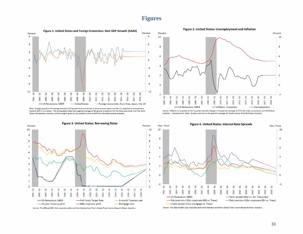
33
Figures
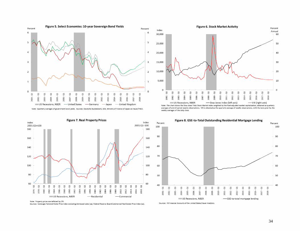
34
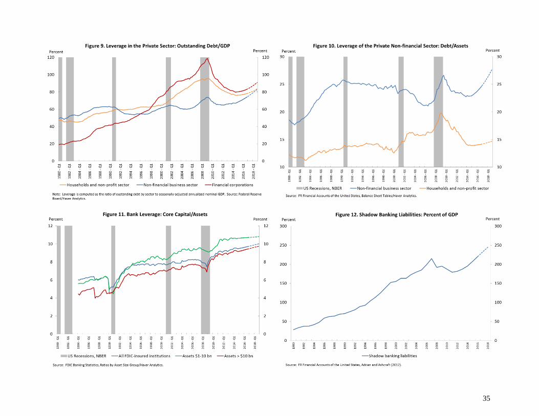
35

36
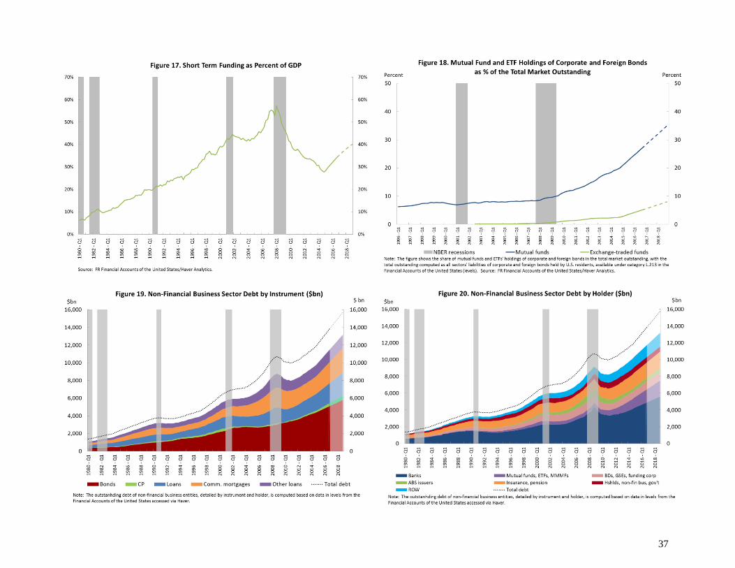
37

38
Tables
Table 1: Summary of Indicators and Risks Highlighted in the Hypothetical Scenario, by Sector
Risk →
Sector ↓ Asset Valuation Leverage Maturity Transformation
Non-financial
business
Term and credit spreads
Equity valuations
Commercial property prices
Debt-to-GDP
Debt-to-Assets
Household Mortgage spreads
Residential property prices
Debt-to-GDP
Debt-to-assets
GSE lending
Banking Debt-to-GDP
Capital ratios
High quality liquid asset share
Maturity mismatches
Non-bank
financial
Non-bank size Money market fund risks
Short term funding size
Repo funding backed by bonds
Bond mutual funds
Notes: The color code represents a suggestive assessment of risks in the hypothetical scenario provided by the authors ahead of the Tabletop Exercise, and
does not necessarily reflect the views that the Committee of Presidents members shared during the exercise, which are summarized in Section 4. Red
suggests relatively higher risk, and green suggests relatively lower risk. Yellow indicates moderate risk.

39
Table 2: Prudential Tools to Address Cyclical Changes in Financial Conditions
Prudential
Tools
Categories
Tools
Risks
Addressed
Applicable
Scenarios Can Target
Specific
Exposures?
Applicable
Banks / BHCs
Requires
Interagency
Agreement
Considerations44
Valuation (Val),
Leverage (Lev),
Mat & Liq (Liq)
Boom Bust
Capital
Regulation Leverage Ratios Lev X X
Minimum LR to all,
SLR to advanced
approaches45
X
Assume SLR effective by 2016Q4 for purposes of
tabletop exercise.
Countercyclical Buffers
(CCyB) Val, Lev X X46 ≥$250bn assets47 X
Increases are effective 12 months after announcement,
sooner in emergencies; decreases are effective
immediately.
Sectoral Risk Weights Val, Lev X X X All X
Liquidity
Regulation
Liquidity Coverage Ratio
(LCR) Liq X X48 ≥$50bn assets49 X
Net Stable Funding Ratio
(NSFR)50
Liq X X TBD X
Credit
Regulation
Loan-to-Value Ratio Val, Lev X X All X LTV have been implemented through guidance that can
be changed more expeditiously.
Margins Val, Lev X X All & non-banks Implement using Fed’s authority under the Securities
and Exchange Act of 1934.
Supervisory
Stress Test CCAR Val, Lev X X X BHCs ≥$50bn
assets
Annual frequency creates challenges. Targeting specific
exposures requires pre-announcing and/or repeating the
scenario.
CLAR Liq X X X BHCs in LISCC
portfolio51
Potential delayed impact due to CLAR messages being
delivered annually.
Supervisory Guidance Val, Lev, Liq X X X All
Moral Suasion Val, Lev, Liq X X X All
44
Most of the tools in this table are subject to a lag between the time policymakers decide to apply the tool and the time the tool becomes effective. In many
instances, this lag may arise from administrative processes. 45
Does not apply to bank holding companies with pro-forma consolidated assets of less than $1bn that meet several criteria. SLR applies to banks with ≥$250bn in
assets or ≥$10bn in foreign exposures and enhanced SLR apply to U.S. top-tier holding companies identified as G-SIBs. 46
The CCyB can be applied in downturn scenarios only if it has previously been activated to a non-zero level. 47
Also applies to banks with≥$10bn in foreign exposures. 48
Supervisors have discretion in determining timeframe for remediating an LCR shortfall. For the purposes of the tabletop, assume that the NSFR rule allows similar
discretion. 49
LCR applies to banks ≥$250bn in assets or ≥$10bn in foreign exposures. Modified LCR applies to banks ≥$50bn in assets. 50
For purposes of the tabletop exercise, assume that the NSFR is implemented similar to the LCR in the U.S. and is effective by 2016Q4. 51
See www.federalreserve.gov/bankinforeg/large-institution-supervision.htm for a current list of firms in the LISCC portfolio.
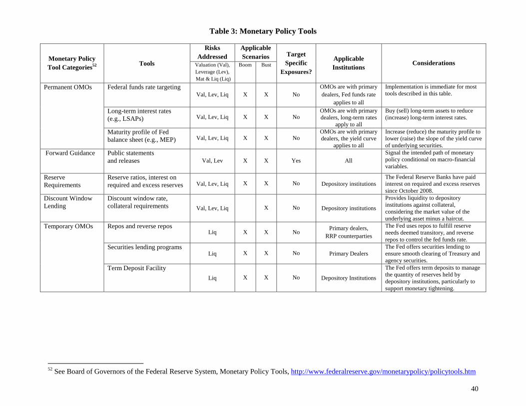
40
Table 3: Monetary Policy Tools
Monetary Policy
Tool Categories52
Tools
Risks
Addressed
Applicable
Scenarios Target
Specific
Exposures?
Applicable
Institutions Considerations Valuation (Val),
Leverage (Lev),
Mat & Liq (Liq)
Boom Bust
Permanent OMOs
Federal funds rate targeting Val, Lev, Liq X X No
OMOs are with primary
dealers, Fed funds rate
applies to all
Implementation is immediate for most
tools described in this table.
Long-term interest rates
(e.g., LSAPs) Val, Lev, Liq X X No OMOs are with primary
dealers, long-term rates
apply to all
Buy (sell) long-term assets to reduce
(increase) long-term interest rates.
Maturity profile of Fed
balance sheet (e.g., MEP) Val, Lev, Liq X X No OMOs are with primary
dealers, the yield curve
applies to all
Increase (reduce) the maturity profile to
lower (raise) the slope of the yield curve
of underlying securities.
Forward Guidance Public statements
and releases
Val, Lev X X Yes All
Signal the intended path of monetary
policy conditional on macro-financial
variables.
Reserve
Requirements
Reserve ratios, interest on
required and excess reserves Val, Lev, Liq X X No Depository institutions
The Federal Reserve Banks have paid
interest on required and excess reserves
since October 2008.
Discount Window
Lending
Discount window rate,
collateral requirements Val, Lev, Liq X No Depository institutions
Provides liquidity to depository
institutions against collateral,
considering the market value of the
underlying asset minus a haircut.
Temporary OMOs
Repos and reverse repos Liq X X No
Primary dealers,
RRP counterparties
The Fed uses repos to fulfill reserve
needs deemed transitory, and reverse
repos to control the fed funds rate.
Securities lending programs Liq X X No Primary Dealers
The Fed offers securities lending to
ensure smooth clearing of Treasury and
agency securities.
Term Deposit Facility
Liq X X No Depository Institutions
The Fed offers term deposits to manage
the quantity of reserves held by
depository institutions, particularly to
support monetary tightening.
52
See Board of Governors of the Federal Reserve System, Monetary Policy Tools, http://www.federalreserve.gov/monetarypolicy/policytools.htm


![Online video-publication for biological research [Cr3 900 Pritsker]](https://img.dokumen.tips/doc/110x75/554935a6b4c905054d8b46a6/online-video-publication-for-biological-research-cr3-900-pritsker.jpg)