Embed Size (px)
Citation preview

Macroeconomics in the World Economy:Theory and ApplicationsTopic 2: The Supply Side
Dennis Plott
University of Illinois at ChicagoDepartment of Economics
http://blackboard.uic.edu
Spring 2014
Plott (ECON 221) Spring 2014 1 / 71

Outline
1 Topic 2: The Supply Side of the EconomyThe Production Market
The Labor MarketLabor Demand
Labor Supply
Long-Run Aggregate Supply
Long-Run Economic Growth
Plott (ECON 221) Spring 2014 2 / 71

Topic 2 Readings & Goals
Readings1 ABC 8e (2014) Chapter 32 ABC 8e (2014) Chapter 6
Goals1 Introduce the supply side of the macro economy.2 Discuss how countries grow and why some countries grow faster than
others.3 Determine how wages are set in the labor market.
Plott (ECON 221) Spring 2014 3 / 71

Outline
1 Topic 2: The Supply Side of the EconomyThe Production Market
The Labor MarketLabor Demand
Labor Supply
Long-Run Aggregate Supply
Long-Run Economic Growth
Plott (ECON 221) The Production Market Spring 2014 4 / 71

Factors of Production
Capital (K ): tools, machines, and structures used in production
Labor (N): the physical and mental efforts of workers
Others (raw materials, land, energy)
Productivity of factors depends on technology and management
Plott (ECON 221) The Production Market Spring 2014 5 / 71

The Production Function
It’s the mapping of inputs into output. GDP (Y ) is produced with
capital (K , price weighted) and labor (N , hours):
Y = AF(K ,N)
Sometimes, I will modify the production function such that:
Y = AF(K ,N ,other inputs)
where other inputs include energy/oil
Exhibits constant returns to scale (CRS).
A realistic example is the Cobb-Douglas function for F(K ,N):
Y = AK aN1−a
Y = AK 0.3N0.7
A is Total Factor Productivity (TFP), an index of efficiency in the use of
inputs (technology). 0 < a < 1 capital share.
Plott (ECON 221) The Production Market Spring 2014 6 / 71

Two Measures of Productivity
Labor Productivity = YN = A
( KN
)0.3
Driven by A and KN
Total Factor Productivity (TFP) = A = YF(K ,N)
Basically TFP is a "catch-all" for anything that effects output otherthan K and N .
Workweek of labor and capitalQuality of labor and capitalRegulationInfrastructureCompetitionSpecializationInnovationStrategy (Entrepreneurial methods/new management techniques)
Some components of TFP tend to be procyclical
Definition of procyclical: Variable increases when Y is high, decreases
when Y is lowPlott (ECON 221) The Production Market Spring 2014 7 / 71
Measurement
Y is GDP (it is measured in real dollars). As noted above, we want to
measure Y in "real" dollars.
For our Cobb-Douglas production function (previous slide), K ismeasured in real dollars and N in terms of hours worked.
K often is measured as the replacement cost of capitalN often is measured in number of workers time hours per worker
However, in practice, N can be measured in different ways (number ofworkers, number of effective workers, production workers).
Hours worked takes into account part-time and full-time. Number ofeffective workers adjustment are made by BLS.Unskilled vs.skilled workers: "skill" differentials.
Note: When we talk about standard of livings: income per capita is YPop
where Y is income and Pop is a population measure – sometimes we
assume Pop = N , labor force.
Plott (ECON 221) The Production Market Spring 2014 8 / 71

The Aggregate Production Function
To build intuition let’s represent the production function graphically.
Hold A and N constant.
Graph Y and K : level of output that can be produced at each level of K .
K
Y
Y = AF(K ,N)
Increasing capital (K ) increases output (Y ).
However increasing K of the same quantity produces smaller and smaller
increases in output. Marginal product of capital (MPK ) is decreasing (curve
flattens).
Plott (ECON 221) The Production Market Spring 2014 9 / 71

Example: Why are Marginal Products of FactorsDecreasing?
Consider a Iron Ore Mine where the only inputs are Excavators (K ) and
Miners (N).
Suppose 10 miners work at the mine.
Start with no excavators, output is 0. They cannot dig.
When we add 1 excavator output is going to be low (miners can only use 1
machine to excavate) but positive. That single excavator is likely to be
used fully (everybody has to wait in line to use it and it never sits idle).
Suppose now the mine acquires another 10 excavators. Output is going to
be higher and now the time waiting to use the excavator is going to be
zero. However 1 excavator is going sit idle (and maybe used as
replacement when another one breaks down). Adding additional
excavators increases output but at slower and slower rate.
Fixing A and N , MPK falls when K increases
Plott (ECON 221) The Production Market Spring 2014 10 / 71

The Aggregate Production Function (Continued)
Now hold A and K fixed.
Graph Y and N
A different slope than the previous graph (steeper because 1−a > a).
N
Y
Y = AF(K ,N)
Increasing labor (N) increases output (Y ).
Increasing N of the same quantity produces smaller and smaller increases
in output. Marginal product of labor (MPN) is decreasing (curve flattens).
Plott (ECON 221) The Production Market Spring 2014 11 / 71

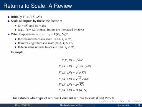
Returns to Scale: A Review
Initially Y1 = F(K1,N1)Scale all inputs by the same factor z:
K2 = zK1 and N2 = zN1
(e.g., if z = 1.2, then all inputs are increased by 20%)
What happens to output, Y2 = F(K2,N2)?
If constant returns to scale (CRS), Y2 = zY1
If increasing returns to scale (IRS), Y2 > zY1
If decreasing returns to scale (DRS), Y2 < zY1
Example:
F(K ,N) =pKN
F(zK ,zN) =√
(zK )(zN)
F(zK ,zN) =√
z2KN
F(zK ,zN) =√
z2p
KN
F(zK ,zN) = zp
KN
F(zK ,zN) = zF(K ,N)
This exhibits what type of returns?
Constant returns to scale (CRS) ∀z > 0
Plott (ECON 221) The Production Market Spring 2014 12 / 71
Returns to Scale: A Review
Initially Y1 = F(K1,N1)Scale all inputs by the same factor z:
K2 = zK1 and N2 = zN1
(e.g., if z = 1.2, then all inputs are increased by 20%)
What happens to output, Y2 = F(K2,N2)?
If constant returns to scale (CRS), Y2 = zY1
If increasing returns to scale (IRS), Y2 > zY1
If decreasing returns to scale (DRS), Y2 < zY1
Example:
F(K ,N) =pKN
F(zK ,zN) =√
(zK )(zN)
F(zK ,zN) =√
z2KN
F(zK ,zN) =√
z2p
KN
F(zK ,zN) = zp
KN
F(zK ,zN) = zF(K ,N)
This exhibits what type of returns? Constant returns to scale (CRS) ∀z > 0
Plott (ECON 221) The Production Market Spring 2014 12 / 71

Marginal Product of Labor
Plott (ECON 221) The Production Market Spring 2014 13 / 71

Marginal Product of Labor: a Decrease in TFP (A)
Plott (ECON 221) The Production Market Spring 2014 14 / 71

Outline
1 Topic 2: The Supply Side of the EconomyThe Production Market
The Labor MarketLabor Demand
Labor Supply
Long-Run Aggregate Supply
Long-Run Economic Growth
Plott (ECON 221) The Labor Market Spring 2014 15 / 71

Labor Market Roadmap: Demand and Supply
Three main concepts:1 Firms decide the optimal amount of labor to hire: Firm Labor Demand.
If you aggregate (i.e. add up) those decisions you obtain the AggregateLabor Demand.
2 Individual decision on optimal amount of leisure (= 1−N) to consume(and hence how much to work): Individual Labor Supply.If you aggregate those decisions you obtain the Aggregate Labor Supply.
3 Classical representation of the Labor Market Equilibrium:Aggregate Labor Demand = Aggregate Labor Supply
Note: no unemployment (real wages can adjust).
Plott (ECON 221) The Labor Market Spring 2014 16 / 71

Labor Demand: Firm’s Profit Maximizing Decision
In a competitive market, a firm can sell as much Y as it wants at the going price
P, and can hire as much N as it wants at the going nominal wage W .
Facing W and P, a profit maximizing firm will hire N to the point were MPN = WP
(the benefit from an additional worker (in terms of additional output) must equal
the cost which they are paid). This is straight from Microeconomics)
Why is this optimal? The MPN is decreasing in N , so:
If MPN > W /P then the firm can increase profits by increasing N . (Intuition: the
new worker adds more value than he costs, so profits increase).
If MPN < W /P then the firm can increase profits by decreasing N. (Intuition:
letting go a worker reduces the wage bill more than it cuts production, so profits
increase).
Example:
With Cobb-Douglas production function: MPN = 0.7Y
N= 0.7A
(K
N
)0.3
If firms maximize profits, then:W
P= 0.7
Y
N= 0.7A
(K
N
)0.3
Plott (ECON 221) The Labor Market Spring 2014 17 / 71
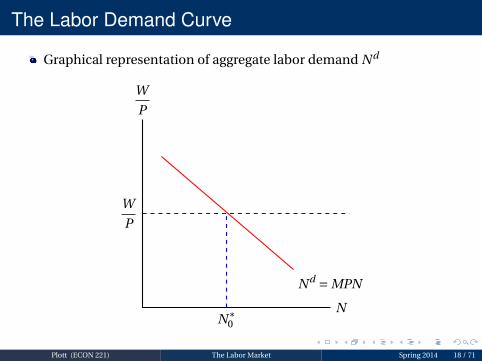
The Labor Demand Curve
Graphical representation of aggregate labor demand Nd
N
W
P
Nd = MPN
W
P
N∗0
Plott (ECON 221) The Labor Market Spring 2014 18 / 71

Notes on the Labor Demand Curve
Let us consider the level of K fixed for now.
Nd slopes downward: Nd = MPN = (1−a)A
(K
N
)a
= 0.7A
(K
N
)0.3
Nd rises with A and K .
When A increases, all my inputs are more productive, so the marginalproduct of one extra unit of labor input is higher.When K is higher, I have more capital to use with my labor (one extraunit of labor can work with more capital), hence the marginal productof labor is higher.
Note: labor demand shifts when the aggregate production changes (we
will see that the aggregate supply shifts).
Caveat: Who says that there is a demand for more Y ?
Need to look at the demand side of economy (introduced in Topic 1 –discussed in depth throughout the course).
Plott (ECON 221) The Labor Market Spring 2014 19 / 71

Labor Supply: Individual Utility Maximization
Labor Supply (N s) results from individual optimization decisions.
Households compare benefits of working (additional lifetime
resources) with cost of working (forgone leisure).
Question: how does the supply of labor moves with a change in real
wages
(W
P
)?
1 The income effect says that as people become richer they want toconsume more of all goods, that includes leisure, so they work less.
2 The substitution effect says that as the price of a good goes up todayrelative to another one you want to consume less of that good. The priceof leisure is the wage you forego not to work.
Plott (ECON 221) The Labor Market Spring 2014 20 / 71
Review of Individual Labor Supply
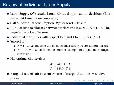
Labor Supply (N s) results from individual optimization decisions (This
is straight from microeconomics.)
Call C individual consumption, P price level, L leisure.
1 unit of time to allocate between work N and leisure L. N = 1−L. The
wage is the price of leisure!
Individual maximizes with respect to C and L her utility U(C,L)Subject to:
N = 1−L (i.e. the time you do not work is what you consume as leisure)W (1−L) = P ·C (i.e. labor income = consumption; simple static budgetconstraint)
Her optimal choice gives:
W
P= MUL(C,L)
MUC(C,L)
Marginal rate of substitution (= ratio of marginal utilities) = relative
prices.
Plott (ECON 221) The Labor Market Spring 2014 21 / 71

Review of a Simple Individual Labor Supply
Her optimal choice is:
W
P= MUL(C,L)
MUC(C,L)
Marginal rate of substitution (= ratio of marginal utilities) = relative prices.
If WP goes up, then MUL(C,L)
MUC (C,L) has to go up.
QUESTION: Is N(= 1−L) going to increase or decrease?
Recall first that marginal utility of a good goes down with the amount
consumed (the 10th hamburger is not as satisfying as the 1st).
Substitution effect: if real wage goes up you work more. MUL(C,L)
increases – consume less leisure and MUC(C,L) decreases – consume more
goods).
Income effect: if real wage goes up you work less. MUL(C,L) decreases –
consume more leisure and MUC(C,L) decreases even more – consume
more goods).
Plott (ECON 221) The Labor Market Spring 2014 22 / 71

Factors Affecting Labor Supply
Income effect and substitution effect are ambiguous if changes inW
Pare permanent.
Simplify: assign all the income effect to changes in Present Value of
Lifetime Resources (PVLR) and we focus on a positively sloped N s
(only substitution effect).
Factors Affecting Labor Supply:
The Current Real Wage
(W
P
).
But also Future Real Wages through the Household’s Present Value ofLifetime Resources (PVLR).The Marginal Tax Rate on Labor Income (τn) – leisure is more/lesscostly.The Marginal Tax Rate on Consumption (τc) – consumption ismore/less costly.Value of Leisure (reservation wage) – non-work status (VL).The Working Age Population (pop).
Plott (ECON 221) The Labor Market Spring 2014 23 / 71

The Labor Supply Curve
Graphical representation of aggregate labor supply N s
NS(PVLR,τc,τn,population,Value of Leisure)
N
W
P
N s(·)
Ns slopes upward due to the substitution effect of before-tax wages
Plott (ECON 221) The Labor Market Spring 2014 24 / 71
Labor Supply Curve Notes
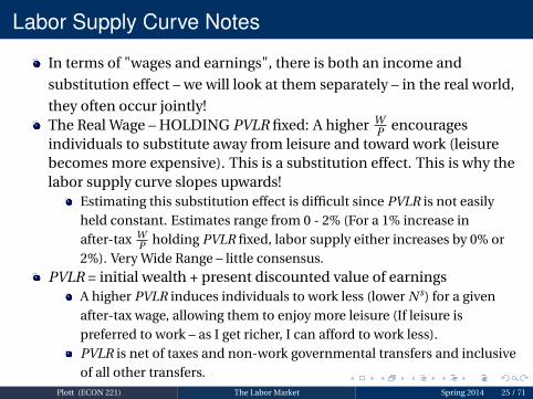
In terms of "wages and earnings", there is both an income and
substitution effect – we will look at them separately – in the real world,
they often occur jointly!The Real Wage – HOLDING PVLR fixed: A higher W
P encouragesindividuals to substitute away from leisure and toward work (leisurebecomes more expensive). This is a substitution effect. This is why thelabor supply curve slopes upwards!
Estimating this substitution effect is difficult since PVLR is not easilyheld constant. Estimates range from 0 - 2% (For a 1% increase inafter-tax W
P holding PVLR fixed, labor supply either increases by 0% or2%). Very Wide Range – little consensus.
PVLR = initial wealth + present discounted value of earningsA higher PVLR induces individuals to work less (lower N s) for a givenafter-tax wage, allowing them to enjoy more leisure (If leisure ispreferred to work – as I get richer, I can afford to work less).PVLR is net of taxes and non-work governmental transfers and inclusiveof all other transfers.
Plott (ECON 221) The Labor Market Spring 2014 25 / 71

Labor Supply Curve Notes (Continued)
Marginal tax rate on labor income – Should have same substitution
effect as the before tax real wage. Studies of the 1986 U.S. Tax Reform
found that only high-earning married women worked more in
response to lower marginal income tax rates.
Marginal tax rate on consumption – see above
Her optimal choice with taxes:
W (1−τn)
P(1+τc)= MUL(C,L)
MUC(C,L)
Value of Leisure (VL) – If leisure/no-work becomes more/less
attractive, households will work less/more (reservation wage).
(Welfare programs, child care, etc.).
Working Age Population (pop): Usually defined as 16–64; includes
changes in Labor Force Participation Rates.
Plott (ECON 221) The Labor Market Spring 2014 26 / 71

Labor Market Equilibrium
N
W
P
N s(PVLR,τn,τc,pop,VL)
Nd(A,K )
N0
(W
P
)0
Plott (ECON 221) The Labor Market Spring 2014 27 / 71

Example 1: Temporary Increase in A
N
W
P
N s(PVLR,τn,τc,pop,VL)
Nd(A,K )
N0
(W
P
)0
Plott (ECON 221) The Labor Market Spring 2014 28 / 71
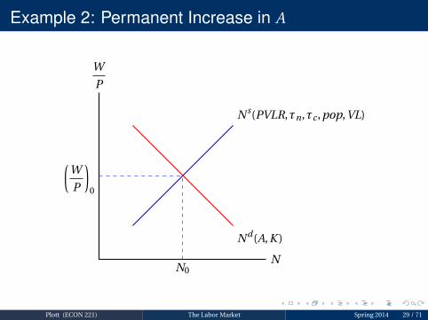
Example 2: Permanent Increase in A
N
W
P
N s(PVLR,τn,τc,pop,VL)
Nd(A,K )
N0
(W
P
)0
Plott (ECON 221) The Labor Market Spring 2014 29 / 71
Interpretation
If firms become more productive they demand more labor. The Nd
curve shifts rightward. Real wages increase from the initial level since
workers become scarce. However PVLR stays the same so no
movement of N s. Then if the productivity shock is temporary,
everything reverts back.
If the shift is permanent people are also permanently "richer", so an
increase in PVLR will produce a consequent shift leftward of the N s
curve (income effect). This leaves the final result ambiguous.
Note: for any question involving the labor market I will specify
whether the income or substitution effect dominates.
Plott (ECON 221) The Labor Market Spring 2014 30 / 71

Example 3: Permanent Increase in Population
N
W
P
N s(PVLR,τn,τc,pop,VL)
Nd(A,K )
N0
(W
P
)0
Plott (ECON 221) The Labor Market Spring 2014 31 / 71

Consumption and Labor Taxes
Marginal tax rate on labor income – people care about after-tax wage
W (1−τn).
Consumption taxes – people care about after-tax price P(1+τC).
While the substitution effect of changing before-tax wage causes a
movement along the supply curve, the substitution effect of changing
taxes causes the labor supply curve to shift.
If leisure becomes relatively more inexpensive than consumption
(labor taxes or consumption taxes increase), the N s shifts to the left.
If the shift is permanent people are also permanently "poorer", so a
drop of PVLR will go down with consequent shift right of the N s curve
(income effect). This leaves the final result ambiguous.
Plott (ECON 221) The Labor Market Spring 2014 32 / 71

Example 4: Temporary Increase in Taxes (τc or τn)
N
W
P
N s(PVLR,τn,τc,pop,VL)
Nd(A,K )
N0
(W
P
)0
Plott (ECON 221) The Labor Market Spring 2014 33 / 71

Example 5: Permanent Increase in Taxes (τc or τn)
N
W
P
N s(PVLR,τn,τc,pop,VL)
Nd(A,K )
N0
(W
P
)0
Plott (ECON 221) The Labor Market Spring 2014 34 / 71

Recap on Labor Supply
Substitution Effect:For a given PVLR, a higher after-tax wage increases N s.
This is why Labor Supply Curve slopes upward
Income Effect:
For a given after-tax wage, higher PVLR decreases N s.Evidence:
Weak consensus is that, with equal (%) increase in PVLR and the after-tax
wage, Ns falls (income effect dominates).
A must read: Chapter 3 (on labor markets) in the text book.
Plott (ECON 221) The Labor Market Spring 2014 35 / 71

Labor Market Equilibrium (in the Long-Run)
We define Long-run Equilibrium in macroeconomics as occurring
when the labor market clears.
By definition, long-run macro equilibrium exists when N = N .
At N , labor demand = labor supply. So, by definition, all workers whowant a job (the suppliers) are able to find a firm looking for a worker(the demanders).
Implies that cyclical unemployment = zero at N .Long-run equilibrium is characterized by zero cyclical unemployment.
It is an equilibrium in that there is no incentive for real wages tochange at N .
Real wages( W
P
)has two components: nominal wages (W ) and the price
level (P).
Note: Y (by definition) = AK 0.3(N)0.7
Y = long-run equilibrium level of output (where labor market is in
equilibrium)
Plott (ECON 221) The Labor Market Spring 2014 36 / 71

Outline
1 Topic 2: The Supply Side of the EconomyThe Production Market
The Labor MarketLabor Demand
Labor Supply
Long-Run Aggregate Supply
Long-Run Economic Growth
Plott (ECON 221) Long-Run Aggregate Supply Spring 2014 37 / 71

Our First Aggregate Supply Curve
Suppose prices (P) increase. What happens in the labor market in thelong-run?
In terms of equilibrium, nothing happens!Increasing prices have no effect on labor demand (A and K do not change).Increasing prices have no effect on labor supply (VL, taxes, population, etc.do not change).
You may ask "Doesn’t PVLR change when prices increase?" No!
As long as nominal wages adjust, real wages will be unchanged when Pincreases.The % change in prices will be match exactly by the % change in nominalwages – real wages will not change (so PVLR will not change).No effect on labor supply.
Key: Because real wages will not change, changes in prices will have NO
effect on the labor market (i.e. it will have no effect on N) in the long-run.
Conclusion: changing prices will have NO effect on Y (since N is
constant) in the long-run.
Plott (ECON 221) Long-Run Aggregate Supply Spring 2014 38 / 71

Our First Aggregate Supply Curve
If the labor market clears, changes in prices will lead to equal changes in nominal wages. As aresult, there will be no change in N and hence, no change in Y .
This results in a vertical long-run aggregate supply (LRAS) curve. Prices do not affect productionin the long-run!
Y
P
LRAS
Y
Plott (ECON 221) Long-Run Aggregate Supply Spring 2014 39 / 71
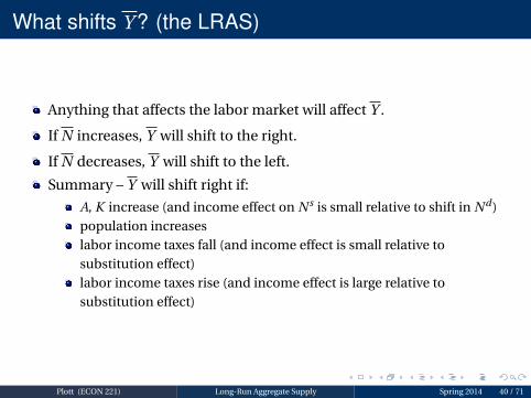
What shifts Y ? (the LRAS)
Anything that affects the labor market will affect Y .
If N increases, Y will shift to the right.
If N decreases, Y will shift to the left.
Summary – Y will shift right if:
A, K increase (and income effect on N s is small relative to shift in Nd)population increaseslabor income taxes fall (and income effect is small relative tosubstitution effect)labor income taxes rise (and income effect is large relative tosubstitution effect)
Plott (ECON 221) Long-Run Aggregate Supply Spring 2014 40 / 71

Things to Remember!
The demand side of the economy is NOT important for determining Y .
All we need to know is A, K and N and we know Y .The demand side of the economy is not important for economic growth.Key: If I ever ask you about what determines Y (i.e.,output/income/expenditure in the long-run), you should think about A,K and the labor market.
As a rule, K will be fixed unless I tell you otherwise (for simplicity, you will
see why soon).
Why do we care about the demand side of the economy?
In the long-run, prices will be determined by demand.Also, LRAS is dependent on labor market being in equilibrium. In theshort-run, the labor market need not be in equilibrium.Demand will determine output in the short-run.
Plott (ECON 221) Long-Run Aggregate Supply Spring 2014 41 / 71

Summary
In the long-run – when labor markets clear:
Supply side of economy (labor market, K , A, other inputs like oil)determines output.Demand side of economy (C + I +G+NX) will determine prices.
In the short-run – when labor markets do not clear:
Demand and Supply jointly determine prices and output.
Three outstanding issues (we will get to them soon):
When is the labor market NOT in equilibrium?What does the supply curve look like when labor market doesn’t clear?What determines demand?
Plott (ECON 221) Long-Run Aggregate Supply Spring 2014 42 / 71
When Are Labor Markets in Dis-equilibrium?
The labor market is in disequilibrium when labor demand is not equal
to labor supply.
Nominal wages do not adjust to clear the labor market.
We refer to this as "sticky" or "rigid" wages.Because of wage contracts (and uncertainty), nominal wages no notalways adjust immediately.Need a model for short-run disequilibrium – we will do that in Topic 6.
Plott (ECON 221) Long-Run Aggregate Supply Spring 2014 43 / 71

Cyclical Unemployment in Labor Markets
When do we get cyclical unemployment in our models?
Cyclical unemployment occurs when there are no jobs available (labor demand) for those withthe skills and the desire to work (labor supply) at current wages.
Cyclical unemployment occurs only in disequilibrium (when desired labor demand less thandesired labor supply – at given wages)
N
W
P
Ns0
Nd0
N0
(W
P
)0
a
Plott (ECON 221) Long-Run Aggregate Supply Spring 2014 44 / 71

Outline
1 Topic 2: The Supply Side of the EconomyThe Production Market
The Labor MarketLabor Demand
Labor Supply
Long-Run Aggregate Supply
Long-Run Economic Growth
Plott (ECON 221) Long-Run Economic Growth Spring 2014 45 / 71

Why Growth Matters
Anything that effects the long-run rate of economic growth – even by a
tiny amount – will have huge effects on living standards in the
long-run.
Annual Growth Rateof
Income per Capita
Increase in
Standard of Livingafter . . .
. . . 25 Years . . . 50 Years . . . 100 Years
2.0% 64.0% 169.2% 624.5%
2.5% 85.4% 243.7% 1,081.4%
Example:
Korea and the Philippines had the same level of real income per capitain 1965.By 2010, Korea’s real income per capita was six times that of thePhilippines thanks to Korea’s rapid economic growth.
Plott (ECON 221) Long-Run Economic Growth Spring 2014 46 / 71
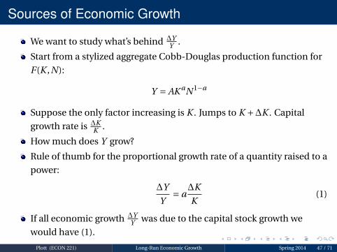
Sources of Economic Growth
We want to study what’s behind ∆YY .
Start from a stylized aggregate Cobb-Douglas production function for
F(K ,N):
Y = AK aN1−a
Suppose the only factor increasing is K . Jumps to K +∆K . Capital
growth rate is ∆KK .
How much does Y grow?
Rule of thumb for the proportional growth rate of a quantity raised to a
power:
∆Y
Y= a
∆K
K(1)
If all economic growth ∆YY was due to the capital stock growth we
would have (1).
Plott (ECON 221) Long-Run Economic Growth Spring 2014 47 / 71

Sources of Economic Growth (Continued)
Similarly consider all growth is due to an increase in labor N +∆N
Same rule would deliver:
∆Y
Y= (1−a)
∆N
N(2)
Now consider an increase in TFP A+∆A
Same rule would deliver:
∆Y
Y= ∆A
A(3)
So how much does Y grows when everything can change?
Simple: add (1), (2), (3) together!
∆Y
Y= a
∆K
K+ (1−a)
∆N
N+ ∆A
A
Identifies the three main components that account for output growth.
Growth accounting.Plott (ECON 221) Long-Run Economic Growth Spring 2014 48 / 71

Growth Accounting
Y = AK 0.3N0.7 (US production function) implies:
∆Y
Y= 0.3
∆K
K+0.7
∆N
N+ ∆A
A
Output in a country can be decomposed in:
Growth in TFP (entrepreneurial ability, education, roads, technology,etc.)Growth in Capital (machines, equipment, plants, etc.)Growth in Labor (workforce, population, labor participation, etc.).
Note: For a general production function (i.e. not Cobb-Douglas)
∆Y
Y= aK
∆K
K+aN
∆N
N+ ∆A
A
where aK = elasticity of output with respect to capital (same definition
for labor).
Plott (ECON 221) Long-Run Economic Growth Spring 2014 49 / 71

Limits of Growth Accounting: Just Diagnostics
. . . these accounting exercises say nothing about causality, and so are
very hard to interpret.
Say you found it’s 50% efficiency and 50% factor endowments. What
conclusion do you draw from it? You could imagine a story where the
underlying cause of growth is factor accumulation, with
technological upgrading or enhanced allocative efficiency as the
by-product.
Or you could imagine a story whereby technological change is the
driver behind increased accumulation.
Both are compatible with the result from accounting decomposition.
Indeed, I have yet to see a sources-of-growth decomposition which
answers a useful and relevant economic or policy question.
Dani Rodrik (KSG, Harvard)
http://rodrik.typepad.com/dani_rodriks_weblog/2008/02/
what-use-is-sou.html
Plott (ECON 221) Long-Run Economic Growth Spring 2014 50 / 71

Long-Run Growth
Two basic questions about growth:1 What’s the relationship between the long-run standard of living and the
saving rate, population growth rate, and rate of technical progress?2 How does economic growth change over time? Will it speed up, slow
down, or stabilize?
We will use the Solow Growth model to explore these questions.
Plott (ECON 221) Long-Run Economic Growth Spring 2014 51 / 71

The Solow Growth Model: Assumptions
A worker is a worker. Assume equal qualifications (homogeneous labor)
A unit of capital is a unit of capital, no matter what it actually is (homogeneous
capital).
K is no longer fixed: investment causes it to grow, depreciation causes it to
shrink.
Technology is just the function that connects K and N to Y . An engineering
blueprint.
There’s no unemployment (or it doesn’t change)
Constant returns to scale (CRS)
The economy is closed (i.e. NX = 0) and the asset market clears, so It = St ; i.e.
national saving equals investment.
G = T = 0 only to simplify presentation; we can still do fiscal policy experiments.
Population and work force grow at same rate∆Nt
Nt= n (exogenous)
Example: Suppose N = 1,000 in year 1 and the population is growing at 2% per year(n = 0.02).Then ∆N = nN = 0.02×1,000 = 20, so N = 1,020 in year 2.
Plott (ECON 221) Long-Run Economic Growth Spring 2014 52 / 71

The Solow Model
Due to Robert Solow (1924 – ), won Nobel Prize (1987) for
contributions to the study of economic growth.A major paradigm:
widely used in policy makingbenchmark against which most recent growth theories are compared
Looks at the determinants of economic growth and the standard of
living in the long-runhttp://www.nobelprize.org/nobel_prizes/economic-sciences/laureates/1987/solow-facts.html
Plott (ECON 221) Long-Run Economic Growth Spring 2014 53 / 71
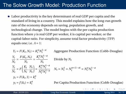
The Solow Growth Model: Production Function
Labor productivity is the key determinant of real GDP per capita and thestandard of living in a country. This model explains how the long-run growthrate of the economy depends on saving, population growth, andtechnological change. The model begins with the per capita productionfunction where y is real GDP per worker, k is capital per worker, or thecapital-labor ratio. For simplicity, assume total factor productivity (TFP)equals one; i.e. A = 1:
Yt = F(Kt ,Nt ) = K at N1−a
t Aggregate Production Function (Cobb-Douglas)
Yt
Nt= F(Kt ,Nt )
Nt= K a
t N1−at
NtDivide by Nt
Yt
Nt= F
(Kt
Nt,
Nt
Nt
)= K a
t N1−at
Nat N1−a
t
Nt = N1t = Na+(1−a)
t = Nat N1−a
t
yt = F(kt ,1) = kat
yt = f (kt ) = kat Per Capita Production Function (Cobb-Douglas)
Plott (ECON 221) Long-Run Economic Growth Spring 2014 54 / 71

The Solow Growth Model: Capital Accumulation
Capital accumulation is the change over time in the capital stock. The capitalstock increases because of investment in new capital, but it also decreasesbecause of depreciation and dilution. Under the simplifying assumption of aclosed economy with no government sector, all output is either consumed orinvested in new capital goods. Real GDP per worker, y, can be divided intoconsumption per worker, c, and investment per worker, i:
Yt = Ct + It +Gt +NXt Aggregate Income-Expenditure Equation
Yt = Ct + It G = T = 0 and NX = 0 (Assumed)
Yt
Nt= Ct
Nt+ It
NtDivide by Nt
yt = ct + it Per Capita Form
Note: it is investment per capita NOT the nominal interest rate!
Plott (ECON 221) Long-Run Economic Growth Spring 2014 55 / 71
The Solow Growth Model: Saving
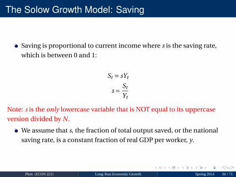
Saving is proportional to current income where s is the saving rate,
which is between 0 and 1:
St = sYt
s = St
Yt
Note: s is the only lowercase variable that is NOT equal to its uppercase
version divided by N .
We assume that s, the fraction of total output saved, or the national
saving rate, is a constant fraction of real GDP per worker, y.
Plott (ECON 221) Long-Run Economic Growth Spring 2014 56 / 71

The Solow Growth Model: Capital Accumulation
The capital-labor ratio, k, increases when the stock of investment goodsincreases faster than the number of workers. Because saving and investmentare equal, investment per worker, i, equals:
It = St
it = syt plug in St = sYt
ct = (1− s)yt substitute into yt = ct + it
Substituting the production function into the equation for investment, wehave the investment function: it = syt = sf (kt )
As the capital-labor ratio increases, real GDP per worker increases, causinginvestment per worker to increase. Because of diminishing marginal returns,increasing the capital-labor ratio causes smaller and smaller increases in realGDP per worker. Investment per worker equals the constant saving ratemultiplied by real GDP per worker, so the increase in investment per workergets smaller and smaller as the capital-labor ratio increases.
Plott (ECON 221) Long-Run Economic Growth Spring 2014 57 / 71
The Solow Growth Model: Depreciation and Dilution
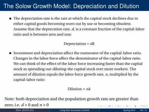
The depreciation rate is the rate at which the capital stock declines due toeither capital goods becoming worn out by use or becoming obsolete.Assume that the deprecation rate, d, is a constant fraction of the capital-laborratio and is between zero and one:
Depreciation = dk
Investment and depreciation affect the numerator of the capital-labor ratio.Changes in the labor force affect the denominator of the capital-labor ratio.We can think of the effect of the labor force increasing faster than the capitalstock as spreading out-diluting-the capital stock over more workers. Theamount of dilution equals the labor force growth rate, n, multiplied by thecapital-labor ratio:
Dilution = nk
Note: both depreciation and the population growth rate are greater than
zero; i.e. d > 0 and n > 0Plott (ECON 221) Long-Run Economic Growth Spring 2014 58 / 71

The Solow Growth Model: Equation of Motion
What determines next periods capital-labor ratio (kt+1)? There is a
base or stock of capital initially. This can be added to, subtracted from,
or maintained thereby determining if the future capital-labor ratio will
increase, decrease, or remain the same respectively.
kt+1 = kt + it −nkt −dkt
kt+1 −kt = it −nkt −dkt Subtract kt from both sides
∆kt = it −nkt −dkt ∆kt = kt+1 −kt
∆kt = it − (n+d)kt Collect like terms
∆kt = syt − (n+d)kt Substitute it = syt = sf (kt)
∆kt = sf (kt)− (n+d)kt Equation of Motion
Plott (ECON 221) Long-Run Economic Growth Spring 2014 59 / 71

The Solow Growth Model: Steady State
In the Solow growth model, equilibrium occurs when the capital-labor
ratio is constant; real GDP is also constant. An equilibrium in the
Solow growth model in which the capital-labor ratio and real GDP per
worker are constant, but capital, labor and output are growing, is
called a steady state.
∆kt = sf (kt)− (n+d)kt Equation of Motion
∆kt = 0 = sf (kt)− (n+d)kt In steady state
sf (k∗) = (n+d)k∗ An asterisk denotes steady state
Plott (ECON 221) Long-Run Economic Growth Spring 2014 60 / 71

The Solow Growth Model: Determinants – Saving
Higher saving rate means higher capital-labor ratio, higher output per
worker, and higher consumption per worker
Should a policy goal be to raise the saving rate?
Not necessarily, since the cost is lower consumption in the short-runThere is a trade-off between present and future consumption
Steady state values differ across countries. Government policies that
change the saving rate have a level effect – that is, the policies can raise
real GDP per capita and the standard of living to a higher level, but do
not have a growth effect: The policies will not result in a sustained
increase in the standard of living over time. Only policies that change
the steady-state growth rate of real GDP per worker have a growth
effect that will bring about sustained increases in the standard of
living.
Plott (ECON 221) Long-Run Economic Growth Spring 2014 61 / 71

The Solow Growth Model: The Golden Rule
While a higher capital stock implies higher output, this does not mean
that a higher capital stock is necessarily desirable. To sustain a high
level of the capital stock, a lot of output may have to be devoted to
replacement investment, so it will not be available for consumption.
We now compare steady states in terms of consumption. The steady
state with the highest possible level of consumption is known as the
golden rule level of capital accumulation. The golden rule can be
analyzed without reference to people’s behavior (that is, without
reference to the saving rate).Transition to the golden rule steady state:
The economy does NOT have a tendency to move toward the goldenrule steady state.Achieving the golden rule requires that policymakers adjust s.This adjustment leads to a new steady state with higher consumption.But what happens to consumption during the transition to the goldenrule?
Plott (ECON 221) Long-Run Economic Growth Spring 2014 62 / 71

Edmund Phelps (1933 – )
Nobel Prize (2006)
Developed golden rule level of capital accumulation.
Edmund Phelps helped change the way we think about
macroeconomic theory and policy, by introducing imperfect
information and costly communication into the theory, and deriving
their implications for the dynamics of inflation and unemployment.http://www.nobelprize.org/nobel_prizes/economic-sciences/laureates/2006/phelps-facts.html
Plott (ECON 221) Long-Run Economic Growth Spring 2014 63 / 71

The Solow Growth Model: Determinants – PopulationGrowth
Higher population growth means a lower capital-labor ratio, lower
output per worker, and lower consumption per worker .
Should a policy goal be to reduce population growth?
Doing so will raise consumption per workerBut it will reduce total output and consumption, affecting a nation’sability to defend itself or influence world events
The Solow model also assumes that the proportion of the populationof working age is fixed
But when population growth changes dramatically this may not be trueChanges in cohort sizes may cause problems for social security systemsand areas like health care
Plott (ECON 221) Long-Run Economic Growth Spring 2014 64 / 71
The Malthusian Model (1798)
Thomas Robert Malthus (1766–1834) argued in his book An Essay on the
Principle of Population as It Affects the Future Improvement of Society that
an ever-increasing population would continually strain society’s ability to
provide for itself. Mankind, he predicted, would forever live in poverty.
Malthus began by noting that "food is necessary to the existence of man"
and that "the passion between the sexes is necessary and will remain
nearly in its present state". He concluded that "the power of population is
infinitely greater than the power in the earth to produce subsistence for
man". According to Malthus, the only check on population growth was
"misery and vice".
Malthus neglected the effects of technological progress; e.g. birth control.
Since Malthus, world population has increased sixfold, yet living standards
are higher than ever.
http://www.econlib.org/library/Malthus/malPopCover.html
Plott (ECON 221) Long-Run Economic Growth Spring 2014 65 / 71

The Dismal Science
. . . the dismal science
– Thomas Carlyle
Plott (ECON 221) Long-Run Economic Growth Spring 2014 66 / 71
The Kremerian Model (1993)
While Malthus saw population growth as a threat to rising living
standards, economist Michael Kremer (1964 – ) has suggested that
world population growth is a key driver of advancing economic
prosperity.
If there are more people, Kremer argues, then there are more
scientists, inventors, and engineers to contribute to innovation and
technological progress.
Evidence, from very long historical periods:1 As world population growth rate increased, so did rate of growth in
living standards2 Historically, regions with larger populations have enjoyed faster growth
Plott (ECON 221) Long-Run Economic Growth Spring 2014 67 / 71

Economic Growth as "Creative Destruction"
In his 1942 book Capitalism, Socialism, and Democracy, economist Joseph
Schumpeter (1883 – 1950) suggested that economic progress comes through a
process of creative destruction.
According to Schumpeter, the driving force behind progress is the entrepreneur with
an idea for a new product, a new way to produce an old product, or some other
innovation. When the entrepreneur’s firm enters the market, it has some degree of
monopoly power over its innovation; indeed, it is the prospect of monopoly profits
that motivates the entrepreneur.
An example of creative destruction involves the retailing giant Walmart. Although
retailing may seem like a relatively static activity, in fact it is a sector that has seen
sizable rates of technological progress over the past several decades. Through better
inventory-control, marketing, and personnel-management techniques, for example,
Walmart has found ways to bring goods to consumers at lower cost than traditional
retailers. These changes benefit consumers, who can buy goods at lower prices, and
the stockholders of Walmart, who share in its profitability. But they adversely affect
small mom-and-pop stores, which find it hard to compete when a Walmart opens
nearby.
Plott (ECON 221) Long-Run Economic Growth Spring 2014 68 / 71

The Solow Growth Model: Balanced Growth
Solow model’s steady state exhibits balanced growth – many variablesgrow at the same rate.
Solow model predicts y and k grow at the same rate (g), so KY should be
constant. This is true in the real world.Solow model predicts real wage grows at same rate as y, while real rentalprice is constant. Also true in the real world.
Solow model predicts that, other things equal, poor countries (withlower y and k) should grow faster than rich ones.
If true, then the income gap between rich and poor countries wouldshrink over time, causing living standards to converge.In real world, many poor countries do NOT grow faster than rich ones.
Plott (ECON 221) Long-Run Economic Growth Spring 2014 69 / 71

The Solow Growth Model: Convergence
Does this mean the Solow model fails?
No, because "other things" aren’t equal:
In samples of countries with similar savings and population growthrates, income gaps shrink about 2% per year.In larger samples, after controlling for differences in saving, populationgrowth, and human capital, incomes converge by about 2% per year.
The Solow growth model predicts that countries will converge
provided that they have the same steady state. However, steady states
can differ among countries as a result of differences in saving rates,
labor force growth rates, or the rates of labor-augmenting
technological change. Countries exhibit conditional convergence,
where each country converges to its own steady state.
Plott (ECON 221) Long-Run Economic Growth Spring 2014 70 / 71

Additional Topics
A chemist, a physicist, and an economist are all trapped on a desert island,trying to figure out how to open a can of food. "Let’s heat the can over the fireuntil it explodes," says the chemist. "No, no," says the physicist, "let’s drop thecan onto the rocks from the top of a high tree." "I have an idea," says theeconomist. "First, we assume a can opener. . . "
Endogenous growth theory: models of economic growth that try to
explain the rate of technological change; rejects the Solow model’s
assumption of exogenous technological change.
Poverty traps: a self-perpetuating condition where an economy, caught in
a vicious cycle, suffers from persistent underdevelopment.
Esther Duflo won the John Bates Clark Medal in 2010 for her work in
development economics (a branch of economics which deals with
economic aspects of the development process in low-income countries).
http://www.ted.com/talks/lang/en/esther_duflo_social_
experiments_to_fight_poverty.html
Plott (ECON 221) Long-Run Economic Growth Spring 2014 71 / 71