Macroeconomic Uncertainty and Currency Premia

Macroeconomic Uncertainty and Currency Premia∗

Pasquale DELLA CORTE† Aleksejs KRECETOVS‡

September 2013

VERY PRELIMINARY AND INCOMPLETE. PLEASE DO NOT CITE.

Abstract

This paper studies empirically the relation between macroeconomic disagreement

and the cross-section of carry trade returns. Using surveys of agents’ expectations, we

construct proxies of disagreement for various macroeconomic and financial variables.

Building on the model of international financial adjustment of Gourinchas and Rey

(2007) and Gourinchas (2008), our empirical evidence reveals that investors demand a

carry premium because investment currencies go down (funding currencies go up) during

global shocks when countries’ current account uncertainty spikes, thus suggesting an

economically meaningful explanation of the UIP anomaly in foreign exchange markets.

Keywords: Carry Trade, Currency Risk Premium, Dispersion in Beliefs.

JEL Classification: F14; F31; F32; F34; G12; G15.

∗Acknowledgements: We are grateful to Walter Distaso for helpful conversations. We also thank partic-

ipants of IFABS 2013 in Nottingham and EEA 2013 in Gothenburg for insightful comments. All errors remain

our own.†Imperial College Business School, email: [email protected].‡Imperial College Business School & 1-year intern with Global Markets team at Goldman Sachs, email:

[email protected].

1 Introduction

What risk a carry trade investor bear? The recent finance literature has proven successfully

that excess returns in currency markets can be thought of as compensation for risk (Lustig,

Roussanov, and Verdelhan, 2011; Menkhoff, Sarno, Schmeling and Schrimpf, 2012; Lettau,

Maggiori and Weber, 2013). Understanding the nature of this risk, however, remains an open

question.

Carry trade returns originate from borrowing in low-yielding currencies and investing in

high-yielding currencies. By engaging into this naıve strategy, Mrs Watanabe – the fabled

Japanese housewife – earns the equivalent of a free lunch that does not exist in economic theory.

This happens because the predictions of the uncovered interest rate parity condition are

violated in the data, and exchange rate movements fail to offset the interest rate differentials

across countries, thus giving rise to what academic literature generally refers to as forward

premium puzzle. If investments in high-yielding currencies provide investors with low returns

in bad times, then carry trade returns should be understood as reward for higher risk-exposure.

Building on this argument, Lustig, Roussanov, and Verdelhan (2011) identify a global risk

variable driving the cross-sectional average of currency excess returns by constructing a high-

minus-low factor as in Fama and French (1993). Menkhoff, Sarno, Schmeling and Schrimpf

(2012) get to similar conclusion by using the shocks to the average exchange rate volatility.

Finally, Lettau, Maggiori and Weber (2013) argue that carry premium, as well as many risk

premia in other asset classes, can be explained by the downside CAPM framework. While

these factors help understand the properties of currency returns, they defer the question on

what economic forces determine currency risk premia.

In this paper, we show potential channel through which currency excess returns and agent’s

stochastic discount factor (SDF) are linked. We use the distribution of forecasts for future

macroeconomic variables (current account, inflation, real growth) and prices (exchange rates

and interest rates). We have manually retrieved the data from the historical archive of Blue

Chip surveys from July 1993 to December 20091. The data are collected every month across

a stable cross-section of forecasters for all major economies and a number of emerging market

1We recently extended the Blue Chip sample to February 2013, making it almost 20 years of survey data.

The results do not change materially. Moreover, we verified the findings on a completely different data set -

that of Consensus Economics - on exactly the same time span with unchanged conclusion.

1

countries. To preview our results, we empirically find that investment currencies perform

poorly while funding currencies yield positive returns when disagreement on future current

account (CA) position is unexpectedly high. In contrast, unexpected changes affecting the dis-

agreement on inflation, real growth, exchange rates, and interest rates fail to explain the cross-

sectional variation of currency excess returns2. In addition, Krecetovs and Stolper (2013) show

that current account disagreement is likely to lead aggregate volatility measure of Menkhoff

et al. (2012) and, hence might provide more fundamental explanation behind their results.

We propose the following conceptual story to motivate the empirical part. Consider a

net debtor - Australia, for example. According to the present value relation of Gourinchas

(2008), in order for the negative external position to be sustainable, the country must be

expected to generate future current account surpluses. Consider an (unexpected) global shock

hitting the world and affecting everyone’s SDF, and suppose this shock generates higher CA

uncertainty as perceived by agents. Then their concern about the ability of Australia to

balance its external position increases. For the latter to remain sustainable exchange rate

must depreciate to contribute to the external adjustment via the trade channel. Summarising

the main observation we have the following: in bad times, when everyone feels worse off

(global shock), currencies of net debtors perform poorly. Hence, investors demand an ex-ante

currency risk premium (for exposure to unexpected undiversifiable currency depreciation) by

the traditional asset pricing theory. Such explanation is also consistent with the recent findings

of Della Corte, Riddiough and Sarno (2013).

Anderson et al. (2009) are among few who consider disagreement factor in cross sectional

asset pricing exercises. They concentrate on pricing equity market assets, and to our knowl-

edge none has so far looked at linking mean carry trade portfolio returns with differences in

beliefs about macro variables. We fill this gap, finding interesting and robust results. The

negative price of risk for disagreement factors is broadly consistent with neo-classical (risk-

based) explanation of differences in beliefs. Looking from another angle, previous literature

had difficulty linking current state of the economy to expected carry returns. Rather than

using historical macroeconomic data, we work directly with agent’s expectations about future

2Consensus Economics dataset allows also to look separately at aggregate disagreements about investment

and consumption - the two components of the current account; nonetheless these variables separately do not

give insightful results.

2

macro realisations with the latter (arguably more than the former) also feeding into asset

prices.

The remainder of the paper is organized as follows. Section 2 describes the data and

provide details on how currency portfolio and proxies of macroeconomic disagreement are

constructed. Asset pricing methods are reviewed in Section 3. Here we also analyze the

empirical asset pricing results, before concluding in Section 4.

2 Data and its processing

This section describes the data on exchange rates and macro variables’ forecasts employed

in the empirical analysis. We also describe the construction of currency portfolios and our

measures of macroeconomic disagreement.

Data on Gross Domestic Product. Individual countries’ GDP time-series is taken

from International Monetary Fund (IMF) website. The data at annual frequency covers the

period from 1992 to 2008. All series are in prevailing USD prices.

Data on Spot and Forward Exchange Rates. We collect daily spot and 1-month

forward exchange rates vis-a-vis the US dollar (USD) from Barclays and Reuters via Datas-

tream3. The empirical analysis uses monthly data obtained by sampling end-of-month rates

from July 1993 to December 2009. Our sample consists of the following 51 country: Australia,

Austria, Belgium, Brazil, Bulgaria, Canada, Chile, China, Croatia, Cyprus, Czech Republic,

Denmark, Egypt, Euro Area4, Finland, France, Germany, Greece, Hong Kong, Hungary, Ice-

land, India, Indonesia, Ireland, Israel, Italy, Japan, Kuwait, Malaysia, Mexico, Netherlands,

New Zealand, Norway, Philippines, Poland, Portugal, Russia, Saudi Arabia, Singapore, Slo-

vakia, Slovenia, South Africa, South Korea, Spain, Sweden, Switzerland, Taiwan, Thailand,

Turkey, Ukraine, and United Kingdom. We call this sample ‘All Countries’. Analogous to

previous literature we also consider the subsample of 15 countries whose currencies are easier

traded - Australia, Belgium, Canada, Denmark, Euro Area, France, Germany, Italy, Japan,

3We clean up the data set removing spot and forward quotes violating BID < MID < ASK rule as well

as negative ones.4After the introduction of the euro in January 1999, we exclude the eurozone countries and replace them

with the Euro Area.

3

Netherlands, New Zealand, Norway, Sweden, Switzerland, and the United Kingdom - also

known as ‘Developed Countries’.

In addition, we consider a set of 35 countries as in Lustig et al. (2011) and 48 countries

as in Menkhoff et al. (2012). We also check covered interest parity deviations and remove

periods with suspiciously large inconsistencies5. Qualitatively, the results never change in any

of these cases.

Data on Macro Forecasts. The forecasts on individual countries’ 5 macro variables

- real GDP growth (RG), inflation (PI), current account (CA), foreign exchange rate (FX),

and short (3-month) interest rate (IR) - come from ‘Blue Chip - Economic Indicators’ database

(see Appendix A for an example). At each point in time and for each macro variable there

are at least 10 countries for which data is available. The frequency is monthly and the span

is more than 16 years starting in July 1993 and finishing in December 20096. One of the

main peculiarities is that forecasts are made by analysts from financial companies or big

corporates7 for the end-of-current year and end-of-next year and supplied to Blue Chip team

normally during the first two days of the month8 (Buraschi and Whelan (2012)). Data is then

aggregated and made public to subscribers usually around the 10th day of the same month.

The forecasts are displayed in three main metrics: top 3 average, bottom 3 average, and

consensus (all forecasts averaged)9.

One should mention that due to potential coffee-break errors dataset includes instances

of e.g. forecast consensus being higher than top 3 average forecasts which clearly cannot be

the case. In such situations the general rule was taken to substitute data points with missing

values (NaNs in MATLAB routines). Also after euro adoption individual country data on FX

and IR is removed due to adoption of common monetary policy which takes the data into

5The main outlier visibly is Turkey in 2000-2001; result sensitivity to other currencies and periods is

immaterial.6All time span falls well post Bretton-Woods fixed exchange rate system as desirable (Engel and West

(2010)). Only after 1979 can one fully consider risk premium as the driver of FX dynamics which is also shown

empirically in Sarno and Schmeling (2012).7The fact that forecasters are not restricted to banks is viewed as positive since Anderson et al. (2005) and

Kim and Zapatero (2011) caution that financial analysts might not represent random sample from population

of agents.8The assumed data collection day is varied in robustness applications as discussed below.9Before May 1995 instead of top 3 (bottom 3) averages the highest (the lowest) data point is displayed. In

order to make the time series longer the assumption was made that two subsets are homogeneous and, thus,

merged together.

4

unbalanced panel representation.

GDP and FX datasets are used to transform the CA and FX forecasts in the % change

on a year format (potentially improving statistical properties of the data) consistent with

RG, PI, and IR formats10. Namely, to adjust the short horizon forecast, we transform CA

forecasts into CAt+k/GDPt × 100 and FX forecasts into (FXt+k/FXSPOTt − 1) × 100 where

t denotes the previous year end date and k the number of the months in the current year.

To adjust the long horizon forecast, we use shorter term consensus forecasts for RG and FX

to come up with GDPt+12 and FXt+12 estimates used in corresponding scaling factors for

original macro forecasts. See below the summary of macro variable definitions:

• CA – Current Account, as % of country’s GDP (all figures taken in USD)

• FX – Exchange Rate, USD units per foreign currency unit % change y-o-y

• IR – Interest Rate, 3-month deposit rate

• PI – Inflation, % change in consumer price index y-o-y

• RG – Economic Growth, % change in real growth y-o-y

There are also outliers that do not appear to result in obvious inconsistencies but which

nevertheless appear suspicious to the researchers11. For the base case analysis below it was de-

cided to adjust the extreme values using winsorization in the following manner12. Firstly, since

consensus is affected by extreme positive or negative forecasts we take consensus maximum

deviation to be limited to 3 standard deviations (estimated on each individual historical time-

series) from the previously reported consensus figure. Secondly, after adjustments (if any) to

all consensus time series, we take the 5th highest deviation of top forecast from consensus and

substitute all four extremes higher than the one chosen with that 5th highest deviation. Sep-

arate analogous procedure is performed for the bottom extremes. Such filtering is consistent

with Anderson et al. (2009) who suggest downplaying the effect of extreme forecasts in asset

pricing exercises.

10As in Sarno and Schmeling (2012) it is assumed that interest rates (as well as their forecasts) follow

stationary processes; thus, no transformations required.11Those outliers are easily observed in the individual forecast graphs (available upon request).12Nonetheless, it should be noted that main pricing results below are not changing significantly.

5

Seasonality adjustment was performed via SEATS-TRAMO routine, available on Bank of

Spain’s website, for three macroeconomic variables - RG, PI, CA. Despite being another

important robustness check the analysis did not display any significant seasonalities in the

data. Hence, asset pricing results below are not materially affected by this filtering.

Currency Excess Returns. We denote time-t spot and forward exchange rates as St

and Ft, respectively. All FX quotes – spot and forward – in all applications are converted into

USD/FCU (US dollar per foreign currency unit) format for consistency such that an increase

in St is an appreciation of the foreign currency. The excess return on buying a foreign currency

in the forward market at time t and then selling it in the spot market at time t+1 is computed

as

RXt+1 = (St+1 − Ft) /St

which is equivalent to the forward premium plus the spot exchange rate return RXt+1 =

(St − Ft) /St+(St+1 − St) /St. According to the CIP condition, the forward premium approx-

imately equals the interest rate differential (St − Ft) /St ' i∗t − it, where it and i∗t represent

the domestic and foreign riskless rates respectively, over the maturity of the forward contract.

Since CIP holds closely in the data at daily and lower frequency (e.g., Akram, Rime and Sarno,

2008), the currency excess return is approximately equal to the interest rate differential minus

the exchange rate change

RXt+1 ' i∗t − it + (St+1 − St) /St.

We compute currency excess returns adjusted for transaction costs using bid-ask quotes on

spot and forward rates. The net excess return for holding foreign currency for a month is

computed as RX lt+1 ' (Sbt+1 − F a

t )/Sat , where a indicates the ask price, b the bid price, and l

a long position in a foreign currency. This is equivalent to buying foreign currency at the ask

price F at at time t in the forward market and selling it at the bid price Sbt+1 in the spot market

at time t + 1. This net excess return reflects the full round-trip transaction cost occurring

when the domestic currency is sold at time t and purchased at time t+ 1. If the investor buys

foreign currency at time t but decides to maintain the position at time t + 1, the net excess

return is computed as RX lt+1 ' (St+1 − F a

t )/Sat . Similarly, if the investor closes a position in

foreign currency at time t + 1 already existing at time t, the net excess return is defined as

6

RX lt+1 ' (Sbt+1 − Ft)/Sat . The net excess return for holding domestic currency for a month

is computed as RXst+1 ' −

(Sat+1 − F b

t

)/Sbt , where s denotes a short position on a foreign

currency. This is equivalent to selling foreign currency at the bid price F bt at time t in the

forward market and buying it at the ask price Sat+1 in the spot market at time t + 1. If the

domestic currency enters the strategy at time t and the position is rolled over at time t + 1,

the net excess return is computed as RXst+1 ' −

(St+1 − F b

t

)/Sbt . Similarly, if the domestic

currency leaves the strategy at time t+ 1 but the position was already opened at time t, the

net excess return is computed as RXst+1 ' −

(Sat+1 − Ft

)/Sbt .

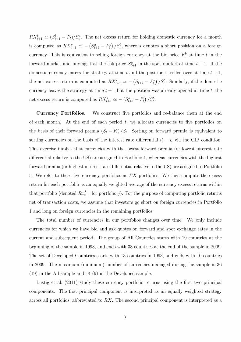
Currency Portfolios. We construct five portfolios and re-balance them at the end

of each month. At the end of each period t, we allocate currencies to five portfolios on

the basis of their forward premia (St − Ft) /St. Sorting on forward premia is equivalent to

sorting currencies on the basis of the interest rate differential i∗t − it via the CIP condition.

This exercise implies that currencies with the lowest forward premia (or lowest interest rate

differential relative to the US) are assigned to Portfolio 1, whereas currencies with the highest

forward premia (or highest interest rate differential relative to the US) are assigned to Portfolio

5. We refer to these five currency portfolios as FX portfolios. We then compute the excess

return for each portfolio as an equally weighted average of the currency excess returns within

that portfolio (denoted Rxjt+1 for portfolio j). For the purpose of computing portfolio returns

net of transaction costs, we assume that investors go short on foreign currencies in Portfolio

1 and long on foreign currencies in the remaining portfolios.

The total number of currencies in our portfolios changes over time. We only include

currencies for which we have bid and ask quotes on forward and spot exchange rates in the

current and subsequent period. The group of All Countries starts with 19 countries at the

beginning of the sample in 1993, and ends with 33 countries at the end of the sample in 2009.

The set of Developed Countries starts with 13 countries in 1993, and ends with 10 countries

in 2009. The maximum (minimum) number of currencies managed during the sample is 36

(19) in the All sample and 14 (9) in the Developed sample.

Lustig et al. (2011) study these currency portfolio returns using the first two principal

components. The first principal component is interpreted as an equally weighted strategy

across all portfolios, abbreviated to RX. The second principal component is interpreted as a

7

strategy with a long position in Portfolio 5 and a short position in Portfolio 1. This is the carry

trade strategy that borrows in the money markets of low yielding currencies and invests in the

money markets of high yielding currencies (note that by construction it is dollar-neutral in a

sense that %-level change in all USD/FCU bilateral rates does not affect the return on high-

minus-low strategy). This high-minus-low portfolio is called the slope factor, and is denoted

as HMLFX .

Table 3 presents summary statistics for the five currency portfolios. The first panel displays

the results for All Countries, while the second panel refers to Developed Countries. All

numbers are annualized. Average excess returns display an increasing pattern when moving

from Portfolio 1 to Portfolio 5 for both samples. The annualized average excess return on

Portfolio 1 is about −2.30 percent per annum for All Countries, and −2.09 percent per annum

for Developed Countries. Portfolio 5 exhibits an annualized average excess return of 8.82

percent per annum for All Countries, and 5.57 percent per annum for Developed Countries.

The average excess return from holding an equally weighted portfolio of foreign currencies

(RX portfolio) is 2.21 percent per annum for All Countries, and 1.60 percent per annum

for Developed Countries. These figures, taken together, suggest that a US investor would

demand a low but positive risk premium for holding foreign currency while borrowing in the

US money market. The average excess return from a long-short strategy that borrows in

low-interest rate currencies and invests in high-interest rate currencies (HMLFX portfolio) is

around 11.12 percent per annum for All Countries and 7.65 percent per annum for Developed

Countries. We find skewness of opposite signs for low- and high-interest portfolios, consistent

with the findings of Brunnermeier et al. (2009) who suggest that investment currencies (or

high yielding currencies) may be subject to ‘crash’ risk.

The realized Sharpe ratio (SR) is equal to the average excess return of a portfolio divided by

the standard deviation of the portfolio returns. The SR simply measures the excess return per

unit of volatility. The SR increases systematically when moving from Portfolio 1 to Portfolio

5. For instance, the annualized SR for All Countries ranges from −0.34 (Portfolio 1) to

0.99 (Portfolio 5). The results are largely comparable for Developed Countries. Finally, we

report the portfolios’ turnover (turn), computed as the ratio between the number of portfolio

switches and the total number of currencies at each date: overall, there is little variation in

8

the composition of these portfolios, which is not surprising given that interest rates are known

to be very persistent.

Shocks to Disagreement about Macro Variables. Dispersion in beliefs measure

for each country and for each macro variable is constructed using cross-sectional standard

deviation with fixed horizon transformation as in Buraschi and Whelan (2012). For instance,

for CA top 3 average (bottom 3 average and consensus are done in the same fashion) fixed

horizon forecast is constructed as follows:

CAf,FHTOP

t+k = (1− k/12)× CAf,SRTOP

t+k + (k/12)× CAf,LRTOP

t+k

where k is the number of the months in the current year, SR and LR are short and long

horizon forecasts respectively (both available at t+ k), and the macro forecasts enter in gross

percentage change format. The disagreement proxy used in our framework is:

DiB(CA) =√

log 2× (logCAf,FHTOP

t+k − logCAf,FHBOTTOM

t+k ) (1)

The following reasoning for such proxy is provided. Due to forecast data limitations discussed

above we are restricted to think about e.g. top 3 average forecast as being a forecast provided

by a relatively optimistic agent and vice versa for the bottom 3 average forecast - it is regarded

as a point estimate of a relatively pessimistic agent. Then DiB(x) can be seen as a scaled

analogue of Parkinson (1980)’s measure for volatility13:

STD(x) =

√1

4 log 2× (log xFHTOP − log xFHBOTTOM ) (2)

Information on the properties of individual country macro time series constructed above is

available upon request.

13Qualitatively the empirical results are unchanged if one uses the ‘simpler’ dispersion measure:

logCAf,FHTOP

t+k − logCAf,FHBOTTOM

t+k . Such measure is also consistent with MAD measure of Beber et al.

(2010):

MAD(x) = 1/2× ((| log xFHTOP − log xFHCONSENSUS |)+ (| log xFHBOTTOM − log xFHCONSENSUS |))= 1/2× (log xFHTOP − log xFHBOTTOM )

9

The aggregate disagreement, which we term MAD, for each macro variable is then calcu-

lated as the cross sectional average14. Note that variables are highly persistent with first lag

autocorrelation ranging from 0.73 to 0.87 (Table 1) largely because of overlapping forecast

horizon. First principal component explains roughly 70% of the data. The figure plots of the

time series are available upon request.

Due to high persistence of aggregate MADs of five macro variables mentioned above, it

was decided, consistent with Menkhoff et al. (2012) and Mancini et al. (2012), to fit univariate

AR(p)-type process with a constant and two lags (i.e. p = 2), based on Box-Jenkins statistic,

and take the residuals. The resulting innovations to MADs are then used in the asset pricing

tests15. The descriptive statistics are displayed in Table 2. Two things are worth paying

attention to. Firstly, shocks by construction do not display any persistence in univariate

analysis. Thus one can interpret innovations as unexpected shocks. Secondly, shocks to

current account disagreement correlate the least with other shocks, indicating ∆DiBCA could

contain extra information potentially missing in other macro disagreement measures.

In addition, we construct a tradeable factor analogue. Following Balduzzi and Robotti

(2008) and Menkhoff et al. (2012), we regress innovations to MADs one at a time on the

currency portfolios described above adding a constant. Coefficients (ex-constant) are then

used as weights forming a factor-mimicking portfolio. We denote corresponding traded factors

as ∆DiBfactor.

As it was mentioned earlier, the exact date when forecasts were made is hard to pin down.

This is a natural constraint which authors cannot do much about. Hence, as a robustness

check, it was decided to perform asset pricing tests assuming various forecast collection dates.

The parameter was varied from the last business day of the previous month to the last business

day before or equal to the 25th day of the current month of the issue. The results are available

upon request. In general, significant coefficients survive within the reasonable distance (6-7

days) of the 1st date of the month used in default setting.

14Correlation with first principal component is above 0.96, but at at the same time having advantage of

not using forward-looking information. Furthermore, the empirical results are robust to using cross sectional

standard deviation of individual disagreement proxies instead.15Fitting AR(12) instead did not change any of the empirical conclusions

10

3 Asset pricing tests

This section presents the cross-sectional asset pricing tests between the five currency portfolios

and macro disagreement shocks, and empirically documents that the returns to carry trades

can be thought of as compensation for risk.

Methods. Consistent with standard empirical asset pricing literature we make the

following two main assumptions. Firstly, there is no arbitrage, and, hence – since carry

portfolios constructed to be zero-cost – risk-adjusted returns for each portfolio should be zero:

Et[Rxjt+1Mt+1] = 0 (3)

for some existing SDF Mt. Secondly, SDF is affine in factors. In particular, the base case

specification assumes the following form where Φ contains two factors - RX and ∆DiB16:

Mt = 1− (Φt − µΦ)′b (4)

where µΦ represents unconditional factor means and b’s are also known as factor loadings.

This specification (3)-(4) implies beta-pricing model:

E[Rxjt ] = λ′βj (5)

where βj contains quantities of risk of portfolio j (measured through covariance with the risk

factors) and λ’s contain the corresponding prices

βj ≡ V −1Φ cov(Rxjt ,Φt)

λ ≡ VΦb

In this paper the empirical unconditional asset pricing tests are performed only (i.e. in-

strument set contains only a constant). At most two families of tests are employed - cross

sectional (XS) and time series (TS). The former is performed under the generalized method

of moments (GMM) methodology. It is inherited from the reviewed empirical asset pricing

16Apart from Lustig et al. (2011) who invent it, RX was also used in the SDFs of Menkhoff et al. (2012)

and Burnside (2011a) to control for the level.

11

works to estimate factor loadings b’s in (4) and λ’s as well as their standard errors (com-

puted with the help of Hansen (1982), Burnside (2007), and Burnside (2011b)). Long run

variance-covariance matrix of the sample moments is estimated with Newey and West (1987)

and optimal number of lags according to Andrews (1991). Alternative XS test is performed

using Fama and MacBeth (1973) procedure with betas estimated over the entire time sample

and, again, prices of risk received as main output17. The point estimates are set equal to those

of GMM and the standard errors are calculated either similarly with Newey and West (1987)

or with Shanken (1992). In the tables below the cross-sectional R2 and the p-value of the

χ2 test for the null hypothesis of zero pricing errors are also reported. TS test on the other

hand is the standard application of Cochrane (2005). The reader is referred to Appendix B

for more details on test methodology.

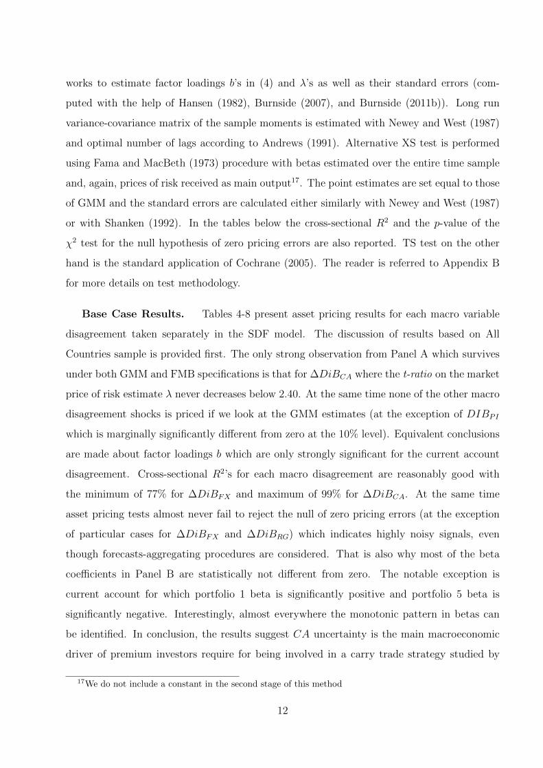
Base Case Results. Tables 4-8 present asset pricing results for each macro variable

disagreement taken separately in the SDF model. The discussion of results based on All

Countries sample is provided first. The only strong observation from Panel A which survives

under both GMM and FMB specifications is that for ∆DiBCA where the t-ratio on the market

price of risk estimate λ never decreases below 2.40. At the same time none of the other macro

disagreement shocks is priced if we look at the GMM estimates (at the exception of DIBPI

which is marginally significantly different from zero at the 10% level). Equivalent conclusions

are made about factor loadings b which are only strongly significant for the current account

disagreement. Cross-sectional R2’s for each macro disagreement are reasonably good with

the minimum of 77% for ∆DiBFX and maximum of 99% for ∆DiBCA. At the same time

asset pricing tests almost never fail to reject the null of zero pricing errors (at the exception

of particular cases for ∆DiBFX and ∆DiBRG) which indicates highly noisy signals, even

though forecasts-aggregating procedures are considered. That is also why most of the beta

coefficients in Panel B are statistically not different from zero. The notable exception is

current account for which portfolio 1 beta is significantly positive and portfolio 5 beta is

significantly negative. Interestingly, almost everywhere the monotonic pattern in betas can

be identified. In conclusion, the results suggest CA uncertainty is the main macroeconomic

driver of premium investors require for being involved in a carry trade strategy studied by

17We do not include a constant in the second stage of this method

12

Lustig et al. (2011) - the result we also establish and verify in numerous exercises below.

Turning to the Developed Countries subsample which is included in the analysis to be

consistent with previous literature (Lustig et al. (2011) and Menkhoff et al. (2012)) one can

notice from Panel A that none of the disagreement shocks are priced if one looks at the GMM

standard errors18. Only ∆DiBIR survives if FMB-based asset pricing test is performed. All

factor loadings are insignificant. On the other hand, again, all cross-sectional R2’s are high and

none of the pricing tests rejects the null. Panel B betas are all not significantly different from

zero (at the exception of portfolio 1 beta on ∆DiBIR), but the monotonic patterns remain for

each shock series. To make any decisive conclusions on Developed Countries sample it would

be preferable to have longer time-series which are unfortunately unavailable to the authors.

Principal Component Decomposition. To make sure all five shocks to aggregate

disagreements are not just noisy proxies on a single risk factor (also keeping in mind from the

base case exercise that all market price estimates were negative, all XS R2’s were comparable,

and portfolio betas displayed monotonic patterns) it is intuitive to dig a bit deeper and perform

principal component analysis on the shocks. In unreported results it turns out that all shocks

load positively on the first principal component (PC1) which is to be expected. Looking

at the Appendix Table C.6 one can notice that indeed PC1 could potentially represent an

important risk factor explaining carry portfolio returns if one looks at monotonic pattern in

betas of Panel B. However, none of the betas is significantly different from zero, as is the case

for market prices and factor loadings in Panel A. Therefore, there is weak evidence that all of

the disagreement shocks are noisy proxies on a single variable.

Furthermore, if one now looks at the disagreement shocks subtracting PC1 effect (i.e.

shock components containing effects of PC2-PC5) one can notice that results on the ∆DiBCA

still hold strongly for All Countries test assets - t-ratio on the market price of risk and factor

loading of current account disagreement shock is way above 2 while betas of extreme portfolios

are significant with opposite intuitive signs consistent with results above. The market price of

risk for ∆DiBFX ex-PC1 becomes significant with unintuitive positive sign and is therefore

disregarded. Finally, ∆DiBPI loses its marginal significance in the previous setting with betas

18In unreported results we find that ∆DiBCA prices ‘Developing Countries’ subsample, defined as All

Countries sample with Developed Countries excluded. Since developing countries constitute the bulk of our

sample it can be concluded that these are responsible for good performance of ∆DiBCA in total cross-section

of countries.

13

now not even making the monotonic pattern and each not being statistically different from

zero.

Factor-mimicking portfolio. Becoming convinced that current account forecasts

contain most relevant information in our setting and to conserve space, Table 9 reports the

asset pricing results only for ∆DiBCA. First, looking at Panel A - market price of risk

and loading on CA factor are significant. Now that the ∆DiBCA is theoretically traded an

additional restriction is that factor mean is statistically indistinguishable from its risk price.

This is satisfied - as we can see the mean of 0.72 is contained within one standard error

band from λCA estimate independent on whether we use GMM or FMB procedure. R2 by

construction is identical to that of Table 4 and XS asset pricing test does not reject the null19.

Now, moving to Panel B - all betas apart from portfolio 3 are significantly different from zero

with becoming familiar monotonic pattern. The time series asset pricing test, consistently

with cross sectional one, does not reject the null of zero pricing errors. Therefore, additional

support for importance of current account-linked factor is provided.

Horse races. Table 10 provides horse race analysis in an asset pricing setting among

HMLFX of Lustig et al. (2011), V OLFX of Menkhoff et al. (2012), and our ∆DiBCA. Panel

A starts off by comparing the former and the latter. It should be noted straight away that

our factor is put in a weaker position as high-minus-low portfolio is linear combination of

the test assets and is very likely to be less noisy than the forecast information authors have

at hand. Not very surprising the orthogonalized component of ∆DiBCA with respect to

HMLFX (denoted by ∆DiB⊥CA) does not provide any superior information - bCA loading is

not statistically different from zero. What is more interesting is that orthogonalized HML⊥FX

has insignificant loading while loading on ∆DiBCA has t-ratio comfortably above 2 (as well

as significant risk price).

Panel B continues by comparing V OLFX to ∆DiBCA. Both of the factors are non-tradable.

∆DiB⊥CA does not have significant loading but neither does V OL⊥FX . Interestingly, in both

sets of tests b’s and λ’s maintain the same intuitive sign for ∆DiBCA while switching the sign

for V OLFX .

Finally, in Panel C we also compare the factor-mimicking portfolios V OLFX and ∆DiBCA.

19∆DiBFX fails strongly cross-sectional asset pricing test even at 1% significance level under both GMM

and FMB specification while ∆DiBRG fails marginally under FMB procedure and 10% significance level.

14

Factor loading of ∆DiB⊥CA is significant (it is not so for V OLFX), and reversing the exercise -

b on V OL⊥FX is highly insignificant while it is so for ∆DiBCA, which also has significant price

of risk. To conclude, if anything, neither of the previously studied factors can comfortably

cover information incorporated in ∆DiBCA.

Beta-sorted portfolios. Consistent with previous literature (Lustig et al. (2011)

and Menkhoff et al. (2012)), it is interesting to find out whether investors are demanding

compensation for exchange rate risk. Table 11 presents descriptive statistics of five currency

portfolios sorted monthly on time t−1 estimate of rolling beta of those portfolios with respect

to ∆DiBCA. Rolling period is taken to be 12 months. The first portfolio (P1) contains

currencies with the highest βCA while the last portfolio (P5) contains currencies with the

lowest βCA.

As one can see, from both All Countries and Developed Countries results, the procedure

produces monotonic pattern in mean returns and significant spread between the extreme

portfolios which is captured by HMLβ. Therefore, lower βCA currencies (which generally tend

to correspond to higher interest countries looking at previous tables) earn on average larger

return than higher βCA currencies providing support for risk-based explanation. Noticeably,

both the mean and the Sharpe ratio of HMLβ are half that of HMLFX . This is again

explained by higher noise of forecast data; nevertheless, CA forecasts again prove to be very

informative.

Individual currencies. Next we consider asset pricing exercise with test assets being

switched from portfolios to individual currencies. As currency risk with time can change so

does the demanded risk premium. Therefore, to make sure the same consistent ‘cross-sectional’

carry trade strategy is considered (going long high risk currencies and short low risk ones)

we follow Lustig et al. (2011, p.3753) (in particular, the section which they call ‘Conditional

Risk Premiums’).

Table 12 contains FMB estimation results. As one can notice ∆DiBCA price of risk is

significant and quantitatively similar to that of Table 4 while λRX is as always not significant.

Inherently, strategies on individual currencies contain a lot of noise which is also reflected in

the lower R2 measure relative to that when portfolios are used as test assets.

Additional robustness. Here we briefly describe additional exercises performed to

15

make the proposed case more robust. Firstly, as argued above, in May 1995 there was a

change in the way top and bottom forecasts are reported. Hence, we re-estimated base case

asset pricing tests with May 1995 as the start date for forecast collection. The results are

reported in Tables C.1-C.5 in Appendix. Again, ∆DiBCA on All (and Developed) Countries

is the only one that comfortably survives.

Secondly, wary of the peso events, consistent with Menkhoff et al. (2012) we winsorize

the extreme high values of the ∆DiBCA at 95%-tile and see if it makes any difference. As

Table C.7 suggests peso events cannot be entirely responsible for observed carry portfolio

premia. All the results remain qualitatively unchanged relative to the base case.

Thirdly, we look at exchange rate component of the return - ∆st+1 - of each portfolio.

We find that earlier observed monotonic pattern in portfolio betas is mainly attributed to

sensitivities of the exchange rate component to ∆DiBCA. Hence, consistent with earlier

literature (Lustig et al. (2011) and Menkhoff et al. (2012)) we find support to exchange rate

risk compensation as a source of carry premia. The results are available in Table C.8. Notice,

that again current account disagreement shock is the only factor for which betas on extreme

portfolios are significant with opposite intuitive signs.

Fourthly, we consider a simpled measure of individual differences in beliefs: DiB(factor)simple =

factorTOPt+k − factorBOTTOMt+k from which the aggregate DiB’s and corresponding shocks are

constructed. Table C.9 displays the estimated coefficients. The conclusions are unchanged20.

Finally, instead of separating into developed and developing countries subsamples we split

all countries into those appearing the Blue Chip (BC) database and those that do not (ex-BC).

Test assets are constructed on currencies in these two categories. Tables C.10-C.14 suggest

that DIBCA price of risk is marginally significant at 10% on BC sample and highly significant

on ex-BC sample. Therefore, there is information in forecasts about some currencies which

are relevant for pricing others.

20Separately, in unreported results we also find that aggregate DiB proxy constructed from XS standard

deviation rather XS mean of individual country-month DiB’s indicates once more current account as the only

factor containing relevant information for pricing carry return portfolios. Hence, no matter how we tweak the

procedure CA forecasts remain the informative source of carry trade performance.

16

4 Conclusion

FX traders often describe carry returns as picking up pennies in front of a steam roller.

Most of the time it pays off. But every once in a while, the low-yielding currencies suddenly

appreciate, and investors caught short are squashed. In this paper, we study the risk-return

profile of this strategy that borrows in low interest rate currencies and invests in high interest

rate currencies. If high interest rate currencies deliver low returns during bad times, then

currency excess returns simply compensate investors for higher risk-exposure and carry trade

returns reflect time-varying risk premia (Fama, 1984; Engel, 1996).

Armed with agents’ expectations of future fundamentals and prices, we construct proxies of

macroeconomic disagreement and find that investment currencies deliver low returns whereas

funding currencies offer a hedge when disagreement about the current account is unexpectedly

high. This result suggests that investors demand a currency risk premium for bearing external

adjustment risk via the trade channel, thus suggesting an economically meaningful explanation

of the UIP anomaly in foreign exchange markets.

17

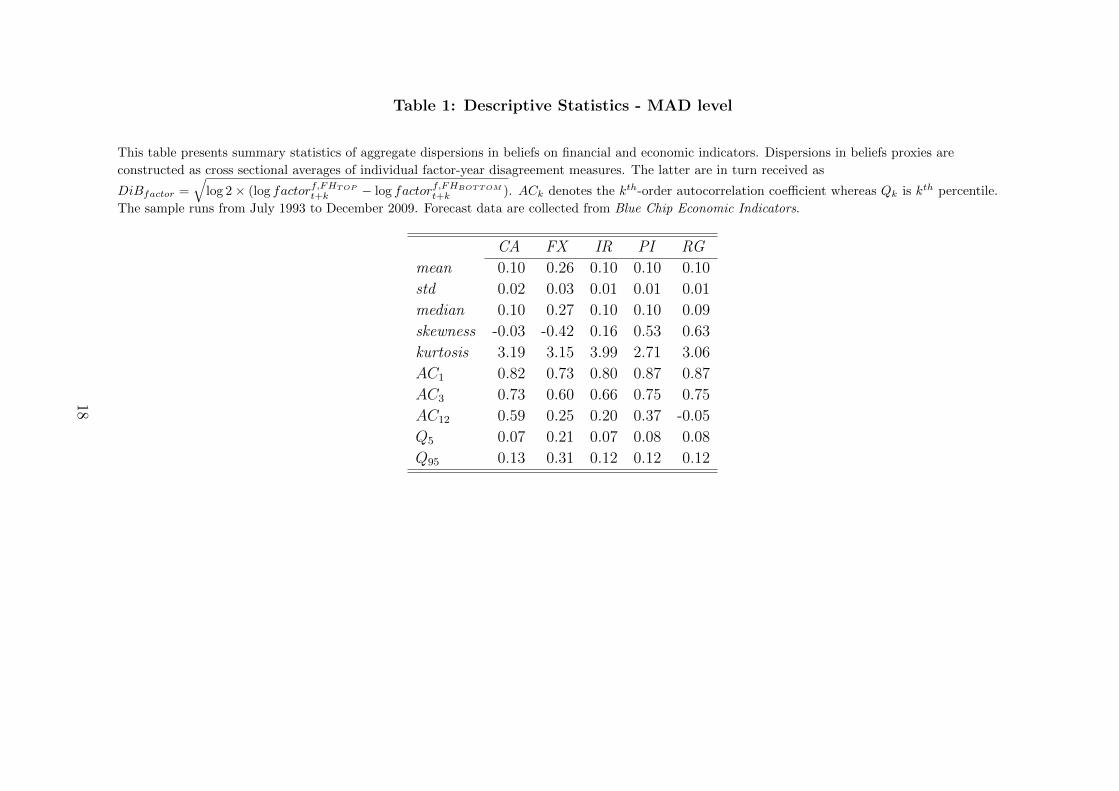
Table 1: Descriptive Statistics - MAD level

This table presents summary statistics of aggregate dispersions in beliefs on financial and economic indicators. Dispersions in beliefs proxies are

constructed as cross sectional averages of individual factor-year disagreement measures. The latter are in turn received as

DiBfactor =√

log 2× (log factorf,FHTOP

t+k − log factorf,FHBOTTOM

t+k ). ACk denotes the kth-order autocorrelation coefficient whereas Qk is kth percentile.

The sample runs from July 1993 to December 2009. Forecast data are collected from Blue Chip Economic Indicators.

CA FX IR PI RG

mean 0.10 0.26 0.10 0.10 0.10

std 0.02 0.03 0.01 0.01 0.01

median 0.10 0.27 0.10 0.10 0.09

skewness -0.03 -0.42 0.16 0.53 0.63

kurtosis 3.19 3.15 3.99 2.71 3.06

AC1 0.82 0.73 0.80 0.87 0.87

AC3 0.73 0.60 0.66 0.75 0.75

AC12 0.59 0.25 0.20 0.37 -0.05

Q5 0.07 0.21 0.07 0.08 0.08

Q95 0.13 0.31 0.12 0.12 0.12

18

Table 2: Descriptive Statistics - MAD innovations

This table presents statistical properties of the innovations to aggregate disagreements fitting an AR(2) process to each of the level series based on

Box-Jenkins statistic. Panel A reports descriptive statistics on individual macro variable time series while Panel B shows the correlation structure among

those. The sample runs from September 1993 to December 2009. Forecast data are collected from Blue Chip Economic Indicators.

Panel A: Individual Series Statistics

CA FX IR PI RG

std 0.01 0.02 0.01 0.01 0.01

skewness -0.23 -0.42 0.03 -0.11 -0.26

kurtosis 4.02 4.37 4.41 4.00 5.46

AC1 -0.06 -0.04 0.02 0.00 -0.01

Panel B: Sample Cross Correlations

CA 1.00

FX 0.27 1.00

IR 0.34 0.43 1.00

PI 0.26 0.41 0.37 1.00

RG 0.20 0.45 0.40 0.58 1.00

19

Table 3: Descriptive Statistics - FX carry portfolios

This table presents descriptive statistics of five currency portfolios sorted monthly on time t− 1 forward premia (nominal interest rate differentials). The

first portfolio (P1) contains currencies with the lowest forward premia while the last portfolio (P5) contains currencies with the highest forward premia.

RX denotes the average across all portfolios. HML is a long-short strategy that buys P5 and sells P1. The table also reports the first order

autocorrelation coefficient (AC1), standard error of the mean (mean SE ) with Newey and West (1987), the annualized Sharpe ratio (Sharpe), and the

portfolios’ turnover (turn). Excess returns are expressed in percentage per annum and adjusted for transaction costs that occur in a short position (P1)

and long position (P2-P5). The sample runs from September 1993 to December 2009. Exchange rates are from Datastream.

Portfolio 1 2 3 4 5 HML RX

All Countries

mean -2.30 -0.45 2.06 2.90 8.82 11.12 2.21

std 6.85 6.76 7.09 7.23 8.93 8.43 6.33

median -0.91 0.77 1.63 4.33 10.53 11.30 4.04

skewness 0.07 -0.23 -0.42 -0.56 -0.22 -0.27 -0.49

kurtosis 4.38 4.00 6.36 7.15 6.70 5.06 5.19

AC1 0.12 0.09 0.22 0.20 0.26 0.20 0.20

mean SE 0.54 0.50 0.63 0.59 0.83 0.72 0.55

Sharpe -0.34 -0.07 0.29 0.40 0.99 1.32 0.35

turn 0.18 0.31 0.32 0.29 0.16

Developed Countries

mean -2.09 0.67 1.82 2.05 5.57 7.65 1.60

std 8.84 9.37 9.12 8.54 10.51 9.98 8.05

median -1.10 1.52 5.43 2.40 5.16 10.24 4.29

skewness 0.08 0.10 -0.17 -0.79 -0.07 -0.92 -0.10

kurtosis 3.22 3.48 4.07 6.82 6.61 6.68 4.13

AC1 0.10 0.09 0.13 0.16 0.09 0.17 0.13

mean SE 0.68 0.71 0.72 0.70 0.80 0.83 0.65

Sharpe -0.24 0.07 0.20 0.24 0.53 0.77 0.20

turn 0.14 0.28 0.32 0.22 0.12

20

Table 4: Asset Pricing - Dispersion in Beliefs on Current Account

This table reports cross-sectional asset pricing results. The linear SDF model includes the average across currency portfolios (RX) and the shock to

aggregate disagreement on the current account changes (∆DiBCA) as factors whereas the test assets are excess returns to five currency portfolios sorted

on the one-month forward premia (nominal interest rate differentials). The first portfolio (P1) contains currencies with the lowest forward premia while

the last portfolio (P5) contains currencies with the highest forward premia. Panel A reports GMM and Fama and MacBeth (1973), FMB, estimates of

the market price of risk λ, the cross-sectional R2 as well as the factor loadings b. Panel B reports least-squares estimates of time series regressions.

Newey and West (1987) standard errors with Andrews (1991) optimal lag selection are reported in parentheses. sh denotes Shanken (1992) standard

errors. pvalχ denotes p-values from the cross-sectional asymptotic asset pricing test for the null hypothesis of zero pricing errors based on χ2-distributed

test statistics. Excess returns are expressed in percentage per annum and adjusted for transaction costs that occur in a short position (P1) and long

position (P2-P5). The portfolios are rebalanced monthly from September 1993 to December 2009. Exchange rates are from Datastream whereas forecast

data are collected from Blue Chip Economic Indicators.

Panel I: Factor Prices and Loadings

All Countries Developed Countries

RX CA R2 pvalχ RX CA R2 pvalχbGMM 0.17 -1.69 99% 96% bGMM 0.16 -1.58 95% 94%

(0.11) (0.66) (0.14) (1.31)

λGMM 0.14 -1.78 λGMM 0.13 -1.67

(0.35) (0.73) (0.35) (1.41)

λFMB 0.14 -1.78 99% λFMB 0.13 -1.67 95%

(0.16) (0.40) 71% (0.16) (0.69) 59%

(sh) (0.13) (0.68) 95% (sh) (0.17) (1.14) 94%

Panel II: Factor Betas

Porfolio α βRX βCA R2 Porfolio α βRX βCA R2

1 -0.51 1.03 0.28 58% 1 -0.30 0.91 0.18 47%

(0.15) (0.15) (0.11) (0.17) (0.17) (0.13)

2 -0.15 0.89 0.12 74% 2 -0.12 1.19 0.07 69%

(0.08) (0.06) (0.07) (0.10) (0.09) (0.09)

3 0.01 0.97 -0.02 80% 3 -0.02 1.22 -0.02 75%

(0.07) (0.06) (0.07) (0.10) (0.07) (0.10)

4 0.10 0.99 -0.08 78% 4 0.01 1.10 -0.06 69%

(0.08) (0.07) (0.07) (0.10) (0.09) (0.09)

5 0.55 1.12 -0.30 63% 5 0.27 1.34 -0.14 67%

(0.13) (0.09) (0.12) (0.13) (0.14) (0.13)

21

Table 5: Asset Pricing - Dispersion in Beliefs on Exchange Rate


aggregate disagreement on the exchange rate changes (∆DiBFX) as factors whereas the test assets are excess returns to five currency portfolios sorted on

the one-month forward premia (nominal interest rate differentials). The first portfolio (P1) contains currencies with the lowest forward premia while the

last portfolio (P5) contains currencies with the highest forward premia. Panel A reports GMM and Fama and MacBeth (1973), FMB, estimates of the

market price of risk λ, the cross-sectional R2 as well as the factor loadings b. Panel B reports least-squares estimates of time series regressions. Newey

and West (1987) standard errors with Andrews (1991) optimal lag selection are reported in parentheses. sh denotes Shanken (1992) standard errors.

pvalχ denotes p-values from the cross-sectional asymptotic asset pricing test for the null hypothesis of zero pricing errors based on χ2-distributed test

statistics. Excess returns are expressed in percentage per annum and adjusted for transaction costs that occur in a short position (P1) and long position

(P2-P5). The portfolios are rebalanced monthly from September 1993 to December 2009. Exchange rates are from Datastream whereas forecast data are

collected from Blue Chip Economic Indicators.



RX FX R2 pvalχ RX FX R2 pvalχbGMM 0.07 -1.69 77% 72% bGMM 0.06 -0.77 90% 92%

(0.23) (1.48) (0.13) (0.85)

λGMM 0.14 -6.70 λGMM 0.16 -3.05

(1.00) (5.92) (0.52) (3.38)

λFMB 0.14 -6.70 77% λFMB 0.16 -3.05 90%

(0.16) (1.49) 1% (0.16) (1.24) 55%

(sh) (0.13) (4.56) 74% (sh) (0.17) (1.90) 89%


Porfolio α βRX βFX R2 Porfolio α βRX βFX R2

1 -0.52 1.05 0.05 57% 1 -0.31 0.93 0.12 47%

(0.15) (0.16) (0.06) (0.16) (0.17) (0.09)

2 -0.15 0.90 0.04 74% 2 -0.12 1.20 0.02 68%

(0.08) (0.06) (0.04) (0.10) (0.09) (0.05)

3 0.01 0.97 0.02 80% 3 -0.02 1.22 -0.01 75%

(0.07) (0.06) (0.04) (0.10) (0.07) (0.05)

4 0.10 0.98 -0.05 78% 4 0.01 1.09 0.02 69%

(0.08) (0.07) (0.04) (0.10) (0.09) (0.06)

5 0.55 1.10 -0.06 62% 5 0.27 1.33 -0.05 67%

(0.13) (0.09) (0.07) (0.13) (0.14) (0.09)

22

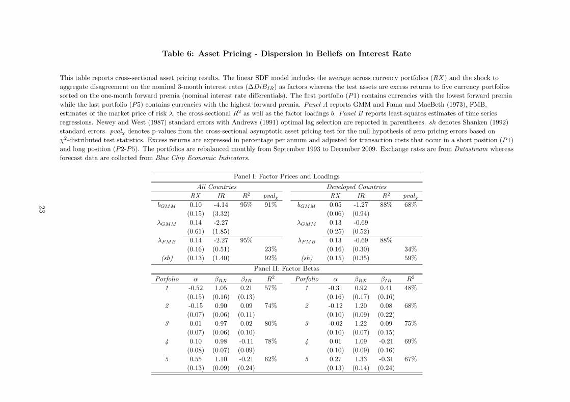
Table 6: Asset Pricing - Dispersion in Beliefs on Interest Rate


aggregate disagreement on the nominal 3-month interest rates (∆DiBIR) as factors whereas the test assets are excess returns to five currency portfolios

sorted on the one-month forward premia (nominal interest rate differentials). The first portfolio (P1) contains currencies with the lowest forward premia

while the last portfolio (P5) contains currencies with the highest forward premia. Panel A reports GMM and Fama and MacBeth (1973), FMB,

estimates of the market price of risk λ, the cross-sectional R2 as well as the factor loadings b. Panel B reports least-squares estimates of time series

regressions. Newey and West (1987) standard errors with Andrews (1991) optimal lag selection are reported in parentheses. sh denotes Shanken (1992)

standard errors. pvalχ denotes p-values from the cross-sectional asymptotic asset pricing test for the null hypothesis of zero pricing errors based on

χ2-distributed test statistics. Excess returns are expressed in percentage per annum and adjusted for transaction costs that occur in a short position (P1)

and long position (P2-P5). The portfolios are rebalanced monthly from September 1993 to December 2009. Exchange rates are from Datastream whereas

forecast data are collected from Blue Chip Economic Indicators.



RX IR R2 pvalχ RX IR R2 pvalχbGMM 0.10 -4.14 95% 91% bGMM 0.05 -1.27 88% 68%

(0.15) (3.32) (0.06) (0.94)

λGMM 0.14 -2.27 λGMM 0.13 -0.69

(0.61) (1.85) (0.25) (0.52)

λFMB 0.14 -2.27 95% λFMB 0.13 -0.69 88%

(0.16) (0.51) 23% (0.16) (0.30) 34%

(sh) (0.13) (1.40) 92% (sh) (0.15) (0.35) 59%


Porfolio α βRX βIR R2 Porfolio α βRX βIR R2

1 -0.52 1.05 0.21 57% 1 -0.31 0.92 0.41 48%

(0.15) (0.16) (0.13) (0.16) (0.17) (0.16)

2 -0.15 0.90 0.09 74% 2 -0.12 1.20 0.08 68%

(0.07) (0.06) (0.11) (0.10) (0.09) (0.22)

3 0.01 0.97 0.02 80% 3 -0.02 1.22 0.09 75%

(0.07) (0.06) (0.10) (0.10) (0.07) (0.15)

4 0.10 0.98 -0.11 78% 4 0.01 1.09 -0.21 69%

(0.08) (0.07) (0.09) (0.10) (0.09) (0.16)

5 0.55 1.10 -0.21 62% 5 0.27 1.33 -0.31 67%

(0.13) (0.09) (0.24) (0.13) (0.14) (0.24)

23

Table 7: Asset Pricing - Dispersion in Beliefs on Inflation Rate


aggregate disagreement on the inflation rates (∆DiBPI) as factors whereas the test assets are excess returns to five currency portfolios sorted on the

one-month forward premia (nominal interest rate differentials). The first portfolio (P1) contains currencies with the lowest forward premia while the last

portfolio (P5) contains currencies with the highest forward premia. Panel A reports GMM and Fama and MacBeth (1973), FMB, estimates of the

market price of risk λ, the cross-sectional R2 as well as the factor loadings b. Panel B reports least-squares estimates of time series regressions. Newey

and West (1987) standard errors with Andrews (1991) optimal lag selection are reported in parentheses. sh denotes Shanken (1992) standard errors.

pvalχ denotes p-values from the cross-sectional asymptotic asset pricing test for the null hypothesis of zero pricing errors based on χ2-distributed test

statistics. Excess returns are expressed in percentage per annum and adjusted for transaction costs that occur in a short position (P1) and long position

(P2-P5). The portfolios are rebalanced monthly from September 1993 to December 2009. Exchange rates are from Datastream whereas forecast data are

collected from Blue Chip Economic Indicators.



RX PI R2 pvalχ RX PI R2 pvalχbGMM 0.08 -4.79 95% 86% bGMM 0.11 -4.11 95% 99%

(0.12) (2.82) (0.14) (4.57)

λGMM 0.14 -1.77 λGMM 0.26 -1.52

(0.54) (1.07) (0.51) (1.70)

λFMB 0.14 -1.77 95% λFMB 0.26 -1.52 95%

(0.16) (0.40) 22% (0.17) (0.62) 77%

(sh) (0.13) (1.03) 92% (sh) (0.23) (1.41) 98%


Porfolio α βRX βPI R2 Porfolio α βRX βPI R2

1 -0.52 1.05 0.24 57% 1 -0.31 0.93 0.30 47%

(0.15) (0.16) (0.15) (0.16) (0.17) (0.21)

2 -0.15 0.90 0.16 74% 2 -0.12 1.20 0.12 69%

(0.07) (0.06) (0.12) (0.09) (0.09) (0.19)

3 0.01 0.97 -0.03 80% 3 -0.02 1.22 0.09 75%

(0.07) (0.06) (0.12) (0.10) (0.07) (0.18)

4 0.10 0.98 -0.07 77% 4 0.01 1.09 0.08 69%

(0.08) (0.07) (0.08) (0.10) (0.09) (0.17)

5 0.55 1.10 -0.31 62% 5 0.27 1.32 -0.04 67%

(0.13) (0.09) (0.20) (0.13) (0.14) (0.22)

24

Table 8: Asset Pricing - Dispersion in Beliefs on Real Growth


aggregate disagreement on the real GDP growth rates (∆DiBRG) as factors whereas the test assets are excess returns to five currency portfolios sorted


the last portfolio (P5) contains currencies with the highest forward premia. Panel A reports GMM and Fama and MacBeth (1973), FMB, estimates of

the market price of risk λ, the cross-sectional R2 as well as the factor loadings b. Panel B reports least-squares estimates of time series regressions.

Newey and West (1987) standard errors with Andrews (1991) optimal lag selection are reported in parentheses. sh denotes Shanken (1992) standard

errors. pvalχ denotes p-values from the cross-sectional asymptotic asset pricing test for the null hypothesis of zero pricing errors based on χ2-distributed

test statistics. Excess returns are expressed in percentage per annum and adjusted for transaction costs that occur in a short position (P1) and long

position (P2-P5). The portfolios are rebalanced monthly from September 1993 to December 2009. Exchange rates are from Datastream whereas forecast

data are collected from Blue Chip Economic Indicators.



RX RG R2 pvalχ RX RG R2 pvalχbGMM -0.08 -5.56 93% 89% bGMM 0.01 -2.23 78% 58%

(0.14) (4.78) (0.09) (2.51)

λGMM 0.15 -2.24 λGMM 0.20 -0.90

(0.91) (1.96) (0.46) (1.02)

λFMB 0.15 -2.24 93% λFMB 0.20 -0.90 78%

(0.16) (0.51) 10% (0.17) (0.41) 14%

(sh) (0.13) (1.58) 91% (sh) (0.17) (0.61) 61%


Porfolio α βRX βRG R2 Porfolio α βRX βRG R2

1 -0.52 1.05 0.24 57% 1 -0.31 0.94 0.37 47%

(0.15) (0.16) (0.21) (0.16) (0.16) (0.27)

2 -0.15 0.90 -0.02 74% 2 -0.12 1.20 0.19 69%

(0.08) (0.06) (0.11) (0.09) (0.09) (0.15)

3 0.01 0.97 0.03 80% 3 -0.02 1.22 0.11 75%

(0.07) (0.06) (0.11) (0.10) (0.07) (0.14)

4 0.10 0.98 -0.02 77% 4 0.01 1.09 -0.12 69%

(0.08) (0.07) (0.10) (0.10) (0.09) (0.15)

5 0.55 1.09 -0.23 62% 5 0.27 1.32 -0.07 67%

(0.13) (0.08) (0.20) (0.13) (0.14) (0.21)

25

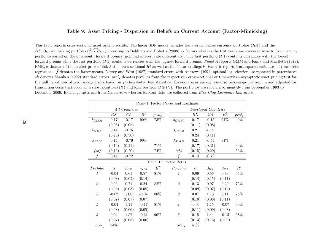
Table 9: Asset Pricing - Dispersion in Beliefs on Current Account (Factor-Mimicking)

This table reports cross-sectional asset pricing results. The linear SDF model includes the average across currency portfolios (RX) and the

∆DiBCA-mimicking portfolio (∆DiBCA) according to Balduzzi and Robotti (2008) as factors whereas the test assets are excess returns to five currency

portfolios sorted on the one-month forward premia (nominal interest rate differentials). The first portfolio (P1) contains currencies with the lowest

forward premia while the last portfolio (P5) contains currencies with the highest forward premia. Panel A reports GMM and Fama and MacBeth (1973),

FMB, estimates of the market price of risk λ, the cross-sectional R2 as well as the factor loadings b. Panel B reports least-squares estimates of time series

regressions. f denotes the factor means. Newey and West (1987) standard errors with Andrews (1991) optimal lag selection are reported in parentheses.

sh denotes Shanken (1992) standard errors. pvalχ denotes p-values from the respective - cross-sectional or time-series - asymptotic asset pricing test for

the null hypothesis of zero pricing errors based on χ2-distributed test statistics. Excess returns are expressed in percentage per annum and adjusted for

transaction costs that occur in a short position (P1) and long position (P2-P5). The portfolios are rebalanced monthly from September 1993 to

December 2009. Exchange rates are from Datastream whereas forecast data are collected from Blue Chip Economic Indicators.




(0.08) (0.05) (0.11) (0.08)

λGMM 0.14 -0.76 λGMM 0.21 -0.59

(0.23) (0.30) (0.24) (0.41)

λFMB 0.14 -0.76 99% λFMB 0.21 -0.59 91%

(0.16) (0.21) 71% (0.17) (0.31) 39%

(sh) (0.13) (0.20) 74% (sh) (0.15) (0.29) 53%

f 0.14 -0.72 f 0.14 -0.72



1 -0.04 0.61 0.57 81% 1 0.09 0.56 0.48 64%

(0.08) (0.05) (0.14) (0.14) (0.15) (0.11)

2 0.06 0.71 0.24 82% 2 0.13 0.97 0.29 75%

(0.06) (0.03) (0.08) (0.09) (0.07) (0.12)

3 -0.02 1.00 -0.04 80% 3 0.07 1.13 0.11 76%

(0.07) (0.07) (0.07) (0.10) (0.06) (0.11)

4 -0.04 1.11 -0.17 81% 4 -0.04 1.15 -0.07 69%

(0.08) (0.06) (0.05) (0.11) (0.09) (0.08)

5 0.04 1.57 -0.61 90% 5 0.15 1.44 -0.15 68%

(0.07) (0.05) (0.06) (0.13) (0.13) (0.09)

pvalχ 94% pvalχ 51%

26

Table 10: Asset Pricing - horse race among ∆DiBCA, HMLFX, and V OLFX

This table reports cross-sectional asset pricing results. As factors the linear SDF model includes the average across currency portfolios (RX) and two of

the three - HMLFX , ∆DiBCA and V OLFX - one of which, denoted by ⊥, is always orthogonalized with respect to the other. For the latter two the

horse race between the corresponding mimicking portfolios, denoted by tilde, is also included. The test assets are excess returns to five currency

portfolios sorted on the one-month forward premia (nominal interest rate differentials). The first portfolio (P1) contains currencies with the lowest

forward premia while the last portfolio (P5) contains currencies with the highest forward premia. The panels report GMM estimates of the factor

loadings b, the market price of risk λ, the cross-sectional R2 as well as p-values from the cross-sectional asymptotic asset pricing test pvalχ. Newey and

West (1987) standard errors with Andrews (1991) optimal lag selection are reported in parentheses. Excess returns are expressed in percentage per

annum and adjusted for transaction costs that occur in a short position (P1) and long position (P2-P5). The portfolios are rebalanced monthly from

September 1993 to December 2009. Exchange rates are from Datastream whereas forecast data are collected from Blue Chip Economic Indicators.

Panel A: ∆DiBCA vs. HMLFX

RX ∆DiB⊥CA HMLFX R2 pvalχ RX ∆DiBCA HML⊥FX R2 pvalχbGMM 0.10 -0.09 0.13 100% 93% bGMM 0.10 -0.14 0.07 100% 93%

(0.11) (0.11) (0.03) (0.12) (0.06) (0.09)

λGMM 0.14 0.04 1.07 λGMM 0.14 -0.73 0.47

(0.22) (0.18) (0.40) (0.23) (0.32) (0.25)

Panel B: ∆DiBCA vs. V OLFX

RX ∆DiB⊥CA V OLFX R2 pvalχ RX ∆DiBCA V OL⊥FX R2 pvalχbGMM 0.30 -2.42 3.81 100% 97% bGMM 0.30 -2.39 5.22 100% 97%

(0.39) (2.36) (14.16) (0.39) (2.29) (15.45)

λGMM 0.14 -2.53 0.02 λGMM 0.14 -2.51 0.04

(0.44) (2.47) (0.12) (0.44) (2.40) (0.13)

Panel C: ∆DiBCA vs. V OLFX

RX ∆DiB⊥CA V OLFX R2 pvalχ RX ∆DiBCA V OL

⊥FX R2 pvalχ

bGMM 0.19 -0.18 -0.054 99% 59% bGMM 0.19 -0.18 0.01 99% 61%

(0.12) (0.09) (0.034) (0.12) (0.06) (0.05)

λGMM 0.14 -0.35 -1.15 λGMM 0.14 -0.76 -0.70

(0.24) (0.25) (0.50) (0.25) (0.29) (0.45)

27

Table 11: Portfolios Sorted on βCA

This table presents descriptive statistics of five currency portfolios sorted monthly on time t− 1 estimate of rolling beta of those portfolios with respect to

∆DiBCA. The first portfolio (P1) contains currencies with the highest βCA while the last portfolio (P5) contains currencies with the lowest βCA. HML

is a long-short strategy that buys P5 and sells P1. The table also reports the first order autocorrelation coefficient (AC1), standard error of the mean

(mean SE ) with Newey and West (1987), the annualized Sharpe ratio (Sharpe), and the portfolios’ turnover (turn). Excess returns are expressed in

percentage per annum and adjusted for transaction costs that occur in a short position (P1) and long position (P2-P5). The sample runs from

September 1994 to December 2009. Exchange rates are from Datastream.

Portfolio 1 2 3 4 5 HMLβAll Countries

mean -0.04 0.07 2.45 2.25 3.55 3.59

std 11.15 7.41 6.39 6.82 10.50 11.84

median 2.42 2.30 1.49 1.29 5.51 1.07

skewness -0.55 -0.55 0.02 -0.01 -0.81 -0.02

kurtosis 4.59 5.76 5.34 6.20 6.83 4.79

AC1 0.25 0.04 0.18 0.11 0.42 0.31

mean SE 1.05 0.55 0.52 0.53 1.15 1.00

Sharpe 0.00 0.01 0.38 0.33 0.34 0.30

turn 0.23 0.42 0.44 0.41 0.22

Developed Countries

mean -0.23 0.58 1.41 1.80 4.34 4.56

std 10.04 10.26 8.63 9.67 9.11 8.80

median 1.18 1.10 3.40 3.01 2.37 5.75

skewness 0.23 0.28 0.08 -0.20 -0.84 -0.24

kurtosis 4.53 3.88 3.62 5.23 6.41 3.80

AC1 -0.01 0.06 0.10 0.18 0.11 0.01

mean SE 0.73 0.78 0.68 0.85 0.71 0.65

Sharpe -0.02 0.06 0.16 0.19 0.48 0.52

turn 0.26 0.45 0.45 0.38 0.24

28

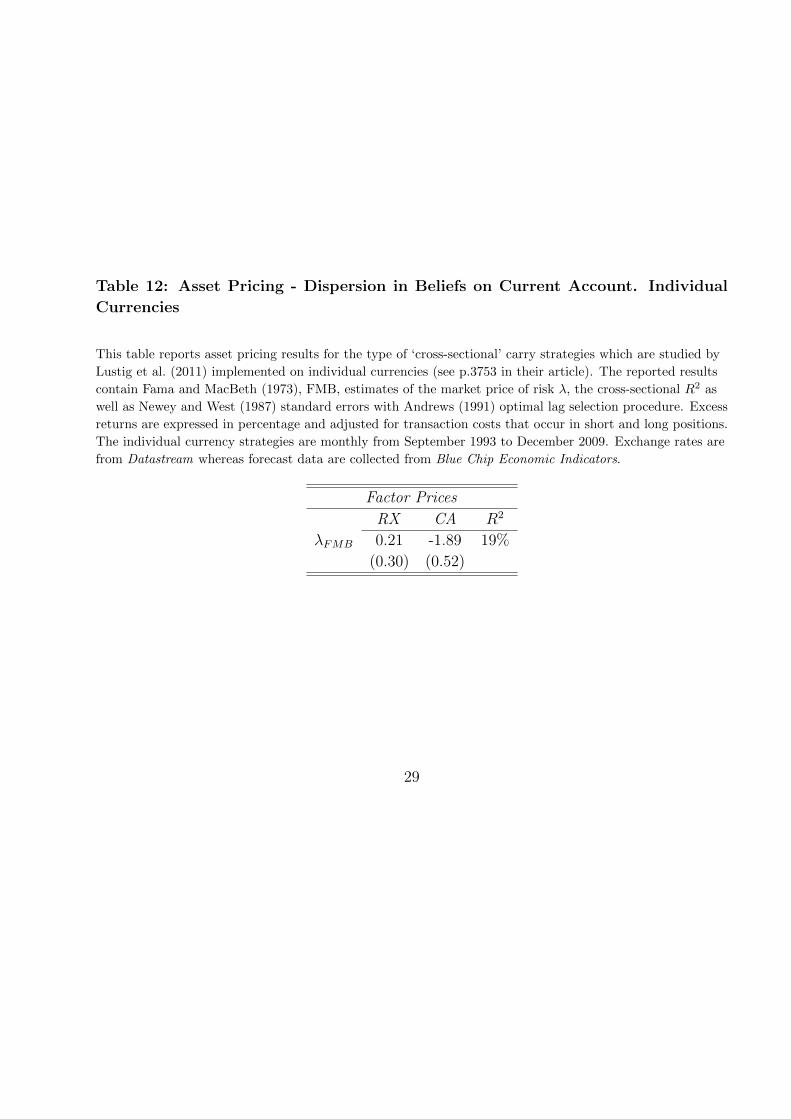
Table 12: Asset Pricing - Dispersion in Beliefs on Current Account. Individual

Currencies

This table reports asset pricing results for the type of ‘cross-sectional’ carry strategies which are studied by

Lustig et al. (2011) implemented on individual currencies (see p.3753 in their article). The reported results

contain Fama and MacBeth (1973), FMB, estimates of the market price of risk λ, the cross-sectional R2 as

well as Newey and West (1987) standard errors with Andrews (1991) optimal lag selection procedure. Excess

returns are expressed in percentage and adjusted for transaction costs that occur in short and long positions.

The individual currency strategies are monthly from September 1993 to December 2009. Exchange rates are

from Datastream whereas forecast data are collected from Blue Chip Economic Indicators.

Factor Prices

RX CA R2

λFMB 0.21 -1.89 19%

(0.30) (0.52)

29

Figure 1: The figure plots the shocks to MADCA versus return on the HMLFX of Lustig et al. (2011)

30

References

E. W. Anderson, E. Ghysels, and J. L. Juergens. Do heterogeneous beliefs matter for assetpricing? Review of Financial Studies, 18(3):875–924, 2005. doi: 10.1093/rfs/hhi026. URLhttp://rfs.oxfordjournals.org/content/18/3/875.abstract.

E. W. Anderson, E. Ghysels, and J. L. Juergens. The impact of risk and uncertaintyon expected returns. Journal of Financial Economics, 94(2):233 – 263, 2009. ISSN0304-405X. doi: 10.1016/j.jfineco.2008.11.001. URL http://www.sciencedirect.com/science/article/pii/S0304405X09001275.

D. W. K. Andrews. Heteroskedasticity and autocorrelation consistent covariance matrix esti-mation. Econometrica, 59(3):pp. 817–858, 1991. ISSN 00129682. URL http://www.jstor.org/stable/2938229.

P. Balduzzi and C. Robotti. Mimicking portfolios, economic risk premia, and tests of multi-beta models. Journal of Business & Economic Statistics, 26(3):354–368, 2008. doi:10.1198/073500108000000042. URL http://www.tandfonline.com/doi/abs/10.1198/073500108000000042.

A. Beber, F. Breedon, and A. Buraschi. Differences in beliefs and currency risk premiums.Journal of Financial Economics, 98:415–438, 2010.

M. K. Brunnermeier, S. Nagel, and L. H. Pedersen. Carry Trades and Currency Crashes,chapter 5, pages 313–347. University of Chicago Press, 2009.

A. Buraschi and P. Whelan. Term structure models with differences in beliefs. working paper,2012. URL http://ssrn.com/abstract=1887644.

C. Burnside. Empirical asset pricing and statistical power in the presence of weak risk factors.appendix. working paper, 2007. URL http://www.duke.edu/~acb8/research.htm.

C. Burnside. The cross section of foreign currency risk premia and consumption growth risk:Comment. American Economic Review, 101(7):3456–76, December 2011a. doi: 10.1257/aer.101.7.3456. URL http://www.aeaweb.org/articles.php?doi=10.1257/aer.101.7.3456.

C. Burnside. Online appendix to the cross section of foreign currency risk premia andconsumption growth risk: Comment. American Economic Review, December 2011b.doi: 10.1257/aer.101.7.3456. URL http://www.aeaweb.org/articles.php?doi=10.1257/aer.101.7.3456.

J. H. Cochrane. Asset Pricing. Princeton University Press, revised edition, 2005.

C. Engel and K. D. West. Global interest rates, currency returns, and the real value of thedollar. American Economic Review, 100(2):562–67, 2010. doi: 10.1257/aer.100.2.562. URLhttp://www.aeaweb.org/articles.php?doi=10.1257/aer.100.2.562.

E. F. Fama and J. D. MacBeth. Risk, return, and equilibrium: Empirical tests. Journal ofPolitical Economy, 81(3):pp. 607–636, 1973. ISSN 00223808. URL http://www.jstor.org/stable/1831028.

P. Gourinchas and H. Rey. International financial adjustment. Journal of Political Economy,115(4):pp. 665–703, 2007. ISSN 00223808. URL http://www.jstor.org/stable/10.1086/521966.

31

http://rfs.oxfordjournals.org/content/18/3/875.abstract

http://www.sciencedirect.com/science/article/pii/S0304405X09001275

http://www.sciencedirect.com/science/article/pii/S0304405X09001275

http://www.jstor.org/stable/2938229


http://www.tandfonline.com/doi/abs/10.1198/073500108000000042

http://www.tandfonline.com/doi/abs/10.1198/073500108000000042

http://ssrn.com/abstract=1887644

http://www.duke.edu/~acb8/research.htm

http://www.aeaweb.org/articles.php?doi=10.1257/aer.101.7.3456







http://www.jstor.org/stable/10.1086/521966

http://www.jstor.org/stable/10.1086/521966

P.-O. Gourinchas. Valuation effects and external adjustment: a review. Current Account andExternal Financing, XII:195–236, 2008.

J. D. Hamilton. Times Series Analysis. Princeton University Press, 1994.

L. P. Hansen. Large sample properties of generalized method of moments estimators. Econo-metrica, 50(4):pp. 1029–1054, 1982. ISSN 00129682. URL http://www.jstor.org/stable/1912775.

M. S. Kim and F. Zapatero. Competitive compensation and dispersion in analysts’ recommen-dations. working paper, 2011. URL http://marshallinside.usc.edu/zapatero/Papers/analyst%20recommendation%20game%20Aug%202011.pdf.

H. Lustig, N. Roussanov, and A. Verdelhan. Common risk factors in currency markets. Reviewof Financial Studies, 24(11):3731–3777, 2011. doi: 10.1093/rfs/hhr068. URL http://rfs.oxfordjournals.org/content/24/11/3731.abstract.

L. Mancini, A. Ranaldo, and J. Wrampelmeyer. Liquidity in the foreign exchange market:Measurement, commonality, and risk premiums. The Journal of Finance, forthcoming,2012.

L. Menkhoff, L. Sarno, M. Schmeling, and A. Schrimpf. Carry trades and global foreignexchange volatility. The Journal of Finance, forthcoming, 2012.

W. K. Newey and K. D. West. A simple, positive semi-definite, heteroskedasticity and au-tocorrelation consistent covariance matrix. Econometrica, 55(3):pp. 703–708, 1987. ISSN00129682. URL http://www.jstor.org/stable/1913610.

M. Parkinson. The extreme value method for estimating the variance of the rate of return.The Journal of Business, 53(1):pp. 61–65, 1980. ISSN 00219398. URL http://www.jstor.org/stable/2352357.

L. Sarno and M. Schmeling. Which fundamentals drive exchange rates? a cross-sectionalperspective. Journal of Money, Credit and Banking, forthcoming, 2012.

J. Shanken. On the estimation of beta-pricing models. Review of Financial Studies, 5(1):1–55, 1992. doi: 10.1093/rfs/5.1.1. URL http://rfs.oxfordjournals.org/content/5/1/1.abstract.

32



http://marshallinside.usc.edu/zapatero/Papers/analyst%20recommendation%20game%20Aug%202011.pdf

http://marshallinside.usc.edu/zapatero/Papers/analyst%20recommendation%20game%20Aug%202011.pdf








6 BLUE CHIP ECONOMIC INDICATORS JANUARY 10, 2013

BLUE CHIP INTERNATIONAL CONSENSUS FORECASTS

------------------------------------------ANNUAL DATA---------------------------------------- -------------------------END OF YEAR----------------------------Real Economic Inflation Current Account Exchange Rate Interest

Growth % Change % Change In Billions Against RatesGDP Consumer Prices Of U.S. Dollars U.S. $ 3-Month

CANADA 2013 2014 2013 2014 2013 2014 2013 2014 2013 2014January Consensus 1.9 2.5 1.8 2.1 -60.2 -56.2 1.00 1.02 1.14 1.73 Top 3 Avg. 2.2 3.1 2.0 2.6 -47.2 -40.4 1.03 1.07 1.37 2.15 Bottom 3 Avg. 1.5 2.2 1.6 1.4 -72.3 -70.0 0.96 0.98 0.97 1.30 Last Month Avg. 2.0 na 1.8 na -52.5 na 1.01 na 1.26 na

2011* 2012** 2011* 2012** 2011* 2012** Latest Year Ago Latest Year Ago Actual 2.5 2.1 2.9 1.7 -47.1 -58.4 0.98 1.01 1.24 0.82

MEXICO 2013 2014 2013 2014 2013 2014 2013 2014 2013 2014January Consensus 3.4 4.1 4.0 3.8 -9.3 -11.4 12.69 12.73 4.87 5.49 Top 3 Avg. 3.8 4.9 4.4 4.2 -5.4 -5.5 13.02 13.12 5.32 6.00 Bottom 3 Avg. 2.8 3.5 3.8 3.5 -13.7 -17.7 12.23 12.27 4.47 4.98 Last Month Avg. 3.5 na 3.9 na -10.4 na 12.75 na 4.72 na


JAPAN 2013 2014 2013 2014 2013 2014 2013 2014 2013 2014January Consensus 0.7 1.2 -0.2 0.7 49.9 46.5 84.2 87.0 0.17 0.24 Top 3 Avg. 1.5 1.8 0.1 1.8 79.3 81.8 90.3 93.6 0.27 0.40 Bottom 3 Avg. 0.2 0.7 -0.5 -0.2 23.6 13.8 79.5 80.8 0.08 0.08 Last Month Avg. 0.8 na -0.3 na 65.1 na 83.6 na 0.15 na

2011* 2012** 2011* 2012** 2011* 2012** Latest Year Ago Latest Year Ago Actual -0.7 1.8 -0.3 0.0 130.3 65.0 87.2 76.7 0.17 0.15

UNITED KINGDOM 2013 2014 2013 2014 2013 2014 2013 2014 2013 2014January Consensus 1.0 1.7 2.5 2.1 -76.8 -66.7 1.58 1.58 0.52 0.81 Top 3 Avg. 1.3 2.2 2.9 2.6 -58.9 -48.8 1.62 1.66 0.66 1.07 Bottom 3 Avg. 0.4 1.1 2.1 1.7 -92.9 -86.2 1.53 1.49 0.37 0.51 Last Month Avg. 1.2 na 2.4 na -61.5 na 1.56 na 0.58 na

2011* 2012** 2011* 2012** 2011* 2012** Latest Year Ago Latest Year Ago Actual 0.7 -0.1 4.5 2.8 -19.8 -79.3 1.64 1.56 0.50 1.10

SOUTH KOREA 2013 2014 2013 2014 2013 2014 2013 2014 2013 2014January Consensus 3.1 4.0 2.5 2.9 32.7 29.3 1080 1052 3.10 4.28 Top 3 Avg. 3.6 4.9 2.9 3.3 42.6 43.6 1110 1096 3.46 5.12 Bottom 3 Avg. 2.4 3.1 2.0 2.5 24.1 17.7 1043 1011 2.81 3.54 Last Month Avg. 3.1 na 2.6 na 23.7 na 1069 na 3.18 na

2011* 2012** 2011* 2012** 2011* 2012** Latest Year Ago Latest Year Ago Actual 3.6 2.3 4.0 2.3 23.2 31.4 1064 1149 2.87 3.56

GERMANY 2013 2014 2013 2014 2013 2014 2013 2014 2013 2014January Consensus 0.9 1.4 1.9 1.9 188.3 186.9 1.26 1.24 0.41 0.70 Top 3 Avg. 1.4 2.1 2.2 2.2 210.4 208.1 1.31 1.29 0.76 0.98 Bottom 3 Avg. 0.6 0.5 1.7 1.7 166.3 165.7 1.19 1.20 0.21 0.35 Last Month Avg. 1.0 na 1.8 na 179.6 na 1.24 na 0.46 na

2011* 2012** 2011* 2012** 2011* 2012** Latest Year Ago Latest Year Ago Actual 3.1 0.9 2.3 2.1 176.1 196.4 1.32 1.30 0.19 1.32

TAIWAN 2013 2014 2013 2014 2013 2014 2013 2014 2013 2014January Consensus 3.1 4.1 1.6 1.9 42.4 42.8 29.29 29.21 1.10 1.37 Top 3 Avg. 3.8 4.9 1.9 2.3 45.2 46.1 30.49 30.34 1.33 1.56 Bottom 3 Avg. 2.2 3.3 1.4 1.5 39.4 39.1 28.40 28.51 0.91 1.20 Last Month Avg. 3.1 na 1.8 na 39.8 na 29.35 na 1.06 na


NETHERLANDS 2013 2014 2013 2014 2013 2014 2013 2014 2013 2014January Consensus -0.2 0.9 2.4 1.9 53.9 56.1 1.26 1.24 0.41 0.70 Top 3 Avg. 0.7 1.7 2.6 2.4 59.7 61.8 1.31 1.29 0.76 0.98 Bottom 3 Avg. -0.8 0.1 2.1 1.4 46.9 50.2 1.19 1.20 0.21 0.35 Last Month Avg. 0.1 na 2.3 na 52.1 na 1.24 na 0.46 na

2011* 2012** 2011* 2012** 2011* 2012** Latest Year Ago Latest Year Ago Actual 1.3 -0.8 2.3 2.5 58.3 56.9 1.32 1.30 0.19 1.32

1

*Best estimates available. **In most all cases, actual data for 2012 GDP, consumer prices and current account are not yet available. Where it is unavailable, figures are consensus forecasts from December 10, 2012 Blue Chip Economic Indicators. Figures are currency units per U.S. dollar except for U.K., Australia and the Euro.

JANUARY 10, 2013 BLUE CHIP ECONOMIC INDICATORS 7

BLUE CHIP INTERNATIONAL CONSENSUS FORECASTS

------------------------------------------ANNUAL DATA---------------------------------------- ------------------------END OF YEAR----------------------------Real Economic Inflation Current Account Exchange Rate Interest

Growth % Change % Change In Billions Against RatesGDP Consumer Prices Of U.S. Dollars U.S. $ 3-Month

RUSSIA 2013 2014 2013 2014 2013 2014 2013 2014 2013 2014January Consensus 3.4 3.9 6.3 5.9 64.5 45.9 31.1 31.5 6.72 6.52 Top 3 Avg. 3.9 4.3 7.0 7.2 84.7 65.7 31.7 32.6 8.25 7.75 Bottom 3 Avg. 3.1 3.5 5.5 5.1 45.1 29.0 30.5 30.3 5.00 5.29 Last Month Avg. 3.6 na 6.4 na 55.2 na 31.4 na 7.22 na


FRANCE 2013 2014 2013 2014 2013 2014 2013 2014 2013 2014January Consensus 0.2 1.0 1.7 1.6 -46.7 -40.6 1.26 1.24 0.41 0.70 Top 3 Avg. 0.6 1.5 2.1 2.0 -42.5 -33.8 1.31 1.29 0.76 0.98 Bottom 3 Avg. -0.1 0.1 1.3 0.9 -50.9 -47.4 1.19 1.20 0.21 0.35 Last Month Avg. 0.3 na 1.7 na -44.4 na 1.24 na 0.46 na


BRAZIL 2013 2014 2013 2014 2013 2014 2013 2014 2013 2014January Consensus 3.4 4.1 5.7 5.5 -54.8 -54.4 2.02 2.00 7.57 8.74 Top 3 Avg. 4.3 5.1 6.1 6.2 -45.5 -44.1 2.11 2.12 7.86 9.48 Bottom 3 Avg. 2.1 3.4 5.2 5.1 -65.5 -66.2 1.94 1.89 7.29 8.00 Last Month Avg. 3.8 na 5.5 na -56.4 na 2.01 na 7.93 na


HONG KONG 2013 2014 2013 2014 2013 2014 2013 2014 2013 2014January Consensus 3.2 4.1 4.0 3.8 11.0 13.1 7.77 7.77 0.34 0.35 Top 3 Avg. 4.1 5.0 4.8 4.3 14.0 15.9 7.80 7.79 0.49 0.50 Bottom 3 Avg. 2.2 3.3 3.1 3.4 8.0 10.7 7.75 7.76 0.17 0.19 Last Month Avg. 3.5 na 3.9 na 9.7 na 7.76 na 0.40 na


INDIA 2013 2014 2013 2014 2013 2014 2013 2014 2013 2014January Consensus 6.0 7.0 7.6 6.7 -67.2 -63.4 52.8 51.7 8.08 8.04 Top 3 Avg. 6.6 7.8 8.5 8.0 -52.2 -42.7 54.5 53.9 9.24 8.77 Bottom 3 Avg. 5.1 6.1 6.8 5.0 -80.0 -83.1 51.2 49.3 7.23 7.38 Last Month Avg. 6.2 na 7.7 na -68.3 na 53.0 na 8.10 na


CHINA 2013 2014 2013 2014 2013 2014 2013 2014 2013 2014January Consensus 8.0 8.1 3.1 3.6 242.2 224.3 6.22 6.12 4.71 4.98 Top 3 Avg. 8.3 8.6 3.9 4.0 282.3 297.7 6.33 6.22 5.58 5.96 Bottom 3 Avg. 7.8 7.6 2.6 3.1 199.3 140.6 6.12 6.00 3.83 4.00 Last Month Avg. 8.0 na 3.1 na 242.7 na 6.19 na 4.83 na


AUSTRALIA 2013 2014 2013 2014 2013 2014 2013 2014 2013 2014January Consensus 2.7 3.1 2.7 2.7 -87.3 -86.2 1.01 1.00 3.05 3.58 Top 3 Avg. 3.3 3.6 3.1 3.1 -58.7 -60.0 1.06 1.07 3.41 4.05 Bottom 3 Avg. 2.2 2.5 2.1 2.3 -124.2 -117.0 0.93 0.94 2.73 3.13 Last Month Avg. 2.8 na 2.8 na -70.9 na 1.00 na 3.32 na


EUROZONE 2013 2014 2013 2014 2013 2014 2013 2014 2013 2014January Consensus 0.0 0.9 2.0 1.8 127.4 153.8 1.26 1.24 0.41 0.70 Top 3 Avg. 0.4 1.7 2.3 2.0 191.0 225.9 1.31 1.29 0.76 0.98 Bottom 3 Avg. -0.4 -0.2 1.7 1.6 63.9 80.2 1.19 1.20 0.21 0.35 Last Month Avg. 0.1 na 2.0 na 134.3 na 1.24 na 0.46 na

2011* 2012** 2011* 2012** 2011* 2012** Latest Year Ago Latest Year Ago Actual 1.5 -0.4 2.7 2.5 10.3 108.5 1.32 1.30 0.19 1.32

1

Contributors to Blue Chip International Survey: IHS Global Insight, US; Federal Express Corporation, USA; Credit Suisse, US; JP Morgan, US; Economist Intelligence Unit, UK; BMO Capital Markets, Canada; UBS, US; AIG, New York, NY; Oxford Economics, US; Citigroup U.S. Economics; Societe Generale, New York, NY; Bank of America-Merrill Lynch, US; Nomura Capital Markets America, US; Morgan Stanley; US; Moody’s Capital Markets, US; Wells Fargo & Company, US; Moody’s Analyt-ics, US; Swisse Re, U.S.; Barclays Capital, US; General Motors Corp., US; Wintrust Wealth Management, US; and Grupo de Economistas y Asociados, Mexico.

Appendices

A Example of forecasts extract

Source: Aspen Publishers website, http://www.aspenpublishers.com/%5CAspenUI%5CSampleIssuesPDF%5C968.pdf

33

http://www.aspenpublishers.com/%5CAspenUI%5CSampleIssuesPDF%5C968.pdf

B Methodology

B.1 Cross-sectional test

The cross-sectional test could slightly vary from specifications known to authors, and, thus,described below in more detail. The corresponding moment conditions estimated are:

E[RxjtMt] = 0 (6)

E[Φt] = µΦ (7)

vech[E[(Φt − µΦ)(Φt − µΦ)′]] = vech[VΦ] (8)

and 1 ≤ j ≤ n goes through each and every portfolio. Hence, in total we have n + k + lmoment conditions, where k is the number of risk factors and l = k(k + 1)/2 is the numberof non-repeating elements of covariance matrix of factors. Such specification (as in Burnside(2007) and Burnside (2011b)) also implicitly assumes factors are independent over time, and,hence factor covariance matrix is estimated as its simple sample analogue. One could extendby e.g. pre-setting GMM estimator be equal to that of Newey and West (1987).

Summing up, the vector h(.) takes the following form:

h(zt, θ) =

Rxt[1− (Φt − µΦ)′b]

Φt − µΦ

vech[(Φt − µΦ)(Φt − µΦ)′]− vech[VΦ]

(9)

where

z′t =[Rx′t Φ′t

]θ′ =

[b′ µ′Φ vech[VΦ]′

]and g(.) are the sample moment conditions:

g(ZT , θ) =1

T

T∑t=1

h(zt, θ) ≡ ET [h(zt, θ)] (10)

whereZ ′T =

{z′1 z′2 ... z′T

}For joint estimation of first and second moments one can e.g. refer to Burnside (2007) and

Burnside (2011b) whose methodology is followed in this article as well. VΦ is estimated aspart of GMM procedure in order not to underrate standard error of the price of risk λ. Forparameter estimation the following linear combinations of moments (g) summarized in matrixa is set to zero:

aT =

d′1W 0 0

0 Ik 0

0 0 Il

(11)

with d1 = ET [Rxt(Φt−µΦ)′]. Such structure ensures that parameters specifying both first andsecond moments of factors are set equal to their sample analogues. Estimates of b’s can betaken as first or as second stage GMM estimates when considering only moments for pricing

34

equations in isolation (first n rows of g) depending on the choice of W (‘OLS case’ of W = In×nwas assumed throughout).

dT ≡∂g(ZT , θ)

∂θ′

∣∣∣∣θ=θGMM

=

−d1 ET [Rxt]b′GMM 0

0 −Ik 0

0 0 −Il

(12)

The asymptotic covariance matrix of g

S =∞∑

j=−∞

E[h(zt, θ)h(zt−j, θ)′] (13)

is estimated consistently using Newey and West (1987) with optimal number of lags criterionaccording to Andrews (1991). It is assumed throughout the paper that covariance betweenfactor second sample moments and other sample moments is zero.

The joint test for the pricing errors equal to zero is then performed via Cochrane (2005,eq. (11.6)) statistic which is χ2(n− k)-distributed.

Now from definition of λ in (5):

CT ≡∂λ(θ)

∂θ′


=[VΦ 0k×k P

](14)

where

P =∂λ(θ)

∂(vech[VΦ])′

=

b1 b2 b3 · · · bk 0 0 · · · 0 · · · 0 0 0

0 b1 0 · · · 0 b2 b3 · · · bk · · · 0 0 0

0 0 b1 · · · 0 0 b2 · · · 0 · · · 0 0 0...

. . ....

0 0 0 · · · 0 0 0 · · · 0 · · · bk−1 bk 0

0 0 0 · · · b1 0 0 · · · b2 · · · 0 bk−1 bk

Hansen (1982) showed: √

T (θGMM − θ)d−→ N(0, Vθ) (15)

whereVθ = (ad)−1aSa′(d′a′)−1 (16)

Using delta method21: √T (λGMM − λ)

d−→ N(0, CVθC′) (17)

The diagonal elements of the covariance matrix then help to decide whether particular factoris priced or not.

21See e.g. Hamilton (1994, p.214)

35

B.2 Time-series test

Time-series asset pricing test is a standard application of Cochrane (2005, ch 12.1). Nonethe-less, it is noted that since one is working with multiple factors (k > 1) one needs to be carefulwith generalisation of the first formula given on p.234 that is admittedly correct for consideredcase k = 1.

However, as soon as one generalizes to multiple factors and introduces the moment vectorconsistent with notation on p.242 (the last equation):

h(zt, θ) =

[Rxt − α− βΦt

(Rxt − α− βΦt)⊗ Φt

](18)

where

z′t =[Rx′t Φ′t

]θ′ =

[α′ vec[β]′

]then the resulting ‘score’ matrix must have the respective form:

dT ≡∂g(ZT , θ)

∂θ′


= −

[In ET [Φ(1)]In ET [Φ(2)]In · · · ET [Φ(k)]In

In ⊗ ET [Φ] In ⊗Q(:,1)Φ In ⊗Q(:,2)

Φ · · · In ⊗Q(:,k)Φ

]

where Φ(i) denotes the ith element, QΦ = ET [ΦΦ′], and Q(:,i)Φ denotes the ith column. This, for

instance, shows that the first formula on top of p.243 is actually not entirely true given theusual definition of the Kronecker product. The formula for dT right above is the one used intime-series asset pricing test of this paper.

36

C Additional analysis

Table C.1: Asset Pricing - Dispersion in Beliefs on Current Account. May 1995 as start dateThis table reports cross-sectional asset pricing results. The linear SDF model includes the average across currency portfolios (RX) and the shock to



the last portfolio (P5) contains currencies with the highest forward premia. Panel A reports GMM estimates of the factor loadings b, the market price of

risk λ, the cross-sectional R2 as well as p-values from the cross-sectional asymptotic asset pricing test pvalχ. Panel B reports least-squares estimates of

time series regressions. Newey and West (1987) standard errors with Andrews (1991) optimal lag selection are reported in parentheses. Excess returns

are expressed in percentage per annum and adjusted for transaction costs that occur in a short position (P1) and long position (P2-P5). The portfolios

are rebalanced monthly from July 1995 to December 2009. Exchange rates are from Datastream whereas forecast data are collected from Blue Chip

Economic Indicators.


All Countries Developed Countries Developing Countries

RX CA R2 pvalχ RX CA R2 pvalχ RX CA R2 pvalχbGMM 0.12 -1.76 96% 78% bGMM 0.12 -1.98 74% 78% bGMM 0.11 -1.64 62% 27%

(0.10) (0.67) (0.17) (1.92) (0.09) (0.54)

λGMM 0.08 -2.27 λGMM 0.04 -2.56 λGMM 0.08 -2.12

(0.43) (0.92) (0.51) (2.51) (0.40) (0.76)


Porfolio α βRX βCA R2 Porfolio α βRX βCA R2 Porfolio α βRX βCA R2

1 -0.58 1.02 0.20 57% 1 -0.35 0.88 0.04 45% 1 -0.50 0.97 0.19 33%

(0.16) (0.16) (0.08) (0.17) (0.17) (0.14) (0.23) (0.25) (0.08)

2 -0.17 0.89 0.13 76% 2 -0.16 1.18 0.10 70% 2 -0.14 0.60 0.14 60%

(0.08) (0.06) (0.06) (0.09) (0.09) (0.09) (0.08) (0.04) (0.06)

3 0.02 0.95 0.01 80% 3 -0.03 1.20 -0.01 75% 3 0.00 0.83 0.03 74%

(0.07) (0.07) (0.06) (0.11) (0.07) (0.09) (0.08) (0.06) (0.06)

4 0.09 0.99 -0.03 79% 4 -0.03 1.10 -0.02 70% 4 -0.08 1.12 -0.20 64%

(0.08) (0.07) (0.07) (0.10) (0.09) (0.07) (0.13) (0.09) (0.11)

5 0.64 1.14 -0.30 65% 5 0.32 1.36 -0.13 69% 5 0.96 1.11 -0.26 42%

(0.14) (0.09) (0.10) (0.15) (0.14) (0.13) (0.21) (0.13) (0.16)

37

Table C.2: Asset Pricing - Dispersion in Beliefs on Exchange Rate. May 1995 as start date




last portfolio (P5) contains currencies with the highest forward premia. Panel A reports GMM estimates of the factor loadings b, the market price of risk

λ, the cross-sectional R2 as well as p-values from the cross-sectional asymptotic asset pricing test pvalχ. Panel B reports least-squares estimates of time

series regressions. Newey and West (1987) standard errors with Andrews (1991) optimal lag selection are reported in parentheses. Excess returns are

expressed in percentage per annum and adjusted for transaction costs that occur in a short position (P1) and long position (P2-P5). The portfolios are

rebalanced monthly from July 1995 to December 2009. Exchange rates are from Datastream whereas forecast data are collected from Blue Chip




RX FX R2 pvalχ RX FX R2 pvalχ RX FX R2 pvalχbGMM -0.01 -1.98 89% 95% bGMM 0.02 -0.68 92% 93% bGMM 0.00 -1.90 28% 76%

(0.25) (2.04) (0.11) (0.55) (0.25) (2.92)

λGMM 0.08 -12.31 λGMM 0.11 -4.21 λGMM 0.11 -11.80

(1.39) (12.81) (0.53) (3.51) (1.39) (18.25)


Porfolio α βRX βFX R2 Porfolio α βRX βFX R2 Porfolio α βRX βFX R2

1 -0.58 1.03 0.03 56% 1 -0.35 0.89 0.08 46% 1 -0.50 0.98 0.02 33%

(0.16) (0.16) (0.04) (0.17) (0.16) (0.08) (0.25) (0.26) (0.04)

2 -0.17 0.90 0.02 75% 2 -0.16 1.18 0.05 70% 2 -0.14 0.61 0.00 59%

(0.08) (0.06) (0.03) (0.09) (0.09) (0.04) (0.07) (0.05) (0.02)

3 0.02 0.95 0.02 80% 3 -0.03 1.20 -0.02 75% 3 0.00 0.84 0.01 74%

(0.07) (0.07) (0.03) (0.11) (0.07) (0.05) (0.08) (0.07) (0.03)

4 0.09 0.99 -0.02 79% 4 -0.03 1.10 0.03 70% 4 -0.08 1.11 -0.03 63%

(0.08) (0.07) (0.04) (0.10) (0.09) (0.05) (0.13) (0.09) (0.09)

5 0.64 1.12 -0.05 64% 5 0.32 1.35 -0.06 69% 5 0.97 1.09 -0.02 42%

(0.14) (0.09) (0.05) (0.15) (0.14) (0.06) (0.23) (0.13) (0.08)

38

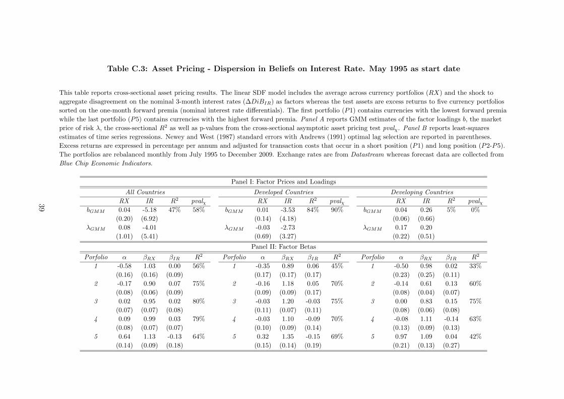
Table C.3: Asset Pricing - Dispersion in Beliefs on Interest Rate. May 1995 as start date




while the last portfolio (P5) contains currencies with the highest forward premia. Panel A reports GMM estimates of the factor loadings b, the market

price of risk λ, the cross-sectional R2 as well as p-values from the cross-sectional asymptotic asset pricing test pvalχ. Panel B reports least-squares

estimates of time series regressions. Newey and West (1987) standard errors with Andrews (1991) optimal lag selection are reported in parentheses.

Excess returns are expressed in percentage per annum and adjusted for transaction costs that occur in a short position (P1) and long position (P2-P5).

The portfolios are rebalanced monthly from July 1995 to December 2009. Exchange rates are from Datastream whereas forecast data are collected from

Blue Chip Economic Indicators.



RX IR R2 pvalχ RX IR R2 pvalχ RX IR R2 pvalχbGMM 0.04 -5.18 47% 58% bGMM 0.01 -3.53 84% 90% bGMM 0.04 0.26 5% 0%

(0.20) (6.92) (0.14) (4.18) (0.06) (0.66)

λGMM 0.08 -4.01 λGMM -0.03 -2.73 λGMM 0.17 0.20

(1.01) (5.41) (0.69) (3.27) (0.22) (0.51)


Porfolio α βRX βIR R2 Porfolio α βRX βIR R2 Porfolio α βRX βIR R2

1 -0.58 1.03 0.00 56% 1 -0.35 0.89 0.06 45% 1 -0.50 0.98 0.02 33%

(0.16) (0.16) (0.09) (0.17) (0.17) (0.17) (0.23) (0.25) (0.11)

2 -0.17 0.90 0.07 75% 2 -0.16 1.18 0.05 70% 2 -0.14 0.61 0.13 60%

(0.08) (0.06) (0.09) (0.09) (0.09) (0.17) (0.08) (0.04) (0.07)

3 0.02 0.95 0.02 80% 3 -0.03 1.20 -0.03 75% 3 0.00 0.83 0.15 75%

(0.07) (0.07) (0.08) (0.11) (0.07) (0.11) (0.08) (0.06) (0.08)

4 0.09 0.99 0.03 79% 4 -0.03 1.10 -0.09 70% 4 -0.08 1.11 -0.14 63%

(0.08) (0.07) (0.07) (0.10) (0.09) (0.14) (0.13) (0.09) (0.13)

5 0.64 1.13 -0.13 64% 5 0.32 1.35 -0.15 69% 5 0.97 1.09 0.04 42%

(0.14) (0.09) (0.18) (0.15) (0.14) (0.19) (0.21) (0.13) (0.27)

39

Table C.4: Asset Pricing - Dispersion in Beliefs on Inflation Rate. May 1995 as start date




portfolio (P5) contains currencies with the highest forward premia. Panel A reports GMM estimates of the factor loadings b, the market price of risk λ,

the cross-sectional R2 as well as p-values from the cross-sectional asymptotic asset pricing test pvalχ. Panel B reports least-squares estimates of time



rebalanced monthly from July 1995 to December 2009. Exchange rates are from Datastream whereas forecast data are collected from Blue Chip




RX PI R2 pvalχ RX PI R2 pvalχ RX PI R2 pvalχbGMM 0.08 -5.24 60% 53% bGMM -0.01 2.40 10% 34% bGMM 0.10 -5.23 84% 84%

(0.14) (3.71) (0.11) (5.30) (0.16) (3.12)

λGMM 0.08 -2.42 λGMM 0.07 1.11 λGMM 0.19 -2.42

(0.64) (1.77) (0.37) (2.46) (0.68) (1.50)


Porfolio α βRX βPI R2 Porfolio α βRX βPI R2 Porfolio α βRX βPI R2

1 -0.58 1.03 0.05 56% 1 -0.35 0.89 -0.04 45% 1 -0.50 0.98 0.29 33%

(0.16) (0.16) (0.16) (0.17) (0.17) (0.21) (0.23) (0.25) (0.21)

2 -0.17 0.89 0.17 75% 2 -0.16 1.18 -0.01 70% 2 -0.14 0.61 0.13 60%

(0.08) (0.06) (0.12) (0.09) (0.09) (0.20) (0.08) (0.04) (0.08)

3 0.02 0.95 0.04 80% 3 -0.03 1.20 0.00 75% 3 0.00 0.84 0.00 74%

(0.07) (0.07) (0.11) (0.11) (0.07) (0.17) (0.08) (0.06) (0.11)

4 0.09 0.99 -0.07 79% 4 -0.03 1.10 0.07 70% 4 -0.08 1.11 -0.05 63%

(0.08) (0.07) (0.07) (0.10) (0.09) (0.14) (0.13) (0.09) (0.16)

5 0.64 1.13 -0.20 64% 5 0.32 1.35 -0.02 68% 5 0.96 1.10 -0.25 42%

(0.14) (0.09) (0.18) (0.15) (0.14) (0.24) (0.21) (0.13) (0.29)

40

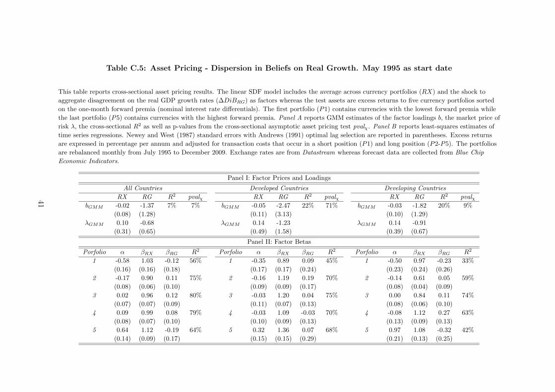
Table C.5: Asset Pricing - Dispersion in Beliefs on Real Growth. May 1995 as start date








are rebalanced monthly from July 1995 to December 2009. Exchange rates are from Datastream whereas forecast data are collected from Blue Chip




RX RG R2 pvalχ RX RG R2 pvalχ RX RG R2 pvalχbGMM -0.02 -1.37 7% 7% bGMM -0.05 -2.47 22% 71% bGMM -0.03 -1.82 20% 9%

(0.08) (1.28) (0.11) (3.13) (0.10) (1.29)

λGMM 0.10 -0.68 λGMM 0.14 -1.23 λGMM 0.14 -0.91

(0.31) (0.65) (0.49) (1.58) (0.39) (0.67)


Porfolio α βRX βRG R2 Porfolio α βRX βRG R2 Porfolio α βRX βRG R2

1 -0.58 1.03 -0.12 56% 1 -0.35 0.89 0.09 45% 1 -0.50 0.97 -0.23 33%

(0.16) (0.16) (0.18) (0.17) (0.17) (0.24) (0.23) (0.24) (0.26)

2 -0.17 0.90 0.11 75% 2 -0.16 1.19 0.19 70% 2 -0.14 0.61 0.05 59%

(0.08) (0.06) (0.10) (0.09) (0.09) (0.17) (0.08) (0.04) (0.09)

3 0.02 0.96 0.12 80% 3 -0.03 1.20 0.04 75% 3 0.00 0.84 0.11 74%

(0.07) (0.07) (0.09) (0.11) (0.07) (0.13) (0.08) (0.06) (0.10)

4 0.09 0.99 0.08 79% 4 -0.03 1.09 -0.03 70% 4 -0.08 1.12 0.27 63%

(0.08) (0.07) (0.10) (0.10) (0.09) (0.13) (0.13) (0.09) (0.13)

5 0.64 1.12 -0.19 64% 5 0.32 1.36 0.07 68% 5 0.97 1.08 -0.32 42%

(0.14) (0.09) (0.17) (0.15) (0.15) (0.29) (0.21) (0.13) (0.25)

41

Table C.6: Asset Pricing - PC1 and Dispersion in Beliefs ex-PC1

This table reports cross-sectional asset pricing results. As factors the linear SDF model includes the average across currency portfolios (RX) and one of

the following - first principal component of the disagreement shocks to five macro variables (PC1) or one of the disagreement shocks with PC1 subtracted

from it. The first portfolio (P1) contains currencies with the lowest forward premia while the last portfolio (P5) contains currencies with the highest

forward premia. Panel A reports GMM estimates of the factor loadings b, the market price of risk λ, the cross-sectional R2 as well as p-values from the

cross-sectional asymptotic asset pricing test pvalχ. Panel B reports least-squares estimates of time series regressions. Newey and West (1987) standard

errors with Andrews (1991) optimal lag selection are reported in parentheses. Excess returns are expressed in percentage per annum and adjusted for

transaction costs that occur in a short position (P1) and long position (P2-P5). The portfolios are rebalanced monthly from September 1993 to December

2009. Exchange rates are from Datastream whereas forecast data are collected from Blue Chip Economic Indicators.

Panel I: Factor Prices and Loadings Panel I: Factor Prices and Loadings Panel I: Factor Prices and Loadings

RX PC1 R2 pvalχ RX CA R2 pvalχ RX FX R2 pvalχbGMM 0.08 -1.36 86% 76% bGMM 0.19 -2.13 99% 97% bGMM 0.12 6.94 99% 98%

(0.21) (1.00) (0.10) (0.83) (0.09) (3.04)

λGMM 0.14 -5.93 λGMM 0.14 -1.93 λGMM 0.14 0.64

(0.85) (4.45) (0.36) (0.79) (0.38) (0.29)

Panel II: Factor Betas Panel II: Factor Betas Panel II: Factor Betas

Porfolio α βRX βPC1 R2 Porfolio α βRX βCA R2 Porfolio α βRX βFX R2

1 -0.52 1.05 0.07 57% 1 -0.51 1.03 0.26 57% 1 -0.52 1.04 -0.82 57%

(0.15) (0.16) (0.06) (0.15) (0.16) (0.10) (0.15) (0.16) (0.31)

2 -0.15 0.90 0.04 74% 2 -0.15 0.89 0.10 74% 2 -0.15 0.90 -0.22 74%

(0.07) (0.06) (0.04) (0.08) (0.06) (0.07) (0.08) (0.06) (0.24)

3 0.01 0.97 0.01 80% 3 0.01 0.97 -0.03 80% 3 0.01 0.97 0.09 80%

(0.07) (0.06) (0.04) (0.07) (0.06) (0.07) (0.07) (0.06) (0.23)

4 0.10 0.98 -0.05 78% 4 0.10 0.99 -0.05 77% 4 0.10 0.98 0.08 77%

(0.08) (0.07) (0.04) (0.08) (0.07) (0.07) (0.08) (0.07) (0.24)

5 0.55 1.10 -0.07 62% 5 0.55 1.12 -0.28 63% 5 0.55 1.11 0.86 63%

(0.13) (0.09) (0.06) (0.13) (0.09) (0.12) (0.13) (0.09) (0.39)

42

Table C.6: (continued)


RX IR R2 pvalχ RX PI R2 pvalχ RX RG R2 pvalχbGMM 0.11 -8.66 99% 100% bGMM 0.07 -8.11 89% 77% bGMM -0.14 -6.68 46% 47%

(0.22) (10.68) (0.14) (5.99) (0.17) (6.58)

λGMM 0.14 -3.50 λGMM 0.14 -2.29 λGMM 0.15 -1.97

(0.96) (4.34) (0.72) (1.72) (0.69) (1.96)


Porfolio α βRX βIR R2 Porfolio α βRX βPI R2 Porfolio α βRX βRG R2

1 -0.52 1.05 0.16 57% 1 -0.52 1.05 0.17 57% 1 -0.52 1.05 0.17 57%

(0.15) (0.16) (0.13) (0.15) (0.16) (0.13) (0.15) (0.16) (0.19)

2 -0.15 0.90 0.03 74% 2 -0.15 0.90 0.12 74% 2 -0.15 0.90 -0.12 74%

(0.08) (0.06) (0.12) (0.07) (0.06) (0.12) (0.08) (0.06) (0.13)

3 0.01 0.97 0.00 80% 3 0.01 0.97 -0.06 80% 3 0.01 0.97 0.01 80%

(0.07) (0.06) (0.10) (0.07) (0.06) (0.11) (0.07) (0.06) (0.10)

4 0.10 0.98 -0.04 77% 4 0.10 0.98 0.01 77% 4 0.10 0.99 0.09 77%

(0.08) (0.07) (0.08) (0.08) (0.07) (0.10) (0.08) (0.07) (0.14)

5 0.55 1.10 -0.14 62% 5 0.55 1.10 -0.24 62% 5 0.55 1.09 -0.14 62%

(0.13) (0.09) (0.27) (0.13) (0.09) (0.20) (0.13) (0.09) (0.21)

43

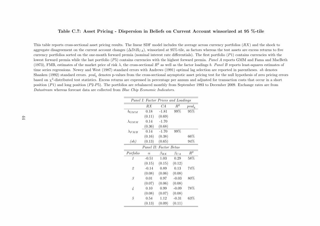
Table C.7: Asset Pricing - Dispersion in Beliefs on Current Account winsorized at 95 %-tile


aggregate disagreement on the current account changes (∆DiBCA), winsorized at 95%-tile, as factors whereas the test assets are excess returns to five

currency portfolios sorted on the one-month forward premia (nominal interest rate differentials). The first portfolio (P1) contains currencies with the

lowest forward premia while the last portfolio (P5) contains currencies with the highest forward premia. Panel A reports GMM and Fama and MacBeth

(1973), FMB, estimates of the market price of risk λ, the cross-sectional R2 as well as the factor loadings b. Panel B reports least-squares estimates of

time series regressions. Newey and West (1987) standard errors with Andrews (1991) optimal lag selection are reported in parentheses. sh denotes

Shanken (1992) standard errors. pvalχ denotes p-values from the cross-sectional asymptotic asset pricing test for the null hypothesis of zero pricing errors

based on χ2-distributed test statistics. Excess returns are expressed in percentage per annum and adjusted for transaction costs that occur in a short

position (P1) and long position (P2-P5). The portfolios are rebalanced monthly from September 1993 to December 2009. Exchange rates are from

Datastream whereas forecast data are collected from Blue Chip Economic Indicators.


RX CA R2 pvalχbGMM 0.18 -1.81 99% 95%

(0.11) (0.69)

λGMM 0.14 -1.70

(0.36) (0.68)

λFMB 0.14 -1.70 99%

(0.16) (0.38) 66%

(sh) (0.13) (0.65) 94%


Porfolio α βRX βCA R2

1 -0.51 1.03 0.29 58%

(0.15) (0.15) (0.12)

2 -0.14 0.89 0.13 74%

(0.08) (0.06) (0.08)

3 0.01 0.97 -0.03 80%

(0.07) (0.06) (0.08)

4 0.10 0.99 -0.09 78%

(0.08) (0.07) (0.08)

5 0.54 1.12 -0.31 63%

(0.13) (0.09) (0.11)

44

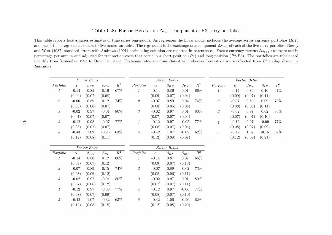
Table C.8: Factor Betas - on ∆st+1 component of FX carry portfolios

This table reports least-squares estimates of time series regressions. As regressors the linear model includes the average across currency portfolios (RX)

and one of the disagreement shocks to five macro variables. The regressand is the exchange rate component ∆st+1 of each of the five carry porfolios. Newey

and West (1987) standard errors with Andrews (1991) optimal lag selection are reported in parentheses. Excess currency returns ∆st+1 are expressed in

percentage per annum and adjusted for transaction costs that occur in a short position (P1) and long position (P2-P5). The portfolios are rebalanced

monthly from September 1993 to December 2009. Exchange rates are from Datastream whereas forecast data are collected from Blue Chip Economic

Indicators.

Factor Betas Factor Betas Factor Betas

Porfolio α βRX βCA R2 Porfolio α βRX βFX R2 Porfolio α βRX βIR R2

1 -0.14 0.85 0.16 67% 1 -0.14 0.86 0.01 66% 1 -0.14 0.86 0.16 67%

(0.09) (0.07) (0.08) (0.09) (0.07) (0.04) (0.09) (0.07) (0.11)

2 -0.06 0.89 0.12 74% 2 -0.07 0.89 0.04 74% 2 -0.07 0.89 0.09 73%

(0.08) (0.06) (0.07) (0.08) (0.05) (0.04) (0.08) (0.06) (0.11)

3 -0.02 0.97 -0.01 80% 3 -0.02 0.97 0.01 80% 3 -0.02 0.97 0.02 80%

(0.07) (0.07) (0.07) (0.07) (0.07) (0.04) (0.07) (0.07) (0.10)

4 -0.12 0.98 -0.07 77% 4 -0.12 0.97 -0.05 77% 4 -0.12 0.97 -0.09 77%

(0.08) (0.07) (0.07) (0.08) (0.07) (0.04) (0.08) (0.07) (0.09)

5 -0.43 1.09 -0.25 63% 5 -0.42 1.07 -0.02 62% 5 -0.42 1.07 -0.15 62%

(0.12) (0.08) (0.11) (0.12) (0.08) (0.07) (0.12) (0.08) (0.21)

Factor Betas Factor Betas

Porfolio α βRX βPI R2 Porfolio α βRX βRG R2

1 -0.14 0.86 0.12 66% 1 -0.14 0.87 0.07 66%

(0.09) (0.07) (0.12) (0.09) (0.07) (0.13)

2 -0.07 0.89 0.15 74% 2 -0.07 0.89 -0.02 73%

(0.08) (0.06) (0.12) (0.08) (0.06) (0.11)

3 -0.02 0.97 -0.04 80% 3 -0.02 0.97 0.01 80%

(0.07) (0.06) (0.12) (0.07) (0.07) (0.11)

4 -0.12 0.97 -0.08 77% 4 -0.12 0.97 -0.06 77%

(0.08) (0.07) (0.09) (0.08) (0.07) (0.10)

5 -0.42 1.07 -0.32 63% 5 -0.42 1.06 -0.26 62%

(0.12) (0.08) (0.18) (0.12) (0.08) (0.20)

45

Table C.9: Asset Pricing - simple Dispersion in Beliefs Measure I

This table reports cross-sectional asset pricing results. As factors the linear SDF model includes the average across currency portfolios (RX) and one of the

disagreement shocks to five macro variables, constructed from simple aggregate disagreement measure: ∆DiB(factor)simple = factorTOPt+k −factorBOTTOMt+k .

The first portfolio (P1) contains currencies with the lowest forward premia while the last portfolio (P5) contains currencies with the highest forward premia.

Panel A reports GMM estimates of the factor loadings b, the market price of risk λ, the cross-sectional R2 as well as p-values from the cross-sectional

asymptotic asset pricing test pvalχ. Panel B reports least-squares estimates of time series regressions. Newey and West (1987) standard errors with

Andrews (1991) optimal lag selection are reported in parentheses. Excess returns are expressed in percentage per annum and adjusted for transaction costs

that occur in a short position (P1) and long position (P2-P5). The portfolios are rebalanced monthly from September 1993 to December 2009. Exchange

rates are from Datastream whereas forecast data are collected from Blue Chip Economic Indicators.


RX CA R2 pvalχ RX FX R2 pvalχ RX IR R2 pvalχbGMM 0.15 -4.95 99% 94% bGMM 0.08 -1.81 86% 80% bGMM 0.06 -7.55 89% 63%

(0.12) (2.44) (0.23) (1.36) (0.10) (4.86)

λGMM 0.14 -0.80 λGMM 0.14 -4.94 λGMM 0.14 -0.67

(0.39) (0.41) (0.97) (3.77) (0.44) (0.45)


Porfolio α βRX βCA R2 Porfolio α βRX βFX R2 Porfolio α βRX βIR R2

1 -0.52 1.03 0.60 57% 1 -0.52 1.05 0.08 57% 1 -0.52 1.05 0.70 57%

(0.15) (0.15) (0.25) (0.15) (0.16) (0.08) (0.15) (0.16) (0.35)

2 -0.15 0.89 0.28 74% 2 -0.15 0.90 0.04 74% 2 -0.15 0.90 0.34 74%

(0.08) (0.06) (0.18) (0.08) (0.06) (0.05) (0.07) (0.06) (0.29)

3 0.01 0.97 -0.04 80% 3 0.01 0.97 0.03 80% 3 0.01 0.97 0.04 80%

(0.07) (0.06) (0.19) (0.07) (0.06) (0.05) (0.07) (0.06) (0.24)

4 0.10 0.99 -0.14 77% 4 0.10 0.98 -0.06 78% 4 0.10 0.98 -0.45 78%

(0.08) (0.07) (0.16) (0.08) (0.07) (0.05) (0.08) (0.07) (0.24)

5 0.55 1.11 -0.69 63% 5 0.55 1.10 -0.09 62% 5 0.55 1.10 -0.62 62%

(0.13) (0.09) (0.35) (0.13) (0.09) (0.07) (0.13) (0.09) (0.56)

46

Table C.9: (continued)

Panel I: Factor Prices and Loadings Panel I: Factor Prices and Loadings

RX PI R2 pvalχ RX RG R2 pvalχbGMM 0.05 -9.83 89% 40% bGMM -0.12 -17.40 93% 89%

(0.09) (5.48) (0.14) (14.24)

λGMM 0.14 -0.53 λGMM 0.15 -0.63

(0.40) (0.31) (0.88) (0.53)

Panel II: Factor Betas Panel II: Factor Betas

Porfolio α βRX βPI R2 Porfolio α βRX βRG R2

1 -0.52 1.05 0.69 57% 1 -0.52 1.06 0.83 57%

(0.15) (0.16) (0.32) (0.15) (0.16) (0.71)

2 -0.15 0.90 0.64 75% 2 -0.15 0.90 -0.04 74%

(0.07) (0.06) (0.31) (0.08) (0.06) (0.38)

3 0.01 0.97 -0.05 80% 3 0.01 0.97 0.13 80%

(0.07) (0.06) (0.27) (0.07) (0.06) (0.38)

4 0.10 0.98 -0.31 78% 4 0.10 0.98 -0.07 77%

(0.08) (0.07) (0.21) (0.08) (0.07) (0.34)

5 0.55 1.10 -0.96 62% 5 0.55 1.09 -0.84 62%

(0.13) (0.09) (0.50) (0.13) (0.08) (0.66)

47

Table C.10: Asset Pricing - Dispersion in Beliefs on Current Account. BC vs. Ex-BC sample








are rebalanced monthly from September 1993 to December 2009. Exchange rates are from Datastream whereas forecast data are collected from Blue Chip



BC Countries Ex-BC Countries


(0.10) (0.79) (0.10) (0.54)

λGMM 0.12 -1.47 λGMM 0.16 -1.72

(0.30) (0.86) (0.35) (0.61)



1 -0.41 0.84 0.27 50% 1 -0.63 1.22 0.36 47%

(0.13) (0.11) (0.11) (0.21) (0.23) (0.18)

2 -0.17 0.74 0.10 54% 2 0.02 0.95 0.13 70%

(0.09) (0.07) (0.09) (0.09) (0.06) (0.09)

3 -0.16 0.81 -0.10 63% 3 0.08 0.97 -0.11 70%

(0.08) (0.06) (0.08) (0.09) (0.08) (0.07)

4 0.07 0.91 0.03 63% 4 -0.02 1.23 -0.12 66%

(0.09) (0.09) (0.10) (0.13) (0.10) (0.14)

5 0.46 0.70 -0.23 35% 5 0.79 1.24 -0.32 48%

(0.15) (0.12) (0.11) (0.21) (0.13) (0.15)

48

Table C.11: Asset Pricing - Dispersion in Beliefs on Exchange Rate. BC vs. Ex-BC sample




last portfolio (P5) contains currencies with the highest forward premia. Panel A reports GMM estimates of the factor loadings b, the market price of risk

λ, the cross-sectional R2 as well as p-values from the cross-sectional asymptotic asset pricing test pvalχ. Panel B reports least-squares estimates of time



rebalanced monthly from September 1993 to December 2009. Exchange rates are from Datastream whereas forecast data are collected from Blue Chip




RX FX R2 pvalχ RX FX R2 pvalχbGMM 0.09 -1.40 86% 90% bGMM 0.06 -1.34 43% 48%

(0.23) (1.35) (0.19) (1.06)

λGMM 0.24 -5.54 λGMM 0.14 -5.31

(0.92) (5.39) (0.80) (4.27)


Porfolio α βRX βFX R2 Porfolio α βRX βFX R2

1 -0.42 0.85 0.08 49% 1 -0.63 1.25 0.06 46%

(0.13) (0.10) (0.07) (0.22) (0.24) (0.09)

2 -0.17 0.75 0.04 54% 2 0.02 0.96 0.06 69%

(0.09) (0.07) (0.04) (0.09) (0.06) (0.05)

3 -0.16 0.80 0.03 63% 3 0.08 0.96 -0.01 70%

(0.08) (0.06) (0.05) (0.09) (0.08) (0.06)

4 0.07 0.91 0.04 63% 4 -0.02 1.22 -0.07 66%

(0.09) (0.10) (0.05) (0.13) (0.09) (0.08)

5 0.47 0.68 -0.08 34% 5 0.79 1.22 -0.06 47%

(0.15) (0.12) (0.07) (0.21) (0.13) (0.11)

49

Table C.12: Asset Pricing - Dispersion in Beliefs on Interest Rate. BC vs. Ex-BC sample




while the last portfolio (P5) contains currencies with the highest forward premia. Panel A reports GMM estimates of the factor loadings b, the market

price of risk λ, the cross-sectional R2 as well as p-values from the cross-sectional asymptotic asset pricing test pvalχ. Panel B reports least-squares

estimates of time series regressions. Newey and West (1987) standard errors with Andrews (1991) optimal lag selection are reported in parentheses.

Excess returns are expressed in percentage per annum and adjusted for transaction costs that occur in a short position (P1) and long position (P2-P5).

The portfolios are rebalanced monthly from September 1993 to December 2009. Exchange rates are from Datastream whereas forecast data are collected

from Blue Chip Economic Indicators.



RX IR R2 pvalχ RX IR R2 pvalχbGMM 0.08 -2.18 90% 79% bGMM 0.07 -1.97 8% 7%

(0.09) (1.17) (0.09) (2.09)

λGMM 0.17 -1.20 λGMM 0.15 -1.08

(0.35) (0.67) (0.33) (1.15)


Porfolio α βRX βIR R2 Porfolio α βRX βIR R2

1 -0.42 0.85 0.42 51% 1 -0.63 1.25 0.07 46%

(0.13) (0.10) (0.14) (0.22) (0.24) (0.20)

2 -0.17 0.75 0.08 54% 2 0.02 0.96 0.14 69%

(0.09) (0.07) (0.16) (0.09) (0.06) (0.14)

3 -0.16 0.80 0.03 63% 3 0.08 0.96 -0.06 70%

(0.08) (0.07) (0.12) (0.09) (0.08) (0.10)

4 0.07 0.91 0.04 63% 4 -0.02 1.22 -0.22 66%

(0.09) (0.09) (0.11) (0.12) (0.09) (0.19)

5 0.46 0.68 -0.33 35% 5 0.79 1.22 -0.06 47%

(0.15) (0.12) (0.17) (0.21) (0.13) (0.31)

50

Table C.13: Asset Pricing - Dispersion in Beliefs on Inflation Rate. BC vs. Ex-BC sample




portfolio (P5) contains currencies with the highest forward premia. Panel A reports GMM estimates of the factor loadings b, the market price of risk λ,

the cross-sectional R2 as well as p-values from the cross-sectional asymptotic asset pricing test pvalχ. Panel B reports least-squares estimates of time



rebalanced monthly from September 1993 to December 2009. Exchange rates are from Datastream whereas forecast data are collected from Blue Chip




RX PI R2 pvalχ RX PI R2 pvalχbGMM 0.07 -3.32 78% 71% bGMM 0.08 -4.80 83% 72%

(0.09) (2.04) (0.13) (2.42)

λGMM 0.15 -1.23 λGMM 0.16 -1.77

(0.38) (0.77) (0.56) (0.92)


Porfolio α βRX βPI R2 Porfolio α βRX βPI R2

1 -0.42 0.85 0.31 50% 1 -0.63 1.25 0.39 46%

(0.13) (0.10) (0.17) (0.22) (0.24) (0.21)

2 -0.17 0.75 0.00 54% 2 0.02 0.96 0.06 69%

(0.09) (0.07) (0.15) (0.09) (0.06) (0.16)

3 -0.16 0.80 0.07 63% 3 0.08 0.96 -0.07 70%

(0.08) (0.07) (0.14) (0.09) (0.08) (0.16)

4 0.07 0.91 0.13 63% 4 -0.02 1.22 -0.16 66%

(0.09) (0.09) (0.19) (0.12) (0.09) (0.17)

5 0.46 0.68 -0.35 35% 5 0.79 1.22 -0.30 47%

(0.15) (0.12) (0.21) (0.22) (0.13) (0.27)

51

Table C.14: Asset Pricing - Dispersion in Beliefs on Real Growth. BC vs. Ex-BC sample








are rebalanced monthly from September 1993 to December 2009. Exchange rates are from Datastream whereas forecast data are collected from Blue Chip




RX RG R2 pvalχ RX RG R2 pvalχbGMM -0.03 -2.33 81% 39% bGMM -0.07 -5.61 48% 64%

(0.09) (1.62) (0.16) (5.34)

λGMM 0.07 -0.94 λGMM 0.21 -2.26

(0.43) (0.67) (0.93) (2.19)


Porfolio α βRX βRG R2 Porfolio α βRX βRG R2

1 -0.42 0.86 0.35 50% 1 -0.63 1.25 0.08 46%

(0.12) (0.10) (0.23) (0.22) (0.25) (0.30)

2 -0.17 0.75 0.01 54% 2 0.02 0.96 0.20 69%

(0.09) (0.07) (0.15) (0.09) (0.06) (0.13)

3 -0.16 0.80 -0.04 63% 3 0.08 0.96 -0.06 70%

(0.08) (0.07) (0.13) (0.09) (0.08) (0.13)

4 0.07 0.91 0.09 63% 4 -0.02 1.22 0.09 66%

(0.09) (0.10) (0.16) (0.12) (0.09) (0.17)

5 0.47 0.67 -0.52 36% 5 0.79 1.21 -0.21 47%

(0.14) (0.12) (0.24) (0.21) (0.13) (0.26)

52

Documents

Macroeconomic Uncertainty and Currency Premia