Macroeconomic �uctuations and �rm entry:theory and evidence�

Vivien Lewisy

March 2006

Preliminary draft

Abstract

This paper studies the behaviour of �rm entry and exit in response to macroeco-nomic shocks. We formulate a dynamic stochastic general equilibrium model with anendogenous number of producers. From the calibrated model, we derive a minimum setof robust sign restrictions to identify four kinds of macroeconomic shocks in a vectorautoregression, namely supply, demand, monetary and entry cost shocks. The variablesentering the VAR are output, in�ation, the nominal interest rate, pro�ts and �rm en-try. The response of �rm entry to the various shocks is freely estimated. Our main�nding is that entry responds signi�cantly to all types of shocks. The results also showa crowding-in of �rm entry following an exogenous rise in demand, consistent with thee¤ect of a consumption preference shock predicted by the model.

JEL classi�cation: E30, E32Key words: �rm entry, VAR, sign restrictions

�This paper was written while the author was visiting the National Bank of Belgium. I thank the sta¤at the NBB for their hospitality. Thanks to Raf Wouters for invaluable guidance. Thanks to Chris Marshand Gert Peersman for useful advice. All errors are my own.

yCenter for Economic Studies, Catholic University Leuven, Naamsestraat 69, 3000 Leuven, Belgium.Vivien.Lewis@econ.kuleuven.be.

1

1 Introduction

Since the ground-breaking contribution of Krugman (1979), a growing theoretical literature

analyses the interaction between the number of �rms and other macroeconomic variables

in the context of (dynamic) general equilibrium models.1 This paper provides an empirical

evaluation of this link using model-based sign restrictions to identify the main types of

aggregate shocks in a vector autoregression (VAR).

In most macroeconomic models, the number of �rms is �xed. In light of evidence of con-

siderable �rm entry and exit over the business cycle, this is not a very realistic assumption.

There is a need to endogenise the number of �rms, for at least three reasons.

Firstly, following Krugman, we equate the number of producers with the number of goods

varieties. A constant set of goods rules out any welfare e¤ects through the introduction of

new varieties. If such welfare e¤ects are positive and signi�cant, a constant-bundle price

index overstates the true cost of living. The more consumers value variety, the greater is the

divergence between the constant-varieties-CPI and the welfare-based price index. Hausman

(2002) demonstrates that the failure to account for new goods leads to a �rst-order bias

in the CPI. In several micro studies, Hausman estimates the welfare e¤ects of new goods.

In an application to mobile phones, Hausman (1999) shows that the exact price index for

telecommunications services decreased over the period 1988-97, while the index computed

by the US Bureau of Labor Statistics (BLS) rose by 10%. Broda and Weinstein (2004)

construct an exact import price index for the US over the period 1972-2001, during which

the number of varieties imported by the US quadrupled. They �nd that the conventional

import price index is biased upward by 1.2 percent per year, which translates into a welfare

gain of 2.8 percent of GDP. To summarise, there is plenty of evidence that new varieties

give rise to substantial welfare gains, which is important for the accurate measurement of

price indexes. In our empirical exercise, net entry can be regarded as a proxy for the change

in the number of goods varieties.

Secondly, as shown in Bilbiie et al (2005) and Bergin and Corsetti (2005), endogenising

the number of �rms adds an internal propagation mechanism to macroeconomic models, such

that less persistence has to be imposed on exogenous shocks in order to generate realistic

dynamics. In addition, optimal monetary policy has to be reconsidered. On the one hand,

the issue of measurement error in the price index becomes relevant for a central bank that

targets in�ation. On the other hand, output stabilisation now has two dimensions: the

output per �rm can deviate from its optimal level, as can the number of �rms.1For the closed economy, see Bilbiie et al (2005), Bergin and Corsetti (2005). Examples of open economy

models are Ghironi and Melitz (2005) and Corsetti et al (2005).

2

Finally, the number of producers might in�uence the degree of competition in an econ-

omy. In particular, as more �rms enter, products may become more substitutable. This

reduces �rm markups and thus the monopolistic distortion. See Jaimovich (2004) and Bergin

and Corsetti (2005) for models in which markups depend on the number of competitors.

We build a simple dynamic stochastic general equilibrium model with �rm dynamics.

The combination of variety-loving consumers and a sunk entry cost in production make the

number of �rms/varieties endogenous. There is no capital in this world. Instead, investment

is along the extensive margin; i.e. pro�t opportunities lead to �rm entry. We distinguish

between two types of productivity. Manufacturing productivity determines the variable

costs of an established �rm. Startup productivity a¤ects entry costs. Shocks to entry costs

are similar to investment-cost shocks in the standard model with capital. Agents respond

to investment opportunities by �nancing new �rm startups. The introduction of a nominal

rigidity in wage setting allows for an e¤ect of monetary policy on �rm entry. A subset of the

short run impulse responses predicted by our calibrated model are used as sign restrictions

to identify shocks in a vector autoregression. Four classes of shocks are identi�ed: supply,

demand, monetary and entry cost shocks. Our identifying restrictions are robust to varying

the model parameters within sensible ranges. The responses of �rm entry, which we include

as a variable in the VAR, are left unrestricted. The model evaluation exercise consists of

comparing the estimated responses with the theoretical ones.

The contribution of this paper is twofold. First, we build a model with endogenous

�rm entry featuring all the main types of macroeconomic disturbances. Second, we take

this model to the data in a rigorous way. Bergin and Corsetti (2005) focus on stabilisation

policy; in a VAR exercise, they identify only one type of shock (a monetary policy shock). To

our knowledge, no other attempts have been made in the literature to analyse empirically

the conditional properties of �rm entry. Our theoretical model is inspired by Bilbiie et

al. (2005). In contrast to their model, however, we assume monopolistic competition in

labour markets and sticky wages, which introduces a role for monetary policy. In addition,

we consider productivity shocks in manufacturing that do not directly a¤ect �rm startup

costs. This is because manufacturing and startup activities use di¤erent labour inputs. This

contrasts with Bilbiie et al (2005) and Ghironi and Melitz (2005) who assume that labour

productivity a¤ects the production of goods and the production of �rms in the same way.

See also Corsetti et al (2005), who make the same assumption as we do, but in an open

economy setting. Finally, we introduce adjustment costs to �rm entry, in order to match

the dynamic pro�le of entry in the data.

The paper is structured as follows. In Section 2, we take a look at some statistical

3

properties of �rm entry. Section 3 presents a macroeconomic model with an endogenous

number of �rms. The steady state is given in Section 4. In Section 5 we describe the model

dynamics following macroeconomic shocks. The short run dynamics provide sign restrictions

for a VAR, as explained in Section 6. The estimation results are summarised in Section 7.

Section 8 concludes.

2 Firm entry and exit over the business cycle: someevidence

The number of �rms varies over the business cycle. For the US, the cyclical properties of net

entry have been documented by Chatterjee and Cooper (1993) and Campbell (1997). Bilbiie

et al (2005) show that net entry and pro�ts comove, and both are strongly procyclical. As

shown in Figures 1 and 2, the cyclical components of US (net) entry and real GDP comove.

The correlation between output and net entry measured as net business formation (NBF)

is 0.71, while the correlation between output and new incorporations (NI) is 0.35. Similar

to capital investment, �rm entry is more volatile than GDP over the cycle, the standard

deviation of NBF and NI relative to that of output is 2.19 and 3.13, respectively.

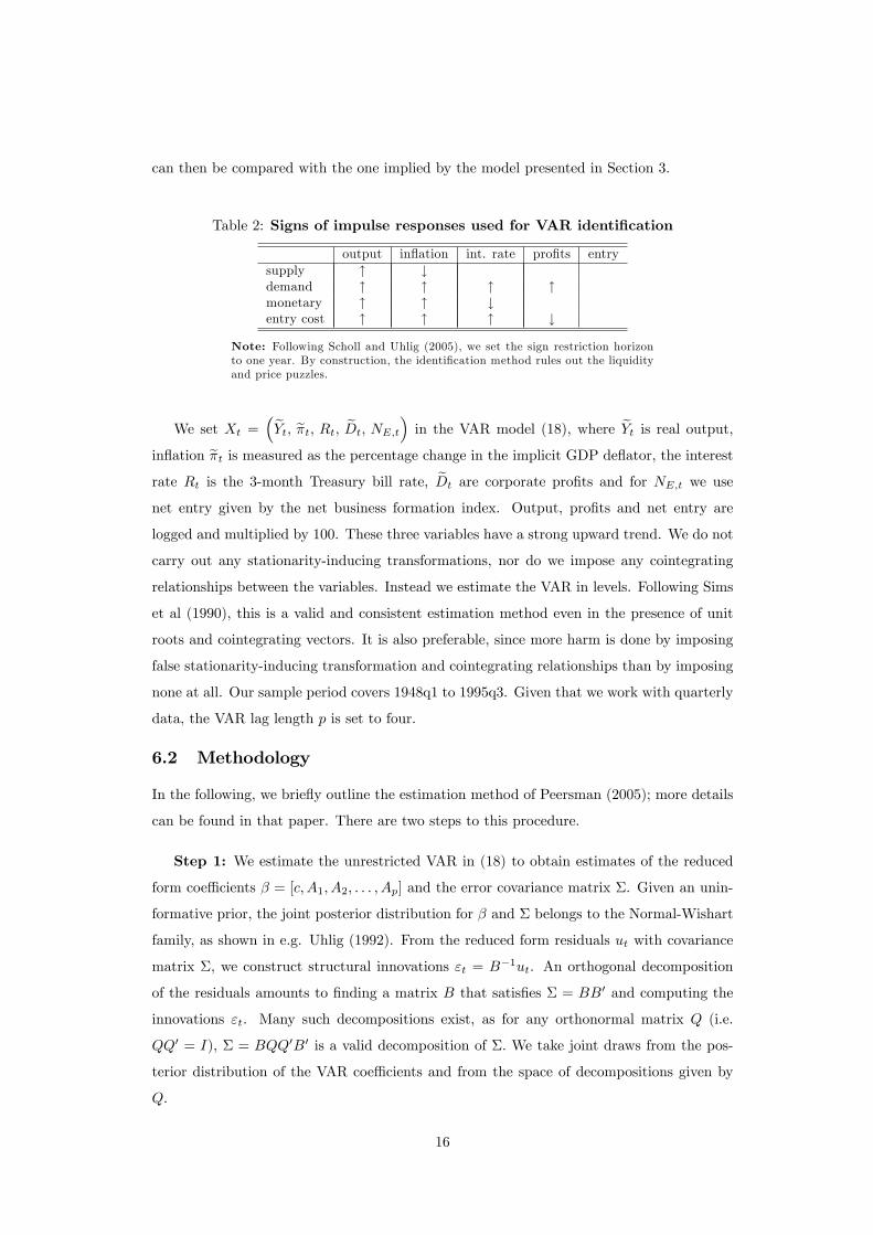
Further evidence on �rm dynamics in the macroeconomy come from vector autoregres-

sions. Bergin and Corsetti (2005) estimate a 5-variable VAR, using a recursive method to

identify monetary policy shocks. When �rm entry is measured as an index of net business

formation, they �nd that entry responds positively to expansionary monetary policy shocks.

We replicate their exercise; the results and details of the VAR ordering are given in the

appendix. As we see in Figure 3, the response of the entry-variable to monetary policy

shocks is signi�cant and exhibits a hump-shaped pro�le.

3 A macro model with �rm dynamics

In this section, we present a dynamic stochastic general equilibrium (DSGE) model of a

closed economy. In contrast to contributions such as Christiano et al (2005) and Smets

and Wouters (2003) who assume a variable capital stock and a �xed number of producers,

we abstract from variations in capital and instead endogenise the number of �rms. This

requires two assumptions: �rstly, love of variety in consumption and secondly, a sunk entry

cost and free entry in production.

4

3.1 Household preferences and intratemporal consumption choice

The economy is populated by a continuum of in�nitely-lived households, indexed by h 2

(0; 1). Each household maximises expected lifetime utility

Et

1Xs=0

�s"bt+sUt+s (h)

where � is the subjective discount factor and "bt+s is a consumption preference shock, which

is assumed to follow an AR(1) process. Period t utility is a positive function of consumption,

Ct (h), and a negative function of labour e¤ort, Lt (h),

Ut (h) =1

1� Ct (h)1� � �t

1 + 'Lt (h)

1+'

where is the inverse of the intertemporal elasticity of substitution, ' is the inverse of the

elasticity of labour supply with respect to the real wage and �t is a labour supply shock

following an AR(1) process. The consumption utility enjoyed by household h is de�ned over

a �xed set of di¤erentiated varieties, indexed by !

Ct (h) = At

�Z!2

ct (!; h)��1� d!

� ���1

(1)

where

At � N�� 1

��1t

� is the elasticity of substitution between goods, Nt is the number of varieties consumed

and � > 0 is the degree of love of variety (LOV).2 We do not consider the case where

� < 0, which implies that consumers dislike variety. If � = 0, agents are indi¤erent between

consuming more or fewer varieties. Note that At > 1 if the love of variety is higher than

the Dixit-Stiglitz (1977) benchmark, i.e. if � > 1��1 . Only a subset of goods t � is

available at time t. The consumption-based price index is the minimum cost of one unit of

the consumption bundle Ct (h). With the speci�cation of utility in (1), the associated price

index is

Pt =1

At

�Z!2t

pt (!)1��

d!

� 11��

(2)

where pt (!) is the price of variety !. The intratemporal optimisation problem for the

representative agent h is to choose ct (!; h) to maximise Ct (h), given total expenditureR!2t pt (!) ct (!; h) d!. Household demand for each individual good is

ct (!; h) = A��1t

�pt (!)

Pt

���Ct (h) (3)

2This de�nition of the consumption bundle disentangles the elasticity of substitution, which capturesthe degree of competition, from the taste for variety, which is a preference parameter. More details on thisdistinction can be found in Dixit and Stiglitz (1975) or Benassy (1996).

5

3.2 Government

For simplicity, we suppose that the government has the same consumption preferences as

the household, with elasticity of substitution � and love of variety �.

Gt = At

�Z!2

gt (!)��1� d!

� ���1

This implies that the price of one unit of Gt is given by (2) and that government demand

for variety ! is analogous to private demand

gt (!) = A��1t

�pt (!)

Pt

���Gt (4)

The government budget constraint is Gt = Tt, where government spending Gt is exogenous

and follows an AR(1) process (in logs). Tt denotes net lump sum taxes.

3.3 Firms

Each �rm uses the whole range of labour types to produce a single variety !, given the

following production technology

yt (!) = ZC;tlC;t (!) (5)

Manufacturing productivity, ZC;t, measures the e¢ ciency of one labour unit in producing

consumption goods. ZC;t is exogenous and follows an AR(1) process (in logs). The labour

input is de�ned as a bundle over all labour types

lC;t (!) ��Z 1

0

lC;t (h; !)��1� dh

� ���1

where lC;t (h; !) is the �rm�s demand for labour type h in the production of variety ! and

� is the elasticity of substitution between labour types. The economy-wide wage index is

the minimum cost of one unit of the labour bundle lC;t, which turns out to be symmetric

across �rms

Wt =

�Z 1

0

Wt (h)1��

dh

� 11��

where Wt (h) is the wage received by worker h. Pro�t-maximising �rms set prices pt (!) as

a constant markup over marginal cost. A �rm�s relative price, de�ned as �t (!) � pt (!) =Pt,

is therefore

�t (!) =�

� � 1wtZC;t

(6)

where wt �Wt=Pt is the real wage. Operating pro�ts (not taking into account entry costs)

are given by

dt (!) =1

��t (!) yt (!) (7)

6

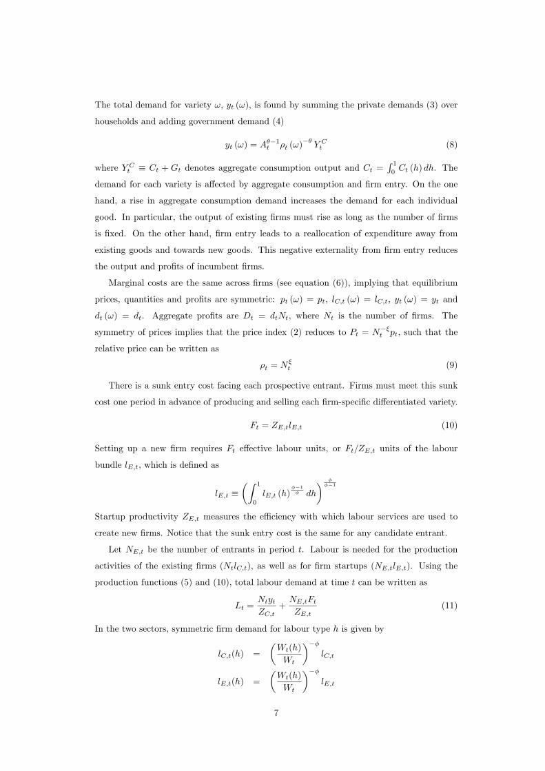
The total demand for variety !, yt (!), is found by summing the private demands (3) over

households and adding government demand (4)

yt (!) = A��1t �t (!)

��Y Ct (8)

where Y Ct � Ct + Gt denotes aggregate consumption output and Ct =R 10Ct (h) dh. The

demand for each variety is a¤ected by aggregate consumption and �rm entry. On the one

hand, a rise in aggregate consumption demand increases the demand for each individual

good. In particular, the output of existing �rms must rise as long as the number of �rms

is �xed. On the other hand, �rm entry leads to a reallocation of expenditure away from

existing goods and towards new goods. This negative externality from �rm entry reduces

the output and pro�ts of incumbent �rms.

Marginal costs are the same across �rms (see equation (6)), implying that equilibrium

prices, quantities and pro�ts are symmetric: pt (!) = pt, lC;t (!) = lC;t, yt (!) = yt and

dt (!) = dt. Aggregate pro�ts are Dt = dtNt, where Nt is the number of �rms. The

symmetry of prices implies that the price index (2) reduces to Pt = N��t pt, such that the

relative price can be written as

�t = N�t (9)

There is a sunk entry cost facing each prospective entrant. Firms must meet this sunk

cost one period in advance of producing and selling each �rm-speci�c di¤erentiated variety.

Ft = ZE;tlE;t (10)

Setting up a new �rm requires Ft e¤ective labour units, or Ft=ZE;t units of the labour

bundle lE;t, which is de�ned as

lE;t ��Z 1

0

lE;t (h)��1� dh

� ���1

Startup productivity ZE;t measures the e¢ ciency with which labour services are used to

create new �rms. Notice that the sunk entry cost is the same for any candidate entrant.

Let NE;t be the number of entrants in period t. Labour is needed for the production

activities of the existing �rms (NtlC;t), as well as for �rm startups (NE;tlE;t). Using the

production functions (5) and (10), total labour demand at time t can be written as

Lt =NtytZC;t

+NE;tFtZE;t

(11)

In the two sectors, symmetric �rm demand for labour type h is given by

lC;t(h) =

�Wt(h)

Wt

���lC;t

lE;t(h) =

�Wt(h)

Wt

���lE;t

7

Total demand for labour type h is therefore

Lt(h) = NtlC;t (h) +NE;tlE;t (h)

=

�Wt(h)

Wt

���Lt

3.4 Household budget constraint and intertemporal decisions

The household�s period budget constraint is

Bt (h)

Pt+wtNE;t (h)

ZE;t+ Ct (h) + Tt (h) = Rt

Bt�1 (h)

Pt+ dtNt (h) + wt (h)Lt (h) (12)

On the income side, we have gross interest income on bond holdings Bt (h), pro�t income,

and wage income. On the expenditure side, we have purchases of bonds, investment in new

�rms, consumption, and lump-sum taxes. Rt � 1 + it denotes the gross interest rate on

holdings of nominal bonds between t� 1 and t.

Maximising utility with respect to consumption Ct (h), subject to the budget constraint,

gives the following �rst order condition

�t = "btC

� t

where �t is the Lagrange multiplier on the budget constraint (12). We have dropped the

index h from this expression as we assume that there are state-contingent securities markets

that allow for complete consumption risk sharing across households, such that �t (h) = �t

for all h.

The household further chooses Bt (h) to maximise utility subject to the budget con-

straint, which yields the familiar Euler equation for bond holdings

�t = �RtEt

�PtPt+1

�t+1

�(13)

Firm entry displays some inertia in response to monetary policy shocks (see Bergin and

Corsetti (2005)). To account for this feature, we introduce a formulation of adjustment

costs commonly used in models with physical capital.3 Here, these adjustment costs apply

to �rm creation rather than to investment. Without adjustment costs in setting up �rms,

the response of NE;t to monetary policy shocks is very large on impact, implying a coun-

terfactually large conditional volatility of �rm entry. The number of �rms in period t+1 is

given by

Nt+1 = (1� �)Nt + F (NE;t; NE;t�1) (14)

where �rm entry is determined by the function F (�) de�ned as

F (NE;t; NE;t�1) ��1� S

�NE;tNE;t�1

��NE;t

3See appendix to Christiano, Eichenbaum and Evans (2005).

8

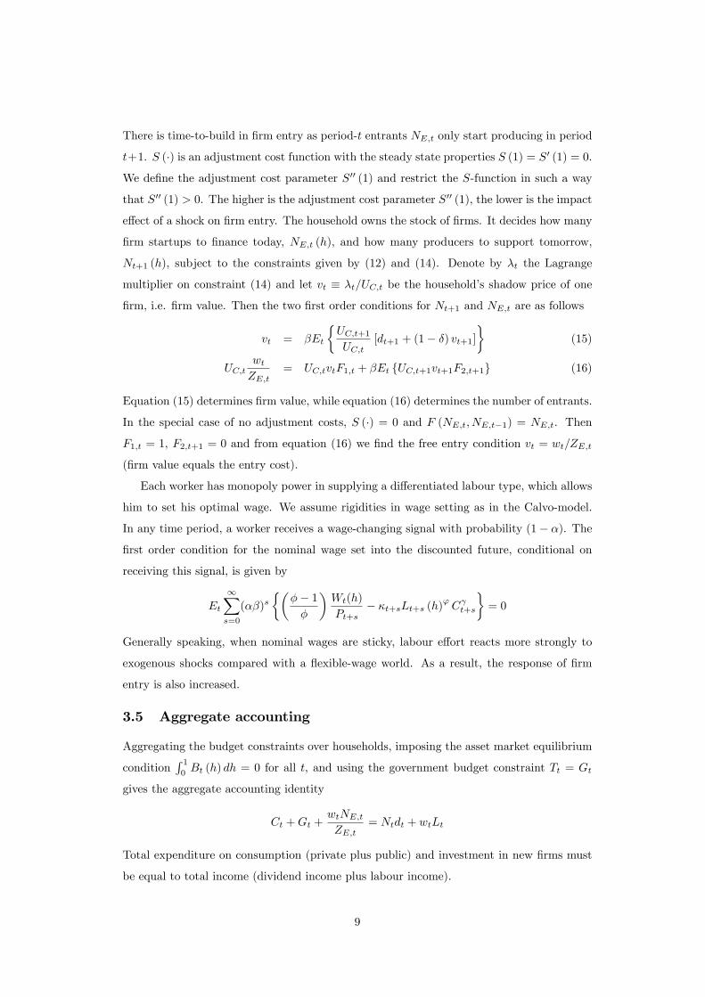
There is time-to-build in �rm entry as period-t entrants NE;t only start producing in period

t+1. S (�) is an adjustment cost function with the steady state properties S (1) = S0 (1) = 0.

We de�ne the adjustment cost parameter S00 (1) and restrict the S-function in such a way

that S00 (1) > 0. The higher is the adjustment cost parameter S00 (1), the lower is the impact

e¤ect of a shock on �rm entry. The household owns the stock of �rms. It decides how many

�rm startups to �nance today, NE;t (h), and how many producers to support tomorrow,

Nt+1 (h), subject to the constraints given by (12) and (14). Denote by �t the Lagrange

multiplier on constraint (14) and let vt � �t=UC;t be the household�s shadow price of one

�rm, i.e. �rm value. Then the two �rst order conditions for Nt+1 and NE;t are as follows

vt = �Et

�UC;t+1UC;t

[dt+1 + (1� �) vt+1]�

(15)

UC;twtZE;t

= UC;tvtF1;t + �Et fUC;t+1vt+1F2;t+1g (16)

Equation (15) determines �rm value, while equation (16) determines the number of entrants.

In the special case of no adjustment costs, S (�) = 0 and F (NE;t; NE;t�1) = NE;t. Then

F1;t = 1, F2;t+1 = 0 and from equation (16) we �nd the free entry condition vt = wt=ZE;t

(�rm value equals the entry cost).

Each worker has monopoly power in supplying a di¤erentiated labour type, which allows

him to set his optimal wage. We assume rigidities in wage setting as in the Calvo-model.

In any time period, a worker receives a wage-changing signal with probability (1� �). The

�rst order condition for the nominal wage set into the discounted future, conditional on

receiving this signal, is given by

Et

1Xs=0

(��)s��

�� 1�

�Wt(h)

Pt+s� �t+sLt+s (h)' C t+s

�= 0

Generally speaking, when nominal wages are sticky, labour e¤ort reacts more strongly to

exogenous shocks compared with a �exible-wage world. As a result, the response of �rm

entry is also increased.

3.5 Aggregate accounting

Aggregating the budget constraints over households, imposing the asset market equilibrium

conditionR 10Bt (h) dh = 0 for all t, and using the government budget constraint Tt = Gt

gives the aggregate accounting identity

Ct +Gt +wtNE;tZE;t

= Ntdt + wtLt

Total expenditure on consumption (private plus public) and investment in new �rms must

be equal to total income (dividend income plus labour income).

9

3.6 Monetary policy

To close the model, we assume the following linearised interest rate rule, with hats denoting

percentage deviations from steady state.

bRt = (1� �) h�0e�t +�1 �bYt � bY ft �i+ � bRt�1 + �Rtwhere �Rt is a white noise monetary policy shock and the parameter � determines the

degree of interest rate smoothing. The interest rate adjusts partially to CPI in�ation e�t �ln (pt=pt�1) and to the output gap (bYt � bY ft ). bY ft is de�ned as the level of output under

the assumption of perfectly �exible wages, i.e. � = 0. We suppose here that the central

bank does not observe the welfare-based price index Pt, but instead measures in�ation as

the change in average prices pt.4 See discussion in Section 5. CPI in�ation can be written

as e�t = �t + �( bNt � bNt�1) (17)

where welfare-based in�ation is given by the identity �t � !t�� bwt and !t denotes nominalwage in�ation, ie. !t � ln (Wt=Wt�1). Notice that the measure of the output gap is the

same whether Pt or pt is used as the de�ator.

4 Steady state

In the steady state, all endogenous variables are constant. Price and wage in�ation are equal

to zero, �t = !t = 0. Furthermore, all exogenous variables are also constant, ZC;t = ZC ,

Gt = G, �t = �, "bt = "b, ZE;t = ZE and �Rt = 0.

Given that F (NE ; NE) = NE , the law of motion for �rms (14) in steady state becomes

N = NE=�. The interest rate is obtained from the bond Euler equation (13), ��1 =

R = 1 + i. The ratio of pro�ts to �rm value is given by d=v = r + � through the �rm

value equation (15), where r is the (net) real interest rate. The share of pro�t income in

consumption output is found by combining equations (7) and (8)

dN

Y C=1

�

Using this result together with the expressions N = NE=� and d=v = r+�, we get the share

of investment in consumption output

vNEY C

=1

�

�

r + �

Noting that Y = Y C + vNE , the shares of investment and pro�t income in GDP are

4The results are qualitatively unchanged if we assume that the central bank observes Pt.

10

respectively

vNEY

=�

� + � (r + �)

dN

Y=

r + �

� + � (r + �)

The share of labour income in total income is

wL

Y= 1� r + �

� + � (r + �)

Denote by � the steady state share of government consumption in total consumption output,

i.e. � � G=Y C . The shares of government and private consumption in GDP are respectively

G

Y=

� (r + �)

� + � (r + �)�

C

Y=

(1� �) � (r + �)� + � (r + �)

Writing the labour demand equation (11) in steady state and substituting the steady state

versions of the entry equation (16), the law of motion for �rms (14), �rm value (15), pro�ts

(7), and �rm pricing (6), we �nd the labour shares in the two sectors

LCL

= 1� �

(r + �) � � rLEL

=�

(r + �) � � r

Note that all these ratios are independent of the steady state productivity levels ZC and

ZE . The model dynamics are thus una¤ected by steady state productivity.

5 Model dynamics

To compare the model with data, we need to strip out the e¤ect of varieties on the price

index. At present, CPI data does not account (adequately) for changes in consumption

utility arising from more or fewer available varieties. For any variable Xt in units of con-

sumption, the data-consistent counterpart is obtained as eXt � PtXt=pt = Xt=�t = XtN��t .

The e¤ect on the relative price �t is removed, because �t is always equal to 1 when changes

in the number of varieties are disregarded. Since �t is predetermined with respect to all

shocks, the impact e¤ect on the data-consistent variables does not di¤er from that on the

welfare-based variables. In general, the transition dynamics of the data-consistent variables

are qualitatively similar to the dynamics of the welfare-based variables. However, as can be

deduced from Table 4, there is no e¤ect of entry cost shocks, government spending shocks,

consumption preference shocks or monetary policy shocks on the data-consistent real wage,ewt. Also, a government spending shock has no e¤ect on the empirical measure of �rm value

11

evt. In the dynamic analysis below, we therefore focus on the following observable variablesthat react to all six shocks: eCt, Lt, eyt, eDt, NE;t, eYt, Rt, e�t. We describe the short runimpulse responses of those variables, assessing the e¤ects of transitory shocks to ZC;t, �t,

Gt, "bt , �Rt and ZE;t.

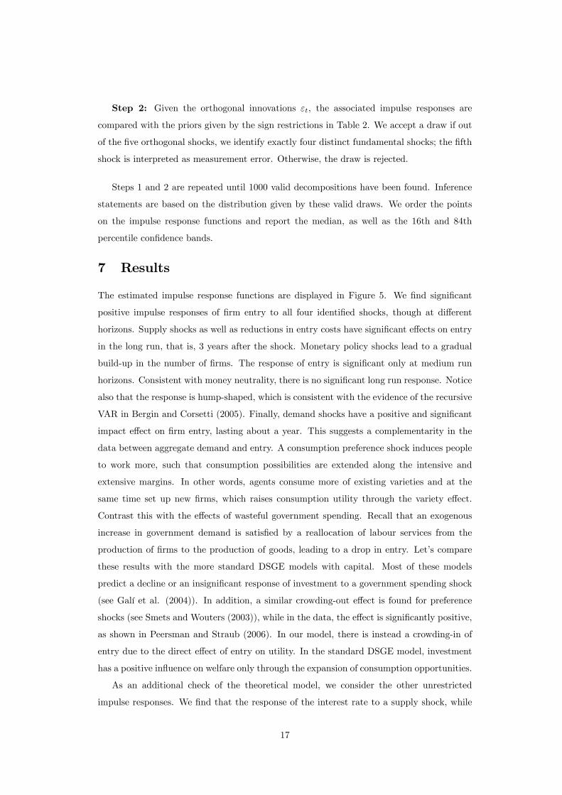
Figure 4 displays the impulse responses implied by the model for the variables eYt, e�t,Rt, eDt, NE;t which are the ones used in the empirical analysis in Section 6. The choice ofvariables will become clear later on. We perform a Monte Carlo simulation exercise as in

Peersman and Straub (2006). For each parameter, we choose a uniform distribution over

a range of values re�ecting previous estimates found in the literature. For details on the

parameter ranges, see Table 6. We take joint draws for all parameters and compute the

associated impulse responses. We report the median impulse response and the 16th and

84th percentile error bands based on 10,000 replications. Table 1 below summarises the

signs of the theoretical impulse responses, where the shocks have been given more general

names.

Table 1: Signs of impulse responses predicted by DSGE model

output in�ation int. rate pro�ts entrysupply " # # " "demand " " " " # or "monetary " " # " "entry cost " " " # "

Note that the e¤ect of a demand shock on �rm entry is ambiguous in the model.In response to a government spending shock, entry decreases, while followinga consumption preference shock, entry increases.

5.1 Supply shocks

Manufacturing productivity shock

A rise in manufacturing productivity (ZC;t) has a direct impact on the �rm�s pricing decision.

Each �rm will lower its price in proportion to the fall in marginal costs. As the number

of producers (and through equation (9) also the relative price �t) is predetermined, this

results in an equiproportionate drop in the aggregate price level. The welfare-based real

wage rises as the price level falls, which represents a spillover from the production sector to

the investment sector. On the one hand, the increase in the real wage implies a rise in entry

costs, which has a negative e¤ect on entry. On the other hand, the demand for each existing

variety increases due to a rise in aggregate consumption demand. This has a positive e¤ect

on pro�ts, which encourages entry. For a plausible set of parameter values, this second e¤ect

dominates and �rm entry is positive on impact. Output rises and in�ation falls in response

12

to a manufacturing productivity shock. The decrease in in�ation dominates the increase in

the output gap in our interest rate rule, resulting in a monetary policy expansion.

Labour supply shock

In boosting the economy�s productive capacity, a positive labour supply shock has similar

e¤ects as a productivity shock. Additional labour e¤ort allows for an increase in both con-

sumption and �rm entry, leading to an overall output expansion. Production initially rises

along the intensive margin (existing �rms produce more), and later on along the extensive

margin (new �rms enter). Firm output and pro�ts rise on impact. There is a drop in prices,

which brings about a loosening of the monetary policy stance.

5.2 Demand shocks

Government spending shock

On impact, a government spending shock (Gt) crowds out private consumption. This crowd-

ing out is only partial, such that output rises. The resulting positive output gap and in�ation

induce the monetary authority to raise the interest rate. Since the number of producers is

�xed initially, the rise in aggregate demand pushes up �rm output and pro�ts. As pro-

ductivity is unchanged, the increased production by existing �rms is achieved through a

rise in labour e¤ort. Assuming realistic values for the labour supply elasticity, the extra

demand from government spending has to be met by reallocating labour away from the

entrepreneurial sector to the production sector. As a consequence, �rm entry falls.

Consumption preference shock

Suppose that an exogenous shock to private consumption demand hits the economy. This rise

in demand can be satis�ed in two di¤erent ways. Agents can raise their current consumption

of existing varieties, which requires an increase in the labour input of producing �rms. An

alternative way to raise consumption utility is through the introduction of new varieties (at

least if the shock is persistent). Here, additional labour is needed for �rm startups. Both

consumption and �rm entry are positively a¤ected by the preference shock, giving rise to

a positive output gap and in�ation. The central bank responds by increasing the interest

rate. Initially, incumbents bene�t from higher pro�ts, because the stock of �rms is slow to

adjust. Gradually, however, these excess pro�ts are eroded as new entrants claim market

share.

5.3 Monetary policy shocks

An expansionary monetary policy shock is modelled as a drop in the interest rate. This

creates a boost to consumption and �rm entry. Given that �exible-wage output has not

13

changed, the output gap becomes positive. With constant productivity, an increase in

production requires an increase in labour e¤ort. As all �rms raise prices, in�ation becomes

positive. In the shock period, the increased consumption demand induces �rms to raise

their output, which they sell at the predetermined relative price �t. Thus, pro�ts increase

on impact.

5.4 Entry cost shocks

A positive shock to startup productivity (ZE;t) lowers entry costs. Similar to an investment-

speci�c productivity shock, it does not a¤ect the productivity of existing �rms, but makes

investment into new ones more attractive. Consumption falls initially in order to �nance the

entry of new �rms. Labour e¤ort rises to accommodate the increased demand of entrants.

As aggregate consumption demand falls, each incumbent sees his �rm-speci�c demand curve

shift inwards, such that �rm output drops. Since relative prices (�t), are unchanged initially,

lower �rm output also implies lower (real) pro�ts. A shock to ZE;t leads to a positive output

gap (driven by an expansion in �rm startups) and in�ation, which induces a monetary

tightening by the central bank.

6 A vector autoregression with sign restrictions5

Our aim is to study the dynamic e¤ects of exogenous shocks on �rm entry and compare

them with the model predictions of Section 5. For this purpose, we estimate a vector

autoregression (VAR) with subset of the variables of our model

Xt = c+

pXj=1

AjXt�j +B"t (18)

where c is a vector of constants and linear trends, Xt is an n � 1 vector of variables, Ajare coe¢ cient matrices and "t are normally distributed, mutually and serially uncorrelated

innovations with unit variance, i.e. "t � N (0; I). More speci�cally, "t =�"St ; "

Dt ; "

Mt ; "

Et

�,

where "St is a supply shock, "Dt is a demand shock, "

Mt is a monetary policy shock and "Et is

an entry cost shock. Since we have little empirical evidence on how �rm entry responds to

aggregate shocks, we do not want to be too speci�c about the precise nature of the underlying

shocks. Instead, we identify classes of shocks. Supply shocks encompass productivity shocks

and labour supply shocks. Government spending shocks and preference shocks are classi�ed

as demand shocks. Note that entry cost shocks look similar to demand shocks as they

raise output, in�ation and interest rates. However, we want to identify entry cost shocks

separately for two reasons. Firstly, these shocks are speci�c to models with �rm endogeneity,

5Examples of VARs with sign restrictions can be found in Faust (1998), Uhlig (2005), Canova and DeNicoló (2002).

14

which is the focus of the paper. Secondly, in standard models with a variable capital stock

and a �xed number of �rms, investment-speci�c technology shocks are an important source

of output �uctuations (see Fisher (2002)).

6.1 Choice of variables and identi�cation

The variables chosen from the theory in Section 3 must satisfy two conditions. Firstly, they

must be empirically observable, i.e. the variables that are expressed in real terms must be

de�ated by the CPI equivalent in the model, which is pt (rather than the welfare-based price

index Pt). Secondly, their short run responses to the exogenous shocks must be su¢ ciently

di¤erent from each other as to allow for the identi�cation of each shock. In choosing a

subset of variables for our VAR, we are further guided by Peersman and Straub (2006).

They summarise the controversies that currently exist in the literature on standard DSGE

models with capital. These are, �rstly, the e¤ect of government spending on investment

and consumption; secondly, the e¤ect of technology shocks on labour e¤ort; and thirdly, the

e¤ect of demand side shocks on the real wage. Of these controversial responses, we consider

only that of investment (which in our model corresponds to �rm entry) to government

spending shocks. We do not use data on consumption, labour or wages in our empirical

analysis.

Given these considerations, we select four empirically observable variables that provide

su¢ cient information to identify all four types of shocks. These are real GDP, in�ation,

the interest rate and aggregate pro�ts (in real terms). A description of the data is given

in the appendix. Our identi�cation scheme is presented in Table 2 below. We adopt the

convention that a positive shock is one that increases output temporarily. We look at the

impulse responses of the other three variables in relation to the output response. Firstly,

we identify a supply shock by its negative e¤ect on in�ation. Secondly, of those shocks that

lead to positive in�ation, we single out monetary shocks as those that reduce the nominal

interest rate. The restrictions used to identify these two shocks are robust across a range

of models and as such widely accepted, as noted by Peersman and Straub (2006). Finally,

of those shocks that raise in�ation and the interest rate, we distinguish entry cost shocks

from (other) demand shocks by looking at their e¤ect on aggregate pro�ts. An entry cost

shock reduces pro�ts, while a demand shock raises pro�ts. Notice that these restrictions

are su¢ cient to fully identify the shocks. In addition to these four variables, we include a

measure of �rm entry in the VAR. The responses of �rm entry to the various shocks are

intentionally left unrestricted and are therefore fully determined by the data. In addition,

the response of the nominal interest rate and pro�ts to a manufacturing productivity shock

and the response of pro�ts to a monetary shock are left unrestricted. The estimated response

15

can then be compared with the one implied by the model presented in Section 3.

Table 2: Signs of impulse responses used for VAR identi�cation

output in�ation int. rate pro�ts entrysupply " #demand " " " "monetary " " #entry cost " " " #

Note: Following Scholl and Uhlig (2005), we set the sign restriction horizonto one year. By construction, the identi�cation method rules out the liquidityand price puzzles.

We set Xt =�eYt, e�t, Rt, eDt, NE;t� in the VAR model (18), where eYt is real output,

in�ation e�t is measured as the percentage change in the implicit GDP de�ator, the interestrate Rt is the 3-month Treasury bill rate, eDt are corporate pro�ts and for NE;t we usenet entry given by the net business formation index. Output, pro�ts and net entry are

logged and multiplied by 100. These three variables have a strong upward trend. We do not

carry out any stationarity-inducing transformations, nor do we impose any cointegrating

relationships between the variables. Instead we estimate the VAR in levels. Following Sims

et al (1990), this is a valid and consistent estimation method even in the presence of unit

roots and cointegrating vectors. It is also preferable, since more harm is done by imposing

false stationarity-inducing transformation and cointegrating relationships than by imposing

none at all. Our sample period covers 1948q1 to 1995q3. Given that we work with quarterly

data, the VAR lag length p is set to four.

6.2 Methodology

In the following, we brie�y outline the estimation method of Peersman (2005); more details

can be found in that paper. There are two steps to this procedure.

Step 1: We estimate the unrestricted VAR in (18) to obtain estimates of the reduced

form coe¢ cients � = [c; A1; A2; : : : ; Ap] and the error covariance matrix �. Given an unin-

formative prior, the joint posterior distribution for � and � belongs to the Normal-Wishart

family, as shown in e.g. Uhlig (1992). From the reduced form residuals ut with covariance

matrix �, we construct structural innovations "t = B�1ut. An orthogonal decomposition

of the residuals amounts to �nding a matrix B that satis�es � = BB0 and computing the

innovations "t. Many such decompositions exist, as for any orthonormal matrix Q (i.e.

QQ0 = I), � = BQQ0B0 is a valid decomposition of �: We take joint draws from the pos-

terior distribution of the VAR coe¢ cients and from the space of decompositions given by

Q.

16

Step 2: Given the orthogonal innovations "t, the associated impulse responses are

compared with the priors given by the sign restrictions in Table 2. We accept a draw if out

of the �ve orthogonal shocks, we identify exactly four distinct fundamental shocks; the �fth

shock is interpreted as measurement error. Otherwise, the draw is rejected.

Steps 1 and 2 are repeated until 1000 valid decompositions have been found. Inference

statements are based on the distribution given by these valid draws. We order the points

on the impulse response functions and report the median, as well as the 16th and 84th

percentile con�dence bands.

7 Results

The estimated impulse response functions are displayed in Figure 5. We �nd signi�cant

positive impulse responses of �rm entry to all four identi�ed shocks, though at di¤erent

horizons. Supply shocks as well as reductions in entry costs have signi�cant e¤ects on entry

in the long run, that is, 3 years after the shock. Monetary policy shocks lead to a gradual

build-up in the number of �rms. The response of entry is signi�cant only at medium run

horizons. Consistent with money neutrality, there is no signi�cant long run response. Notice

also that the response is hump-shaped, which is consistent with the evidence of the recursive

VAR in Bergin and Corsetti (2005). Finally, demand shocks have a positive and signi�cant

impact e¤ect on �rm entry, lasting about a year. This suggests a complementarity in the

data between aggregate demand and entry. A consumption preference shock induces people

to work more, such that consumption possibilities are extended along the intensive and

extensive margins. In other words, agents consume more of existing varieties and at the

same time set up new �rms, which raises consumption utility through the variety e¤ect.

Contrast this with the e¤ects of wasteful government spending. Recall that an exogenous

increase in government demand is satis�ed by a reallocation of labour services from the

production of �rms to the production of goods, leading to a drop in entry. Let�s compare

these results with the more standard DSGE models with capital. Most of these models

predict a decline or an insigni�cant response of investment to a government spending shock

(see Galí et al. (2004)). In addition, a similar crowding-out e¤ect is found for preference

shocks (see Smets and Wouters (2003)), while in the data, the e¤ect is signi�cantly positive,

as shown in Peersman and Straub (2006). In our model, there is instead a crowding-in of

entry due to the direct e¤ect of entry on utility. In the standard DSGE model, investment

has a positive in�uence on welfare only through the expansion of consumption opportunities.

As an additional check of the theoretical model, we consider the other unrestricted

impulse responses. We �nd that the response of the interest rate to a supply shock, while

17

negative in the model, is insigni�cant in the data. There are two o¤setting in�uences on

the interest rate in the monetary policy rule: on the one hand, a positive output gap calls

for a monetary tightening; on the other hand, a fall in prices calls for a monetary easing.

The model prediction of a net monetary easing is a consequence of perfect price �exibility.

The fall in in�ation dominates the rise in the output gap. With �exible prices, the weight

on in�ation stabilisation should be reduced compared with the sticky-price benchmark on

which the parameter ranges of Table 6 are based. Pro�ts react positively to supply shocks at

short horizons; the long run e¤ect is insigni�cant. Following a monetary policy expansion,

pro�ts increase in a hump-shaped fashion, �rst becoming signi�cantly positive, followed by

a signi�cantly negative response at longer horizons. This is consistent with our theoretical

model. At �rst, the rise in aggregate demand drives up the pro�ts of existing �rms. The

increase in pro�tability induces new �rm startups, but with some delay. Firm entry leads to

some expenditure switching from old to new goods, thereby reducing the pro�ts of incumbent

�rms.

Turning to the variance decompositions in Table 7, it is worth noting that shocks to entry

costs do not explain a large proportion of the �uctuations in �rm entry. Demand shocks play

a much bigger role. This is consistent with the observation that overall, entry is procyclical,

whereas entry cost shocks give rise to countercyclical movements in entry. It might also

re�ect the fact that entry costs depend to a large extent on institutional arrangements,

which are slow to change.

8 Conclusion

The aim of this paper is to improve our understanding of the driving forces of �rm entry and

exit over the business cycle. We have built a DSGE model with an endogenous number of

�rms, featuring the main classes of macroeconomic shocks. In addition to supply, demand

and monetary shocks, we allow for shocks to entry costs. Using a minimum set of robust sign

restrictions implied by our model, we identify a VAR. Firm entry is allowed to respond freely

to the four shocks. The responses are in line of what our theory predicts. One notable �nding

is that of a positive e¤ect of an increase in demand on entry, consistent with the impulse

response predicted by a consumption preference shock. This shows that aggregate demand

disturbances lead to important adjustments in consumption output along the extensive

margin. Moreover, �rm entry responds signi�cantly to all kinds of macroeconomic shocks.

This �nding has far-reaching implications. Firstly, if every �rm produces a di¤erentiated

good, �uctuations in the number of �rms proxy �uctuations in the composition of the

consumption basket. Such �uctuations entail welfare e¤ects and raise doubts about the

18

measurement of a price index as the price of a static bundle of goods. Secondly, �rm entry

might in�uence the degree of competition. Although beyond the scope of the present paper,

endogenous markups that depend on the number of �rms are an interesting topic for future

research. Thirdly, how are stabilisation policies a¤ected by the insights that a) output

�uctuations have an intensive as well as an extensive margin, and b) that the (correctly

measured) price index re�ects average prices as well as the number of consumption varieties?

A �rst attempt to answer this question is given in Bergin and Corsetti (2005). This paper

provides evidence of the importance of their enquiry. Finally, another challenge is to extend

the analysis to an open economy. A fast-growing country can channel its productivity

into the increased production of existing goods, or it can expand the gamma of varieties

it produces. Whether export growth is along the extensive margin (more varieties) or the

intensive margin (greater volumes) has very di¤erent implications for the terms of trade and

for international spillovers.

References

[1] Benassy, J-P. (1996), Taste for variety and optimum production patterns in monopo-

listic competition, Economics Letters 52, p. 41-47.

[2] Bergin, P. and G. Corsetti (2005), Towards a theory of �rm entry and stabilization

policy, NBER Working Paper number 11821.

[3] Bilbiie, F.O., F. Ghironi and M.J. Melitz (2005), Business cycles and �rm dynamics,

manuscript.

[4] Broda, C. and D. Weinstein (2004), Globalization and the gains from variety, Federal

Reserve Bank of New York Sta¤ Report no. 180.

[5] Campbell, J.R. (1997), Entry, exit, embodied technology, and business cycles, NBER

Working Paper No. 5955.

[6] Canova, F. and G. De Nicoló (2002), Monetary disturbances matter for business �uc-

tuations in the G-7, Journal of Monetary Economics, vol. 49, issue 6, pages 1131-1159.

[7] Chatterjee, S. and R.W. Cooper (1993), Entry and exit, product variety and the busi-

ness cycle, NBER Working Paper No. 4562.

[8] Christiano, L.J., M. Eichenbaum and C.L. Evans (2005), Nominal rigidities and the

dynamic e¤ects of a shock to monetary policy, Journal of Political Economy, vol. 113,

no.1.

19

[9] Christiano, L.J., M. Eichenbaum and C.L. Evans (1999), Monetary policy shocks: what

have we learned and to what end?, in J.B. Taylor and M. Woodford (ed.) Handbook of

Macroeconomics, chapter 2, pages 65-148.

[10] Corsetti, G., P. Martin and P. Pesenti (2005), Productivity spillovers, terms of trade

and the �home market e¤ect�, NBER Working Paper No. 11165.

[11] Dixit, A.K. and J.E. Stiglitz (1975), Monopolistic competition and optimum product

diversity, Warwick Economic Research Paper number 64.

[12] Dixit, A.K. and J.E. Stiglitz (1977), Monopolistic competition and optimum product

diversity, American Economic Review, volume 6, number 3.

[13] Fisher, J.D.M. (2002), Technology shocks matter, Federal Reserve Bank of Chicago

Working Paper Series WP-02-14.

[14] Galí, J., J.D. López-Salido and J. Vallés (2004), Understanding the e¤ects of govern-

ment spending on consumption, ECB Working Paper No. 339.

[15] Ghironi, F. and M.J. Melitz (2005), International trade and macroeconomic dynamics

with heterogeneous �rms, Quarterly Journal of Economics, vol. 120(3), pages 865-915.

[16] Hausman, J. (1999), Cellular telephone, new products, and the CPI, Journal of Business

and Economic Statistics, volume 17, number 2.

[17] Hausman, J. (2002), Sources of bias and solutions to bias in the CPI, NBER Working

Paper No. 9298.

[18] Jaimovich, N. (2004), Firm Dynamics, Markup Variations, and the Business Cycle,

manuscript.

[19] Krugman, P.R. (1979), Increasing returns, monopolistic competition and international

trade, Journal of International Economics (9), pages 469-479.

[20] Peersman, G. (2005), What caused the early millennium slowdown? Evidence based

on vector autoregressions, Journal of Applied Econometrics, vol 20, p 185-207.

[21] Peersman G. and R. Straub (2006), Putting the New Keynesian Model to a Test: An

SVAR Analysis with DSGE Priors, manuscript.

[22] Scholl, A. and H. Uhlig (2005), New Evidence on the Puzzles. Results from Agnostic

Identi�cation on Monetary Policy and Exchange Rates, manuscript.

20

[23] Sims, C.A. J.H. Stock and M.W. Watson (1990), Inference in linear time series models

with some unit roots, Econometrica, Vol. 58, No.1, pages 113-144

[24] Smets, F. and R. Wouters (2004), Shocks and Frictions in US Business Cycles: A

Bayesian DSGE Approach, manuscript.

[25] Smets, F. and R. Wouters (2003), An Estimated Dynamic Stochastic General Equi-

librium Model of the Euro Area, Journal of the European Economic Association, vol.

1(5), pages 1123-1175.

[26] Uhlig, H. (2005), What are the e¤ects of monetary policy shocks on output? Results

from an agnostic identi�cation procedure, Journal of Monetary Economics 52, p 381-

419.

[27] Uhlig, H. (1994), What Macroeconomists Should Know about Unit Roots: A Bayesian

Perspective, Econometric Theory, vol. 10, issue 3-4, pages 645-71.

21

Appendix

Data

Data series are taken from the St. Louis Fed Economic Database, except for the data on

�rm entry. Net business formation (NBF) and New business incorporations (NI) are from

the BEA�s Survey of Current Business. These series have been discontinued; data run from

January 1948 to September 1995 (for NBF) and to September 1996 (for NI). VAR with sign

restrictions: In�ation is measured as the percentage change in the implicit GDP de�ator.

The interest rate is the 3-month Treasury bill rate. Pro�ts are de�ated using the GDP

de�ator. The commodity price variable in the recursive VAR is the change in the index of

sensitive materials prices, which is obtained from the Christiano et al (1999) data set.

Table 3: Data

Variable Units, Freq, Seas. adj. Series IDReal Gross Domestic Product, 1 Decimal Bil. Chn. 2000 $, Q, SAAR GDPC1CPI For All Urban Consumers: All Items Index 1982-84=100, M, SA CPIAUCSLCorporate Pro�ts with IVA and CCAdj Bil. $, SAAR, Q CPROFIT3-Month Treasury Bill: Second. Mkt. Rate %, M TB3MSE¤ective Federal Funds Rate %, M FEDFUNDSGDP: Implicit Price De�ator Index 2000=100, Q, SA GDPDEFNet business formation Index 1967=100, M -New business incorporations Thousands, M -Industrial Production Index Index 2002=100, M, SA INDPRONon-Borrowed Reserves of Depository Inst. Bil. $, M, SA BOGNONBRAggr. Reserves of Dep. Inst. & Monet. Base Bil. $, M, SA TRARRChange in sensitive materials prices CHGSMPS

Variable CHGSMPS from data appendix to Christiano, Eichenbaum and Evans (1999). IVA = InventoryValuation Adjustment, CCAdj = Capital Consumption Adjustment.

22

Linearised DSGE model

The model has sixteen endogenous variables: bAt, b�t, bdt, byt, bY Ct , bwt, bLt, bCt, bNt, bvt, bNE;t,!t, bYt, bRt, �t, e�t. We have seventeen equations; invoking Walras�law we can drop one ofthe market clearing conditions. Potential output Y ft is de�ned as the level of output under

perfectly �exible wages. In practice, the model is extended by a �exible wage block where

� = 0.

Table 4: Summary of the linearised model equations

bAt = �� � 1��1

� bNt auxiliary variableb�t = bwt � bZC;t price settingbdt = b�t + byt pro�tsbyt = (� � 1) bAt � �b�t + bY Ct �rm outputbY C

t = (1� �)� bCt + bGt� consumption outputb�t = � bNt relative pricebLt = LC

L

� bNt + byt � bZC;t�+ LEL

� bNE;t � bZE;t� labour demand

"bt � bCt = bRt � Et n�t+1 � "bt+1 + bCt+1o bondsbNt = (1� �) bNt�1 + � bNE;t�1 �rm law of motionbvt = Et n � bCt � bCt+1�+ 1��1+r

bvt+1 + r+�1+r

bdt+1o �rm valuebNE;t =1

1+�

� bNE;t�1 + �Etn bNE;t+1

o+ 1

S00(1)

hbvt � � bwt � bZE;t�i� free entry

!t =(1� ��) (1� �)� (1 + �')

�b�t + 'bLt + bCt � bwt�+ �Et!t+1 wage in�ationbYt = dNY

� bNt + bdt�+ wLY

� bwt � bLt� aggr. incomebYt = Y C

YbY Ct + vNE

Y

�bvt + bNE;t

�aggr. expenditurebRt = (1� �) h�0�t +�1 �bYt � bY f

t

�i+ � bRt�1 + �Rt monetary policy

�t = !t �� bwt welfare-based in�.e�t = �t + �( bNt � bNt�1) CPI in�ation

The model has six exogenous shocks: bZC;t, b�t, bGt, b"bt , bZE;t, �Rt . The �rst �ve are

AR(1) processes. Following Smets and Wouters (2004), the �t�s are assumed to be normally

distributed with mean zero and standard deviation 0.25.

Table 5: Summary of the exogenous shock processes

bZC;t = �zc bZC;t�1 + �zct manufacturing productivity shockb�t = ��b�t�1 + ��t labour supply shockbGt = �g bGt�1 + �gt government spending shockb"bt = �bb"bt�1 + �bt consumption preference shockbZE;t = �ze bZE;t�1 + �zet entry cost shock�Rt monetary policy shock

23

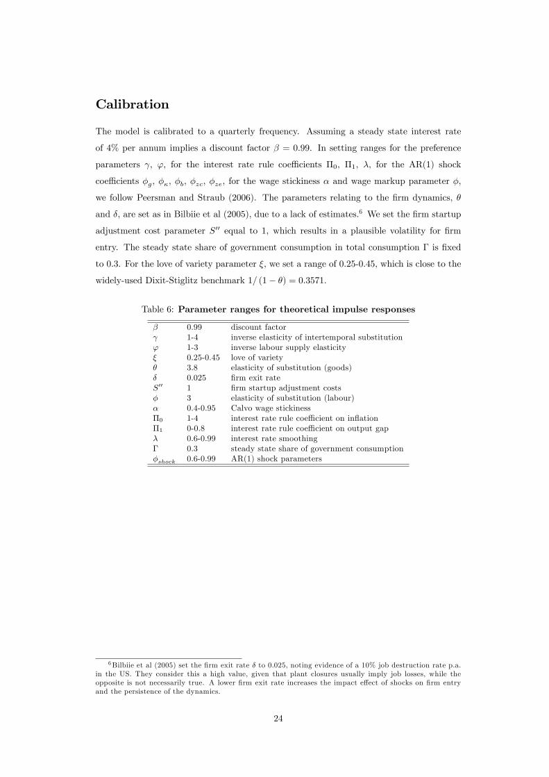
Calibration

The model is calibrated to a quarterly frequency. Assuming a steady state interest rate

of 4% per annum implies a discount factor � = 0:99. In setting ranges for the preference

parameters , ', for the interest rate rule coe¢ cients �0, �1, �, for the AR(1) shock

coe¢ cients �g, ��, �b, �zc, �ze, for the wage stickiness � and wage markup parameter �,

we follow Peersman and Straub (2006). The parameters relating to the �rm dynamics, �

and �, are set as in Bilbiie et al (2005), due to a lack of estimates.6 We set the �rm startup

adjustment cost parameter S00 equal to 1, which results in a plausible volatility for �rm

entry. The steady state share of government consumption in total consumption � is �xed

to 0.3. For the love of variety parameter �, we set a range of 0.25-0.45, which is close to the

widely-used Dixit-Stiglitz benchmark 1= (1� �) = 0:3571.

Table 6: Parameter ranges for theoretical impulse responses

� 0.99 discount factor 1-4 inverse elasticity of intertemporal substitution' 1-3 inverse labour supply elasticity� 0.25-0.45 love of variety� 3.8 elasticity of substitution (goods)� 0.025 �rm exit rateS00 1 �rm startup adjustment costs� 3 elasticity of substitution (labour)� 0.4-0.95 Calvo wage stickiness�0 1-4 interest rate rule coe¢ cient on in�ation�1 0-0.8 interest rate rule coe¢ cient on output gap� 0.6-0.99 interest rate smoothing� 0.3 steady state share of government consumption�shock 0.6-0.99 AR(1) shock parameters

6Bilbiie et al (2005) set the �rm exit rate � to 0.025, noting evidence of a 10% job destruction rate p.a.in the US. They consider this a high value, given that plant closures usually imply job losses, while theopposite is not necessarily true. A lower �rm exit rate increases the impact e¤ect of shocks on �rm entryand the persistence of the dynamics.

24

Figure 1: Cyclical component of net business formation

­20

­15

­10

­5

0

5

10

15

20

1948

1950

1952

1954

1956

1958

1960

1962

1964

1966

1968

1970

1972

1974

1976

1978

1980

1982

1984

1986

1988

1990

1992

1994

NBF real GDP

Figure 2: Cyclical component of new incorporations

­20

­15

­10

­5

0

5

10

15

20

1948

1950

1952

1954

1956

1958

1960

1962

1964

1966

1968

1970

1972

1974

1976

1978

1980

1982

1984

1986

1988

1990

1992

1994

1996

NI real GDP

These graphs show the cyclical components of �rm entry and real GDP in the US over the sampleperiod 1948q1-1995q3. Entry is measured as net business formation (top panel) and new incor-porations (bottom panel). The two series have been HP-�ltered with a smoothing parameter of1600.

25

Figure 3: Response of net business formation to innovation in federal funds rate(top panel) and in the nonborrowed reserves ratio (bottom panel)

­.012

­.010

­.008

­.006

­.004

­.002

.000

.002

5 10 15 20 25 30 35 40 45

­.004

.000

.004

.008

.012

.016

5 10 15 20 25 30 35 40 45

These graphs replicate the recursive VAR exercise in Bergin and Corsetti (2005). The variables inorder are as follows: log industrial production, log CPI, commodity prices, ratio of non-borrowedreserves to total reserves or federal funds rate, log net business formation. Replacing net businessformation by new incorporations in the VAR results in an insigni�cant response of the entryvariable to monetary policy shocks (not shown). The identi�cation scheme supposes a non-zerocontemporaneous e¤ect of monetary policy on industrial production, the CPI and commodityprices, but not on entry. Data is monthly. The sample period is January 1959 to June 1995. Thegraphs should be interpreted as follows. A one-standard-deviation rise in the federal funds rateleads to a drop in the net business formation index of 7% after 10 months.

26

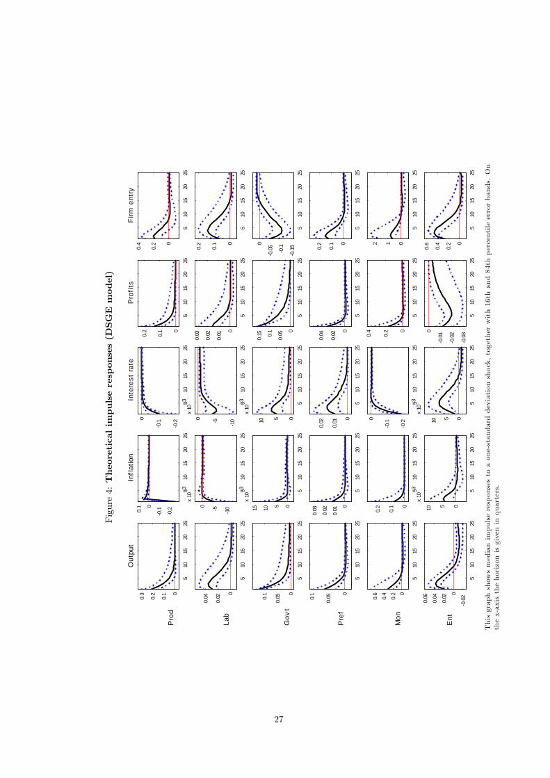
Figure4:Theoreticalimpulseresponses(DSGEmodel)

510

1520

25

0

0.1

0.2

0.3

Out

put

Pro

d

510

1520

25

­0.2

­0.1

0

0.1

Infl

atio

n

510

1520

25

­0.2

­0.1

0

Inte

rest

 rat

e

510

1520

25

0

0.1

0.2

Pro

fits

510

1520

25

0

0.2

0.4

Firm

 ent

ry

510

1520

25

0

0.02

0.04

Lab

510

1520

25

­10­50

x 10

­3

510

1520

25

­10­50

x 10

­3

510

1520

25

0

0.01

0.02

0.03

510

1520

25

0

0.1

0.2

510

1520

250

0.050.

1

Gov

t

510

1520

25

051015x 

10­3

510

1520

250510

x 10

­3

510

1520

25

0

0.050.

1

0.15

510

1520

25­0

.15

­0.1

­0.0

50

510

1520

25

0

0.050.

1

Pre

f

510

1520

25

0

0.01

0.02

0.03

510

1520

25

0

0.01

0.02

510

1520

25

0

0.02

0.04

510

1520

25

0

0.1

0.2

510

1520

25

00.

2

0.4

0.6

Mon

510

1520

25

0

0.1

0.2

510

1520

25

­0.2

­0.1

0

510

1520

25

0

0.2

0.4

510

1520

25

012

510

1520

25­0

.020

0.02

0.04

0.06

Ent

510

1520

25

0510

x 10

­3

510

1520

25

0510

x 10

­3

510

1520

25­0

.03

­0.0

2

­0.0

10

510

1520

25

0

0.2

0.4

0.6

Thisgraphshowsmedianimpulseresponsestoaone-standarddeviationshock,togetherwith16thand84thpercentileerrorbands.On

thex-axisthehorizonisgiveninquarters.

27

Figure5:Estimated

impulseresponses(VARmodel)

510

1520

25

0

0.2

0.4

0.6

Out

put

Sup

ply

510

1520

25­0

.4

­0.3

­0.2

­0.1

0

0.1

Infl

atio

n

510

1520

25­0

.3

­0.2

­0.1

0

0.1

0.2

Inte

rest

 rat

e

510

1520

25­10123

Pro

fits

510

1520

25

­0.5

0

0.5

Firm

 ent

ry

510

1520

25

0

0.2

0.4

0.6

0.81

Dem

and

510

1520

25

0

0.050.

1

0.150.

2

510

1520

25

0

0.2

0.4

0.6

510

1520

25

­2024

510

1520

25­0

.5

0

0.51

1.52

510

1520

25­0

.2

0

0.2

0.4

0.6

Mon

etar

y

510

1520

25

0

0.1

0.2

0.3

510

1520

25

­0.4

­0.2

0

0.2

510

1520

25

­1012

510

1520

25­0

.5

0

0.51

510

1520

25­0

.1

0

0.1

0.2

0.3

0.4

Ent

ry c

ost

510

1520

25­0

.050

0.050.

1

0.150.

2

510

1520

25

0

0.2

0.4

510

1520

25

­2­10

510

1520

25

­0.5

0

0.5

Thisgraphshowsmedianimpulseresponsestoaone-standarddeviationshock,togetherwith16thand84thpercentileerrorbands.On

thex-axisthehorizonisgiveninquarters.

28

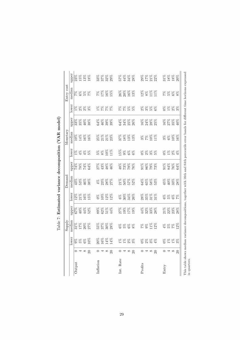
Table7:Estimated

variancedecom

position(VARmodel)

Supply

Demand

Monetary

Entrycost

lower

median

upper

lower

median

upper

lower

median

upper

lower

median

upper

Output

09%

31%

67%

12%

43%

74%

1%10%

33%

1%7%

23%

45%

17%

40%

21%

53%

78%

4%14%

35%

2%6%

15%

86%

20%

44%

16%

46%

74%

4%16%

40%

2%5%

13%

2010%

27%

52%

15%

38%

64%

5%16%

38%

3%7%

18%

In�ation

020%

55%

89%

0%4%

27%

5%25%

64%

1%7%

33%

416%

37%

62%

10%

23%

43%

8%21%

46%

7%17%

37%

814%

30%

51%

12%

28%

48%

10%

21%

39%

7%16%

32%

2014%

28%

44%

12%

27%

46%

11%

23%

39%

7%15%

29%

Int.Rate

01%

6%27%

6%21%

48%

15%

37%

64%

7%26%

57%

41%

5%19%

30%

50%

73%

9%18%

34%

7%20%

44%

82%

6%17%

34%

57%

79%

6%13%

25%

5%16%

34%

203%

8%19%

26%

52%

76%

6%13%

26%

5%13%

28%

Pro�ts

00%

7%44%

28%

64%

91%

0%3%

16%

2%12%

29%

42%

9%32%

35%

65%

86%

2%7%

24%

3%8%

17%

83%

11%

33%

31%

58%

79%

3%10%

28%

5%11%

21%

204%

12%

28%

31%

53%

73%

5%11%

25%

6%11%

22%

Entry

00%

4%21%

6%45%

91%

0%3%

16%

0%7%

31%

41%

5%22%

5%40%

84%

1%6%

27%

1%5%

18%

81%

7%23%

6%33%

76%

2%10%

35%

2%6%

18%

203%

12%

28%

7%28%

64%

4%16%

40%

3%8%

20%

Thistableshowsmedianvariancedecompositions,togetherwith16thand84thpercentileerrorbandsfordi¤erenttimehorizonsexpressed

inquarters.

29