Embed Size (px)
Citation preview

Dept of Real Estate and Construction Management Master of Science Thesis no. 501 Div of Building and Real Estate Economics
Macroeconomic Overview and the Correlations Between Selected Real Estate Markets
Stockholm – London – New York
Author: Supervisor: Johan Edenström Mats Wilhelmsson Olof Johnson
Stockholm 2010

2
Master of Science thesis
Title: Macroeconomic Overview and the Correlations
Between Selected Real Estate Markets
Stockholm – London – New York
Authors Johan Edenström and Olof Johnson
Department Department of Real Estate and Construction
Management
Division of Building and Real Estate Economics
Master Thesis number 501
Supervisor Mats Wilhelmsson
Keywords Real Estate, Correlation, Co-Movements, Time Lag
Abstract: Statements such as “there could be a time lag between real estate markets all over the globe” or that “there might be a correlation between different real estate markets” has been present for a long time. We are to investigate if there is some reality in these assumptions focusing on studying if there is a significant presence of correlations and co-movements between three selected real estate office markets. The following markets are undertaken in our study; Stockholm (Sweden), London (United Kingdom) and New York (United States) The first part of this thesis discusses the Fisher-Di Pasquale-Wheaton (FDW) model in order to give a greater understanding of the different market interactions between the real estate- and the financial market. The ripple effect theory discusses how the behavior of one market can come to affect the outcome for its surrounding (sub) markets. The second part provides an overall picture on both the macro economic outlook in each country and also for their individual real estate markets. A great number of aggregated real estate data from several international companies where collected and then converting it into a homogeneous form making it comparable to each other. The information gathered stretches over the time period Q1, 1990 to Q4, 2009. The adjusted database where then used in the econometric software, STATA, in order to investigate the correlations and time lags in between these markets. The correlation tests are undertaken in three different ways during the entire time period of 1990-2009. Our first correlation model is based on the whole time period from 1990-2009. In our second model we divided the time series into two shorter intervals, 1990-1999 and 2000-2009. This re-structure was undertaken in order to be able to investigate if the globalization factor has had an impact on our results. In the third model we compare the differences in correlation and time lag during periods of economic decline versus economic upswing.
Summarizing the results from the STATA correlation tests for all three markets, London stands out as the trendsetter compared to both New York and Stockholm. This is indeed a bit surprising as we thought at first that the trend line should be New York – London - Stockholm. The most reliable interpretation that can be made from all the correlations is that Stockholm (the smallest market) is one quarter behind the two larger ones, New York and London.

3
Acknowledgement This Master Thesis has been conducted at the Division of Building and Real Estate Economics at KTH
Royal Institute of Technology, Stockholm.
First, we would like to express our gratitude to all those who helped us accomplish this thesis with
their support and knowledge. Sotiris Tsolacos (Director European Research, PPR), Tom Francis (Real
Estate Analyst, PPR), Joseph A. Mannina Jr (Executive Vice President, RCA), Jessica Ruderman (Senior
Analyst, RCA), Morris Cox (Quantitative Analyst, RCA), Jeroen Vreeker (Senior Analyst, GPR), Urban
Edenström (CEO, Stronghold) et al.
In addition, great thanks to Newsec AB for helping us with a workplace and their extensive
knowledge.
We would also like to thank our supervisor Mats Wilhelmsson, Professor of Applied Financial
Economics, for his guidance and valuable comments throughout the writing of this thesis.
Finally we would like to thank our families for all their support and feedback.
Many thanks!
Stockholm, 2010-03-21
Johan Edenström and Olof Johnson

4
Table of Contents 1. Introduction ......................................................................................................................................... 6
1.1 Background .................................................................................................................................... 6
1.2 Purpose .......................................................................................................................................... 6
1.3 Method .......................................................................................................................................... 7
1.4 Disposition ..................................................................................................................................... 8
1.5 Limitations and Definitions............................................................................................................ 8
2. Theory and Basic Definitions ............................................................................................................... 9
2.1 4Q – Real Estate Market Model .................................................................................................... 9
2.2 Selected Theories ........................................................................................................................ 11
2.2.1 The Ripple Effect ................................................................................................................... 11
2.2.2 Time Lag and the Correlation Between Markets.................................................................. 11
2.3 Hypothesis ................................................................................................................................... 11
3. Correlation Methods ......................................................................................................................... 12
3.1 Correlation ................................................................................................................................... 12
3.2 XCorrelation Function.................................................................................................................. 12
3.3 Correlation Model ....................................................................................................................... 12
3.4 STATA Outline .............................................................................................................................. 13
4. Data and Variables............................................................................................................................. 14
4.1 Macroeconomic Variables ........................................................................................................... 14
4.2 Real Estate Market Variables ...................................................................................................... 14
4.3 Variables used in STATA .............................................................................................................. 15
5. Market and Region Overview ............................................................................................................ 17
5.1 Market Analysis ........................................................................................................................... 17
5.1.1 Macroeconomic Overview – Sweden ................................................................................... 17
5.1.2 Real Estate Market Overview – Stockholm .......................................................................... 21
5.1.3 Macroeconomic Overview – UK ........................................................................................... 25
5.1.4 Real Estate Market Overview – London ............................................................................... 28
5.1.5 Macroeconomic Overview – US ........................................................................................... 34
5.1.6 Real Estate Market Overview – NYC ..................................................................................... 37

5
6. Correlation and Co-Movement Results ............................................................................................. 42
6.1 Rents ............................................................................................................................................ 42
6.2 Vacancy ........................................................................................................................................ 45
6.3 Yield / Cap Rate ........................................................................................................................... 47
6.4 Business Cycle Correlation .......................................................................................................... 49
7. Analysis .............................................................................................................................................. 50
7.1 RE Market Correlation for New York - London - Stockholm ........................................................ 50
7.2 RE Market Correlation for London’s Submarkets ........................................................................ 52
8. Conclusions ........................................................................................................................................ 53
9. References ......................................................................................................................................... 56
Appendix A. Correlation Outline used in STATA
Appendix B. Correlation Results

6
1. Introduction
1.1 Background
Statements such as “there could be a time lag between real estate markets all over the globe” or that
“there might be a correlation between different real estate markets” has been present for a long
time. We are to investigate if there is some reality in these assumptions focusing on studying if there
is a significant presence of correlations and co-movements between three selected real estate
markets. The current financial turmoil and the major economic setback that has hit the global
economy have made even more immediate to investigate these statements in order to obtain a
higher understanding of how the next real estate related business cycle is to develop.
A more globalized market and a higher awareness of its actors could be one factor affecting the
faster dissemination of the market information flow. Diversified investors acting on several real
estate markets are preparing to get out there again and enter the next business cycle with the best
timing possible on the basis of their individual investment strategies. Obtaining some additional
knowledge of how the real estate markets has developed and had an effect on each other in the past
could give the players some additional understanding before entering the next cycle.
This market correlation awareness could come to improve the timing and behavior among these
investors in the future and enable them to accomplish more favorable pull-outs and obtain higher
returns on their investments. The constantly growing real estate related distress is an alarming factor
all across the globe although at the same time it is presenting opportunities for the investors with
equity to invest.
1.2 Purpose
The main objective of this thesis is to investigate if there is a significant presence of correlation and
co-movements between certain selected real estate markets. The reader is also to be given a more
overall macroeconomic view of these individual markets in the aspect of some historical
development, the current situation and a forecast of the near future.
The historical recap will for the most part extend from 1997 (with the exception of some data going
back to Q1, 1990) until the end of 2009 based on aggregated data on a monthly, quarterly or
annually basis. A more detailed study of the individual market’s business and real estate cycles will
then be the foundation for the search of a possible presence of market correlation and co-movement
among the selected variables. The information dataset in our study will be in the form of both
standard macro variables and also a few chosen real estate variables systematically arranged for
each country and region.

7
1.3 Method
The first stage of the thesis is to provide an overall picture of the real estate market and the variables
affecting its development and possible outcomes. The 4Q- model was used to describe the basic
concepts and the complete market interactions between the real estate- and the financial market.
The selected and significant variables were then to be defined and illustrated in the matter on how
they are collaborating and affecting each other.
A comprehensive data gathering was undertaken in order to obtain all valuable macro data needed
to analyze and present the regional economic development in each region. The regions and markets
selected for this thesis are; Sweden and Stockholm, United Kingdom and London, finally United
States and New York (Manhattan). The macro data gathered for these markets established the base
for the comprehensive market analysis created for each region and where used to describe the
historical development and the current situation within these.
The most difficult part of the research was to find solid and reliable aggregated data on the selected
real estate variables for each market. This was solved by gathering a lot of statistical data from
several companies which we analyzed and then converted into a homogeneous form in order to
make them comparable to each other.
The next step was to investigate the magnitude of correlation and the presence of time lags between
then real estate variables of the selected markets. The converted homogeneous data where then
used in the econometric software, STATA, used to investigate the correlations and time lags in these
markets. The current programming language used in our study paper and the programming code can
be found in appendix A.
The result is then to be analyzed and we will also include some external work and assumptions from
other papers and articles. We will investigate if the “ripple-effect” can be established based on our
correlations and how they might come to affect the current markets in the near future.

8
1.4 Disposition
Chapter 2 presents the theoretical framework, literature review, basic definitions and description of
the different macro economic variables, related theories and our hypothesis.
Chapter 3 contains the econometric correlation model used in this thesis and our programming
code.
Chapter 4 describes the actual data and variables used in this study. The macro- and real estate
variables are first presented in their fundamental structure (local currency and measurement) and
then as the converted homogeneous data used in the STATA software.
Chapter 5 presents a macroeconomic overview for the three countries (United States, United
Kingdom and Sweden), followed by a real estate market overview over the respective main region
and city for each country (New York, London and Stockholm).
Chapter 6 displays the selected results from our correlations which are divided into categories on
the basis of the variable type. Comments and interpretations are also added under each chart in
order to facilitate the results for the reader.
Chapter 7 presents an analysis of the results obtained in the previous chapter.
Chapter 8 contains discussion and a concluding summary of the results.
1.5 Limitations and Definitions
This master thesis main focus lays on the real estate office market in New York, London and
Stockholm. We have chosen the central business district (CBD) in each city as our area to examine. In
these markets we have selected three main variables: rent, vacancy and yield/cap rate for our
correlation model. All variables used in the econometric methods are adjusted in order to be
comparable against each other.
Currency: daily exchange rates converted into a quarterly mean value acting as a quarterly local currency coefficient. The coefficient has then been used to transform all data into one consistent currency, USD.
Area/Space: all office space is transformed into square feet (sqf).
Only the London market has been inspected more closely as a domestic market, consisting of the
three submarkets that are defined below.
The time period stretches over 20 years from January 1990 until December 2009.
CBD in New York and London are defined as followed:
CBD New York – Manhattan (Downtown, Midtown South and Midtown)
CBD London – London City, West End and Docklands/Canary Wharf

9
2. Theory and Basic Definitions
2.1 4Q – Real Estate Market Model
The Fisher-Di Pasquale-Wheaton (FDW) model
Figure 1- The Fisher Di Pasquale Wheaton model
The FDW model is a constructive tool to use when explaining the basic concepts and interactions
between the real estate- and the financial market. The complete market interactions are illustrated
as a four-panel graph and are used as an interactive pedagogical instrument that facilitates the
comprehension of the simultaneous market movements affecting the whole industry. The four
quadrants are used to explain the interactions between urban markets (such as employment and
required space), capital markets, annual construction and annual stock adjustment.1 The correlations
between the real estate market, capital market (the real economy) and the construction sector all
leads to a long-run equilibrium and is represented by the rather thick square in the panel graph
above.
Quadrant One (Q1) – The Demand Function on the Market for Space
The first quadrant (Q1) represents the total demand on the office rental market. Given a certain
stock a specific rent is being offered.
Variables that are affecting the outcome of the first panel are the ones related to demand and
supply. In our case the unemployment rate and the vacancy level are relevant thus its effect on the
demand and supply function for office space.
1 Geltner D, Miller N (2006)

10
Quadrant Two (Q2) – The Valuation Function
The second quadrant (Q2) corresponds with the asset valuation. In this quadrant the given market
rent is transformed into a present market value by discounting at the cap rate or yield. The current
rent and yield level provides the equilibrium asset value or price that investors are willing to pay.
The variables being used in this thesis that are of interest to this panel are; prime rent, average rent,
asking rent, inflation, bank rate, GDP* and yield/cap rate. * Note: Real estate prices are found to be significantly influenced by GDP growth rates and provide a good long-term hedge
against inflation but a poor year –to-year hedge.
Quadrant Three (Q3) – The Construction Function
The third quadrant (Q3) shows how the construction sector reacts on the investments being
undertaken on the open market. By studying the current market price (asset values) that investors
are offering for the existing real estate stock, the construction sector can decide on whether to
invest in new construction or not. Construction will take place when the market prices are above the
construction costs.
A variable that could come to affect the outcome of this panel and that is being used in this thesis are
the transaction/investment volumes (indicates the current price that the investors are offering).
Quadrant Four (Q4) – The Adjustment Supply
This fourth quadrant displays how the depreciation factor is developing, on the basis of the annual
difference between the volumes of construction opposed to the decrease in the existing stock. There
are no significant variables used in our study that directly could affect this panel. On a more
generalized level, variables such as a region’s economic development could come to affect its
attractiveness and there for the level of construction undertaken and the volume of depreciation.

11
2.2 Selected Theories
2.2.1 The Ripple Effect
The Ripple Effect is a term taken from the ever expanding ripples across the water surface when an
object is dropped into it, where an effect from an initial state (origin) can be followed outwards
incrementally. The effect is indirect and spreads out from the direct or main effect to reach areas or
populations far away from its origin. This term is often used in economical expressions to explain the
time lag after a major financial event, e.g. the collapse of Lehman that came to spread huge ripples
all over the world’s stock exchanges. An easier way of describing the Ripple Effect is for example
when a person decides to cut down on his/hers expenses which reduces the income of those who are
gaining from this persons spending pattern. This will cause an indirect effect on the second party’s
spending capacity due to the behavior of the first person.
In the paper “the Convergence of Regional House Prices in the UK”,2 the Ripple Effect is discussed of
being present within the UK housing market. The article is stating that the house prices increase
initially in the South East region before it spreads to other regions. When the global market is
growing stronger and more foreign companies are able to invest with the same knowledge and rules
as the domestic actors, the Ripple Effect hypothesis should be applicable on a global level as it is on
the smaller domestic markets. London is for example the financial centre in Europe and has one of
the largest real estate markets within this region. A development in the UK domestic yield should in
turn as an indirect effect gradually spread to the other main real estate markets in Europe.
2.2.2 Time Lag and the Correlation Between Markets
The word lag or lagging is defined as a measurable economic factor that changes after the economy
has already begun to follow a particular pattern or trend. Time lag could then be described as the
measurable time period of this factor and could also be interpreted as the time difference between
two co-moving markets. One way to statistically prove that two markets are co-moving is through
correlation testing (see 3.1 Correlation). In the article “Global Real Estate Markets: Cycles and
Fundamentals”3 the writers perform a correlation between several global real estate returns and
then studying how they are affected by world GDP. As they say in there abstract “international
property returns move together in dramatic fashion”, our assumption is that additional real estate
variables (not merely the return) are moving together but no evidence of a actual time lag has yet
been proven.
2.3 Hypothesis Our hypothesis is that we believe there is a significant correlation and presence of time lag between
the three selected markets. The globalization factor has had a direct affect on the transparency of
the real estate market and there for influenced the information flow considerably. With more
international investors and real estate portfolios functioning on several markets this statement
should get additional support due to the larger amount of activity and available real estate related
information. It is our belief that one possible outcome from this transparency factor will be visible in
stronger correlation values and a decreasing time lag development between the selected markets.
2 Cook (2003)
3 Case B, Goetzmann W, Rouwenhorst K.G (1999)

12
3. Correlation Methods
3.1 Correlation Correlation measures the degree to which two series are moving together and is expressed as a value between 1.0 and -1.0. A value near 1.0 explains a close positive movement between the two series where on a value near -1.0 is of the opposite. For example; if product A on a market is highly positive correlated (close to 1.0) with product B, then we could say that the two products A and B are moving together in the same direction with a significant co-movement. If the correlation value between the two products is close to -1.0 they are instead moving very strongly in different directions.4 Theoretical definition:
𝐶𝑜𝑟𝑟 𝑋, 𝑌 = 𝑐𝑜𝑣 (𝑋 ,𝑌)
𝑠𝑑 𝑋 ×𝑠𝑑 (𝑌)=
𝐸 𝑋−𝜇𝑋 𝑌−𝜇𝑌
𝑠𝑑 𝑋 ×𝑠𝑑 (𝑌)
3.2 XCorrelation Function Xcorrelation or “xcorr” as the function is written in the STATA programming language is the only
function used in all of the correlations that has been undertaken. The “xcorr” function is taking the
autocorrelation in the time series into consideration and makes the series constant. If we would have
used a normal correlation function such as “corr” we would have had a problem with the
interference of the autocorrelation between the two time series. By using the “xcorr” function we
are instead avoiding this problem and making the autocorrelation constant. The “xcorr” is there for
presenting us with a more moderate and true value correlation coefficient then of the normal “corr”
function. The “xcorr” function is also presenting a graph or a table (depending on your choosing) that
shows the correlation development over a selected time interval.
3.3 Correlation Model In this thesis we are using our values in three different ways during the entire time period of 1990-
2009. All models have the ground purpose to find the most significant time lag in possession of the
strongest correlation value between the two variables that we are running against each other. The
first correlation model is based on the whole time interval of 1990-2009. In our second model the
complete time interval is divided into two time series consisting of ten years each i.e. 1990-1999 and
2000-2009. The reason for dividing up the whole interval into a pre 2000 and after 2000 is to become
able of observing whether the globalization factor has had an impact on both the correlation and a
possible time lag. In our third model we compare the differences in correlation and time lag during
an economic decline versus and upswing.5
4 Wooldridge J M (2006)
5 The comprehensive correlation model can be found in appendix A

13
3.4 STATA Outline The STATA outline for the three different models is presented in short below:6
Principal Outline:
1. General Correlation
xcorr var1 var2 xcorr var1 var2, table Discerns the highest correlation value at a certain time lag
2. Periodically (per 10- years) Correlation
xcorr var1 var2 if obs<41, lag(10) [obs<41 gives the interval 1990-1999] xcorr var1 var2 if obs<41, lag(10) table xcorr var1 var2 if obs>40, lag(10) [obs>40 gives the interval 2000-2009] xcorr var1 var2 if obs>40, lag(10) table Determines if the time lag has changed and also how the correlation coefficient is developed
3. Business Cycle (GDP based) Correlation
xcorr varX1 varY2 if BCX_Y==0, lag(4) xcorr varX1 varY2 if BCX_Y==0, lag(4) table [==0 economic decline] xcorr varX1 varY2 if BCX_Y==1, lag(4) corr varX1 varY2 if BCX_Y==1, lag(4) table [==1 economic upswing] Determines if there is any difference in time lag and the correlation value depending on the
appearance of the business cycle, i.e. in an economic decline or an upswing.
6 The comprehensive correlation model can be found in appendix A

14
4. Data and Variables
4.1 Macroeconomic Variables
GDP Development (percent)
The annual percentage GDP change (delta) for each country, between the time-period 1991-
2009 (in fixed prices)
Source: The Swedish National Institute of Economic Research (NIER)
Inflation (percent)
The annual average percentage change (delta) for each country, between the time-period
1997-2009.
Source: The Swedish National Institute of Economic Research (NIER)
Unemployment Rate (percent)
The year-end unemployment rate in percentage for each country, between the time-period
1997-2009.
Sources: The European Central Bank (ECB) and the Bureau of Labour Statistics (BLS)
Bank Rate (percent)
The second quarter bank rate is given in the month of July between the time-period 1997-
2009.
Sources: The Swedish Riksbank, the Bank of England and the Federal Reserve
4.2 Real Estate Market Variables
Prime Rent (excluding NYC)*
The nominal prime rent per square meter and year, in local currency within the time period
1990-2009.
Source: PPR
Average Rent (excluding NYC)*
The nominal prime rent per square meter and year, in local currency within the time period
1990-2009.
Source: PPR
Asking Rent (only for NYC)*
The asking rent level in the gross USD per square feet and year.
Source: PPR
Vacancy (percent)*
The overall vacancy rate in percentage of total unoccupied space in the local market
(occupied square meter or square feet / inventory)
Source: PPR

15
Yield and Cap Rate*
The yield is provided for the UK and the Swedish market and is defined as the initial yield.
The Cape Rate is provided for the U.S. market and is calculated by dividing forecast NOI (Net
operating Income) over the next year by today's modeled value.
Note: The cap rate has a slightly different calculation to the European Yield, but they are
virtually the same and in our econometric model in STATA they are used interchangeably.
Source: PPR
Transactions / Investment Volumes (cross-border and domestic)*
The transaction volume for Sweden is in billion SEK, on a quarterly basis and only covers
transactions ≥ 100 MSEK. The volumes for New York and London are on a monthly basis,
transformed to a quarterly amount in order to make it more comparable with the aggregated
data. All volumes are in million USD and are also only covering deals ≥ USD 10 million.
Sources: RCA (Real Capital Analytics) and Newsec
The Historical Performance of the Listed RE-Companies in Specific Regions
The index is a is a free floating weighted index that tracks the performance of all the
domestic property companies on the stock exchange with a market capitalization over USD
50 million.
Source: GPR (Global Property Research)
* (only for office properties)
4.3 Variables used in STATA
PRX = Prime Rent for City X
Prime Rent for London (London City, West End, and Docklands/Canary Wharf) and
Stockholm. The converted homogenous unit is: U.S. dollars per square feet.
Source: PPR
ARX = Average/Asking Rent for City X
Average Rent for London (London City, West End, and Docklands/Canary Wharf) and
Stockholm, Asking rent for New York. The converted homogenous unit is: U.S. dollars per
square feet.
Source: PPR
VACANCYX = Vacancy Rate for City X
Vacancy rate for New York, London (London City, West End, Docklands/Canary Wharf) and
Stockholm. The overall vacancy rate in percentage of total unoccupied space in the local
market (occupied square meter or square feet / inventory).
Source: PPR

16
YIELDX =Yield/Cap Rate for City X
The yield is provided for London (London City, West End, Docklands/Canary Wharf) and
Stockholm, and is defined as the initial yield. The Cape Rate is provided for New York and is
calculated by dividing forecast NOI (Net operating Income) over the next year by today's
modeled value.
Note: The cap rate has a slightly different calculation to the European Yield, but they are
virtually the same and in our econometric model in STATA they are used interchangeably
Source: PPR
BCX_Y = Business Cycle for Country X vs. Y
This is a dummy variable based on a comparison between the gross domestic product (GDP)
in country X and Y. If the GDP value for country X is larger than its mean value during the
given time period a variable with value 1 is generated. If it on the other hand is minor than
the mean value the generated variable is given a value = 0. The value 1 stands for an
economic upswing and the value 0 for an economic decline. When combining the business
cycle for country X and Y the variables need to match, e.g. Q1, 1999 country X = 1 and
country Y= 1 leads to a combined business cycle showing = 1. If the variables do not match a
blank post is created and excluding that time period in order to only use corresponding
variables in the business cycle tests.

17
5. Market and Region Overview
5.1 Market Analysis
5.1.1 Macroeconomic Overview – Sweden
Diagram 1 - Macroeconomic Indicators Sweden
Since the last economic set-back in the beginning of the year 2000, Sweden has had a long period of
sustained economic upswing, intensified by growth in domestic demand and solid exports.
Regardless of the stable and strong historical development of the Swedish market and underlying
fundamentals it to came to a halt in the third quarter of 2008.7 The financial crisis that hit the global
economy and led to the historically severe synchronized economic depression has been the fuel in
the steep downturn that has been present in the Swedish market. The demand for both investment
items and consumer goods has dropped considerably with a long period of substantial decreasing
GDP. The deteriorating global conditions have affected the Swedish industry quite hard in the form
of reduced export demand and consumption. The Swedish export industries generate more than half
of the country’s GDP and has had a major setback due to that these markets and industries initially
registered the majority of the dramatic changes.8,9
7 Newsec
8 NIER
9 The Swedish Riksbank
-6
-4
-2
0
2
4
6
8
10
1997 1998 1999 2000 2001 2002 2003 2004 2005 2006 2007 2008 2009 2010 2011
Macroeconomic Indicators - Sweden
Sweden-GDP Sweden-Inflation Sweden-Unemployment rate Sweden-Bank rate
Source: NIER, ECB, Riksbanken

18
The policy interest rates are currently at historic lows and the fiscal policy measures that have been
implemented has begun to improve the conditions on the Swedish financial market. In the spring
there were various accounts of risk premiums (RP’s) dropping back where it seemed to be somewhat
easier for the players to get financing. The Swedish krona grew stronger again, the stock market
prices increased and the market has upon today continued to normalize. This first rise could be the
first part of a “double dip” cycle which is yet to be determined.10
The sharp drop in Sweden’s GDP has stopped and the overall assessment is that the GDP will be
down by 5.0 percent at the end of 2009 which is the weakest since the beginning of the 90’s. The
forecast for 2010 is that the GDP growth will pick-up (might be some temporary drops along the way)
due to a domestic rise in output and demand. The tendency in other countries will also improve
which will result in an increase in demand for Swedish exports. All factors taken into account the
forecast for the GDP at the end of 2010 is 1.5 percent and it will continue to rise along with the
international recovery.11
As a result from the rescue package for the banking sector and the low interest rates, the household
consumption will continue to increase but with some resistance due to the rising unemployment. The
major drop in the GDP has directly affected the labour market and since last year the unemployment
rate has climbed from 5.9 percent to 8.3 percent (see diagram 1). The forecast is that the
unemployment will continue to rise further with almost 12 percent at the end of 2011.12
The current financial situation has forced firms to implement efficiency programs to improve their
productivity in order to counteract the falling demand. There is a significant increase in the number
of personnel lay off’s followed by a declining demand of office space. The manufacturing and
construction industries lie in an early part of the economic cycle which has had a significant effect on
the domestic labour market. Employment trends normally follow GDP trends with a six-to-twelve
month lag and therefore the employment growth rate is forecast to stabilize in late 2011.
The inflation forecast for the next few years is set at about 1 percent at the end of 2011 and any
additional stimulation packages (fiscal policy measures) that the Swedish Government might produce
could come to affect the inflation forecast. The repo rate is predicted to remain at the current all-
time low of 0.25 percent the first two quarters of 2010. The Swedish Riksbank will then slowly begin
increasing interest rates and by the end of 2011 the forecast is that the repo rate will be 1.5 percent.
Long-term rates are predicted to increase to some extent due to the bottoming out of the economic
cycle and expectations of increasing future growth rates. However, there is currently an endogenous
tightening in the credit market, and the bank’s interest-rate margins are high due to expected credit
losses and consolidations in their balance sheets. 13,14
10
The Swedish Riksbank 11
NIER 12
NIER 13
The Swedish Riksbank 14
NIER

19
Diagram 2 - Transaction Volume Sweden
The transaction side came to a halt in the second quarter of 2008 due to the financial economic set-
back which directly affected the investors operating on the Swedish market. After almost a decade of
steadily increasing transaction volumes the financial turmoil all of a sudden made it almost
impossible to get a satisfying financing from the banks which came to affect the IRR calculations.
Capital values were hit by a two-fold impact of adverse rent and yield development leading to a
decrease of market values. Non-distressed property owners were reluctant to sell at the yield levels
being offered by the investors, resulting in a price disagreement between the two parties. The few
transactions that took place in the first quarter of 2009 were made by low leverage funds,
institutions, municipal housing, equity-financed property companies and family owned property
companies. The cross-border capital flow has been very weak during 2009 and the foreign investors
are assumed to stay within their home market for some time to come. The overall transaction
activity on the Swedish market is forecast to continue on a very low level for a period of time.15
15
Newsec
0
20
40
60
80
100
120
140
160
Transaction Volume - Sweden
Domestic Buyers International Buyers
Billion SEK
Source: Newsec

20
Diagram 3 - GPR Index Sweden
The real estate crash in the beginning of the 90’s came to set a very slow positive development pace
when the Swedish market finally turned. Startled and cautious banks sitting on distressed assets that
they’ve confiscate due to different actor’s bankruptcy, were now regulating the tempo of the market
growth. The development of the public real estate companies got its real upswing after the IT crash
in the beginning of 2002 when the Swedish economy got back on its feet.
When comparing the GPR Index for the Swedish market with the Index for UK and U.S. a major value
decrease is a shared trend. The Swedish index has gone down approx. a third from its top value in
2006, which can be compared with the UK and U.S. index that has gone down two thirds respectively
half its value within the same time period.
0
50
100
150
200
250
300
350
GPR Index - SwedenSource: GPR

21
5.1.2 Real Estate Market Overview – Stockholm
Stockholm is the economic centre of Scandinavia and is ranked as the most attractive Scandinavian
location for business and investments by the European regional Growth Index (E-REGI). Stockholm
has amongst its neighboring capitals, the highest GRP (Gross Regional Product) and growth. The
average economic growth for Stockholm during the period 1994 and 2006 were at 4.1 percent which
can be compared to 3.2 percent for the country as a whole. 16,17
The population of Stockholm has for the last three decades increased faster than the population of
Sweden itself. The forecast for the capital’s population growth during the years to come is at 1.2
percent a year.18
Diagram 4 - Annual Population Growth
The service sector is dominant in the Stockholm region and the large financial sector was therefore
rather late to be affected by the financial turmoil due to its late position in the economic cycle. The
region is expected to be less affected by the global recession than Sweden as a hole due to
expectations of generally smaller drops in demand in the service sector that in other industries.19,20
16
The City of Stockholm 17
Eurostat 18
SCB 19
Newsec 20
Jones Lang LaSalle
0,0%
0,2%
0,4%
0,6%
0,8%
1,0%
1,2%
1,4%
1,6%
1,8%
1997 1998 1999 2000 2001 2002 2003 2004 2005 2006 2007 2008
Annual Population Growth
Stockholm Sweden
Source: Datscha

22
Stockholm CBD has an office stock of approx. 1.8 million square meters, mainly situated in the
different sections of the city shown within the CBD polygon. The main commercial office blocks are
located around and in between the outer CBD sections such as Sergels Torg (the Central Station),
Hötorget and Stureplan. If you were to include the prime submarkets of Marievik, Kista, Solna
Business Park etc. the total combined office stock would land at about 12 million square meters.
During 2009 approx. 70 000 square meters of new office space entered the market and almost a
third of it is located within the CBD. The vacancy in these new office premises are in fact close to zero
showing a solid demand in prime office space.21,22
Map 1 - Stockholm CBD
21
Newsec 22
Jones Lang LaSalle

23
Diagram 5 - Prime Rent Stockholm
The rents have after a couple of years of steadily increasing growth finally come to a halt and we are
now seeing falling rents in all submarkets. Since the middle of 2008 there has been a decrease of 5-
10 percent in the submarkets (outside the CBD) and for prime office space, rents have fallen by 10-15
percent. A more common factor on the rental market is the “rental discount” which is forecast to be
more present for some time to come. The submarkets are predicted to register ongoing falling rents
throughout the rest of the year and far into 2010. The rental fall is expected to be more severe for
prime office space due to several projects entering the market during this period which will put
additional pressure on the rental levels.
Diagram 6- Prime Yield Stockholm
After almost half a decade of increasing yields it all came to a turning-point at the end of 2002. The
solid economic development in the years that followed led to decreasing yields and causing the gap
between prime CBD properties and long-term government bonds to almost disappear.
The rapid yield growth that has been present for the last period has finally started to stabilize. This is
mainly a result of decreasing interest rates and that the demand for prime and modern properties
are picking up, combined with a relatively low supply. The major problem on today’s market is still
the trouble of getting the banks on reasonable terms due to their current lending policies. The
forecast for the rest of 2009 is that the yields are to continue rising due to aversion for lower rental
levels and rising vacancies.
2 500
3 000
3 500
4 000
4 500
5 000
Prime Rent Source: Newsec
SEK /sqm
3,5%
4,0%
4,5%
5,0%
5,5%
6,0%
6,5%
7,0%
Prime YieldSource: Newsec

24
Diagram 7 - Vacancy Rate Stockholm
Vacancies have been on a rather constant level for the last years but since the financial crisis started
the demand for office space has decrease. The difficulties in signing new lease agreements during the
end of 2008 caused the vacancy rate to stabilize but due to major layoffs during 2009 and the new
office space coming out on the market, the vacancies are currently rising in all submarkets. The
forecast for Greater Stockholm is that the vacancy is going to continue rising for some time to come
due to falling employment and other factors affecting the demand.
Diagram 8 - Transaction Volume Sweden
The transaction volumes are to pick up during 2010 and the demand for investing in real estate is
expected to increase further as the general economy is stabilizing. One major factor that could come
to set the pace on the transaction market, is the fact that financing most likely will continue to be
very difficult to negotiate and remain restrictive among banks. One theory about this statement is
that the banks were in severe panic during the crisis in the beginning of the 90’s were a lot of
liquidations took place. Today they are in possession of more knowledge and experience and are
there for in a holding mode that could be present for some time to come.
0%1%2%3%4%5%6%7%8%9%
10%
Vacancy RateSource: Newsec
0
20
40
60
80
100
120
140
160
Transaction Volume - SwedenBillionSEK
Source: Newsec

25
5.1.3 Macroeconomic Overview – UK
Diagram 9 - Macroeconomic Indicators UK
Since the last financial setback which was created by the real estate crises in the 90’s UK have had a long turn of economic expansion, with a temporary decline during 2000 and the beginning of 2001. The expansion of the UK economy had an abrupt end in 2007 when the global financial crises had its impact on the UK market. With a steep fall in GDP, quick rising unemployment rates, severe losses for the banks and the real and nominal spending falling at record rates, the financial system crumpled. The Bank of England used both monetary and fiscal programs such as “the asset purchase program”23 and a historical low policy interest rate (bank rate) as tools to ease the fall. The UK economy is currently in a more stable phase but the recovery period is anticipated to be rather long.
23
Bank Of England (2009)
-6
-4
-2
0
2
4
6
8
10
1997 1998 1999 2000 2001 2002 2003 2004 2005 2006 2007 2008 2009 2010 2011
Macroeconomic Indicators - UK
UK-GDP UK-Inflation UK-Unemployment rate UK-Bank rate
Source: NIER, ECB, Bank of England

26
The UK has as many other western countries started to develop into a more service focused economy and away from its dependence on heavy industry which was once the aorta in economy. The main service sectors such as banking, insurance and business services are some of the largest contributors to the UK GDP.24 Since the financial crisis the UK exports has declined very sharply and there has also been a large dip in import which came to affect the GDP outcome considerably. The pound sterling (GBP) has seen a huge drop against other main currencies, especially compared to the strong Euro. This could lead to a larger export volume due to the lower prices than of the surrounding countries. The low pound sterling has together with the falling real estate prices drawn overseas money to the UK real estate market. The UK GDP dropped 7 percent from the second quarter 2007 until same period in 2009 (see diagram 9),25 this is the lowest GDP figure since 1991.26 Two of the main reasons for such a huge drop are the large fall in private consumption and in business investment. The monetary and fiscal politics has now managed to ease its fall and the GDP is predicted to start growing again in the beginning of 2010.27 Since 2000 the unemployment rate has been stable at around 5 percent. With a steady stream of
foreign labour force, the UK people have been able to raise their living standard and develop an even
stronger service sector. This positive pattern did come to a change due to the crisis. The
unemployment rate started to grow rapidly in the end of 2007 and have continued since that. Today
the unemployment rate has risen up to almost 8 percent of the population. Only during Q3 2009
unemployment increased with 88,000 people to a total of 2.47 million people.28
The Bank of England inflation goal is set to 2 percent and the overall inflation between 1997 and
2007 was slightly below that goal. During 2008 we could see that the inflation rate grew rapidly as a
consequence to a rise in the bank rate the previous year. The preceding year inflation level was
corrected when Bank of England lowered the bank rate once more. Figures for 2009 shows the
inflation at 1.9 percent and the predicted value for 2010 shows 1.7 percent. The current bank rate at
0.5 percent is historically low and the prediction for 2010 is an increase up to 1.5 percent.29
The UK investment market was the first in Europe to see commercial real estate values being
corrected substantially. Between the market peak in the summer 2007 and December 2008,
commercial real estate values went down with 35 percent according to IPD. Today’s problems are
still a tight consumer credit policy as banks continue to repair their own balance sheets. The high
levels of lend out money and the large fall on asset pricing has put many banks in a really tight spot.
One of the main problems is that a large group of foreign lenders have left the UK market entirely
too instead focus on their domestic market. A combination of this deserted foreign lenders and
constrained real estate market with companies that needs to be refinance when their existing loans
runs out puts the domestic banks in problems. As a result from this, there will be a shortage of
liquidity for many banks. As recoil to the current market situation a large number of foreign
opportunistic investors have started to invest in UK real estate, for and most in central London.
24
CIA 25
HM Treasury 26
BBC News (2008) 27
Bank of England (2010) 28
Bank of England (2009) 29
Bank of England (2010)

27
Diagram 10 - GPR Index UK
The listed RE- stocks on the LSE (London Stock Exchange) have as many public real estate companies
worldwide seen a really positive development for their stocks during the beginning of the 21’st
century. The strong development in RE-stock value seen on LSE from 2002 until 2007 is now more or
less gone as the stocks are purchased in the same level as in 2003.
0
100
200
300
400
500
600
700
GPR Index - UKSource: GPR

28
5.1.4 Real Estate Market Overview – London
London is the city in Western Europe with the largest population, more than 7.56 million inhabitants
and as many as 50 different ethnic groups populates the city. London is the major financial centre in
Europe. According to PriceWaterhouseCoopers London qualifies as the 5th largest city economy in
the world (2008). The city economy stands alone for 17 percent of UK’s total GDP. One fifth of
Europe’s largest companies have their headquarters situated in London.30
Diagram 11 - Annual Population Growth
The population growth during the years to come is at 2.5 percent per year (UK as a total is expected
to grow 0.7 percent, London by its own stands for 48 percent of this growth). London’s largest sector
of employment is the service sector where 9 out 10 people are working.
The RE-market of London CBD (Central Business District) is divided into three major zones.31 The first
zone is London West End (see the orange color in map 2). The main tenants in office space in this
area are companies active in Management Consultation and Accounting, West End are also a
workplace for more than 60,000 people in retail and restaurants. The second zone is The City of
London (see the red color in map 2) which is Europe's largest central business - and financial district
with a daily working population of over 300,000 people. The third zone is Docklands/Canary Wharf
(see the blue color in map 2) which is the smallest and newest business district in London. Tenants in
this area are mostly operative in banking, law and media.
30
Greater London Authority 31
Jones Lang LaSalle (2009)
0,0%
0,2%
0,4%
0,6%
0,8%
1,0%
1,2%
1,4%
1997 1998 1999 2000 2001 2002 2003 2004 2005 2006 2007 2008
Annual Population Growth
London UK
Source: UK National Statistics

29
Map 2 - London CBD
UK Lease model
UK Leases has been different from other countries with longer and more stable leases, this is
changing more and more in to a Europe standard accept for one characteristic called the upward-
only rent review (UORR) clause. The purpose of this clause is to ensure a stable minimum rental
income for the real estate owners by making it impossible to lower the rent, only increasing it or
letting it be on the same level. The lengths of the leases are changing dramatically in the 90’s with 60
percent of all lettings were on 20- or 25 years leases with rent reviews every fifth year. Today over 60
percent of all new leases signed is less than 5 years.32
32
PPR (2009)

30
Diagram 12 - Prime Rent London
Diagram 13 - Average Rent London
The rents in London CBD are currently a bit lower than in the beginning of 2000. During the last ten
years the rent development has been quiet different between the three submarkets. London City
and Docklands/Canary Wharf has followed each other but at different ground levels. The stabile
tenants and long contracts (see UK lease model page no. 29) have made this area less volatile with
moderate developed rents. The West End had a huge upswing in rents between 2003 and 2008
followed by a major fall with over 50 percent to today’s levels. The London office market has been
among those to show the greatest effects of the downturn worldwide. Active demand has fallen as
many occupiers put their requirements on hold in light of the economic climate.33
33
Jones Lang LaSalle (2009)
0
200
400
600
800
1 000
1 200
1 400
Prime Rent
City (office) Docklands (office) West End (office)
Source: PPRGBP/sqm
200
250
300
350
400
450
500
Average Rent
City (office) Docklands (office) West End (office)
Source: PPRGBP/sqm

31
Diagram 14 - Prime Yield London
The Prime Yield in London during the last 13 years differs between Docklands/Canary Wharf and
City/West End. The Docklands area have seen a steady downward Yield curve from 1997 until 2007,
at the same time the yield curve for City and West End are considerable more volatile, as the where
more affected by the .com bubble. After that crises in the beginning of 2000 the yields where
effected negative for a couple of years, this changed in 2004 when the economic upswing started to
forced the Yields for all three markets down to historical low levels in 2007. In the mark of the
financial crises many investors have been forced to sell their assets which have lead to a large
correction in real estate prices. Yields are forecasted to reach its peak during 2010.
4%
5%
6%
7%
8%
9%
10%
Prime Yield
City (office) Docklands (office) West End (office)
Source: PPR

32
Diagram 15 –Vacancy Rate London
Vacancy rate in London saw a huge rise in the beginning of 2001 until the break point of 2004. A large
amount of office space was built to fill all the new and upcoming .com business, but the bubble burst
and many of the companies went bankrupt. The new office space that was build for .com businesses
where added to the already large amount of vacant space for the property owners and builders.
Since 2004 the vacancy rate has slowly been pushed down by the economical upswing. In the
beginning of 2007 the overall vacancy rate where around 4-5 percent for all submarkets in London
CBD. When Lehman Brother collapses in the fall of 2008 we could see a huge rise in vacancy rate for
all submarkets. Today’s market seems too been stabilized with an overall vacancy rate at 11 percent
for central London (see diagram 15).
0%
5%
10%
15%
20%
Vacancy Rate
City (office) Docklands (office) West End (office)
Source: PPR

33
Diagram 16 - Transaction Volume London
As the financial crises hit the UK in 2007, the real estate transaction market felt its magnitude very
hard. The banks all of a sudden changed their leveraged value of all transactions and some even
choked all possible ways to loan money. In less than a year the transaction volume was back into the
same level as in 2002 (see diagram 16). As the yields reached higher levels and the GBP where
weakened this opened up possibilities to foreign investor and the transaction market are now slowly
recovering.
5
10
15
20
25
30
35
40
45
Transaction Volume - LondonBillionUSD
Source: RCA

34
5.1.5 Macroeconomic Overview – US
Diagram 17 - Macroeconomic Indicators US
The United States is the main reason to today’s global financial crises that has made an impact on the
global market. As a result of the subprime mortgage crises leading to investment bank failures, falling
home prices as so forth, the American economy went into a recession in middle of 2008. As an
answer to these crises the U.S. government established different programs in order to help stabilized
the domestic and global economy. One of their most successful ones is the Troubled Asset Relief
Program (TARP) which has helped to steady the financial market.34 This particular program allows
the Treasury to purchase or insure illiquid, difficult-to-value assets from financial institutions such as
banks, to improve the institutions liquidity, save them from further losses and stabilize their balance
sheets.
34
CIA
-6
-4
-2
0
2
4
6
8
10
1997 1998 1999 2000 2001 2002 2003 2004 2005 2006 2007 2008 2009 2010
Macroeconomic Indicators - US
US-GDP US-Inflation US Unemployment US-Bank rate
Source: NIER, BLS, Federal Reserve

35
The U.S. budget deficit ended at 1.417 trillion dollars for the budget year 2009, which is more than
three times the budget amount from the preceding year. The budget of 1.417 trillion dollars is
equivalent to 10 percent of the U.S. GDP and it is the largest figure since the end of World War II.
The U.S. Bank rate is the main tool and the key interest rate in U.S. monetary policy. Since December
2008 it’s made a major drop from 5 percent to the current zero level. This magnitude of a fall in the
U.S. interest rate has not been present since the beginning of 2000 and this time around it will
probably be left buoyant at zero for a longer period of time.
According to Bloomberg.com the U.S. economy started growing in the 3rd quarter of 2009 at the
fastest rate in two years. Before the upswing the GDP had been decreasing for four straight quarters
with 3.8 percent which was the worst performance since the 1930’s recession. The U.S. economy is
forecasted to keep on growing, but in a slower pace than of the end of 2009. One problem that the
United States now stands before is how the country will act without the government stimulus
program for consumer spending, which is the backbone in their economy. The credit conditions are
still very tight which makes it hard for both companies to grow and also for the consumers to spend
more money. One main hazard for the GDP development is the rising unemployment as without
work, people need government benefits to survive which in turn will come to hollow out the
governments funds.
Looking back in the mirror the U.S. inflation rate has been stable around 2-3 percent since 1997. This
came to change dramatically in 2008 when de inflation rate became a deflation rate. Figures are
indicating that the U.S. economy will manage to navigate out of this deflation period during 2010.
The future inflation rate is really hard to predict as the public dept is nearly as high as during the
aftermath of World War 2. In an historical point of view this could lead to really high inflation rates as
it “eats up” the dept. This economic outcome would in turn open up for some other economical
problems that might lead to one major down-going economical spiral. Morgan Stanley’s economist
says in his article Economics: The Return of Debtflation? ” it's as if the economy has just gone through
World War 3”.35
Since the recession started the United States has lost more the 6.5 million jobs, only during this year
(2009) almost half of these were lost. The official unemployment rate in June where at 9.5 percent,
but the real numbers (including unemployment, underemployment and discouraged workers) the
figures are as high as 16,5 percent . Almost all sectors are affected by the job losses with only a few
exceptions in the area of education, health service and the government sectors. The outlook for the
unemployment sector is that the unemployment rate will keep growing up to 11 percent during
2010.36
If we look back to the beginning of 21’st century, the U.S. real estate market was more of a solid
market suitable for long-term investments. In the beginning of 2003 this slowly came to change and
the number of transaction started to grow. At its highest in 2007 over 3700 office properties changed
owner which can be compared with 2001 when only about 850 office properties were sold. Today’s
number of properties in the transaction market is on a historical low, with only 290 office properties
have been sold for the first three quarters 2009.
35
Morgan Stanley 36
Jones Lang LaSalle (2009)

36
Diagram 18 - GPR Index US
The listed real estate stocks on the Dow Jones stock exchange had an extreme development, at
almost 900 points between 1990 to January 2007. This came to a halt at the end of 2006 and then
took a major drop during the following year. The market is finally starting to make a slow recovery
and is currently back on the same level as in 2004 (see diagram 18).
0
100
200
300
400
500
600
700
800
900
GPR Index - USSource: GPR

37
5.1.6 Real Estate Market Overview – NYC
New York City is the largest city in the United States with 8.3 million inhabitants and a rather low
population growth at around 0.5 percent. PriceWaterhouse Coopers rates New York as the 2nd largest
city economy in the world, Tokyo in Japan is the only one ranked higher (2008). New York has been
struck hard by the layoffs and according to the New York City Office of Management and Budget
(OMB), the city has lost a total of 14.500 jobs per month since September 2008. Positive signals
during the last months are that numbers of layoffs have declined. But even if this number could be
interpreted positive, the employments forecasts will possible not show any growth until the end of
2010.37
Diagram 19 - Annual Population Growth
Note: The 2000 Census (2000-2008) showed significant improvements in coverage compared to the 1990 Census (1990-
2000). The high amplitude around the year 2000 is a result of these improvements and is not to be misleading as a very
large population increase.
37
Jones Lang LaSalle (2009)
0,0%
1,0%
2,0%
3,0%
4,0%
5,0%
6,0%
7,0%
8,0%
1997 1998 1999 2000 2001 2002 2003 2004 2005 2006 2007 2008
Annual Population Growth
NYC US
Source: the US Bureau of the Census

38
Manhattan CBD is divided into three submarkets major submarkets38 Downtown, Midtown South
and Midtown. Downtown is the central financial district with Wall Street and the New York Stock
exchange (NYSE) and NASDAQ. It is also home to the city hall and the future new World Trade Center
“the Freedom Tower”. Downtown has a real estate stock of 96 million sqf (see the red color in map
3). Midtown is the largest single business district in the U.S. with a real estate stock of 269 million
sqf. The majority of the largest and tallest skyscrapers in NYC are located in midtown, such as the
Rockefeller Centre and the Empire State Building. In Midtown you have large retail establishments
especially around Fifth Avenue and Times Square (see the orange color in map 3). Midtown South is
the smallest district if measured in real estate stock with its 61 million sqf. This area could in turn be
narrowed down to five smaller submarkets, Chelsea, Gramercy Park, Greenwich Village, Hudson
Square Park and SoHo. This district is home to many media and advertisement companies (see the
blue color in map 3).
Map 3 – Manhattan (New York) Submarkets
38
Jones Lang LaSalle (2009)
Manhattan
Midtown: Grand Central, Times
Square, Columbus circle, Plaza
District and Penn Plaza/Garment
Midtown South: Chelsea, Hudson
Square, Gramercy Park, SoHo and
Greenwich Village
Downtown: WTC, Financial District
and City Hall

39
Diagram 20 - Asking Rents New York
The average asking rent on Manhattans has been very depended on the market situation. With a
steady growth in the end of the 90’s, led by the strong demand in office space by the IT pioneers, the
growth ended with the .com bubble in 2000. In 2004 a strong recovery period started and rents
climbed again, this continued until the event of today’s financial crisis. New York’s average asking
rents are now back at the same level as in 2003-2004 but it seems like the steep curve are about to
peter out and a positive trend is now predicted to lead the way to higher rent levels.
Diagram 21 - Cap Rate New York
Office cap rate for New York saw a steady fall from 1997 until 2007. A more lending friendly
environment gave opportunities to a new group of investor which in turn led to lower Cap Rates.
Even if we could see falling rents during 2001 until 2004 there were no larger impact on the Cap
Rates as it kept on falling during this period. In the beginning of 2008 until today we have seen a
huge correction in commercial Real Estate Cap Rates and today’s rates are back at the same levels as
in 2003.
30
35
40
45
50
55
60
Asking RentUSD/sqfSource: PPR
5,0%
5,5%
6,0%
6,5%
7,0%
7,5%
8,0%
8,5%
Cap RateSource: PPR

40
Diagram 22 - Vacancy Rate New York
The vacancy rates in New York can explain the asking average rate as the two more or less follows
each other. We can clearly see that the dot.com crash in 2000 has had a huge impact on the vacancy
rates and also that the latest financial crises is believed to generate even higher levels of vacancy
rates in the coming two years. The downtown market, with Wall Street as its heart, has had a low
vacancy rate compared to the rest of Manhattan. In this area a large number of new spaces are
under construction such as the new World Trade Center Building, this could come to constrain the
recovery of the vacancy rate. The Midtown and south midtown has no major space under
construction so there is no new space of major importance that is going into today’s vacancy stock.39
According to JLL, a real balance between the supply and demand for space will first be possible when
New York recovers and have job growth instead of job losses; this scenario is possible first in 2012.
39
Jones Lang LaSalle (2009)
7%
9%
11%
13%
15%
17%
19%
Vacancy RateSource: PPR

41
Diagram 23 - Transaction Volume New York
The transaction volume during the previous year was extremely low and one of its reasons is due to
the large amount of equity that’s disappeared in the large price correction on the real estate- and the
financial market. The price correction could easiest be described through looking at the market Cap
rate (see diagram 21) development which has increased these last couple of years. A fall from 40
billion USD in 2007 to less the 5 billion 2009 shows the reality in figures (see diagram 23). Transaction
volumes all over the U.S. are currently back at the same level as they were during 2001.
0
5
10
15
20
25
30
35
40
45
Transaction Volume - NYCSource: RCA Billion
USD

42
6. Correlation and Co-Movement Results
6.1 Rents
Comments:
The three results for the Stockholm - London Prime Rent market could be summarized by very high
correlation values. A time lag is present between the two markets indicating that the Prime Rent for
the London office market is one quarter ahead of Stockholm.
[The comprehensive correlation results concerning Prime Rent can be found in appendix B]

43
Comments:
In the London CBD market we could see stronger correlations values between the submarkets during
2000-2009 (ΔPR2) then 1990-1999 (ΔPR1). The results are also indicating that an internal time lag is
present in CBD, where Docklands/Canary Wharf and London City are one quarter ahead of West End
during the 90’s. [The comprehensive correlation results concerning Prime Rent can be found in appendix B]
Comments:
The Average Rent between Stockholm and London City is not showing any trace of a possible time lag
between the two cities. The correlation values are on the other hand very strong for the entire time
series. [The comprehensive correlation results concerning Average Rent can be found in appendix B]

44
Comments:
The Average Rent in London CBD has the same outcome in correlation as the Prime Rent when
studying the actual correlation values for these two variables. The AR shows higher values in 2000-
2009 (ΔPR2) then 1990-1999 (ΔPR1). Time Lag is present in both correlation models during the 90’s
(ΔPR1) and is indicating that Docklands/Canary Wharf is one quarter ahead of both London City and
West End. [The comprehensive correlation results concerning Average Rent can be found in appendix B]

45
6.2 Vacancy
Comments:
The Vacancy correlation is showing medium values over the whole time period with a presence of a
three quarter time lag between London City and Stockholm. When we divide the time series into two
parts, the correlation values are increasing and the time lag between the two cities are decreasing
from four quarters in the 90’s (ΔPR1) to one quarter in 00’s (ΔPR2). London City is ahead of
Stockholm during the entire correlation test.
[The comprehensive correlation results concerning Vacancy can be found in appendix B]
Comments:
The correlation between Stockholm and New York shows medium to high correlation values over the
entire time period. A time lag is present over the complete time series with New York ahead of
Stockholm, in the 90’s (ΔPR1) the time lag is four quarters, this decreases into only one quarter in the
last decade (ΔPR2). [The comprehensive correlation results concerning Vacancy can be found in appendix B]

46
Comments:
The correlation during the whole time period shows a strong correlation between the two markets
and that New York is one quarter ahead of London City. When we divide the interval into two series
we are still getting high correlation values but the time lag is no longer present. This result indicates
that Stockholm is currently one quarter behind both New York and London City.
[The comprehensive correlation results concerning Vacancy can be found in appendix B]

47
6.3 Yield / Cap Rate
Comments:
When performing the correlation tests between the Yield variable for Stockholm and London City, we
observe a stronger correlation over time and a decrease in time lag. The present time lag shows that
during the 90’s (ΔPR1), London was ahead with three quarters, and during 00’s (ΔPR2) this lag
decrease down to only one quarter. This time lag development could also be seen in our vacancy
correlation between these two markets.
[The comprehensive correlation results concerning Yields/Cap Rate can be found in appendix B]
Comments:
The Yield/Cap Rate correlation model between Stockholm and New York City is showing strong
correlation values. There were no presence of a possible time lag in the 90’s (ΔPR1) and the last ten
years shows a strong but a bit lower correlation value then during the 90’s (ΔPR1). During the 00’s
(ΔPR2) a time lag becomes visible and indicates that New York is one quarter ahead of Stockholm.
[The comprehensive correlation results concerning Yields/Cap Rate can be found in appendix B]

48
Comments:
Over the entire time period we could see a strong correlation and that London City is four quarters
ahead of New York. Dividing the time period into the 90’s (ΔPR1) and the 00’s (ΔPR2), we notice that
the correlation values are on a significant lower level and a time lag development becomes apparent,
with four quarters in the 90’s (ΔPR1) and one quarter in 00’s (ΔPR2).
[The comprehensive correlation results concerning Yields/Cap Rate can be found in appendix B]

49
6.4 Business Cycle Correlation
Comments:
Summarizing the global business cycle correlation we could see that during an economic upswing our
correlation values are significant stronger then during an economic decline. There is no sign of any
time lag in neither of the correlations. Only one test stands out from the others which is the London
City – New York Yield/Cap Rate correlation. This test is showing a higher correlation value during an
economic decline then in an upswing.
[The comprehensive correlation results concerning Business Cycle Correlation can be found in appendix B]

50
7. Analysis The aim of this thesis is to analyze and find statistical proof that there is a common movement
between selected countries and their specific markets. The study focuses on the Swedish, UK and
U.S. market on both a more comprehensive macro economical level and also on a real estate variable
related economic perspective. The delimitation is set to only focus on the office real estate markets
in Stockholm, London and New York. A domestic analyze were also undertaken for London’s three
submarkets; London City, West End and Docklands/Canary Wharf.
The macroeconomic overview is supposed to give the reader a market update on the economical
situation in the selected country from 1997 until today. The following variables analyzed and
discussed in the macroeconomic overview are as followed; GDP, Inflation rate, Bank rate and the
Unemployment rate. When analyzing the office real estate markets for the different cities we
decided on the following variables as a limitation of these markets; yield/cap rate, rent
(prime/average/asking) and vacancy rate. The complete market interactions between the real estate-
and the financial market are illustrated with the help of the FDW model (4Q) which will facilitate the
reader’s comprehension of this thesis.
7.1 RE Market Correlation for New York - London - Stockholm When analyzing the office rental market between the different cities, a clear pattern of high
correlation values between London and Stockholm indicates strong co-movements between the two
cities. One major reason for the solid results when comparing these two markets was due to the
dependable relationship in the obtained data set for these two cities. The similarity in the real estate
variables such as the same rent classification, the similar yield definition etc. came to smooth the
correlation progress and give significant results and high correlation values. The U.S. market on the
other hand had some real estate variables that differed from the European ones. Their way of
discounting the income return in the form of a cap rate differs somewhat from the European yield
calculation. This ended up with some deviant results that forced us to exclude some of the results
from the U.S. correlations.
Rents
A review over the prime and average rent development changes in London and Stockholm shows
that prime rent (ΔPR TOT) is one quarter ahead in London but also that the changes in average rent
(ΔAR TOT) occurs simultaneously. This could distinguish London as the trendsetter in prime rents
between the two markets (note that prime rent is not available for NYC and there for not
comparable).
One reason to the fact that prime rents shows a time lag between the two cities can be explained by
a more volatile market for prime rents then for the average rents. On interpretation from this could
be that the rental market for the average rents are more smoothen out over time so no difference or
time lag is present.

51
The rental market in New York shows very low correlation values against both London and
Stockholm. On interpretation of these low correlation results could be explained in the difference in
the variable classification among these markets. The dataset from the U.S. market categorized the
rents as asking rent compared to the European counterpart with average rent. The asking rate is a
more indicative value compared to the mean value shown in average rent which could explain the
deviating results.
Vacancy
The results from the vacancy correlation tests were all showing high levels of correlation. One reason
for this is due to the similarity in variable classification among the markets and that no direct variable
adjustment was needed. The highest correlations are to be found between the markets of New York
and London. When running the periodic analyze there were no variable time lag present between the
two cities. Stockholm on the other hand has a medium correlation against both London and New
York. During the 90’s (ΔVAC. 1) Stockholm is four quarters behind the two cities and this time lag is
then reduced to one quarter during the second time interval (ΔVAC. 2).
Yield / Cap Rate
The yield/cap rate correlations were all showing strong values and presence of time lag between all
three cities. When analyzing the correlation between London and Stockholm we observe a stronger
correlation over time and a decrease in time lag (ΔYLD. TOT, ΔYLD. 1, ΔYLD. 2).
London is three quarters ahead of Stockholm during the 90’s (ΔYLD.1) but only one quarter in the last
ten years (ΔYLD. 2). The correlations between New York and Stockholm shows a strong correlation
and no presence of time lag in the 90’s (ΔYLD.1) and in the second time period (ΔYLD.2) the
correlation value decreases and a clear time lag becomes visible, indicating that New York is one
quarter ahead of Stockholm.
The correlations between London and New York are very strong but surprisingly the presence of time
lag suggests that London is ahead of New York (ΔYLD. TOT). The first interval shows a time lag of four
quarters but with a prominent low correlation value (ΔYLD.1). The second period is indicating that
London is only one quarter ahead of New York when running this periodic analyze (ΔYLD.2).
The U.S. way of discounting their income return differs somewhat from the European way of
calculating a yield. This could be one explanation to some of the deviating results when comparing
the various income return variables of the U.S. market with the European ones.
Business Cycle Correlation
Summarizing the global business cycle correlations we could see that during a high economic
expansion (economic upswing) more than 95 percent of all correlation values were significant
stronger then during a low economical expansion (ΔPR TOT, ΔAR TOT, ΔVAC. TOT, ΔYLD.TOT). Only one
of the test deviates from the others and it is the yield/cap rate correlation between London and New
York (ΔYLD.TOT).This test came to show a higher correlation value during an economic decline than of
a low economical expansion. The absence of a time lag was on the other hand a common factor in all
the business cycle correlation tests that where undertaken.

52
7.2 RE Market Correlation for London’s Submarkets In the final and smallest part of this thesis we made correlation tests for London’s domestic office
market (London City, West End and Docklands/Canary Wharf). We used the same type of variable set
as for the global market tests in order to investigate how the domestic submarkets where co-moving
and if there was any time lag present among them.
The analysis showed that Docklands/Canary Wharf and London City where about one quarter ahead
of West End in almost all variables during the first time period (ΔVar.1). One explanation to the time
difference between Docklands and West End could be that Docklands was undergoing a change as it
was transformed from being a part of the London harbor to an area of exclusive office buildings.
During the last decade (ΔVar.2) the three submarkets has moved together with really high correlation
and only a small time lag in vacancy and yield could be found between Docklands and West End.
When analyzing the business cycle performance the results are rather similar with the earlier global
tests undertaken. The correlation shows stronger values when the economy is in a high expansion
(upswing) rather than in a time of low expansion (economic decline).

53
8. Conclusions We could see that the co-movements of our chosen real estate market variables where well
substantiated with the strong correlation values in our test results. The correlation model also came
to show that a time lag is present between the markets but not in a precise time line. Based on the
results we got it is impossible to say that one city is the trendsetter for all variables. We did get some
results indicating that some of the market variables have a solid correlation and a hierarchic time lag.
One interpretation could be that the markets on an overall perspective are all affected by the level of
economic activity on both a domestic- and a global level. Some variables on the other hand could be
more sensitive to changes in their domestic market than off to the global ones. Another explanation
to the somewhat inconsistent results could be found in the structure of the aggregated data and
variation in variables due to the different definitions that are best practice in the different countries.
The correlation analyze part in this thesis describes a more or less clear pattern between the markets
of Stockholm and London. When running the tests for these two markets we acknowledged a lot of
high correlated values and an evident presence of time lag, positioning London one quarter ahead of
Stockholm during the last decade. One assumption that can be made out of these test values is that
the real estate market of Stockholm is influence by the fluctuations in the London market.
When looking at the financial crises of today it seems like the real estate market in Stockholm has
managed to protect itself better than the London market. An explanation to this statement could
perhaps be found in the monetary and fiscal politics that have been slightly different between the
two countries. Another theory to support this statement is that the Swedish banks were in severe
panic during the crisis in the beginning of the 90’s were a lot of liquidations took place. Today they
are in possession of more knowledge and experience which have caused the Swedish government
and the banks to react more secure than before.
Foreign investors are claiming that as the London real estate market have seen such a huge
price/yield correction during the crisis it will also be one of the most interesting markets to invest in
when the economy is turning. The minor corrections on the Swedish market are causing the Swedish
assets to be less interesting for the foreign investors and therefore it might take some time before
the foreign transaction volumes are growing again.
The transaction market is supplying the investors with appraisals on inferred prices which are used in
their individual investment model to estimate the different yield/cap rate levels. Due to the
infrequently in trades and the not so transparent investment market, the transaction volumes are
often transformed to a straight average which often yields very choppy data. One solution to this
problem could be to implement some sort of count of cap rate or sum of cap rate (the number of
transactions undertaken in each period and could be an indicator of how thin the data gets in some
markets) for the internal investment analysis. In order to get a more accurate data you could take a
six to twelve month rolling or straight average by the help of the sum- or count of cap rate.

54
The transaction data is usually gathered on a monthly basis by different consultants acting on several
markets. The aggregated data is then leveled out resulting in an index that is not illustrating the true
volatility in the transaction market. One interesting aspect is that the real estate market is becoming
more globalized and thus more transparent. This globalization factor creates trends leading to a
higher interest in transnational investments and an increase in the international capital flow and
there for also increase the need of solid and reliable data. In order to run statistics comparing
different markets against each other it could be useful to know how much data the different sets
contain. Comparing i.e. an average for the U.S. market with 20 data points to a UK average with only
3 data points can be very problematic if you need to create confidence intervals or work with the
variance at all. This difference in the region data is a problem that needs to be looked at with some
consideration and adjustment in order to make useful interpretations and analyzes.
When undertaking the business cycle correlation we divided the whole time period into two short-
term intervals. This gave us more significant result in the form of higher correlation values in an
economic upswing and the opposite in an economic decline. The possibilities of diversification are
higher if the correlation is low and this could be interpreted as of that the countries are being
affected differently in the early stages of an economic decline. This could perhaps give the business
region diversified investors a possibility to anticipate the individual markets business cycle and make
an exit before the transmission of the economic shocks reaches the respectively market.
In the presence of an economic upswing the amount of transactions are high and therefore the
volumes and yield levels are very up to date and transparent. The different assets and variables are
moving with a higher correlation and with a greater positive effect on each other. This positive trend
is usually influenced further due to the fact that the investors are often searching for investment
within the markets were the yield/cap rate is most favorable. The diversification aspect is also an
interesting side which has a positive effect on the economic upswing due to the additional capital to
each market. When the market is exposed to an economic decline the amount of real estate
transactions are usually very low due to factors such as; the investors ability to make an profitable
exit decreases rapidly and their own equity disappears rather fast, all markets reacts differently and
the information flow and transparency differs a lot depending on the market, investors are keeping
their flow of capital to their home market.

55
When comparing the analyze results with the ripple effect hypothesis, the correlation value could be
interpreted as the occurring co-movement and the time lag as the wavelength between the cities.
The time lag development has had a decreasing trend during the last decade in comparison to the
previous one. This could be described as a clear reduced wavelength in the aspect of the Ripple
Hypothesis. As we merge our analyze with the FDW-model we could see that an increase of the real
interest rates could lead to a decrease in the commercial real estate values even if the market rent is
having a positive trend. Lower construction costs as an effect of i.e. lower wages, could lead to long
run equilibrium with lower real estate values. Real estate prices are driven up and down by changing
expectations or future economic growth that is separated from the current fundamentals such as
market rents and GDP.
Summarizing the results for the three markets, London stands out as the trendsetter compared to
both New York and Stockholm. This is indeed a bit surprising as we believed the trend line should be
New York – London - Stockholm. The most reliable interpretation that can be made from all the
correlations is that Stockholm (the smallest market) is one quarter behind the two larger ones, New
York and London.
One remarkable result can be found in the time lag development during the two decades (ΔVar.1,
ΔVar.2) and the possible factors behind this progress. This could e.g. be explained by the legible
globalization factor that we have seen emerging in most markets including the real estate market.
Another explanation could be of that the real estate market has become more internationalized
through higher transparency and simplified laws. This development has in turn made it possible for
the foreign investors to act on the international markets under the same conditions as the domestic
players. Stockholm is an excellent example of this development where during 2003 a majority of all
real estate buyers where international and has since then played a major part in the Swedish
transaction market. When comparing the transaction volumes between all three markets, Stockholm
has had the longest period of rising transaction value. The saw a rise one year ahead of London and
two years ahead of New York, they also managed to delay the drop until 2008 when the other two
markets crashed on year earlier.
Despite the differences in the variable classification among the selected markets which came to
affect the various outcome in the results. We are in possession of some belief that the London
market plays are greater role than we first assumed when we started the discussion that lead to this
thesis.

56
9. References
Written Material
Bank of England (2009). Inflation Report – August 2009. Bank of England
Bank of England (2010). Inflation Report – February 2010. Bank of England
Case B, Goetzmann W, Rouwenhorst K.G (1999). Global Real Estate Markets: Cycles And Fundamentals. New Haven, Connecticut. Yale University.
Colliers CRE Research & Forecasting (2009), Central London Q1. Colliers CRE
Cook S (2003). The Convergence of Regional House Prices in the UK. Swansea, Wales. Swansea University.
Geltner D, Miller N (2006). Commercial Real Estate Analysis & Investments
Jones Lang LaSalle (2009). On Point Americas Research, North America Office Report Q2 2009. Jones Lang LaSalle
Jones Lang LaSalle (2009). On Point Americas Research, North America Office Report 3 2009. Jones Lang LaSalle
Jones Lang LaSalle (2009). On Point Americas Research, New York Office Report Q2 2009. Jones Lang LaSalle
Jones Lang LaSalle (2009). On Point Americas Research, New York Office Report Q3 2009. Jones Lang LaSalle
Jones Lang LaSalle (2009). On Point, The Central London Market Q2 2009. Jones Lang LaSalle
Jones Lang LaSalle (2009). On Point, The Central London Market Q3 2009. Jones Lang LaSalle
PPR (2009). PPR Europe Client Update – August 27,2009: “is Now the Time for Inflation-Linked Leases for UK Offices?”. PPR
Wooldridge J M (2006). Introductory Econometrics- A Modern Approach (3 rd). USA. Thomson South Western.

57
Web sites
BBC News - www.news.bbc.co.uk/2/hi/business/7734971.stm
Bloomberg - www.bloomberg.com/apps/news?pid=newsarchive&sid=aDGvmWmB18w0
Board of Governors of the Federal Reserve System - www.federalreserve.gov/fomc/fundsrate.htm
Bureau of Labor Statistics - www.bls.gov
CIA - www.cia.gov/library/publications/the-world-factbook
European Central Bank, Statistical Data Warehouse - http://sdw.ecb.europa.eu/home.do
European Commission, Eurostat - www.epp.eurostat.ec.europa.eu
GPR – www.propertyshares.com
Greater London Authority - www.london.gov.uk
IPD - www.ipd.com
JLL - www.joneslanglasalle.com
NIER (National Institute of Economic Research Sweden) – www.konj.se
MIT Centre for Real Estate - www.web.mit.edu/cre/research/credl/rca.html
Morgan Stanley – www.morganstanley.comviews/gef/archive/2010/20100212-Fri.html
NAI - www.naiglobal.com
National Institute of Economic and Social Research UK - www.niesr.ac.uk
NCREIF - www.ncreif.com
Optimum Population Trust UK - www.optimumpopulation.org
Organization for Economic Co-operation and Development - www.stats.oecd.org
PPR - www.ppr.info
RCA - www.rcanalytics.com
Sapient Investment - www.sapinvestments.com
Stockholm Business Region - www.stockholmbusinessregion.se
The Swedish Riksbank - www.riksbank.com
UK National Statistics - www.statistics.gov.uk
U.S. Census Bureau - www.census.gov and www.factfinder.census.gov
U.S. Department of State - www.state.gov
U.S. Government - www.usa.gov

58
Appendix A. Correlation Outline used in STATA
********* - CORRELATIONS - *********
*** - OVERVIEW - ***
** 1. General Correlation:
* Discerns the highest correlation at a certain time lag
** 2. Periodically (per 10-years) Correlation
* Determines if the time lag has changed and also how the correlation coefficient is developed
** 3. Business Cycle (GDP based) Correlation
* Determines if there is any difference in time lag and the correlation value depending on the * appearance of the business cycle, i.e. in an economic decline or an upswing. * GDP > over the country’s mean GDP value = 1 [economic upswing]
* GDP =< under the country’s mean GDP value = 0 [economic decline]
* use "H:\EXJOBB\indata.dta"
* tsset (declare data to be time-series data; obsno 1 to 80, delta 1 unit)
** VARIABELS **
* Prime Rent: London (D,WE,LC) - Stockholm
* Average Rent: London (D,WE,LC) - Stockholm
* Asking Rent: New York
* Vacancy: London (D,WE,LC) - Stockholm - New York
* Yield: London (D,WE,LC) - Stockholm
* Cap Rate: New York
* Business Cycle: UK - Sweden - US
** STATA MODEL **
** 1. General Correlation:
* xcorr var1 var2
* xcorr var1 var2, table
** Discerns the highest correlation at a certain time lag
** 2. Periodically (per 10-years) Correlation:
* xcorr var1 var2 if obs<41, lag(10) [interval 1990-1999]
* xcorr var1 var2 if obs<41, lag(10) table
* xcorr var1 var2 if obs>40, lag(10) [interval 2000-2009]
* xcorr var1 var2 if obs>40, lag(10) table
** Determines if the time lag has changed and also how the correlation coefficient is developed

59
** 3. Business Cycle (GDP based) Correlation:
* xcorr varX1 varY2 if BCX_Y==0, lag(4)
* xcorr varX1 varY2 if BCX_Y==0, lag(4) table [= =0 equals economic decline]
* xcorr varX1 varY2 if BCX_Y==1, lag(4)
* xcorr varX1 varY2 if BCX_Y==1, lag(4) table [==1 equals economic upswing]
* Domestic Correlations:
* xcorr var1 var2 if BCUK==0, lag(4)
* xcorr var1 var2 if BCUK==0, lag(4) table [= =0 equals economic decline]
* xcorr var1 var2 if BCUK==1, lag(4)
* xcorr var1 var2 if BCUK==1, lag(4) table [==1 equals economic upswing]
************************************************************************************
**** HANDS ON CORRELATIONS ****
********** Part 1 **********
** - CORRELATION OVERVIEW - **
* 1. General Correlation
* 1.1 Global Correlation
* Stockholm - London (LC, London City)
* Stockholm - New York
* London (LC, London City) - New York
* 1.2 Local/Domestic Correlation
* London (LC, London City) - Docklands
* London (LC, London City) - West End
* Docklands - West End
************************************************************************************
***** RENTS *****
* 1.1 Global Correlation
*** Prime Rent (PR):
* Stockholm - London (LC)
xcorr prs prlc,lag(10)
xcorr prs prlc, lag(10) table
* Stockholm - New York
* No data available *
* London (LC) - New York
* No data available
*** Average and Asking Rent (AR):
* Stockholm - London (LC)
xcorr ars arlc, lag(10)
xcorr ars arlc, lag(10) table

60
* Stockholm - New York
xcorr ars arny, lag(10)
xcorr ars arny, lag(10) table
* London (LC) - New York
xcorr arlc arny, lag(10)
xcorr arlc arny, lag(10) table
* 1.2 Local/Domestic Correlation
*** Prime Rent (PR):
* Docklands - London (LC)
xcorr prd prlc, lag(10)
xcorr prd prlc, lag(10) table
* Docklands - West End
xcorr prd prwe, lag(10)
xcorr prd prwe, lag(10) table
* London (LC) - West End
xcorr prlc prwe, lag(10)
xcorr prlc prwe, lag(10) table
*** Average Rent (AR):
* London (LC) - Docklands
xcorr ard arlc, lag(10)
xcorr ard arlc, lag(10) table
* Docklands - West End
xcorr ard arwe, lag(10)
xcorr ard arwe, lag(10) table
* London (LC) - West End
xcorr arlc arwe, lag(10)
xcorr arlc arwe, lag(10) table
***** VACANCY *****
* 1.1 Global Correlation
* Stockholm - London (LC)
xcorr vacancys vacancylc, lag(10)
xcorr vacancys vacancylc, lag(10) table
* Stockholm - New York
xcorr vacancys vacancyny, lag(10)
xcorr vacancys vacancyny, lag(10) table

61
* London (LC) - New York
xcorr vacancylc vacancyny, lag(10)
xcorr vacancylc vacancyny, lag(10) table
* 1.2 Local/Domestic Correlation
* Docklands – London (LC)
xcorr vacancyd vacancylc, lag(10)
xcorr vacancyd vacancylc, lag(10) table
* Docklands - West End
xcorr vacancyd vacancywe, lag(10)
xcorr vacancyld vacancywe, lag(10) table
* London (LC) - West End
xcorr vacancylc vacancywe, lag(10)
xcorr vacancylc vacancywe, lag(10) table
*** YIELD and CAP RATES ***
* 1.1 Global Correlation
* Stockholm - London (LC)
xcorr yields yieldlc, lag(10)
xcorr yields yieldlc, lag(10) table
* Stockholm - New York
xcorr yields yieldnyc, lag(10)
xcorr yields yieldnyc, lag(10) table
* London - New York
xcorr yieldlc yieldnyc, lag(10)
xcorr yieldlc yieldnyc, lag(10) table
* 1.2 Local/Domestic Correlation
* Docklands – London (LC)
xcorr yieldd yieldlc, lag(10)
xcorr yieldd yieldlc, lag(10) table
* Docklands - West End
xcorr yieldd yieldwe, lag(10)
xcorr yieldd yieldwe, lag(10) table
* London (LC) - West End
xcorr yieldlc yieldwe, lag(10)
xcorr yieldlc yieldwe, lag(10) table
************************************************************************************

62
**** HANDS ON CORRELATIONS ****
********** Part 2 **********
** - CORRELATION OVERVIEW - **
* 2. Periodically (per 10-years) Correlation: [1990-1999] and [2000-2009]
* 2.1 Global Correlation
* Stockholm - London (LC, London City)
* Stockholm - New York
* London (LC, London City) - New York
* 2.2 Local/Domestic Correlation
* London (LC, London City) - Docklands
* London (LC, London City) - West End
* Docklands - West End
************************************************************************************
***** RENTS *****
* 2.1 Global Correlation
*** Prime Rent (PR):
* Stockholm - London (LC)
* [1990-1999]
xcorr prs prlc if obs<41, lag(10)
xcorr prs prlc if obs<41, lag(10) table
* [2000-2009]
xcorr prs prlc if obs>40, lag(10)
xcorr prs prlc if obs>40, lag(10) table
* Stockholm - New York
* No data available *
* London (LC) - New York
* No data available *
*** Average and Asking Rent (AR):
* Stockholm - London (LC)
* [1990-1999]
xcorr ars arlc if obs<41, lag(10)
xcorr ars arlc if obs<41, lag(10) table
* [2000-2009]
xcorr ars arlc if obs>40, lag(10)
xcorr ars arlc if obs>40, lag(10) table

63
* Stockholm - New York
* [1990-1999]
xcorr ars arny if obs<41, lag(10)
xcorr ars arny if obs<41, lag(10) table
* [2000-2009]
xcorr ars arny if obs>40, lag(10)
xcorr ars arny if obs>40, lag(10) table
* London (LC) - New York
* [1990-1999]
xcorr arlc arny if obs<41, lag(10)
xcorr arlc arny if obs<41, lag(10) table
* [2000-2009]
xcorr arlc arny if obs>40, lag(10)
xcorr arlc arny if obs>40, lag(10) table
* 2.2 Local/Domestic Correlation
*** Prime Rent (PR):
* Docklands – London (LC)
* [1990-1999]
xcorr prd prlc if obs<41, lag(10)
xcorr prd prlc if obs<41, lag(10) table
* [2000-2009]
xcorr prd prlc if obs>40, lag(10)
xcorr prd prlc if obs>40, lag(10) table
* Docklands- West End
* [1990-1999]
xcorr prd prwe if obs<41, lag(10)
xcorr prd prwe if obs<41, lag(10) table
* [2000-2009]
xcorr prd prwe if obs>40, lag(10)
xcorr prd prwe if obs>40, lag(10) table
* London (LC) - West End
* [1990-1999]
xcorr prlc prwe if obs<41, lag(10)
xcorr prlc prwe if obs<41, lag(10) table
* [2000-2009]
xcorr prlc prwe if obs>40, lag(10)
xcorr prlc prwe if obs>40, lag(10) table

64
*** Average Rent (AR):
* Docklands – London (LC)
* [1990-1999]
xcorr ard arlc if obs<41, lag(10)
xcorr ard arlc if obs<41, lag(10) table
* [2000-2009]
xcorr ard arlc if obs>40, lag(10)
xcorr ard arlc if obs>40, lag(10) table
* Docklands - West End
* [1990-1999]
xcorr ard arwe if obs<41, lag(10)
xcorr ard arwe if obs<41, lag(10) table
* [2000-2009]
xcorr ard arwe if obs>40, lag(10)
xcorr ard arwe if obs>40, lag(10) table
* London (LC) - West End
* [1990-1999]
xcorr arlc arwe if obs<41, lag(10)
xcorr arlc arwe if obs<41, lag(10) table
* [2000-2009]
xcorr arlc arwe if obs>40, lag(10)
xcorr arlc arwe if obs>40, lag(10) table
***** VACANCY *****
* 2.1 Global Correlation
* Stockholm - London (LC)
* [1990-1999]
xcorr vacancys vacancylc if obsno<41, lag(10)
xcorr vacancys vacancylc if obsno<41, lag(10) table
* [2000-2009]
xcorr vacancys vacancylc if obsno>40, lag(10)
xcorr vacancys vacancylc if obsno>40, lag(10) table
* Stockholm - New York
* [1990-1999]
xcorr vacancys vacancyny if obsno<41, lag(10)
xcorr vacancys vacancyny if obsno<41, lag(10) table
* [2000-2009]
xcorr vacancys vacancyny if obsno>40, lag(10)
xcorr vacancys vacancyny if obsno>40, lag(10) table

65
* London(LC) - New York
* [1990-1999]
xcorr vacancylc vacancyny if obsno<41, lag(10)
xcorr vacancylc vacancyny if obsno<41, lag(10) table
* [2000-2009]
xcorr vacancylc vacancyny if obsno>40, lag(10)
xcorr vacancylc vacancyny if obsno>40, lag(10) table
* 2.2 Local/Domestic Correlation
* Docklands – London (LC)
* [1990-1999]
xcorr vacancyd vacancylc if obsno<41, lag(10)
xcorr vacancyd vacancylc if obsno<41, lag(10) table
* [2000-2009]
xcorr vacancyd vacancylc if obsno>40, lag(10)
xcorr vacancyd vacancylc if obsno>40, lag(10) table
* Docklands- West End
* [1990-1999]
xcorr vacancyd vacancywe if obsno<41, lag(10)
xcorr vacancyd vacancywe if obsno<41, lag(10) table
* [2000-2009]
xcorr vacancyd vacancywe if obsno>40, lag(10)
xcorr vacancyd vacancywe if obsno>40, lag(10) table
* London (LC) - West End
* [1990-1999]
xcorr vacancylc vacancywe if obsno<41, lag(10)
xcorr vacancylc vacancywe if obsno<41, lag (10)table
* [2000-2009]
xcorr vacancylc vacancywe if obsno>40, lag(10)
xcorr vacancylc vacancywe if obsno>40, lag (10) table
*** YIELD and CAP RATES ***
* 2.1 Global Correlation
* Stockholm - London (LC)
* [1990-1999]
xcorr yields yieldlc if obsno<41, lag(10)
xcorr yields yieldlc if obsno<41, lag(10) table
* [2000-2009]
xcorr yields yieldlc if obsno>40, lag(10)
xcorr yields yieldlc if obsno>40, lag(10) table

66
* Stockholm - New York
* [1990-1999]
xcorr yields yieldnyc if obsno<41, lag(10)
xcorr yields yieldnyc if obsno<41, lag(10) table
* [2000-2009]
xcorr yields yieldnyc if obsno>40, lag(10)
xcorr yields yieldnyc if obsno>40, lag(10) table
* London(LC) - New York
* [1990-1999]
xcorr yieldlc yieldnyc if obsno<41, lag(10)
xcorr yieldlc yieldnyc if obsno<41, lag(10) table
* [2000-2009]
xcorr yieldlc yieldnyc if obsno>40, lag(10)
xcorr yieldlc yieldnyc if obsno>40, lag(10) table
* 2.2 Local/Domestic Correlation
* Docklands – London (LC)
* [1990-1999]
xcorr yieldd yieldlc if obsno<41, lag(10)
xcorr yieldd yieldlc if obsno<41, lag(10) table
* [2000-2009]
xcorr yieldd yieldlc if obsno>40, lag(10)
xcorr yieldd yieldlc if obsno>40, lag(10) table
* Docklands- West End
* [1990-1999]
xcorr yieldd yieldwe if obsno<41, lag(10)
xcorr yieldd yieldwe if obsno<41, lag(10) table
* [2000-2009]
xcorr yieldd yieldwe if obsno>40, lag(10)
xcorr yieldd yieldwe if obsno>40, lag(10) table
* London (LC) - West End
* [1990-1999]
xcorr yieldlc yieldwe if obsno<41, lag(10)
xcorr yieldlc yieldwe if obsno<41, lag(10) table
* [2000-2009]
xcorr yieldlc yieldwe if obsno>40, lag(10)
xcorr yieldlc yieldwe if obsno>40, lag(10) table
************************************************************************************

67
**** HANDS ON CORRELATIONS ****
********** Part 3 **********
** - CORRELATION OVERVIEW - **
* 3. "Business Cycle (GDP based)Correlation"
* 3.1 Global Correlation
* Stockholm - London (LC, London City)
* Stockholm - New York
* London (LC, London City) - New York
* 3.2 Local/Domestic Correlation
* London (LC, London City) - Docklands
* London (LC, London City) - West End
* Docklands - West End
************************************************************************************
***** RENTS *****
* 3.1 Global Correlation
*** Prime Rent (PR):
* Stockholm - London (LC)
[decline==0]
xcorr prs prlc if BCS_UK==0, lag(4)
xcorr prs prlc if BCS_UK==0, lag(4) table
* [upswing==1]
xcorr prs prlc if BCS_UK==1, lag(4)
xcorr prs prlc if BCS_UK==1, lag(4) table
* Stockholm - New York
* No data available *
* London (LC) - New York
* No data available *
*** Average and Asking Rent (AR):
* Stockholm - London (LC)
* [decline==0]
xcorr ars arlc if BCS_UK==0,lag(4)
xcorr ars arlc if BCS_UK==0,lag(4) table
* [upswing==1]
xcorr ars arlc if BCS_UK==1,lag(4)
xcorr ars arlc if BCS_UK==1,lag(4) table

68
* Stockholm - New York
* [decline==0]
xcorr ars arny if BCS_US==0,lag(4)
xcorr ars arny if BCS_US==0,lag(4) table
* [upswing==1]
xcorr ars arny if BCS_US==1,lag(4)
xcorr ars arny if BCS_US==1,lag(4) table
* London (LC) - New York
* [decline==0]
xcorr arlc arny if BCUK_US==0,lag(2)
xcorr arlc arny if BCUK_US==0,lag(2) table
* [upswing==1]
xcorr arlc arny if BCUK_US==1,lag(2)
xcorr arlc arny if BCUK_US==1,lag(2) table
* 3.2 Local/Domestic Correlation
*** Prime Rent (PR):
* Docklands – London (LC)
* [decline==0]
xcorr prd prlc if BCUK==0,lag(4)
xcorr prd prlc if BCUK==0,lag(4) table
* [upswing==1]
xcorr prd prlc if BCUK==1,lag(4)
xcorr prd prlc if BCUK==1,lag(4) table
* Docklands- West End
* [decline==0]
xcorr prd prwe if BCUK==0,lag(4)
xcorr prd prwe if BCUK==0,lag(4) table
* [upswing==1]
xcorr prd prwe if BCUK==1,lag(4)
xcorr prd prwe if BCUK==1,lag(4) table
* London (LC) - West End
* [decline==0]
xcorr prlc prwe if BCUK==0,lag(4)
xcorr prlc prwe if BCUK==0,lag(4) table
* [upswing==1]
xcorr prlc prwe if BCUK==1,lag(4)
xcorr prlc prwe if BCUK==1,lag(4) table

69
*** Average/Asking rents (AR):
* Docklands – London (LC)
* [decline==0]
xcorr ard arlc if BCUK==0,lag(4)
xcorr ard arlc if BCUK==0,lag(4) table
* [upswing==1]
xcorr ard arlc if BCUK==1,lag(4)
xcorr ard arlc if BCUK==1,lag(4) table
* Docklands - West End
* [decline==0]
xcorr ard arwe if BCUK==0,lag(4)
xcorr ard arwe if BCUK==0,lag(4) table
* [upswing==1]
xcorr ard arwe if BCUK==1,lag(4)
xcorr ard arwe if BCUK==1,lag(4) table
* London (LC) - West End
* [decline==0]
xcorr arlc arwe if BCUK==0,lag(4)
xcorr arlc arwe if BCUK==0,lag(4) table
* [upswing==1]
xcorr arlc arwe if BCUK==1,lag(4)
xcorr arlc arwe if BCUK==1,lag(4) table
***** VACANCY *****
* 3.1 Global Correlation
* Stockholm - London (LC)
* [decline==0]
xcorr vacancys vacancylc if BCS_UK ==0, lag(4)
xcorr vacancys vacancylc if BCS_UK ==0, lag(4) table
* [upswing==1]
xcorr vacancys vacancylc if BCS_UK ==1, lag(4)
xcorr vacancys vacancylc if BCS_UK ==1, lag(4) table
* Stockholm - New York
* [decline==0]
xcorr vacancys vacancyny if BCS_US ==0, lag(4)
xcorr vacancys vacancyny if BCS_US ==0, lag(4) table
* [upswing==1]
xcorr vacancys vacancyny if BCS_US ==1, lag(4)
xcorr vacancys vacancyny if BCS_US ==1, lag(4) table

70
* London (LC) - New York
* [decline==0]
xcorr vacancylc vacancyny if BCUK_US ==0,lag(3)
xcorr vacancylc vacancyny if BCUK_US ==0,lag(3) table
* [upswing==1]
xcorr vacancylc vacancyny if BCUK_US ==1,lag(3)
xcorr vacancylc vacancyny if BCUK_US ==1,lag(3) table
* 3.2 Local/Domestic Correlation
* Docklands – London (LC)
* [decline==0]
xcorr vacancyd vacancylc if BCUK==0, lag(4)
xcorr vacancyd vacancylc if BCUK==0, lag(4) table
* [upswing==1]
xcorr vacancyd vacancylc if BCUK==1, lag(4)
xcorr vacancyd vacancylc if BCUK==1, lag(4) table
* Docklands - West End
* [decline==0]
xcorr vacancyd vacancywe if BCUK==0, lag(4)
xcorr vacancyd vacancywe if BCUK==0, lag(4) table
* [upswing==1]
xcorr vacancyd vacancywe if BCUK==1, lag(4)
xcorr vacancyd vacancywe if BCUK==1, lag(4) table
* London (LC) - West End
* [decline==0]
xcorr vacancylc vacancywe if BCUK==0, lag(4)
xcorr vacancylc vacancywe if BCUK==0, lag(4) table
* [upswing==1]
xcorr vacancylc vacancywe if BCUK==1, lag(4)
xcorr vacancylc vacancywe if BCUK==1, lag(4) table
*** YIELD and CAP RATES ***
* 3.1 Global Correlation
* Stockholm - London (LC)
* [decline==0]
xcorr yields yieldlc if BCS_UK==0, lag(4)
xcorr yields yieldlc if BCS_UK==0, lag(4) table
* [upswing==1]
xcorr yields yieldlc if BCS_UK==1, lag(4)
xcorr yields yieldlc if BCS_UK==1, lag(4) table

71
* Stockholm - New York
* [decline==0]
xcorr yields yieldnyc if BCS_US==0, lag(4)
xcorr yields yieldnyc if BCS_US==0, lag(4) table
* [upswing==1]
xcorr yields yieldnyc if BCS_US==1, lag(4)
xcorr yields yieldnyc if BCS_US==1, lag(4) table
* London (LC) - New York
* [decline==0]
xcorr yieldlc yieldnyc if BCUK_US==0, lag(3)
xcorr yieldlc yieldnyc if BCUK_US==0, lag(3) table
* [upswing==1]
xcorr yieldlc yieldnyc if BCUK_US==1, lag(3)
xcorr yieldlc yieldnyc if BCUK_US==1, lag(3) table
* 3.2 Local/Domestic Correlation
* Docklands – London (LC)
* [decline==0]
xcorr yieldd yieldlc if BCUK==0,lag(4)
xcorr yieldd yieldlc if BCUK==0,lag(4) table
* [upswing==1]
xcorr yieldd yieldlc if BCUK==1,lag(4)
xcorr yieldd yieldlc if BCUK==1,lag(4) table
* Docklands - West End
* [decline==0]
xcorr yieldd yieldwe if BCUK==0,lag(4)
xcorr yieldd yieldwe if BCUK==0,lag(4) table
* [upswing==1]
xcorr yieldd yieldwe if BCUK==1,lag(4)
xcorr yieldd yieldwe if BCUK==1,lag(4) table
* London (LC) - West End
* [decline==0]
xcorr yieldlc yieldwe if BCUK==0,lag(4)
xcorr yieldlc yieldwe if BCUK==0,lag(4) table
* [upswing==1]
xcorr yieldlc yieldwe if BCUK==1,lag(4)
xcorr yieldlc yieldwe if BCUK==1,lag(4) table

72
Appendix B. Correlation Results
*1 Regular Correlation * 1.1 Global Correlation
RENTS
Prime Rent (PR): Stockholm - London (LC, London City)
-1.0
0-0
.50
0.0
00
.50
1.0
0
-1.0
0-0
.50
0.0
00
.50
1.0
0
Cro
ss-c
orr
ela
tio
ns o
f p
rs a
nd
prlc
-10 -5 0 5 10Lag
Cross-correlogram

73
Average and Asking Rent (AR): Stockholm - London (LC)
Stockholm - New York
-1.0
0-0
.50
0.0
00
.50
1.0
0
-1.0
0-0
.50
0.0
00
.50
1.0
0
Cro
ss-c
orr
ela
tio
ns o
f a
rs a
nd
arlc
-10 -5 0 5 10Lag
Cross-correlogram
-1.0
0-0
.50
0.0
00
.50
1.0
0
-1.0
0-0
.50
0.0
00
.50
1.0
0
Cro
ss-c
orr
ela
tio
ns o
f a
rs a
nd
arn
y
-10 -5 0 5 10Lag
Cross-correlogram

74
London (LC) - New York
-1.0
0-0
.50
0.0
00
.50
1.0
0
-1.0
0-0
.50
0.0
00
.50
1.0
0
Cro
ss-c
orr
ela
tio
ns o
f a
rlc a
nd a
rny
-10 -5 0 5 10Lag
Cross-correlogram

75
Vacancy:
Stockholm - London (LC)
Stockholm - New York
-1.0
0-0
.50
0.0
00
.50
1.0
0
-1.0
0-0
.50
0.0
00
.50
1.0
0
Cro
ss-c
orr
ela
tio
ns o
f va
can
cys a
nd
va
can
cylc
-10 -5 0 5 10Lag
Cross-correlogram
-1.0
0-0
.50
0.0
00
.50
1.0
0
-1.0
0-0
.50
0.0
00
.50
1.0
0
Cro
ss-c
orr
ela
tio
ns o
f va
can
cys a
nd
va
can
cyny
-10 -5 0 5 10Lag
Cross-correlogram

76
London (LC) - New York
-1.0
0-0
.50
0.0
00
.50
1.0
0
-1.0
0-0
.50
0.0
00
.50
1.0
0
Cro
ss-c
orr
ela
tio
ns o
f va
can
cylc
an
d v
aca
ncyn
y
-10 -5 0 5 10Lag
Cross-correlogram

77
Yield Stockholm - London (LC)
Stockholm – New York
-1.0
0-0
.50
0.0
00
.50
1.0
0
-1.0
0-0
.50
0.0
00
.50
1.0
0
Cro
ss-c
orr
ela
tio
ns o
f yie
lds a
nd y
ield
lc
-10 -5 0 5 10Lag
Cross-correlogram
-1.0
0-0
.50
0.0
00
.50
1.0
0
-1.0
0-0
.50
0.0
00
.50
1.0
0
Cro
ss-c
orr
ela
tio
ns o
f yie
lds a
nd y
ield
nyc
-10 -5 0 5 10Lag
Cross-correlogram

78
London (LC) – New York
-1.0
0-0
.50
0.0
00
.50
1.0
0
-1.0
0-0
.50
0.0
00
.50
1.0
0
Cro
ss-c
orr
ela
tio
ns o
f yie
ldlc
and
yie
ldn
yc
-10 -5 0 5 10Lag
Cross-correlogram

79
* 1.2 Local/Domestic Correlation
Prime Rent (PR):
London (D) – London (LC)
London (LC) – London (WE)
-1.0
0-0
.50
0.0
00
.50
1.0
0
-1.0
0-0
.50
0.0
00
.50
1.0
0
Cro
ss-c
orr
ela
tio
ns o
f p
rd a
nd p
rlc
-10 -5 0 5 10Lag
Cross-correlogram
-1.0
0-0
.50
0.0
00
.50
1.0
0
-1.0
0-0
.50
0.0
00
.50
1.0
0
Cro
ss-c
orr
ela
tio
ns o
f p
rd a
nd p
rwe
-10 -5 0 5 10Lag
Cross-correlogram

80
London (LC) – London (WE)
-1.0
0-0
.50
0.0
00
.50
1.0
0
-1.0
0-0
.50
0.0
00
.50
1.0
0
Cro
ss-c
orr
ela
tio
ns o
f p
rlc a
nd p
rwe
-10 -5 0 5 10Lag
Cross-correlogram

81
Average Rent (AR):
London (D) – London (LC)
London (D) - London (WE)
-1.0
0-0
.50
0.0
00
.50
1.0
0
-1.0
0-0
.50
0.0
00
.50
1.0
0
Cro
ss-c
orr
ela
tio
ns o
f a
rd a
nd a
rlc
-10 -5 0 5 10Lag
Cross-correlogram
-1.0
0-0
.50
0.0
00
.50
1.0
0
-1.0
0-0
.50
0.0
00
.50
1.0
0
Cro
ss-c
orr
ela
tio
ns o
f a
rd a
nd a
rwe
-10 -5 0 5 10Lag
Cross-correlogram

82
London (LC) – London (WE)
-1.0
0-0
.50
0.0
00
.50
1.0
0
-1.0
0-0
.50
0.0
00
.50
1.0
0
Cro
ss-c
orr
ela
tio
ns o
f a
rlc a
nd a
rwe
-10 -5 0 5 10Lag
Cross-correlogram

83
Vacancy: London (D) – London (LC)
London (D)- London (WE)
-1.0
0-0
.50
0.0
00
.50
1.0
0
-1.0
0-0
.50
0.0
00
.50
1.0
0
Cro
ss-c
orr
ela
tio
ns o
f va
can
cyd a
nd v
aca
ncylc
-10 -5 0 5 10Lag
Cross-correlogram
-1.0
0-0
.50
0.0
00
.50
1.0
0
-1.0
0-0
.50
0.0
00
.50
1.0
0
Cro
ss-c
orr
ela
tio
ns o
f va
can
cyd a
nd v
aca
ncyw
e
-10 -5 0 5 10Lag
Cross-correlogram

84
London (LC) – London (WE)
-1.0
0-0
.50
0.0
00
.50
1.0
0
-1.0
0-0
.50
0.0
00
.50
1.0
0
Cro
ss-c
orr
ela
tio
ns o
f va
can
cylc
an
d v
aca
ncyw
e
-10 -5 0 5 10Lag
Cross-correlogram

85
Yield: London (D) – London (LC)
London (D) –London (WE)
-1.0
0-0
.50
0.0
00
.50
1.0
0
-1.0
0-0
.50
0.0
00
.50
1.0
0
Cro
ss-c
orr
ela
tio
ns o
f yie
ldd
and
yie
ldlc
-10 -5 0 5 10Lag
Cross-correlogram
-1.0
0-0
.50
0.0
00
.50
1.0
0
-1.0
0-0
.50
0.0
00
.50
1.0
0
Cro
ss-c
orr
ela
tio
ns o
f yie
ldd
and
yie
ldw
e
-10 -5 0 5 10Lag
Cross-correlogram

86
London (LC) – London (WE)
-1.0
0-0
.50
0.0
00
.50
1.0
0
-1.0
0-0
.50
0.0
00
.50
1.0
0
Cro
ss-c
orr
ela
tio
ns o
f yie
ldlc
and
yie
ldw
e
-10 -5 0 5 10Lag
Cross-correlogram

87
*2 Periodic/Interval Correlation * 2.1 Global Correlation
RENTS Prime Rent (PR): Stockholm - London (LC, London City) 1990-1999
Stockholm - London (LC, London City) 2000-2009
-1.0
0-0
.50
0.0
00
.50
1.0
0
-1.0
0-0
.50
0.0
00
.50
1.0
0
Cro
ss-c
orr
ela
tio
ns o
f p
rs a
nd
prlc
-10 -5 0 5 10Lag
Cross-correlogram
-1.0
0-0
.50
0.0
00
.50
1.0
0
-1.0
0-0
.50
0.0
00
.50
1.0
0
Cro
ss-c
orr
ela
tio
ns o
f p
rs a
nd
prlc
-10 -5 0 5 10Lag
Cross-correlogram

88
Average and Asking Rent (AR):
Stockholm - London (LC) 1990-1999
Stockholm - London (LC, London City) 2000-2009
-1.0
0-0
.50
0.0
00
.50
1.0
0
-1.0
0-0
.50
0.0
00
.50
1.0
0
Cro
ss-c
orr
ela
tio
ns o
f a
rs a
nd
arlc
-10 -5 0 5 10Lag
Cross-correlogram
-1.0
0-0
.50
0.0
00
.50
1.0
0
-1.0
0-0
.50
0.0
00
.50
1.0
0
Cro
ss-c
orr
ela
tio
ns o
f a
rs a
nd
arlc
-10 -5 0 5 10Lag
Cross-correlogram

89
Stockholm – New York 1990-1999
Stockholm – New York 2000-2009
-1.0
0-0
.50
0.0
00
.50
1.0
0
-1.0
0-0
.50
0.0
00
.50
1.0
0
Cro
ss-c
orr
ela
tio
ns o
f a
rs a
nd
arn
y
-10 -5 0 5 10Lag
Cross-correlogram
-1.0
0-0
.50
0.0
00
.50
1.0
0
-1.0
0-0
.50
0.0
00
.50
1.0
0
Cro
ss-c
orr
ela
tio
ns o
f a
rs a
nd
arn
y
-10 -5 0 5 10Lag
Cross-correlogram

90
London (LC) - New York 1990-1999
London (LC) - New York 2000-2009
-1.0
0-0
.50
0.0
00
.50
1.0
0
-1.0
0-0
.50
0.0
00
.50
1.0
0
Cro
ss-c
orr
ela
tio
ns o
f a
rlc a
nd a
rny
-10 -5 0 5 10Lag
Cross-correlogram
-1.0
0-0
.50
0.0
00
.50
1.0
0
-1.0
0-0
.50
0.0
00
.50
1.0
0
Cro
ss-c
orr
ela
tio
ns o
f a
rlc a
nd a
rny
-10 -5 0 5 10Lag
Cross-correlogram

91
Vacancy: Stockholm – London (LC) 1990-1999
Stockholm – London (LC) 2000-2009
-1.0
0-0
.50
0.0
00
.50
1.0
0
-1.0
0-0
.50
0.0
00
.50
1.0
0
Cro
ss-c
orr
ela
tio
ns o
f va
can
cys a
nd
va
can
cylc
-10 -5 0 5 10Lag
Cross-correlogram
-1.0
0-0
.50
0.0
00
.50
1.0
0
-1.0
0-0
.50
0.0
00
.50
1.0
0
Cro
ss-c
orr
ela
tio
ns o
f va
can
cys a
nd
va
can
cylc
-10 -5 0 5 10Lag
Cross-correlogram

92
Stockholm – New York 1990-1999
Stockholm – New York 2000-2009
-1.0
0-0
.50
0.0
00
.50
1.0
0
-1.0
0-0
.50
0.0
00
.50
1.0
0
Cro
ss-c
orr
ela
tio
ns o
f va
can
cys a
nd
va
can
cyny
-10 -5 0 5 10Lag
Cross-correlogram
-1.0
0-0
.50
0.0
00
.50
1.0
0
-1.0
0-0
.50
0.0
00
.50
1.0
0
Cro
ss-c
orr
ela
tio
ns o
f va
can
cys a
nd
va
can
cyny
-10 -5 0 5 10Lag
Cross-correlogram

93
London (LC) – New York 1990-1999
London (LC) – New York 2000-2009
-1.0
0-0
.50
0.0
00
.50
1.0
0
-1.0
0-0
.50
0.0
00
.50
1.0
0
Cro
ss-c
orr
ela
tio
ns o
f va
can
cylc
an
d v
aca
ncyn
y
-10 -5 0 5 10Lag
Cross-correlogram
-1.0
0-0
.50
0.0
00
.50
1.0
0
-1.0
0-0
.50
0.0
00
.50
1.0
0
Cro
ss-c
orr
ela
tio
ns o
f va
can
cylc
an
d v
aca
ncyn
y
-10 -5 0 5 10Lag
Cross-correlogram

94
YIELD: Stockholm – London (LC) 1990-1999
Stockholm – London (LC) 2000-2009
-1.0
0-0
.50
0.0
00
.50
1.0
0
-1.0
0-0
.50
0.0
00
.50
1.0
0
Cro
ss-c
orr
ela
tio
ns o
f yie
lds a
nd y
ield
lc
-10 -5 0 5 10Lag
Cross-correlogram
-1.0
0-0
.50
0.0
00
.50
1.0
0
-1.0
0-0
.50
0.0
00
.50
1.0
0
Cro
ss-c
orr
ela
tio
ns o
f yie
lds a
nd y
ield
lc
-10 -5 0 5 10Lag
Cross-correlogram

95
Stockholm – New York 1990-1999
Stockholm – New York 2000-2009
-1.0
0-0
.50
0.0
00
.50
1.0
0
-1.0
0-0
.50
0.0
00
.50
1.0
0
Cro
ss-c
orr
ela
tio
ns o
f yie
lds a
nd y
ield
nyc
-10 -5 0 5 10Lag
Cross-correlogram
-1.0
0-0
.50
0.0
00
.50
1.0
0
-1.0
0-0
.50
0.0
00
.50
1.0
0
Cro
ss-c
orr
ela
tio
ns o
f yie
lds a
nd y
ield
nyc
-10 -5 0 5 10Lag
Cross-correlogram

96
London (LC) – New York 1990-1999
London (LC) – New York 2000-2009
-1.0
0-0
.50
0.0
00
.50
1.0
0
-1.0
0-0
.50
0.0
00
.50
1.0
0
Cro
ss-c
orr
ela
tio
ns o
f yie
ldlc
and
yie
ldn
yc
-10 -5 0 5 10Lag
Cross-correlogram
-1.0
0-0
.50
0.0
00
.50
1.0
0
-1.0
0-0
.50
0.0
00
.50
1.0
0
Cro
ss-c
orr
ela
tio
ns o
f yie
ldlc
and
yie
ldn
yc
-10 -5 0 5 10Lag
Cross-correlogram

97
* 2.2 Local/Domestic Correlation
Prime Rent (PR): London (D) – London (LC) 1990-1999
London (D) – London (LC) 2000-2009
-1.0
0-0
.50
0.0
00
.50
1.0
0
-1.0
0-0
.50
0.0
00
.50
1.0
0
Cro
ss-c
orr
ela
tio
ns o
f p
rd a
nd p
rlc
-10 -5 0 5 10Lag
Cross-correlogram
-1.0
0-0
.50
0.0
00
.50
1.0
0
-1.0
0-0
.50
0.0
00
.50
1.0
0
Cro
ss-c
orr
ela
tio
ns o
f p
rd a
nd p
rlc
-10 -5 0 5 10Lag
Cross-correlogram
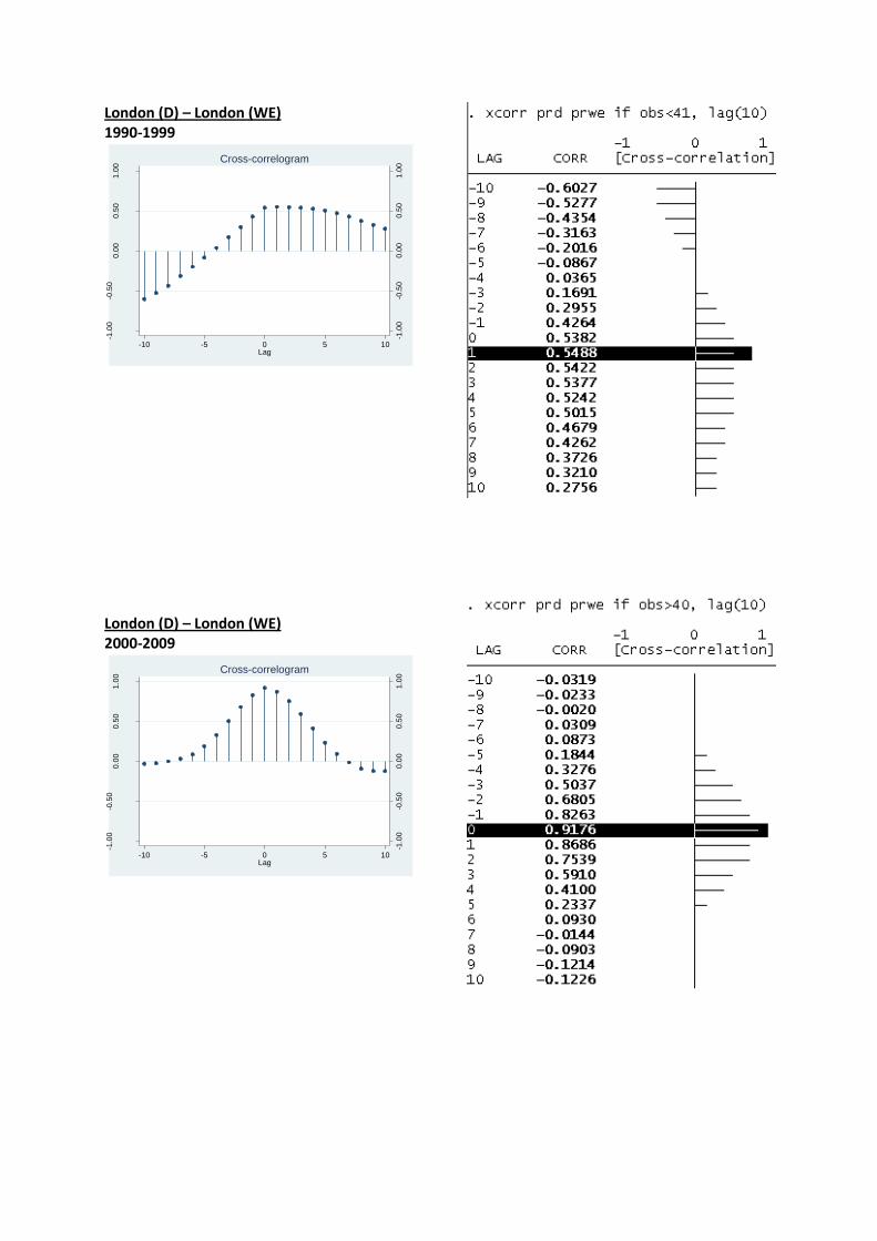
98
London (D) – London (WE) 1990-1999
London (D) – London (WE) 2000-2009
-1.0
0-0
.50
0.0
00
.50
1.0
0
-1.0
0-0
.50
0.0
00
.50
1.0
0
Cro
ss-c
orr
ela
tio
ns o
f p
rd a
nd p
rwe
-10 -5 0 5 10Lag
Cross-correlogram
-1.0
0-0
.50
0.0
00
.50
1.0
0
-1.0
0-0
.50
0.0
00
.50
1.0
0
Cro
ss-c
orr
ela
tio
ns o
f p
rd a
nd p
rwe
-10 -5 0 5 10Lag
Cross-correlogram

99
London (LC) – London (WE) 1990-1999
London (LC) – London (WE) 2000-2009
-1.0
0-0
.50
0.0
00
.50
1.0
0
-1.0
0-0
.50
0.0
00
.50
1.0
0
Cro
ss-c
orr
ela
tio
ns o
f p
rlc a
nd p
rwe
-10 -5 0 5 10Lag
Cross-correlogram
-1.0
0-0
.50
0.0
00
.50
1.0
0
-1.0
0-0
.50
0.0
00
.50
1.0
0
Cro
ss-c
orr
ela
tio
ns o
f p
rlc a
nd p
rwe
-10 -5 0 5 10Lag
Cross-correlogram

100
Average and Asking Rent (AR):
London (D) – London (LC) 1990-1999
London (D) – London (LC) 2000-2009
-1.0
0-0
.50
0.0
00
.50
1.0
0
-1.0
0-0
.50
0.0
00
.50
1.0
0
Cro
ss-c
orr
ela
tio
ns o
f a
rd a
nd a
rlc
-10 -5 0 5 10Lag
Cross-correlogram
-1.0
0-0
.50
0.0
00
.50
1.0
0
-1.0
0-0
.50
0.0
00
.50
1.0
0
Cro
ss-c
orr
ela
tio
ns o
f a
rd a
nd a
rlc
-10 -5 0 5 10Lag
Cross-correlogram

101
London (D) – London (WE) 1990-1999
London (D) – London (WE) 2000-2009
-1.0
0-0
.50
0.0
00
.50
1.0
0
-1.0
0-0
.50
0.0
00
.50
1.0
0
Cro
ss-c
orr
ela
tio
ns o
f a
rd a
nd a
rwe
-10 -5 0 5 10Lag
Cross-correlogram
-1.0
0-0
.50
0.0
00
.50
1.0
0
-1.0
0-0
.50
0.0
00
.50
1.0
0
Cro
ss-c
orr
ela
tio
ns o
f a
rd a
nd a
rwe
-10 -5 0 5 10Lag
Cross-correlogram

102
London (LC) – London (WE) 1990-1999
London (LC) – London (WE) 2000-2009
-1.0
0-0
.50
0.0
00
.50
1.0
0
-1.0
0-0
.50
0.0
00
.50
1.0
0
Cro
ss-c
orr
ela
tio
ns o
f a
rlc a
nd a
rwe
-10 -5 0 5 10Lag
Cross-correlogram
-1.0
0-0
.50
0.0
00
.50
1.0
0
-1.0
0-0
.50
0.0
00
.50
1.0
0
Cro
ss-c
orr
ela
tio
ns o
f a
rlc a
nd a
rwe
-10 -5 0 5 10Lag
Cross-correlogram

103
Vacancy: London (D) – London (LC) 1990-1999
London (D) – London (LC) 2000-2009
-1.0
0-0
.50
0.0
00
.50
1.0
0
-1.0
0-0
.50
0.0
00
.50
1.0
0
Cro
ss-c
orr
ela
tio
ns o
f va
can
cyd a
nd v
aca
ncylc
-10 -5 0 5 10Lag
Cross-correlogram
-1.0
0-0
.50
0.0
00
.50
1.0
0
-1.0
0-0
.50
0.0
00
.50
1.0
0
Cro
ss-c
orr
ela
tio
ns o
f va
can
cyd a
nd v
aca
ncylc
-10 -5 0 5 10Lag
Cross-correlogram

104
London (D) – London (WE) 1990-1999
London (D) – London (WE) 2000-2009
-1.0
0-0
.50
0.0
00
.50
1.0
0
-1.0
0-0
.50
0.0
00
.50
1.0
0
Cro
ss-c
orr
ela
tio
ns o
f va
can
cyd a
nd v
aca
ncyw
e
-10 -5 0 5 10Lag
Cross-correlogram
-1.0
0-0
.50
0.0
00
.50
1.0
0
-1.0
0-0
.50
0.0
00
.50
1.0
0
Cro
ss-c
orr
ela
tio
ns o
f va
can
cyd a
nd v
aca
ncyw
e
-10 -5 0 5 10Lag
Cross-correlogram

105
London (LC ) – London (WE) 1990-1999
London (LC) – London (WE) 2000-2009
-1.0
0-0
.50
0.0
00
.50
1.0
0
-1.0
0-0
.50
0.0
00
.50
1.0
0
Cro
ss-c
orr
ela
tio
ns o
f va
can
cylc
an
d v
aca
ncyw
e
-10 -5 0 5 10Lag
Cross-correlogram
-1.0
0-0
.50
0.0
00
.50
1.0
0
-1.0
0-0
.50
0.0
00
.50
1.0
0
Cro
ss-c
orr
ela
tio
ns o
f va
can
cylc
an
d v
aca
ncyw
e
-10 -5 0 5 10Lag
Cross-correlogram

106
Yield: London (D) – London (LC) 1990-1999
London (D) – London (LC) 2000-2009
-1.0
0-0
.50
0.0
00
.50
1.0
0
-1.0
0-0
.50
0.0
00
.50
1.0
0
Cro
ss-c
orr
ela
tio
ns o
f yie
ldd
and
yie
ldlc
-10 -5 0 5 10Lag
Cross-correlogram
-1.0
0-0
.50
0.0
00
.50
1.0
0
-1.0
0-0
.50
0.0
00
.50
1.0
0
Cro
ss-c
orr
ela
tio
ns o
f yie
ldd
and
yie
ldlc
-10 -5 0 5 10Lag
Cross-correlogram

107
London (D) – London (WE) 1990-1999
London (D) – London (WE) 2000-2009
-1.0
0-0
.50
0.0
00
.50
1.0
0
-1.0
0-0
.50
0.0
00
.50
1.0
0
Cro
ss-c
orr
ela
tio
ns o
f yie
ldd
and
yie
ldw
e
-10 -5 0 5 10Lag
Cross-correlogram
-1.0
0-0
.50
0.0
00
.50
1.0
0
-1.0
0-0
.50
0.0
00
.50
1.0
0
Cro
ss-c
orr
ela
tio
ns o
f yie
ldd
and
yie
ldw
e
-10 -5 0 5 10Lag
Cross-correlogram

108
London (LC ) – London (WE) 1990-1999
London (LC) – London (WE) 2000-2009
-1.0
0-0
.50
0.0
00
.50
1.0
0
-1.0
0-0
.50
0.0
00
.50
1.0
0
Cro
ss-c
orr
ela
tio
ns o
f yie
ldlc
and
yie
ldw
e
-10 -5 0 5 10Lag
Cross-correlogram
-1.0
0-0
.50
0.0
00
.50
1.0
0
-1.0
0-0
.50
0.0
00
.50
1.0
0
Cro
ss-c
orr
ela
tio
ns o
f yie
ldlc
and
yie
ldw
e
-10 -5 0 5 10Lag
Cross-correlogram

109
* 3. Business Cycle correlation *3.1 Global correlation
RENTS Prime Rents (PR): Stockholm – London (LC) Economic decline (= 0)
Stockholm – London (LC) Upswing (= 1)
-1.0
0-0
.50
0.0
00
.50
1.0
0
-1.0
0-0
.50
0.0
00
.50
1.0
0
Cro
ss-c
orr
ela
tio
ns o
f p
rs a
nd
prlc
-4 -2 0 2 4Lag
Cross-correlogram
-1.0
0-0
.50
0.0
00
.50
1.0
0
-1.0
0-0
.50
0.0
00
.50
1.0
0
Cro
ss-c
orr
ela
tio
ns o
f p
rs a
nd
prlc
-4 -2 0 2 4Lag
Cross-correlogram

110
Average/Asking Rents (AR): Stockholm – London (LC) Economic decline (= 0)
Stockholm – London (LC) Upswing (= 1)
-1.0
0-0
.50
0.0
00
.50
1.0
0
-1.0
0-0
.50
0.0
00
.50
1.0
0
Cro
ss-c
orr
ela
tio
ns o
f a
rs a
nd
arlc
-4 -2 0 2 4Lag
Cross-correlogram
-1.0
0-0
.50
0.0
00
.50
1.0
0
-1.0
0-0
.50
0.0
00
.50
1.0
0
Cro
ss-c
orr
ela
tio
ns o
f a
rs a
nd
arlc
-4 -2 0 2 4Lag
Cross-correlogram

111
Stockholm – New York Economic decline (= 0)
Stockholm – New York Upswing (= 1)
-1.0
0-0
.50
0.0
00
.50
1.0
0
-1.0
0-0
.50
0.0
00
.50
1.0
0
Cro
ss-c
orr
ela
tio
ns o
f a
rs a
nd
arn
y
-4 -2 0 2 4Lag
Cross-correlogram
-1.0
0-0
.50
0.0
00
.50
1.0
0
-1.0
0-0
.50
0.0
00
.50
1.0
0
Cro
ss-c
orr
ela
tio
ns o
f a
rs a
nd
arn
y
-4 -2 0 2 4Lag
Cross-correlogram

112
London (LC) – New York Economic decline (= 0)
London (LC) – New York Upswing (= 1)
-1.0
0-0
.50
0.0
00
.50
1.0
0
-1.0
0-0
.50
0.0
00
.50
1.0
0
Cro
ss-c
orr
ela
tio
ns o
f a
rlc a
nd a
rny
-2 -1 0 1 2Lag
Cross-correlogram
-1.0
0-0
.50
0.0
00
.50
1.0
0
-1.0
0-0
.50
0.0
00
.50
1.0
0
Cro
ss-c
orr
ela
tio
ns o
f a
rlc a
nd a
rny
-2 -1 0 1 2Lag
Cross-correlogram

113
Vacancy: Stockholm – London (LC) Economic decline (= 0)
Stockholm – London (LC) Upswing (= 1)
-1.0
0-0
.50
0.0
00
.50
1.0
0
-1.0
0-0
.50
0.0
00
.50
1.0
0
Cro
ss-c
orr
ela
tio
ns o
f va
can
cys a
nd
va
can
cylc
-4 -2 0 2 4Lag
Cross-correlogram
-1.0
0-0
.50
0.0
00
.50
1.0
0
-1.0
0-0
.50
0.0
00
.50
1.0
0
Cro
ss-c
orr
ela
tio
ns o
f va
can
cys a
nd
va
can
cylc
-4 -2 0 2 4Lag
Cross-correlogram

114
Stockholm – New York Economic decline (= 0)
Stockholm – New York Upswing (= 1)
-1.0
0-0
.50
0.0
00
.50
1.0
0
-1.0
0-0
.50
0.0
00
.50
1.0
0
Cro
ss-c
orr
ela
tio
ns o
f va
can
cys a
nd
va
can
cyny
-4 -2 0 2 4Lag
Cross-correlogram
-1.0
0-0
.50
0.0
00
.50
1.0
0
-1.0
0-0
.50
0.0
00
.50
1.0
0
Cro
ss-c
orr
ela
tio
ns o
f va
can
cys a
nd
va
can
cyny
-4 -2 0 2 4Lag
Cross-correlogram

115
London (LC) – New York Economic decline (= 0)
London (LC)– New York Upswing (= 1)
-1.0
0-0
.50
0.0
00
.50
1.0
0
-1.0
0-0
.50
0.0
00
.50
1.0
0
Cro
ss-c
orr
ela
tio
ns o
f va
can
cylc
an
d v
aca
ncyn
y
-4 -2 0 2 4Lag
Cross-correlogram
-1.0
0-0
.50
0.0
00
.50
1.0
0
-1.0
0-0
.50
0.0
00
.50
1.0
0
Cro
ss-c
orr
ela
tio
ns o
f va
can
cylc
an
d v
aca
ncyn
y
-4 -2 0 2 4Lag
Cross-correlogram

116
Yield: Stockholm – London (LC) Economic decline (= 0)
Stockholm – London (LC) Upswing (= 1)
-1.0
0-0
.50
0.0
00
.50
1.0
0
-1.0
0-0
.50
0.0
00
.50
1.0
0
Cro
ss-c
orr
ela
tio
ns o
f yie
lds a
nd y
ield
lc
-4 -2 0 2 4Lag
Cross-correlogram
-1.0
0-0
.50
0.0
00
.50
1.0
0
-1.0
0-0
.50
0.0
00
.50
1.0
0
Cro
ss-c
orr
ela
tio
ns o
f yie
lds a
nd y
ield
lc
-4 -2 0 2 4Lag
Cross-correlogram

117
Stockholm – New York Economic decline (= 0)
Stockholm – New York Upswing (= 1)
-1.0
0-0
.50
0.0
00
.50
1.0
0
-1.0
0-0
.50
0.0
00
.50
1.0
0
Cro
ss-c
orr
ela
tio
ns o
f yie
lds a
nd y
ield
nyc
-4 -2 0 2 4Lag
Cross-correlogram
-1.0
0-0
.50
0.0
00
.50
1.0
0
-1.0
0-0
.50
0.0
00
.50
1.0
0
Cro
ss-c
orr
ela
tio
ns o
f yie
lds a
nd y
ield
nyc
-4 -2 0 2 4Lag
Cross-correlogram

118
London (LC) – New York Economic decline (= 0)
London (LC)– New York Upswing (= 1)
-1.0
0-0
.50
0.0
00
.50
1.0
0
-1.0
0-0
.50
0.0
00
.50
1.0
0
Cro
ss-c
orr
ela
tio
ns o
f yie
ldlc
and
yie
ldn
yc
-4 -2 0 2 4Lag
Cross-correlogram
-1.0
0-0
.50
0.0
00
.50
1.0
0
-1.0
0-0
.50
0.0
00
.50
1.0
0
Cro
ss-c
orr
ela
tio
ns o
f yie
ldlc
and
yie
ldn
yc
-4 -2 0 2 4Lag
Cross-correlogram

119
*3.2 Local/Domestic Correlation
Rents
Prime Rents (PR): London (D) – London (LC) Economic decline (= 0)
London (D) – London (LC) Upswing (= 1)
-1.0
0-0
.50
0.0
00
.50
1.0
0
-1.0
0-0
.50
0.0
00
.50
1.0
0
Cro
ss-c
orr
ela
tio
ns o
f p
rd a
nd p
rlc
-4 -2 0 2 4Lag
Cross-correlogram
-1.0
0-0
.50
0.0
00
.50
1.0
0
-1.0
0-0
.50
0.0
00
.50
1.0
0
Cro
ss-c
orr
ela
tio
ns o
f p
rd a
nd p
rlc
-4 -2 0 2 4Lag
Cross-correlogram

120
London (D) – London (WE) Economic decline (= 0)
London (D) – London (WE) Upswing (= 1)
-1.0
0-0
.50
0.0
00
.50
1.0
0
-1.0
0-0
.50
0.0
00
.50
1.0
0
Cro
ss-c
orr
ela
tio
ns o
f p
rd a
nd p
rwe
-4 -2 0 2 4Lag
Cross-correlogram
-1.0
0-0
.50
0.0
00
.50
1.0
0
-1.0
0-0
.50
0.0
00
.50
1.0
0
Cro
ss-c
orr
ela
tio
ns o
f p
rd a
nd p
rwe
-4 -2 0 2 4Lag
Cross-correlogram

121
London (LC) – London (WE) Economic decline (= 0)
London (LC) – London (WE) Upswing (= 1)
-1.0
0-0
.50
0.0
00
.50
1.0
0
-1.0
0-0
.50
0.0
00
.50
1.0
0
Cro
ss-c
orr
ela
tio
ns o
f p
rlc a
nd p
rwe
-4 -2 0 2 4Lag
Cross-correlogram
-1.0
0-0
.50
0.0
00
.50
1.0
0
-1.0
0-0
.50
0.0
00
.50
1.0
0
Cro
ss-c
orr
ela
tio
ns o
f p
rlc a
nd p
rwe
-4 -2 0 2 4Lag
Cross-correlogram

122
Average/Asking Rents (AR): London (D) – London (LC) Economic decline (= 0)
London (D) – London (LC) Upswing (= 1)
-1.0
0-0
.50
0.0
00
.50
1.0
0
-1.0
0-0
.50
0.0
00
.50
1.0
0
Cro
ss-c
orr
ela
tio
ns o
f a
rd a
nd a
rlc
-4 -2 0 2 4Lag
Cross-correlogram
-1.0
0-0
.50
0.0
00
.50
1.0
0
-1.0
0-0
.50
0.0
00
.50
1.0
0
Cro
ss-c
orr
ela
tio
ns o
f a
rd a
nd a
rlc
-4 -2 0 2 4Lag
Cross-correlogram

123
London (D) – London (WE) Economic decline (= 0)
London (D) – London (WE) Upswing (= 1)
-1.0
0-0
.50
0.0
00
.50
1.0
0
-1.0
0-0
.50
0.0
00
.50
1.0
0
Cro
ss-c
orr
ela
tio
ns o
f a
rd a
nd a
rwe
-4 -2 0 2 4Lag
Cross-correlogram
-1.0
0-0
.50
0.0
00
.50
1.0
0
-1.0
0-0
.50
0.0
00
.50
1.0
0
Cro
ss-c
orr
ela
tio
ns o
f a
rd a
nd a
rwe
-4 -2 0 2 4Lag
Cross-correlogram

124
London (LC) – London (WE) Economic decline (= 0)
London (LC) – London (WE) Upswing (= 1)
-1.0
0-0
.50
0.0
00
.50
1.0
0
-1.0
0-0
.50
0.0
00
.50
1.0
0
Cro
ss-c
orr
ela
tio
ns o
f a
rlc a
nd a
rwe
-4 -2 0 2 4Lag
Cross-correlogram
-1.0
0-0
.50
0.0
00
.50
1.0
0
-1.0
0-0
.50
0.0
00
.50
1.0
0
Cro
ss-c
orr
ela
tio
ns o
f a
rlc a
nd a
rwe
-4 -2 0 2 4Lag
Cross-correlogram

125
Vacancy: London (D) – London (LC) Economic decline (= 0)
Vacancy: London (D) – London (LC) Upswing (= 1)
-1.0
0-0
.50
0.0
00
.50
1.0
0
-1.0
0-0
.50
0.0
00
.50
1.0
0
Cro
ss-c
orr
ela
tio
ns o
f va
can
cyd a
nd v
aca
ncylc
-4 -2 0 2 4Lag
Cross-correlogram
-1.0
0-0
.50
0.0
00
.50
1.0
0
-1.0
0-0
.50
0.0
00
.50
1.0
0
Cro
ss-c
orr
ela
tio
ns o
f va
can
cyd a
nd v
aca
ncylc
-4 -2 0 2 4Lag
Cross-correlogram

126
London (D) – London (WE) Economic decline (= 0)
London (D) – London (WE) Upswing (= 1)
-1.0
0-0
.50
0.0
00
.50
1.0
0
-1.0
0-0
.50
0.0
00
.50
1.0
0
Cro
ss-c
orr
ela
tio
ns o
f va
can
cyd a
nd v
aca
ncyw
e
-4 -2 0 2 4Lag
Cross-correlogram
-1.0
0-0
.50
0.0
00
.50
1.0
0
-1.0
0-0
.50
0.0
00
.50
1.0
0
Cro
ss-c
orr
ela
tio
ns o
f va
can
cyd a
nd v
aca
ncyw
e
-4 -2 0 2 4Lag
Cross-correlogram

127
London (LC) – London (WE) Economic decline (= 0)
London (LC) – London (WE) Upswing (= 1)
-1.0
0-0
.50
0.0
00
.50
1.0
0
-1.0
0-0
.50
0.0
00
.50
1.0
0
Cro
ss-c
orr
ela
tio
ns o
f va
can
cylc
an
d v
aca
ncyw
e
-4 -2 0 2 4Lag
Cross-correlogram
-1.0
0-0
.50
0.0
00
.50
1.0
0
-1.0
0-0
.50
0.0
00
.50
1.0
0
Cro
ss-c
orr
ela
tio
ns o
f va
can
cylc
an
d v
aca
ncyw
e
-4 -2 0 2 4Lag
Cross-correlogram

128
Yield: London (D) – London (LC) Economic decline (= 0)
London (D) – London (LC) Upswing (= 1)
-1.0
0-0
.50
0.0
00
.50
1.0
0
-1.0
0-0
.50
0.0
00
.50
1.0
0
Cro
ss-c
orr
ela
tio
ns o
f yie
ldd
and
yie
ldlc
-4 -2 0 2 4Lag
Cross-correlogram
-1.0
0-0
.50
0.0
00
.50
1.0
0
-1.0
0-0
.50
0.0
00
.50
1.0
0
Cro
ss-c
orr
ela
tio
ns o
f yie
ldd
and
yie
ldlc
-4 -2 0 2 4Lag
Cross-correlogram

129
London (D) – London (WE) Economic decline (= 0)
London (D) – London (WE) Upswing (= 1)
-1.0
0-0
.50
0.0
00
.50
1.0
0
-1.0
0-0
.50
0.0
00
.50
1.0
0
Cro
ss-c
orr
ela
tio
ns o
f yie
ldd
and
yie
ldw
e
-4 -2 0 2 4Lag
Cross-correlogram
-1.0
0-0
.50
0.0
00
.50
1.0
0
-1.0
0-0
.50
0.0
00
.50
1.0
0
Cro
ss-c
orr
ela
tio
ns o
f yie
ldd
and
yie
ldw
e
-4 -2 0 2 4Lag
Cross-correlogram

130
London (LC) – London (WE) Economic decline (= 0)
London (LC) – London (WE) Upswing (= 1)
-1.0
0-0
.50
0.0
00
.50
1.0
0
-1.0
0-0
.50
0.0
00
.50
1.0
0
Cro
ss-c
orr
ela
tio
ns o
f yie
ldlc
and
yie
ldw
e
-4 -2 0 2 4Lag
Cross-correlogram
-1.0
0-0
.50
0.0
00
.50
1.0
0
-1.0
0-0
.50
0.0
00
.50
1.0
0
Cro
ss-c
orr
ela
tio
ns o
f yie
ldlc
and
yie
ldw
e
-4 -2 0 2 4Lag
Cross-correlogram