Embed Size (px)
Citation preview

This PDF is a selection from an out-of-print volume from the NationalBureau of Economic Research
Volume Title: The Role of the Computer in Economic and Social Researchin Latin America
Volume Author/Editor: Nancy D. Ruggles, ed.
Volume Publisher: NBER
Volume ISBN: 0-87014-260-7
Volume URL: http://www.nber.org/books/rugg75-1
Publication Date: 1975
Chapter Title: Macroeconomic Model Building in Latin America: TheMexican Case
Chapter Author: Abel Beltran del Rio, Lawrence R. Klein
Chapter URL: http://www.nber.org/chapters/c3772
Chapter pages in book: (p. 161 - 190)

MACROECONOMETRIC MODEL BUILDING IN LATIN AMERICA:THE MEXICAN CASE
ABEL BELTRAN DEL Rio AND LAWRENCE R. KLEINWharton Econometric Forecasting Associates, Inc.*
1. INTRODUCTION
Wairas' great vision of describing mathematically the functioning of a completeeconomy has been realized in our time.' With the advent of social accounting,the Keynesian macroeconomic shortcut, and the computer, the construction ofbig mathematico-statistical representations of national economies has been madepossible. The first macroeconomic models appeared during the 1930s and 1940sas descriptions of the advanced economies. The models of the developing economiesbegan appearing during the 1950s, but it was not until the second half of the1960s that macromodels were constructed for the Latin American economies.Since then, they have proliferated rapidly.
At the beginning, some of the macroeconometric models for developingeconomies did not differ much from those of the mature, industrialized economies.Their general structure and the specification of the individual equations wassimilar, if not identical, to the pioneer models. This is perfectly understandable.However, the usefulness of these models for alternative policy simulations orforecasting was limited. They were not faithful representations of their economiesand could not be expected to follow their movements very closely.
More recently, however, stimulated by the post-Keynesian theorizing oneconomic growth and development, and by the efforts of econometricians totailor their models better to the features of each country, the LDC models havebegun to differ from those of the advanced economies. The differences intend torepresent variety in economic development, behavior, technology, and institutionsthat characterize the developing economies, as well as the economic peculiarities ofthe country in question. This does not mean that. the structure and specificationof the LDC models are (or are expected to be) totally different from those of theadvanced nations. After all, the anatomy and physiology of all economies areessentially the same. The difference seems to be in size, complexity, refinement ofmarket mechanism, and speed with which the macroeconomic organs function,using as the standard of comparison those of the advanced economies. Macro
* The research of the Mexican Department (DIEMEX) of Wharton EFA is sponsored by thefollowing institutions: Banco Interamericano de Desarrollo; Banco Nacional de Comercio Exterior.S.A.; Banco Nacional de Mexico, S.A.; Celanese Mexicana, S.A.; Cerveceria Cuauhtemoc, S.A,;Conductores Monterrey, S.A.; Credito Mexicano, S.A.; Du Pont, S.A. de C.V.; Financiera. Acepta-ciones, S.A.; Financiera del Norte, S.A.; Grupo Cydsa, S.A.; Hojalata y Lamina, S.A.; I.B.M: deMexico, S.A.; Instituto Nacional de Planificacion de Ia Republica Peruana; Interamericana deArrendamientos, S.A.; Manufacturera Corpomex. S.A.; Nacional Financiera. S.A.; Procesos ySistemas, S.A.; Representaciones Generales, S.A.; Tecnica Industrial, S.A.; Tesoreria del Etado deChihuahua; Troqueles y Esmaltes, S.A.; Valores Industriates. S.A.
Walras had a micro vision modern econometric models have been aggregative. The basicprinciple, however, is the same in both cases, and modern models are now moving strongly in a micro-economic direction.

162 Economic and Social Research in Latin America
bottlenecks, which are most useful for econometric specifications, appear indifferent parts of the system—agriculture being a typical example. Latin Americanmodels, being the last to appear so far, have received the benefits of these effortsfor more faithful econometric portrayal.
The purpose of this paper is to present the Mexican econometric model thatwe have developed at the Department of Econometric Research on Mexico ofWharton EFA2 and to make some general comments on econometric modelbuilding for the developing economies. Applications of the Mexican model willalso be included.
2. SOME PRELIMINARY CONSIDERATIONS OF MODEL BUILDING FORTHE DEVELOPING EcoNoMIEs
The best procedure for model specification of developing economies is to tryto translate into econometrics their characteristic features. These have beenelaborated extensively by the development theorists in their efforts to distinguishconceptually the LDC from the MDC.3 A brief listing and discussion of thesedistinctive traits seem a natural way to start. This list can be considered as a kindof descriptive model, or standard, which should help in the specification of theMexican model, and in evaluating the specifications of other macroeconometricmodels of developing economies in which we may be interested. For this reason,the list will be supplemented with some features peculiar to the Latin Americaneconomies and, particularly, to the Mexican economy.
Since the differences between the LDC and the MDC arise from their relativeposition in the development race, all of the traits listed are also present, in somedegree, in the advanced countries. That is why there is a fundamental similarityin the models of both kinds of economies. Moreover, social accounting systems,whose entries are to be explained by macromodels, are essentially the same inlayout for all market economies. This is a recognition not only of the basic under-lying similarity between the LDC and the MDC, but also of the accounting sourceof similarity between their models. Accordingly, both types of macromodelsattempt, with their equations, to explain consumption, investment, exports,imports, production, prices, and sO on. Consequently, the differences which we arelisting below should be seen as traits that are only more apparent and pronouncedin the LDC but not totally absent in the MDC. However, they do call for differencesin the models, through endogenization of some variables, or through new, specialequations, or through different specifications for the common ones.
In the list that follows, two related features of the developing economies,one external, the other internal, seem to be dominant: (1) their comparativeoverall productive backwardness vis-à-vis the MDC, and (2) the relative uneven-ness of their productive sectors, when compared internally. In the literature, (1)
of the main purposes of this department (DIEMEX) has been to determine the extent towhich econometric tools can be applied to developing countries. The cases of Mexico and Peru havebeen explored so far.
take these common abbreviations, less developed (LDC) and more developed country(MDC). from the development literature. See, for example, E. E. Hagen, The Economics of Development(Homewood, Ill.: Irwin, 1968), p. 6. By an LDC, we understand here an economy in transition, activein the process of growth, not a stationary one.

Macroeconometric Model Building in Latin America 163
has also been called supply deficiency, output constraint, technological backward-ness, and so forth, (2) has been called "dualism," sectoral gaps, traditional versusmodern sectotS, agricultural versus industrial sectors, regional or structuralimbalance, and so on. Most of the other features and problems of the developingeconomies seem to arise from these two. The external problems of capital andtechnological imports, exports of primary goods, balance-of-payments problems,as well as the internal problems of maldistribution of income, rural-urban labormigration, the big economic role of the government, existence of overcapacity inthe modern productive sectors, and in some cases, even inflation, can be traced tothem.
Supply Deficiency
If we take the Keynesian view that the main characteristic of industrializednations is their possession of a developed and efficient productive sector, and thattheir short-run problem is the recurrent deficiency in aggregate demand, we cansay, by contrast, that the main trait of developing countries is their comparativedeficiency in aggregate supply.4 Agricultural supply, still bound to old-fashionedproductive methods, is very much the result of the whims of the weather. Industryis relatively underdeveloped, concentrated on a few products (automobiles andsteel are the favorites in Latin America), subject to bottlenecks in physical (rawmaterials or machinery) or technological (operative know-how, organizationalknowledge) inputs, and likely to be affected by political events. Services are com-paratively small, hampered, too, by lack of skilled technicians and adequatecapital equipment.
This does not mean that the developing countries have no short-run problemof aggregate demand. They do, and they need the Keynesian tools to keep theirexisting productive capacity as fully utilized as possible, without undue inflationarypressure. However, their crucial problem is to enlarge that productive capacityin order to make employment, income, and demand possible. They have beforethem the example of the MDC and of recent productive successes, like Russiaand Japan. Internal social demands arising from growing expectations also con-tribute to making supply enlargement their basic economic concern.
The process of economic growth, then, is central in the developing economies,and it should be captured in their economic descriptions. Other characteristicsand processes are, one way or another, connected with growth. Those connec-tions should be given special importance in model building. Growth of inputs,especially capital, which is the bottleneck in developing economies, should begiven special attention. Labor migration from the rural to the urban productivesector should also be considered. By the same token, the determinants or majorconstraints of these capacity-enlarging inputs, normally frozen into the assump-tions of the short run, should be examined and made to play their part, if possible,in the main process of development.
Keynesian problem was why factories and machines shut down in a rich country or theparadox of poverty in the midst of plenty. The developing nations problem is how to bring machinesand factories to the country or how to break the ancestral condition of poverty by importing superiorproductive methods.

164 Economic and Social Research in Latin America
Besides, the actual duration of the "long-run" process of growth of the LDChas been reduced substantially when compared with that of the MDC. The formerare essentially importing from the latter the scientific industrial revolution. Thistakes less time to accomplish. A statistical sample of a decade from an LDC prob-ably compresses growth processes that took from thirty to forty years in theeconomic history of the MDC.
Capital Accumulation and Its Financing
The first binding constraint of development is capital, the nonhuman input.The task of circumventing this bottleneck has become the responsibility of bothprivate and public sectors. Governments of some developing economies havetried not only to provide the capital for infrastructure, but to contribute to theaddition of productive capacity as manufacturers and entrepreneurs. The Mexicaneconomy is a clear example, with its three-hundred "empresas descentralizadas yorganismos de participacion estatal." The Japanese government at the start ofthe big capacity-creating efforts of the Meiji restoration provides another one.5
With the exception of the socialist developing economies, capacity creation,however, has been the responsibility of the private entrepreneur. Private invest-ment has been the larger flow in the accumulation of capital in plant and equip-ment. Public investment, in the form of roads, irrigation projects, communication,and. other infrastructure, has supported these direct productive efforts. Privateand public savings (surplus in current account) have been the sources of financingfunds for the investment flows. The first source, in the LDC especially, has beenexplained as arising from the unequal distribution of income, as we will see below.The second is constrained by the low taxing ability of most of the developingcountries.
Nevertheless, internal savings are not necessarily the first stumbling blockmet by. the LDC in accumulating capital. The lack of enough foreign reserves canbe their binding constraint.6 Since they cannot produce the plant and equipmentnecessary for new industries, capital imports from the MDC become the only wayto grow industrially. Thus, exports and external finances arise as crucial meansof payment for capital accumulation and capacity enlargement.
Exports of Primary Goods
Since agricultural and extractive production are predominant, and manu-factures and services are being developed, the LDC is an exporter of primaryproducts. Its main exports are limited in number and frequently consist of oneor two agricultural or mineral exports. Coffee represents 40 percent and 60 percentof the total merchandise exports of Brazil and Colombia, respectively; sugaraccounts for more than 70 percent of Cuban exports; and copper accounted for76 percent of Chilean goods exports in 1969. Agricultural exports, due to defi-
M. Baba and M. Tatemoto, "Foreign Trade and Economic Growth in Japan: 1858—1937." inEconomic Growth, the Japanese Experience Since the Meyi Era, L. R. Klein and K. Ohkawa, eds.(Homewood, Ill.: Irwin, 1968), p. 169.
H. B. Chenery and M. Strout. "Foreign Assistance and Economic Development." An7ericanEconomic Review, Vol. LV!, No.4, Part 1 (September, 1966), pp. 680—733: or Hagen, op. cit., pp. 366—71.

Macroeconometric Model Building in Latin America 165
ciencies in irrigation infrastructure, ineffective pestilence controls, inadequatefertilizers, and acts of God, are subject to wide fluctuations. In the long run,prices of primary goods are believed to be deteriorating in relationship to theprices of the capacity-creating imports (capital goods and technical services) thatthe LDC need from the MDC.7
The capacity to import, then, of the developing country is constrained to alarge extent by the value of its exports. The analysis and quantification of thisbottleneck is indispensable for the econometric understanding of the develop-mental process. Equally important here isthe transmission of cycles of the MDCto the LDC. To the instability of supply of the primary exports, demand instabilityshould be added. Primary exports depend on the demand-oriented imports of theindustrial countries. Instability in effective demand, the Keynesian problem, isfelt in the export position of the developing countries and is carried through tocapital imports and the expansion of the LDC supply.
External Debt and Foreign Investment
As a corollary of the constraint posed by its export earnings, the developingcountry tends to rely on its capital-account imports to finance its efforts to grow.Normally, this is accomplished by incurring external debt. Debt service increasesas a proportion of export earnings but eventually the added capacity should repayfor itself by increasing exports and/or reducing imports by at least the amount ofdebt and interest incurred.8
Foreign direct investment is the other item of capital account sought by theLDC to finance their capital imports. In spite of its economic advantage in solvingsimultaneously the savings and foreign-currency gaps, foreign investment haspolitical and historical drawbacks (excessive profits, low wages) that limit its use.Some Latin American countries are trying, however, to enlarge it, while legislatingways of reducing its harmful aspects. Recently, in the case of Brazil, large inflowsof foreign investment seem to be one of the main causes of a spectacular increasein the rate of growth. This achievement has been associated with a shift in thecomposition of exports—moving away from traditional goods to manufactures—and has also been associated with a reduction of the rates of inflation.9
Foreign aid, the third element in capital accounts, does not now make asubstantial contribution toward the deficit balance of LDC's current account.Its importance, however, is clear, being a way in which the MDC, or the inter-national organizations supported by them, can perform the function of spreadingtheir technology (or share their productive surpluses) at minimum cost to thedeveloping nations.
'R. Prebisch. "The Economic Development of Latin America and Its Principal Problems."Economic Bulletin for Latin America (February, 1962), pp. 1—22.
8 Hagen. op. cit.. p. 365.° Some writers believe that inflation per se is not the main hindrance to growth. They claim that
the fluctuations in the rate of inflation are the problem. See R. A. Krieger, "Inflation and Growth: theCase of Latin America,' C'olwnbia Journal of World Business, Vol. V. No. 6 (Nov.—Dec. 1970).

166 Economic and Social Research in Latin America
Income Distribution
The characteristic unevenness of the developing economies shows in incomedistribution. The contrast between the "haves" and "have-nots" is more notablein the LDC. It also plays a role in development. Savings and investment are essen-tially done by the recipients of nonwage income. On the other hand, the size ofthe internal market for consumption goods is determined by wage earners. Incomedistribution, then, plays a crucial role in investment and consumption by influenc-ing the flow of internal savings available, while at the same time tending to limitthe size of the internal market for consumption demand. It is also useful in under-standing import substitution in light durable consumer goods, as a commonstrategy of supply enlargement in the LDC.
Population
Rapid population growth can be interpreted as another characteristic of theLDC, resulting from their uneven adoption of modern technique and outlook.Their adoption of modern medicine has substantially reduced the death rate—especially among infants. Birthrates, however, continue at traditionally high levels..Abatement of this condition must await the eventual adoption of values and viewsof the MDC on family size, education of children, and the process of urbanization.Migration, in principle, should also be considered. In most of the Latin Americancountries, however, its role is not significant.
Internal Labor Migration
Internal labor migration is another consequence of the unevenness in theagricultural and industrial sectors in the LDC. Rural labor migration to the citiesis mainly caused by the difference in productivities and wages between thesesectors. In the Mexican case, for example, the ratio of urban-rural labor produc-tivity is approximately 5: 1. Uneven capital accumulation stands at the bottomof the process. A Mexican urban worker has eight times more real capital to workwith than does his rural counterpart. This problem calls for exploration of itsdemographic aspects in order to gain a better understanding of what is involvedfor econometric purposes.
Labor Force and Population
Since models for developing countries should be cast in a long-term frame-work, the growth of human input requires consideration. Enlargement of thelabor force depends on economic and demographic factors. Production functions,converted into labor-requirement functions, and capital-labor ratios have beenused for short-run, demand-oriented determination of employed labor. Populationgrowth, with sex and age composition, are, on the other hand, the long-run supplydeterminants of the working force. In the LDC, the rapid growth of populationmakes the supply approach indispensable. "Development with unlimited suppliesof labor" (and especially when the supply of labor is clearly outmatching theperiodic supply of capital) calls for particular attention on the part of theeconometrician.

Macroeconometric Model Building in Latin America 167
Growth of the skilled and technical part of the labor force is the secondimportant constraint on capacity creation of the LDC in addition to capital.Essentially, this growth is related to education and, particularly, to technologicaleducation. This aspect, so evident and so important, is difficult to introduceexplicitly in statistical models.
Prices, Wages, and Money Supply
Inflation is an unsolved, worldwide problem, but in the developing countries,it appears in its extreme form. Brazil and Chile, with annual price increases of 30percent or more, are two well-known examples. The severity of the problem in theLDC, and especially in Latin America. has had two main explanations in theliterature: (I) structural imbalance in the productive sector (agricultural versusindustrial), and (2) government monetary excesses.1°
However, production bottlenecks, as well as rises in import or export prices,can explain the start, but not the persistence and high rates, of Latin Americanhyperinflations." The prolongation and aggravation of the process requires theaddition of other reinforcing factors, namely excessive growth of the moneysupply, the appearance of the price-wage spiral, and recurrent devaluation. Inother words, structural imbalance can explain inflation; hyperinflation requires amonetary explanation.
Since, generally speaking, organized labor has not been politically independentor strong in Latin America, the price-wage vicious cycle has not been the basicpressuring force. This does not mean that the LDC's unions have not learned fromhyperinflation. They have, but their reactions have, in general, been patient andmodest. In Mexico, for example, they endured substantial real-wage reductionsduring the 1940s and early 1950s. The main fuel, thus, has come from the activityof the government printing presses. This governmental tendency arises fromgrowing deficits caused by lack of taxing power (rooted, in turn, in political weak-ness) and the growing public expenditures required by growth and welfareprograms. The third self-preserving mechanism, periodic devaluation, enters bothas a result and a further cause of the inflationary process. Internal inflation erodesthe capacity to import development goods, the pace of growth is retarded, and adevaluation is in order to move the economy again. This gives a new impetus toinflation and the mechanism of periodic devaluation is incorporated into theprocess.
Overcapacity
A paradox common to the LDC is the existence of particular pockets ofovercapacity in the midst of general supply limitation. It appears essentially in themodern productive sectors, and it can be larger than that of the MDC's corre-sponding sectors. Some examples are the automobile industries in Argentina,Chile, and Mexico; other cases are the Mexican poultry industry and its hotel
• '°These two opposite schools, the structuralists and the monetarists, are very well represented inInflation and Growth in Latin America, W. Baer and I. Kerstenetzky, eds. (Homewood. ill.: Irwin, 1964).
See W. A. Lewis, "Closing Remarks," in Baer and Kerstenetzky, op. cit, p. 24.

168 Economic and Social Research in Latin America
industry.'2 There are several reasons for this: (I) inaccurate demand estimates,due to lack of statistical information or the cost of gathering it; (2) the mirage ofprotectionism and the entrepreneurial desire to control the new market; and (3)the oversized plant and equipment available in the MDC.
Length of Lags
Based on observation of the behavior in the LDC, it seems that the time delays,or lags, between economic impulse and economic reaction differ from those of theMDC. With regard to private consumption, impulsiveness or lack of carefulconsumer planning may very well produce shorter income-consumption lags. Ininvestment, the reverse may be true, because of the much larger construction andinstallation periods. The decision lag is perhaps shorter here, due to lack of longinvestigations and planning, but the implementation lag is certainly longer, evenwhen the smaller size of investment goods in the developing economy is considered.Demographic processes are probably longer, due to poorness of communications,illiteracy, and traditional inertia.
Government and Political Change
The role of the government in the economy is usually bigger in the developingcountry. In most cases, the degree of economic intervention and direct participa-tion in economic life is larger than in the MDC. It is not unusual, then, to find thegovernment of the LDC with more economic instruments at its disposal than itsMDC counterpart has. Also, it is common to find these governments as one of thelarger (if not the largest) of the industrialists or merchants. When this is the case,a cyclical element is introduced in the economy which coincides with the politicalcycle: this arises not only from the stop-and-go nature of government investmentat each administrative change, but also from the impact on private investment,which normally takes a waiting position during political changes.
3. THE MEXICAN MODEL
The Mexican macroeconometric model presented here is the latest one in asuccession of versions developed in an ongoing project of research on Mexico atWharton EFA. This version, V, has been produced by enlargements and modifi-cations of the earlier attempts. The purpose of these additions and changes hasbeen to incorporate successively, as we were able to secure more and better data,additional aspects of the economy, and to respecify equations as we tried toapproximate more closely the actual workings of the economy.
Each successive version was an attempt to make the model closer to what weconsider to be the defining characteristics of the Mexican economy. Owing tolimitations of space, we will not give here a full explanation of the theoretical
12 Out Auto Plants," Business Week. May 22, 1971. p. 36, and "Crecimiento Desor-denado en Ia Industria Avicola," Excelsior, May 9, 1971. A recent general statement of overcapacityin the Mexican economy can be found in A. J. Yarza. "El Futuro del Proceso de Industrializacion enMexico," El Trimestre Economico, No. 151 (July—Sept., 1971), pp. 87—88.

Macroeconometric Model Building in Latin America 169
and institutional justification of the behavioral equations. For that, the inter-ested reader is referred to the full document presented at the Cuernavacaconference. We will, however, list briefly the main features that we have triedto incorporate, which are those of section 2, plus those peculiar to the Mexicaneconomy:
1. Internal and external sources of instability: the impact of the politicalclimate on the economy and the dependence on foreign trade; the internal andexternal sources of inflation.
2. The dominant role played by the federal government as infrastructurebuilder and entrepreneur; public finances.
3. The general unevenness in economic life as exemplified in functionalincome distribution, in rural versus urban production, in federal versus non-federal taxation.
4. The rapid demographic processes resulting in high population growth,urbanization, or rural-urban labor-force migration.
5. The proximity to the U.S. markets with its. effects on international labormigration, tourism and border transactions, and trade in general.
6. The development process of creating capacity, through capital and tech-nological imports, in the context of general capital limitations and abundance ofunskilled and semiskilled labor.
7. The comparatively shorter decision-making horizon in all economicprocesses, resulting in shorter lags vis-à-vis the MDC.
8. The simplicity of economic organisms and behavior when compared withthose of the MDC.
The rest of this section consists of the nomenclature and the full listing of theequations of the model. The list contains 143 equations, 40 of which are behavioral;the rest are accounting and other identities. The behavioral equations have beenestimated by the ordinary least squares method; the 10 containing distributed lagswere estimated by fitting a polynomial of third degree with two end-pointrestrictions.
We list now alphabetically the symbols used and their meanings. The symbolsare of two kinds: simple (consisting of only one letter) and compound (consistingof two or more letters and numbers). In the case of the compound symbols, thefinal letters and numbers have the following meaning:
Ending in C Current billion pesosEnding in R Real billion pesos of 1950Ending in DC Current billion dollarsEnding in L Per worker of the productive sector in questionEnding in N Per capitaEnding in % Annual rate of change -Ending in 1, 2, or 3 Lags of one, two, or three previous yearsAll predetermined variables (exogenous or lagged endogenous) are underlined.
The only exceptions to these rules are two compound symbols: LI and L23, ruraland urban labor force. The number endings here do not mean lags, but primaryand secondary plus tertiary productive sectors, respectively. They are not, thus,underlined. The abbreviations NIA and BOP mean National Income Accountsand Balance of Payment Account.

170 Economic and Social Research in Latin America
A condensed flow chart of this model and, in fact, a very condensed versionof this whole paper, can be found in Abel Beltran del Rio, "Mexico: an Economyat the Crossroads," Wharton Quarterly, University of Pennsylvania, Fall 1971.
LIST OF VARIABLES
B
Balance of productive factors in NIABalance of productive factors in BOPBalance of goods in BOPBalance of goods, services and factors or net foreign demand in NIABalance of goods, services and factors or net foreign demand in BOPBalance of goods, tourism and border transactions in NIABalance of goods, tourism and border transactions in BOPBalance of other items in current account in BOPBalance of tourism and border transactions in BOP
CPublic consumptionDomestic or internal aggregate demandCapacity to import or current earnings deflated by import price-indexCOCOP multiplied by DUMRS
_______
Domestic, physical consumption of copper (millions of tons)
_______
Domestic, physical consumption of cotton (millions of bales)
_______
Domestic, physical consumption of lead (millions of tons)Domestic, physical consumption of nonferrous metals: lead, copper and zinc (millions
of tons)Private consumptionPrivate consumption per capita (thousands of 1950 pesos per person)Consumption
D
________
Public external debtPublic external debtDepreciationChange in public external debtChange in gross domestic productPublic depreciationDisposable personal income per capita (thousands of 1950 pesos per person)
_______
Disposable personal income in the U.S.Disposable personal income in the U.S.Change in export price index, PEUEJ, of main exporting countries to MexicoChange in GNP price deflatorPrivate depreciationDepreciationDummy for government restrictions to the bracero 1.0 for 1965—1968; 0.0
elsewhereDUMCU Dummy for U.S.' suspension of sugar buying from Cuba; 1.0 for 1960—1968; 0.0
elsewhere
________
Dummy for aftereffects of devaluation of 1954; 1.0 for 1956—1961 ; 0.0 elsewhereDummy for political change in Mexico: presidential transitions and other major
political events; 1.0 for 1952—1953. 1958—1959, 1964—1965, and 1961—1963; 0.0elsewhere
_______
Dummy for census revisions of labor data; 1.0 for 1960—1968; 0.0 elsewhere.Dummy for U.S.' trade protection to its nonferrous metal producers; 1.0 for 1958—1968:
0.0 elsewhereDummy for exceptional federal exports tax collection; 1.0 for 1955—1956, 1961, and
1967; 0.0 elsewhere
BFRBFR*BGR
BGSFRBGSFR*
BGSRBGSRBOTRBTBR
CGRCITRCMC
COCDIJCo COPco-COTCOLEACOMET
CPRCPRN
CR
DBGEDCDBGER
DCDDBGRDGDPR
DGRDIPRNDIUDC
DIURDPEUEJDPGNP
DPRDR
DUMBR
DUMDVDUMPO
DUMREDUMRS
DUMTFE

Macroeconometric Model Building in Latin America 171
DUMTPC Dummy for exceptional federal nontax collection; 1.0 for 1965; 0.0 elsewhereDUX23P Change in idle urban productive capacityDXI PRU Change in rural potential population productivityDX23 I P Gaps between urban and rural potential population productivity
E
E4ADC Net production of gold and silverEAAR Net production of gold and silverEAGR Main agricultural goods exports: cotton, coffee and sugarEBRR Labor exports or bracero earnings
EBRRL Labor exports or bracero earnings per Mexican worker (thousands of 1950 pesos perworker)
ECOFR Exports of coffeeECOPR Exports of copperECO TR Exports of cotton
EGC Goods or merchandise exportsEGDC Goods or merchandise exportsEGER Goods exports, explained by equations in the model
EGMFR Manufactured goods exportsEGR Goods or merchandise exports
EGSFR Exports of goods, services and factors or total trade exportsELEAR Lead exportsEMETR Nonferrous metals exports: lead, copper and zinc
EOGR Other goods exportsEOTDC Exports of other items in current account
EO TR Exports of other items in current accountESUGR Sugar exports
ETBR Tourism and border exportsEZINR Zinc exports
FFBGFC Domestic banking credit to the federal governmentFBGFR Domestic banking credit to the federal governmentFRDC Foreign reserves
FRR Foreign reserves
GGC Public expenditure
GDPC Gross domestic productGDPR Gross domestic productGNPC Gross national productGNPR Gross national product
GNPUDC U.S. gross national product- GNPUR U.S. gross national product
GR Public expenditureGSC Government surplus or deficit
I
ICHR Inventory investmentIGGR. Government fixed, gross investment
IGOER. Federal organizations and enterprises fixed, gross investmentJGR Public gross, fixed investmentIPR Private gross, fixed investment
IPUSF U.S. index of industrial production of food and beverages (1957—1959 = 1.0)JR Gross fixed investment
ITR Investment
K
KGFI R Federal government capital stock in the rural sectorKGR Government capital stockKPR Private capital stockKR Capital stock
K23R Private and federal government capital stock in urban sector

172 Economic and Social Research in Latin America
L
L Labor force (millions of workers)LI Labor force in rural or primary sector (millions of workers)
LINRU Rural labor participation rate: ratio of labor force over population in rural sectorL23 Labor force in urban or secondary and tertiary sectors (millions of workers)
L23NB Urban labor participation rate: ratio of labor force over population in urban sector
M
MCAPR Capital goods importsMCONR Consumption goods imports
MFR Factor importsMGC Goods or merchandise importsMGR Goods or merchandise imports
MGSR Imports of goods, services and factors or total trade importsMJGR Government payments of interest to foreign bond holders
MOTDC Imports of other items in current accountMOTR Imports of other items in current accountMPGR Imports of production goodsMPPR Private payments of profits to foreign stockholdersMRDC Imports of raw materials and fuels
MRR Imports of raw materials and fuelsMTBR Imports of tourism and border transactions
N
N Population (millions of persons)NG Population rate of growth
N/C National income in NIAN/C: National income generated by the modelNIR National income
NNPC Net national product.NRUL Rural population (millions of persons)NURB Urban population (millions of persons)
NURBN Ratio of urban to total population• NW/C Nonwage income
pPCFMB Ratio of Mexican over Brazilian price of coffeePCOFB Brazilian price (dollars per hundred lbs.)
PCOFM Mexican price of coffee (dollars per hundred lbs.)PEEU European (EEC plus EFTA) export price index (1953 = 1.0)PEJP Japanese export price index (1960—1962 = 1.0)
FEUEJ Weighted export price index of main exporting countries to Mexico (U.S.. Europe andJapan), weights of 1968
PEUS U.S. export price index (1958 = 1.0)PGNP GNP price deflator (1950 = 1.0)
PGNP % GNP price deflator rate of changePM Imports price index (1950 = 1.0)
PM % Imports price index rate of changePRCDU PRCOP multiplied by DUMRSPRCOP Domestic, physical copper production (thousands of tons)PRCOT Domestic, physical cotton production (thousands of tons)PRLEA Domestic, physical lead production (thousands of tons)PRMET Domestic, physical nonferrous metals production: lead, copper and zinc (thousands of
tons)PSGMP Ratio of Mexican over Philippines price of sugarPSUGM Price of Mexican sugar (dollars per hundred lbs.)
PsUGPH Price of Philippines sugar (dollars per hundred lbs.)
RRDPA V Paved roads (thousands of kilometers)
REX Rate of exchange (dollars per peso)

Macroeconometric Model Building in Latin America 173
S
NIA and BOP data on balance in current accountNIA and BOP data on balance of factorsNIA and BOP data on balance of goods and services
_______
NIA data and the model's identity of national incometwo data sources used on federal indirect or nonincome taxes
TTime (1948 = 1.0)Total taxes and nontaxesFederal government taxesFederal export taxesFederal income taxesFederal import taxesRate of taxation on imported merchandiseFederal indirect or nonincome taxesFederal indirect or nonincome taxesOther federal taxesFederal nontax income: "productos, derechos y aprovechamientos"Federal sales taxes: "ingresos mercantiles"Nonfederal taxes: D.F., state and localTotal indirect or nonincome taxesTotal indirect taxes rate of growthTotal taxes and nontaxesTotal taxes plus public depreciation
U
Idle capacityRural idle capacityUX23RP multiplied by DUMREUrban idlecapacityWage incomeDaily, average minimum wage rate (current pesos per worker)
_______
Daily, minimum rural wage rate (current pesos per worker)
_______
Daily, minimum urban wage rate (current pesos per worker)Yearly, average wage rate (thousand current pesos per worker)Yearly, average wage-rate rate of growthUnit labor cost or ratio of average wage rate to labor productivityUnit labor cost rate of changeU.S. hourly manufacturing wage rate (dollars per worker)Ratio of daily, minimum urban wage to U.S. hourly manufacturing rate converted into
current pesos
xRural productionRural labor productivity (thousands of 1950 pesos per worker)Potential rural production or rural capacitySecondary productionTertiary productionUrban productionX23PNB multiplied by DUMREPotential urban population productivity (thousands of 1950 pesos per urban person)Urban labor productivity (thousands of 1950 pesos per worker)Potential urban production or urban capacityPotential production or capacity
DiscrepancyDiscrepancyDiscrepancyDiscrepancyDiscrepancy
betweenbetweenbetweenbetweenbetween
SBGSFRSDBFR
SDBGSRSDNIC:
SD TFNC
T
TFCTFEC.TF!C.
• TFMC.1FMGCTFNIC
TFNIC.TFOC:
TFPAC.TFSC.TNFCTNIC
TNIC %TR
TRDGR
UXRPUXIRP
UX23RDUX23RP
WICWMACWMRCWMUC
WRCWRC%WRCA
WRCA%WRFUDC
WRMMUC
XIRXIRLXIRP
X2RX3R
X23RX23PBDX23FNB
X23RLX23RP
XRP

174 Economic and Social Research in Latin America
Lisi EQUATIONS
I. Generation of Aggregate DemandIA. Generation of Domestic DemandPrivate consumption per capita(I) CPRN = 0.10488 + 0.39560D1PRN + 0.34350D1PRN1 + 0.I196ODIPRN2
(2.337) (3.6918) (32.0987) (1.0605)2
w(i) = 0.8587 = sum of distributed lag coefficientsI—0
R2 = 0.9877 SE. = 0.0215 DW = 2.0793 F(2, 13) = 603.3416
Public consumption(2) CGR = —0.68719 + 0.60410 TR
(—4.817) (32.961)R2 = 0.9837 S.E. = 0.2247 DW = 1.2862 F(1, 17) = 1086.4641
Private gross, fixed investment(3) IPR = 1.37563 — 0.76030 DUMPO + 0.05611 KPRI + 0.18120 DGDPR
(3.111) (—2.702) (2.521) (2.3973)+0.34350 DGDPRI + 0.33410 DGDPR2
(5.2569) (4.6544)2
w(i) = 0.8588(—0
R2 = 0.9552 S.E. = 0.4816 DW = 2.0697 F(4, Ii) = 80.9639
Public gross, fixed investment(4) JGR = —0.16872 + 0.83383 DDBGR + 0.40620 TRDGR + 0.20362 FBGFR
(—0.405) (3.310) (4.907) (2.636)R2 = 0.9765 S.E. = 0.3603 DW = 2.1081 F(3, 15) = 250.3858
Investment of federal government organizations and enterprises(5) IGOER = 0.62296 + 0.32234 FBGRI + 1.35670 DDBGR + 0.5008 DDBGRI
(3.004) (10.58 1) (5.6944) (2.1109)
± w(i) = 1.8575J—0
R2 = 0.9185 S.E. = 0.3766 DW 1.2617 F(3, 12) = 57.3715
Inventory changes
(6) ICHR = 0.31206 + 2.5922 DPGNP + 0.05210 DGDPR + 0.07080 DGDPRI(1.889) (2.061) (2.5810) (6.1489)
+ 0.06330 DGDPR2 + 0.03730 DGDPR3(4.3 152) (1.6367)
3
w(i) = 0.22351—0
R2 = 0.8515 S.E. = 0.1610 DW = 2.0251 F(3, 12) = 29.6755
Private consumption(7) CPR = CPRN x N
Consumption(8) CR = CPR + CGR
Gross, fixed investment(9) IR = 1PR + IGR
Investment: gross fixed plus inventory changes(10) ITR = IR + ICHR
Public investment net of federal organizations and enterprises investment(11) IGGR. = IGR — IGOER.
Macroeconometric Model Building in Latin America 175
Domestic aggregate demand(12) CITR=CR+ITRlB. Generation of Foreign DemandIB(i). ExportsExports of cotton(13) ECOTR = 1.74205 — 3.41745 COCOT2 + 0.52469 PRCOTI
(8.999) (— 5.489) (3.683)R2 = 0.6156 S.E. = 0.1944 DW = 1.7479 F(2, 16) = 15.4124
Relative price of Mexican to Brazilian coffee(14) PCFMB = PCOFM/PCOFB
Exports of coffee(15) ECOFR = 0.64692 + 0.77732 ECOFRI — 0.44755 PCFMB
(1.883) (5.044) (— 1.566)R2 = 0.5741 S.E. = 0.1076 DW = 2.3463 F(2, 16) 13.1329
Relative price of Mexican to Philippines sugar(16) PSGMP = PSUGM/PSUGPH
Exports of sugar(17) ESUGR = —0.13087 + 0.444801PUSF + 0.2O9S6DUMCU — 0.27291 PSGMP
(—1.087) (2.831) (4.814) (—1.872)R2 = 0.9311 S.E. = 0.0441 DW= 2.6200 F(3,15)= 82.1127
Exports of nonferrous metals: lead, copper and zinc(18) EMETR 0.27415 — 0.56093 DUMRS + 1.57891 PRMET — 0.20054 COMET
(0.351) (— 8.258) (1.083) (—0.221)R2 = 0.8974 S.E. = 0.1062 DW = 2.4087 F(3. 15) = 53.4719
Exports of lead(19) ELEAR = —0.19166 — 0.I6455DUMRS + 3.O3442PRLEA — 0.6I9O4COLEA
(—0.888) (—4.113) (3.241) (—1.000)R2 = 0.9228 S.E. = 0.04596 DW = 1.6541 F(3, 15) = 72.7337
Consumption of copper in the period of U.S. restrictions(20) COCDU = COCOP x DUMRS
Production of copper in the period of U.S. restrictions(21) PRCDU = PRCOP x DUMRS
Exports of copper(22) ECOPR 1.13451 — 1.09724 DUMRS — 16.04651 PRCOP + 19.88620 PRCDU
(2.297) (—2.106) (— 2.306) (2.627)+ 7.69851 COCOP — 11.75707 COCDU
(1.717) (—2.552)
R2 = 0.9088 S.E. = 0.04806 DW = 2.1233 F(5, 13) = 36.8633
Exports of manufactured goods(23) EGMFR = —1.17954 + 0.00052 GNP(JR
(—6.711) (9.114)R2 0.8201 S.E. = 0.10685 DW = 0.6438 F(1, 17) = 83.0712
Tourism and border exports(24) ETBR —2.39964 + 0.02245 RDP.4V + 0.75075 DUMDV + 0.00238 DIUR
(—5.071) (1.947) (7.854) (7.039)R2 = 0.9594 SE. = 0.1888 DW 2.5961 F(3, 15) = 142.8593
Exports of labor per worker(25) EBRRL = 0.09415 — 0.01248 DUMBR — 0.07318 WRMMUC — 0.01846 XIRL
(8.407) (—3.551) (—2.947) (—3.322)R2 0.9152 S.E. = 0.0038 DW = 1.8624 F(3, 15) = 65.77 11
Production of gold and silver(26) EA4R = (EAADC x REX)/PGNP

176 Economic and Social Research in Latin America
Exports of zinc(27) EZINR = EMETR — ELEAR — ECOPR
Exports of agricultural goods(28) EAGR = ECOTR + ESUGR + ECOFR
Exports of goods explained by the model(29) EGER = EAGR + EMETR + EGMFR
Exports of other goods(30) EOGR = ((EGDC x REX)/PGNPJ — .EGER
Exports of goods(31) EGR = EGER + EOGR(32) EGC = EGR x PGNP
Exports of labor: bracero earnings(33) EBRR = EBRRL x LI
Other exports in trade account(34) EOTR = (EOTDC x REX)/PGNP
U.S. gross national product(35) GNPUR = (GNPUDC x REX)/PGNP
U.S. disposable personal income(36) DIUR = (D!UDC x REX)/PGNP
Total trade exports: goods, services and factors(37) EGSFR* = EGR + EBRR + EAAR + EOTR + ETBR
IB(ii). ImportsImports of consumer goods(38) MCONR = 0.23921 + 0.00426 CR + 0.III2OFRR + 0.1233 FRR1 + 0.07370FRR2
(1.295) (2.222) (2.4 134) (3.9358) (1.6357)2
= 0.3082
R2 = 0.6926 S.E. = 0.1209 DW = 2.1126 F(3, 12) = 12.2677
Imports of capital goods(39) MCAPR = 1.78374 — 0.13774 X2R + 0.23077 FRR + 0.33850 IR + 0.0430 IRI
(7.625) (—5.197) (2.656) (4.9568) (O.7785)
w(i) = 0.3815I—0
R2 = 0.9218 S.E. = 0.1449 DW = 2.7021 F(4, 11) = 45.1882
Imports of raw materials and fuels(40) MRR = (MRDC x REX)/PGNP
Tourism and border imports(41) MTBR = —1.05262 + 0.26925 CMC
• (—6.497) (16.955)R2 0.9409 SE. = 0.1446 DW 1.1732 F(1, 17) = 287.4587
Private payments of interest and dividends abroad(42) MPPR = 0.16413 + 0.01082 X23R
(1.938) (8.120)
• R2 0.7830 S.E. 0.12409 DW = 0.8460 F(1, 17) = 65.9364
Public payments of interest abroad(43) MIGR = —0.06879 + 0.05542 DBGER
(— 1.996) (9.854)R2 = 0.8422 S.E. = 0.07264 DW = 0.6560 F(1, 17) = 97.0940
Imports of production goods
(44) MPGR = MCAPR + MRR

Macroeconometric Model Building in Latin America 177
Imports of goods(45) •MGR = MPGR + MCONR(46) MGC = MGR x PGNP
Imports of factors of production(47) MFR = MPPR + MIGR
Other imports in trade account(48) MOTR = (MOTDC x REX)/PGNP
Total trade imports: goods, services and factors(49) MGSFR* = MGR + MTBR + MFR + MOTR
Weighted price index of main exporting countries to Mexico(50) PEUEJ = 0.63 PEUS + 0.25 PEEU + 0.04 PEJP
Annual change in price index of main exporting countries to Mexico(51) DPE(JEJ = PEUEJ — PEUEJL
Price index of imports(52) PM = 1.32176 + 3.92619 TFMGC + 5.03750 DPEUEJ + 2.1599ODPEUE1
(12.371) (4.696) (2.6029) (1.1100)
w(i) = 7.1973
R2 = 0.7684 SE. = 0.133 1 DW 0.9219 F(3, 12) = 17.5894
Rate of change of import price index(53) PM% = (PM — PMI)/PMI
Capacity to import: export earnings deflated by import price index(54) CMC = [(EGSFR) x PGNP]/PM
IB(iii). Balance of Trade or Net Foreign DemandBalance of goods(55) BGR = EGR — MGR
Balance of tourism and border transaction(56) BTBR = ETBR — MTBR
Balance of goods and services(57) BGSR = BGR + BTBR
Balance of factors(58) = EBRR — MFR
Balance of other items in trade account(59) BOTR = EOTR — MOTR
Balance of trade: goods, services and factors(60) = BGR + BTBR + 13FR + BOTR + EIAR
Balance of goods and services in NIA (conciliation)(61) BGSR BGSR' + SDBGSR
Balance of factors in NIA (conciliation)(62) BFR = BFR ÷ SDBFR
Balance of trade: goods, services and factors in NIA(63) BGSFR = BGSR + BFR
IC. Total Aggregate DemandGross national product(64) GNPR CITR + BGSFR(65) GNPC GNPR x PGNP

178 Economic and Social Research in Latin America
II. Generation ol Value-Added OutputOutput originating in primary sector(66) X1R= 1.54792+ O.17425CPR+ 1.I55I6EAGR
(2.167) (30.559) (4.070)R2=O.9816 S.E.=0.4133 DW=1.2108 F(2,16)=489.6113
Output originating in secondary sector(67) X2R = —4.16634 + 0.63336 JR + 035448CR
(—6.160) (4.113) (9.552)R2 = 0.9965 S.E. = 0.5996 DW = 1.0393 F(2, 16) = 2534.3875
Output originating in tertiary sector(68) X3R = —2.06446 + 0.59023 ETBR + 0.57309 CR
(—4.3 17) (2.557) (52.772)R2 = 0.9980 SE. = 0.5303 DW = 1.2959 F(2, 16) = 4510.9609
Gross domestic product(69) GDPR = XIR + X2R + X3R(70) GDPC = GDPR x PGNP
Annual change in gross domestic product(71) DGDPR=GDPR—GDPR1
Gross domestic urban product(72) X23R X2R + X3R
III. Capital FormationCapital stock in the urban sector(73) K23R = —4.43803 + 0.97649 KR
(—47.108) (899.786)R2 = 1.000 S.E. = 0.1444 DW = 0.3752 F(1, 17) > 999
Private capital stock(74) KPR = IPR + 0.90 KPR1
Public capital stock(75) KGR = IGR + 0.95 KGR1
Capital stock(76) KR = KPR + KGR
Capital stock of Içderal government in rural sector(77) KGFIR = KR — K23R
Private depreciation(78) DPR = 0.10 KPRL
Public depreciation(79) DGR = 0.05 KGRI
Depreciation(80) DR = DPR + DGR(81) DC=DRxPGNP
IV. Creation of Capacity: Potential Value-Added ProductionRural capacity(82) X1RP = —12.49223 + 4.41883 KGF1R2
(—8.144) (17.487)R2 = 0.9442 SE. = 0.6933 DW = 0.3739 F(1, 17) = 305.7893
Urban capacity(83) X23RP = 6.83255 +. 0.81752 K23R1
(5.044) (45.072)R2 = 0.9912 SE. = 2.1628 DW = 0.4497 F(1, 17) = 2031.5142
Capacity(84) XRP = XIRP + X23RP

Macroéconometric Model Building in Latin America 179
Unused rural capacity(85) IJXIRP=XIRP—X1R
Unused urban capacity(86) UX23RP = X23RP — X23R
Unused capacity(87) UXRP = XRP — GDPR
Annual change in used urban capacity(88) DUX23P = UX23RP — UX23RPI
V. Demography Processes and Labor SupplyPopulation(89) N=NGxN1Urban-rural potential productivity gaps(90) DX231P = (X23RP/NURD) — (X1RP/NRUL)
Ratio of urban to total population: urbanization(91) NURBN = 0.36908 + 0.00849 T + 0.00280 DX23!P + 0.00360 DX231PI
(208.854) (251.877) (7.6985) (12.4946)+ 0.00290 DX231P2 + 0.00150 DX231P3
(8.8262) (3.5369)3
Z w(i) = 0.0107I—0
R2 = 1.000 S.E. = 0.0001 DW = 5.5279 F(3, 12) = >999
Urban population(92) NURB=NxNURBN
Rural population(93) NRUL = N — NURB
Annual change in rural potential productivity
(94) DX1PRU = (XIRP/NRUL) — (XIRPI/NRULI)
Rural labor participation rate(95) L1NRU =• 0.38528 — 0.OOI96DUMRE — O.3279ODX1PRU — 0.5172ODXIPRUI
(87.379) (—0.974) (— 1.6638) (— 3.8388)— 0.S427ODX1PR 112 — 0.37870DX1PRU3 — 0.00070D11X23P(—9.3369) (—2.7378) (—5.6660)— 0.00110 DUX23P1 — 0.00110 DUX23P2 — 0.00070 DUX23P3
(—9.6770) (—5.6311) (—3.1876)
E w1(i) = —1.7665i—0
3
w2(i) = —0.0036
R2 = 0.9867 S.E. = 0.0013 DW = 2.2905 F(5, 10) = 223.1250
Rural labor force(96) LI = LINRU x NRUL
Urban potential productivity(97) X23PNB = X23RP/NURB
Urban potential productivity in the revised data period(98) X23PBD = X23PNB x DUMRE
Unused urban productive capacity in the revised data period(99) UX23RD = UX23RP x DUMRE.

180 Economic and Social Research in Latin America
Urban labor participation rate(100) L23NB = 0.68591 — 0.12852 X23PNB + 0.10019 X23PBD — 0.30454 DUMRE
(36.351) (—20.934) (8.301) (—6.967)+ 0.00301 UX23RP — 0.00242 UX23RD
(4.700) (—3.419)R2 = 0.9674 S.E. = 0.00241 DW = 1.9357 F(5, 13) = 107.9482
Urban labor force -
(101) L23 = L23NB x NURB
Labor force(102) L=L1+L23Rural labor productivity(103) XIRL=XIR/L
Urban labor productivity(104) X23RL = X23R/L23
VI. Income DistributionVIA. National Income Breakdown: Wage and Nonwage IncomeAverage minimum daily wage rate (current pesos per worker)(105) WM,4C = (WMRC x Li + WMUC x L23)/L
Ratio of minimum rural wage rate to U.S. manufacturing wage rate(106) WRMMUC = WMRC/(WRFUDC x REX)
Rate of change of wage rate(107) WRC% = 0.01307 — 0.00356 UX23RP + 1.68756 PGNP°/0
(1.305) (—2.530) (18.430)R2 = 0.9659 S.E. = 0.0156 DW = 1.3768 F(2. 16) = 256.1040
Average annual wage rate(108) WRC = (1.0 + WRC%) x WRCI
Wage income(109) WIC=WRCxL
Labor unit cost(110) WRCA = WRC/(GDPR/L)
Rate of change of labor unit cost(111) WRCA% = (WRC.4 — WRCAI)/WRCAI
Net national product(112) NNPC = GNPC — DC
Model's national income(113) NIC: = NNPC — TNIC
National income(114) NIC = NIC: + SDNIC:(115) NIR = NIC/PGNP
Nonwage income(116) NW1C = NIC — WIC
Disposable income per capita(117) DIPRN = [(NIC — TFIC.)/PGNP]/N
VIB. Public Income and FinanceFederal income taxes(118) TFIC. = —1.27427 + 0.04001 NIC
(—4.201) (20.957)R2 = 0.9605 S.E. = 0.6501 DW = 1.0844 F(1, 17) = 439.2012

Macroeconometric Model Building in Latin Americas 181
Federal export taxes(119) TFEC. = 0.35076 + 1.02380 DUMTFE + 0.06586 EGC
(5.975) (7.625) (11.527)R2 = 0.9038 S.E. = 0.0811 DW = 1.4300 F(2, 16) = 85.5648
Federal import taxes(120) TFMC = —1.45476 + 0.23801 MGC
(—4.206) (10.235)R2 = 0.8522 S.E. = 0.5258 DW = 0.8140 F(1, 17) = 104.7648
Federal sales taxes(121) TFSC. = — 0.23470 + 0.00962 GDPC
(—4.317) (31.564)R2 = 0.9822 S.E. = 0.1167 DW = 0.7020 F(1, 17) = 996.2786
Federal nontax income(122) TFPAC. = 0.24270 + 0.00750 GDPC + 2.67050 DUMTPC
(2.865) (15.392) (13.926)R2 = 0.9692 S.E. = 0.1810 DW = 2.6903 F(2,.16) = 284.6804
Other federal taxes(123) TFOC:= 0.7211 + 0.Il61OTFC
(5.696) (12.821)R2 = 0.9008 S.E. = 0.2797 DW = 2.2890 F(1, 17) = 164.3864
Nonfederal taxes: D.F., state and local(124) TNFC = —0.84372 + 0.37313 TFC
(—6.827) (42.213)R2 = 0.9900 SE. = 0.2730 DW 2.1512 F(1, 17) = 1781.9036
Federal indirect or nonincome taxes(125) TFNIC. = TFMC. + + TFSC. + TFOC: + TFP4C.(126) TFNIC = TFNIC. + SDTFNC
Indirect or nonincome taxes(127) TNIC = TFNIC + TNFC
Rate of change of indirect taxes(128) TNIC% = (TNIC — TNICI)/TNICI
Federal taxes(129) TFC = TFIC. + TFNIC
Taxes(130) TC = TFC + TNFC(131) TR = TC/PGNP
Average tariff on imports of goods(132) TFMGC = TFMC./MGC
Public expenditure(133) GR=CGR+IGR(134) GC = GR x PGNP
IPublic surplus or deficit(135) GSC = TC — GC
Taxes plus public depreciation(136) TRDGR = TR ÷ DGR
Public foreign debt(137) DBGER = (DBGEDC x REX)/PGNP
Annual change in public foreign debt(138) DDBGR = DBGER — DBGERI
Banking system credit to the federal government(139) FBGFR = FBGFC/PGNP

182 Economic and Social Research in Latin America
Foreign reserves(140) FRR = (FRDC x REXJ/PGNP
VII. Price FormationRate of change of the general price index: GNP deflator(141) PGNP% = 0.01667 + 0.38848 WRCA% + 0.32394 PM% + 0.00746 TNIC°4
(4.007) (4.103) (2.680) (0.236)R2 = 0.9520 S.E. 0.0100 DW = 2.3499 F(3. 15) = 119.8805
General price index: GNP deflator(142) PGNP = (1.0 + PGNP%) x PGNP1
Annual change in the general price index(143) DPGNP = PGNP — PGNP1
4. SIMULATIONS
This final section is devoted to econometric results. We will present two long-term simulations of the Mexican economy obtained from model solutions. Theycover the full six-year term, 197 1—1976, of the new administration of PresidentEcheverria. We provide actual figures for 1968—1970, to give a basis of comparison.It should be noted, however, that some of the figures for this previous period arepreliminary or even our own estimates, given the unusual delay in the publicationof data. We think, however, that they are good enough to be included.
Given the uncertainties that go with long-term simulations, we have followedtwo procedures to give empirical meaning to our results. First, we have used theavailable information at mid-1971 on the exogenous variables and adjustments ofthe behavioral equations to try to produce a realistic forecast for 1971. Secondly,for the rest of the period, 1972—1976, we have used two contrasting assumptionsabout the behavior of the federal government: one deflationary, the other expan-sionary. In this way, we expect to set up lower and upper bounds within whichthe real economy will probably move.
With regard to the contrasting assumptions from 1972 to 1976, we can sum-marize them in the following table. They represent divergent hypothetical policypackages that the administration could take in a single-minded pursuit of stabilityor high employment.
Essentially, the two policies boil down to different spending patterns by thefederal government. Being the dominant economic agent, the federal impact is
AVERAGE ANNUAL GROWTH OF ThE POLICY VARIABLES: 1972-1976
Deflationary Expansionary• Hypothesis Hypothesis
Fiscal MeasuresGovernment investment 7.5% 9.9%Federal enterprise investment 6.8 9.9Public works: highways 5.0 7.0Government consumption 7.0 8.7
Monetary MeasuresBanking credit to federal government 7.0 15.0External debt 7.0 10.0

Macroeconometric Model Building in Latin America 183
critical in the system, and, as can be seen in the two tables which follow, it canturn the economy into different paths. In each table, there are two sections, I andII, in real and current billions of pesos respectively, for each simulation, containinga selection of the original computer print-outs. Reference to concepts in the tableswill be made by section and line. Thus, for example, real gross national productand current inventory change are (1-2) and (11-14) in both tables.
Analysis of the Simulations
Since 1971 is the same in both projections, and since 1972 exhibits the sametendencies in both,cases (more pronounced in one than in the other), we willanalyze 1971—1972 first. Then, we will make a comparison of the divergent long-run patterns, 1 973—I 976. In the short run, the most striking facts are the following:
1. A sharp deceleration of economic activity in 1971 and a revival in 1972.This can be seen in the rates of growth of GDPR (I-i) and GNPR (1-2), the firstone being the measure commonly used by Mexican economists.
2. A slowing down of the rate of inflation in 1971 and a tendency to growagain in 1972. See GNP deflator (1-21) and its rate o growth (1-22).
3. A consecutive improvement in the balance on current account in 1971 andin 1972. See (1-18).
These three basic facts are, of course, closely interrelated. The 1970—1971recession is, in part, the normal result of Mexican political change and, in part,the effect of conscious effort on the part of the new administration to fight inflationand deterioration of the external position in 1970 by means of an austerity pro-gram. Another contributing external deflationary element is the 1969—1970 U.S.recession, whose lagged effects have been clearly felt in the sluggishness of exports.The U.S. inflation, on the other hand, has also contributed to Mexican inflationby filtering through imports, 65 percent of which come from there.
The two simulation patterns diverge after 1973. They can be summarized infour points:
1. The deflationary policy induces economic growth of 6—6.5 percent, asmeasured by gross domestic product (1-1); the expansionary policy produces7—7.5 percent growth.
2. Deflation stabilizes and reduces the external deficit; expansion destabilizesand increases it, as measured by the real balance on current account (1-18). In fact,by the end of the period, the expansionary calculation projects a deficit of themagnitude of last year's — 3.6 to —3.7 billion.
3. Deflation succeeds in breaking the inflationary growth; expansion keepsit going at approximately the 1970—1971 rates, according to the GNP deflator(1-2 1) and (1-22).
4. Deflation increases the rate of idle productive capacity; expansion tendsto keep it constant, as shown by the ratio of unused capacity to gross domesticproduct, i.e., (1-23) divided by (1-1).
These facts give support to the contention of some Mexican economists thatrapid rates of growth of 7—7.5 percent tend to "overheat" the economy and toproduce rising prices and growing external deficits. Slower rates of 6—6.5 percent,on the other hand, appear to be too sluggish, given past Mexican experience. If.

TA
BL
E I
EX
PAN
SIO
NA
RY
SIM
UL
AT
ION
. WH
AR
TO
N-D
IEM
EX
MA
CR
OM
OD
EL,
VA
RIA
BL
ES
[ful
l Ech
ever
ria
term
: 197
1—
1976
)
1968
1969
1970
1971
1972
1973
1974
1975
1976
Sect
ion
I: I
n B
illio
ns o
f 19
50 P
esos
IG
ross
dom
estic
pro
duct
GD
PR12
2.68
132.
3014
2.55
150.
7916
0.99
172.
1118
5.04
199.
1621
3.90
2G
ross
nat
iona
l pro
duct
GN
PR12
0.42
130.
2114
1.14
150.
8616
2.22
174.
4918
8.65
204.
0021
9.76
3In
tern
al a
ggre
gate
dem
and
CJT
R12
3.70
133.
8314
5.99
155.
1316
6.42
178.
8219
3.07
208.
7722
4.73
4C
onsu
mpt
ion
CR
99.9
810
8.11
118.
7112
7.23
136.
3514
6.56
157.
7417
0.22
183.
305
Priv
ate
per
capi
ta'
CPR
N1.
962.
052.
182.
262.
332.
422.
512.
612.
72C
)
6Pr
ivat
eC
PR92
.67
100.
0911
0.28
118.
4912
6.81
136.
2114
6.44
157.
9217
0.01
7Pu
blic
CG
R7.
318.
028.
438.
759.
5410
.35
11.3
012
.29
.13.
280
8In
vest
men
tJT
R23
.72
25.7
327
.29
27.9
030
.07
32.2
725
.32
38.5
541
.43
9G
ross
fix
ed in
vest
men
tJR
21.7
023
.50
25.2
125
.66
27.8
429
.90
32.8
535
.72
38.3
210
Priv
ate
JPR
11.9
412
.89
13.8
414
.19
15.1
616
.04
17.4
518
.91
19.9
8II
Publ
icIG
R9.
7610
.62
11.3
711
.48
12.6
913
.87
15.3
916
.81
18.3
512
Gov
ernm
ent
!GG
R.
4.53
4.56
4.78
4.69
5.44
5.80
6.30
6.84
7.47
13Fe
d. g
ov. e
nter
pris
esIG
OE
R.
5.24
6.06
6.59
6.79
7.25
8.07
9.09
9.97
10.8
814
Inve
ntor
ycha
nge
JCH
R2.
022.
222.
082.
242.
222.
362.
482.
833.
1115
Bal
ance
oftr
ade(
conc
il.N
IA)
BG
SFR
—3.
28—
3.62
—4.
85—
4.27
—4.
20—
4.33
—4.
42—
4.76
—4.
9816
Bal
ance
of
fact
ors
BFR
—2.
27—
1.84
—1.
44—
1.54
—1.
63—
1.74
—1.
90—
2.08
—2.
28—
17B
al. g
oods
and
ser
vice
sB
GSR
—1.
01—
1.79
—3.
42—
2.72
—2.
58—
2.59
—2.
52—
2.68
—2.
69IS
Bal
ance
of
trad
eB
GSF
R*
—2.
84—
2.32
—3.
63—
3.04
—2.
95—
3.11
—3.
22—
3.57
—3.
7119
Tot
al e
xpor
tsE
GSF
R11
.27
13.1
813
.41
13.5
614
.75
15.5
916
.76
17.5
018
.37
20T
otal
impo
rts
MG
SFR
14.1
117
.04
16.6
017
.70
18.7
019
.99
21.0
722
.08
21Pr
ice
inde
x: G
NP
defl
ator
2PG
NP
2.78
2.82
2.95
3.06
3.21
3.37
3.50
3.64
3.78
22R
ate
of c
hang
e3PG
NP%
3.60
1.60
4.80
3.90
4.90
5.00
3.90
4.00
3.80
23U
nuse
d ca
paci
tyU
XR
P—
0.02
3.70
3.51
6.40
7.10
7.71
7.47
7.60
8.64
24. L
abor
forc
e4L
14.8
615
.38
15.7
816
.31
17.0
117
.87
18.3
918
.87
19.2
6Se
ctio
n II
: In
Bill
ions
of
Cur
rent
Pes
osI
Gro
ssdo
mes
ticpr
oduc
tG
DPC
340.
7037
2.99
420.
6346
2.03
516.
1357
9.99
647.
2572
4.40
809.
132
Gro
ss n
atio
nal p
rodu
ctG
NPC
334.
4136
7.10
416.
4746
2.24
520.
0658
8.02
659.
8974
2.03
831.
303
Inte
rnal
agg
rega
te d
eman
dC
JTC
343.
5137
7.31
430.
8047
5.31
533.
5360
2.60
675.
3575
9.36
850.
134
Con
sum
ptio
nC
C27
7.64
304.
7835
0.28
389.
8443
7.13
493.
8755
1.78
619.
1369
3.39
5Pr
ivat
e pe
r ca
pita
5C
PRN
C5.
445.
776.
426.
927.
488.
158.
789.
51.
10.2
76
Priv
ate
CPC
257.
3428
2.19
325.
4136
3.04
406.
5545
9.01
512.
2557
4.42
643.
14

7P
ublic
CG
C20
.31
22.6
024
.87
26.8
030
.59
34.8
639
.53
44.7
250
.25
8In
vest
men
tIT
C65
.87
72.5
380
.52
85.4
796
.40
108.
7312
3.57
140.
2315
6.74
9G
ross
fixe
din
vest
men
tIC
60.2
566
.25
74.3
878
.62
89.2
710
0.76
114.
9012
9.93
144.
97t
10P
rivat
eIP
C33
.15
36.3
440
.84
43.4
748
.60
54.0
461
.05
68.7
975
.58
11P
ublic
IGC
27.1
129
.94
33.5
435
.16
40.6
846
.73
53.8
461
.16
69.4
08
12G
over
nmen
tIG
GC
.11
57I 2
.86
14.1
014
.35
17.4
419
.53
22.0
524
.88
28.2
513
Fed
. gov
. ent
erpr
ises
IGO
EC
.14
.54
17.0
919
.44
20.8
123
.23
27.2
031
.79
36.2
841
.15
014
Inve
ntor
ycha
nge
ICH
C5.
616.
276.
146.
857.
137.
968.
6710
.29
11.7
7IS
Bal
ance
oftr
ade(
conc
jl.N
IA)
BG
SF
C—
9.10
—10
.22
—14
.33
—13
.07
—13
.47
—14
.58
—15
.46
—17
.33
—18
.83
g.16
Bal
ance
of f
acto
rsB
FC
—6.
30—
5.18
—4.
24—
4.73
—5.
21—
5.86
—6.
65—
7.58
—8.
6417
Bal
. goo
ds a
nd s
ervi
ces
BG
SC
—2.
80—
5.03
—10
.08
—8.
34—
8.26
—8.
72—
8.81
—9.
75—
10.1
9C
)
18B
alan
ce o
f tra
deB
GS
FC
*—
7.90
—6.
53—
10.7
1—
9.31
—9.
47—
10.4
8—
11.2
8—
12.9
9—
14.0
319
Tot
al e
xpor
tsE
GSF
C*
31.3
037
.17
39.5
741
.56
47.2
852
.54
58.6
463
.64
69.5
00
20T
otal
impo
rts
39.2
043
.70
50.2
950
.87
56.7
563
.02
69.9
276
.63
85.5
3
Tho
usan
ds o
f 195
0 pe
sos.
2 19
50=
1.0
.E
.G
NP
pric
ede
flato
rra
te o
f ch
ange
in p
erce
nt.
'Mill
ions
of
pers
ons.
Tho
usan
ds o
f cu
rren
t pes
os.
CD "1 00

TA
BL
E 2
00D
EFL
AT
ION
AR
YS
IMU
LAT
ION
,W
HA
RT
ON
-DIE
ME
X M
AC
RO
MO
DE
L, S
EL
EC
TE
DV
AR
IAB
LES
Ifull
Ech
ever
ria
term
: 197
1—19
76]
1968
1969
1970
1971
1972
1973
1974
1975
1976
Sect
ion
I: I
n.B
illio
ns o
f 19
50 P
esos
IG
ross
dom
estic
pro
duct
GD
PR12
2.68
132.
3014
2.55
150.
7916
0.00
169.
5018
0.40
192.
1520
4.46
2G
ross
nat
iona
l pro
duct
GN
PR12
0.42
130.
2114
1.14
150.
8616
1.02
171.
6018
3.67
196.
6921
0.10
3In
tern
al a
ggre
gate
dem
and
CJT
R12
3.70
133.
8314
5.99
155.
1316
5.12
175.
4918
7.22
200.
2121
3.48
4C
onsu
mpt
ion
CR
99.9
810
8.11
118.
7112
7.23
135.
7614
4.87
154.
6016
5.37
176.
66rn
5Pr
ivat
e pe
r ca
pita
'C
PRN
1.96
2.05
2.18
2.26
2.33
2.40
2.47
2.55
2.63
6Pr
ivat
eC
PR92
.67
100.
0911
0.28
118.
4912
6.41
134.
9214
3.89
153.
9016
4.42
7Pu
blic
CG
R7.
318.
028.
438.
759.
359.
9610
.71
11.4
712
.24
08
Inve
stm
ent
ITR
23.7
225
.73
27.2
927
.90
29.3
730
.62
32.6
234
.83
36.8
29
9G
ross
fix
ed in
vest
.JR
21.7
023
.50
25.2
125
.66
27.2
628
.53
30.6
132
.54
34.3
010
Priv
ate
IPR
11.9
412
.89
13.8
414
.19
14.9
815
.39
16.1
517
.13
17.8
511
Publ
icJG
R9.
7610
.62
11.3
711
.48
12.2
813
.15
14.4
515
.41
16.4
612
Gov
ernm
ent
IGG
R.
4.53
4.56
4.78
4.69
5.31
5.72
6.14
6.51
7.09
13Fe
d. g
ov. e
nter
pris
eIG
OE
R.
5.24
6.06
6.59
6.79
6.97
7.43
8.31
8.90
9.36
14In
vent
ory
chan
geIC
HR
.2.
022.
222.
082.
242.
112.
092.
012.
302.
5315
Bal
ance
oftr
ade(
conc
il.N
IA)
BG
SFR
—3.
28—
3.62
—4.
85—
4.27
—4.
10.
—3.
89—
3.55
—3.
52—
3.38
16B
alan
ce o
f fa
ctor
sB
FR—
2.27
—1.
84—
1.44
—1.
54—
1.61
—1.
69—
1.83
—1.
97—
2.12
17B
aI.g
oods
ands
ervi
ces
BG
SR—
1.01
—1.
79—
3.42
—2.
72—
2.49
—2.
20—
1.72
—1.
54—
1.27
18B
alan
ce o
f tr
ade
BG
SFR
—2.
84—
2.32
—3.
63—
3.04
—2.
85—
2.65
—2.
30—
2.26
—2.
0411
3
19T
otal
exp
orts
EG
SFR
'11
.27
13.1
813
.41
13.5
614
.62
15.6
817
.21
18.2
119
.29
20T
otal
impo
rts
MG
SFR
14.1
115
.50
17.0
416
.60
17.4
718
.33
19.5
120
.47
21.3
321
Pric
e in
dex:
GN
P de
flat
or2
PGN
P2.
782.
822.
953.
063.
183.
303.
353.
443.
5522
Rat
e of
cha
nge3
PGN
P%3.
601.
604.
803.
903.
903.
801.
702.
703.
2023
Unu
sed
capa
city
UX
RP
—0.
023.
703.
516.
408.
099.
8510
.51
11.2
112
.15
24L
abor
for
ce4
L14
.86
15.3
815
.78
16.3
116
.84
17.5
117
.85
18.4
118
.96
Sect
ion
II: I
n B
illio
ns o
f C
urre
nt P
esos
IG
ross
dom
estic
pro
duct
GD
PC34
0.70
372.
9942
0.63
462.
0350
9.03
559.
0260
5.06
661.
9272
6.07
52
Gro
ss n
atio
nal p
rodu
ctG
NPC
334.
4136
7.10
416.
4746
2.24
512.
2856
5.94
616.
0267
7.55
746.
083
Inte
rnal
agg
rega
te d
eman
dC
JTC
343.
5137
7.31
430.
8047
5.31
525.
3357
8.77
627.
0268
9.67
758.
094
Con
sum
ptio
nC
C27
7.64
304.
7835
0.28
389.
8443
1.90
477.
7851
8.52
569.
6862
7.33
CD
5Pr
ivat
e pe
r ca
pita
5C
PRN
C5.
445.
776.
426.
927.
407.
9!8.
288.
789.
346
Priv
ate
CPC
257.
3428
2.19
325.
4136
3.04
402.
1544
4.95
482.
6153
0.16
583.
87

7Pu
blic
CG
C20
.31
22.6
024
.87
26.8
029
.75
32.8
335
.91
39.5
243
.46
8In
vest
men
tIT
C65
.87
72.5
380
.52
85.4
793
.43
100.
9910
9.40
120.
0013
0.77
9G
ross
fix
ed in
vest
men
tIC
60.2
566
.25
74.3
878
.62
86.7
294
.10
102.
6611
2.09
121.
8010
Priv
ate
IPC
33.1
536
.34
40.8
443
.47
47.6
650
.76
54.1
859
.01
63.3
7C
D
11P
ublic
ICC
27.1
129
.94
33.5
435
.16
39.0
743
.35
48.4
753
.08
58.4
48
12G
over
nmen
t.IG
GC
.12
.57
12.8
614
.10
14.3
516
.88
18.8
520
.60
22.4
225
.19
13Fe
d. g
ov. e
nter
pris
eIG
OE
C.
14.5
447
.09
19.4
420
.81
22.1
924
.50
27.8
730
.66
33.2
40
14In
vent
ory
chan
geIC
HC
5.61
6.27
6.14
6.85
6.71
6.88
6.74
7.91
8.97
B15
Bal
ance
oftr
ade(
conc
il.N
IA)
BG
SFC
—9.
10—
10.2
2—
14.3
3—
13.0
7—
13.0
4—
12.8
3—
11.9
1—
12.1
2—
12.0
216
Bal
ance
of
fact
ors
BFC
—6.
30—
5.18
—4.
24—
4.73
—5.
11—
5.58
—6.
15—
6.80
—7.
51Il
Bal
.goo
dsan
dser
vice
sB
GSC
—2.
80—
5.03
—10
.08
—8.
34—
7.93
—7.
25—
5.75
—5.
32—
4.51
18B
alan
ce o
f tr
ade
BG
SFC
S—
7.90
—6.
53—
10.7
1—
9.31
—9.
07—
8.74
—7.
71—
7.78
—7.
2519
Tot
al e
xpor
tsE
GSF
C31
.30
37.1
739
.57
41.5
646
.52
51.7
157
.74
62.7
368
.51
020
Tot
al im
port
sM
GSF
C39
.20
43.7
050
.29
50.8
755
.59
60.4
565
.45
70.5
175
.76
of 1
950
peso
s.2
1950
=1.
0.3G
NP
pric
e de
flat
or r
ate
of c
hang
e in
per
cent
.M
illio
ns o
f pe
rson
s.B
of c
urre
nt p
esos
.(I
Q IS
00

188 Economic and Social Research in Latin America
this is the case, the 6.5—7 percent range seems to be the golden mean. It is clear,however, that the unemployment problem, the most serious of the Mexicanproblems, will not be solved with this rate. If the labor force keeps growing at3.5 percent (the rate of population growth), it is necessary to create approximately552,000 jobs in 1971 to accommodate new workers alone, given the 1970 totallabor force of 15.78 million. If we extend this calculation, Mexico will have 19.39million people looking for work in 1976. Our high simulation estimates a figureof 19.26 million in 1-24, and we can take this, for practical purposes, as a full-employment projection. Any calculation below this will result in unemployment.Our low projection, for instance, indicates an excess of labor supply of 300,000workers in 1976, in spite of its being a 6.3 percent average-growth simulation. Itshould be noted that this number is probably an underestimate of unemployment.In his excellent econometric study, David Ibarra,'3 for example, compares afull-employment projection and a 6.2 percent projection and comes up with anestimate of 2.5 million workers in excess labor supply for 1976. His high figure(or full employment) is 18.76 million workers; his low (6.2 percent growth) is16.29. In spite of these differences, there is here a basic agreement on the funda-mental issue: a full-employment path is not compatible with internal and externalstability, unless structural changes (in capital-labor ratios and import content ofinvestment, to start with) are introduced into the system.
This is precisely what the new administration seems to have in mind in itsplan of introducing labor-intensive investment programs in the rural sector,instead of traditional, large-scale capital-intensive projects. When implemented,these new projects may help to alleviate rural unemployment and reduce themigratory flow to the cities. The numerical solution, however, cannot be estimatedyet because of the absence of information on the magnitude and nature of theprojects.
The basic dilemma of the Mexican economy raises the broader question ofstability versus employment for some of the Latin American economies. Argentina,Brazil, Colombia, Chile, and Peru, up to the end of the I 960s, have also beenunable to combine growth with stability. The apparent inability of Mexico toachieve this joint objective, in spite of its favorable political, economic, and tradepositions, makes it doubtful that the other countries will, at least in the next halfdecade, considering their demographic and political circumstances.14
The long-run comparison also yields some aspects, which although similarin direction, are different in magnitude. Private consumption and investment,exports and imports, and government finance are some cases in point. The fast-growth simulation produces a substantially higher private consumption per capita
13 David Ibarra, "Mercados, Desarrollo y Politica Economica: Perspectivas de Ia Economia deMexico." El Perfil Economico de Mexico en 1980, Vol. I (Mexico: Siglo Veintiuno Editores. 1970),Cuadro 24, p. 144.
14 This doubt of reconciling high growth (5 percent or more) with external and price stability (5percent or less) seems to be supported by the data. With the possible exception of Brazil. which hasmanaged simultaneously to speed up its growth, reduce its inflation, and substantially increase itsforeign reserves during the late sixties (very favorable international coffee prices, due to a large extentto the Brazilian coffee frost of 1969, has been one of the contributing factors to this happy state ofaffairs), high growth and stability, especially external stability, seem unattainable for the major de-veloping Latin American economies at their present capacity-creation stage.
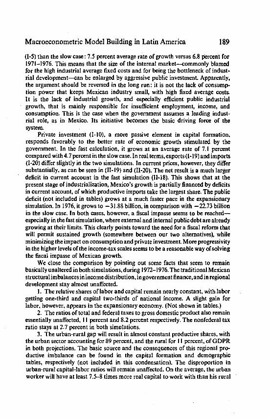
Macroeconometric Model Building in Latin America 189
(1-5) than the slow case: 7.5 percent average rate of growth versus 6.8 percent for1971—1976. This means that the size of the internal market—commonly blamedfor the high industrial average fixed costs and for being the bottleneck of indust-rial development—can be enlarged by aggressive public investment. Apparently,the argument should be reversed in the long run: it is not the lack of consump-lion power that keeps Mexican industry small, with high fixed average costs.It is the lack of industrial growth, and especially efficient public industrialgrowth, that is mainly responsible for insufficient employment, income, andconsumption. This is the case when the government assumes a leading indust-rial role, as in Mexico. Its initiative becomes the basic driving force of thesystem.
Private investment (1-10), a more passive element in capital formation,responds favorably to the better rate of economic growth stimulated by thegovernment. In the fast calculation, it grows at an average rate of 7.1 percentcompared with 4.7 percent in the slow case. In real terms, exports (1-19) and imports(1-20) differ slightly in the two simulations. In current prices, however, they differsubstantially, as can be seen in (11-19) and (11-20). The net result is a much largerdeficit in current account in the fast simulation (11-18). This shows that at thepresent stage of industrialization, Mexico's growth is partially financed by deficitsin current account, of which productive imports take the largest share. The publicdeficit (not included in tables) grows at a much faster pace in the expansionarysimulation. In 1976, it grows to —31.88 billion, in comparison with —22.73 biLlionin the slow case. In both cases, however, a fiscal impasse seems to be reached—especially in the fast simulation, where external and internal public debt are alreadygrowing at their limits. This clearly points toward the need for a fiscal reform thatwill permit sustained growth (somewhere between our two alternatives), whileminimizing the impact on consumption and private investment. More progressivityin the higher levels of the income-tax scales seems to be a reasonable way of solvingthe fiscal impasse of Mexican growth.
We close the comparison by pointing out some facts that seem to remainbasically unaltered in both simulations, during 1972—1976. The traditional Mexicanstructural imbalances in income distribution, in government finance, and in regionaldevelopment stay almost unaffected.
1. The relative shares of labor and capital remain nearly constant, with laborgetting one-third and capital two-thirds of national income. A slight gain forlabor, however, appears in the expansionary economy. (Not shown in tables.)
2. The ratios of total and federal taxes to gross domestic product also remainessentially unaffected, 11 percent and 8.2 percent respectively. The nonfederal taxratio stays at 2.7 percent in both simulations.
3. The urban-rural gap will result in almost constant productive shares, withthe urban sector accounting for 89 percent, and the rural for 11 percent, of GDPRin both projections. The basic source and the consequences of this regional pro-ductive imbalance can be found in the capital formation and demographictables, respectively (not included in this condensation). The disproportion inurban-rural capital-labor ratios will remain unaffected. On the average, the urbanworker will have at least 7.5—8 times more real capital to work with than his rural

190 Economic and Social Research in Latin America
counterpart in both cases.'5 The effects of the continuation of the productive gapwill be to maintain a steady migratory flow to the urban centers (Mexico City,Guadalajara, Monterrey and towns bordering on the United States), with theconsequent pressures on city facilities, enlargement of the "belts of poverty" aroundmetropolitan areas, and growth of urban unemployment and underemployment.16
A Final Word
In closing, we would like, to formulate briefly our stand on some importantquestions commonly asked with regard to econometric models as empirical toolsfor the analysis of growth in the LDC's.
Specification of developing-country models poses a challenge in building anew macro theory, but why go to the next step and create formal statistical models?Since we are in the economic-model business, we have thought often about thisquestion and have formulated answers to the frequent charges that LDC data arepoor in quality and sparsely available, and that economic behavior is erratic orirrational.
Economists are masters at working with poor and inadequate data. The issuefor econometricians is to make as much systematic sense as possible Out of sparse,"noisy" data. The basic statistical materials for the deyeloping countries are, inmany respects, like those we had to work with twenty or thirty years ago in theindustrial countries. Our MDC models now stand on firmer footing as a result ofall the spadework of the intervening years.
Economic and social problems are so intractable that we should do every-thing possible to make gains in knowledge, no matter how modest. It is for modest,systematic gains that we are working with macromodels of LDC's. The mostsophisticated methods must be applied to eke out precious gains. Much of thesophistication concerns the attempt to obtain estimates of parameters that areconsistent in the statistical sense of the term. This is extremely important becausethe most useful application of macromodels of the LDC economies is in simulationsof long-term growth patterns. In such studies, biases (lack of consistency) build upover time and can throw decade growth results far off track.
Methods of dealing in modern econometrics with "undersized" samples havebeen developed, and it is with these methods in mind that we have tackled theempirical task of implementing this measurement of the econometric structure ofMexico. We hope that it can set a pattern for future econometric research in therest of Latin America.
The actual capital-labor ratios result in 15 to 16 times more capital per worker in the urbanthan in the rural sector for 1972—76. We have halved them in order to account for the lack of data onprivate rural capital.
'61t should be remembered that even the fast calculation does not reduce the present unemploy-ment and underemployment rates—whatever they are in 1971. The only thing it does is to keep themconstant over the period.