NBER WORKING PAPER SERIES

MACROECONOMIC MISERY BY LEVELS OF INCOME IN AMERICA

Martin Ravallion

Working Paper 29050http://www.nber.org/papers/w29050

NATIONAL BUREAU OF ECONOMIC RESEARCH1050 Massachusetts Avenue

Cambridge, MA 02138July 2021

The author thanks George Eckerd, Toshihiko Mukoyama and Dominique van de Walle for helpful comments on an earlier draft. The views expressed herein are those of the author and do not necessarily reflect the views of the National Bureau of Economic Research.

NBER working papers are circulated for discussion and comment purposes. They have not been peer-reviewed or been subject to the review by the NBER Board of Directors that accompanies official NBER publications.

© 2021 by Martin Ravallion. All rights reserved. Short sections of text, not to exceed two paragraphs, may be quoted without explicit permission provided that full credit, including © notice, is given to the source.

Macroeconomic Misery by Levels of Income in AmericaMartin RavallionNBER Working Paper No. 29050July 2021JEL No. D31,E31,E32

ABSTRACT

Thirty years of distributional data are used to study the short-term impacts of popular macroeconomic indicators on real household incomes from the poorest to the richest Americans. The appropriate weights on unemployment versus inflation vary across the distribution. The unemployment rate matters at all levels, but especially so for the poorest. Inflation rates matter at middle incomes, though Okun’s famous Misery Index only performs well for the top income groups. GDP growth matters at all levels and proportionately more for the poorest, though only via the unemployment rate. Recessions are poverty-increasing, and skewness-decreasing, but with ambiguous effects on overall inequality.

Martin RavallionDepartment of EconomicsGeorgetown UniversityICC 580Washington, DC 20057and NBERmr1185@georgetown.edu

A data appendix is available at http://www.nber.org/data-appendix/w29050

2

1. Introduction

The relative importance of unemployment versus inflation as macroeconomic indicators

has long been debated. Arthur Okun’s famous “Misery Index” (OMI hereafter) weighted the two

indicators equally.2 While there are continuing concerns about the threat posed by high inflation,

the consensus today would appear to be on the side of those who have long contended that

unemployment should have higher weight than in the OMI.3

The main question addressed by this paper is how the relative importance of these two

macro indicators depends on whether one is talking about the real incomes of the poor, middle-

income groups or the rich.

Economic theory has offered some insights. Consider inflation. Market frictions can

entail that wages and other income sources are unlikely to be fully indexed and so short-term real

effects of inflationary shocks are likely. This could well differ by income. Recent “HANK”

models—new Keynesian models with heterogeneous agents—have pointed to the possibility of

systematic differences in what poor versus rich people would consider ideal monetary policy

responses to the threats posed by inflation.4 Differences in the extent of dependence on the labor

market, alongside the existence of frictions in that market, can readily generate differences in the

impacts of anti-inflation measures. The rich could well be in a better position than others to

protect their real incomes from inflation, through their access to multiple non-monetary assets,

thus maintaining a relatively high rate of return to their wealth.5 By contrast, poor people tend to

hold a higher share of their wealth as money balances, and so are impacted more by inflation.6

The importance of this wealth effect to poor people is a moot point, however, given that they

have little wealth, and what wealth they have often yields a low return.

There is evidence that higher inflation rates have been poverty increasing in developing

countries, though often with higher inflation rates than the U.S.7 The relevance of these findings

to the U.S. over the last 30 years is unclear. Inflation rates in the U.S. have been relatively low—

2 Okun introduced the Misery Index while he served as an advisor to the Johnson Administration during the 1960s. 3 See, for example, Blank and Blinder (1986), Di Tella et al. (2001) and Blanchflower et al. (2014). 4 An example is found in Gornemann et al. (2016). On the implications for specific monetary policies see Feiveson et al. (2020). 5 See Paola, and Camera (2009). This is consistent with the evidence that the rich in America obtain a higher rate of return to their wealth, which is one factor generating inequality (Cao and Luo 2017). 6 See, for example, the analysis in Erosa and Ventura (2002). 7 The literature is reviewed in Ravallion (2016a, Part 3). Using cross-country data, Easterly and Fischer (2001) found that poor people are more likely than the rich to identify inflation as a national policy concern.

3

comfortably under 5% per annum—since the early 1990s. Even so, the concern about inflation

remains, and with a distributional dimension. Since around 2019, the U.S. Federal Reserve has

been interested in understanding the distributional consequences of monetary policy and has

explicitly included promoting “broad-based and inclusive outcomes” as a policy goal (Board of

Governors 2020). At the time of writing (mid-2021), there is a public debate in the U.S.

stemming from fears that the macro policies in the wake of the 2020-21 pandemic are

stimulating inflation. Concerns have been raised about the impacts of macro policy choices on

poverty and inequality.8

Turning to unemployment, this too can be expected to matter differently at different

levels of income. Theoretical support for this view is found in the model-based simulations done

by Krusell et al. (2009). These indicate a “U” shape in the welfare gains from eliminating

business cycles, with larger gains for the poorest and the richest strata, though for different

reasons. In the Krusell et al. model, the impact on the poorest is a welfare effect given that they

are the more adversely impacted by risk, while the richest gain from higher interest rates, as

induced by the lower aggregate (precautionary) savings with smoothed business cycles.

We can also postulate that the poorest will incur the largest proportionate impact on their

incomes from a rise in the overall unemployment rate under the (plausible) assumption that they

depend most on relatively unskilled and more casual labor, which is hit hardest by a recession, as

demonstrated by Mukoyama and Şahin (2006). The middle-income group is still vulnerable to

being laid off in a down-turn, but less so than the poor. This is a minor concern for the rich, on

the other hand; for them, it is the impact of a recession on their wealth and its rate of return that

are the key concerns (as in the Krusell and Smith 1999).

The theoretical arguments suggest potentially complex distributional effects. Losses at all

levels imply first-order dominance, with unambiguously higher poverty measures.9 Greater

proportionate losses in both tails of the distribution, relative to the middle, suggest a more

complex impact on relative distribution, including measures of inequality.

If valid, these issues have important implications for social policy responses to the

business cycle, possibly pointing to the need to strengthen antipoverty policies when the

unemployment rate rises. However, the political economy of social policy may well work against

8 See, for example the discussion in the Economist (2020). 9 This holds for a broad class of additive poverty measures (Atkinson 1987).

4

that outcome. These macro indicators have political salience, including a potential influence on

electoral outcomes.10 If the more politically influential income groups are affected differently by

these macro indicators then other groups may be exposed to unfavorable macroeconomic

policies, with implications for how the distribution of income evolves. This may interact with the

political economy of redistributive policy, to the extent that the business cycle influences the

propensity of middle-income groups to support such policies. Lupu and Pontusson (2011)

modify the classic median-voter model to introduce “social affinity” whereby the income-

distance from the median to the poor, relative to that from the median to the rich, matters to the

degree of support the median voter will give to redistribution. To the extent that the business

cycle alters this aspect of income distribution it may also spillover to influence social policy

more broadly.

While such theoretical arguments can provide useful insights, we need empirical

evidence, which can also help calibrate and assess the models. Micro evidence can tell us (for

example) whether poorer families have higher rates of unemployment. However, macro evidence

can also reveal indirect effects on real incomes; for example, a higher economy-wide

unemployment rate may reduce the wage-bargaining power of workers in poor families or reduce

(public or private) transfer payments to those families. There is also likely to be heterogeneity

within any given income group, such as due to differences in dependence on the labor market,

wage setting, discrimination by race or gender, and wealth portfolios. It is thus of interest to see

if systematic differences in the mean impacts of these macro variables are evident at different

levels of income.

In an important paper in the literature on poverty in America, Blank and Blinder (1986)

found a strong business-cycle effect on the poverty rate, identified through a regression on the

unemployment rate using data over 1959-83. They concluded that “Despite many denunciations

of inflation as ‘the cruelest tax,’ there is little doubt that unemployment, not inflation, actually

bears most heavily on the poor.” (Blank and Blinder, 1986, p.9). The subsequent literature in the

1980s and ‘90s has been broadly consistent with this view; see, for example, Cutler and Katz

(1991) and Blinder et al. (1993). There has been an overlapping empirical literature on the

10 See, for example, the results of Adrangi and Macri (2019) on the influence of the OMI on the popularity of U.S. Presidents.

5

effects of macro variables on measures of inequality, including Blinder and Esaki (1978), Mocan

(1999) and Barlevy and Tsiddon (2006).

The paper explores these issues using real income distributions assembled from almost 30

years of survey data since the 1980s, spanning a wide range of macro-outcomes, including the

Great Recession (GR) of 2009-10. The overview of the literature above suggests that no single

summary measure of “inequality” could adequately capture the nature of the distributional

changes. The issues raised concern the effects of the classic macro variables on the levels of real

income, so this is what will be studied here rather than income shares or inequality (although

comments will be made about implications for inequality, including the Gini index). Impacts will

be studied across multiple quantiles of the distribution. Heathcote et al. (2010) calculated

multiple quantiles in describing the evolution of the distribution of income in the U.S.; they

found signs that recessions hurt the poor (echoing the earlier literature) but did not test the

impacts of the main macro indicators. Also a finer lens is needed at the lower end than provided

by Heathcote et al., reflecting the concerns about how the “poorest” are doing, which is often

seen as a parameter of social progress.11 Here one must recognize that there is a potentially

spurious variability in incomes at the bottom end, due to transient factors and measurement

errors. Some averaging is called for. The paper draws on the measure of the “floor” to the

distribution proposed by Ravallion (2016b) and estimated for the U.S. by Jolliffe et al. (2019).

In specifying the macroeconomic “misery” indicators, it has also been argued that the

OMI should be augmented to include the growth rate of GDP (negatively weighted).12 So, the

test regressions will include this covariate as well as the two indicators proposed by Okun. In the

regression specifications, emphasis will be given to testing for short-term impacts of the

macroeconomic indicators.

The paper’s results indicate a systematic pattern in how the key macroeconomic

indicators influence real incomes in America. The unemployment rate should have higher weight

than inflation in a Misery Index calibrated to real incomes across the whole distribution, at least

in this time period. A higher unemployment rate unambiguously increases poverty measures (for

all measures and lines). It also reduces the skewness of the distribution—an effect that is not

11 This is often identified with the Rawlsian principles of justice (Rawls 1971), although Rawls recognized the need for some averaging of incomes among the lowest stratum. For further discussion see Ravallion (2016a,b). 12 See, for example, the discussions in Barro (1999) and Hanke (2021).

6

evident in its (ambiguous) implications for inequality. Inflation matters more in the middle of the

distribution than in the tails. GDP growth rates matter at all levels of income, and especially for

the poorest; however, this effect is largely attributable to the impact of growth on the

unemployment rate. The restrictions implied by the OMI—namely equal weighs on

unemployment and inflation and excluding the GDP growth rate—are rejected across the bulk of

the distribution, and strongly so for the poorer strata; indeed, the OMI appears to only be

defensible for the top income groups.

After describing the data and measures used, Section 3 presents the main results, while

Section 4 discusses various extensions and tests. Section 5 concludes.

2. Data and measures

The distribution of household real income per person will be represented by points on the

quantile function, 𝑦𝑦(𝑝𝑝), which is the inverse of the cumulative distribution function, 𝑝𝑝 = 𝐹𝐹(𝑦𝑦),

giving the proportion 𝑝𝑝 of the population with an income below 𝑦𝑦. For example, one such point

is the median, namely 𝑦𝑦(0.50). An even spread of points across the domain of the quantile

function is adequate across the bulk of the distribution, but more detail is needed in the tails. For

top incomes, a narrower spacing is used, up to 𝑦𝑦(0.99).

The lower tail calls for another measure. For example, the series for 𝑦𝑦(0.01)

(analogously to 𝑦𝑦(0.99)) is not very informative. (The 𝑦𝑦(0.01) series has high variance in the

early period and mostly zero or close to it after the mid-1990s.) Some sort of averaging is clearly

called for when we focus on the lower end of the distribution. In addition to looking at 𝑦𝑦(0.10)

and 𝑦𝑦(0.20), the following analysis will study impacts on estimates of the “floor,” defined as a

weighted mean income of those in the poorest quintile, with higher weights on lower incomes

(following Ravallion 2016b).13 The weights are assumed to follow a power function with a

parameter 𝛼𝛼; for 𝛼𝛼 = 1 the weights decline linearly as income rises until one reaches 𝑦𝑦(0.20)

while for 𝛼𝛼 = 2 the weights decline as a quadratic function of income, giving a steeper increase

in the higher weight attached to poorer people in estimating the floor. The measures are referred

13 An option is to use the official poverty line instead of 𝑦𝑦(0.20). However, short-run changes in the inflation rate can then have spurious effects on the measured level of the floor, given that the inflation rate is also used to adjust the official poverty line.

7

to as 𝐹𝐹𝐹𝐹𝐹𝐹𝐹𝐹𝐹𝐹(𝛼𝛼) (𝛼𝛼 =1,2). Since this is a new measure, the Appendix provides a fuller

explanation.

These measures are calculated from the micro data for 29 rounds of the Annual Social

and Economic Supplement to the Current Population Survey, giving a series spanning 1988 to

2016.14 The measure of “income” is interpretable as market income. The components are money

income before taxes from several sources (such as wages, salary, net-income from self-

employment, social security payments, pensions, interest, dividends, alimony, other forms of

periodic monetary income). The income aggregate excludes capital gains and non-cash benefits

such as fringe benefits or noncash social assistance programs.15

Figure 1(a) plots the logs of the floor and selected quantiles. The rise in inequality is

evident, with a trend increase in top income quantiles, alongside a trend decline in the floor. For

example, in 2010 prices, the estimated level of the floor in 2016 is $5.50 per person per day (for

𝛼𝛼 = 2) while it was $7.18 in 1988.

Figure 1(b) provides a closer look at the bottom of the distribution, giving 𝑦𝑦(0.20) as

well as the two measures of the floor, and the poverty rate based on the official poverty lines. As

one would expect, there is co-movement among these measures. For example, in the GR period

we see a sharp rise in the poverty rate alongside a sinking floor. But it is not a perfect

correspondence. For example, in the mid-1990s, the declining poverty rate came alongside a

drop in the floor for 𝛼𝛼 = 2 and the drop in the poverty rate toward the end of the GR was not

initially matched by a rise in the floor.

The macroeconomic indicators are from standard sources. GDP is from U.S. National

Accounts, using the series for GDP per capita in constant prices as published in the World

Bank’s World Development Indicators. The monthly unemployment rates are those published by

the Federal Reserve, while the inflation rate is based on the Consumer Price Index (CPI) as

produced by the U.S. Bureau of Labor Statistics. With relative price changes and non-homothetic

preferences, one reason that inflation rates based on the CPI may predict poorly at the tails is that

the weights may only be valid nearer the middle. However, the CPI is the most widely used (by

far) macro indicator for inflation, so that is what is used here. The highest monthly

14 The calculations were done for Jolliffe et al. (2019), which discusses the methods and caveats. 15 Thus, it is essentially the same measure of family income is used as in the US official poverty measures. See Jolliffe et al. (2019) for further discussion.

8

unemployment rate in each year was used; this slightly outperformed both the mean

unemployment rate and the mid-year rate in specification tests using regressions for the log

median income. Figure 2 gives the macro indicators.

A striking feature of the data is the negative correlation between the level of the floor and

the economy-wide unemployment rate. The floor falls by about $0.30 a day for each 1% point

rise in the unemployment rate. The regression coefficients are -0.34 (s.e.=0.05) and -0.29 (0.06)

with correlation coefficients of -0.77 and -0.64 for 𝛼𝛼 = 1 and 𝛼𝛼 = 2 respectively. (The

Addendum provides graphs of the relationship.) We will see in the next section if this holds up

when we allow for the dynamics of the floor over time, and other macro indicators. Since the

focus here is on the short-term co-movements with the macroeconomic variables, all the

regressions are dynamic (including the lagged dependent variable) and they include a time trend.

The current-year values of the macro variables are used. (Section 4 notes some implications of

lagging the unemployment rate.)

The regressions do not control for the GR. As is obvious from Figure 2, this saw a

dramatic rise in the unemployment rate—5% points between March 2008 and March 2010. This

as an important clue to the distributional effects of macro shocks, and so it would not make sense

to control for it in the regressions.

3. Main results

For the logs of each level of household income, Table 1 provides regressions on the three

macro indicators—the unemployment rate and the inflation rate and the growth rate of GDP per

capita.

Looking first at the unemployment rate, we see that it has a strong (negative) effect at all

income levels. Comparing regression coefficients horizontally in Table 1, a marked “U” shape is

evident, with the largest (more negative) effect at the floor, but the next largest for the top 1%.

(Of course, the rich may face little direct threat to their own employment from a higher

economy-wide unemployment rate, but still be vulnerable to the associated business-cycle

effects, including through their wealth and the returns to that wealth.)

The difference in semi-elasticities across the distribution is notable. For the floor and top

1% we are looking at a semi-elasticity for the unemployment rate around -2.4 (even higher for

the floor with 𝛼𝛼 = 2), while it is about half that around the middle of the distribution. Consider,

9

for example, a 5% point increase in the aggregate unemployment rate (as we saw in the GR). We

would expect to see a 6% decline in real household incomes around the middle of the

distribution, but around 12% at the bottom and top.

Finding that a higher unemployment rate reduces all levels of income implies an

unambiguous increase in poverty over all poverty lines and measures.16 (Section 4 discusses the

quantitative implications for the official poverty measures in the U.S., but this finding does not

depend on the precise poverty line used.)

The implications for relative distribution are more comples. By comparing the

coefficients for the floor and each quantile in Table 1 with that for the mean in Table 2 (Columns

1 and 2), we can see that a higher unemployment rate shifts relative incomes (“mean-

normalized”) down at the bottom and top, but shifts them up around the middle. (This also holds

if one makes “median-normalized” comparisons.) Table 1 also gives the long-run semi-

elasticities for the unemployment rate. The “U” shape is somewhat muted but still present; the

highest value is at 𝑦𝑦(0.10) (twice the value at 𝑦𝑦(0.70)), while the next highest is 𝑦𝑦(0.99).

This combination of reduced inequality above the median and higher inequality below it

will clearly reduce the overall (positive) skewness in the distribution. To quantify this effect in a

summary statistic, let us define:17

𝑆𝑆𝑆𝑆𝑆𝑆𝑆𝑆(𝛼𝛼) ≡𝑦𝑦(0.99)/𝑦𝑦(0.50)

𝑦𝑦(0.50)/𝐹𝐹𝐹𝐹𝐹𝐹𝐹𝐹𝐹𝐹(𝛼𝛼)

Intuitively, one can think of this as the “tails ratio:” the ratio of the upper tail’s spread of incomes

to that of the lower tail. Using the same regression specification as in Table 1 one obtains the

regression for 𝑆𝑆𝑆𝑆𝑆𝑆𝑆𝑆(2) reported in Table 2.18 As can be seen in Column (4), the unemployment

rate has a negative effect on 𝑆𝑆𝑆𝑆𝑆𝑆𝑆𝑆 (significant at the 2% level). The long run effect of the

unemployment rate is -5.075 (s.e.=1.533), which is significant at the 1% level.

It can be noted that this effect of unemployment on the skewness measure above is not

evident in another (popular) indicator of skewness, namely the ratio of the mean to the median

(Table 2, Columns 5 and 6). The impact of unemployment is greater for the mean than for the

16 This holds within a broad class of additive measures, as shown in Atkinson (1987). (Note that first-order dominance of quantile functions implies the same for CDFs.) 17 This is similar to a measure used by Lupu and Pontusson (2011), and we give the measure the same name, “SKEW;” the main difference is that Lupu and Pontusson use the top and bottom 10%. This is a natural measure in this context. 18 The following results are qualitatively similar using 𝛼𝛼 = 1.

10

median (Table 1), but the difference is not statistically significant. The mean-median ratio (or

difference) is clearly too crude a measure to pick up the effect.

The skewness effect we see in the data with regard to the relative-income effects of a

higher unemployment rate is clearly going to be ambiguous with regard to its impact on overall

inequality.19 One can think of this pattern as combining two opposing redistributions of income

associated with higher unemployment, namely a regressive shift below the median, and

progressive one above the median. The outcomes for overall inequality will depend on the

precise measure of inequality used. (The next section will consider one popular measure.)

This also suggests a relationship between the structure of inequality and the business

cycle with implications for redistributive policy. Applying the argument of Lupu and Pontusson

(2011), the present results suggest that redistributive effort may decline in recessions, since they

stretch the gap between the poorest and the median, while compressing that between the richest

and the middle. Conversely, support for redistribution increases in macroeconomic expansions.

Thus, the (well-known) tendency for governmental macro intervention to increase in recessions,

as a means of macro stabilization, may well come with attenuated effort at redistribution.

Turning to the inflation rate, we find that this is statistically significant for the bulk of the

distribution, but not at the tails (Table 1). The regression coefficient on inflation is small and

insignificant for the floor. The coefficient stays high for the top incomes, but the standard error is

high. This is suggestive of a high variance in the ability of the rich to protect their real incomes

from inflation—some do better than others in this regard. Notice also that the inflation rate has

no significant effect on SKEW (in the regression above). This is because the proportionate effect

of inflation on top incomes is not significantly different to its effect on the median income.

There is no significant effect of a higher inflation rate on 𝑆𝑆𝑆𝑆𝑆𝑆𝑆𝑆 (Table 2).

As seen in Table 1, there is generally no significant short-term effect of the GDP growth

rate. (The one exception is for 𝑙𝑙𝑙𝑙𝑙𝑙𝑦𝑦(0.20).) The next section examines this more closely.

Separately to these short-term (contemporaneous) effects, we see underlying longer term

trends entailing a small but statistically significant decline in the level of the floor but positive

trends for all quantiles, and with a steeper positive trend as one goes up the distribution, peaking

at the top (Table 1). This is picking up the trend increase in inequality in America.

19 Skewness is not, of course, the same thing as inequality. A perfectly symmetric density function of incomes can have large inequality but it has zero skewness by definition.

11

Returning to Okun’s Misery Index, Table 1 also gives the tests of the parameter

restrictions implied by the OMI, namely that the index attaches equal weight to the inflation and

unemployment rates, and it does not include GDP growth independently. These restrictions only

pass for the upper end of the distribution, and are convincingly rejected for the lower half, for

which the OMI over-weights the inflation rate. The source of the general failure of the OMI is

that it under-weights unemployment rather than excluding the growth rate.

4. Further tests20

While the Phillips Curve has clearly been rather flattened in this period in the U.S., to the

extent that the curve remains at work, the inflation rate will be a decreasing function of the

unemployment rate. Without identifying and testing for a Phillips Curve we can simply re-

estimate the regressions in Table 1 as reduced form relationships, dropping the inflation rate.

This makes very little difference to the results. The coefficients on the unemployment rate

change little, and still exhibit the U-shape. This is consistent with expectations based on a greatly

flattened Phillips Curve.

The role of the GDP growth rate as a macro variable is of obvious interest. It might be

surprising that the GDP growth rate matters so little in the results of Table 1. However, these are

partial effects. if one drops the other two macro indicators, one finds a strong positive effect of

higher GDP growth rates on 𝑆𝑆𝑆𝑆𝑆𝑆𝑆𝑆 (Table 2). This is also true for both measures of the floor

and all quantiles (Addendum).21 (For the overall mean of household income, the elasticity is

about 0.9; see Table 2, Column 1.) The floor is highly responsive to growth, with an elasticity of

1.6 or more, but this falls as one reaches middle income levels. The elasticity is about 0.8 by

𝑦𝑦(0.70), but then picks up as one reaches the richest 1%.22 The growth effect is largely

attributable to fluctuations in the unemployment rate. Only adding unemployment greatly

attenuates the coefficient on GDP growth. Not also that if one lags the unemployment rate by

20 This section only summarizes results. Further details are found in the Addendum. 21 The coefficient on the lagged dependent variable rises with this change (relative to Table 1), and it is not significantly different from unity. So, once one drops the unemployment rate and inflation rate, the regressions are essentially growth rates of household income regressed on the growth rate of GDP per capita. Specification tests confirmed this; on regressing the log median on its own lagged value, the current and lagged log GDP per capita, one could not reject the null that the coefficient on the former is unity and the sum of the coefficients on the two GDP variables is unity (F=0.76, prob.=0.48). 22 This is consistent with the stylized fact reported by Guvenen et al. (2017) for US log earnings data when regressed on GDP growth.

12

one year, the GDP growth rate becomes significant at all income levels (Addendum). GDP

growth is clearly picking up the current unemployment rate.

The calculations of the floor include non-positive incomes in the CPS. An unemployment

shock could push some families to zero income. Of course, this is a real effect. Nonetheless, one

might ask if the effect of the unemployment rate on the floor in Table 1 is mainly due to these

income collapses. The estimated population share of such incomes is 1.4% on average, varying

from 0.6% to 2.2% and this is correlated with the unemployment rate (r=0.42). Adding a control

for the share of non-positives does not, however, eliminate the unemployment effect on the floor,

though its coefficient falls in absolute value, to -1.770 (HAC s.e.=0.519) and -1.894 (0.580) for

and for 𝛼𝛼 =1, 2 respectively.

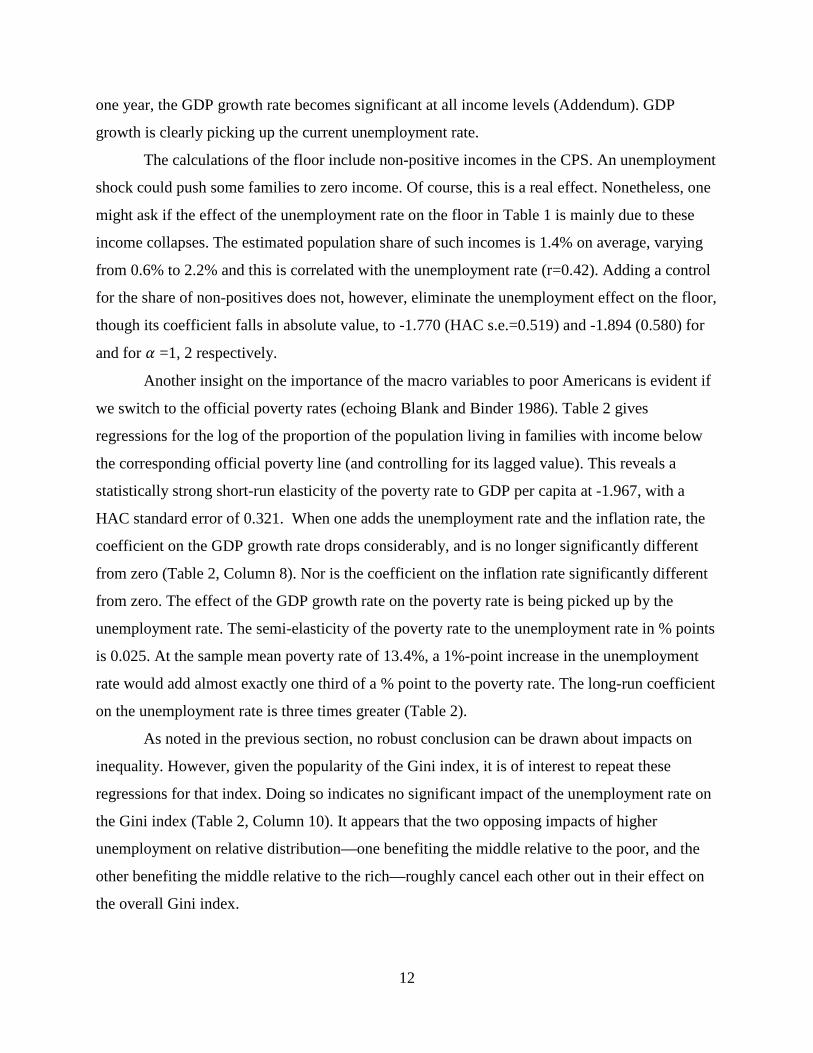
Another insight on the importance of the macro variables to poor Americans is evident if

we switch to the official poverty rates (echoing Blank and Binder 1986). Table 2 gives

regressions for the log of the proportion of the population living in families with income below

the corresponding official poverty line (and controlling for its lagged value). This reveals a

statistically strong short-run elasticity of the poverty rate to GDP per capita at -1.967, with a

HAC standard error of 0.321. When one adds the unemployment rate and the inflation rate, the

coefficient on the GDP growth rate drops considerably, and is no longer significantly different

from zero (Table 2, Column 8). Nor is the coefficient on the inflation rate significantly different

from zero. The effect of the GDP growth rate on the poverty rate is being picked up by the

unemployment rate. The semi-elasticity of the poverty rate to the unemployment rate in % points

is 0.025. At the sample mean poverty rate of 13.4%, a 1%-point increase in the unemployment

rate would add almost exactly one third of a % point to the poverty rate. The long-run coefficient

on the unemployment rate is three times greater (Table 2).

As noted in the previous section, no robust conclusion can be drawn about impacts on

inequality. However, given the popularity of the Gini index, it is of interest to repeat these

regressions for that index. Doing so indicates no significant impact of the unemployment rate on

the Gini index (Table 2, Column 10). It appears that the two opposing impacts of higher

unemployment on relative distribution—one benefiting the middle relative to the poor, and the

other benefiting the middle relative to the rich—roughly cancel each other out in their effect on

the overall Gini index.

13

5. Conclusions

When assessed by predictive power for changes in the real incomes of Americans since

the late-1980s, a macroeconomic Misery Index should put higher weight on unemployment than

on inflation, and especially so for the poorest. For both the poorest and the richest Americans,

the variance seen in the inflation rate over this period has little or no short-term explanatory

power for real incomes. For the poorest, the effect of inflation is swamped by the unemployment

rate, consistent with earlier findings in the literature for the period from the 1950s through to the

mid-1980s. For the richest 1% it is more likely that their real incomes can be protected well

against moderate inflation rates. The short-term impact of differences in the GDP growth rate on

household incomes is largely accountable to changes in the current unemployment rate.

The appropriate weights in the Misery Index look very different for the bulk of the

middle of the distribution as compared to the tails. The proportionate impacts on real household

incomes of a higher macro unemployment rate are greatest for the poorest and richest

Americans. The semi-elasticities fall to about half their peak values toward the middle of the

distribution. From the 20th percentile through to the middle and upper-middle segments of the

distribution, we also see significant effects of differences in the inflation rate, which is almost

(but never exactly) as important as the unemployment rate around the upper-middle.

Statistically, one can reject Okun’s famous misery index for all except the high-income

strata. Okun’s index fails most dramatically for the poorest. However, an important caveat is that

this was a period of relatively low inflation in the U.S. While not so low as to prevent

identification of its real income effects for much of the distribution, one should not conclude that

substantially higher inflation rates would continue to be of secondary importance to

unemployment, including for poor Americans.

These findings imply an unambiguous increase (decrease) in poverty (for any poverty

line and measure) associated with higher (lower) unemployment rates. The implications for

relative distribution during the business cycle are more complex. Recessions tend to hurt all

levels of income absolutely, but less so for the middle strata than the tails. In other words, the

pattern in the data suggests that recessions tend to be skewness-reducing, i.e., inequality

increasing for the bottom half, and inequality decreasing among the top half. This more complex

pattern is not evident if one only looks at a summary statistic of overall inequality, such as the

popular Gini index.

14

The political-economy implications of these findings depend heavily on how political

power is mapped into the income distribution. This is not the place to take a position on that

issue, but one can note the possible difference in implications. If it is the middle and upper-

middle strata that have the greatest political influence then macro policies will tend to attach

greater importance to controlling inflation than would be in the interest of either tail of the

distribution, and especially the poorest.

This might well change if those in the richest stratum exercise the greatest political

power, although that is less clear from this paper’s results. Granted, inflation is not a statistically

significant predictor of the real incomes of the richest stratum, but this could well reflect

divergent effects within the stratum (noting that the point estimate is still high for the effect of

inflation; it is the standard error that blows up at the very top).

Nor should the paper’s finding that the unemployment rate is a strong predictor of the

real incomes of the rich be taken to imply that the rich would support any policies to reduce the

unemployment rate. The statistical significance could well reflect correlated aspects of the

business cycle rather than direct impacts of reducing the unemployment rate. This merits further

investigation.

15

Appendix: Formula for the floor

Observed (survey-based) household incomes are denoted 𝑦𝑦𝑖𝑖 (i=1,…, n), in a population

of size n. There is uncertainty as to whether 𝑦𝑦𝑚𝑚𝑖𝑖𝑚𝑚 = 𝑚𝑚𝑚𝑚𝑚𝑚(𝑦𝑦𝑖𝑖, 𝑚𝑚 = 1, . . . ,𝑚𝑚) is in fact the floor,

given measurement errors and transient effects. Following Ravallion (2016b) it is postulated that

any observed income level within an agreed poor stratum has some (non-zero) probability of

being the true floor. The ordinary (equally-weighted) mean income of incomes in this stratum is

not a plauible measure as not all incomes in this group are equally likely to emerge as the lowest

level of living if one could remove the transient effects and errors. The relevant probabilities are

not, of course, data, and assumptions are required. It is assumed that the probability of being the

poorest household declines as the observed measure of income rises. More precisely, one

postulates a corresponding (unobserved) distribution 𝑦𝑦𝑖𝑖∗, after eliminating the ignorable transient

effects and measurement errors. The floor of the 𝑦𝑦𝑖𝑖∗ distribution is 𝑦𝑦𝑚𝑚𝑖𝑖𝑚𝑚∗ = min (𝑦𝑦𝑖𝑖∗, 𝑚𝑚 = 1, …𝑚𝑚).

𝑦𝑦𝑚𝑚𝑖𝑖𝑚𝑚∗ as a random variable, with a probability distribution given the data such that the estimate of

𝑦𝑦𝑚𝑚𝑖𝑖𝑚𝑚∗ is ∑ 𝜙𝜙𝛼𝛼(𝑦𝑦𝑖𝑖)𝑦𝑦𝑖𝑖𝑚𝑚𝑖𝑖=1 where 𝜙𝜙𝛼𝛼(𝑦𝑦𝑖𝑖) = 𝑃𝑃𝑃𝑃𝑙𝑙𝑃𝑃(𝑦𝑦𝑖𝑖 = 𝑦𝑦𝑚𝑚𝑖𝑖𝑚𝑚∗ ) is the probability that person i, with 𝑦𝑦𝑖𝑖,

is the worst off person in the 𝑦𝑦∗ distribution. Following Ravallion (2016b), the calculations in

this paper assume the following functional form satisfying these assumptions:

𝜙𝜙𝛼𝛼(𝑦𝑦𝑖𝑖) = 𝐼𝐼𝑖𝑖�1−

𝑦𝑦𝑖𝑖𝑧𝑧 �

𝛼𝛼

∑ �1−𝑦𝑦𝑗𝑗𝑧𝑧 �

𝛼𝛼𝑦𝑦𝑗𝑗≤𝑧𝑧

for 𝛼𝛼 > 0 (1)

Here 𝐼𝐼𝑖𝑖 = 1 if 𝑦𝑦𝑖𝑖 ≤ 𝑧𝑧 and 𝐼𝐼𝑖𝑖 = 0 otherwise. For 𝛼𝛼 > 0, 𝜙𝜙𝛼𝛼(𝑦𝑦𝑖𝑖) attains its maximum value for

𝑦𝑦𝑚𝑚𝑖𝑖𝑚𝑚 = min (𝑦𝑦𝑖𝑖 , 𝑚𝑚 = 1, …𝑚𝑚) and then falls monotonically with 𝑦𝑦𝑖𝑖, until it reaches zero at some

value z, above which there is no chance of someone with that income being the poorest. Under

this assumption, Ravallion (2016b) shows that:

𝐹𝐹𝐹𝐹𝐹𝐹𝐹𝐹𝐹𝐹(𝛼𝛼) = 𝑆𝑆(𝑦𝑦𝑚𝑚𝑖𝑖𝑚𝑚∗ �𝑦𝑦𝑚𝑚, 𝑚𝑚 = 1, …𝑚𝑚;𝛼𝛼) = 𝑧𝑧(1 − 𝑃𝑃𝛼𝛼+1/𝑃𝑃𝛼𝛼) (2)

Here, 𝑃𝑃𝛼𝛼 is the Foster-Greer-Thorbecke (FGT) (1984) class of poverty measures, as defined by

𝑃𝑃𝛼𝛼 ≡1𝑚𝑚∑ (1 − 𝑦𝑦𝑖𝑖

𝑧𝑧)𝛼𝛼𝑦𝑦𝑖𝑖≤𝑧𝑧 . However, the parameter 𝛼𝛼 has a different interpretation to that in the

FGT index since in this context 𝛼𝛼 is the curvature parameter for the probability function used for

weights in estimating the floor, instead of being an ethical inequality-aversion parameter as in

FGT.

16

References

Adrangi, Bahram, and Joseph Macri, 2019, “Does the Misery Index Influence a U.S. President’s

Political Re-Election Prospects?” Journal of Risk and Financial Management 12(1): 1-

11.

Atkinson, Anthony B., 1987, “On the Measurement of Poverty,” Econometrica 55: 749-764.

Barlevy, Gadi, and Daniel Tsiddon, 2006, “Earnings Inequality and the Business Cycle,”

European Economic Review 50(1): 55-89.

Barro, Robert, 1999, “Reagan Vs. Clinton: Who's The Economic Champ?” Bloomberg.

Blanchflower, David .G., David Bell, Alberto Montagnoli, and Mirko Moro, 2014, “The

Happiness Trade-Off between Unemployment and Inflation,” Journal of Money, Credit

and Banking 46: 117-141.

Blank, Rebecca M., and Alan Blinder, 1986, “Macroeconomics, Income Distribution and

Poverty,” In Fighting Poverty: What Works and What Doesn't, edited by Sheldon H.

Danziger and Daniel H. Weinberg. Cambridge, Mass.: Harvard University Press.

Blank, Rebecca M., David Card, Frank Levy and James L. Medof, 1993, “Poverty, Income

Distribution, and Growth: Are They Still Connected?” Brookings Papers on Economic

Activity 1993(2): 285-339.

Blinder, Alan S. and Howard Y. Esaki, 1978, “Macroeconomic Activity and Income Distribution

in the Postwar United States,” Review of Economics and Statistics 60(4): 604-609.

Board of Governors, 2020, “Guide to Changes in the 2020 Statement on Longer-Run Goals and

Monetary Policy Strategy,” Board of Governors, U.S. Federal Reserve.

Boel, Paola, and Gabriela Camera, 2009, “Financial Sophistication and the Distribution of the

Welfare Cost of Inflation,” Journal of Monetary Economics 56)7): 968-978.

Cao, Dan, and Wenlan Luo, 2017, “Persistent Heterogeneous Returns and Top End Wealth

Inequality,” Review of Economic Dynamics 26: 301–326.

Cutler, David, and Lawrence Katz, 1991, “Macroeconomic Performance and the

Disadvantaged,” Brookings Papers on Economic Activity 1991(2): 1-74.

Di Tella, Rafael, Robert J. MacCulloch and Andrew J. Oswald, 2001, “Preferences over Inflation

and Unemployment: Evidence from Surveys of Happiness,” American Economic Review

91(1): 335- 341.

17

Easterly, William and Stanley Fischer, 2001, “Inflation and the Poor,” Journal of Money, Credit

and Banking 33(2): 160-178.

Economist, The, 2020, “Starting Over Again: The Covid-19 Pandemic is Forcing a Rethink in

Macroeconomics,” The Economist July 25.

Erosa, Andres, and Gustavo Ventura, 2002, “On Inflation as a Regressive Consumption Tax,”

Journal of Monetary Economics 49(4): 761-795.

Feiveson, Laura, Nils Goernemann, Julie Hotchkiss, Karel Mertens and Jae Sim, 2020,

“Distributional Considerations for Monetary Policy Strategy,” Finance and Economics

Discussion Series, 2020-073, Divisions of Research & Statistics and Monetary Affairs

Federal Reserve Board, Washington, D.C.

Ferreira, Francisco, and Martin Ravallion, 2009, “Poverty and Inequality: The Global Context,”

in The Oxford Handbook of Economic Inequality, edited by Wiemer Salverda, Brian

Nolan and Tim Smeeding, Oxford: Oxford University Press.

Foster, James, J. Greer, and Erik Thorbecke, 1984, “A Class of Decomposable Poverty

Measures,” Econometrica 52: 761-765.

Gornemann, Nils, Keith Kuester and Makoto Nakajima, 2016, “Doves for the Rich, Hawks for

the Poor? Distributional Consequences of Systematic Monetary Policy,” International

Finance Discussion Papers 1167, Board of Governors of the Federal Reserve System.

Guvenen, Fatih, Sam Schulhofer-Wohl, Jae Song, and Motohiro Yogo, 2017, “Worker Betas:

Five Facts about Systematic Earnings Risk,” American Economic Review Papers and

Proceedings 107(5): 398–403.

Hanke, Steve, 2021, “Hanke’s 2020 Misery Index: Who’s Miserable and Who’s Happy?,”

National Review (Online), April 14.

Heathcote Jonathan, Fabrizio Perri and Giovanni Violante, 2010, “Unequal We Stand: An

Empirical Analysis of Economic Inequality in the US, 1967-2006,” Review of Economic

Dynamics 13: 15-51.

Jolliffe, Dean, Juan Margitic and Martin Ravallion, 2019, “Food Stamps and America’s

Poorest,” NBER Working Paper 2605.

Krusell, Per, Toshihiko Mukoyama, Ayşegül Şahin, and Anthony A. Smith, 2009, “Revisiting

the Welfare Effects of Eliminating Business Cycles,” Review of Economic Dynamics 12:

393–404.

18

Krusell, Per, and Anthony Smith, 1999. “On the Welfare Effects of Eliminating Business

Cycles,” Review of Economic Dynamics 2: 245–272.

Lupu, Noam and Jonas Pontusson. 2011. “The Structure of Inequality and the Politics of

Redistribution,” American Political Science Review 105(2): 316‐336.

Mocan, Naci, 1999, “Structural Unemployment, Cyclical Unemployment, and Income

Inequality,” Review of Economics and Statistics 81(1): 122-134.

Mukoyama, Toshihiko, and Ayşegül Şahin, 2006, “Costs of Business Cycles for Unskilled

Workers,” Journal of Monetary Economics 53: 2179-2193.

Newey, Whitney and Kenneth West, 1987, “A Simple Positive Semi-Definite, Heteroskedasticity

and Autocorrelation Consistent Covariance Matrix,” Econometrica 55: 703–708.

Paul, Mark, William Darity Jr., and Darrick Hamilton, 2017, “Why we Need a Federal Job

Guarantee,” Jacobin.

Ravallion, Martin, 2016a, Economics of Poverty: History, Measurement and Policy. New York:

Oxford University Press.

______________, 2016b, “Are the World’s Poorest Being Left Behind?” Journal of Economic

Growth 21(2): 139–164.

Rawls, John, 1971, A Theory of Justice. Cambridge Mass.: Harvard University Press.

19

Figure 1: Incomes across the distribution

(a) Whole distribution

1

2

3

4

5

6

1988 1992 1996 2000 2004 2008 2012 2016

Log

hous

ehol

d in

com

e pe

r per

son

($ p

er d

ay)

y(0.99)

y(0.90)

y(0.50)

y(0.20)

Floor(1)Floor(2)

(b) Closer look at the lower tail

05

1015202530

10 11 12 13 14 15 16

1988 1992 1996 2000 2004 2008 2012 2016

Poverty rate (right axis)

20th quantile (q(0.2; left axis)

Floor (alpha=1; left axis)

Floor (alpha=2; left axis)

Inco

me

($20

10 p

er d

ay)

Poverty rate

(% below

official line)

20

Figure 2: Macroeconomic indicators

-4

-2

0

2

4

6

8

10

12

1988 1992 1996 2000 2004 2008 2012 2016

Unemployment rateInflation rateGDP p.c. growth rate

Mac

roec

onom

ic in

dica

tor (

% p

er a

nnum

)

Table 1: Regressions for the levels of household income on three macro variables

𝐹𝐹𝐹𝐹𝐹𝐹𝐹𝐹𝐹𝐹(𝛼𝛼) 𝑦𝑦(𝑝𝑝) 𝛼𝛼 = 2 𝛼𝛼 = 1 𝑝𝑝 = 0.10 𝑝𝑝 = 0.20 𝑝𝑝 = 0.50 𝑝𝑝 = 0.70 𝑝𝑝 = 0.90

𝑝𝑝 = 0.95

𝑝𝑝 = 0.99

Constant 13.586***

(2.697) 5.709*** (1.403)

-1.143 (1.320)

-1.025 (0.593)

-2.513*** (0.483)

-3.042*** (0.668)

-4.576*** (1.011)

-5.995*** (1.502)

-9.905** (3.582)

Lagged dep. var. 0.380*** (0.084)

0.498*** (0.066)

0.683*** (0.050)

0.671*** (0.035)

0.683*** (0.060)

0.709*** (0.058)

0.666*** (0.071)

0.636*** (0.079)

0.615*** (0.111)

Unemployment rate -3.064*** (0.381)

-2.482*** (0.266)

-2.225*** (0.379)

-1.545*** (0.136)

-1.180*** (0.148)

-1.022*** (0.110)

-1.254*** (0.305)

-1.910*** (0.427)

-2.341** (0.932)

Inflation rate -0.068 (0.391)

-0.294 (0.284)

-0.563 (0.500)

-0.742*** (0.308)

-0.815*** (0.106)

-0.925*** (0.200)

-1.001*** (0.159)

-1.111*** (0.247)

-1.027 (0.931)

Growth rate of real GDP per capita

-0.464 (0.405)

-0.089 (0.270)

0.170 (0.215)

0.198** (0.094)

0.126 (0.131)

0.210** (0.083)

0.134 (0.162)

-0.119 (0.257)

-0.033 (0.506)

Year -0.006*** (0.001)

-0.002*** (0.001)

0.001 (0.001)

0.001*** (0.000)

0.002*** (0.000)

0.002*** (0.000)

0.003*** (0.001)

0.004*** (0.001)

0.006*** (0.002)

R2 0.966 0.950 0.911 0.939 0.982 0.987 0.980 0.971 0.926 Long-run coeff. for unemployment rate

-4.941*** (0.444)

-4.941*** (0.531)

-7.009*** (1.588)

-4.688*** (0.571)

-3.724*** (0.414)

-3.511*** (0.519)

-3.750*** (0.705)

-5.246*** (0.844)

-6.073*** (1.710)

Test of OMI: F stat. (prob.)

18.711 (0.000)

27.160 (0.000)

8.396 (0.002)

10.884 (0.001)

7.462 (0.003)

3.605 (0.044)

1.563 (0.232)

1.958 (0.165)

1.785 (0.191)

Note: n=28; HAC standard errors in parentheses are robust to the presence of both heteroskedasticity and autocorrelation of unknown form (assuming that the autocorrelations fade out for more distant observations); see Newey and West (1987). ***: 1% significance; **: 5%; *10%. Growth rate is ∆𝑙𝑙𝑚𝑚𝑙𝑙𝑙𝑙𝑃𝑃. Inflation rate is ∆𝑙𝑙𝑚𝑚𝑙𝑙𝑃𝑃𝐼𝐼. Unemployment rate is fraction of the workforce. Note that, to provide more accuracy, the variables are scaled as fractions (rather than % points). (Regression coefficients should be divided by 100 to obtain the coefficients for % point values.)

22

Table 2: Regressions for summary statistics of the distribution of income

Log mean household income per person

Log 𝑆𝑆𝑆𝑆𝑆𝑆𝑆𝑆(2) Log (mean/median) Log poverty rate (F(𝑧𝑧))

Log Gini index

(1) (2) (3) (4) (5) (6) (7) (8) (9) (10) Constant -2.710*

(1.397) -4.592***

(0.880) 3.964

(3.558) 3.950

(4.422) -1.471** (0.589)

-1.728* (0.883)

2.254 (1.659)

2.076** (0.978)

-2.881** (1.132)

-2.799 (1.848)

Lagged dep. var.

0.873*** (0.076)

0.668*** (0.065)

0.724*** (0.078)

0.570*** (0.112)

0.739*** (0.088)

0.700*** (0.110)

0.919*** (0.066)

0.672*** (0.049)

0.744*** (0.107)

0.713*** (0.145)

Unemployment rate

-1.368*** (0.310)

-2.184** (0.876)

-0.144 (0.202)

2.466*** (0.273)

-0.090 (0.217)

Inflation rate -0.868*** (0.203)

0.994 (1.051)

-0.057 (0.209)

0.024 (0.378)

-0.326 (0.230)

Growth rate of real GDP p.c.

0.876*** (0.127)

0.099 (0.169)

1.129*** (0.291)

0.046 (0.448)

0.058 (0.119)

-0.009 (0.136)

-1.967*** (0.321)

-0.436 (0.285)

-0.053 (0.104)

-0.094 (0.132)

Year 0.002* (0.001)

0.003*** (0.001)

-0.002 (0.002)

-0.002 (0.002)

0.001** (0.000)

0.001** (0.000)

-0.001 (0.001)

-0.001*** (0.000)

0.001** (0.001)

0.001 (0.001)

Long-run coeff. for unemp. rate

-4.122*** (0.079)

-5.075*** (1.533)

7.513 (1.289)

R2 0.948 0.981 0.728 0.783 0.869 0.872 0.867 0.943 0.932 0.935 Note: n=28; HAC standard errors in parentheses (see Table 1 notes). ***: 1% significance; **: 5%. Growth rate is ∆𝑙𝑙𝑚𝑚𝑙𝑙𝑙𝑙𝑃𝑃. Inflation rate is ∆𝑙𝑙𝑚𝑚𝑙𝑙𝑃𝑃𝐼𝐼. Unemployment rate is fraction of the workforce.