Embed Size (px)
Citation preview

MACROECONOMIC INTERACTIONS BETWEEN LATIN AMERICA AND CHINA-INDIA IN A DYNAMIC
INTERTEMPORAL MODEL OF THE WORLD ECONOMY
Rodrigo Suescún♣
The World Bank
Abstract This paper develops a perfect foresight dynamic intertemporal general equilibrium model of the world economy to study the nature of the short-run adjustment process and the likely quantitative impact of economic, trade policy and financial reform developments in China and India on the Latin America region as a whole. A sequence of simulation experiments suggests that tariff reductions, rapid growth and financial liberalization reform in China and India have minor negative effects on GDP and technological growth, consumption and investment in Latin America and relatively stronger effects - but still small - on trade patterns, financial capital inflows, FDI and relative prices. Trade liberalization and rapid economic growth based on productivity growth in China and India likely depress relative prices of primary commodities and manufactures produced in the developing world, causing a slight deterioration of the Latin America region’s terms of trade. However, the trade balance to GDP ratio improves slightly over the medium term as exports increase while imports fall somewhat. The destinations for Latin America exports tilt away from China and India and toward developed country markets as its exports become cheaper in those markets while imports from the developed world are substituted, in relative terms, with cheaper imports from China and India. Foreign direct investment flows toward Latin America fall by less than 1% relative to trend. With the emergence of China-India as a marginal net creditor to the rest of the world, FDI inflows in the future may come from this region, competing with developed countries for the role of FDI source. JEL Classification: F17, F41, F43
♣ The author wishes to thank Dominique Van Der Mensbrugghe for his helpful comments on an earlier version and María Fernanda Rosales for excellent research assistance. All errors remain responsibility of the author. The views expressed in this paper are those of the author and should not be interpreted as reflecting those of the World Bank.

1. Introduction
The rapid growth and increasing integration into the international trade and financial
systems of the two largest Asian economies, China and India, have been a major source
of concern both in developed and developing countries during the last decade and a half.
Much of the public debate and economic discussion on the global-, regional- or country-
level implications of these developments has been cast in terms of a rather descriptive
and partial contrast between challenges and opportunities. Up to now, this casting has
paid little attention to their likely impact on Latin America and, more importantly, little
attention has paid to provide quantitative assessments. It is high time to address the issue
from quantitative and Latin American perspectives.
This paper develops a dynamic intertemporal general equilibrium model of the world
economy for analyzing the effect of China’s and India’s economic, trade policy and
financial reform developments on the Latin America region, with a focus on the linkages
among trade, foreign direct investment (FDI), financial capital flows and productivity
growth. In contrast to standard static trade models, our dynamic approach provides a
unified framework for understanding not only long-run effects on resource allocations,
relative prices, trade direction, and growth but also for understanding the dynamic path of
adjustment, the focus of much public debate. The short-run implications for
unemployment, wage inequality, balance of payments, FDI diversion, sectoral
adjustment, etc. of Asian developments may not be fully understood by policymakers in
the region or may be perceived as costly. The understanding of the short-run economic
adjustment is critical for avoiding counterproductive policy responses in the region.
The paper is structured as follows. Section 2 provides a brief description of the main
features of the world economy model. Section 3 presents the formal theoretical model.
Section 4 includes a brief discussion of the solution algorithm. Section 5 describes the
baseline calibration process and Section 6 sets up the sequence of numerical experiments
and presents and discusses simulation results. Finally, Section 7 concludes.
2
2. Overview of the Model
Consider a world consisting of three regions indexed by {1,2,3}j = and inhabited by
households each. World household population is constant and normalized to unity, i.e.
. Region 1 corresponds to the developed world part and is composed of
the major industrial economies (including Korea, Hong Kong-China and Singapore);
Region 2 comprises China and India (and also the rest of Asia) and Region 3 represents
Latin America and the Caribbean. The three regions are both intratemporally and
intertemporally linked by flows of trade in differentiated products - allowing for
incomplete specialization in production and trade - and by flows of differentiated real
assets - financial capital and foreign direct investment (FDI). Regions 2 and 3 share
exactly the same underlying economic structure, differing only in how the economies are
calibrated to match regional averages. Their major difference with Region 1 is based on
the empirical fact that OECD countries are the primary source of FDI.
jN
1=N∑ j{1,2,3}∈j
1 Consequently,
Region 1 is the only net supplier of FDI and Regions 2 and 3 are modeled as competing
net FDI importers.2
Another important difference lies in the nature of the growth process. Region 1 is
modeled as the technological leader whose rate of technical progress is given by the rate
at which the world technology frontier improves and is assumed constant for simplicity.
Regions 2 and 3 lag behind the frontier of knowledge and benefit from a process of
diffusion of innovations created in Region 1, since knowledge is considered non-rival.
However, in contrast to a pure public good, knowledge is partially excludable and FDI is
deemed as the main vehicle through which technology and knowledge transfers occur.
Accordingly, the growth rate is determined endogenously and depends on the gap
between the level of technology embodied in the stock of foreign capital in place and the
1 According to the JBIC Institute (2002) OECD countries accounted for over 90% of global outward FDI in 1998-2000. 2 Empirical support to this modeling choice is also given by the JBIC Institute (2002): China and Latin America were the major recipients of FDI in 1998-2000, attracting 85% of total FDI flows outside the OECD area.
3

region’s own level of technical efficiency. Region 1 investors fail to internalize the effect
of their investment decisions abroad on productivity growth in recipient countries.
It must be noted that along the transitional path the growth rate can be accelerated by FDI
inflows but along the steady-state equilibrium growth path, due to the process of
technological catch up, the growth rate will be dictated by the rate of technical progress
in the developed world. The idea of technology transfers through FDI has been explored
by Glass and Saggi (1998) who provide a theoretical rationale for the limited ability of
developing countries to attract state-of-the-art technologies through FDI. The FDI-growth
nexus has been the subject of a large body of empirical literature. After appraising 16
empirical studies, the JBIC Institute (2002, p. 31) claims that the “(…) vast majority of
the studies reviewed (…) indicate that FDI does make a positive contribution to both
income growth and factor productivity in host countries.”3 The literature has also shown
that the link between FDI and growth depends on the characteristics of the recipient
country (degree of openness, human capital, trade regime, political and economic
institutions, etc.). In the present model, the absorptive capacity and social capabilities of
the host regions are taken as given.
Each region produces two types of internationally traded goods indexed by .
Because goods with the same name but produced in different regions are regarded by
consumers and producers as different goods, as imperfect substitutes, they need to be
distinguished by the pair , i.e., by industry and by place of production. Thus,
consistent with trade data, the model accounts for cross-hauling: simultaneous exports
and imports of goods of the same product category. Good
j H}{L,i =
i)(j,
{L}i = is a low-tech or
primary good which is produced with domestically owned capital and unskilled labor and
is used in all regions as intermediate input in the production of good . H
Good is a high-tech or manufacturing good which is produced with
domestically-owned capital, foreign-owned capital, skilled and unskilled labor and
{H}i =
3 For other and more critical assessments, see for instance Niar-Reichert and Weinhold (2001) and Nunnenkamp (2004).
4

intermediate inputs. Foreign ownership of productive assets introduces a wedge between
GDP and GNP statistics since part of the GDP will be owed to foreign investors. In
Regions 2 and 3 the production function is assumed to exhibit foreign capital-skill
complementarity. The skill premium, defined as the relative price of skilled labor in
terms of unskilled labor, is determined endogenously in the rational expectations
equilibrium and depends positively on two forces: the ratio of unskilled to skilled
employment (relative quantity effect) and the ratio of foreign-owned capital to skilled
employment (foreign capital-skill complementarity effect). Imports and domestic
production of the high-tech good are combined via an Armington aggregator into a single
composite final good.
Each region is inhabited by three types of infinitely-lived households differing in
borrowing-saving opportunities and skills. households are savers or Ricardian
consumers and the rest are spenders or liquidity-constrained consumers, if we make use
of Mankiw’s (2000) behavioral taxonomy, or they could be renamed as stakeholders and
workers, respectively, if we draw on Danthine and Donaldson’s (1995) terminology.
Liquidity-constrained households, in turn, are disaggregated into two skill groups: skilled
and unskilled workers. An exogenous fraction of the labor force is skilled and the
rest is unskilled.
wj,N
sj,N
The Ricardian/Non-Ricardian dichotomy has been introduced in the literature to
overcome the failure of the Barro-Ramsey model (and the Diamond-Samuelson model) to
explain why consumption follows closely the evolution of current income and the fact
that many households have net worth near zero. High-wealth households save and
consume but do not work, smooth consumption over time by trading in physical and
financial assets and act in an optimizing, forward looking manner. They own all the low-
and high-tech firms and the final good firm and are entitled to claim any profits that may
result. Spenders or low-wealth households follow the rule of thumb of consuming their
disposable labor income every period and do not save or borrow, rendering consumption
smoothing unfeasible.
5

Furthermore, the two types of salaried workforce face different labor market structures.
Skilled labor is inelastically supplied to the manufacturing sector and the corresponding
wage is set in a perfectly competitive market. The market for unskilled labor is
characterized by a real wage rigidity that arises from a right-to-manage bargaining
process between firms and workers (Nickell and Andrews, 1983; Layard, Nickell and
Jackman, 1991). In a right-to-manage framework a union represents all unskilled workers
and the union and the firms bargain over wages but the level of employment, and thereby
the level of equilibrium unemployment, is unilaterally determined by the firms. It is
assumed that a fraction of the unskilled labor force is available for work in the low-
tech producing sector and the rest , with
uj,LN
uj,HN 1NN uj,
Huj,
L =+ , is available for work in the
high-tech sector.
This general equilibrium framework can be used to study a wide range of policy issues in
dynamic macroeconomics. This paper develops a model of the world economy for
understanding and analyzing the effect on short-run adjustment as well as on long-run
resource allocation in Latin America of China and India’s growth developments and
deeper integration into the international economic system. To model trade liberalization,
it is assumed that each region has a government that levies tariffs on commodity imports
and rebates collected revenues back to (high-wealth) households as lump-sum transfer
payments. At the world equilibrium, all prices and quantities are determined
endogenously such that firms, unions and households maximize and individual, regional
and world resource constraints are satisfied. Regional current account imbalances are
exactly offset by capital flows, reflecting the region’s change in the net international
investment position, and the equilibrium world interest rate is consistent with financial
assets in zero net supply worldwide.
3. Model Formulation
This section provides a detailed description of the world economy model. To avoid
overly cumbersome notation, various conventions are adopted throughout the paper.
First, although, in principle, model parameters vary across regions, their dependence on
6

the index , that denotes the particular region, is not written explicitly. This shortcut
should cause no confusion. Second, all variables are measured in regional per capita
terms (unless otherwise stated) and no population growth is allowed. Third, following
convention, region-wide, per capita aggregates are represented by capital letters while
variables under the household’s control are denoted by lower case letters. The exceptions
are relative prices and rental rates which are written in lower case. In equilibrium,
individual choices and the corresponding aggregate counterparts should be identical.
Further, time is discrete and indexed by
j
t , ∞= ,,2,1t K , and each period t in the model
is assumed to be one year. The numeraire good is the good produced in Region 1
whose price is fixed at 1, . All agents are assumed to be endowed with perfect
foresight over the future path of trade policies.
H
t∀
3.1 The Developing World: Regions 2 and 3 {2,3})(j =
3.1.1 Technical Progress
Let represent an index of labor-augmenting technological progress. Region 1 is the
technological leader and expands the world technology (knowledge) frontier at a constant
gross rate : . The technology of follower regions, Regions 2 and 3, is
determined by catch-up opportunities described by:
jtZ
1η 1t
111t ZηZ =+
zα-1j
1-tzαj
tjt )(Z)(F=Z {2,3}j =
for , , being a measure of the speed of diffusion. This specification implies
that the current level of technology results from combining the technology of the lead
region and that reached so far by followers. It is assumed that technology is ingrained in
the level of foreign capital in place, where is the stock of capital per inhabitant of
Region owned by Region 1 investors. Since
Zα 0>α>1 Z
jtF
j j1-t
jt
jt ZZ=η , an expression for the law of
motion of the gross rate of growth can be obtained:
7
j1tZ1
1tj
1t
1t
jt1
Zjt ηlog)α(1
ZFZF
logηlogαηlog −−−
−+⎟⎟⎠
⎞⎜⎜⎝
⎛⎟⎟⎠
⎞⎜⎜⎝
⎛+= (1) {2,3}j =
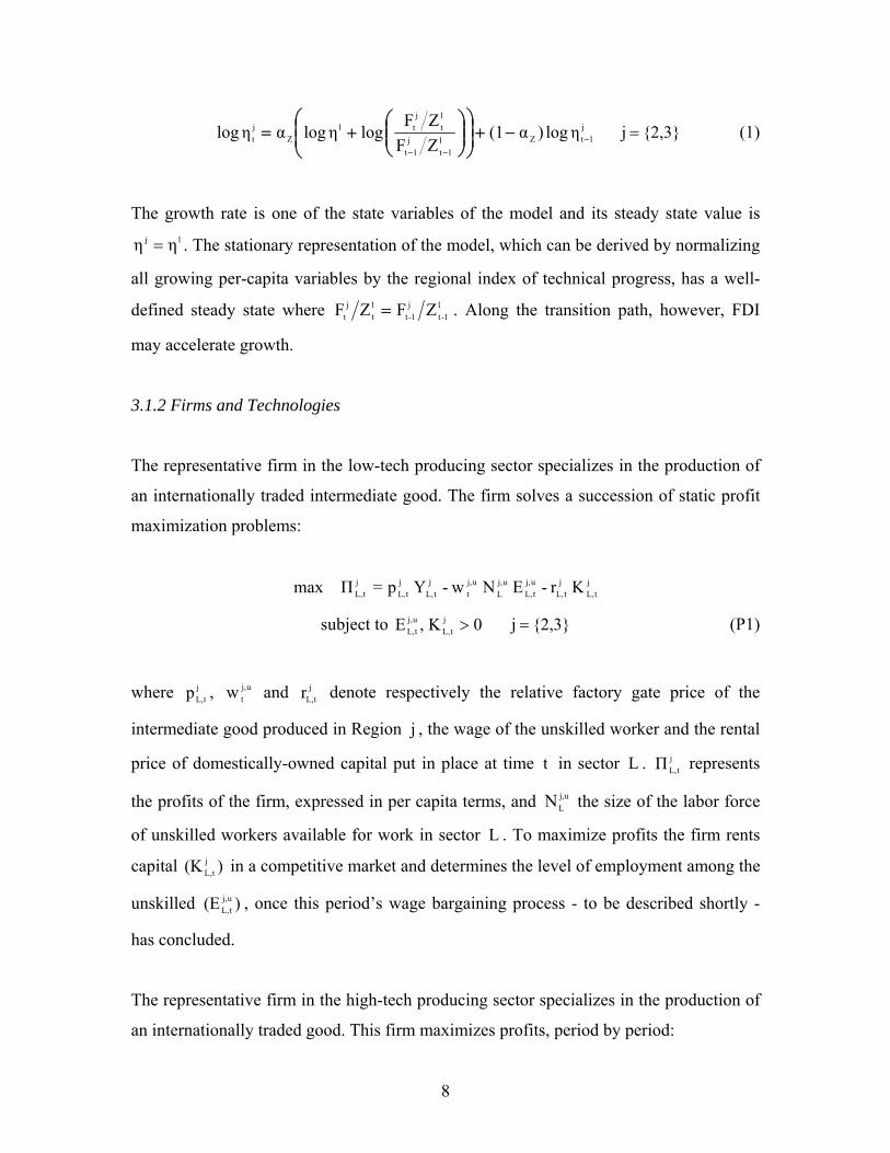
The growth rate is one of the state variables of the model and its steady state value is
. The stationary representation of the model, which can be derived by normalizing
all growing per-capita variables by the regional index of technical progress, has a well-
defined steady state where
1j ηη =
11-t
j1-t
1t
jt ZFZF = . Along the transition path, however, FDI
may accelerate growth.
3.1.2 Firms and Technologies
The representative firm in the low-tech producing sector specializes in the production of
an internationally traded intermediate good. The firm solves a succession of static profit
maximization problems:
j
tL,j
tL,uj,tL,
uj,L
uj,t
jtL,
jtL,
jtL, Kr-ENw-Yp=Πmax
subject to 0K,E jtL,
uj,tL, > {2,3}j = (P1)
where , and denote respectively the relative factory gate price of the
intermediate good produced in Region , the wage of the unskilled worker and the rental
price of domestically-owned capital put in place at time
jtL,p uj,
tw jtL,r
j
t in sector . represents
the profits of the firm, expressed in per capita terms, and the size of the labor force
of unskilled workers available for work in sector . To maximize profits the firm rents
capital in a competitive market and determines the level of employment among the
unskilled , once this period’s wage bargaining process - to be described shortly -
has concluded.
L jtL,Π
uj,LN
L
)(K jtL,
)(E uj,tL,
The representative firm in the high-tech producing sector specializes in the production of
an internationally traded good. This firm maximizes profits, period by period:
8

∑−+−−−−=∈{1,2,3}k
jk,tL,
jk,tL,
jt
jt
jtF,
jtH,
jtH,
sj,t
sj,sj,t
uj,tH,
uj,H
uj,t
jtH,
jtH,
jtH, YpF)ψ(rKrENwENwYpΠmax
subject to 0>Y,Y,Y,F,K,E,E j3,tL,
j2,tL,
j1,tL,
jt
jtH,
sj,t
uj,tH, {2,3}j = (P2)
where is the relative price of the manufacturing good produced in Region , and
denote the level of employment of unskilled and skilled workers in sector H ;
and denote the size of the labor force of unskilled and skilled workers available for
work in that sector and and are the corresponding wage rates measured in terms
of the numeraire. As mentioned before, unskilled wages and employment are determined
according to a right-to-manage bargaining process and skilled wages are determined in a
competitive market, and in equilibrium adjust so that demand and supply of skilled labor
match, i.e. , since the labor endowment is normalized to unity and supplied
inelastically. and denote the stock of capital owned by residents and by foreign
investors, both put in place for production in sector . and are the relative rental
prices of domestically- and foreign-owned capital and is an exogenously given risk
premium demanded by foreign investors for investment in Region .
jtH,p j uj,
tH,E
sj,tE uj,
HNs,jN
uj,tw sj,
tw
1E s,jt = t∀
jtH,K j
tF
H jtH,r j
tF,r
jtψ
j
jk,tL,Y is the amount of intermediate good per inhabitant of Region used in Region and
produced in Region , . is the relative price paid by the -sector firm
for the Region ’s intermediate input used in or imported by Region . Note that the
price of the intermediate good produced and sold domestically satisfies , while
the domestic price of imports is equal to the world price adjusted for tariffs, i.e.
, where represents bilateral tariff and non-tariff barriers applied to
imports from Region sold in Region .
j j
k {1,2,3}k ∈ jk,tL,p H
k jj
tL,jj,tL, pp =
ktL,
jk,tL,
jk,tL, p)τ(1p += jk,
tL,τ
k j
Both production technologies exhibit constant returns to scale. Value added in sector
is given by the following Cobb-Douglas production function:
L
)(Y jtL,
9

Lα-1uj,tL,
uj,L
jt
LαjtL,L
jtL, )EN(Z)(KAY = {2,3}j = (2)
for and for 0AL > 0α1 L >> j∀ . is a scaling factor and is the capital share.
Gross production in sector H is described by a two-level CES function. The top
level combines a valued added component and an intermediate good component
:
LA Lα
)(Y jtH,
)(VA jtH,
)(SjtH,
{ } Yσ1
YσjtH,Y
YσjtH,YH
jtH, )(S)ω(1)(VAωAY −+= {2,3}j = (3)
for , and 0ω1 Y ≥≥ 0AH > (0,1),0)(σY ∪−∞∈ for j∀ . is a parameter determining
the share of the two components,
Yω
Yσ is the substitution parameter determining the
elasticity of substitution between the value added and intermediate goods, given by
)σ(11 Y− , and is a shift parameter. HA
At the lower level of production, the value added component is described by a nested
CES technology:
( ) ( ) ( ){ } Vσ)Hα-(1
λσVσ
λσsj,t
sj,jtλ
λσjtλv
Vσuj,tH,
uj,H
jtV
HαjtH,v
jtH, ENZ)ω(1Fω)ω(1)EN(ZωKAVA ⎥
⎦
⎤⎢⎣
⎡−+−+=
{2,3}j = (4)
for , , 0ω,ω1 λV ≥≥ 0AV > (0,1),0)()σ,(σ λV ∪−∞∈ for j∀ . As before, these are
parameters of distribution, scale and substitution, respectively. (0,1)αH ∈ denotes the
share in output of capital owned by residents. The elasticity of substitution between
foreign capital and unskilled labor is )σ-(11 V and the elasticity of substitution between
foreign capital and skilled labor is )σ-(11 λ . Foreign capital-skill complementarity holds
when the elasticity of substitution between foreign capital and unskilled labor is higher
than that between foreign capital and skilled labor.
10

The equilibrium skill premium associated with this technology is given by:
vσ1
sj,
uj,tH,
uj,H
1λσVσ
λ
λσ
sj,
jt
λV
λVuj,
t
sj,t
NEN
)ω(1NF
ωω
)ω)(1ω(1ww
−−
⎟⎟⎠
⎞⎜⎜⎝
⎛
⎥⎥⎦
⎤
⎢⎢⎣
⎡−+⎟⎟
⎠
⎞⎜⎜⎝
⎛−−= (5) }3,2{j =
If , the production function exhibits foreign capital-skill complementarity, and
the skill premium increases with a rise in the stock of foreign capital relative to skilled
employment (foreign capital-skill complementarity effect) and increases with a rise in
unskilled employment relative to skilled employment (relative quantity effect) (see
Krusell et al., 2000).
λV σσ >
At the first level of production the other component is an aggregate intermediate input,
which is an Armington composite good:
( ) Sσ1
{1,2,3}k
Sσjk,tL,Sk,S
jtH, YωAS ⎟
⎠⎞⎜
⎝⎛ ∑=
∈ {2,3}j = (6)
for , , 0ω1 Sk, ≥≥ 0AS > (0,1),0)(σS ∪−∞∈ for j∀ . Without loss of generality the
’s are constrained to sum to one. The composite intermediate input is simply an
aggregate of intermediate goods produced in the three regions.
S,kω
Finally, the representative retailer firm in the final good sector uses type- goods, both
domestically produced and imported, as inputs to produce a composite final good. The
retailer firm solves the following problem:
H
∑−=∈{1,2,3}k
jk,tH,
jk,tH,
jtR,
jtR,
jtR, YpYpΠmax
subject to 0Y,Y,Y j3,tH,
j2,tH,
j1,tH, > {2,3}j = (P3)
11

where is the amount of good per inhabitant of Region used by Region
retailer and produced in Region k . is the relative price paid for the Region ’s good
used in or imported by Region . The price of good produced and sold
domestically satisfies: and
jk,tH,Y H j j
jk,tH,p k
H j Hj
tH,jj,tH, pp = 1pp 1
tH,1,1
tH, == , while the domestic price of imports
is equal to the corresponding world price adjusted for tariffs, i.e. ,
where represents bilateral tariff and non-tariff barriers applied to imports from
Region sold in Region . is an Armington aggregator:
ktH,
jk,tH,
jk,tH, p)τ(1p +=
jk,tH,τ
k j jtR,Y
( ) Rσ1
{1,2,3}k
Rσjk,tH,Rk,R
jtR, YωAY ⎟
⎠⎞⎜
⎝⎛ ∑=
∈ {2,3}j = (7)
where determines the Armington substitution elasticity and the ’s are Armington
aggregator weights. The final good is simply an aggregate of type- goods produced
worldwide.
Rσ Rk,ω
H
3.1.3 The Ricardian Household
In each region there are Ricardian households. This subsection specifies the
general problem faced by a representative saver/consumer. Note that in what follows all
variables are expressed not in per-capita terms over the whole population in the region
but in per-capita terms defined over the subset of high-wealth households. The
representative high-wealth household optimally chooses plans for consumption
, investment in physical capital in sector and investment in
physical capital in sector H to maximize its discounted lifetime utility:
j wj,N
)}({c 0twj,
t∞= L )}({i 0t
wj,tL,
∞=
)}({i 0twj,tH,
∞=
( )∑ −∞=0t
jt
jwj,t
t ZCclogβmax (8)
subject to
12

[ ] wj,t
wj,t
wj,tH,
jtH,
wj,tL,
jtL,
wj,tH,
wj,tL,
wj,t
jtR,
wj,tt
wj,1t TΠkrkriicpd)r(1d −−−−++++=+ (9)
wj,tL,
2
1wj,tL,
wj,tL,Lwj,
tL,wj,tL,
wj,1tL, kδ)1(η
ki
2ikδ)(1k ⎥
⎦
⎤⎢⎣
⎡+−−⎟
⎠⎞
⎜⎝⎛−+−=+
ϕ (10)
wj,tH,
2
1wj,tH,
wj,tH,Hwj,
tH,wj,tH,
wj,1tH, kδ)1(η
ki
2ikδ)(1k ⎥
⎦
⎤⎢⎣
⎡+−−⎟
⎠⎞
⎜⎝⎛−+−=+
ϕ (11)
givenk,k wj,H,0
wj,L,0 {2,3}j = (P4)
for and for 0δ),(β1 >> 0),( HL ≥ϕϕ j∀ . is the subjective discount factor, is the
depreciation rate, and are sectoral adjustment cost parameters, and
β δ
Lϕ Hϕ 0C j >
denotes the minimum level of stationary consumption per period in region .
denotes the stock of foreign debt, is the sum of profits earned by all firms and
claimed by high-wealth households and denotes all types of government transfers,
all expressed in terms of the numeraire good per high-wealth household. Equation (9) is
the household’s budget constraint and equations (10) and (11) are sectoral physical
capital accumulation laws with capital stocks subject to adjustment costs along the
transition path. The high-wealth household has access to a competitive world capital
market for non-contingent one-period real bonds where it can save and borrow at the
world interest rate , expressed in terms of the numeraire. Savings, investments and
financial capital flows are all the result of forward looking, intertemporal optimization
decisions.
j wj,td
wj,tΠ
wj,tT
tr
3.1.4 Skilled- and Unskilled-Wage Earners
There are skilled and unskilled workers and each of them is endowed with one
unit of time that is inelastically supplied. Skilled and unskilled wage earners do not
borrow or save and have only to decide how much to consume every period. The
representative skilled worker solves the following static maximization problem:
sj,N uj,N
13

( )jt
jsj,t ZCclogmax −
subject to sj,t
sj,t
jtR, wcp ≤
jt
sj,t ZCc ≥ {2,3}j = (P5)
On the other hand, some of the unskilled workers suitable for work in sector i ,
, are employed and some unemployed. Employed workers earn a net wage
and unemployed workers receive unemployment benefits , satisfying
and where is the gross wage replacement ratio.
Unemployment benefits are financed by taxes levied on unskilled wage income.
Formally, the unskilled worker solves the following problem:
H}{L,i =uj,
tuj, w)τ(1− uj,
tb
uj,t
uj,t
uj, bw)τ(1 >− uj,t
juj,t wζb = jζ
( )jt
juj,ti, ZCclogmax −
subject to
uj,
tuj,uj,
ti,j
tR, w)τ(1cp −≤ if employed
uj,t
uj,ti,
jtR, bcp ≤ if unemployed
jt
uj,ti, ZCc ≥ H}{L,i = {2,3}j = (P6 and P7)
The budget of the unemployment compensation system is balanced:
uj,
tuj,
tjuj,
tuj,
tuj,uj,
t )wE(1ζwEτT −−= (12)
where is the average employment rate among the unskilled workers,
, and is a government transfer.
uj,tE
uj,tH,
uj,H
uj,tL,
uj,L
uj,t ENENE += uj,
tT
14

3.1.5 Union Wage Bargaining
The interaction between firms and unskilled workers to determine wages and
employment is based on a version of the right-to-manage bargaining model in which a
union, that represents all unskilled workers, is assumed to exercise monopoly power to
determine wages so as to maximize the expected utility of its members and firms have the
right-to-manage power to determine how many workers to employ once wages have been
set.
The industry- union maximizes total expected utility which is a function of the utility
derived by a representative union member under alternative employment/unemployment
options. With probability the worker will be hired in sector and earn a net wage
and with probability
L
uj,tL,E L
uj,tL,
uj,L w)τ(1− )E(1 uj,
tL,− she will not be hired in that sector. Still in
this case she has outside options. With probability she can be hired in sector and
earn a net wage or with probability
uj,tH,E H
uj,tH,
uj,H w)τ(1− )E(1 uj,
tH,− she can remain unemployed
and receive unemployment benefits for . The union maximizes its objective function
with respect to subject to the constraint that wage-employment outcomes,
determined by unions and firms, are on the labor demand curve and taking as given the
alternative wage. Formally, the optimal wage solves the union’s problem:
uj,tH,b
uj,tL,w
⎥⎥⎥⎥⎥
⎦
⎤
⎢⎢⎢⎢⎢
⎣
⎡
⎪⎭
⎪⎬⎫
⎪⎩
⎪⎨⎧
⎟⎟⎠
⎞⎜⎜⎝
⎛−−+⎟
⎟⎠
⎞⎜⎜⎝
⎛−
−−
+⎟⎟⎠
⎞⎜⎜⎝
⎛−
−
jjt
uj,tH,
jtR,
uj,tH,
jjt
uj,tH,
jtR,
uj,Huj,
tH,uj,tL,
jjt
uj,tL,
jtR,
uj,Luj,
tL,
uj,L
CZb
p1log)E(1C
Zw
p)τ(1logE)E(1
CZ
wp
)τ(1logE
Nmax
subject to
15
⎟⎟⎠
⎞⎜⎜⎝
⎛⎟⎟⎠
⎞⎜⎜⎝
⎛
⎥⎥⎥⎥⎥
⎦
⎤
⎢⎢⎢⎢⎢
⎣
⎡
−=
uj,L
jt
jtL,
Lα1
jt
uj,tL,
jtL,
Luj,tL, N
1Z
K
Zw
p1
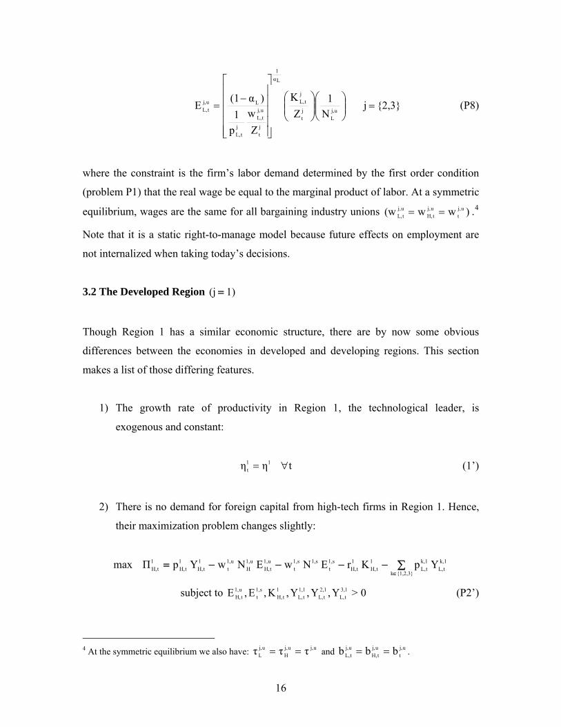
)α(1E {2,3}j = (P8)
where the constraint is the firm’s labor demand determined by the first order condition
(problem P1) that the real wage be equal to the marginal product of labor. At a symmetric
equilibrium, wages are the same for all bargaining industry unions .)ww(w uj,t
uj,tH,
uj,tL, == 4
Note that it is a static right-to-manage model because future effects on employment are
not internalized when taking today’s decisions.
3.2 The Developed Region 1)(j =
Though Region 1 has a similar economic structure, there are by now some obvious
differences between the economies in developed and developing regions. This section
makes a list of those differing features.
1) The growth rate of productivity in Region 1, the technological leader, is
exogenous and constant:
tηη 11t ∀= (1’)
2) There is no demand for foreign capital from high-tech firms in Region 1. Hence,
their maximization problem changes slightly:
∑−−−−=∈{1,2,3}k
k,1tL,
k,1tL,
1tH,
1tH,
s1,t
s1,s1,t
u1,tH,
u1,H
u1,t
1tH,
1tH,
1tH, YpKrENwENwYpΠmax
subject to (P2’) 0>Y,Y,Y,K,E,E 3,1tL,
2,1tL,
1,1tL,
1tH,
s1,t
u1,tH,
4 At the symmetric equilibrium we also have: uj,uj,
Huj,
L τττ == and uj,t
uj,tH,
uj,tL, bbb == .
16

3) Consequently, the production function does not display foreign capital-skill
complementarity:
( ) ( )[ ] Vσ)Hα-(1
Vσsj,t
sj,jtv
Vσu1,tH,
u1,H
1tV
Hα1tH,v
1tH, ENZ)ω(1)EN(ZωKAVA −+= (4’)
4) And the skill premium does not exhibit a foreign capital-skill complementarity
effect:
vσ1
s1,
u1,tH,
u1,H
V
Vu1,
t
s1,t
NEN
ω)ω(1
ww
−
⎟⎟⎠
⎞⎜⎜⎝
⎛−= (5’)
5) In contrast to other regions, the representative Ricardian household in Region 1
has to decide over FDI outflows and how to allocate them between Regions 2 and
3, since the developed world is modeled as the only net supplier of productivity-
enhancing FDI. Thus, the Ricardian household optimally chooses plans for FDI in
the two developing regions . The maximization intertemporal
program is now the following:
)}i,({i 0t3
tF,2
tF,∞=
( )∑ −∞=0t
1t
1w1,t
t ZCclogβmax (8’)
subject to
−−−⎥⎦
⎤⎢⎣
⎡⎟⎠
⎞⎜⎝
⎛+⎟
⎠
⎞⎜⎝
⎛+++++=+
w1,tH,
1tH,
w1,tL,
1tL,
3tF,w1,
32
tF,w1,
2w1,tH,
w1,tL,
w1,t
1tR,
w1,tt
w1,1t krkri
NNi
NNiicpd)r(1d
w1,t
w1,t
3t
3t
3tF,w1,
32t
2t
2tF,w1,
2w1,tH,
1tH, TΠF)ψ(R
NNF)ψ(R
NNkr −−+⎟
⎠
⎞⎜⎝
⎛−+⎟
⎠
⎞⎜⎝
⎛− (9’)
w1,tL,
2
1w1,tL,
w1,tL,Lw1,
tL,w1,tL,
w1,1tL, kδ)1(η
ki
2ikδ)(1k ⎥
⎦
⎤⎢⎣
⎡+−−⎟
⎠⎞
⎜⎝⎛ ϕ−+−=+ (10’)
17

w1,tH,
2
1w1,tH,
w1,tH,Hw1,
tH,w1,tH,
w1,1tH, kδ)1(η
ki
2ikδ)(1k ⎥
⎦
⎤⎢⎣
⎡+−−⎟
⎠⎞
⎜⎝⎛ ϕ−+−=+ (11’)
2t
2
12t
2tF,F22
tF,2t
21t Fδ)1(η
Fi
2iFδ)(1F ⎥
⎦
⎤⎢⎣
⎡+−−⎟
⎠⎞
⎜⎝⎛ ϕ−+−=+ (13)
3t
2
13t
3tF,F33
tF,3t
31t Fδ)1(η
Fi
2iFδ)(1F ⎥
⎦
⎤⎢⎣
⎡+−−⎟
⎠⎞
⎜⎝⎛ ϕ−+−=+ (14)
givenF,F,k,k 30
20
wj,H,0
wj,L,0 (P4’)
The stocks of capital built up abroad follow standard laws of motion. )F,(F 3t
2t
3.3 Resource Constraints
Prices and quantities are determined endogenously in the world equilibrium. At the world
equilibrium, relative prices must be set so that excess demand must be zero in every good
market, in all regions and at each time period. Equality of supply and demand in the
primary or low-tech good requires:
∑= ∈{1,2,3}kkj,tL,
kjtL,
j YNYN 3}2,{1,j = (15)
The equilibrium condition on the high-tech good market in all regions requires:
∑= ∈{1,2,3}kkj,tH,
kjtH,
j YNYN 3}2,{1,j = (16)
The market clearing condition in each period for the composite final good in all regions
is:
[ ] +++++= )ii(cNcNcY w1,tH,
w1,tL,
w1,t
w1,s1,t
s1,u1,t
1tR,
( ) ( ) (⎥⎥⎦
⎤
⎢⎢⎣
⎡∑
⎪⎭
⎪⎬⎫
⎪⎩
⎪⎨⎧
⎟⎟⎠
⎞⎜⎜⎝
⎛+−+⎟
⎠
⎞⎜⎝
⎛−+
∈
−
{2,3}k
k,1tH,
k,1tH,
k,1tL,
k,1tL,
k1,tH,
k1,tL,
1tL,1
kkt
kt
ktF,
k11tR, YpYpYYp
NNF)ψ(rN)(p ) (17a)
18

[ ] ++++++= − jtF,
j1jtR,
wj,tH,
wj,tL,
wj,t
wj,sj,t
sj,uj,t
jtR, iN)(p)ii(cNcNcY
( ) (⎥⎥⎦
⎤
⎢⎢⎣
⎡∑
⎭⎬⎫
⎩⎨⎧
+−+⎟⎠
⎞⎜⎝
⎛−+−
≠∈
−
jk{1,2,3}k
jk,tH,
jk,tH,
jk,tL,
jk,tL,
kj,tH,
jtH,
kj,tL,
jtL,j
kj
tjt
jtF,
j1jtR, YpYpYpYp
NNF)ψ(r)N(1)(p )
(17b) {2,3}j =
Equilibrium in the market for financial capital requires the condition that foreign assets
should be in zero net supply worldwide:
∑ ==∑ ∈∈ {1,2,3}jj
{1,2,3}jwj,
twj, 0DdN (18)
where denotes the region ’s total aggregate debt. As in Baxter and Crucini’s (1995)
approach, to compute the world’s general equilibrium one of the asset accumulation
equations has to be dropped since only two foreign debt stocks are independent. In fact,
equation (9’), the developed region asset accumulation equation, is dropped.
jD j
Finally, the government budget constraint is satisfied in each period in each region:
( )∑ +=≠
∈jk
{1,2,3}k
jk,tH,
ktH,
jk,tH,
jk,tL,
ktL,
jk,tL,
jt YpτYpτT 3}2,{1,j = (19)
The government’s role is to levy import tariffs and rebate revenues back to households in
a lump sum fashion.
4. Stationary Representation and Solution Method
As the knowledge frontier expands over time macroeconomic (per-capita) aggregates will
grow without bound and the world economy will become arbitrarily large. For
computational purposes it is convenient to work with the stationary representation which
can be derived by normalizing all growing per-capita variables by the corresponding
19
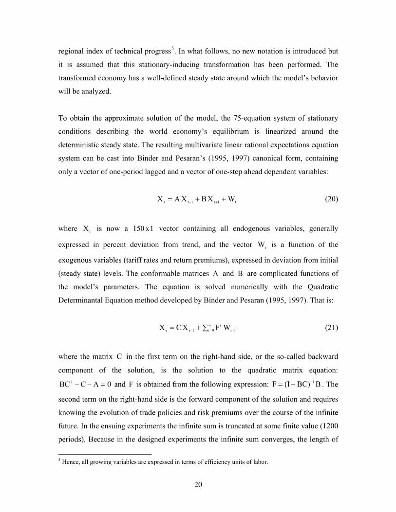
regional index of technical progress5. In what follows, no new notation is introduced but
it is assumed that this stationary-inducing transformation has been performed. The
transformed economy has a well-defined steady state around which the model’s behavior
will be analyzed.
To obtain the approximate solution of the model, the 75-equation system of stationary
conditions describing the world economy’s equilibrium is linearized around the
deterministic steady state. The resulting multivariate linear rational expectations equation
system can be cast into Binder and Pesaran’s (1995, 1997) canonical form, containing
only a vector of one-period lagged and a vector of one-step ahead dependent variables:
t1t1tt WXBXAX ++= +− (20)
where is now a vector containing all endogenous variables, generally
expressed in percent deviation from trend, and the vector is a function of the
exogenous variables (tariff rates and return premiums), expressed in deviation from initial
(steady state) levels. The conformable matrices and are complicated functions of
the model’s parameters. The equation is solved numerically with the Quadratic
Determinantal Equation method developed by Binder and Pesaran (1995, 1997). That is:
tX 1x150
tW
A B
∑+= ∞= +− 0i it
i1tt WFXCX (21)
where the matrix in the first term on the right-hand side, or the so-called backward
component of the solution, is the solution to the quadratic matrix equation:
and F is obtained from the following expression: . The
second term on the right-hand side is the forward component of the solution and requires
knowing the evolution of trade policies and risk premiums over the course of the infinite
future. In the ensuing experiments the infinite sum is truncated at some finite value (1200
periods). Because in the designed experiments the infinite sum converges, the length of
C
0ACBC2 =−− BBC)(IF 1−−=
5 Hence, all growing variables are expressed in terms of efficiency units of labor.
20

the truncated horizon has been chosen so as to achieve a desired degree of precision
(adding other 1000 periods increases the sum by less than in absolute terms). -710
Given the assumed future trajectory for trade policy and other exogenous variables
and given the starting point , it is possible to compute
with the help of equation (21) the equilibrium dynamics of the world economy from 2006
onwards.
)}({W 1200i1ii2005-2003==+ )X(say, 2005-2003
5. Calibration
The model economy is parameterized in such a way that its baseline long-run features
mimic those of the three regions comprising the world economy during the 2002-2005
period. In the steady state of the world model economy, the relative sizes of the regions
match the actual world composition and the expenditure side of the national income
accounts matches the average regional structures. Total output is normalized to unity and,
according to the production side of the model it is equal to the sum of the market value of
manufacturing and non-manufacturing activities. Manufacturing output is defined as
manufacturing value added plus services value added, relative to GDP, and the rest
corresponds to non-manufacturing value added.
The level (relative to GDP) and product composition (manufacturing and non-
manufacturing goods) of interregional trade flows match the corresponding average flows
over the 2002-2005 period. Bilateral protection rates are defined to include tariffs and
NTBs, and are computed as unweigthed and trade-weighted averages over the same
sample period and for the mentioned product disaggregation (see Table 2).
Given the calibrated structure of the regional economies, the strategy followed to
calibrate parameter values is standard in the literature. With the help of economic theory
(first order conditions evaluated at the steady state) and some observations (existing
microeconomic and macroeconomic estimates of various parameters and the assumed
21

economic structure) it is possible to calibrate the rest of parameter values. Table 1
summarizes the result of this calibration strategy.
6. Experiments and Results
This section conducts a sequence of experiments intended to shed some light regarding
the quantitative effect of economic, trade policy and financial reform developments
originated in China and India and transmitted to the rest of the world and in particular to
Latin America, which is the focus of this paper.
6.1 Experiment Design and Setup
The first experiment (E1) considers a gradual reduction of tariffs and non-tariff barriers
on Region 2 intermediate good imports from actual levels to the average level observed
in developed countries. Specifically, this policy experiment involves a reduction over a
15-year period in bilateral composite tariff rates - including tariffs and tariff equivalent
barriers to trade (NTBs) - on imports from Region 1 from a level of 10.5% to 1.8% and
on imports from Region 3 from a level of 7.5% to the same target rate (see Table 2).
The second experiment (E2) analyses the overall impact of a comprehensive trade policy
reform that composes of tariff reduction and NTBs removal on both intermediate and
manufactured good imports. In addition to the tariff reduction considered in the preceding
experiment, composite tariff rates on manufactured goods are also reduced from 11.8%
for imports from Region 1 and from 13.8% for imports from Region 3 to 3.6%, which
corresponds to the unweighted average tariff currently observed in Region 1 (see Table
2).6
The third experiment (E3) takes into account the fact that trade reforms are taking place
at a juncture where China and India have been growing fast. Experiments E1 and E2
6 Using trade-weighted average tariffs as reference for trade reforms would yield very similar quantitative experiments. See Table 2.
22

simulate the adjustment dynamics of the world economy in response to a trade policy
change starting from a given initial steady state 0)(X 20052003 =− . Hence, the simulated
adjustment path is not being affected by other forces that may eventually matter for off-
steady-state dynamics and reflects only the substitution effect of the scheduled tariff
reduction. To introduce into the analysis the issue of rapid growth in China and India it
suffices to initialize the economy from an off-steady-state position in
which case the persistence of the high growth momentum will depend endogenously on
the persistence of the policy change and the internal propagation mechanism of the model
economy. Obviously a number of initial conditions are feasible and their implications for
the world economy are also different. For instance, initial capital stocks (foreign capital,
domestic capital in sector L, and/or capital in sector H) below their steady state levels are
able to generate higher transitional growth. In the experiment at hand it is assumed that it
is transitional productivity growth rather than transitional factor accumulation what
accounts for higher growth. Since the rate of technical progress in Region 2 is an
endogenous state variable, high productivity growth is introduced by setting a nonzero
initial deviation of the technology growth rate from its initial steady state value
0)(X 20052003 ≠−
)η(η 121 − .
Existing TFP growth estimates for China and India are very sensitive to the data and
estimation method. Hu and Khan (1997) showed that Chinese productivity increased
3.9% yearly during 1979-1984. Ezaki and Sun (1999) reported a TFP growth rate at about
3% to 4% for the 1981-1995 period and Ao and Fulginiti (2003) estimate average
productivity growth rates of 3.3% and 4.9% - depending on the estimation technique -
over the 1978-1998 period and found that they explain respectively 37% and 55% of the
average GDP growth of 8.86%. Over the same sample period Young (2000) estimated
non-agricultural TFP growth to be 1.4% per year. On the other hand, total factor
productivity in India is estimated to have grown by 1.6% a year during the 1990s by
Basudeb and Bari (2003) and by 3.6% from 1991-2 to 2003-4 by Virmani (2004). The
IMF (2002) and the World Bank (2000) have reported productivity growth rates around
2.8% by mid- and late 1990s. All in all, a rate of productivity growth of 4% for China-
India is adopted as a reasonable compromise among the wide range of estimates for the
near future evolution of productivity. This implies that the initial deviation in the
23

productivity growth rate required to initialize the economy from an off-steady-state
position is 2% (i.e., 0.020.02-0.04ηη 121 ==− ).
Finally, the fourth experiment (E4) complements the sequence of experiments by adding
to the picture the effect on the Latin America region of financial liberalization efforts in
Region 2. As in McKibbin and Tang (2000) financial liberalization reform is modeled as
a reduction in the exogenous premium demanded by foreign investors for holding Region
2 assets as compensation for bearing the uncertainty and risk of investment. The risk
premium is assumed to fall gradually by 2 percentage points over a two-year time span.
The sequence of experiments is conducted under the specified experimental conditions.
However, in stricto sensu, China and India only represents 71% (48% and 23%
respectively) of our definition of Region 2 measured by aggregate GDP data based on
PPP valuation. Though the qualitative nature of the responses is not affected, the
following quantitative effects should be appropriately rescaled to account for this
difference.
6.2 Numerical Simulation Results
This section draws out some of the key insights learned from the simulation exercises.
6.2.1. Relative Price Effects
The potential transitional effect on international prices of the reduction of Region 2 trade
barriers is shown in Figure 1. The tariff reduction plan is assumed to be announced at the
beginning of the first period of simulation and governments are able to credibly
precommit to future trade policy changes. Prices are expressed in terms of the numeraire
- the manufactured good produced in the developed world (Region 1). The substitution
effect of tariff reductions promotes relative price adjustment, which ultimately affects
resource allocation. The decline in tariffs leads through increased economic efficiency
and lower import costs to a fall in the price of both intermediate and manufactured goods
24

produced in Region 2. Prices come down a little bit further when trade liberalization is
accompanied by more rapid productivity growth.
Being a large region in an economic sense, price developments in Region 2 are
transmitted, albeit imperfectly, to the world price system because of the fact of
competition between imperfect but relatively close substitutes. Region 2 will witness a
deterioration in its terms of trade explained by a fall in export prices while import prices
remain roughly unchanged. The developed world, which is in complementary relation
with Region 2, benefits from an improvement in its terms of trade accounted for
unchanged export prices and falling import prices. Terms of trade in the LAC region
(Region 3) suffer a slight deterioration with respect to its trend of less than 1% over the
next 30 years as both export and import prices, but more so the former, are pushed down
by Asian developments.
In sum, trade liberalization efforts in China and India appear to depress relative prices of
primary commodities and manufactures produced in the developing world. Stronger
growth in China and India is not likely to reverse this trend as long as it is based on
higher total factor productivity growth.
6.2.2 Effect on Volume and Product Composition of Trade
Figures 2 and 3 set forth the likely effects on exports and imports respectively. While the
initial effect of a tariff reduction is to reduce exports somewhat in Region 2, the size of
the negative initial effect reduces over time and soon translates into positive outcome.
Subsequent export growth is weak when only tariffs on intermediate goods are reduced
(E1) but with a more comprehensive trade reform (E2) the increase in exports is sizeable.
The volume of Region 2 exports will be above its trend level by 33 percentage points
over a medium to long-run horizon.
The substitution effect of tariff reductions in the China-India region may boost, in
principle, export opportunities in Region 3. Total exports in the LAC region will increase
25

by 1% to 4% above their trend level as a result. LAC manufactured exports will benefit
the most in the event of a comprehensive trade reform though the effect is still small
(1.5% to 5% deviation from trend level) and may be dampened by accelerated
productivity growth in Region 2.
Figure 3 shows the likely effects on import trade. Total imports in developing countries
fall over the medium term following a tariff reduction in Region 2 and therefore, there is
a likely trade balance improvement. In Region 2 the initial impact is to raise imports
relative to trend but soon imports start falling gradually as the economy converges toward
its new balanced growth equilibrium path. Imports in Region 3 fall by 0.5% to 2.5%
below their trend level along the dynamic adjustment path.
6.2.3 Direction of Trade
Figures 4 and 5 set forth the effect on the direction of trade flows. Changes in trade
protection in Region 2 have relatively large effects on the regional destination of exports
and source of imports. On the export side, Region 2 export trade strongly expands in all
directions. This is especially true under the conditions of experiments E2 and E3 - in the
presence of a comprehensive trade reform and high productivity growth. Region 2
exports to Region 1 increase by 33% from trend levels and exports to Region 3 by 22%
over the medium- and long-term.
Destinations for Latin America exports tilt, in relative terms, away from Region 2 and
toward Region 1 market. Exports to Region 1 increase by 10% while those to Region 2
fall by 30% over the medium- and long-term. Note however that LAC’s exports to
developed countries amounted to 17.2% of the region’s GDP on average during the
period 2002-2004 while exports to Region 2 are small, 1.2% of the LAC region GDP.
The net effect, as we have shown before, is likely to be an increase in total exports
relative to their steady state trend value.
26

On the import side, simulation results suggest that Region 1 increases the volume of
imports from developing countries as their products become cheaper. In developed
economies imports from Region 2 increase by 33% while imports from Latin America
increase by somewhat less than 10%, relative to trend levels. This different behavior
reflects in part the fact that relative price cuts in Region 2 go deeper than the decline in
the prices of merchandises produced by Latin America.
Latin America also shifts import sources. Imports from Region 1 are substituted in
relative terms with imports from Region 2 which are relatively cheaper. Imports from
Region 1 fall by 5% while imports from Region 2 increase by 22%. However, the net
effect is likely to be a reduction in total imports over a medium-term horizon since
imports from Region 1 are much bigger than those from Region 2 (11.4% versus 1.4% of
the LAC region’s GDP over the 2002-2004 period).
6.2.4 Foreign Asset Flows and Returns
Figure 6 presents the transitional dynamics of international financial and foreign direct
investment flows over the next 30 years. The planned tariff reductions tend to create
initially in Region 2 a trade balance deficit but after a decade or so it turns into a trade
surplus. For a given net factor income, as the trade balance to output ratio improves there
will be a build-up of net foreign assets. Thus, Region 2 accumulates claims on the rest of
the world.
Figure 6 shows that in the proposed sequence of experiments Region 2 emerges as a net
foreign creditor on international capital markets. The change in Region 2’s net foreign
assets position is reflected in the figure by a reduction in direct investment inflows and by
a fall in net foreign debt. Foreign direct investment inflows which are determined by
optimizing investors fall as the return in Region 2 falls over a medium-term horizon.
Region 1 foreign debt moves from a somewhat below-trend growth path to a mildly
above-trend path of between 0.5 to 1.5 percent. This behavior reflects the tension
27

between a small trade surplus and the substitution in foreign financing sources away from
foreign direct investment whose return slightly falls in the region and in favor of financial
capital.
According to experiment results, the concern that trade policy and growth developments
in China and India may crowd out FDI inflows to Latin America seems unfounded.
According to those experiments, foreign direct investment flows toward Latin America
fall by less than 1% relative to trend over the medium term. With the emergence of
Region 2 as a marginal net creditor to the rest of the world, the small current account
imbalances in LAC are ultimately financed by Region 2. In the model economy these
inflows take the form of debt and not of FDI flows, simply because it is assumed that
Region 1 is the only FDI exporter. In principle, there is no reason why part of that
financing cannot be classified as or take the form of FDI flows, in which case negligible
FDI diversion is to be expected.
6.2.5 Effects on Macroeconomic Aggregates
Figure 7 sets forth the effects of China and India developments on LAC overall
macroeconomic behavior. The figure displays the short-run and medium-term impact on
GDP, consumption and investment. The deviations from trend of these aggregates are
negative but magnitudes are negligible.
As mentioned before, tariff reductions in Region 2 slightly improve the path of the LAC
trade balance to output ratio. Since the GDP remains relatively unchanged, the trade
balance surplus is accommodated from a macroeconomic point of view by a trivial fall in
consumption and a modest fall in investment.
6.2.6 Experiment E4
The effects of financial liberalization efforts in Region 2 on Latin America are negligible
and for this reason simulation results are not reported. The appearance of arbitrage
28

opportunities leads to small and swift capital inflows into Region 2, imported from
Region 1, with no apparent effect on LAC.
7. Concluding Remarks
This paper constructs a perfect foresight dynamic intertemporal general equilibrium
model of the world economy to study the nature of the short-run and medium-term
adjustment process and the likely quantitative impacts of economic, trade policy and
financial reform developments in China and India on the Latin America region as a
whole. Overall, a sequence of simulation results suggests that tariff reductions, rapid
growth and financial liberalization reform in China and India have minor negative effects
on GDP and technological growth, consumption and investment in Latin America and
relatively stronger effects, but still small, on trade patterns, financial capital inflows, FDI
and relative prices.
The dynamic analysis suggests that trade liberalization and rapid growth in China and
India likely depress relative prices of primary commodities and manufactures produced in
the developing world, causing a slight deterioration of the LAC region’s terms of trade by
less than 1% relative to their trend level. The trade balance to GDP ratio improves
slightly over the medium term as exports increase by 1% to 4% above their trend while
imports fall somewhat. Over the next 30 years, the destinations for Latin America exports
tilt away from China and India and toward developed country markets as its export prices
fall while imports from the developed world are substituted, in relative terms, with
imports from China and India. Furthermore, simulation results suggest that the concern
that trade policy and growth developments in China and India may crowd out FDI
inflows to Latin America seems unfounded. According to those experiments, foreign
direct investment flows toward Latin America fall by less than 1% relative to trend over
the medium term. With the emergence of China-India as a marginal net creditor to the
rest of the world, FDI inflows in the future may come from this region, competing with
developed countries for the role of important FDI source.
29

REFERENCES
Ao, X. and L. Fulginiti (2003) “Productivity Growth in China: Evidence from Chinese Provinces,” University of Nebraska, mimeo. Basudeb, G. and F. Bari (2003) “Sources of Growth in South Asian Countries,” in I. Ahluwalia and J. Williamson (eds.): The South Asian Experience with Growth, New Delhi: Oxford University Press. Binder, M. and M. Pesaran (1995) “Multivariate Rational Expectations Models and Macroeconomic Modelling: A Review and Some New Results,” in M. Pesaran and M. Wickens (eds.): Handbook of Applied Econometrics, Volume I, Oxford: Basil Blackwell. Binder, M. and M. Pesaran (1997) “Multivariate Linear Rational Expectations Models: Characterization of the Nature of the Solutions and Their Fully Recursive Computation, Econometric Theory, 13, p. 877-88. Danthine, J. P. and J. Donaldson (1995) “Non-Walrasian Economies,” in T. Cooley (ed.) Frontiers of Business Cycle Research, Princeton, New Jersey: Princeton University Press. Ezaki, M. and L. Sun (1999) “Growth Accounting in China for National, Regional, and Provincial Economies: 1981-1995,” Asian Economic Journal, 13, 1, p. 39-71. Glass, E. and K. Saggi (1998) “International Technology Transfer and the Technology Gap,” Journal of Development Economics, 55, p. 369-398. Hu, Z. and M. Khan (1997) “Why is China Growing so Fast?” Economic Issues, #8, Washington, D.C.: International Monetary Fund. IMF (2002) India: Recent Economic Developments, Country Report No. 02/155, Washington, D.C.: International Monetary Fund. JBIC Institute (2002) “Foreign Direct Investment and Development: Where Do We Stand?” Japan Bank for International Cooperation, JBICI Research Paper No. 15. Krusell, P., L. Ohanian, V. Ríos-Rull and G. Violante (2000) “Capital-Skill Complementarity and Inequality: A Macroeconomic Analysis,” Econometrica, 68, 5, p. 1029-1053. Layard, R., S. Nickell and R. Jackman (1991) Unemployment: Macroeconomic Performance and the Labor Market, Oxford: Oxford University Press. McKibbin, W. and K. Tang (2000) “Trade and Financial Reform in China: Impact on the World Economy,” World Economy, 23, 8, p. 979-1003.
30

Mankiw, G. (2000) “The Spenders-Savers Theory of Fiscal Policy,” American Economic Review Papers and Proceedings, 90, 2, p. 120-25. Niar-Reichert, U. and D. Weinhold (2001) “Causality Test for Cross-country Panels: A New Look at FDI and Economic Growth in Developing Countries,” Oxford Bulletin of Economics and Statistics, 63, 2, p. 153-71. Nickell, S. and M. Andrews (1983) “Unions, Real Wages and Employment in Britain, 1951-1979,” Oxford Economic Papers, 35, Supplement, p. 183-206. Nunnenkamp, P. (2004) “To What Extent Can Foreign Direct Investment Help Achieve International Development Goals?” The World Economy, 27, 5, p. 657-77. Virmani, A. (2004) “Sources of India’s Economic Growth: Trends in Total Factor Productivity,” Indian Council for Research on International Economic Relations, Working Paper No. 131. World Bank (2000) India: Policies to Reduce Poverty and Accelerate Sustainable Development, Report No. 19471-IN, Washington, D.C.: World Bank. Young, A. (2000) “TGold into Base Metals: Productivity Growth in the People’s Republic of China during the Reform Period,” National Bureau of Economic Research, NBER Working Paper No. W7856.
31

Table 1
Parameter Values
Region 1 Region 2 Region 3 Descriptionj=1 j=2 j=3
0.62 0.29 0.09 Region size
0.71 0.38 0.38 Number of Ricardian households
0.76 0.43 0.37 Number of skilled households
0.21 0.41 0.44 Fraction of unskilled workers in sector L
0.79 0.59 0.56 Fraction of unskilled workers in sector H
18.26 23.07 23.34 Minimum required consumption
0.03 0.03 0.05 Payroll tax rate
0.55 0.55 0.53 Gross wage replacement ratio
10.45 12.56 14.93 Scaling factor in sector L technology0.34 0.38 0.32 Capital share in sector L technology
1.39 1.78 1.74 Scale parameter in CES aggregator in sector H0.90 0.73 0.75 Share parameter in CES aggregator component in sector H
0.01 0.01 0.01 Substitution parameter in CES aggregator in sector H
18.53 21.07 26.60 Scale parameter in value added component in sector H0.34 0.34 0.27 Domestic capital share in value added component
0.42 0.52 0.49 Distribution parameter in CES value added aggregator
22 0.40 0.40 0.40 Substitution parameter in CES value added aggregator
0.34 0.46 Distribution parameter in CES value added aggregator
-0.50 -0.50 Substitution parameter in CES value added aggregator
1.53 1.42 1.30 Scale parameter in intermediate input component in sector H technology0.33 0.33 0.33 Substitution parameter in intermediate input component in sector H
0.83 0.09 0.08 Share parameter in intermediate input CES aggregator component
0.08 0.86 0.02
29 0.08 0.04 0.90
0.04 0.04 Speed of technology diffusion
1.02 1.02 1.02 Gross rate of growth
0.09 0.23 0.14 Depreciation rate0.33 0.33 0.33 Substitution parameter in final good Armington aggregator
0.88 0.20 0.19 Share parameter in final good Armington aggregator
39 0.09 0.64 0.05
40 0.04 0.02 0.67
0.96 0.96 0.96 Discount factor
1.35 2.76 2.47 Scale parameter in final good Armington aggregator
jNwj,Nsj,Nuj,
LNuj,
HNjCuj,τ
jζ
Zα
LαLA
HA
Yω
Yσ
VA
HαVω
Vσλω
λσ
δ
jη
SA
Sσ
β
S1,ω
S2,ω
S3,ω
RσR1,ω
R2,ωR3,ω
RA
32

Table 2 Bilateral Composite Protection Rates: Tariffs and NTBs
(%, unweighted averages 2002-2004)
ImporterPrimary Manufactured Primary Manufactured Primary ManufacturedProducts Goods Products Goods Products Goods
Region 1 1.77 3.81 1.93 3.37Region 2 10.48 11.75 7.44 13.78Region 3 7.19 13.60 9.68 14.59
Source: UNCTAD (TRAINS) and WITS
ImporterPrimary Manufactured Primary Manufactured Primary ManufacturedProducts Goods Products Goods Products Goods
Region 1 2.19 3.87 2.25 3.26Region 2 10.78 10.02 8.02 13.56Region 3 6.84 11.83 8.97 13.40
Source: UNCTAD (TRAINS) and WITS
(%, trade weighted averages 2002-2004)
Exporter RegionRegion 1 Region 2 Region 3
Region 1 Region 2 Region 3Exporter Region
33

Figure 1 Relative Prices
(% deviations from trend)
Region 1 - Terms of trade
-15.0
-10.0
-5.0
0.0
5.0
10.0
15.0
0 10 20 30
periods
E1 E2 E3
Region 2 - Terms of trade
-20.0
-15.0
-10.0
-5.0
0.0
5.0
0 10 20 30
periods
E1 E2 E3
Region 3 - Terms of trade
-3.0
-2.0
-1.0
0.0
1.0
2.0
3.0
0 10 20 3
periods
0
E1 E2 E3
Region 1 - Export prices
-15.0
-10.0
-5.0
0.0
5.0
10.0
15.0
0 10 20 30
periods
E1 E2 E3
Region 2 - Export prices
-20.0
-15.0
-10.0
-5.0
0.0
5.0
0 10 20 30
periods
E1 E2 E3
Region 3 - Export prices
-3.0
-2.0
-1.0
0.0
1.0
2.0
3.0
0 10 20 3
periods
0
E1 E2 E3
Region 1 - Import prices
-15.0
-10.0
-5.0
0.0
5.0
10.0
15.0
0 10 20 30
periods
E1 E2 E3
Region 2 - Import prices
-20.0
-15.0
-10.0
-5.0
0.0
5.0
0 10 20 30
periods
E1 E2 E3
Region 3 - Import prices
-3.0
-2.0
-1.0
0.0
1.0
2.0
3.0
0 10 20 3
periods
0
E1 E2 E3
Region 1 - Intermediate good price
-15.0
-10.0
-5.0
0.0
5.0
10.0
15.0
0 10 20 30
periods
E1 E2 E3
Region 2 - Intermediate good price
-20.0
-15.0
-10.0
-5.0
0.0
5.0
0 10 20 30
periods
E1 E2 E3
Region 3 - Intermediate good price
-3.0
-2.0
-1.0
0.0
1.0
2.0
3.0
0 10 20
periods
30
E1 E2 E3
Region 2 - Manufactured good price
-20.0
-15.0
-10.0
-5.0
0.0
5.0
0 10 20 30
periods
E1 E2 E3
Region 3 - Manufactured good price
-3.0
-2.0
-1.0
0.0
1.0
2.0
3.0
0 10 20 3
periods
0
E1 E2 E3
34

Figure 2 Exports and Product Composition
(% deviations from trend)
Region 2 - Total exports
-10.0
-5.0
0.0
5.0
10.0
15.0
20.0
25.0
30.0
35.0
0 10 20 30
periods
E1 E2 E3
Region 3 - Total exports
-2.0
-1.0
0.0
1.0
2.0
3.0
4.0
5.0
6.0
0 10 20
periods
30
E1 E2 E3
Region 2 - Intermediate good exports
-10.0
-5.0
0.0
5.0
10.0
15.0
20.0
25.0
30.0
35.0
0 10 20 30
periods
E1 E2 E3
Region 3 - Intermediate good exports
-2.0
-1.0
0.0
1.0
2.0
3.0
4.0
5.0
6.0
0 10 20
periods
30
E1 E2 E3
Region 2 - Manufactured good exports
-10.0
-5.0
0.0
5.0
10.0
15.0
20.0
25.0
30.0
35.0
0 10 20 30
periods
E1 E2 E3
Region 3 - Manufactured good exports
-2.0
-1.0
0.0
1.0
2.0
3.0
4.0
5.0
6.0
0 10 20
periods
30
E1 E2 E3
35

Figure 3 Imports and Product Composition
(% deviations from trend)
Region 2 - Total imports
-30.0
-25.0
-20.0
-15.0
-10.0
-5.0
0.0
5.0
10.0
15.0
0 10 20 30
periods
E1 E2 E3
Region 3 - Total imports
-2.5
-2.0
-1.5
-1.0
-0.5
0.0
0 10 20
periods
30
E1 E2 E3
Region 2 - Intermediate good imports
-30.0
-25.0
-20.0
-15.0
-10.0
-5.0
0.0
5.0
10.0
15.0
0 10 20 30
periods
E1 E2 E3
Region 3 - Intermediate good imports
-2.5
-2.0
-1.5
-1.0
-0.5
0.0
0 10 20
periods
30
E1 E2 E3
Region 2 - Manufactured good imports
-35.0
-30.0
-25.0
-20.0
-15.0
-10.0
-5.0
0.0
5.0
10.0
15.0
0 10 20 30
periods
E1 E2 E3
Region 3 - Manufactured good imports
-2.5
-2.0
-1.5
-1.0
-0.5
0.0
0 10 20
periods
30
E1 E2 E3
36

Figure 4 Directions of Export Trade (% deviations from trend)
Region 1 - Exports to Region 2
-30.0
-25.0
-20.0
-15.0
-10.0
-5.0
0.0
5.0
10.0
0 10 20 30
periods
E1 E2 E3
Region 2 - Exports to Region 1
-10.0
-5.0
0.0
5.0
10.0
15.0
20.0
25.0
30.0
35.0
0 10 20 30
periods
E1 E2 E3
Region 3 - Exports to Region 1
-25.0
-20.0
-15.0
-10.0
-5.0
0.0
5.0
10.0
0 10 20 3
periods
0
E1 E2 E3
Region 1 - Exports to Region 3
-30.0
-25.0
-20.0
-15.0
-10.0
-5.0
0.0
5.0
10.0
0 10 20 30
periods
E1 E2 E3
Region 2 - Exports to Region 3
-10.0
-5.0
0.0
5.0
10.0
15.0
20.0
25.0
30.0
35.0
0 10 20 30
periods
E1 E2 E3
Region 3 - Exports to Region 2
-25.0
-20.0
-15.0
-10.0
-5.0
0.0
5.0
10.0
0 10 20 3
periods
0
E1 E2 E3
37

Figure 5 Directions of Import Trade (% deviations from trend)
Region 1 - Imports from Region 2
-10.0
-5.0
0.0
5.0
10.0
15.0
20.0
25.0
30.0
35.0
0 10 20 30
periods
E1 E2 E3
Region 2 - Imports from Region 1
-30.0
-25.0
-20.0
-15.0
-10.0
-5.0
0.0
5.0
10.0
0 10 20 30
periods
E1 E2 E3
Region 3 - Imports from Region 1
-10.0
-5.0
0.0
5.0
10.0
15.0
20.0
25.0
0 10 20 3
periods
0
E1 E2 E3
Region 1 - Imports from Region 3
-10.0
-5.0
0.0
5.0
10.0
15.0
20.0
25.0
30.0
35.0
0 10 20 30
periods
E1 E2 E3
Region 2 - Imports from Region 3
-30.0
-25.0
-20.0
-15.0
-10.0
-5.0
0.0
5.0
10.0
0 10 20 30
periods
E1 E2 E3
Region 3 - Imports from Region 2
-10.0
-5.0
0.0
5.0
10.0
15.0
20.0
25.0
0 10 20 3
periods
0
E1 E2 E3
38

Figure 6 Foreign Asset Flows and Returns
(% deviations from trend) (deviations from trend for rates of return)
Region 2 - Foreign direct investment inflows
-50.0
-40.0
-30.0
-20.0
-10.0
0.0
10.0
0 10 20 30
periods
E1 E2 E3
Region 3 - Foreign direct investment inflows
-2.0
-1.5
-1.0
-0.5
0.0
0.5
1.0
1.5
2.0
0 10 20
periods
30
E1 E2 E3
Region 2 - Foreign debt to GDP ratio
-50.0
-40.0
-30.0
-20.0
-10.0
0.0
10.0
0 10 20 30
periods
E1 E2 E3
Region 3 - Foreign debt to GDP ratio
-2.0
-1.5
-1.0
-0.5
0.0
0.5
1.0
1.5
2.0
0 10 20
periods
30
E1 E2 E3
Region 2 - Rate of return on foreign capital
-2.0
-1.5
-1.0
-0.5
0.0
0.5
1.0
1.5
0 10 20 30
periods
devi
atio
ns
E1 E2 E3
Region 3 - Rate of return on foreign capital
-2.00
-1.50
-1.00
-0.50
0.00
0.50
1.00
1.50
0 10 20 3
periods
0
E1 E2 E3
39

Figure 7 Macroeconomic Performance in Latin America
(% deviations and deviations from trend)
Region 3 - Per capita GDP growth rate
-0.07
-0.06
-0.05
-0.04
-0.03
-0.02
-0.01
0.00
0 10 20 30
periods
devi
atio
ns
E1 E2 E3
Region 3 - Productivity growth rate
-0.07
-0.06
-0.05
-0.04
-0.03
-0.02
-0.01
0.00
0 10 20 30
periods
devi
atio
ns
E1 E2 E3
Region 3 - Trade balance to GDP ratio
-0.1
0.0
0.1
0.2
0.3
0.4
0.5
0.6
0.7
0 10 20
periods
devi
atio
ns
30
E1 E2 E3
Region 3 - Consumption
-0.60
-0.50
-0.40
-0.30
-0.20
-0.10
0.00
0.10
0 10 20 30
periods
E1 E2 E3
Region 3 - GDP
-0.60
-0.50
-0.40
-0.30
-0.20
-0.10
0.00
0.10
0 10 20 3
periods
0
E1 E2 E3
Region 3 - Domestic investment
-0.60
-0.50
-0.40
-0.30
-0.20
-0.10
0.00
0.10
0 10 20 30
periods
E1 E2 E3
Region 3 - Wage gap
-0.60
-0.50
-0.40
-0.30
-0.20
-0.10
0.00
0.10
0 10 20 30
periods
E1 E2 E3
Region 3 - Intermediate sector output
-0.60
-0.50
-0.40
-0.30
-0.20
-0.10
0.00
0.10
0 10 20 30
periods
E1 E2 E3
Region 3 - Manufacturing sector output
-0.60
-0.50
-0.40
-0.30
-0.20
-0.10
0.00
0.10
0 10 20 3
periods
0
E1 E2 E3
40