Macroeconomic Forecasting Using Diffusion Indexesmwatson/papers/Stock_Watson_JBES_2002.pdf · Macroeconomic Forecasting Using Diffusion Indexes ... set of macroeconomic variables,

Macroeconomic Forecasting Using Diffusion Indexes

James H. STOCK Kennedy School of Government, Harvard University, and National Bureau of Economic Research, Cambridge, MA 02138

Mark W. WATSON Woodrow Wilson School, Princeton University, Princeton, NJ 08544, and National Bureau of Economic Research

This article studies forecasting a macroeconomic time series variable using a large number of predictors. The predictors are summarized using a small number of indexes constructed by principal component analysis. An approximate dynamic factor model serves as the statistical framework for the estimation of the indexes and construction of the forecasts. The method is used to construct 6-, 12-, and 24-month- ahead forecasts for eight monthly U.S. macroeconomic time series using 215 predictors in simulated real time from 1970 through 1998. During this sample period these new forecasts outperformed univariate

autoregressions, small vector autoregressions, and leading indicator models.

KEY WORDS: Factor model; Forecasting; Principal components.

1. INTRODUCTION

Recent advances in information technology make it possible to access in real time, at a reasonable cost, thousands of economic time series for major developed economies. This raises the prospect of a new frontier in macroeconomic forecasting, in which a very large number of time series are used to forecast a few key economic quantities, such as aggregate production or inflation. Time series models currently used for macroeconomic forecasting, however, incorporate only a few series: vector autoregressions, for example, typically contain fewer than 10 variables. Although variable selection proce- dures can be used to choose a small subset of predictors from a large set of potentially useful variables, the performance of these methods ultimately rests on the few variables that are chosen. For example, real economic activity is often used to predict inflation (the so-called Philips curve), but is the unemployment rate, the rate of capacity utilization, or the Gross Domestic Product gap the best measure of real activity for this purpose? An alternative to selecting a few predictors is to pool the information in all the candidate predictors, averaging away idiosyncratic variation in the individual series. In this paper, we use an approximate factor model for this purpose. The premise is that for forecasting purposes, the information in the large number of predictors can be replaced by a handful of estimated factors.

This idea has a long tradition in macroeconomics. For example, the notion of a common business cycle underlies the classic work of Bums and Mitchell (1947) and the indexes of leading and coincident indicators originally developed at the National Bureau of Economic Research (NBER). This notion was formally modeled by Sargent and Sims (1977) in their dynamic generalization of the classic factor analysis model. Versions of their model have been used by several researchers to study dynamic covariation among sets of variables (Geweke 1977; Singleton 1980; Engle and Watson 1981; Stock and Watson 1989, 1991; Quah and Sargent 1993; Forni and Reichlin 1996, 1998). Modem dynamic general equilibrium macroeconomic models often postulate that a small set

of driving variables is responsible for variation in macro time series, and these variables can be viewed as a set of common factors. Although the previous empirical research focused on estimating indexes of covariation, this paper uses the estimated factors for prediction.

The approximate dynamic factor model, which relates the variable to be forecast, yt+,, to a set of predictors collected in the vector X,, is presented in Section 2. Forecasting is carried out in a two-step process: first the factors are estimated (by principal components) using X,, then these estimated factors are used to forecast yt,. Focusing on the forecasts implied by the factors rather than on the factors themselves permits sidestepping the difficult problem of identification (or rotation) inherent in factor models. One interpretation of the estimated factors is in terms of diffusion indexes developed by NBER business cycle analysts to measure common movement in a set of macroeconomic variables, and accordingly we call the estimated factors diffusion indexes.

The performance of the diffusion index (DI) forecasts is examined in Sections 3 and 4. The experiment reported in these sections simulates real-time forecasting during the 1970- 1998 period of eight U.S. macroeconomic variables, four measures each of real economic activity and of price inflation. The DI forecasts are constructed at horizons of 6, 12, and 24 months using as many as 215 predictor series. These forecasts are compared to several conventional benchmarks: univariate autogressions, small vector autoregressions, leading indicator models, and, for inflation, unemployment-based Phillips curve models. Generally speaking, the diffusion index forecasts based on a small number of factors (in most cases, one or two) are found to perform well, with relative performance improving as the horizon increases. The improvement over the benchmark forecasts can be dramatic, in several cases produc-

@ 2002 American Statistical Association Journal of Business & Economic Statistics

April 2002, Vol. 20, No. 2

147

148 Journal of Business & Economic Statistics, April 2002

ing simulated out-of-sample mean square forecast errors that are one-third less than those of the benchmark models.

2. ECONOMETRIC FRAMEWORK

2.1 An Approximate Dynamic Factor Model

We begin with a discussion of the statistical model that motivates the DI forecasts. Let y,t, denote the scalar series to be forecast and let, Xt be an N-dimensional multiple time series of predictor variables, observed for t = 1 ..., T, where y, and Xt are both taken to have mean 0. (The different time subscripts used for y and X emphasize the forecasting rela- tionship.) We suppose that (Xt, yt+) admit a dynamic factor model representation with F common dynamic factors f,,

Yt+, = 8(L)ft + y(L)y, + Et+,, (2.1)

Xi, = Ai(L)f, + eit, (2.2)

for i= 1,... N, where et = (elt,,..., eNt)' is the N x 1 idiosyncratic disturbance and Ai(L) and P(L) are lag polynomials in nonnegative powers of L. It is assumed that E(Et+l I ft, y,, X, f,_-, yt-1 X,_-1 ... ) = 0. Thus, if {ft, P(L), and y(L) were known, the minimum mean square error forecast of yT+ would be P(L)f, + y(L)y,.

We make two important modifications to (2.1) and (2.2). First, the lag polynomials Ai(L), P(L), and y(L) are modeled as having finite orders of at most q, so Ai(L) = EIj__ AJjL and P(L) = o PjLj. The finite lag assumption permits rewriting (2.1) and (2.2) as

Yt+l = P'F, + y(L)y, + Et+I, (2.3)

X, = AFt + et, (2.4)

where Ft = (f, ..., f,_q)' is r x 1, where r < (q+ 1)F, the ith row of A in (2.4) is (Ai0, ...., 9iq), and 3 = (30 . . . P/q)'. The main advantage of this static representation of the dynamic factor model is that the factors can be estimated using principal components. This comes at a cost, because the assumption is inconsistent with infinite distributed lags of the factors. Whether this cost is large is ultimately an empirical question, addressed here by studying whether (2.3) and (2.4) can be used to produce accurate forecasts.

Second, our empirical application focuses on h-step-ahead forecasts. At least two approaches to multistep forecasting are

possible. One is to develop a vector time series model for F,, to estimate this using the estimated factors, and to roll the (y,, F,) model forward, but this entails estimating a large number of parameters that could erode forecast performance. Another approach is to recognize that the ensuing multistep forecasts would be linear F, and y, (and lags) and to use an h-step-ahead projection to construct the forecasts directly. We adopt the latter approach, and the resulting multistep ahead version of (2.3) is

Y+h = ?h + h(L)Ft + yh(L)y, + E+h, (2.5)

where yh+h is the h-step-ahead variable to be forecast, the constant term is introduced explicitly, and the subscripts reflect the dependence of the projection on the horizon.

2.2 Estimation and Forecasting

Because {F,}, ah, 1h(L), and yh(L) are unknown, forecasts of YT+h based on (2.4) and (2.5) are constructed using a two- step procedure. First, the sample data {Xt},=, are used to estimate a time series of factors (the diffusion indexes), {•F},=l1 Second, the estimators ah, 3h (L) and Yh (L) are obtained by regressing yt+l onto a constant, Ft and yt (and lags). The forecast of yh is then formed as 'h +/3h(L)F + Yh (L)y,.

Stock and Watson (1998) developed theoretical results for this two-step procedure applied to (2.3) and (2.4). The factors are estimated by principal components because these estimators are readily calculated even for very large N and because principal components can be generalized to handle data irregularities as discussed later. Under a set of moment conditions for (E, e, F) and an asymptotic rank condition on A, the feasible forecast is asymptotically first-order efficient in the sense that its mean square forecast error (MSE) approaches the MSE of the optimal infeasible forecast as N, T -- oo, where N = O(TP) for any p > 1. This result suggests that feasible forecasts are likely to be nearly optimal when N and T are large, regardless of the ratio of N to T. The assumptions by Stock and Watson (1998) are similar to assumptions made in the literature on approximate factor models (Chamberlain and Rothschild 1983; Connor and Korajczyk 1986, 1988, 1993), generalized to allow for serial correlation. A related dynamic generalization and estimation (but not forecasting) results were discussed by Forni, Hallin, Lippi, and Reichlin (2000). Stock and Watson (1998) also showed that the principal components remain consistent when there is some time variation in A and small amounts of data contamination, as long as the number of predictors is very large, N >> T.

2.3 Data Irregularities and Computational Issues

In our dataset, some series contain missing observations or are available over a diminished time span. Although our data are all monthly, further complications would arise in applications in which mixed sampling frequencies are used, such as monthly and quarterly. In these cases standard principal com-

ponents analysis does not apply. However, the expectation- maximization (EM) algorithm can be used to estimate the factors by solving a suitable minimization problem iteratively. Details are given in Appendix A.

Although the components of X, typically will be distinct time series, X, could contain multiple lags of one or more series. Because the estimated factors F, could include lags of the dynamic factors f,, estimation of F, might be enhanced by augmenting a vector of distinct time series with its lags. This is referred to later as stacking X, with its lags, in which case the principal components of the stacked data vector are computed.

3. THE DATA AND FORECASTING EXPERIMENTAL DESIGN

3.1 Forecasting Models and Data

The forecasting experiment simulates real-time forecasting for eight major monthly macroeconomic variables for the

Stock and Watson: Macroeconomic Forecasting Using Diffusion Indexes 149

United States. The complete dataset spans 1959:1 to 1998:12. Four of these eight variables are the measures of real economic

activity used to construct the Index of Coincident Economic Indicators maintained by the Conference Board (formerly by the U.S. Department of Commerce): total industrial production (ip); real personal income less transfers (gmyxpq); real manufacturing and trade sales (msmtq); and number of employees on nonagricultural payrolls (lpnag). (Additional details are

given in Appendix B, which lists series by the mnemonics

given here in parenthesis.) The remaining four series are price indexes: the consumer price index (punew); the personal con-

sumption expenditure implicit price deflator (gmdc); the consumer price index (CPI) less food and energy (puxx); and the producer price index for finished goods (pwfsa). These series and the predictor series were taken from the May 1999 release of the DRI/McGraw-Hill Basic Economics database (formerly Citibase). In general these series represent the fully revised historical series available as of May 1999, and in this regard the forecasting results will differ from results that would be calculated using real-time data.

For each series, several forecasting models are compared at the 6-, 12-, and 24-month forecasting horizons: DI forecasts based on estimated factors, a benchmark univariate autoregression, and benchmark multivariate models. For both the real and the price series, one of the benchmark multivariate models is a trivariate vector autoregression, and a second is based on leading economic indicators. As a further comparison, inflation forecasts are also computed using an unemployment- based Phillips curve.

Our focus is on multistep-ahead prediction, and most of the forecasting regressions are projections of an h-step-ahead variable yh+h onto t-dated predictors, sometimes including lagged transformed values y, of the variable of interest. The real variables are modeled as being I(1) in logarithms. Because all four real variables are treated identically, consider industrial production, for which

yh+h = (1200/h) Iln(IPt+h/IPt)

and y, = 1200ln(IPt/IPt,_). (3.1)

The price indexes are modeled as being 1(2) in logarithms. The 1(2) specification is consistent with standard Phillips curve equations and is a good description of the series over much of the sample period. However, I(1) specifications also provide adequate descriptions of the data, particularly in the early part of the sample. Stock and Watson (1999) found little difference in I(1) and 1(2) factor model forecasts for these prices over the sample period studied here, so for the sake of brevity we limit our analysis to the 1(2) specification. Accordingly, for the CPI (and similarly for the other price series),

y+h = (1200/h) ln(CPIt+h /CPIt) - 1200 ln(CPI,/CPIt_,) and y = 1200OAln(CPI,/CPI,_1). (3.2)

Diffusion Index Forecasts. Following (2.5), the most general DI forecasting function is

m p

YTh+hlT h

fhjFrj+l + YhjYT-j+1, (3.3) j=1 j=1

where F, is the vector of k estimated factors. Results for three variants of (3.3) are reported. The first, denoted in the tables

by DI-AR, Lag, includes lags of the factors and lags of y, with k and lag orders m and p estimated by Bayesian information criterion (BIC), with 1 < k < 4, 1 < m < 3, and 0 < p < 6. Thus the smallest candidate model that BIC can choose here includes only a single contemporaneous factor and excludes

y,. The second, denoted DI-AR, includes contemporaneous F,, that is, m = 1, and k and p are chosen by BIC with 1 < k < 12 and 0 < p • 6. The third, denoted DI, includes only contemporaneous F,, so p = 0, m = 1, and k is chosen by BIC, 1 <k < 12.

The full dataset used to estimate the factors contains 215 monthly time series for the United States from 1959:1 to 1998:12. The series were selected judgmentally to represent 14 main categories of macroeconomic time series: real output and income; employment and hours; real retail, manufacturing, and trade sales; consumption; housing starts and sales; real inventories and inventory-sales ratios; orders and unfilled orders; stock prices; exchange rates; interest rates; money and credit quantity aggregates; price indexes; average hourly earnings; and miscellaneous. The list of series is given in Appendix B and is similar to lists we have used elsewhere (Stock and Watson 1996, 1999). These series were taken from a somewhat longer list, from which we eliminated series with gross problems, such as redefinitions. However, no further pruning was performed.

The theory outlined in Section 2 assumes that Xt is I(0), so these 215 series were subjected to three preliminary steps: possible transformation by taking logarithms, possible first differencing, and screening for outliers. The decision to take logarithms or to first difference the series was made judgmentally after preliminary data analysis, including inspection of the data and unit root tests. In general, logarithms were taken for all nonnegative series that were not already in rates or percentage units. Most series were first differenced. A code summarizing these transformations is given for each series in Appendix B. After these transformations, all series were further standardized to have sample mean zero and unit sample variance. Finally, the transformed data were screened automatically for outliers (generally taken to be coding errors or exceptional events such as labor strikes), and observations exceeding 10 times the interquartile range from the median were replaced by missing values.

Using this transformed and screened dataset, three sets of empirical factors were constructed. The first was computed using principal components from the subset of 149 variables available for the full sample period (the balanced panel). The second set of factors was computed using the nonbalanced panel of all 215 series using the methods of Appendix A. The third set of factors was computed by stacking the 149 variables in the balanced panel with their first lags, so the augmented data vector has dimension 298. Empirical factors were then estimated by the principal components of the stacked data, as discussed in Section 2.

Autoregressive Forecast. The autoregressive forecast is a univariate forecast based on (3.3), where the terms involving F are excluded. The lag order p was selected recursively by BIC with 0 < p < 6, where p = 0 indicates that yt and its lags are excluded.


Vector Autoregressive Forecast. The first multivariate benchmark model is a vector autoregression (VAR) with p lags each of three variables. One version of the VAR used p = 4 lags, and another version selected p recursively by BIC. The fixed-lag VARs performed somewhat better than the BIC selected lag lengths (which often set p = 1), and we report results for the fixed lag specifications in the results to follow. The variables in the VAR are a measure of the monthly growth in real activity, the change in monthly inflation, and the change in the 90-day U.S. treasury bill rate. When used to forecast the real series, the relevant real activity variable was used and the inflation measure was CPI inflation. For forecasting inflation, the relevant price series was used and the real activity measure was industrial production. Multistep forecasts were computed by iterating the VAR forward. This contrasts to the autoregressive forecasts, which were computed by h-step-ahead projection rather than iteration.

Multivariate Leading Indicator Forecasts. The leading indicator forecasts have the form

m p

SYT+hJT =8h0

• hi WT j+l + YhjYT--j+1 (3.4) j=1 j=1

where Wt is a vector of leading indicators that have been fea- tured in the literature or in real-time forecasting applications and Sh0 and so forth are ordinary least squares coefficient estimates.

For the real variables, Wt consists of 11 leading indicators that we used for real-time monthly forecasting in experimental leading and recession indicators (Stock and Watson 1989). (The list used here consists of the leading indicators used to produce the XRI and the XRI-2, which are released monthly and documented at the web site http://www.nber.org.) Five of these leading indicators are also used in the factor estimation step in the diffusion index forecasts. These are average weekly hours of production workers in manufacturing (lphrm), the capacity utilization rate in manufacturing (ipxmca), housing starts (building permits) (hsbr), the index of help-wanted advertising in newspapers (lhel), and the interest rate on 10-year U.S. treasury bonds (fygtl0). The remaining six leading indicators are the interest rate spread between 3-month U.S. treasury bills and 3-month commercial paper; the spread between 10-year and 1-year U.S. treasury bonds; the number of people working part-time in nonagricultural industries because of slack work; real manufacturers' unfilled orders in durable goods industries; a trade-weighted index of nominal exchange rates between the United States and the U.K., West Germany, France, Italy, and Japan; and the National Associ- ation of Purchasing Managers' index of vendor performance (the percent of companies reporting slower deliveries).

For the inflation forecasts, eight leading indicators are used. These variables were chosen because of their good individual performance in previous inflation forecasting exercises. In particular these variables performed well in at least one of the historical episodes considered by Staiger, Stock, and Watson (1997) (also see Stock and Watson 1999). Seven of these variables are also used in the factor-estimation step in the diffusion index forecasts: the total unemployment rate (lhur), real manufacturing and trade sales (msmtq), housing starts (hsbr),

new orders in durable goods industries (mdoq), the nominal Ml money supply (fml), the federal funds overnight interest rate (fyff), and the interest rate spread between 1-year U.S. treasury bonds and the federal funds rate (sfygtl). The remaining variable is the trade-weighted exchange rate listed in the previous paragraph.

In all cases, the leading indicators were transformed so that W, is I(0). This entailed taking logarithms of variables not already in rates and differencing all variables except the interest rate spreads, housing starts, the index of vendor performance, and the help wanted index.

For each variable to be forecast, p and m in (3.4) were determined by recursive BIC with 1 < m < 4 and 0 < p < 6, so 28 possible models were compared in each time period.

Phillips Curve Forecasts. The unemployment-based Phillips curve is considered by many to have been a reliable method for forecasting inflation over this period (Gordon 1982; Congressional Budget Office 1996; Fuhrer 1995; Gor- don 1997; Staiger et al. 1997; Tootel 1994). The Phillips curve inflation forecasts considered here have the form (3.4), where Wt consists of the unemployment rate (LHUR) and m - 1 of its lags, the relative price of food and energy (current and one lagged value only), and Gordon's (1982) variable that controls for the imposition and removal of the Nixon wage and price controls. The wage and price control variable is introduced for forecasts made in 1971: 7 + h, before which it produces singular regressions. The lag lengths m and p were chosen by recursive BIC, where 1 < m < 6 and 0 < p < 6.

3.2 Simulated Real-Time Experimental Design Estimation and forecasting was conducted to simulate real-

time forecasting. This entailed fully recursive parameter estimation, factor estimation, model selection, and so forth. The first simulated out of sample forecast was made in 1970:1. To construct this forecast, the data were screened for outliers and standardized, the parameters and factors were estimated, and the models were selected, using only data available from 1959:1 through 1970:1. (The first date for the regressions was 1960:1, and earlier observations were used for initial conditions as needed.) Thus regressions (3.3) and (3.4) were run for t = 1960:1 ...., 1970:1 - h, then the values of the regressors at t = 1970:1 were used to forecast y1970:1+h. All parameters, factors, and so forth were then reestimated, information cri- teria were recomputed, and models were selected using data from 1959:1 through 1970:2, and forecasts from these models were then computed for yh970:2+h. The final simulated out of sample forecast was made in 1998:12- h for yh1998:12"

4. EMPIRICAL RESULTS

4.1 Forecasting Results

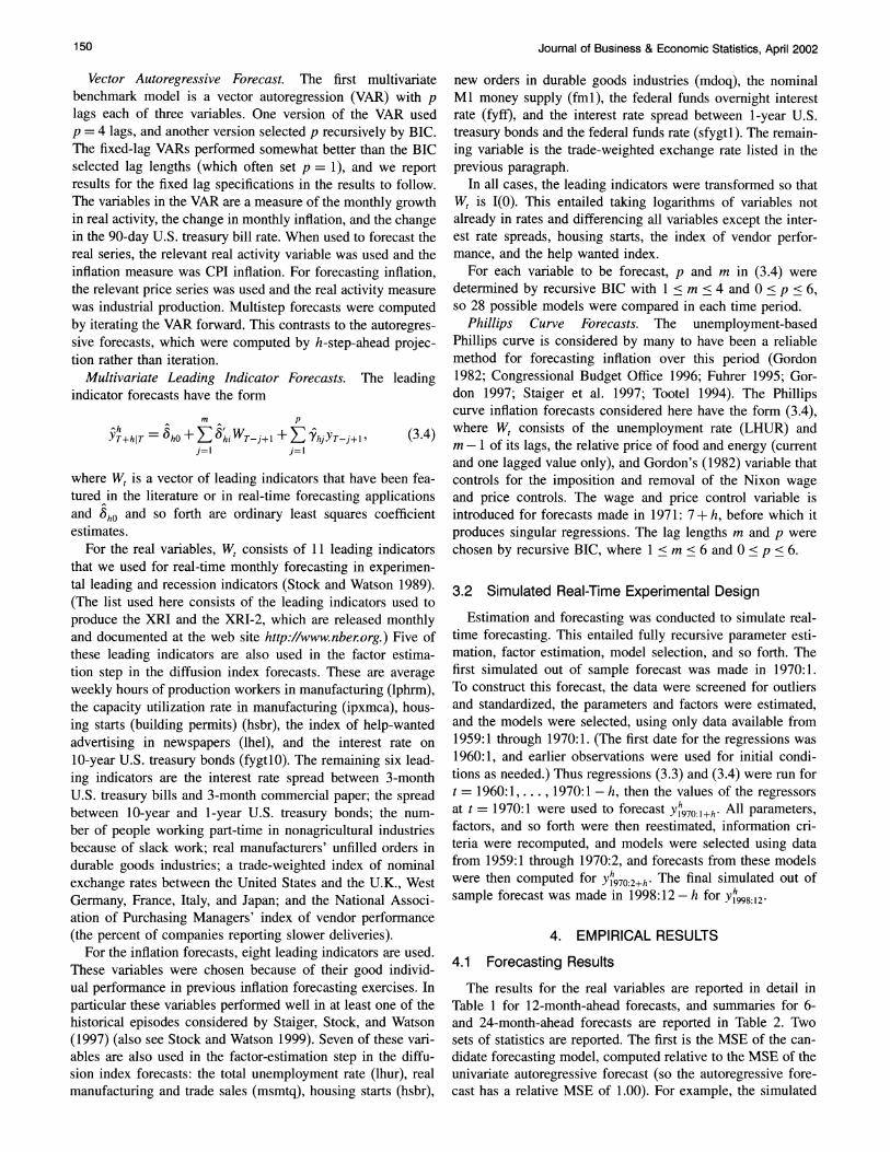
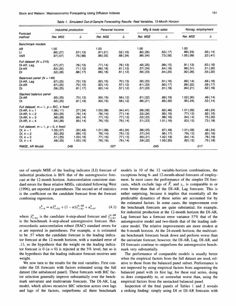
The results for the real variables are reported in detail in Table 1 for 12-month-ahead forecasts, and summaries for 6- and 24-month-ahead forecasts are reported in Table 2. Two sets of statistics are reported. The first is the MSE of the candidate forecasting model, computed relative to the MSE of the univariate autoregressive forecast (so the autoregressive forecast has a relative MSE of 1.00). For example, the simulated


Table 1. Simulated Out-of-Sample Forecasting Results: Real Variables, 12-Month Horizon

Industrial production Personal income Mfg & trade sales Nonag. employment Forecast method Rel. MSE & Rel. MSE & Rel. MSE & Rel. MSE &

Benchmark models AR 1.00 1.00 1.00 1.00 LI .86 (.27) .57(.13) .97(.21) .52(.15) .82(.25) .63(.17) .89 (.23) .56(.14) VAR .97 (.07) .75(.68) .98(.05) .68 (.34) .98(.04) .73(.58) 1.05(.09) .22 (.41)

Full dataset (N = 215) DI-AR, Lag .57(.27) .76(.13) .77(.14) .76(.13) .48(.25) .99(.15) .91 (.13) .63(.18) DI-AR .63(.25) .71 (.12) .86(.16) .61 (.12) .57(.24) .84(.18) .99(.31) .51 (.20) DI .52 (.26) .88(.17) .86(.16) .61 (.12) .56 (.23) .94 (.20) .92 (.26) .55 (.20)

Balanced panel (N = 149) DI-AR, Lag .67(.25) .70(.13) .82(.15) .70(.13) .56(.23) .91(.16) .88(.14) .68(.18) DI-AR .67 (.25) .70(.12) .92(.14) .57(.12) .61 (.23) .80(.17) .88(.22) .58 (.17) DI .59(.25) .81 (.17) .92(.14) .57 (.12) .57(.23) .91 (.18) .84(.21) .62 (.16)

Stacked balance panel DI-AR .65(.25) .70(.12) .93(.15) .56(.12) .61 (.22) .89(.19) 1.02(.30) .49(.14) DI .62(.25) .81 (.18) .93(.15) .56(.12) .66(.21) .85(.20) .95(.24) .53(.14)

Full dataset; m = 1, p = BIC, k fixed DI-AR, k= 1 1.06(.11) .27(.34) 1.03(.08) .34(.41) .98(.06) .63(.46) 1.01 (.09) .49(.24) DI-AR, k=2 .63(.25) .76(.14) .78(.14) .77(.14) .53(.24) .93(.15) .77(.13) .82(.15) DI-AR, k= 3 .56(.26) .84(.14) .77(.15) .77 (.13) .52(.23) .99(.16) .84(.14) .75(.20) DI-AR, k = 4 .54(.26) .85(.14) .76(.15) .78 (.14) .51 (.23) 1.01 (.16) .83(.15) .73 (.19)

Full dataset; m = 1, p = O, k fixed DI, k= 1 1.03(.07) .30(.49) 1.01 (.09) .46 (.34) .98(.05) .67 (.49) 1.01 (.09) .48 (.24) DI, k=2 .55(.25) .89(.15) .78(.14) .76 (.13) .57(.24) .95(.17) .78(.13) .83(.16) DI, k=3 .51(.25) 1.00(.16) .77(.15) .77 (.13) .60(.21) 1.02(.19) .84(.14) .76(.19) DI, k= 4 .49(.25) 1.00(.16) .76(.15) .78(.14) .59(.22) 1.03(.20) .82(.15) .75(.18)

RMSE, AR Model .049 .027 .045 .017

out of sample MSE of the leading indicator (LI) forecast of industrial production is 86% that of the autoregressive forecast at the 12-month horizon. Autocorrelation consistent standard errors for these relative MSEs, calculated following West

(1996), are reported in parentheses. The second set of statistics is the coefficient on the candidate forecast from the forecast combining regression,

h hh A(+hI ahAR h (4.1) Yt+h " oyt+hlt- Yt+hlt -ut+h

where ,+h is the candidate h-step-ahead forecast and Yh, AR

is the benchmark h-step-ahead autoregressive forecast. Het- eroscedastic autocorrelation robust (HAC) standard errors for a are reported in parentheses. For example, a is estimated to be .57 when the candidate forecast is the leading indicator forecast at the 12-month horizon, with a standard error of .13, so the hypothesis that the weight on the leading indicator forecast is 0 (a = 0) is rejected at the 5% level, but so is the hypothesis that the leading indicator forecast receives unit weight.

We now turn to the results for the real variables. First consider the DI forecasts with factors estimated using the full dataset (the unbalanced panel). These forecasts with BIC factor selection generally improve substantially over the benchmark univariate and multivariate forecasts. The DI-AR, Lag model, which allows recursive BIC selection across own lags and lags of the factors, outperforms all three benchmark

models in 10 of the 12 variable-horizon combinations, the exceptions being 6- and 12-month-ahead forecasts of employment. In most cases the performance of the simpler DI forecasts, which exclude lags of F, and y, is comparable to or even better than that of the DI-AR, Lag forecasts. This is rather surprising, because it implies that essentially all the predictable dynamics of these series are accounted for by the estimated factors. In some cases, the improvement over the benchmark forecasts are quite substantial; for example, for industrial production at the 12-month horizon the DI-AR, Lag forecast has a forecast error variance 57% that of the autoregressive model and two-thirds that of the leading indicator model. The relative improvements are more modest at the 6-month horizon. At the 24-month horizon, the multivariate benchmark forecasts break down and perform worse than the univariate forecast; however, the DI-AR, Lag, DI-AR, and DI forecasts continue to outperform the autoregressive benchmark very substantially.

The performance of comparable models is usually better when the empirical factors from the full dataset are used, relative to those from the balanced panel subset. Performance is not improved by using empirical factors from augmenting the balanced panel with its first lag; for these real series, doing so does comparably to, or somewhat worse than, using the empirical factors from the unstacked balanced panel.

Inspection of the final panels of Tables 1 and 2 reveals a striking finding: simply using DI or DI-AR forecasts with


Table 2. Simulated Out-of-Sample Forecasting Results: Real Variables, 6- and 24-Month Horizons

Industrial production Personal income Mfg & trade sales Nonag. employment Forecast method Rel. MSE & Rel. MSE & Rel. MSE & Rel. MSE &

A. Horizon = 6 months Benchmark models AR 1.00 1.00 1.00 1.00 LI .70(.25) .68(.13) .83(.15) .64(.11) .77(.19) .68(.14) .75(.19) .67(.12) VAR 1.01 (.05) .43 (.39) .99(.03) .63(.43) .99(.04) .64 (.45) 1.06(.07) .12(.34)

Full dataset (N = 215) DI-AR, Lag .69(.25) .69(.14) .77(.12) .86(.15) .63(.18) .89(.17) .94(.16) .56(.18) DI-AR .77(.30) .62(.16) .81 (.16) .66(.13) .70(.20) .76 (.17) 1.02(.32) .49(.19) DI .74(.25) .68 (.17) .81 (.16) .65(.13) .67(.20) .79(.18) .96(.28) .52(.19)

Balanced panel (N = 149) DI-AR, Lag .73 (.25) .68 (.16) .79(.13) .78(.13) .66(.17) .87(.17) .93(.17) .58(.21) DI-AR .78(.28) .62 (.16) .81 (.15) .66(.11) .76(.19) .70(.17) .97(.28) .52(.19) DI .73(.24) .69(.1(.15) .66(.11) .68(.19) .81 (.17) .95(.26) .53(.18)

Full dataset; m = 1, p = BIC, k fixed DI-AR, k= 1 .97(.15) .58 (.33) .91 (.07) .80(.23) .99(.11) .52 (.29) .94(.12) .60(.19) DI-AR, k=2 .67(.22) .77(.15) .76(.11) .90(.14) .64(.18) .86(.16) .84(.13) .71(.16) DI-AR, k=3 .64(.23) .81 (.15) .75(.12) .89(.14) .64(.18) .88(.17) .88(.14) .66(.17) DI-AR, k = 4 .64(.23) .80 (.15) .74(.13) .87(.14) .63(.18) .87(.15) .91 (.16) .60(.18)

RMSE, AR Model .030 .016 .028 .008

B. Horizon = 24 months Benchmark models AR 1.00 1.00 1.00 1.00 LI 1.09(.28) .45(.14) 1.29(.31) .30(.20) 1.08(.21) .45(.14) 1.07(.31) .47(.15) VAR 1.01 (.10) .44(.48) .98(.06) .63(.34) 1.03(.06) .13(.85) 1.06(.13) .35(.31)

Full dataset (N = 215) DI-AR, Lag .57 (.24) .88 (.13) .70(.20) .94(.23) .66(.18) .95 (.18) .82(.15) .88(.26) DI-AR .59(.25) .88 (.15) .76(.22) .80(.26) .70(.20) .89 (.19) .74(.19) .97 (.24) DI .55(.26) .91 (.14) .76(.22) .80(.25) .70(.20) .89(.19) .74(.19) .97 (.24)

Balanced panel (N = 149) DI-AR, Lag .57(.25) .87 (.14) .76(.19) .86(.23) .64(.20) .94(.18) .74(.17) 1.06(.25) DI-AR .58(.25) .87 (.14) .83(.20) .74(.24) .67(.19) .93 (.18) .76(.18) .94(.25) DI .58(.25) .87(.14) .83(.20) .74(.24) .67 (.20) .94(.19) .75(.18) .94(.24)

Full dataset; m = 1, p = BIC, k fixed DI-AR, k= 1 1.12(.19) .10(.46) 1.07(.09) .81(1.00) .97(.04) .90(.62) 1.03(.07) .33(.46) DI-AR, k= 2 .76(.19) .68(.11) .88(.13) .68(.17) .65(.20) .87 (.14) .72(.16) .99(.17) DI-AR, k=3 .58(.24) .89(.13) .72(.19) .90(.18) .70(.17) .89(.14) .79(.16) .95(.24) DI-AR, k= 4 .56(.24) .90(.14) .70(.20) .93(.23) .67(.18) .95(.18) .78(.16) .96(.24)

RMSE, AR Model .075 .046 .070 .031

two factors captures most of the forecasting improvement. In most cases, incorporating BIC factor and lag order selection provides little or no improvement over just using two factors, with no lags of the factors and no lagged dependent variables.

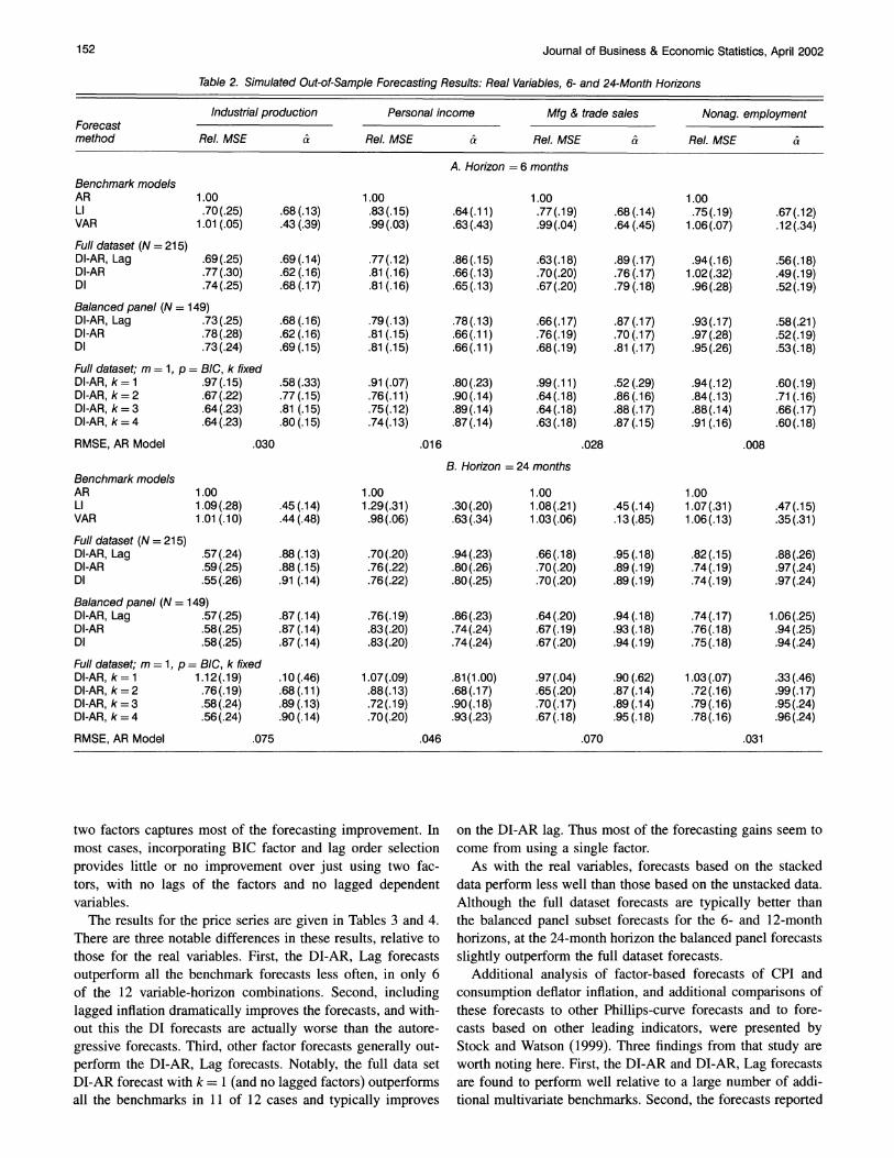
The results for the price series are given in Tables 3 and 4. There are three notable differences in these results, relative to those for the real variables. First, the DI-AR, Lag forecasts

outperform all the benchmark forecasts less often, in only 6 of the 12 variable-horizon combinations. Second, including lagged inflation dramatically improves the forecasts, and without this the DI forecasts are actually worse than the autoregressive forecasts. Third, other factor forecasts generally outperform the DI-AR, Lag forecasts. Notably, the full data set DI-AR forecast with k = 1 (and no lagged factors) outperforms all the benchmarks in 11 of 12 cases and typically improves

on the DI-AR lag. Thus most of the forecasting gains seem to come from using a single factor.

As with the real variables, forecasts based on the stacked data perform less well than those based on the unstacked data. Although the full dataset forecasts are typically better than the balanced panel subset forecasts for the 6- and 12-month horizons, at the 24-month horizon the balanced panel forecasts slightly outperform the full dataset forecasts.

Additional analysis of factor-based forecasts of CPI and

consumption deflator inflation, and additional comparisons of these forecasts to other Phillips-curve forecasts and to forecasts based on other leading indicators, were presented by Stock and Watson (1999). Three findings from that study are worth noting here. First, the DI-AR and DI-AR, Lag forecasts are found to perform well relative to a large number of additional multivariate benchmarks. Second, the forecasts reported


Table 3. Simulated Out-of-Sample Forecasting Results: Price Inflation, 12-Month Horizon

CPI Consumption deflator CPI exc. food & energy Producer price index Forecast method Rel. MSE & Rel. MSE & Rel. MSE & Rel. MSE &

Benchmark models AR 1.00 1.00 1.00 1.00 LI .79(.15) .76(.15) .95(.12) .58(.17) 1.00(.16) .50(.21) .82(.15) .75(.19) Phillips Curve .82(.13) .95(.20) .92(.10) .72(.23) .79(.18) .80(.22) .87(.14) .96(.30) VAR .91 (.09) .74(.20) 1.02(.06) .45(.20) .99 (.05) .56(.21) 1.29(.14) .25(.12)

Full dataset (N = 215) DI-AR, Lag .72(.14) .91 (.14) .90(.09) .65(.13) .84(.15) .76(.20) .83(.13) .78(.21) DI-AR .71 (.16) .83(.13) .90(.10) .62(.13) .85(.15) .74(.20) .82(.14) .75(.20) DI 1.30(.16) .34(.08) 1.40(.16) .25(.08) 1.55(.31) .24(.06) 2.40(.88) .13(.07)

Balanced panel (N = 149) DI-AR, Lag .70(.14) .94(.12) .90 (.08) .67(.15) .84(.15) .77(.21) .86(.11) .77(.21) DI-AR .69(.15) .88(.13) .87(.10) .66(.12) .85(.15) .73(.20) .85(.14) .71 (.19) DI 1.30(.16) .32(.08) 1.34(.13) .26(.09) 1.57(.33) .20(.07) 2.44(.87) .14(.06)

Stacked balance panel DI-AR .73(.15) .82(.12) .87(.09) .65(.12) .85(.15) .77(.21) .81 (.14) .75 (.20) DI 1.54(.31) .28(.08) 1.51 (.18) .25(.08) 1.55(.32) .23(.06) 3.06(1.89) .11 (.06)

Full dataset; m = 1, p = BIC, k fixed DI-AR, k= 1 .64(.15) 1.14(.14) .77(.12) .96(.16) .71 (.17) 1.25(.23) .76(.16) .95(.24) DI-AR, k=2 .67(.14) 1.07(.13) .83(.09) .83(.14) .72(.17) .97(.19) .77(.15) .93(.23) DI-AR, k=3 .76(.13) .91 (.15) .94(.07) .61 (.14) .86(.14) .73(.20) .86(.11) .78(.21) DI-AR, k = 4 .74(.14) .89(.15) .91 (.09) .64(.14) .87(.15) .72(.21) .82(.13) .79(.21)

Full dataset; m = 1, p = 0, k fixed DI, k= 1 1.60(.34) .25(.07) 1.56(.20) .22(.09) 1.55(.31) .23(.06) 2.76(1.61) .12(.07) DI, k=2 1.56(.31) .26(.07) 1.58(.20) .21 (.08) 1.62(.39) .22(.07) 2.72(1.56) .13(.07) DI, k=3 1.57(.32) .24(.08) 1.60(.20) .17(.08) 1.69(.43) .18(.07) 2.68(1.49) .13(.07) DI, k=4 1.56(.25) .25(.07) 1.56(.19) .21(.08) 1.67(.40) .19(.07) 2.55(.99) .16(.06)

RMSE, AR Model .021 .015 .019 .033

here can be further improved on using a single-factor forecast, where the factor is computed from a set of variables that measure only real economic activity. Forecasts based on this real economic activity factor have MSEs approximately 10% less than the best forecasts reported in Table 3. Finally, similar rankings of methods are obtained using I(1) forecasting models, rather than the 1(2) models used here, that is, when first rather than second differences of log prices are used for the forecasting equation and factor estimation.

In interpreting these results, it should be stressed that the multivariate leading indicator models are sophisticated forecasting tools that provide a stiff benchmark against which to judge the diffusion index forecasts. In our judgment, the performance of the leading indicator models reported here overstates their true potential out of sample performance, because the lists of leading indicators used to construct the forecasts were chosen by model selection methods based on their forecasting performance over the past two decades, as discussed in Section 3. In this light, we consider the performance of the various diffusion index models to be particularly encouraging.

4.2 Empirical Factors

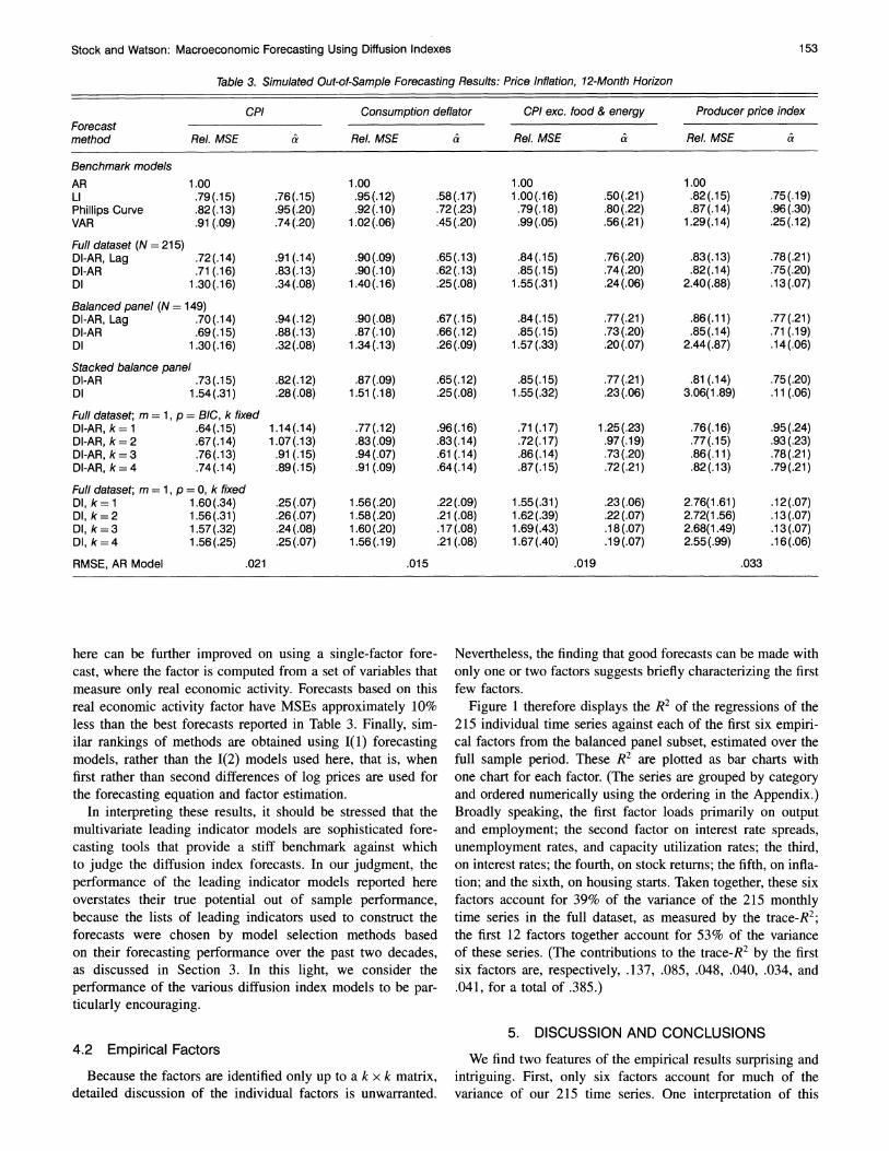
Because the factors are identified only up to a k x k matrix, detailed discussion of the individual factors is unwarranted.

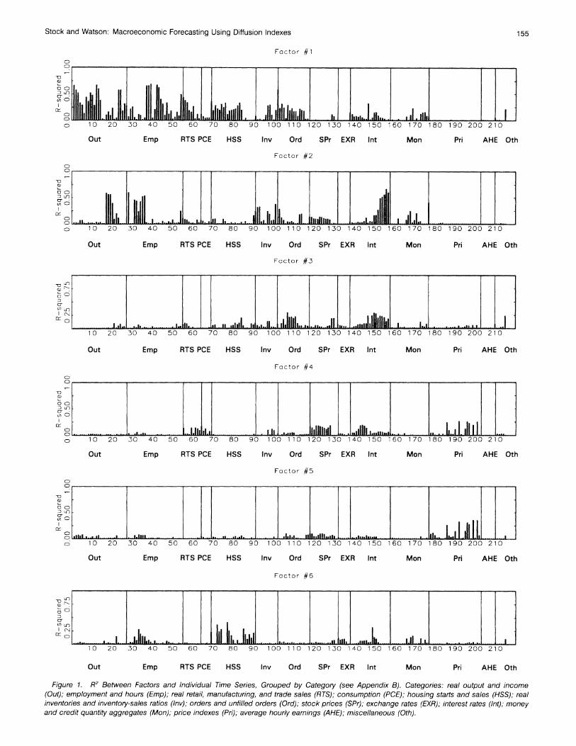
Nevertheless, the finding that good forecasts can be made with only one or two factors suggests briefly characterizing the first few factors.

Figure 1 therefore displays the R2 of the regressions of the 215 individual time series against each of the first six empirical factors from the balanced panel subset, estimated over the full sample period. These R2 are plotted as bar charts with one chart for each factor. (The series are grouped by category and ordered numerically using the ordering in the Appendix.) Broadly speaking, the first factor loads primarily on output and employment; the second factor on interest rate spreads, unemployment rates, and capacity utilization rates; the third, on interest rates; the fourth, on stock returns; the fifth, on inflation; and the sixth, on housing starts. Taken together, these six factors account for 39% of the variance of the 215 monthly time series in the full dataset, as measured by the trace-R2; the first 12 factors together account for 53% of the variance of these series. (The contributions to the trace-R2 by the first six factors are, respectively, .137, .085, .048, .040, .034, and .041, for a total of .385.)

5. DISCUSSION AND CONCLUSIONS

We find two features of the empirical results surprising and intriguing. First, only six factors account for much of the variance of our 215 time series. One interpretation of this


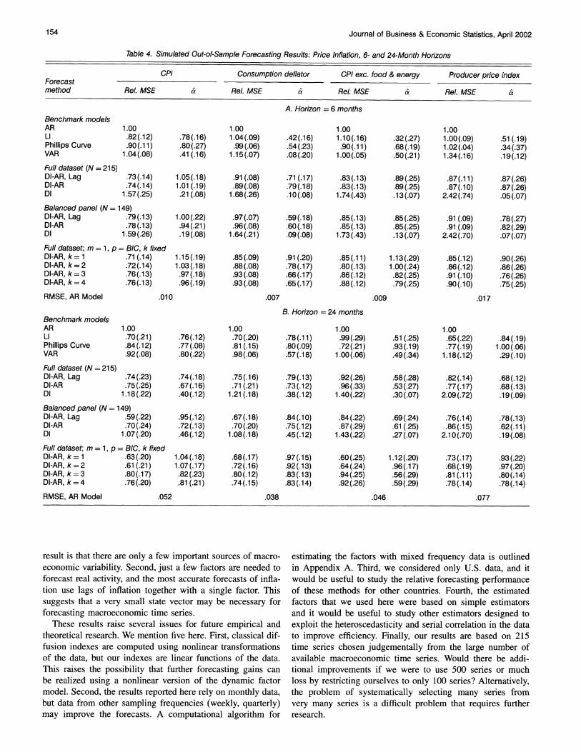
Table 4. Simulated Out-of-Sample Forecasting Results: Price Inflation, 6- and 24-Month Horizons

CPI Consumption deflator CPI exc. food & energy Producer price index Forecast method Rel. MSE & Rel. MSE & Rel. MSE & Rel. MSE &

A. Horizon = 6 months Benchmark models AR 1.00 1.00 1.00 1.00 LI .82(.12) .78(.16) 1.04(.09) .42(.16) 1.10(.16) .32(.27) 1.00(.09) .51(.19) Phillips Curve .90(.11) .80(.27) .99(.06) .54(.23) .90(.11) .68(.19) 1.02(.04) .34(.37) VAR 1.04(.08) .41(.16) 1.15(.07) .08(.20) 1.00(.05) .50(.21) 1.34(.16) .19(.12) Full dataset (N = 215) DI-AR, Lag .73(.14) 1.05(.18) .91 (.08) .71(.17) .83(.13) .89(.25) .87(.11) .87(.26) DI-AR .74(.14) 1.01(.19) .89(.08) .79(.18) .83(.13) .89(.25) .87(.10) .87(.26) DI 1.57(.25) .21(.08) 1.68(.26) .10(.08) 1.74(.43) .13(.07) 2.42(.74) .05(.07)

Balanced panel (N = 149) DI-AR, Lag .79(.13) 1.00(.22) .97(.07) .59(.18) .85(.13) .85(.25) .91 (.09) .78(.27) DI-AR .78(.13) .94(.21) .96(.08) .60(.18) .85(.13) .85(.25) .91 (.09) .82(.29) DI 1.59(.26) .19(.08) 1.64(.21) .09(.08) 1.73(.43) .13(.07) 2.42(.70) .07(.07) Full dataset; m = 1, p = BIC, k fixed DI-AR, k= 1 .71 (.14) 1.15(.19) .85(.09) .91(.20) .85(.11) 1.13(.29) .85(.12) .90(.26) DI-AR, k=2 .72(.14) 1.03(.18) .88(.08) .78(.17) .80(.13) 1.00(.24) .86(.12) .86(.26) DI-AR, k=3 .76(.13) .97(.18) .93(.08) .66(.17) .86(.12) .82(.25) .91(.10) .76(.26) DI-AR, k=4 .76(.13) .96(.19) .93(.08) .65(.17) .88(.12) .79(.25) .90(.10) .75(.25)

RMSE, AR Model .010 .007 .009 .017

B. Horizon = 24 months Benchmark models AR 1.00 1.00 1.00 1.00 LI .70(.21) .76(.12) .70(.20) .78(.11) .99(.29) .51(.25) .65(.22) .84(.19) Phillips Curve .84(.12) .77(.08) .81(.15) .80(.09) .72(.21) .93(.19) .77(.19) 1.00(.06) VAR .92(.08) .80(.22) .98(.06) .57(.18) 1.00(.06) .49(.34) 1.18(.12) .29(.10) Full dataset (N = 215) DI-AR, Lag .74(.23) .74(.18) .75(.16) .79(.13) .92(.26) .58(.28) .82(.14) .68(.12) DI-AR .75(.25) .67(.16) .71(.21) .73(.12) .96(.33) .53(.27) .77(.17) .68(.13) DI 1.18(.22) .40(.12) 1.21(.18) .38(.12) 1.40(.22) .30(.07) 2.09(.72) .19(.09)

Balanced panel (N = 149) DI-AR, Lag .59(.22) .95(.12) .67(.18) .84(.10) .84(.22) .69(.24) .76(.14) .78(.13) DI-AR .70(.24) .72(.13) .70(.20) .75(.12) .87(.29) .61 (.25) .86(.15) .62(.11) DI 1.07(.20) .46(.12) 1.08(.18) .45(.12) 1.43(.22) .27(.07) 2.10(.70) .19(.08)

Full dataset; m = 1, p = BIC, k fixed DI-AR, k= 1 .63(.20) 1.04(.18) .68(.17) .97(.15) .60(.25) 1.12(.20) .73(.17) .93(.22) DI-AR, k=2 .61(.21) 1.07(.17) .72(.16) .92(.13) .64(.24) .96(.17) .68(.19) .97(.20) DI-AR, k=3 .80(.17) .82(.23) .80(.12) .83(.13) .94(.25) .56(.29) .81(.11) .80(.14) DI-AR, k=4 .76(.20) .81(.21) .74(.15) .83(.14) .92(.26) .59(.29) .78(.14) .78(.14)

RMSE, AR Model .052 .038 .046 .077

result is that there are only a few important sources of macroeconomic variability. Second, just a few factors are needed to forecast real activity, and the most accurate forecasts of inflation use lags of inflation together with a single factor. This suggests that a very small state vector may be necessary for forecasting macroeconomic time series.

These results raise several issues for future empirical and theoretical research. We mention five here. First, classical diffusion indexes are computed using nonlinear transformations of the data, but our indexes are linear functions of the data. This raises the possibility that further forecasting gains can be realized using a nonlinear version of the dynamic factor model. Second, the results reported here rely on monthly data, but data from other sampling frequencies (weekly, quarterly) may improve the forecasts. A computational algorithm for

estimating the factors with mixed frequency data is outlined in Appendix A. Third, we considered only U.S. data, and it would be useful to study the relative forecasting performance of these methods for other countries. Fourth, the estimated factors that we used here were based on simple estimators and it would be useful to study other estimators designed to exploit the heteroscedasticity and serial correlation in the data to improve efficiency. Finally, our results are based on 215 time series chosen judgementally from the large number of available macroeconomic time series. Would there be additional improvements if we were to use 500 series or much loss by restricting ourselves to only 100 series? Alternatively, the problem of systematically selecting many series from very many series is a difficult problem that requires further research.


Factor #1 0

0o CD

CD:lull., .. .. ..

0 10 20 30 40 50 60 70 80 90 100 110 120 130 140 150 160 170 180 190 200 210

Out Emp RTS PCE HSS Inv Ord SPr EXR Int Mon Pri AHE Oth

Factor #2 CD C

00C)

C 10 20 30 40 50 60 70 80 90 100 110 120 130 140 150 160 170 180 190 200 210


Factor #3

Ll

II,, 0 . . ... ...C. ... Ii. J..lI.. II .... I, . II .....lL zL IIi...__ , L I_,,,, . a .... ........ I50 J.1 ..I ..i .... ..

10 20 30 40 50 60 70 80 90 100 11020 0 130 140 150 160 170 180 190 200 210


Factor #4 CD

10 20 30 40 50 60 70 80 90 100 110 120 130 140 150 160 170 180 190 200 210


Factor #4

L-i oCD

o CT I

.0 10 20 30 40 50 60 70 80 90 100 110 120 130 140 150 160 170 180 190 200 210


Factor #5 CD C

_5 L)

C 10 20 30 40 50 60 70 80 90 100 110 120 130 140 150 160 170 180 190 200 210


and credit quantity aggregates (Mon); price indexes (Pri); average hourly earnings (AHE); miscellaneous (0th).


ACKNOWLEDGMENTS

The material in this article originally appeared in our paper titled "Diffusion Indexes." We thank Michael Boldin, Frank Diebold, Gregory Chow, Andrew Harvey, Lucrezia Reichlin, Ken Wallis, Charles Whiteman, and several referees for help- ful discussions and comments and Lewis Chan and Alexei Onatski for skilled research assistance. This research was sup- ported in part by National Science Foundation grants SBR- 9409629 and SBR-9730489.

APPENDIX A: EM ESTIMATION WITH AN UNBALANCED PANEL AND DATA IRREGULARITIES

In practice, when N is large one encounters various data irregularities, including occasionally missing observations, unbalanced panels, and mixed frequency (for example, monthly and quarterly) data. In this case, a modification of standard principal component estimation is necessary. To motivate the modification, consider the least squares estimators of A and F, from (2.4) from a balanced panel. The objective function is

N T

V(F, A) = E E(Xit -AiF,)2, (A.1) i=1 t=1

where Ai is the ith row of A. (A.1) can be minimized by the usual eigenvalue calculations and F, are the principal components of X,.

When the panel is unbalanced, least squares estimators of F, can be calculated from the objective function

NT

Vt(F, A) = = li,(Xi, - -AF,)2, (A.2)

i=1 t=l

where li, = 1 if Xi, is available and 0 otherwise. Minimization of (A.2) requires iterative methods. This appendix summarizes an iterative method based on the EM algorithm that has proved to be easy and effective.

To motivate this EM algorithm, notice that V(F, A) is pro- portional to the log-likelihood under the assumption that Xi, are iid N(A'F,, 1), in which case the least squares estimators are the Gaussian maximum likelihood estimators. Because Vt is just a missing data version of V and because minimization of V is computationally simple, a simple EM algorithm can be constructed to minimize Vt.

The jth iteration of the algorithm is defined as follows. Let A and F denote estimates of A and F constructed from the (j- 1)st iteration, and let

Q(Xt, F, A, F, A) = E•,[V(F, A) I Xt], (A.3)

where Xt denotes the full set of observed data and

E;i[V(F, A) IXt] is the expected value of the complete data log-likelihood V(F, A), evaluated using the conditional den- sity of X IXt evaluated at F and A. The estimates of F and A at iteration j solve MinF, AQ(Xt, F, A, F, A).

To carry out the calculations, note that

Q(Xt, F, A, F, A)

= Z Z{Ef•7(xt I Xt) + (AF,)2 - 2it(A'Ft)}, (A.4) i t

where Xi, = E• •(Xi, I Xt). The first term on the right side of

(A.4) does not depend on F or A, and so for purposes of minimization it can be replaced by Ei L E 7t. This implies that the values of F and A that minimize (A.4) can be calculated as the minimizers of V(F, A) = Ei Z,(Xi, - A•F,)2. At the jth step, this reduces to the usual principal component eigenvalue calculation where the missing data are replaced by their

expectation conditional on the observed data and using the parameter values from the previous iteration. If the full dataset contains a subset that constitutes a balanced panel, then start- ing values for F in the EM iteration can be obtained using estimates from the balanced panel subset.

We now provide some additional details on the calculation of Xit, for some important special cases. Let Xi =

(Xi ..., Xi)', and let Xt be the vector of observations on the ith variable. Suppose that Xt = AiX, for some known matrix

Ai, as can be done in the cases of missing values and tempo- ral aggregation, for example. Then E(Xi I Xt) = E(X I Xt) = FAi + A'(AiA')-(Xt -

AiFAi), where (AiA)- is the generalized inverse of AiAi. The particulars of these calculations are now presented for some important special cases. In the first four special cases discussed, this level of generality is unnec- essary and the formula for Xit follows quite simply from the nature of the data irregularity.

A. Missing Observations. Suppose some observations on

Xi, are missing. Then, during iteration j, the elements of the estimated balanced panel are constructed as Xi, = Xit if

Xi, observed and Xi = AiF, otherwise. The estimate of F is then updated by computing the eigenvectors correspond- ing to the largest r eigenvalues of N-1 Ei XiXi, where Xi =

(Xi,9 Xi2 ..., XiT)'. The estimate of A is updated by the ordinary least squares regression of X onto this updated estimate of F.

B. Mixed Monthly and Quarterly Data-I(O) Stock Vari- ables. A series that is observed quarterly and is a stock variable would be the point-in-time level of a variable at the end of the quarter, say, the level of inventories at the end of the quarter. If this series is I(0), then it is handled as in case A; that is, it is treated as a monthly series with missing observations in the first and second months of the quarter.

C. Mixed Monthly and Quarterly Data--l(O) Flow Vari- ables. A quarterly flow variable is the average (or sum) of unobserved monthly values. If this series is I(0), it can be treated as follows. The unobserved monthly series, Xit, is measured only as the time aggregate Xiq, where Xq =

(1/3)(Xi, t_2 + Xi,_1 + Xi,) for t = 3, 6, 9, 12 ... and X, is missing for all other values of t. In this case estimation proceeds as in case A but with Xi, = AiF, + eit, where

ei, =

Xq, - Ai(F7-2 + F,_1 + F7)/3, where 7 = 3 when t = 1,2, 3, 7 = 6, when t = 4, 5, 6, and so forth.


D. Mixed Monthly and Quarterly Data--I(1) stock variables. Suppose that underlying monthly data are I(1) and let

X1i' denote the quarterly first difference stock variable, assumed to be measured in the third month of every quarter, and let

Xit denote the monthly first difference of the variable. Then X = (Xi, t2 + Xi, t-1 + X

it) for t - 3, 6, 9, 129 .... and X is

missing for all other values of t. In this case estimation proceeds as in case A but with Xit = AiFt + (1/3)eit, where it = X, - A'(Fi-2 + F,-1 + F), where 7 = 3 when t= 1, 2, 3, r = 6, when t = 4, 5, 6, and so forth.

E. Mixed Monthly and Quarterly Data--I(1) Flow Vari- ables. Construction of Xit is more difficult here than in the earlier cases. Here the general regression formula given above can be implemented after specifying Xj and Ai. Let the quarterly first differences be denoted by Xq, which is assumed to be observed at the end of every quarter. The vector of observations is then X= (Xq3, X9 ... .)', where denotes the month of the last quarterly observation. If the underlying quarterly data are averages of monthly series, and if the monthly first differences are denoted by Xit, then Xi, = (1/3)(Xi,t, + 2Xi, t_ + 3Xit-2 + 2Xit-3 + Xit-4) for t = 3, 6, 9, 12,..... and this implicitly defines the rows of Ai. Then the estimate of Xi is given by X. = FAi +A'(AiA>)-'(XI - AiFAi).

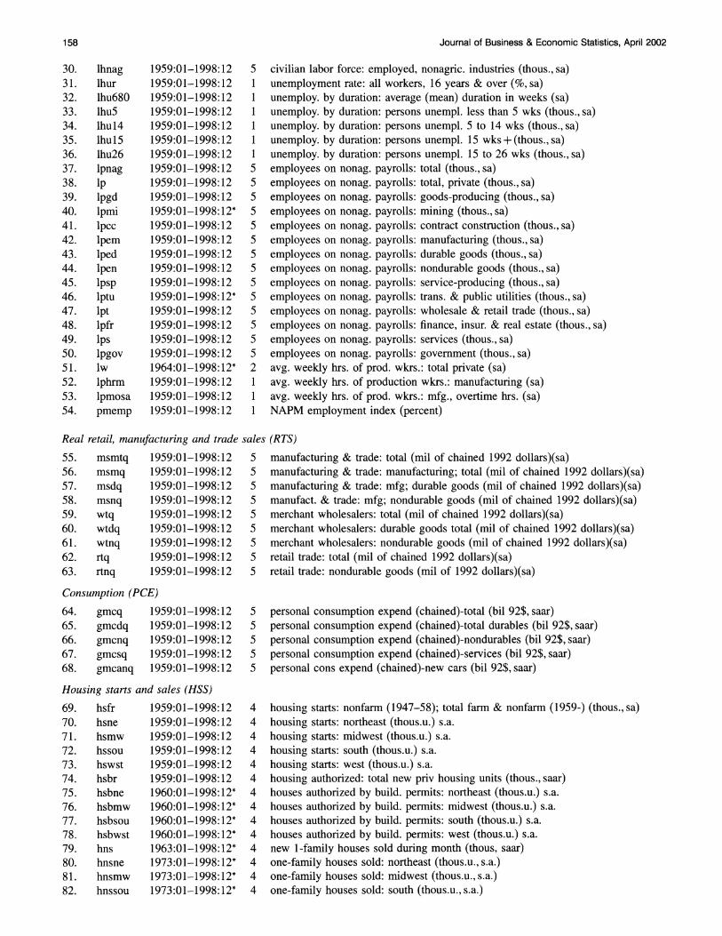
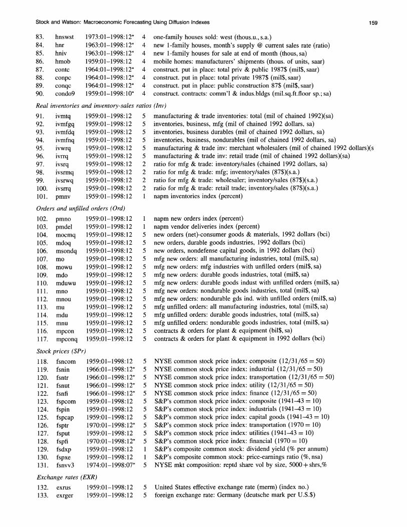
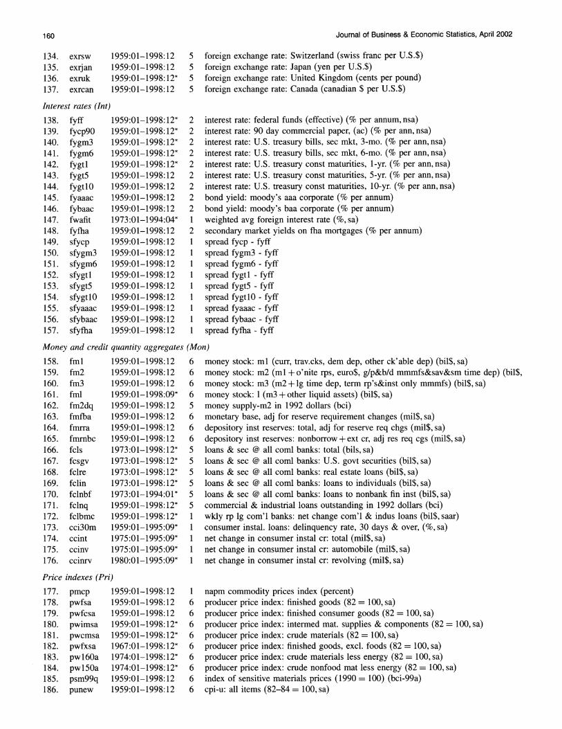
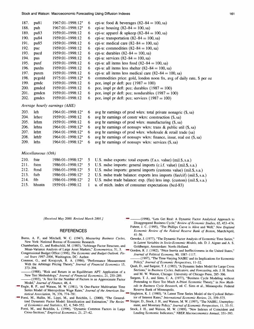
APPENDIX B: DATA DESCRIPTION

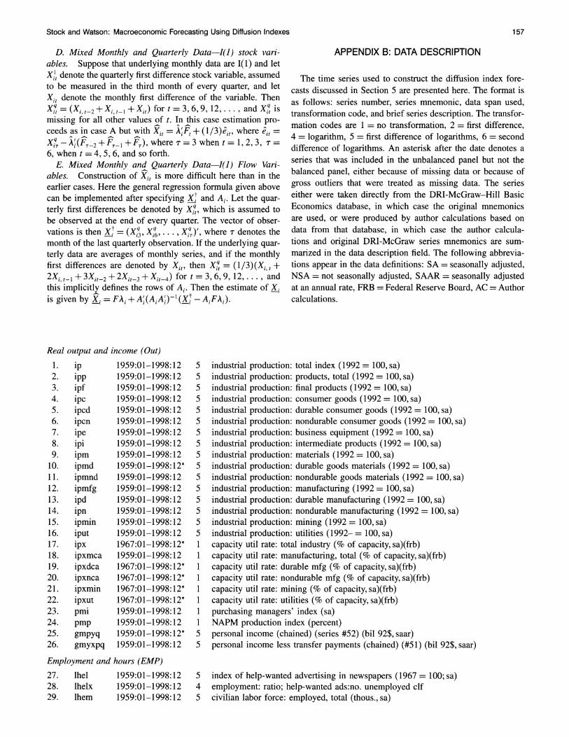
The time series used to construct the diffusion index forecasts discussed in Section 5 are presented here. The format is as follows: series number, series mnemonic, data span used, transformation code, and brief series description. The transformation codes are 1 = no transformation, 2 = first difference, 4 = logarithm, 5 = first difference of logarithms, 6 = second difference of logarithms. An asterisk after the date denotes a series that was included in the unbalanced panel but not the balanced panel, either because of missing data or because of gross outliers that were treated as missing data. The series either were taken directly from the DRI-McGraw-Hill Basic Economics database, in which case the original mnemonics are used, or were produced by author calculations based on data from that database, in which case the author calculations and original DRI-McGraw series mnemonics are summarized in the data description field. The following abbrevia- tions appear in the data definitions: SA = seasonally adjusted, NSA = not seasonally adjusted, SAAR = seasonally adjusted at an annual rate, FRB = Federal Reserve Board, AC = Author calculations.

Real output and income (Out) 1. ip 1959:01-1998:12 5 industrial production: total index (1992 = 100, sa) 2. ipp 1959:01-1998:12 5 industrial production: products, total (1992 = 100, sa) 3. ipf 1959:01-1998:12 5 industrial production: final products (1992 = 100, sa) 4. ipc 1959:01-1998:12 5 industrial production: consumer goods (1992 = 100, sa) 5. ipcd 1959:01-1998:12 5 industrial production: durable consumer goods (1992 = 100, sa) 6. ipcn 1959:01-1998:12 5 industrial production: nondurable consumer goods (1992 = 100, sa) 7. ipe 1959:01-1998:12 5 industrial production: business equipment (1992 = 100, sa) 8. ipi 1959:01-1998:12 5 industrial production: intermediate products (1992 = 100, sa) 9. ipm 1959:01-1998:12 5 industrial production: materials (1992 = 100, sa)

10. ipmd 1959:01-1998:12* 5 industrial production: durable goods materials (1992 = 100, sa) 11. ipmnd 1959:01-1998:12 5 industrial production: nondurable goods materials (1992 = 100, sa) 12. ipmfg 1959:01-1998:12 5 industrial production: manufacturing (1992 = 100, sa) 13. ipd 1959:01-1998:12 5 industrial production: durable manufacturing (1992 = 100, sa) 14. ipn 1959:01-1998:12 5 industrial production: nondurable manufacturing (1992 = 100, sa) 15. ipmin 1959:01-1998:12 5 industrial production: mining (1992 = 100, sa) 16. iput 1959:01-1998:12 5 industrial production: utilities (1992- = 100, sa) 17. ipx 1967:01-1998:12* 1 capacity util rate: total industry (% of capacity, sa)(frb) 18. ipxmca 1959:01-1998:12 1 capacity util rate: manufacturing, total (% of capacity, sa)(frb) 19. ipxdca 1967:01-1998:12* 1 capacity util rate: durable mfg (% of capacity, sa)(frb) 20. ipxnca 1967:01-1998:12* 1 capacity util rate: nondurable mfg (% of capacity, sa)(frb) 21. ipxmin 1967:01-1998:12* 1 capacity util rate: mining (% of capacity, sa)(frb) 22. ipxut 1967:01-1998:12* 1 capacity util rate: utilities (% of capacity, sa)(frb) 23. pmi 1959:01-1998:12 1 purchasing managers' index (sa) 24. pmp 1959:01-1998:12 1 NAPM production index (percent) 25. gmpyq 1959:01-1998:12* 5 personal income (chained) (series #52) (bil 92$, saar) 26. gmyxpq 1959:01-1998:12 5 personal income less transfer payments (chained) (#51) (bil 92$, saar)

Employment and hours (EMP) 27. lhel 1959:01-1998:12 5 index of help-wanted advertising in newspapers (1967 = 100; sa) 28. lhelx 1959:01-1998:12 4 employment: ratio; help-wanted ads:no. unemployed clf 29. lhem 1959:01-1998:12 5 civilian labor force: employed, total (thous., sa)


30. lhnag 1959:01-1998:12 5 civilian labor force: employed, nonagric. industries (thous., sa) 31. lhur 1959:01-1998:12 1 unemployment rate: all workers, 16 years & over (%, sa) 32. lhu680 1959:01-1998:12 1 unemploy. by duration: average (mean) duration in weeks (sa) 33. lhu5 1959:01-1998:12 1 unemploy. by duration: persons unempl. less than 5 wks (thous., sa) 34. lhul4 1959:01-1998:12 1 unemploy. by duration: persons unempl. 5 to 14 wks (thous., sa) 35. lhul5 1959:01-1998:12 1 unemploy. by duration: persons unempl. 15 wks + (thous., sa) 36. lhu26 1959:01-1998:12 1 unemploy. by duration: persons unempl. 15 to 26 wks (thous., sa) 37. lpnag 1959:01-1998:12 5 employees on nonag. payrolls: total (thous., sa) 38. lp 1959:01-1998:12 5 employees on nonag. payrolls: total, private (thous., sa) 39. lpgd 1959:01-1998:12 5 employees on nonag. payrolls: goods-producing (thous., sa) 40. lpmi 1959:01-1998:12* 5 employees on nonag. payrolls: mining (thous., sa) 41. lpcc 1959:01-1998:12 5 employees on nonag. payrolls: contract construction (thous., sa) 42. lpem 1959:01-1998:12 5 employees on nonag. payrolls: manufacturing (thous., sa) 43. lped 1959:01-1998:12 5 employees on nonag. payrolls: durable goods (thous., sa) 44. lpen 1959:01-1998:12 5 employees on nonag. payrolls: nondurable goods (thous., sa) 45. lpsp 1959:01-1998:12 5 employees on nonag. payrolls: service-producing (thous., sa) 46. lptu 1959:01-1998:12* 5 employees on nonag. payrolls: trans. & public utilities (thous., sa) 47. lpt 1959:01-1998:12 5 employees on nonag. payrolls: wholesale & retail trade (thous., sa) 48. lpfr 1959:01-1998:12 5 employees on nonag. payrolls: finance, insur. & real estate (thous., sa) 49. lps 1959:01-1998:12 5 employees on nonag. payrolls: services (thous., sa) 50. lpgov 1959:01-1998:12 5 employees on nonag. payrolls: government (thous., sa) 51. lw 1964:01-1998:12* 2 avg. weekly hrs. of prod. wkrs.: total private (sa) 52. lphrm 1959:01-1998:12 1 avg. weekly hrs. of production wkrs.: manufacturing (sa) 53. lpmosa 1959:01-1998:12 1 avg. weekly hrs. of prod. wkrs.: mfg., overtime hrs. (sa) 54. pmemp 1959:01-1998:12 1 NAPM employment index (percent)

Real retail, manufacturing and trade sales (RTS) 55. msmtq 1959:01-1998:12 5 manufacturing & trade: total (mil of chained 1992 dollars)(sa) 56. msmq 1959:01-1998:12 5 manufacturing & trade: manufacturing; total (mil of chained 1992 dollars)(sa) 57. msdq 1959:01-1998:12 5 manufacturing & trade: mfg; durable goods (mil of chained 1992 dollars)(sa) 58. msnq 1959:01-1998:12 5 manufact. & trade: mfg; nondurable goods (mil of chained 1992 dollars)(sa) 59. wtq 1959:01-1998:12 5 merchant wholesalers: total (mil of chained 1992 dollars)(sa) 60. wtdq 1959:01-1998:12 5 merchant wholesalers: durable goods total (mil of chained 1992 dollars)(sa) 61. wtnq 1959:01-1998:12 5 merchant wholesalers: nondurable goods (mil of chained 1992 dollars)(sa) 62. rtq 1959:01-1998:12 5 retail trade: total (mil of chained 1992 dollars)(sa) 63. rtnq 1959:01-1998:12 5 retail trade: nondurable goods (mil of 1992 dollars)(sa)

Consumption (PCE) 64. gmcq 1959:01-1998:12 5 personal consumption expend (chained)-total (bil 92$, saar) 65. gmcdq 1959:01-1998:12 5 personal consumption expend (chained)-total durables (bil 92$, saar) 66. gmcnq 1959:01-1998:12 5 personal consumption expend (chained)-nondurables (bil 92$, saar) 67. gmcsq 1959:01-1998:12 5 personal consumption expend (chained)-services (bil 92$, saar) 68. gmcanq 1959:01-1998:12 5 personal cons expend (chained)-new cars (bil 92$, saar)

Housing starts and sales (HSS)

69. hsfr 1959:01-1998:12 4 housing starts: nonfarm (1947-58); total farm & nonfarm (1959-) (thous.,sa) 70. hsne 1959:01-1998:12 4 housing starts: northeast (thous.u.) s.a. 71. hsmw 1959:01-1998:12 4 housing starts: midwest (thous.u.) s.a. 72. hssou 1959:01-1998:12 4 housing starts: south (thous.u.) s.a. 73. hswst 1959:01-1998:12 4 housing starts: west (thous.u.) s.a. 74. hsbr 1959:01-1998:12 4 housing authorized: total new priv housing units (thous., saar) 75. hsbne 1960:01-1998:12* 4 houses authorized by build, permits: northeast (thous.u.) s.a. 76. hsbmw 1960:01-1998:12* 4 houses authorized by build. permits: midwest (thous.u.) s.a. 77. hsbsou 1960:01-1998:12* 4 houses authorized by build. permits: south (thous.u.) s.a. 78. hsbwst 1960:01-1998:12* 4 houses authorized by build. permits: west (thous.u.) s.a. 79. hns 1963:01-1998:12* 4 new 1-family houses sold during month (thous, saar) 80. hnsne 1973:01-1998:12* 4 one-family houses sold: northeast (thous.u., s.a.) 81. hnsmw 1973:01-1998:12* 4 one-family houses sold: midwest (thous.u., s.a.) 82. hnssou 1973:01-1998:12* 4 one-family houses sold: south (thous.u., s.a.)


83. hnswst 1973:01-1998:12* 4 one-family houses sold: west (thous.u., s.a.) 84. hnr 1963:01-1998:12* 4 new 1-family houses, month's supply @ current sales rate (ratio) 85. hniv 1963:01-1998:12* 4 new 1-family houses for sale at end of month (thous, sa) 86. hmob 1959:01-1998:12 4 mobile homes: manufacturers' shipments (thous. of units, saar) 87. contc 1964:01-1998:12* 4 construct. put in place: total priv & public 1987$ (mil$, saar) 88. conpc 1964:01-1998:12* 4 construct. put in place: total private 1987$ (mil$, saar) 89. conqc 1964:01-1998:12* 4 construct. put in place: public construction 87$ (mil$, saar) 90. condo9 1959:01-1998:10* 4 construct. contracts: comm'l & indus.bldgs (mil.sq.ft.floor sp.; sa)

Real inventories and inventory-sales ratios (Inv) 91. ivmtq 1959:01-1998:12 5 manufacturing & trade inventories: total (mil of chained 1992)(sa) 92. ivmfgq 1959:01-1998:12 5 inventories, business, mfg (mil of chained 1992 dollars, sa) 93. ivmfdq 1959:01-1998:12 5 inventories, business durables (mil of chained 1992 dollars, sa) 94. ivmfnq 1959:01-1998:12 5 inventories, business, nondurables (mil of chained 1992 dollars, sa) 95. ivwrq 1959:01-1998:12 5 manufacturing & trade inv: merchant wholesalers (mil of chained 1992 dollars)(s 96. ivrrq 1959:01-1998:12 5 manufacturing & trade inv: retail trade (mil of chained 1992 dollars)(sa) 97. ivsrq 1959:01-1998:12 2 ratio for mfg & trade: inventory/sales (chained 1992 dollars, sa) 98. ivsrmq 1959:01-1998:12 2 ratio for mfg & trade: mfg; inventory/sales (87$)(s.a.) 99. ivsrwq 1959:01-1998:12 2 ratio for mfg & trade: wholesaler; inventory/sales (87$)(s.a.) 100. ivsrrq 1959:01-1998:12 2 ratio for mfg & trade: retail trade; inventory/sales (87$)(s.a.) 101. pmnv 1959:01-1998:12 1 napm inventories index (percent)

Orders and unfilled orders (Ord)

102. pmno 1959:01-1998:12 1 napm new orders index (percent) 103. pmdel 1959:01-1998:12 1 napm vendor deliveries index (percent) 104. mocmq 1959:01-1998:12 5 new orders (net)-consumer goods & materials, 1992 dollars (bci) 105. mdoq 1959:01-1998:12 5 new orders, durable goods industries, 1992 dollars (bci) 106. msondq 1959:01-1998:12 5 new orders, nondefense capital goods, in 1992 dollars (bci) 107. mo 1959:01-1998:12 5 mfg new orders: all manufacturing industries, total (mil$, sa) 108. mowu 1959:01-1998:12 5 mfg new orders: mfg industries with unfilled orders (mil$, sa) 109. mdo 1959:01-1998:12 5 mfg new orders: durable goods industries, total (mil$, sa) 110. mduwu 1959:01-1998:12 5 mfg new orders: durable goods indust with unfilled orders (mil$, sa) 111. mno 1959:01-1998:12 5 mfg new orders: nondurable goods industries, total (mil$, sa) 112. mnou 1959:01-1998:12 5 mfg new orders: nondurable gds ind. with unfilled orders (mil$, sa) 113. mu 1959:01-1998:12 5 mfg unfilled orders: all manufacturing industries, total (mil$, sa) 114. mdu 1959:01-1998:12 5 mfg unfilled orders: durable goods industries, total (mil$, sa) 115. mnu 1959:01-1998:12 5 mfg unfilled orders: nondurable goods industries, total (mil$, sa) 116. mpcon 1959:01-1998:12 5 contracts & orders for plant & equipment (bil$, sa) 117. mpconq 1959:01-1998:12 5 contracts & orders for plant & equipment in 1992 dollars (bci)

Stock prices (SPr) 118. fsncom 1959:01-1998:12 5 NYSE common stock price index: composite (12/31/65 = 50) 119. fsnin 1966:01-1998:12* 5 NYSE common stock price index: industrial (12/31/65 = 50) 120. fsntr 1966:01-1998:12* 5 NYSE common stock price index: transportation (12/31/65 = 50) 121. fsnut 1966:01-1998:12* 5 NYSE common stock price index: utility (12/31/65 = 50) 122. fsnfi 1966:01-1998:12* 5 NYSE common stock price index: finance (12/31/65 = 50) 123. fspcom 1959:01-1998:12 5 S&P's common stock price index: composite (1941-43 = 10) 124. fspin 1959:01-1998:12 5 S&P's common stock price index: industrials (1941-43 = 10) 125. fspcap 1959:01-1998:12 5 S&P's common stock price index: capital goods (1941--43 = 10) 126. fsptr 1970:01-1998:12" 5 S&P's common stock price index: transportation (1970 = 10) 127. fsput 1959:01-1998:12 5 S&P's common stock price index: utilities (1941-43 = 10) 128. fspfi 1970:01-1998:12* 5 S&P's common stock price index: financial (1970 = 10) 129. fsdxp 1959:01-1998:12 1 S&P's composite common stock: dividend yield (% per annum) 130. fspxe 1959:01-1998:12 1 S&P's composite common stock: price-earnings ratio (%, nsa) 131. fsnvv3 1974:01-1998:07* 5 NYSE mkt composition: reptd share vol by size, 5000 + shrs,%

Exchange rates (EXR)

132. exrus 1959:01-1998:12 5 United States effective exchange rate (merm) (index no.) 133. exrger 1959:01-1998:12 5 foreign exchange rate: Germany (deutsche mark per U.S.$)


134. exrsw 1959:01-1998:12 5 foreign exchange rate: Switzerland (swiss franc per U.S.$) 135. exrjan 1959:01-1998:12 5 foreign exchange rate: Japan (yen per U.S.$) 136. exruk 1959:01-1998:12* 5 foreign exchange rate: United Kingdom (cents per pound) 137. exrcan 1959:01-1998:12 5 foreign exchange rate: Canada (canadian $ per U.S.$)

Interest rates (Int) 138. fyff 1959:01-1998:12* 2 interest rate: federal funds (effective) (% per annum, nsa) 139. fycp90 1959:01-1998:12* 2 interest rate: 90 day commercial paper, (ac) (% per ann, nsa) 140. fygm3 1959:01-1998:12* 2 interest rate: U.S. treasury bills, sec mkt, 3-mo. (% per ann, nsa) 141. fygm6 1959:01-1998:12* 2 interest rate: U.S. treasury bills, sec mkt, 6-mo. (% per ann, nsa) 142. fygtl 1959:01-1998:12* 2 interest rate: U.S. treasury const maturities, 1-yr. (% per ann, nsa) 143. fygt5 1959:01-1998:12 2 interest rate: U.S. treasury const maturities, 5-yr. (% per ann, nsa) 144. fygtl0 1959:01-1998:12 2 interest rate: U.S. treasury const maturities, 10-yr. (% per ann, nsa) 145. fyaaac 1959:01-1998:12 2 bond yield: moody's aaa corporate (% per annum) 146. fybaac 1959:01-1998:12 2 bond yield: moody's baa corporate (% per annum) 147. fwafit 1973:01-1994:04* 1 weighted avg foreign interest rate (%, sa) 148. fyfha 1959:01-1998:12 2 secondary market yields on fha mortgages (% per annum) 149. sfycp 1959:01-1998:12 1 spread fycp - fyff 150. sfygm3 1959:01-1998:12 1 spread fygm3 - fyff 151. sfygm6 1959:01-1998:12 1 spread fygm6 - fyff 152. sfygtl 1959:01-1998:12 1 spread fygtl - fyff 153. sfygt5 1959:01-1998:12 1 spread fygt5 - fyff 154. sfygtl0 1959:01-1998:12 1 spread fygtl0 - fyff 155. sfyaaac 1959:01-1998:12 1 spread fyaaac - fyff 156. sfybaac 1959:01-1998:12 1 spread fybaac - fyff 157. sfyfha 1959:01-1998:12 1 spread fyfha - fyff

Money and credit quantity aggregates (Mon) 158. fml 1959:01-1998:12 6 money stock: ml (curr, trav.cks, dem dep, other ck'able dep) (bil$, sa) 159. fm2 1959:01-1998:12 6 money stock: m2 (ml + o'nite rps, euro$, g/p&b/d mmmfs&sav&sm time dep) (bil$, 160. fm3 1959:01-1998:12 6 money stock: m3 (m2 + Ig time dep, term rp's&inst only mmmfs) (bil$, sa) 161. fml 1959:01-1998:09* 6 money stock: 1 (m3 + other liquid assets) (bil$, sa) 162. fm2dq 1959:01-1998:12 5 money supply-m2 in 1992 dollars (bci) 163. fmfba 1959:01-1998:12 6 monetary base, adj for reserve requirement changes (mil$, sa) 164. fmrra 1959:01-1998:12 6 depository inst reserves: total, adj for reserve req chgs (mil$, sa) 165. fmrnbc 1959:01-1998:12 6 depository inst reserves: nonborrow + ext cr, adj res req cgs (mil$, sa) 166. fcls 1973:01-1998:12* 5 loans & sec @ all coml banks: total (bils, sa) 167. fcsgv 1973:01-1998:12* 5 loans & sec @ all coml banks: U.S. govt securities (bil$, sa) 168. fclre 1973:01-1998:12* 5 loans & sec @ all coml banks: real estate loans (bil$, sa) 169. fclin 1973:01-1998:12* 5 loans & sec @ all coml banks: loans to individuals (bil$, sa) 170. fclnbf 1973:01-1994:01* 5 loans & sec @ all coml banks: loans to nonbank fin inst (bil$, sa) 171. fclnq 1959:01-1998:12* 5 commercial & industrial loans outstanding in 1992 dollars (bci) 172. fclbmc 1959:01-1998:12* 1 wkly rp Ig com'l banks: net change com'l & indus loans (bil$, saar) 173. cci30m 1959:01-1995:09* 1 consumer instal. loans: delinquency rate, 30 days & over, (%, sa) 174. ccint 1975:01-1995:09* 1 net change in consumer instal cr: total (mil$, sa) 175. ccinv 1975:01-1995:09* 1 net change in consumer instal cr: automobile (mil$, sa) 176. ccinrv 1980:01-1995:09* 1 net change in consumer instal cr: revolving (mil$, sa)

Price indexes (Pri)

177. pmcp 1959:01-1998:12 1 napm commodity prices index (percent) 178. pwfsa 1959:01-1998:12 6 producer price index: finished goods (82 = 100, sa) 179. pwfcsa 1959:01-1998:12 6 producer price index: finished consumer goods (82 = 100, sa) 180. pwimsa 1959:01-1998:12* 6 producer price index: intermed mat. supplies & components (82 = 100, sa) 181. pwcmsa 1959:01-1998:12* 6 producer price index: crude materials (82 = 100, sa) 182. pwfxsa 1967:01-1998:12* 6 producer price index: finished goods, excl. foods (82 = 100, sa) 183. pwl60a 1974:01-1998:12* 6 producer price index: crude materials less energy (82 = 100, sa) 184. pwl50a 1974:01-1998:12* 6 producer price index: crude nonfood mat less energy (82 = 100, sa) 185. psm99q 1959:01-1998:12 6 index of sensitive materials prices (1990 = 100) (bci-99a) 186. punew 1959:01-1998:12 6 cpi-u: all items (82-84 = 100,sa)


187. pu81 1967:01-1998:12* 6 cpi-u: food & beverages (82-84 = 100, sa) 188. puh 1967:01-1998:12* 6 cpi-u: housing (82-84 = 100, sa) 189. pu83 1959:01-1998:12 6 cpi-u: apparel & upkeep (82-84 = 100, sa) 190. pu84 1959:01-1998:12 6 cpi-u: transportation (82-84 = 100, sa) 191. pu85 1959:01-1998:12 6 cpi-u: medical care (82-84 = 100, sa) 192. puc 1959:01-1998:12 6 cpi-u: commodities (82-84 = 100, sa) 193. pucd 1959:01-1998:12 6 cpi-u: durables (82-84 = 100, sa) 194. pus 1959:01-1998:12 6 cpi-u: services (82-84 = 100, sa) 195. puxf 1959:01-1998:12 6 cpi-u: all items less food (82-84 = 100, sa) 196. puxhs 1959:01-1998:12 6 cpi-u: all items less shelter (82-84 = 100, sa) 197. puxm 1959:01-1998:12 6 cpi-u: all items less medical care (82-84 = 100, sa) 198. pcgold 1975:01-1998:12* 6 commodities price: gold, london noon fix, avg of daily rate, $ per oz 199. gmdc 1959:01-1998:12 6 pce, impl pr defl: pce (1987 = 100) 200. gmdcd 1959:01-1998:12 6 pce, impl pr defl: pce; durables (1987 = 100) 201. gmdcn 1959:01-1998:12 6 pce, impl pr defl: pce; nondurables (1987 = 100) 202. gmdcs 1959:01-1998:12 6 pce, impl pr defl: pce; services (1987 = 100)

Average hourly earnings (AHE) 203. leh 1964:01-1998:12* 6 avg hr earnings of prod wkrs: total private nonagric ($, sa) 204. lehcc 1959:01-1998:12 6 avg hr earnings of constr wkrs: construction ($, sa) 205. lehm 1959:01-1998:12 6 avg hr earnings of prod wkrs: manufacturing ($, sa) 206. lehtu 1964:01-1998:12* 6 avg hr earnings of nonsupv wkrs: trans & public util ($, sa) 207. lehtt 1964:01-1998:12* 6 avg hr earnings of prod wkrs: wholesale & retail trade (sa) 208. lehfr 1964:01-1998:12* 6 avg hr earnings of nonsupv wkrs: finance, insur, real est ($, sa) 209. lehs 1964:01-1998:12* 6 avg hr earnings of nonsupv wkrs: services ($, sa)

Miscellaneous (Oth) 210. fste 1986:01-1998:12* 5 U.S. mdse exports: total exports (f.a.s. value) (mil.$, s.a.) 211. fstm 1986:01-1998:12* 5 U.S. mdse imports: general imports (c.i.f. value) (mil.$, s.a.) 212. ftmd 1986:01-1998:12* 5 U.S. mdse imports: general imports (customs value) (mil.$, s.a.) 213. fstb 1986:01-1998:12* 2 U.S. mdse trade balance: exports less imports (fas/cif) (mil.$, s.a.) 214. ftb 1986:01-1998:12* 2 U.S. mdse trade balance: exp. (fas) less imp. (custom) (mil.$, s.a.) 215. hhsntn 1959:01-1998:12 1 u. of mich. index of consumer expectations (bcd-83)

[Received May 2000. Revised March 2001.]

REFERENCES

Bums, A. F., and Mitchell, W. C. (1947), Measuring Business Cycles, New York: National Bureau of Economic Research.

Chamberlain, G., and Rothschild, M. (1983), "Arbitrage Factor Structure, and Mean-Variance Analysis of Large Asset Markets," Econometrica, 51, 5.

Congressional Budget Office (1996), The Economic and Budget Outlook: Fis- cal Years 1997-2006, Washington, DC: Author.

Connnor, G., and Korajczyk, R. A. (1986), "Performance Measurement With the Arbitrage Pricing Theory," Journal of Financial Economics 15, 373-394.

• (1988), "Risk and Return in an Equilibrium APT: Application of a New Test Methodology," Journal of Financial Economics, 21, 255-289.

--(1993), "A Test for the Number of Factors in an Approximate Factor Model," Journal of Finance, 48, 4.

Engle, R. F, and Watson, M. W. (1981), "A One-Factor Multivariate Time Series Model of Metropolitan Wage Rates," Journal of the American Sta- tistical Association, 76, 376, 774-781.

Forni, M., Hallin, M., Lippi, M., and Reichlin, L. (2000), "The General- ized Dynamnic Factor Model: Identification and Estimation," The Review of Economics and Statistics, 82, 4, 540-552.

Forni, M., and Reichlin, L. (1996), "Dynamic Common Factors in Large Cross-Sections," Empirical Economics, 21, 27-42.

((1998), "Lets Get Real: A Dynamic Factor Analytical Approach to Disaggregated Business Cycle," Review of Economic Studies, 65, 453-474.

Fuhrer, J. C. (1995), "The Phillips Curve is Alive and Well," New England Economic Review of the Federal Reserve Bank of Boston, March/April, 41-56.

Geweke, J. (1977), "The Dynamic Factor Analysis of Economic Time Series," in Latent Variables in Socio-Economic Models, eds. D. J. Aigner and A. S. Goldberger, Amsterdam: North-Holland.

Gordon, R. J. (1982), "Price Inertia and Ineffectiveness in the United States," Journal of Political Economy, 90, 1087-1117.

- (1997), "The Time-Varying NAIRU and its Implications for Economic Policy," Journal of Economic Perspectives, 11-32.

Quah, D., and Sargent, T. J. (1983), "A Dynamic Index Model for Large Cross Sections," in Business Cycles, Indicators, and Forecasting, eds. J. H. Stock and M. W. Watson, Chicago: University of Chicago Press, 285-306.

Sargent, T. J., and Sims, C. A. (1977), "Business Cycle Modeling without Pretending to Have Too Much A-Priori Economic Theory," in New Meth- ods in Business Cycle Research, ed. C. Sims et al., Minneapolis: Federal Reserve Bank of Minneapolis.

Singleton, K. J. (1980), "A Latent Time Series Model of the Cyclical Behav- ior of Interest Rates," International Economic Review, 21, 559-575.

Staiger, D., Stock, J. H., and Watson, M. W. (1997), "The NAIRU, Unemploy- ment, and Monetary Policy," Journal of Economic Perspectives, 11, 33-51.

Stock, J. H., and Watson, M. W. (1989), "New Indexes of Coincident and Leading Economic Indicators," NBER Macroeconomics Annual, 351-393.


- (1991), "A Probability Model of the Coincident Economic Indica-

tors," in Leading Economic Indicators: New Approaches and Forecasting Records, eds. K. Lahiri and G. H. Moore, New York: Cambridge Univer-

sity Press, 63-85. - (1996), "Evidence on Structural Instability in Macroeconomic Time

Series Relations," Journal of Business and Economic Statistics, 14, 11-30.

-(1998), "Diffusion Indexes," working paper 6702, National Bureau of Economic Research.

Stock, J. H., and Watson, M. W. (1999), "Forecasting Inflation," Journal of Monetary Economics 44, 293-335.

(2000), "Forecasting Using Principal Components From a Large Num- ber of Predictors," manuscript.

Tootell, G. M. B. (1994), "Restructuring, the NAIRU, and the Phillips Curve," New England Economic Review of the Federal Reserve Bank of Boston, Sept./Oct., 31-44.

West, K. D. (1996), "Asymptotic Inference About Predictive Ability," Econo- metrica, 64, 1067-1084.

Documents

Macroeconomic Forecasting Using Diffusion Indexesmwatson/papers/Stock_Watson_JBES_2002.pdf · Macroeconomic Forecasting Using Diffusion Indexes ... set of macroeconomic variables,