Finance and Economics Discussion SeriesDivisions of Research & Statistics and Monetary Affairs

Federal Reserve Board, Washington, D.C.

Macroeconomic Forecasting in Times of Crises

Pablo Guerron-Quintana and Molin Zhong

2017-018

Please cite this paper as:Guerron-Quintana, Pablo and Molin Zhong (2017). “Macroeconomic Forecasting in Timesof Crises,” Finance and Economics Discussion Series 2017-018. Washington: Board of Gov-ernors of the Federal Reserve System, https://doi.org/10.17016/FEDS.2017.018.

NOTE: Staff working papers in the Finance and Economics Discussion Series (FEDS) are preliminarymaterials circulated to stimulate discussion and critical comment. The analysis and conclusions set forthare those of the authors and do not indicate concurrence by other members of the research staff or theBoard of Governors. References in publications to the Finance and Economics Discussion Series (other thanacknowledgement) should be cleared with the author(s) to protect the tentative character of these papers.

Macroeconomic forecasting in times of crises∗

Pablo Guerron-Quintana† and Molin Zhong‡

January 31, 2017

Abstract

We propose a parsimonious semiparametric method for macroeconomic forecasting during episodes of

sudden changes. Based on the notion of clustering and similarity, we partition the time series into blocks,

search for the closest blocks to the most recent block of observations, and with the matched blocks we

proceed to forecast. One possibility is to compare local means across blocks, which captures the idea of

matching directional movements of a series. We show that our approach does particularly well during

the Great Recession and for variables such as inflation, unemployment, and real personal income. When

supplemented with information from housing prices, our method consistently outperforms parametric

linear, nonlinear, univariate, and multivariate alternatives for the period 1990 - 2015.

1 Introduction

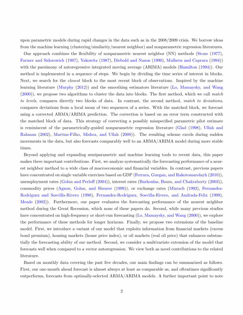
The Great Recession was a sobering experience in many dimensions. One such lesson came from the

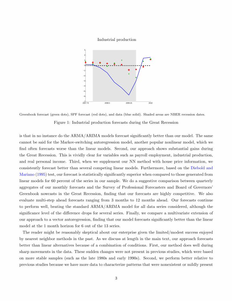
difficulties that macroeconometric models had in predicting the abrupt swings around the crisis. Figure

1 shows data for industrial production growth as well as one quarter ahead forecasts from the Survey of

Professional Forecasters and the Board of Governors’ Greenbook. It is not difficult to see that the forecasts

were off during the recession. Both the Greenbook and SPF forecasts called for much higher industrial

production growth through much of the crisis. Not surprisingly, macroeconomists were criticized for the poor

performance of their forecasts (Ferrara, Marcellino, and Mogliani (2015), Del Negro and Schorfheide (2013),

Potter (2011)). Given this grim backdrop, in this paper, we develop a forecasting algorithm that improves

∗Holt Dwyer provided excellent research assistance. We thank Todd Clark, Francis Diebold, Thorsten Drautzburg, LucaGuerrieri, Aaron Hall, Kirstin Hubrich, Ed Knotek, Mohammad Jahan-Parvar, Michael McCracken, Juan Rubio-Ramirez,Frank Schorfheide, Mototsugu Shintani, Minchul Shin, Ellis Tallman, Filip Zikes for valuable discussions. We also thankseminar participants at the Computational and Financial Econometrics 2016 meetings, Midwest Econometrics 2016, MidwestMacro 2016, the Federal Reserve Board, and the Federal Reserve Bank of Cleveland. This paper does not necessarily reflectthe views of the Federal Reserve System or its Board of Governors.†Boston College and ESPOL, pguerron@gmail.com‡Federal Reserve Board, molin.zhong@frb.gov

1

upon parametric models during rapid changes in the data such as in the 2008/2009 crisis. We borrow ideas

from the machine learning (clustering/similarity/nearest neighbor) and nonparametric regression literatures.

Our approach combines the flexibility of nonparametric nearest neighbor (NN) methods (Stone (1977),

Farmer and Sidorowich (1987), Yakowitz (1987), Diebold and Nason (1990), Mulhern and Caprara (1994))

with the parsimony of autoregressive integrated moving average (ARIMA) models (Hamilton (1994)). Our

method is implemented in a sequence of steps. We begin by dividing the time series of interest in blocks.

Next, we search for the closest block to the most recent block of observations. Inspired by the machine

learning literature (Murphy (2012)) and the smoothing estimators literature (Lo, Mamaysky, and Wang

(2000)), we propose two algorithms to cluster the data into blocks. The first method, which we call match

to levels, compares directly two blocks of data. In contrast, the second method, match to deviations,

compares deviations from a local mean of two sequences of a series. With the matched block, we forecast

using a corrected ARMA/ARIMA prediction. The correction is based on an error term constructed with

the matched block of data. This strategy of correcting a possibly misspecified parametric pilot estimate

is reminiscent of the parametrically-guided nonparametric regression literature (Glad (1998), Ullah and

Rahman (2002), Martins-Filho, Mishra, and Ullah (2008)). The resulting scheme excels during sudden

movements in the data, but also forecasts comparably well to an ARMA/ARIMA model during more stable

times.

Beyond applying and expanding semiparametric and machine learning tools to recent data, this paper

makes three important contributions. First, we analyze systematically the forecasting performance of a near-

est neighbor method to a wide class of macroeconomic and financial variables. In contrast, previous papers

have concentrated on single variable exercises based on GDP (Ferrara, Guegan, and Rakotomarolayh (2010)),

unemployment rates (Golan and Perloff (2004)), interest rates (Barkoulas, Baum, and Chakraborty (2003)),

commodity prices (Agnon, Golan, and Shearer (1999)), or exchange rates (Mizrach (1992), Fernandez-

Rodriguez and Sosvilla-Rivero (1998), Fernandez-Rodriguez, Sosvilla-Rivero, and Andrada-Felix (1999),

Meade (2002)). Furthermore, our paper evaluates the forecasting performance of the nearest neighbor

method during the Great Recession, which none of these papers do. Second, while many previous studies

have concentrated on high-frequency or short-run forecasting (Lo, Mamaysky, and Wang (2000)), we explore

the performance of these methods for longer horizons. Finally, we propose two extensions of the baseline

model. First, we introduce a variant of our model that exploits information from financial markets (excess

bond premium), housing markets (house price index), or oil markets (real oil price) that enhances substan-

tially the forecasting ability of our method. Second, we consider a multivariate extension of the model that

forecasts well when compared to a vector autoregression. We view both as novel contributions to the related

literature.

Based on monthly data covering the past five decades, our main findings can be summarized as follows.

First, our one-month ahead forecast is almost always at least as comparable as, and oftentimes significantly

outperforms, forecasts from optimally-selected ARMA/ARIMA models. A further important point to note

2

Industrial production

2007.75 2008.5 2009.25 2010−7

−6

−5

−4

−3

−2

−1

0

1

2

3

Greenbook forecast (green dots), SPF forecast (red dots), and data (blue solid). Shaded areas are NBER recession dates.

Figure 1: Industrial production forecasts during the Great Recession

is that in no instance do the ARMA/ARIMA models forecast significantly better than our model. The same

cannot be said for the Markov-switching autoregression model, another popular nonlinear model, which we

find often forecasts worse than the linear models. Second, our approach shows substantial gains during

the Great Recession. This is vividly clear for variables such as payroll employment, industrial production,

and real personal income. Third, when we supplement our NN method with house price information, we

consistently forecast better than several competing linear models. Furthermore, based on the Diebold and

Mariano (1995) test, our forecast is statistically significantly superior when compared to those generated from

linear models for 60 percent of the series in our sample. We do a suggestive comparison between quarterly

aggregates of our monthly forecasts and the Survey of Professional Forecasters and Board of Governors’

Greenbook nowcasts in the Great Recession, finding that our forecasts are highly competitive. We also

evaluate multi-step ahead forecasts ranging from 3 months to 12 months ahead. Our forecasts continue

to perform well, beating the standard ARMA/ARIMA model for all data series considered, although the

significance level of the difference drops for several series. Finally, we compare a multivariate extension of

our approach to a vector autoregression, finding that our model forecasts significantly better than the linear

model at the 1 month horizon for 6 out of the 13 series.

The reader might be reasonably skeptical about our enterprise given the limited/modest success enjoyed

by nearest neighbor methods in the past. As we discuss at length in the main text, our approach forecasts

better than linear alternatives because of a combination of conditions. First, our method does well during

sharp movements in the data. These sudden changes were not present in previous studies, which were based

on more stable samples (such as the late 1980s and early 1990s). Second, we perform better relative to

previous studies because we have more data to characterize patterns that were nonexistent or mildly present

3

in shorter samples. For example, we find that our approach uses information from the recessions in the 1970s

and 1980s to forecast industrial production and inflation during the Great Recession. These two points are

clearly seen in Figure 2, where we plot industrial production and inflation during the recent crisis (red lines)

and the best match from our approach (blue lines). The matched series indeed capture the sharp declines in

the variables of interest, which leads to a better forecast.1 Finally, our approach also needs that the series

under study be reasonably persistent. If the data lacks persistence or does not display consistent patterns

(as is the case with hourly earnings), our methodology does not improve over alternative linear approaches.

A further advantage of our estimation approach is its ease of computation and flexibility. Although in this

paper we only consider the canonical ARMA/ARIMA and VAR models as baselines, in theory any number

of linear or nonlinear models can be used as the baseline model in our framework. On top of the baseline

model, only two parameters of interest must be estimated: a match length parameter and a parameter that

governs the number of top matches over which to average. We choose these parameters based off of previous

out-of-sample forecasting performance using a mean squared error criterion.

(a) Industrial Production (b) Inflation

2007.5 2008 2008.5 2009 2009.5 2010

−4

−3

−2

−1

0

1

2007.5 2008 2008.5 2009 2009.5 2010−1.5

−1

−0.5

0

0.5

1

1.5

Red lines correspond to the actual data during the crisis. Blue lines correspond to the best matched series from our nearest

neighbor approach. Shaded areas are NBER recession dates.

Figure 2: Actual Data and Matched Series in the Great Recession

Our work is closely related to recent studies that emphasize the increasing difficulties in forecasting macroe-

conomic variables. For example, Stock and Watson (2007) conclude that inflation “has become harder to

forecast.” They advocate the use of time-varying parameters or stochastic volatility to capture the dynamics

of inflation. The Great Recession just reinforced the challenges that the profession faces when forecasting

the change in prices (Robert Hall, 2011 AER presidential address; Del Negro, Giannoni, and Schorfheide

(2014)). Our approach provides a fresh look into the inflation forecast conundrum. Importantly, similar

1We show in Section 5 that most of the matched series come from the 1980 recessions and a few observations from 1975.

4

to the findings of Del Negro, Giannoni, and Schorfheide (2014), we report that information from financial

markets (in particular, house prices) tends to improve forecasts during the Great Recession. Unlike Stock

and Watson (2007)’s and Del Negro, Hasegawa, and Schorfheide (2015)’s results, we find that using financial

information does not worsen the predictive power of our approach outside the crisis. Broadly speaking, we

view our methodology as a complementary tool to the collection of available methods to forecast macroeco-

nomic variables.

We proceed as follows. Sections 2 and 3 outline our methodology. We discuss the data and our forecasting

exercise in Section 4. We present an extension of our model that allows for exogenous data in Section 5.

The last section provides some final thoughts and conclusions.

2 Nearest Neighbor Matching Algorithm

We first briefly review the nearest neighbor econometric framework to fix ideas. Our forecasting model

builds on to this benchmark. Let YT = {y1, y2, . . . , yT } denote a collection of observations. We suppose a

general nonlinear autoregressive structure:

yt = g(yt−1, ...yt−k) + εt

with the assumption that E(εt|Yt−1) = 0.

The goal of the nearest neighbor algorithm is to estimate the conditional expectation function:

E(yt|Yt−1) = g(yt−1, ..., yt−k)

To this end, we form the following nonparametric estimator of the function g(yt−k, ..., yt−1):

g =

∑I(dist(yj−k:j−1, yt−k:t−1) ≤ distm(T )

)yj∑

I(dist(yj−k:j−1, yt−k:t−1) ≤ distm(T )

)where yt−k:t−1 = {yt−1, ..., yt−k}, I(.) is the indicator function, dist(., .) is a distance function to be defined

later, distm(T ) is a threshold level so that all matches with a distance below it are used. The summation

is over the number of matches. This number in turn depends on the sample size T . Allowing the number

of nearest neighbors m to grow slowly as the number of observations T increases (specifically, mT → 0

as m,T → ∞) is a crucial condition for consistency of the nearest neighbor estimator (Yakowitz (1987)).

Further detailed conditions on the convergence of the nearest neighbor estimator can be found in that paper,

an important one being a sufficient degree of smoothness of the g(.) function (at least twice continuously

differentiable).

Operationally, our objectives are 1) to cluster data in blocks of k elements, say Cj = {[yt1 , yt1+1, . . . , yt1+k−1],

[yt2 , yt2+1, . . . , yt2+k−1], . . . , [ytn , ytn+1, . . . , ytn+k−1]}; this cluster contains tn sets/blocks of observations of

5

size k each; and 2) assign the most recent k observations [yT−k+1, . . . , yT ] to some cluster with M denoting

the number of clusters; and 3) based on this assignment, forecast the next observation yT+1.

We propose two main classes of matching algorithms (distance functions):

1. Match to levels

2. Match to deviations from local mean

Matching to levels makes more sense either when the level of a data series itself has important economic

or forecasting value or when the series is clearly stationary. Matching to deviations from local mean makes

more sense when the researcher would like to match the directional movements of the series as opposed to

the overall level.

Match to levels The basic idea behind this alternative is to compare directly two sequences of series.

This takes into account both the overall level of the series and its movements.

Let us compare two sequences of series of length k (wlog to the first sequence of length k) [yt−k+1, . . . , yt]

vs. [y1, y2, . . . , yk]. The similarity between these two blocks of data is captured by the distance function:

dist =k∑i=1

weighs(i) (yt+1−i − yk+1−i)2 . (1)

Here, weighs(i) is the importance (or weight) given to observation i.

Match to deviations from local mean This alternative compares deviations from a local mean of two

sequences of a series. By doing so, we aim to capture the idea of matching directional movements of a series

rather than the overall levels.

As before, we are interested in comparing two sequences of series of length k : [yt−k+1, ..., yt] vs.

[y1, y2, ..., yk]. Denote yt as the local mean yt = 1k

∑kj=1 yt+1−j , then our similarity function is:

dist =

k∑i=1

weighs(i) ((yt+1−i − yt)− (yk+1−i − yk))2 .

In our empirical exercises, we choose weighs to be a decreasing, linear function in i.

weighs(i) =1

i

We think that this weighing function provides a good compromise between simplicity and giving the

6

highest weights to most recent observations.2 Upon fixing the weighting function, the empirical model is

completed by specifying the match length k and the number of forecasts to average over m.

3 Forecasting Model

Our approach is parsimonious. Relative to the baseline nearest neighbor algorithm, we adjust the current

forecast from a baseline ARMA/ARIMA model with the model’s forecast errors from previous similar

time periods, where similarity is defined by the distance function. This approach is in the same spirit

as the parametrically-guided nonparametric regression literature (Glad (1998), Ullah and Rahman (2002),

Martins-Filho, Mishra, and Ullah (2008)), which has shown the potential finite-sample benefits of using a

parametric pilot estimate to reduce the bias relative to a purely nonparametric regression without a variance

penalty.

Without loss of generality, let us suppose that the first sequence is the one that is matched, i.e. the

sequence that has the highest similarity (smallest distance) with the current sequence. To generate the

forecast, we use the following formula:

yt+1 = (yk+1 − yk+1,ARMA) + yt+1,ARMA,

where yt+1,ARMA is the forecast from an ARMA/ARIMA model. We select an ARMA/ARIMA model

as the auxiliary model because our data is monthly with high variability. Hence, an autoregressive model

would have a hard time capturing these movements.3,4

Of course, we must average the forecasts over the top m matches, which is what is done in the empirical

section. Formally, the adjusted forecasting model is

yt+1 =1

m

m∑ii

(yl(ii)+1 − yl(ii)+1,ARMA

)+ yt+1,ARMA

where {yl(ii)−k+1, yl(ii)−k+2, . . . , yl(ii)−1, yl(ii)} is the iith closest match to {yt−k+1, yt−k+2, . . . , yt−1, yt}.2Other weighing alternatives are Del Negro, Hasegawa, and Schorfheide (2015)’s dynamic weighs scheme and exponential

kernels as in Lo, Mamaysky, and Wang (2000).3A baseline nonparametric version of our approach would consist of using the next observation in the matched block as the

forecast. That is, suppose the first sequence gives the best match, then our forecast is yt+1 = yk+1. Alternatively, we could usea “random walk” forecast: yt+1 = yk

4To some degree, our approach is reminiscent of Frankel and Froot (1986)’s chartist-fundamentalist model of exchangerates. In their paper, a mixture of an ARIMA model (chartist) and Dornbusch’s overshooting (fundamentalist) model is usedto forecast exchange rates. If we take past patterns as proxies for fundamentals in the economy, we could argue that thefundamentalist component in our approach corresponds to the correction term yt+1,ARMA.

7

3.1 Discussion

Nearest neighbor methods have a decidedly local flavor, as emphasized by much of the previous literature

(e.g. Farmer and Sidorowich (1987), Diebold and Nason (1990)). This fact can be seen by noticing that

information contained in data related to the top m matches “close” to the current sequence at hand have full

weight in the adjustment step, whereas series “far” from this sequence have no weight5. This local nature

of the estimator is true for nonparametric estimation in general (Pagan and Ullah (1999)). We can contrast

this local behavior of the nearest neighbor estimator with global methods such as linear ARMA/ARIMA

models, which use all historical data with equal weight. The latter approach may be inappropriate during

times of crises, where economic relationships prevailing during normal times tend to break down6.

Furthermore, we believe that adjusting a preliminary forecast from an ARMA/ARIMA model is an im-

portant first step in the forecasting procedure. Monthly macroeconomic data is generally well-described by

ARMA or ARIMA dynamics, being a popular reduced-form model for consumption growth (Schorfheide,

Song, and Yaron (2014)) and unemployment (Montgomery, Zarnowitz, Tsay, and Tiao (1998)), among

many other macroeconomic series. The important moving average component often found when modeling

monthly data suggests the need to first remove these dynamics. Guiding the nonparametric estimator with

a parametric pilot has been proposed before on cross-sectional data, the general intuition being to choose

a parametric guide that is “close” to the true nonparametric function (Martins-Filho, Mishra, and Ullah

(2008)).

3.2 Recursive out-of-sample forecasting exercise

To perform out-of-sample forecasting, we have a few parameters that we would like to select to determine

the optimal forecasting model. We sketch an algorithm to select the match length k and how many forecasts

we average over m using predictive least squares.

Suppose we have KM forecasting models: all combinations of k = 1, 2, ...,K and m = 1, 2, ...,M . Index

the forecasts made by these models for time t with yt,km.

argmink,m1

t− t1

t∑τ=t1

(yτ − yτ,km)2 (2)

We select the optimal forecasting model by considering the out-of-sample forecasting performance as

evaluated by the mean squared error using data up until the current time period t (shown in the formula

above). We recursively select the optimal forecasting model at each time to forecast.7

5In the baseline nonparametric version of the approach, where we do not first estimate an ARMA/ARIMA model, sequencesfar from the current sequence have no bearing on the forecast.

6We thank Luca Guerrieri for raising our attention to this important point.7Our selection mechanism shares many similarities with bandwidth selection in kernel regressions. For an application in

8

An important issue is the choice of t1, which is the first time period of the model selection criterion. This

may be difficult to choose if the data have structural breaks , such as a break in the optimal lag length

value k∗. If so, a k∗,m∗ that does well at the beginning of the sample may not do well moving forward. We

could let t1 be rolling with t to account for structural breaks, although we do not do so in our empirical

application.

4 Illustrative simulation

Before we apply our methodology to the macroeconomic and financial data, we present an example of a

nonlinear data generating process in which our model performs well.

Our data generating process is the following:

yt = (1− Φ (a (mean (yt−10, .., yt−1)− a2))) (c+ φyt−1) +

Φ (a (mean (yt−10, .., yt−1)− a2)) (c2 + φ2yt−1) + σεt + θσεt−1(3)

where Φ is the normal cumulative distribution function. Importantly, this process implies a smooth function

of the past data so that Yakowitz (1987)’s conditions for consistency are met.

Table 1: Parameter Values

a 40 c2 0

a2 −0.043 φ2 0

c −0.002 σ 0.1

φ 0.95 θ −0.3

Table 1 shows the parameter values for the data generating process. The process falls in the class of smooth

transition autoregression (STAR) models. Intuitively, it transitions between two different regimes via a

nonlinear function of the data in the past 10 periods. The first regime has ”disaster”-type characteristics.

It has a lower intercept c. The data also becomes very persistent given the value of φ. The second regime is

a normal regime with no persistence. The parameter a2 controls the frequency of the first regime. We set

it so that the first regime occurs around 30% of the time. The parameter a controls how quickly transitions

occur from one regime to another.

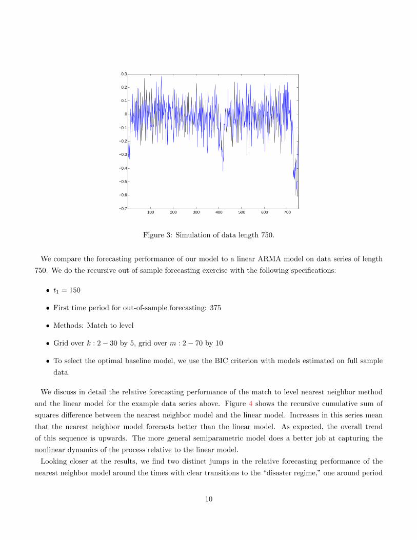
Figure 3 gives an example of a simulated series from the data generating process. Note that for most of the

time, regime 2 dominates. Occasionally, as can be seen around periods 400 and 700, a string of bad shocks

can trigger the model to enter into regime 1 dynamics. Importantly, as these transitions are functions of

past data, they are in theory predictable, although in a nonlinear fashion.

finance, see Lo, Mamaysky, and Wang (2000)

9

100 200 300 400 500 600 700−0.7

−0.6

−0.5

−0.4

−0.3

−0.2

−0.1

0

0.1

0.2

0.3

Figure 3: Simulation of data length 750.

We compare the forecasting performance of our model to a linear ARMA model on data series of length

750. We do the recursive out-of-sample forecasting exercise with the following specifications:

• t1 = 150

• First time period for out-of-sample forecasting: 375

• Methods: Match to level

• Grid over k : 2− 30 by 5, grid over m : 2− 70 by 10

• To select the optimal baseline model, we use the BIC criterion with models estimated on full sample

data.

We discuss in detail the relative forecasting performance of the match to level nearest neighbor method

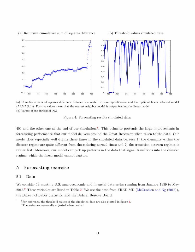
and the linear model for the example data series above. Figure 4 shows the recursive cumulative sum of

squares difference between the nearest neighbor model and the linear model. Increases in this series mean

that the nearest neighbor model forecasts better than the linear model. As expected, the overall trend

of this sequence is upwards. The more general semiparametric model does a better job at capturing the

nonlinear dynamics of the process relative to the linear model.

Looking closer at the results, we find two distinct jumps in the relative forecasting performance of the

nearest neighbor model around the times with clear transitions to the “disaster regime,” one around period

10

(a) Recursive cumulative sum of squares difference (b) Threshold values simulated data

400 450 500 550 600 650 700 750−0.1

0

0.1

0.2

0.3

0.4

0.5

0.6

0.7

400 450 500 550 600 650 700 7500

0.1

0.2

0.3

0.4

0.5

0.6

0.7

0.8

0.9

1

(a) Cumulative sum of squares difference between the match to level specification and the optimal linear selected model

(ARMA(1,1)). Positive values mean that the nearest neighbor model is outperforming the linear model.

(b) Values of the threshold Φ(.)

Figure 4: Forecasting results simulated data

400 and the other one at the end of our simulation.8. This behavior portends the large improvements in

forecasting performance that our model delivers around the Great Recession when taken to the data. Our

model does especially well during these times in the simulated data because 1) the dynamics within the

disaster regime are quite different from those during normal times and 2) the transition between regimes is

rather fast. Moreover, our model can pick up patterns in the data that signal transitions into the disaster

regime, which the linear model cannot capture.

5 Forecasting exercise

5.1 Data

We consider 13 monthly U.S. macroeconomic and financial data series running from January 1959 to May

2015.9 These variables are listed in Table 2. We use the data from FRED-MD (McCracken and Ng (2015)),

the Bureau of Labor Statistics, and the Federal Reserve Board.

8For reference, the threshold values of the simulated data are also plotted in figure 4.9The series are seasonally adjusted when needed.

11

5.2 Details

We do the recursive out-of-sample forecasting exercise for the data series in our sample with the following

specifications:

• t1 = Jan 1975

• First time period for out-of-sample forecasting: Jan 1990

• Methods: Match to level, match to deviations from local mean

• Grid over k : 2− 70 by 10, grid over m : 2− 80 by 10

• To select the optimal baseline model, we do the following. First, we perform augmented Dickey-Fuller

tests of stationarity for the series. For the series in which we cannot reject the null of a unit root, we

compare the BIC values of the BIC-selected ARMA model with the BIC-selected ARIMA model. For

series in which we do reject the null of stationarity, we select the best ARMA model using BIC. Note

that for this model-selection step only, we use full sample data.

5.3 Results

The column labeled NN1 in Table 2 compares the forecast from our match to level specification model versus

the forecast from an optimally selected ARMA/ARIMA model. A quick look at the table reveals that our

approach does better (Y ) than the alternative for all variables but the federal funds rate, unemployment,

and hourly earnings.10 At the 5% level using the Diebold-Mariano test, the match to level specification

forecasts better for inflation, industrial production, real personal income, and commercial and industrial

loans. In addition, the match to level specification forecasts better than the linear model at the 10% level

for payroll employment. When we switch to the match to deviations specification (column NN2), our model

performs better than the linear alternative for all data series. The forecast is superior at the 5% level for

unemployment, IP, real personal income, and real estate loans. It forecasts better at the 10% level for

personal consumption expenditures.

10Relative RMSE values are in the appendix. 12

Table 2: Forecast comparison based on MSE (1 step ahead)

ρ σ NN1 NN2 MS-AR NNX-B NNX-H NNX-O ARMAX-B ARMAX-H ARMAX-O

Inflation 0.72 0.27 Y ∗∗ Y N Y ∗ Y ∗∗ Y ∗∗ N Y Y ∗∗

Federal funds rate 0.99 4.00 N Y − Y Y N N Y Y

Unemployment 0.99 1.57 N Y ∗∗ N Y ∗ Y ∗∗ Y Y Y N

Payroll employment 0.7 217.1 Y ∗ Y Y (N)† Y Y ∗ Y Y N N

Industrial production 0.35 0.73 Y ∗∗ Y ∗∗ Y Y Y ∗ Y Y N N

Personal consumption -0.22 0.51 Y Y ∗ N Y Y ∗ Y N N N

Real personal income -0.14 0.61 Y ∗∗ Y ∗∗ N Y Y ∗∗ Y ∗ Y Y Y

Average hourly earnings 0.02 0.29 N Y N Y ∗∗ Y Y ∗∗ Y N Y ∗

Housing starts -0.31 8.18 Y Y Y Y ∗ Y ∗∗ Y N N N

Capacity utilization 0.99 4.65 Y Y Y ∗∗ Y Y Y Y N N

S&P500 0.25 3.56 Y Y N Y N Y Y N N

Real estate loans 0.65 0.64 Y Y ∗∗ Y Y ∗∗ Y ∗∗ Y ∗∗ N Y N

Commercial and industrial loans 0.73 0.89 Y ∗∗ Y Y ∗∗ Y ∗∗ Y Y Y ∗∗ N N

Note: Comparisons relative to ARMA/ARIMA model. NN1: match to level model; NN2: match to deviation model. “Y ” means that our proposed

model does better than the alternative. Based on the Diebold-Mariano test, an asterisk (∗) and a double asterisk (∗∗) mean that the forecast is better

at 10 % and 5 %, respectively. We use Newey-West standard errors when making these calculations.

ρ and σ correspond to the autocorrelation and standard deviation.

Note that while the comparisons NN1 and NN2 are made for models estimated on the data from 1959 until the end of the sample, the other comparisons

are made for models estimated beginning in 1973 due to data limitation issues.

The MS-AR model is not estimated for the Federal funds rate because of convergence problems.

†: The MS-AR model has difficulty estimating recursively for payroll employment. The model is able to estimate using the entire sample as well as using

data only up to Jan 1990 (the first time period for the forecasting exercise). Forecasting using full sample parameter estimates leads to better performance

versus the linear model whereas forecasting using parameter estimates with information up to Jan 1990 leads to poorer forecasting performance.

13

The relative success of our method rests on a combinations of elements. First, the data under study need to

be persistent and display patterns. Without these features, there is no valuable information in past data to

be exploited. Second, we need several episodes of sudden movements, such as during recessions. This means

that our approach benefits from longer history of data. To shed light on these issues, we discuss in some

detail the results for 3 important macro series: payroll employment, industrial production, and personal

consumption expenditures and one financial series: commercial and industrial loans. We find many large

forecasting gains during the Great Recession time period for each of these series discussed. Indeed, for

almost all of the series that exhibit significant forecasting gains, we find large improvements during the

Great Recession. We also discuss the forecast of hourly earnings as a case in which our method does not

improve over linear models. As will become clear momentarily, this failure results from the lack of historical

patterns (especially around recessions) in the hourly earnings series.

Payroll employment Nonfarm payroll employment is the change in the number of paid workers from

the previous month excluding general governmental, private household, nonprofit, and farm employees.

From panel (a) in Figure 5, we see that the data is mildly persistent, with a first-order autocorrelation

of around 0.6. Entering recessions, payroll employment sharply declines whereas recoveries feature more

gradual increases in the data series. The past 3 recessions have seen pronounced slow payroll employment

rebounds. Especially notable is the decline during the recent Great Recession, which is by far the largest

decline in the data sample.

In forecasting the recent time period, we look at past similar historical patterns. Crucial for our purposes,

Figure 5 shows a sharp contraction in payroll employment during the 1974 recession, with employment

declining by 604, 000 between October and December of that year. In terms of persistence, the 1982 episode

provides some valuable information regarding the lingering effects of recessions on employment. It took

roughly 18 months for payroll employment to return to positive growth. This number provides a reasonable

proxy for the 2 years needed during the Great Recession

Panel (b) in Figure 5 shows the recursive cumulative sum of squares difference between the nearest neighbor

method using match to level and the optimally selected linear model, which is an ARMA(2,1). Positive

values mean that the nearest neighbor model is forecasting better than the linear model. The proposed

methodology does especially well during recession dates, with the largest jump occurring during the Great

Recession. The methodology also does especially well in the late 1990’s, but otherwise the two methods

appear to perform quite similarly in expansionary times.

The particularly large gain in forecasting performance motivates us to examine the Great Recession period

in more depth. Panel (d) in Figure 5 presents the movements of payroll employment and the resulting linear

(blue) and nearest neighbor (red) forecast errors across the Great Recession. Payroll employment change

tanks in the Great Recession, reaching around −900, 000 in late 2008 and early 2009. These declines are

difficult for the linear model to forecast, as evidenced by the consistently positive forecast errors through-

14

(a) Monthly nonfarm payroll employment (thousands) (b) Recursive cumulative sum of squares difference†

1960 1970 1980 1990 2000 2010−1000

−500

0

500

1000

1500

1995 2000 2005 2010 2015−1

0

1

2

3

4

5x 105

(c) Payroll in Great Recession (thousands) (d) Forecast errors‡

2007.5 2008 2008.5 2009 2009.5 2010−1000

−500

0

500

2007.5 2008 2008.5 2009 2009.5 2010−400

−300

−200

−100

0

100

200

300

400

500

600

†Cumulative sum of squares difference between the match to level specification and the optimal linear selected model

(ARMA(2,1)). Positive values mean that the nearest neighbor model is outperforming the linear model.‡Forecast errors (Blue - linear model and Red - nearest neighbor model). Shaded areas are NBER recession dates.

Figure 5: Payroll Employment

15

out the recession. While the nearest neighbor method also generates too optimistic forecasts, its forecast

errors are below those of the linear model during the Great Recession. The nearest neighbor method does

especially well predicting the large decrease in payroll employment change beginning in the middle of 2008.

Interestingly, our method outperforms the linear model even after the Great Recession (note the smaller

forecast errors in panel (d)). However, this is not a general finding, as we will see momentarily.

(a) Growth rate (percent) (b) Recursive cumulative sum of squares difference†

1960 1970 1980 1990 2000 2010−6

−4

−2

0

2

4

6

1995 2000 2005 2010 2015−4

−2

0

2

4

6

8

10

12

(c) IP in Great Recession (percent) (d) Forecast errors‡

2007.5 2008 2008.5 2009 2009.5 2010−5

−4

−3

−2

−1

0

1

2

2007.5 2008 2008.5 2009 2009.5 2010−3

−2

−1

0

1

2

3

4

5

†Cumulative sum of squares difference between the match to level specification and the optimal linear selected model

(ARMA(4,2)). Positive values mean that the nearest neighbor model is outperforming the linear model.‡Forecast errors (Blue - linear model and Red - nearest neighbor model). Shaded areas are NBER recession dates.

Figure 6: Industrial Production

16

Industrial production Industrial production growth is the monthly growth rate of the Federal Reserve

Board’s index of industrial production. This index covers manufacturing, mining, and electric and gas utili-

ties. Industrial production (panel (a) in Figure 6) is much less persistent than nonfarm payroll employment

changes, with a first order autocorrelation of around 0.4. Like nonfarm payroll employment, it is highly

procyclical, declining during recessions. The Great Recession had declines of industrial production of over

−4% per month (panel (c) in Figure 6), which was the deepest decline of any recession in the data sample.

Industrial production also declined drastically during the recession in the mid−1970s.

Panel (b) in Figure 6 compares the forecasting performance of the nearest neighbor match to level speci-

fication to the linear model, which is an ARMA(4,2). The nearest neighbor specification begins to do well

in 1995. Contrary to the payroll employment results, the nearest neighbor model appears to consistently

outperform the linear model at approximately the same rate from 1995 to the eve of the Great Recession.

The nonlinear method does especially well in the Great Recession and the two methods are comparable

afterwards.

As panel (d) in Figure 6 shows, the nearest neighbor method does especially well in the initial periods of the

Great Recession. The linear model overpredicts industrial production growth throughout the early part of

2008, while the nearest neighbor model has smaller positive forecast errors. It also has slight improvements

relative to the linear model in forecasting the second large dip in late 2008.

Personal consumption expenditures In contrast to the other data series, PCE growth is slightly

negatively autocorrelated at the monthly level (panel (a) in Figure 7). PCE growth declines in recessions,

although overall the data is quite noisy. While the Great Recession did not have any especially large

decreases in PCE growth, a notable feature is the particularly extended period of negative growth.

Panel (a) in Figure 7 compares the forecasting performance of the linear model (ARMA(1,2)) to that of the

nearest neighbor method using the deviations from local mean specification. The nearest neighbor method

does especially well at the end of the recession in the early 1990s and during the Great Recession. During

periods of expansion and in the early 2000s recession, there is not too large of a forecasting difference. The

nearest neighbor model also continues to forecast well after the Great Recession.

As can be seen by looking at the forecast errors in panel (d) in Figure 7, both the linear and nearest

neighbor models consistently overpredict future consumption growth throughout the Great Recession. The

nearest neighbor specification has the largest forecasting gains in the steep consumption growth declines in

mid-2008. It also does especially well at predicting the gradual rise in consumption growth at the end of

the recession. Finally, panel (d) also reveals that as the economy moved out of the recession, forecasts using

our approach are comparable to those from the linear specification.

Average hourly earnings As Figure 8 shows, our approach can also underperform relative to the linear

model. This is the case for real average hourly earnings growth. Across our sample period, average hourly

17

(a) Growth rate (percent) (b) Recursive cumulative sum of squares difference†

1960 1970 1980 1990 2000 2010−3

−2

−1

0

1

2

3

1995 2000 2005 2010 2015−1

−0.5

0

0.5

1

1.5

2

(c) PCE in Great Recession (percent) (d) Forecast errors‡

2007.5 2008 2008.5 2009 2009.5 2010−1.5

−1

−0.5

0

0.5

1

1.5

2007.5 2008 2008.5 2009 2009.5 2010−1.5

−1

−0.5

0

0.5

1

1.5

†Cumulative sum of squares difference between the match to deviations from local mean specification and the optimal linear

selected model (ARMA(1,2)). Positive values mean that the nearest neighbor model is outperforming the linear model.‡Forecast errors (Blue - linear model and Red - nearest neighbor model). Shaded areas are NBER recession dates.

Figure 7: Personal Consumption Expenditures

18

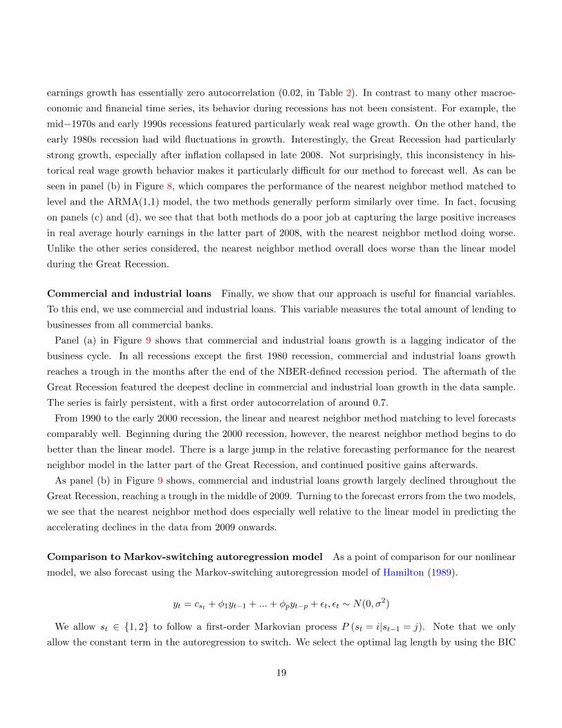
earnings growth has essentially zero autocorrelation (0.02, in Table 2). In contrast to many other macroe-

conomic and financial time series, its behavior during recessions has not been consistent. For example, the

mid−1970s and early 1990s recessions featured particularly weak real wage growth. On the other hand, the

early 1980s recession had wild fluctuations in growth. Interestingly, the Great Recession had particularly

strong growth, especially after inflation collapsed in late 2008. Not surprisingly, this inconsistency in his-

torical real wage growth behavior makes it particularly difficult for our method to forecast well. As can be

seen in panel (b) in Figure 8, which compares the performance of the nearest neighbor method matched to

level and the ARMA(1,1) model, the two methods generally perform similarly over time. In fact, focusing

on panels (c) and (d), we see that that both methods do a poor job at capturing the large positive increases

in real average hourly earnings in the latter part of 2008, with the nearest neighbor method doing worse.

Unlike the other series considered, the nearest neighbor method overall does worse than the linear model

during the Great Recession.

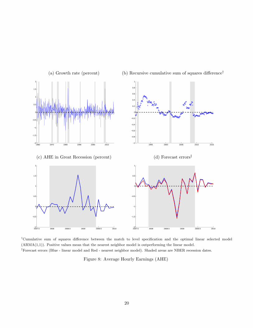
Commercial and industrial loans Finally, we show that our approach is useful for financial variables.

To this end, we use commercial and industrial loans. This variable measures the total amount of lending to

businesses from all commercial banks.

Panel (a) in Figure 9 shows that commercial and industrial loans growth is a lagging indicator of the

business cycle. In all recessions except the first 1980 recession, commercial and industrial loans growth

reaches a trough in the months after the end of the NBER-defined recession period. The aftermath of the

Great Recession featured the deepest decline in commercial and industrial loan growth in the data sample.

The series is fairly persistent, with a first order autocorrelation of around 0.7.

From 1990 to the early 2000 recession, the linear and nearest neighbor method matching to level forecasts

comparably well. Beginning during the 2000 recession, however, the nearest neighbor method begins to do

better than the linear model. There is a large jump in the relative forecasting performance for the nearest

neighbor model in the latter part of the Great Recession, and continued positive gains afterwards.

As panel (b) in Figure 9 shows, commercial and industrial loans growth largely declined throughout the

Great Recession, reaching a trough in the middle of 2009. Turning to the forecast errors from the two models,

we see that the nearest neighbor method does especially well relative to the linear model in predicting the

accelerating declines in the data from 2009 onwards.

Comparison to Markov-switching autoregression model As a point of comparison for our nonlinear

model, we also forecast using the Markov-switching autoregression model of Hamilton (1989).

yt = cst + φ1yt−1 + ...+ φpyt−p + εt, εt ∼ N(0, σ2)

We allow st ∈ {1, 2} to follow a first-order Markovian process P (st = i|st−1 = j). Note that we only

allow the constant term in the autoregression to switch. We select the optimal lag length by using the BIC

19

(a) Growth rate (percent) (b) Recursive cumulative sum of squares difference†

1960 1970 1980 1990 2000 2010−2

−1.5

−1

−0.5

0

0.5

1

1.5

2

1995 2000 2005 2010 2015−1

−0.8

−0.6

−0.4

−0.2

0

0.2

0.4

0.6

0.8

1

(c) AHE in Great Recession (percent) (d) Forecast errors‡

2007.5 2008 2008.5 2009 2009.5 2010−1

−0.5

0

0.5

1

1.5

2

2007.5 2008 2008.5 2009 2009.5 2010−2

−1.5

−1

−0.5

0

0.5

1

†Cumulative sum of squares difference between the match to level specification and the optimal linear selected model

(ARMA(1,1)). Positive values mean that the nearest neighbor model is outperforming the linear model.‡Forecast errors (Blue - linear model and Red - nearest neighbor model). Shaded areas are NBER recession dates.

Figure 8: Average Hourly Earnings (AHE)

20

(a) Growth rate (percent) (b) Recursive cumulative sum of squares difference†

1960 1970 1980 1990 2000 2010−3

−2

−1

0

1

2

3

4

1995 2000 2005 2010 2015−1

0

1

2

3

4

5

(c) C&I Loans in Great Recession (percent) (d) Forecast errors‡

2007.5 2008 2008.5 2009 2009.5 2010−3

−2

−1

0

1

2

3

4

2007.5 2008 2008.5 2009 2009.5 2010−3

−2

−1

0

1

2

3

4

†Cumulative sum of squares difference between the match to level specification and the optimal linear selected model

(ARMA(1,1)). Positive values mean that the nearest neighbor model is outperforming the linear model.‡Forecast errors (Blue - linear model and Red - nearest neighbor model). Shaded areas are NBER recession dates.

Figure 9: Commercial and industrial loans

21

criterion on an autoregressive model without Markov-switching. After selecting the autoregressive model, we

add Markov-switching to the intercept, allowing for two states. The Markov-switching models are estimated

using maximum likelihood.

We perform a recursive out-of-sample forecasting exercise and the results are shown in the column under

MS-AR in Table 2. In contrast to the nearest neighbor methods, which forecast better than the linear model

for most series, the Markov-switching model oftentimes forecasts worse. Of the six series in which Markov-

switching model forecasts worse when compared to the linear model, the forecasting difference is significant

for unemployment and personal consumption expenditures. In contrast, the linear model does not forecast

significantly better than the nearest neighbor model for any of the series considered. The Markov-switching

model does forecast significantly better than the linear model for capacity utilization and commercial and

industrial loans.

6 Can we do better?

The results so far indicate that our approach does particularly well during the Great Recession. Researchers

and policymakers alike have begun to develop theories on the drivers of the recent downturn - two of

which are based on the financial sector and housing disturbances. Moreover, oil price fluctuations have also

traditionally been an intriguing explanation of recessions. To exploit this potentially important information,

in this section, we present a methodology to incorporate financial, housing, and oil price data into our baseline

forecasting model.

To most economic commentators, the financial sector played a crucial role during the 2008/2009 crisis.

For instance, Gilchrist and Zakrajsek (2012) argue that credit spreads “contain important signals regarding

the evolution of the real economy and risks to the economic outlook.” By the same token, the boom/bust

cycle in the housing market was another key player before, during, and after the Great Recession (Farmer

(2012)). Moreover, theoretical studies on the relationship between financial frictions and housing and the

macroeconomy suggest that each could have a potentially important nonlinear relationship with general

macroeconomic performance (Mendoza (2010); Guerrieri and Iacoviello (2013)). Likewise, recessions are

also often preceded by a run-up in oil prices. For some economic observers, these sudden movements in oil

prices are, at least to some degree, responsible for the subsequent crises (Hamilton (2009)). Hence, it seems

natural to exploit these sources of information in our methodology.

To this end, we modify our algorithm as follows. Let xt denote a potential driver of the Great Recession

(credit spreads, housing prices, or oil prices). As before, we compare deviations from a local mean of two

sequences of the driver xt of length k [xt−k+1, ..., xt] vs. [x1, x2, ..., xk] based on the similarity function:

dist =k∑i=1

weighs(i) ((xt+1−i − xt)− (xk+1−i − xk))2 .

22

For simplicity, suppose that the first sequence is the one that is matched. Then our modified model, which

we call Nearest neighbor X is

yt+1 = (yk+1 − yk+1,ARMA)︸ ︷︷ ︸Error from matched time period

+ yt+1,ARMA,

We proceed in a similar fashion as with our benchmark model - specifically by conducting a recursive out-

of-sample forecasting exercise. We use similar grid points over k and m.11 An important point to note is that

because our objective function continues to be equation 2, which changes in accordance with the changing

variables to be forecast, it is possible to have different sequences of estimated k and m across the yt series,

even when using the same xt variable. For comparison purposes, we also forecast using ARMA/ARIMA

and ARMAX/ARIMAX models.

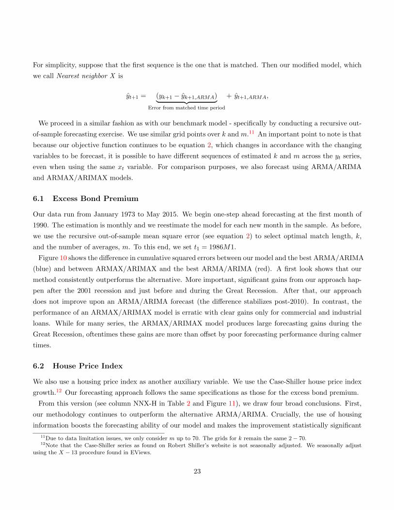
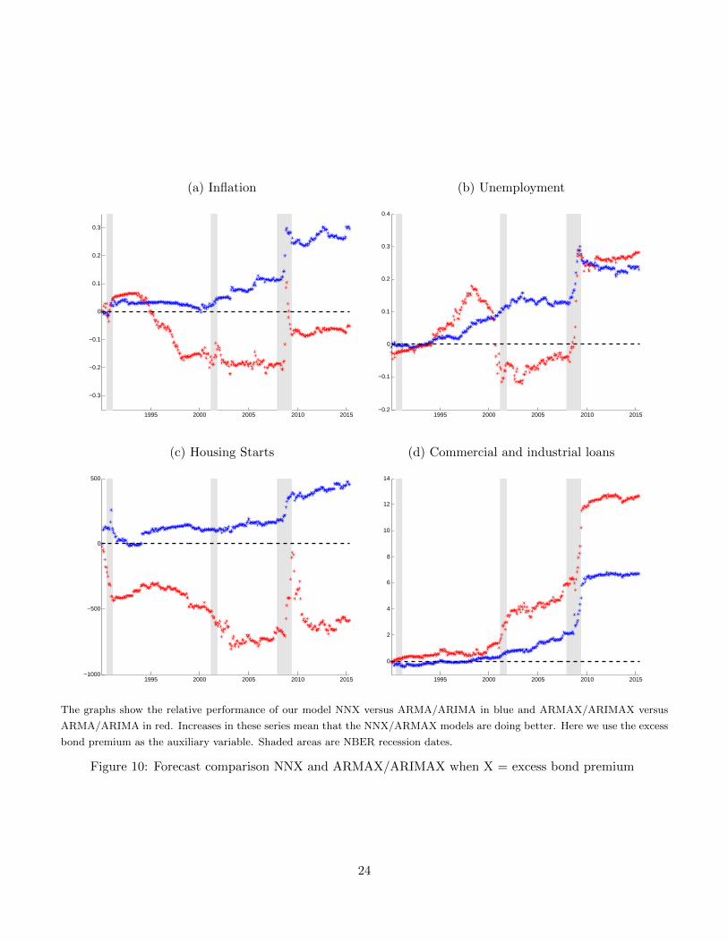
6.1 Excess Bond Premium

Our data run from January 1973 to May 2015. We begin one-step ahead forecasting at the first month of

1990. The estimation is monthly and we reestimate the model for each new month in the sample. As before,

we use the recursive out-of-sample mean square error (see equation 2) to select optimal match length, k,

and the number of averages, m. To this end, we set t1 = 1986M1.

Figure 10 shows the difference in cumulative squared errors between our model and the best ARMA/ARIMA

(blue) and between ARMAX/ARIMAX and the best ARMA/ARIMA (red). A first look shows that our

method consistently outperforms the alternative. More important, significant gains from our approach hap-

pen after the 2001 recession and just before and during the Great Recession. After that, our approach

does not improve upon an ARMA/ARIMA forecast (the difference stabilizes post-2010). In contrast, the

performance of an ARMAX/ARIMAX model is erratic with clear gains only for commercial and industrial

loans. While for many series, the ARMAX/ARIMAX model produces large forecasting gains during the

Great Recession, oftentimes these gains are more than offset by poor forecasting performance during calmer

times.

6.2 House Price Index

We also use a housing price index as another auxiliary variable. We use the Case-Shiller house price index

growth.12 Our forecasting approach follows the same specifications as those for the excess bond premium.

From this version (see column NNX-H in Table 2 and Figure 11), we draw four broad conclusions. First,

our methodology continues to outperform the alternative ARMA/ARIMA. Crucially, the use of housing

information boosts the forecasting ability of our model and makes the improvement statistically significant

11Due to data limitation issues, we only consider m up to 70. The grids for k remain the same 2− 70.12Note that the Case-Shiller series as found on Robert Shiller’s website is not seasonally adjusted. We seasonally adjust

using the X − 13 procedure found in EViews.

23

(a) Inflation (b) Unemployment

1995 2000 2005 2010 2015

−0.3

−0.2

−0.1

0

0.1

0.2

0.3

1995 2000 2005 2010 2015−0.2

−0.1

0

0.1

0.2

0.3

0.4

(c) Housing Starts (d) Commercial and industrial loans

1995 2000 2005 2010 2015−1000

−500

0

500

1995 2000 2005 2010 2015

0

2

4

6

8

10

12

14

The graphs show the relative performance of our model NNX versus ARMA/ARIMA in blue and ARMAX/ARIMAX versus

ARMA/ARIMA in red. Increases in these series mean that the NNX/ARMAX models are doing better. Here we use the excess

bond premium as the auxiliary variable. Shaded areas are NBER recession dates.

Figure 10: Forecast comparison NNX and ARMAX/ARIMAX when X = excess bond premium

24

for 8 out of 13 variables. Second, the forecasting performance improves dramatically for housing starts,

unemployment, and real state loans (see Figure 11) during the entire forecasting window (1990 - 2015).

Third, our approach improves even for those variables that display weak or no autocorrelation (personal

consumption and average hourly earnings). Finally, housing information also helps forecasting for some

series based on an ARMAX/ARIMAX model (last column in Table 2). However, the improvement is not

statistically significant as it only gives a boost to the forecast during a small part of the sample.

Figure 12 shows the time period of the last observation for the best matched block around the Great

Recession for some variables. In our notation (see equation 1), the (x, y) coordinates correspond to yt and

yk, respectively. For inflation (panel a), we observe that forecasting during most of the 2008/2009 crisis drew

heavily on the relationship between house prices and inflation during the 1980s. Our approach also grabs

some information from the 1970s. This is hardly surprising given the sharp comovements that inflation and

house prices experienced during the 1975 and 1980-1982 recessions. As we move out of the crisis, we rely

on more recent information to forecast inflation. The story behind industrial production (panel d) is a bit

similar to that behind inflation. To forecast during the early part of the Great Recession, our approach

relies on information from the 1980s. During the early part of 2009, our approach picks information from

2008 to generate the best matched block.

The unemployment (panel b) and payroll employment (panel c) series offer some important insights about

our method. The best match, yk, and the last observation, yt, display an almost linear relation around the

crisis. For example, the best matches for January 2008 and January 2010 are December 2007 and December

2009, respectively. That is, our approach is choosing recent information about the labor market as the most

relevant to forecast in 2008/2009. Does this mean that the past history is irrelevant? The answer is no. To

see this point, the red circles and black stars display the second and third matches picked by our method.

The reader now can see that the recessions from the 1980s and 1990s provided some useful information to

forecast unemployment early in the Great Recession. Yet the dire increase in unemployment at the trough

of the crisis forces our method to look at the more recent available data. It is also clear that as the economy

starts to heal, information from previous recoveries are handy. The payroll employment series tells us a

very similar story, albeit with some small twists. For completeness, we also provide the matched series for

housing starts (panel e) and commercial and industrial loans (panel f).

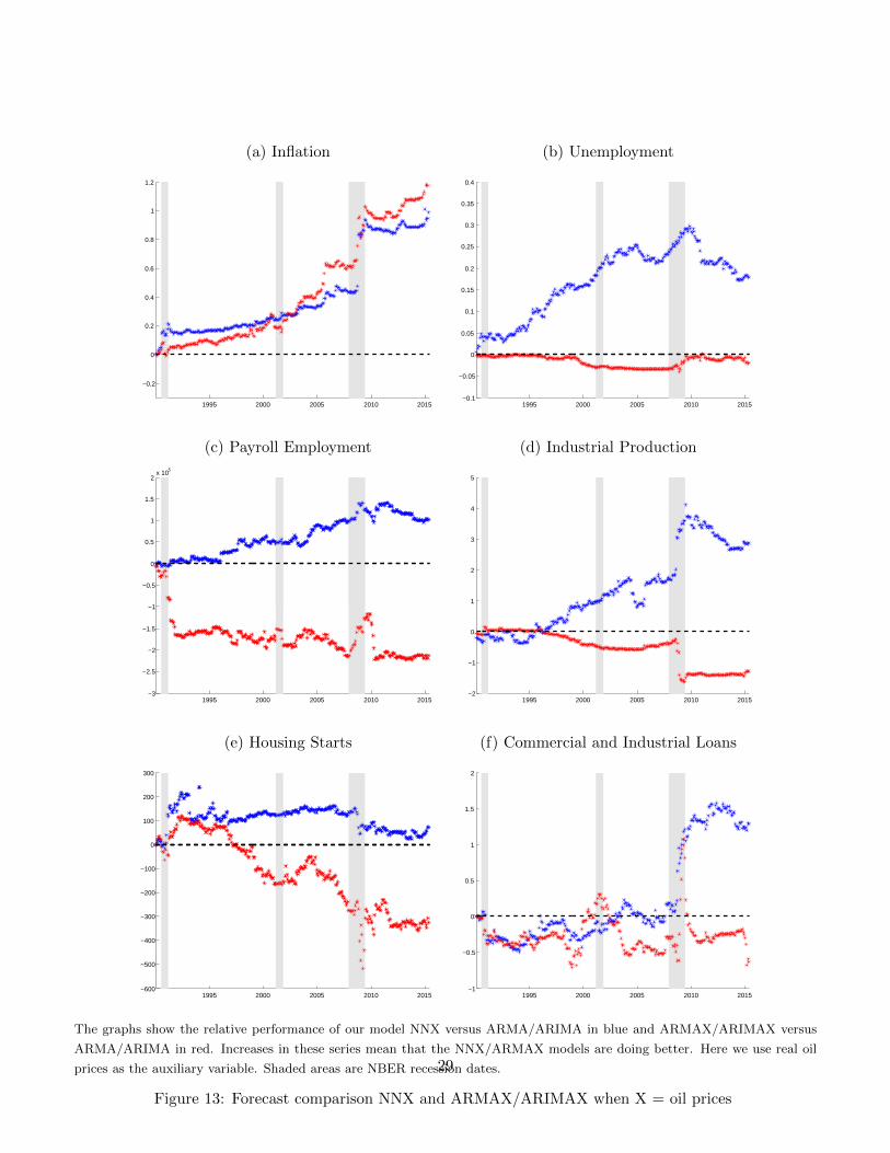
6.3 Real oil price

We also try oil prices as the auxiliary variable in our nearest neighbor method (see Table 2 and Figure 13).

Overall, the NNX-O variant forecasts all series well relative to the ARMA/ARIMA model with the excep-

tion of the fed funds rate. While the NNX-O model oftentimes does better relative to the ARMA/ARIMA

benchmark, the differences are significant for only inflation, average hourly earnings, and real estate loans.

The ARMAX/ARIMAX model has similarly strong forecasting performance for inflation and average hourly

earnings. It does poorly for real estate loans. On the other hand, we find that adding in oil price informa-

25

(a) Inflation (b) Unemployment

1995 2000 2005 2010 2015

−0.2

0

0.2

0.4

0.6

0.8

1

1995 2000 2005 2010 2015

−0.2

−0.1

0

0.1

0.2

0.3

0.4

0.5

(c) Payroll Employment (d) Industrial Production

1995 2000 2005 2010 2015−0.5

0

0.5

1

1.5

2

2.5

3

3.5

4

4.5

5

1995 2000 2005 2010 2015−2

−1

0

1

2

3

4

5

6

7

8

9

(e) Housing Starts (f) Commercial and Industrial Loans

1995 2000 2005 2010 2015

−600

−400

−200

0

200

400

600

1995 2000 2005 2010 2015−3

−2

−1

0

1

2

3

The graphs show the relative performance of our model NNX versus ARMA/ARIMA in blue and ARMAX/ARIMAX versus

ARMA/ARIMA in red. Increases in these series mean that the NNX/ARMAX models are doing better. Here we use house

prices as the auxiliary variable. Shaded areas are NBER recession dates.

Figure 11: Forecast comparison NNX and ARMAX/ARIMAX when X = house prices

26

(a) Inflation (b) Unemployment

2007.5 2008 2008.5 2009 2009.5 2010

1975

1980

1985

1990

1995

2000

2005

2010

2007.5 2008 2008.5 2009 2009.5 2010

1975

1980

1985

1990

1995

2000

2005

2010

(c) Payroll Employment (d) Industrial Production

2007.5 2008 2008.5 2009 2009.5 2010

1975

1980

1985

1990

1995

2000

2005

2010

2007.5 2008 2008.5 2009 2009.5 2010

1975

1980

1985

1990

1995

2000

2005

2010

(e) Housing Starts (f) Real Estate Loans

2007.5 2008 2008.5 2009 2009.5 2010

1975

1980

1985

1990

1995

2000

2005

2010

2007.5 2008 2008.5 2009 2009.5 2010

1975

1980

1985

1990

1995

2000

2005

2010

The graphs show the matched periods during the Great Recession when we use the NNX model and house prices as the auxiliary

variable. The blue line gives the corresponding best matched time period, the red circles give the second best, and the black

stars give the third best. Shaded areas are NBER recession dates.

Figure 12: Matched periods during Great Recession when X = house prices

27

tion linearly oftentimes hurts forecasting performance relative to the ARMA/ARIMA benchmark. From a

forecasting perspective, we find weaker evidence of a nonlinear relationship between oil price fluctuations

and the macroeconomy compared to the other explanatory variables.

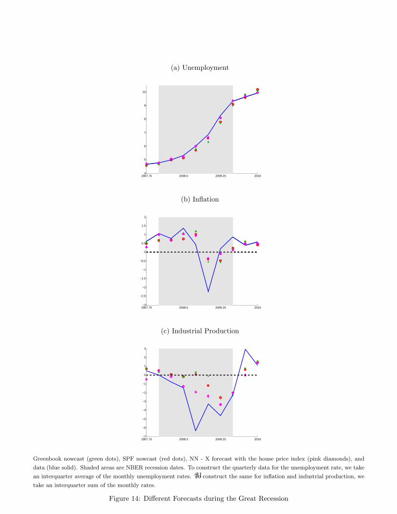
6.4 Comparison to survey-based nowcasts

Motivated by the forecasting performance of our NN-X method that uses house prices as an explanatory

variable, we find it illustrative to compare the method with alternative forecasts. Figure 14 shows the

Greenbook nowcasts (green dots), the SPF nowcasts (red dots), our approach using house prices as an

explanatory variable (pink diamonds), and the data (blue line) for unemployment, inflation, and industrial

production. As we are time-aggregating one-period ahead monthly forecasts to form quarterly forecasts

with our method, we use survey-based nowcasts in an effort to keep the information sets approximately the

same. Overall, we do better than the Greenbook forecasts for unemployment and industrial production.

The Greenbook survey tends to underpredict unemployment and overpredict industrial production growth.

We do better than the SPF forecast for industrial production growth and are competitive for the other

two data series. We do better in predicting the large drop in industrial production growth and increase in

unemployment during the middle of the crisis. This comparison must be taken with some caution since we

use revised data whereas the SPF and Greenbook are based on real-time data. 13 Furthermore, for inflation

and industrial production data, we construct the quarterly values by summing the monthly interquarter

rates. Both survey-based forecasts are instead for the growth rate of the monthly interquarter average of

the level of the series. In spite of these caveats, we find it very suggestive that we compare well to more

hands-on and subjective approaches.

6.5 Multi-step ahead forecasts

We also evaluate the longer-horizon predictability of our NNX - H specification. To do so, we reestimate

our nearest neighbor specification, taking into account the appropriate forecast horizon when choosing our

optimal k and m.

Overall, the nearest neighbor model augmented by house prices continues to forecast well at longer horizons.

As Table 3 shows, the nearest neighbor model beats the ARMA/ARIMA model in forecasting for all series

at all horizons considered. The significance of the differences declines, however, with unemployment, payroll

employment, housing starts, and commercial and industrial loans among the data series with the strongest

13An interesting question concerns the extension of the model to real-time data. Considering only the baseline nearestneighbor model, two leading strategies would be to consider patterns using only the latest vintage data or using only firstrelease data. Using the latest vintage data would exploit the most up-to-date estimates of a series, although each data pointis at a different stage in the revision cycle. The patterns present in the data contain information on both actual economicfluctuations and data revisions (which may both matter for forecasting). Only considering patterns found in first release data(along the diagonal of the data matrix) would remove this revision effect, at the cost of throwing away potentially importantrevision information. Deciding which strategy is preferable is an empirical question. We thank Michael McCracken for raisingthis important point.

28

(a) Inflation (b) Unemployment

1995 2000 2005 2010 2015

−0.2

0

0.2

0.4

0.6

0.8

1

1.2

1995 2000 2005 2010 2015−0.1

−0.05

0

0.05

0.1

0.15

0.2

0.25

0.3

0.35

0.4

(c) Payroll Employment (d) Industrial Production

1995 2000 2005 2010 2015−3

−2.5

−2

−1.5

−1

−0.5

0

0.5

1

1.5

2x 105

1995 2000 2005 2010 2015−2

−1

0

1

2

3

4

5

(e) Housing Starts (f) Commercial and Industrial Loans

1995 2000 2005 2010 2015−600

−500

−400

−300

−200

−100

0

100

200

300

1995 2000 2005 2010 2015−1

−0.5

0

0.5

1

1.5

2

The graphs show the relative performance of our model NNX versus ARMA/ARIMA in blue and ARMAX/ARIMAX versus

ARMA/ARIMA in red. Increases in these series mean that the NNX/ARMAX models are doing better. Here we use real oil

prices as the auxiliary variable. Shaded areas are NBER recession dates.

Figure 13: Forecast comparison NNX and ARMAX/ARIMAX when X = oil prices

29

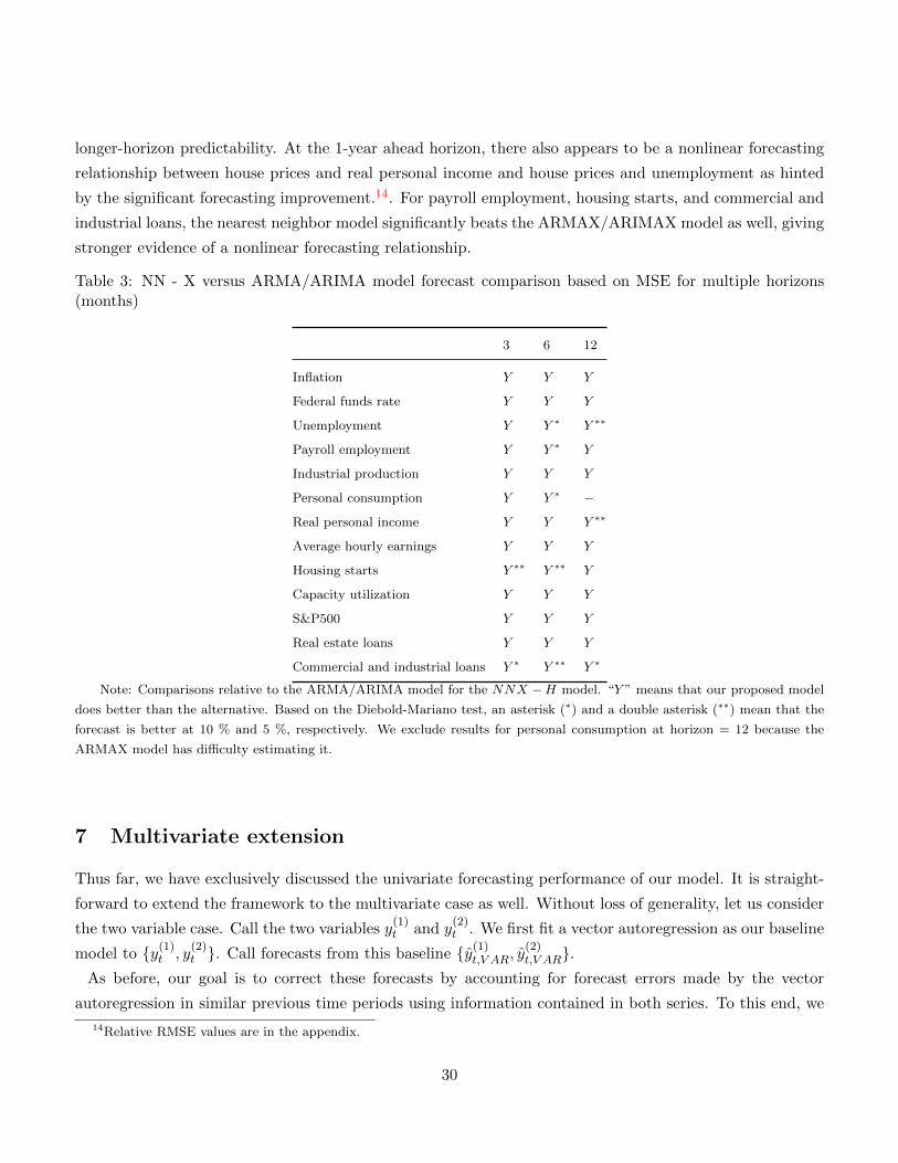
longer-horizon predictability. At the 1-year ahead horizon, there also appears to be a nonlinear forecasting

relationship between house prices and real personal income and house prices and unemployment as hinted

by the significant forecasting improvement.14. For payroll employment, housing starts, and commercial and

industrial loans, the nearest neighbor model significantly beats the ARMAX/ARIMAX model as well, giving

stronger evidence of a nonlinear forecasting relationship.

Table 3: NN - X versus ARMA/ARIMA model forecast comparison based on MSE for multiple horizons(months)

3 6 12

Inflation Y Y Y

Federal funds rate Y Y Y

Unemployment Y Y ∗ Y ∗∗

Payroll employment Y Y ∗ Y

Industrial production Y Y Y

Personal consumption Y Y ∗ −

Real personal income Y Y Y ∗∗

Average hourly earnings Y Y Y

Housing starts Y ∗∗ Y ∗∗ Y

Capacity utilization Y Y Y

S&P500 Y Y Y

Real estate loans Y Y Y

Commercial and industrial loans Y ∗ Y ∗∗ Y ∗

Note: Comparisons relative to the ARMA/ARIMA model for the NNX −H model. “Y ” means that our proposed model

does better than the alternative. Based on the Diebold-Mariano test, an asterisk (∗) and a double asterisk (∗∗) mean that the

forecast is better at 10 % and 5 %, respectively. We exclude results for personal consumption at horizon = 12 because the

ARMAX model has difficulty estimating it.

7 Multivariate extension

Thus far, we have exclusively discussed the univariate forecasting performance of our model. It is straight-

forward to extend the framework to the multivariate case as well. Without loss of generality, let us consider

the two variable case. Call the two variables y(1)t and y

(2)t . We first fit a vector autoregression as our baseline

model to {y(1)t , y(2)t }. Call forecasts from this baseline {y(1)t,V AR, y

(2)t,V AR}.

As before, our goal is to correct these forecasts by accounting for forecast errors made by the vector

autoregression in similar previous time periods using information contained in both series. To this end, we

14Relative RMSE values are in the appendix.

30

(a) Unemployment

2007.75 2008.5 2009.25 20104

5

6

7

8

9

10

(b) Inflation

2007.75 2008.5 2009.25 2010−3

−2.5

−2

−1.5

−1

−0.5

0

0.5

1

1.5

2

(c) Industrial Production

2007.75 2008.5 2009.25 2010−7

−6

−5

−4

−3

−2

−1

0

1

2

3

Greenbook nowcast (green dots), SPF nowcast (red dots), NN - X forecast with the house price index (pink diamonds), and

data (blue solid). Shaded areas are NBER recession dates. To construct the quarterly data for the unemployment rate, we take

an interquarter average of the monthly unemployment rates. To construct the same for inflation and industrial production, we

take an interquarter sum of the monthly rates.

Figure 14: Different Forecasts during the Great Recession

31

follow Mizrach (1992) and consider an extension of our original distance function to multiple variables. As

an example, consider matching the k length series ending at time t to the same length series ending at time

k 15:

dist =k∑i=1

weighs(i)

2∑j=1

((y(j)t+1−i − y

(j)t

)−(y(j)k+1−i − y

(j)k

))2The closest match now must be close for both series {y(1)t , y

(2)t } as each is weighted equally in this calcu-

lation. We standardize both series before calculating the distance measure to remove the influence of units

on the calculation.

Model selection proceeds similarly as in the univariate case. We use BIC on full sample data to select the

optimal VAR lag length with a maximum lag length of 12. We continue to use the historical out-of-sample

mean squared error to select the optimal k and m values. Since there are multiple series, we must specify

the one on which we evaluate the model’s historical forecasting performance for selection.

For our empirical exercise, we consider 2-variable VARs with each of the 13 macro and financial variables

along with the house price index. Using house price as the common variable across VARs is sensible given

the significant improvement in the univariate case upon controlling for house prices. Our data length is

the same as in the NNX-H results and the forecasting specifications remain the same. As we are primarily

interested in forecasting the 13 macro and financial variables, in each VAR, we specify that variable as the

one on which we do model selection (not the house price index).

We compare the forecasts from our model to those from a VAR in Table 4. In the multivariate case, our

methodology continues to do well. It forecasts better than the linear alternative in all but 2 cases and for 6

series, its forecasts are significantly better than those from a linear model.

Figure 15 shows the recursive one step ahead mean squared error differences between the nearest neighbor

model and the VAR for the 6 series in which the nearest neighbor model forecasts significantly better than

the VAR model. In all cases, the nearest neighbor method continues to do especially well during the Great

Recession. For inflation, industrial production, capacity utilization, and commercial and industrial loans,

the nearest neighbor model consistently outperforms the VAR model across all time periods. For housing

starts and real estate loans, however, the gains seem to be more concentrated around the Great Recession.

8 Final thoughts

Our approach performs well during sharp changes in the data and still is competitive during normal times.

We view our approach as a complement rather than a substitute to existing methods. It can be applied

in different contexts. One possible extension is to use a weighted forecast of our approach and a linear

15We focus on the match to deviations from local mean specification.

32

(a) Inflation (b) Industrial Production

1995 2000 2005 2010 2015−0.5

0

0.5

1

1.5

2

2.5

3

3.5

4

1995 2000 2005 2010 2015−0.2

0

0.2

0.4

0.6

0.8

1

1.2

(c) Housing Starts (d) Capacity Utilization

1995 2000 2005 2010 2015−100

0

100

200

300

400

500

600

1995 2000 2005 2010 2015−1

−0.5

0

0.5

1

1.5

2

2.5

3

3.5

4

(e) Real Estate Loans (f) Commercial and Industrial Loans

1995 2000 2005 2010 2015−1

0

1

2

3

4

5

1995 2000 2005 2010 2015−1

−0.5

0

0.5

1

1.5

2

2.5

3

The graphs show the relative performance of our 2-variable nearest neighbor model versus VAR in blue. Increases in these series

mean that the nearest neighbor models are doing better. The two variables are the variable listed and the house price index.

Shaded areas are NBER recession dates.

Figure 15: 2-variable nearest neighbor versus VAR model forecast comparison

33

Table 4: 2−variable nearest neighbor versus VAR model forecast comparison based on MSE (1 step ahead)

Inflation Y ∗∗

Federal funds rate N

Unemployment Y

Payroll employment Y

Industrial production Y ∗∗

Personal consumption Y

Real personal income Y

Average hourly earnings N

Housing starts Y ∗∗

Capacity utilization Y ∗∗

S&P500 Y

Real estate loans Y ∗

Commercial and industrial loans Y ∗∗

Note: Comparisons relative to the VAR model for the nearest neighbor model. The two variables are the vari-

able listed and the house price index. “Y ” means that our proposed model does better than the alternative. Based on

the Diebold-Mariano test, an asterisk (∗) and a double asterisk (∗∗) mean that the forecast is better at 10 % and 5 %, respectively.

model. The weights can be based on the probability of a recession. Clearly, this alternative gives more

emphasis to our algorithm when the economy is suffering a downturn. Alternatively, the forecasts can be

combined using the Bayesian predictive synthesis recently advocated by McAlinn and West (2016). As we

forecast better during sudden movements in the data, another possible application is to consider emerging

economies, where wild fluctuations happen more often.

34

References

Agnon, Y., A. Golan, and M. Shearer (1999): “Nonparametric, nonlinear, short-term forecasting:

theory and evidence for nonlinearities in the commodity markets,” Economics Letters, 65, 293–299.

Barkoulas, J., C. Baum, and A. Chakraborty (2003): “Nearest-Neighbor Forecasts of U.S. Interest

Rates,” Working papers, University of Massachusetts Boston.

Del Negro, M., M. Giannoni, and F. Schorfheide (2014): “Inflation in the Great Recession and New

Keynesian Models,” Staff Reports 618, Federal Reserve Bank of New York.

Del Negro, M., R. Hasegawa, and F. Schorfheide (2015): “Dynamic Prediction Pools: An Investi-

gation of Financial Frictions and Forecasting Performance,” forthcoming, Journal of Econometrics.

Del Negro, M., and F. Schorfheide (2013): “DSGE Model-Based Forecasting,” Handbook of Economic

Forecasting SET 2A-2B, p. 57.

Diebold, F., and R. Mariano (1995): “Comparing Predictive Accuracy,” Journal of Business and Eco-

nomic Statistics, 13, 253–263.

Diebold, F., and J. Nason (1990): “Nonparametric Exchange Rate Prediction?,” Journal of International

Economics, 28, 315–332.

Farmer, J. D., and J. J. Sidorowich (1987): “Predicting Chaotic Time Series,” Physical Review Letters,

59(8), 845–848.

Farmer, R. (2012): “The stock market crash of 2008 caused the Great Recession: Theory and Evidence,”

Journal of Economic Dynamics and Control, 36(5), 693 – 707.

Fernandez-Rodriguez, F., and S. Sosvilla-Rivero (1998): “Testing nonlinear forecastability in time

series: Theory and evidence from the EMS,” Economics Letters, 59(1), 49–63.

Fernandez-Rodriguez, F., S. Sosvilla-Rivero, and J. Andrada-Felix (1999): “Exchange-rate fore-

casts with simultaneous nearest-neighbour methods: evidence from the EMS,” International Journal of

Forecasting, 15(4), 383 – 392.

Ferrara, L., D. Guegan, and P. Rakotomarolayh (2010): “GDP Nowcasting with Ragged-Edge

Data: A Semi-Parametric Modeling,” Journal of Forecasting, 29, 186 – 199.

Ferrara, L., M. Marcellino, and M. Mogliani (2015): “Macroeconomic forecasting during the Great

Recession: The return of non-linearity?,” International Journal of Forecasting, 31, 664–679.

35

Frankel, J., and K. Froot (1986): “Understanding the US Dollar in the Eighties: The Expectations of

Chartists and Fundamentalists,” The Economic Record, pp. 24–38.

Gilchrist, S., and E. Zakrajsek (2012): “Credit Spreads and Business Cycle Fluctuations,” American

Economic Review, 102(4), 1692 – 1720.

Glad, I. K. (1998): “Parametrically Guided Non-Parametric Regression,” Scandinavian Journal of Statis-

tics, 25(4), 649–668.

Golan, A., and J. M. Perloff (2004): “Superior Forecasts of the U.S. Unemployment Rate Using a

Nonparametric Method,” The Review of Economics and Statistics, 86(1), 433–438.

Guerrieri, L., and M. Iacoviello (2013): “Collateral constraints and macroeconomic asymmetries,”

Discussion paper.

Hamilton, J. (1994): Time Series Analysis. Princeton University Press.

(2009): “Causes and Consequences of the Oil Shock of 2007-08,” Working paper 15002, NBER.

Hamilton, J. D. (1989): “A New Approach to the Economic Analysis of Nonstationary Time Series and

the Business Cycle,” Econometrica, 57(2), 357–84.

Lo, A., H. Mamaysky, and J. Wang (2000): “Foundations of Technical Analysis: Computational Algo-

rithms, Statistical Inference, and Empirical Implementation,” Journal of Finance, LV(4), 1705 – 1765.

Martins-Filho, C., S. Mishra, and A. Ullah (2008): “A Class of Improved Parametrically Guided

Nonparametric Regression Estimators,” Econometric Reviews, 27(4-6), 542–573.

McAlinn, K., and M. West (2016): “Dynamic Bayesian Predictive Synthesis in Time Series Forecasting,”

Working papers, Duke University.

McCracken, M. W., and S. Ng (2015): “FRED-MD: A Monthly Database for Macroeconomic Research,”

Working Papers 2015-12, Federal Reserve Bank of St. Louis.

Meade, N. (2002): “A comparison of the accuracy of short term foreign exchange forecasting methods,”

International Journal of Forecasting, 18(1), 67 – 83.

Mendoza, E. G. (2010): “Sudden Stops, Financial Crises, and Leverage,” American Economic Review,

100(5), 1941–66.

Mizrach, B. (1992): “Multivariate Nearest-Neighbour Forecast of EMS Exchange Rates,” Journal of

Applied Econometrics, 7, S151–S163.

36

Montgomery, A. L., V. Zarnowitz, R. S. Tsay, and G. C. Tiao (1998): “Forecasting the U.S.

Unemployment Rate,” Journal of the American Statistical Association, 93(442), 478–493.

Mulhern, F., and R. Caprara (1994): “A nearest neighbor model for forecasting market response,”

International Journal of Forecasting, 10, 191–207.

Murphy, K. (2012): Machine Learning: A Probabilistic Perspective. MIT Press.

Pagan, A., and A. Ullah (1999): Nonparametric Econometrics, no. 9780521355643 in Cambridge Books.

Cambridge University Press.

Potter, S. (2011): “The Failure to Forecast the Great Recession,” Liberty Street Economics Blog.

Schorfheide, F., D. Song, and A. Yaron (2014): “Identifying Long-Run Risks: A Bayesian Mixed-

Frequency Approach,” NBER Working Papers 20303, National Bureau of Economic Research, Inc.

Stock, J., and M. Watson (2007): “Why Has U.S. Inflation Become Harder to Forecast,” Journal of

Money, Credit, and Banking, 39(1), 3 – 33.

Stone, C. J. (1977): “Consistent Nonparametric Regression,” The Annals of Statistics, 5(4), 595–620.

Ullah, A., and M. Rahman (2002): “Improved Combined Parametric and Nonparametric Regressions:

Estimation and Hypothesis Testing,” Handbook of applied econometrics and statistical inference, 165, 159.

Yakowitz, S. (1987): “Nearest-neighbour methods for time series analysis,” Journal of Time Series Anal-

ysis, 8(2), 235–247.

37

A Data

All data excluding the excess bond premium and house price index runs from Jan 1959 to Jun 2015. The

final two series begin in Jan 1973.

Series Source

Civilian unemployment rate 16+ Bureau of Labor Statistics

Industrial production Federal Reserve Board

PCE Chain price index Bureau of Economic Analysis

Federal funds effective rate (Avg, annualized %) Federal Reserve Board

S&P 500 FRED-MD

Real personal consumption expenditures FRED-MD

Total nonfarm payrolls FRED-MD

Real personal income FRED-MD

Average hourly earnings FRED-MD

Housing starts FRED-MD

Capacity utilization manufacturing FRED-MD

Real estate loans FRED-MD

Commercial and industrial loans FRED-MD

Excess bond premium Simon Gilchrist website

House Price Index Robert Shiller website

Real oil price (West Texas Intermediate, deflated by PCE prices) FRED-MD

38

B Optimally selected linear baseline model

Following Ferrara, Marcellino, and Mogliani (2015), we use the BIC on the full sample data to select the

optimal baseline model within the class of ARMA/ARIMA models. We perform augmented Dickey-Fuller

tests for stationarity of the series. This test fails to reject the null of nonstationarity for the federal funds

rate, unemployment, and capacity utilization. Among those 3 series, only for the federal funds rate does the

BIC criterion select the ARIMA model over the ARMA model. We allow for up to 12 lags and 3 moving

average terms in our model selection. m is the lag length and n is the moving average term length.

Series Baseline Model ARMA(m,n)

Inflation 1, 2

Federal funds rate 8, 1, 2 (ARIMA)

Unemployment 3, 1

Payroll employment 2, 1

Industrial production 4, 2

Personal consumption 1, 2

Real personal income 0, 1

Average hourly earnings 1, 1

Housing starts 1, 2

Capacity utilization 2, 1

S&P 500 0, 1

Real estate loans 1, 2

Commercial and industrial loans 1, 2

39

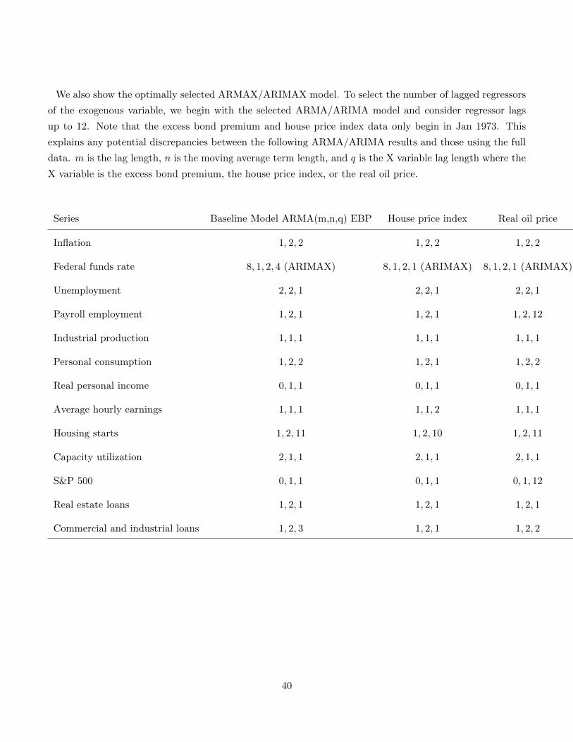
We also show the optimally selected ARMAX/ARIMAX model. To select the number of lagged regressors

of the exogenous variable, we begin with the selected ARMA/ARIMA model and consider regressor lags

up to 12. Note that the excess bond premium and house price index data only begin in Jan 1973. This

explains any potential discrepancies between the following ARMA/ARIMA results and those using the full

data. m is the lag length, n is the moving average term length, and q is the X variable lag length where the

X variable is the excess bond premium, the house price index, or the real oil price.

Series Baseline Model ARMA(m,n,q) EBP House price index Real oil price

Inflation 1, 2, 2 1, 2, 2 1, 2, 2

Federal funds rate 8, 1, 2, 4 (ARIMAX) 8, 1, 2, 1 (ARIMAX) 8, 1, 2, 1 (ARIMAX)

Unemployment 2, 2, 1 2, 2, 1 2, 2, 1

Payroll employment 1, 2, 1 1, 2, 1 1, 2, 12

Industrial production 1, 1, 1 1, 1, 1 1, 1, 1

Personal consumption 1, 2, 2 1, 2, 1 1, 2, 2

Real personal income 0, 1, 1 0, 1, 1 0, 1, 1

Average hourly earnings 1, 1, 1 1, 1, 2 1, 1, 1

Housing starts 1, 2, 11 1, 2, 10 1, 2, 11

Capacity utilization 2, 1, 1 2, 1, 1 2, 1, 1

S&P 500 0, 1, 1 0, 1, 1 0, 1, 12

Real estate loans 1, 2, 1 1, 2, 1 1, 2, 1

Commercial and industrial loans 1, 2, 3 1, 2, 1 1, 2, 2

40

In the multivariate case, we select up to lag length 12. The second variable in the VAR is the house price

index.

Series VAR(l)

Inflation 3

Federal funds rate 3

Unemployment 4

Payroll employment 3

Industrial production 3

Personal consumption 1

Real personal income 2

Average hourly earnings 3

Housing starts 1

Capacity utilization 3

S&P 500 2

Real estate loans 3

Commercial and industrial loans 3

41

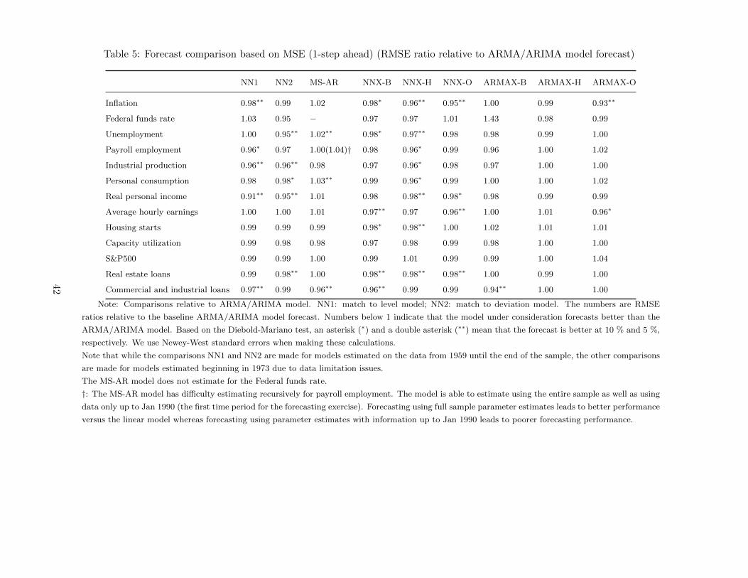
Table 5: Forecast comparison based on MSE (1-step ahead) (RMSE ratio relative to ARMA/ARIMA model forecast)

NN1 NN2 MS-AR NNX-B NNX-H NNX-O ARMAX-B ARMAX-H ARMAX-O

Inflation 0.98∗∗ 0.99 1.02 0.98∗ 0.96∗∗ 0.95∗∗ 1.00 0.99 0.93∗∗

Federal funds rate 1.03 0.95 − 0.97 0.97 1.01 1.43 0.98 0.99

Unemployment 1.00 0.95∗∗ 1.02∗∗ 0.98∗ 0.97∗∗ 0.98 0.98 0.99 1.00

Payroll employment 0.96∗ 0.97 1.00(1.04)† 0.98 0.96∗ 0.99 0.96 1.00 1.02

Industrial production 0.96∗∗ 0.96∗∗ 0.98 0.97 0.96∗ 0.98 0.97 1.00 1.00

Personal consumption 0.98 0.98∗ 1.03∗∗ 0.99 0.96∗ 0.99 1.00 1.00 1.02

Real personal income 0.91∗∗ 0.95∗∗ 1.01 0.98 0.98∗∗ 0.98∗ 0.98 0.99 0.99

Average hourly earnings 1.00 1.00 1.01 0.97∗∗ 0.97 0.96∗∗ 1.00 1.01 0.96∗

Housing starts 0.99 0.99 0.99 0.98∗ 0.98∗∗ 1.00 1.02 1.01 1.01

Capacity utilization 0.99 0.98 0.98 0.97 0.98 0.99 0.98 1.00 1.00

S&P500 0.99 0.99 1.00 0.99 1.01 0.99 0.99 1.00 1.04

Real estate loans 0.99 0.98∗∗ 1.00 0.98∗∗ 0.98∗∗ 0.98∗∗ 1.00 0.99 1.00

Commercial and industrial loans 0.97∗∗ 0.99 0.96∗∗ 0.96∗∗ 0.99 0.99 0.94∗∗ 1.00 1.00

Note: Comparisons relative to ARMA/ARIMA model. NN1: match to level model; NN2: match to deviation model. The numbers are RMSE

ratios relative to the baseline ARMA/ARIMA model forecast. Numbers below 1 indicate that the model under consideration forecasts better than the

ARMA/ARIMA model. Based on the Diebold-Mariano test, an asterisk (∗) and a double asterisk (∗∗) mean that the forecast is better at 10 % and 5 %,

respectively. We use Newey-West standard errors when making these calculations.

Note that while the comparisons NN1 and NN2 are made for models estimated on the data from 1959 until the end of the sample, the other comparisons

are made for models estimated beginning in 1973 due to data limitation issues.

The MS-AR model does not estimate for the Federal funds rate.

†: The MS-AR model has difficulty estimating recursively for payroll employment. The model is able to estimate using the entire sample as well as using

data only up to Jan 1990 (the first time period for the forecasting exercise). Forecasting using full sample parameter estimates leads to better performance

versus the linear model whereas forecasting using parameter estimates with information up to Jan 1990 leads to poorer forecasting performance.

42

Table 6: NN - X versus ARMA/ARIMA model forecast comparison based on MSE for multiple horizons(months) (RMSE ratio relative to ARMA/ARIMA model forecast)

3 6 12

Inflation 0.97 0.98 0.98

Federal funds rate 0.96 0.96 0.94

Unemployment 0.94 0.88∗ 0.80∗∗

Payroll employment 0.95 0.92∗ 0.91

Industrial production 0.96 0.98 0.98

Personal consumption 0.99 0.98∗ −

Real personal income 0.99 1.00 0.97∗∗

Average hourly earnings 0.99 1.00 0.99

Housing starts 0.99∗∗ 0.98∗∗ 0.99

Capacity utilization 0.97 0.99 0.99

S&P500 0.99 0.99 0.99

Real estate loans 0.98 0.98 0.96

Commercial and industrial loans 0.97∗ 0.96∗∗ 0.96∗

Note: Comparisons relative to the ARMA/ARIMA model for the NNX−H model. The numbers are RMSE ratios relative

to the baseline ARMA/ARIMA model forecast. Numbers below 1 indicate that the model under consideration forecasts better

than the ARMA/ARIMA model. Based on the Diebold-Mariano test, an asterisk (∗) and a double asterisk (∗∗) mean that the

forecast is better at 10 % and 5 %, respectively. We exclude results for personal consumption at horizon = 12 because the

ARMAX model has difficulty estimating.

43

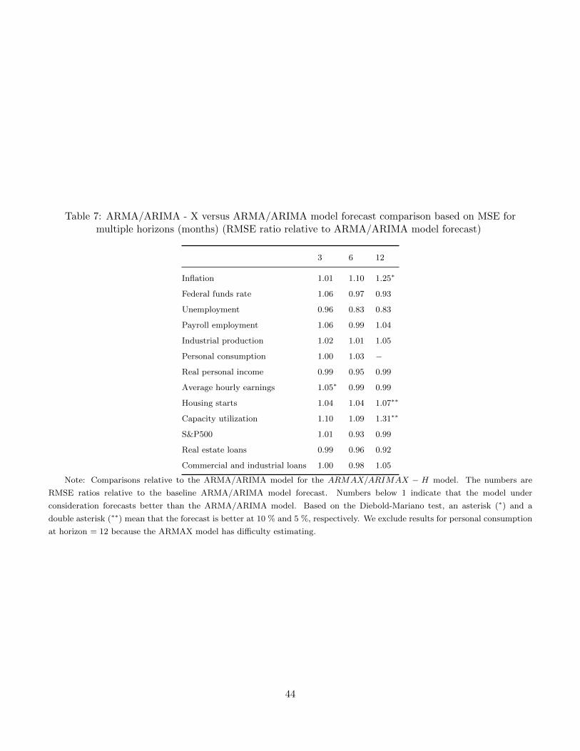
Table 7: ARMA/ARIMA - X versus ARMA/ARIMA model forecast comparison based on MSE formultiple horizons (months) (RMSE ratio relative to ARMA/ARIMA model forecast)

3 6 12

Inflation 1.01 1.10 1.25∗

Federal funds rate 1.06 0.97 0.93

Unemployment 0.96 0.83 0.83

Payroll employment 1.06 0.99 1.04

Industrial production 1.02 1.01 1.05

Personal consumption 1.00 1.03 −

Real personal income 0.99 0.95 0.99

Average hourly earnings 1.05∗ 0.99 0.99

Housing starts 1.04 1.04 1.07∗∗

Capacity utilization 1.10 1.09 1.31∗∗

S&P500 1.01 0.93 0.99

Real estate loans 0.99 0.96 0.92

Commercial and industrial loans 1.00 0.98 1.05

Note: Comparisons relative to the ARMA/ARIMA model for the ARMAX/ARIMAX − H model. The numbers are

RMSE ratios relative to the baseline ARMA/ARIMA model forecast. Numbers below 1 indicate that the model under

consideration forecasts better than the ARMA/ARIMA model. Based on the Diebold-Mariano test, an asterisk (∗) and a

double asterisk (∗∗) mean that the forecast is better at 10 % and 5 %, respectively. We exclude results for personal consumption

at horizon = 12 because the ARMAX model has difficulty estimating.

44