Embed Size (px)
Citation preview

MACRO ECONOMIC INDICATORS AND FMCG
SALES-A CASE STUDY
Submitted by:Ayan Adhikari
University of Calcutta
Department of Statistics
We are given data on FMCG Sales, which is a function of mainly 4 macro economic indicators ,
namely:
• GDP(Gross Domestic Product)
• CPI(Consumer Price Index)
• PPI(Producer Prices Index)
• IPI(Industrial Production Index) Along with them the FMCG Sales is also affected by Crude Oil Prices and Sugar Prices and the
distribution of all the above mentioned factors.
In this Case Study our objective is two fold:
1. To determine how FMCG sales gets impacted by the movement of all the above
mentioned factors
2. To predict the sales for next 3 quarters. So to achieve our objectives we carry out a statistical analysis on the data we are provided with.
A.Description of the data
The data that is provided, gives us information on FMCG Sales,which is the response
variable. The FMCG Sales however is a two dimensional vector ,consisting of the components
Value Offtake (in 00,000 Rs) and the Number of Stores .The data on FMCG Sales is given for
each month , spanning from January 2012 to June 2014. Hence,necessarily it is a Time Series
Data.
The data on the Macroeconomic Indicators,Crude Oil Prices and Sugar Prices are also
given on a monthly basis,although the data on all the covariates are not supplied for the span
January 2012 to June 2014,as in the case of the response.

The data on GDP is provided for each of the 10 quarters(There are 10 quarters from
January 2012 to June 2014).
The data on CPI(prices paid by consumers for a basket of goods and services)is given for
the span August 2013 to July 2014.Similarly the data provided on PPI(measuring the average
change in price of goods and services sold by manufacturers) and IPI(measuring changes in
output for the manufacturing,mining and utilities)are for the same time span as CPI.
So,the consolidated data may look somewhat like as below:
Month Value Offtake Number of Stores Crude Oil Sugar Pric GDP CPI PPI IPI
JAN13 1,778,946 8,756,249 5475.7 8
FEB12 1,460,671 8,373,696 5540.8 8
MAR12 1,674,358 8,370,395 5927.6 8
APR12 1,569,027 8,365,588 5892.6 6.7
MAY12 1,673,478 8,358,634 5659.7 24.3 6.7
JUN12 1,618,560 8,364,721 5083.6 24.9 6.7
JUL12 1,687,376 8,368,860 5372.2 27.9 6.1
AUG12 1,729,846 8,380,458 5849.3 25.2 6.1
SEP12 1,702,726 8,387,885 5800.7 24.3 6.1
OCT12 1,729,722 8,382,093 5475.4 23.8 5.3
NOV12 1,722,802 8,378,245 5536 23.3 5.3
DEC12 1,805,808 8,385,347 5525.5 23.2 5.3
JAN13 1,778,946 8,756,249 5705.1 22.6 5.5
FEB13 1,647,682 8,758,686 5786 21.6 5.5
MAR13 1,870,267 8,760,601 5580.7 22 5.5
APR13 1,767,852 8,766,108 5375 21.2 4.4
MAY13 1,888,606 8,765,700 5467.6 21.2 4.4
JUN13 1,810,826 8,765,753 5817.7 21.8 4.4
JUL13 1,873,960 8,765,790 6289.4 22.6 4.8
AUG13 1,907,894 8,766,110 6830.4 24.1 4.8 134.6 177.5 2.63
SEP13 1,845,721 8,770,102 6928.1 24.8 4.8 136.2 179.7 0.43
OCT13 1,909,556 8,770,151 6499.6 25.6 4.7 137.6 180.3 2.76
B.Completion of the Data Set
As it is seen from the snapshot,we mainly face 3 constraints while modeling the
impact of the movement of all the factors on FMCG Sales.They are:

A. The data contains a number of missing values in the columns of the
Covariates:Sugar Prices,IPI,CPI and PPI.
B. Moreover,the data on GDP was given on a quarterly basis.
C. However the main problem in the data was that, we were provided with the data
on FMCG Sales of January 2013 in the place of January 2012.So we have actually
treated the response data corresponding to January 2012 missing as well.
i. To overcome these problems we first consider the Response variable-FMCG Sales.
As a single value is missing among all the 30 observed data points,we replace the
values(both of Value Offtake and Number of Shops) corresponding to January 2012 by the
mean of the remaining observed data points.
Thus we obtain a dataset where we have responses corresponding to all the
observed thirty months.
Again,as the response FMCG Sales contains of two components Value Offtake and
Number of Shops,we have to actually analyse how both of them are affected by the movement
of the given Macroeconomic Factors.Or else,we can actually obtain a new response variable
Value Offtake per Shop(00,000Rs) = value offtake(00,000)/ no. of shops Here in this case study analysis,the single response variable,Value Offtake per Shop has been
considered.Thus we address one of the three constraints.
ii. Next we try to obtain the GDP values on monthly basis
For addressing this problem we first plot the GDP data given on a quarterly basis.
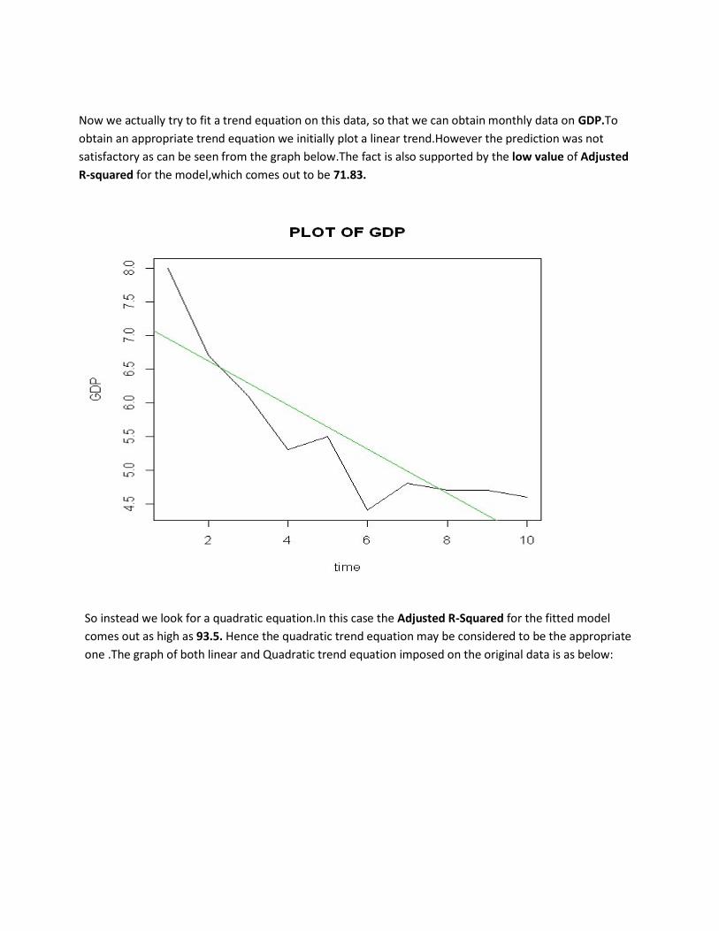
Now we actually try to fit a trend equation on this data, so that we can obtain monthly data on GDP.To
obtain an appropriate trend equation we initially plot a linear trend.However the prediction was not
satisfactory as can be seen from the graph below.The fact is also supported by the low value of Adjusted
R-squared for the model,which comes out to be 71.83.
So instead we look for a quadratic equation.In this case the Adjusted R-Squared for the fitted model
comes out as high as 93.5. Hence the quadratic trend equation may be considered to be the appropriate
one .The graph of both linear and Quadratic trend equation imposed on the original data is as below:

So we obtain a quarterly trend equation for GDP.Then we carry out the necessary
transformations and adjustments to obtain the monthly trend equation for GDP.
Quarterly Trend Equation: Yt= 8.76167-1.06598*t+0.06705*t2……….(1)
Unit:1 quarter Origin:1st quarter of 2012 Monthly Trend Equation: Yt=8.76167-((1.06598/3)*(t-(1/3)))+((0.06705/9)*((t-(1/3))2)…..(2)
Unit:1 month Origin: January 2012 In monthly trend Equation all the coefficients of time are divided by the appropriate
constants(divided by 3 as 1 quarter contains 3 months) and then properly centred.
Thus we obtain the GDP values for all the months spanning from January 2012 to June
2014from equation (2).
iii. Now,we impute the missing values in Sugar Prices,IPI,CPI,PPI
For this purpose we actually make use of the mi package(multiple imputation) in R.

Here we actually generate multiple imputations for incomplete data using iterative regression
imputation. If the variables with missingness are a matrix Y with columns Y(1), . . . , Y(K) and the
fully observed predictors are X, this entails first imputing all the missing Y values using some
crude approach (for example, choosing imputed values for each variable by randomly selecting
from the observed outcomes of that variable); and then imputing Y(1) given Y(2), . . . , Y(K) and
X; imputing Y(2) given Y(1), Y(3), . . . , Y(K) and X (using the newly imputed values for Y(1)), and
so forth, randomly imputing each variable and looping through until approximate convergence.
As we wish to impute the values of Sugar Prices,IPI,CPI and PPI,we treat them
as the Y values with missingness as mentioned in the above paragraph.To circumnavigate any
problem of Multicollinearity that may arise in future,we ignore the Oil Prices and GDP
values(both of which by now are fully observed) but take the Value Offtake per Shop only as
the fully observed predictor X,based on which the imputation is carried out.
Thus we outdo all the three initial problems that were faced at the beginning and obtain a fully
completed dataset;a snapshot of which looks as below:
Y Time Oil Sugar GDP IPI CPI PPI
0.208611 1 5475.7 25.35579 8.528097 -1.67502 140.9283 185.0866
0.174436 2 5540.8 25.25792 8.190153 1.228825 137.7208 180.3033
0.200033 3 5927.6 25.42624 7.86711 1.002539 137.9063 177.2557
0.187557 4 5892.6 25.56207 7.558967 -4.21778 139.2061 180.1868
0.20021 5 5659.7 24.3 7.265723 -0.18116 141.0971 179.4309
0.193498 6 5083.6 24.9 6.98738 -4.02633 140.6432 182.5184
0.201626 7 5372.2 27.9 6.723937 -2.08461 139.7622 180.7297
0.206414 8 5849.3 25.2 6.475393 -4.75091 138.9687 179.5387
0.202998 9 5800.7 24.3 6.24175 0.732328 132.476 182.077
0.206359 10 5475.4 23.8 6.023007 0.424546 140.9178 183.2025
0.205628 11 5536 23.3 5.819163 0.981606 137.6504 179.1849
0.215353 12 5525.5 23.2 5.63022 -4.34836 141.4364 181.2235
0.203163 13 5705.1 22.6 5.456177 -2.59397 132.5132 180.946
0.18812 14 5786 21.6 5.297033 0.257167 138.1901 179.6825
0.213486 15 5580.7 22 5.15279 1.938265 137.8538 183.4112
0.201669 16 5375 21.2 5.023447 0.219639 137.7525 182.6066
0.215454 17 5467.6 21.2 4.909003 0.529774 138.2674 181.5117
C.Analysis of the Completed dataset and fitting an
Appropriate Model Once we obtain the fully completed dataset we can actually analyse the data and study

the impact of the movement of the Macroeconomic Indicators on the FMCG Sales. We firstly plot all the Time Series data i.e, the response variables along with the six covariates.
From the above graph and the graph attached below it is evident that all the six covariates and
the response variable shows movements along time,though may not be in the same
direction.The graph of the response variable clearly shows an increasing trend with seasonality
present(presence of seasonality is natural as it is a monthly data).
Similarly the plot of OIL Prices,CPI,IPI and PPI also shows an increasing trend in the last few
quarters with certain fluctuations p resent.Also the plot of GDP clearly states that it is
decreasing over time,that is, it might affect the response negatively.The plot of Sugar Prices
also indicates of a decreasing trend with fluctuations in between.Hence Sugar Prices may also
affect the FMCG Sales negatively.

However, nothing can be said with certainty about the impact of the movement of each covariate on
FMCG Sales without carrying out a proper statistical analysis of the data. Hence to come to a concrete
conclusion we must carry out a regression analysis.
Now we check using qqplot whether the response variable can be assumed to
follow a Normal distribution or not.Here we actually compare the sample quantiles with the
theoretical quantiles.Looking at the graph below we conclude that Value Offtake per Shop

maybe well assumed to follow a Normal Distribution as all the points lie on the qqline with a
few exceptions.
Similarly we check the normality assumption for all the six Covariates.

Coefficients Estimate Standard Error p-value Decision taken
Intercept 0.6681 0.179 0.00123 Reject H0
GDP 0.1131 0.03588 0.00482 Reject H0
Value Offtake per
Shop(preeding time
point)
-0.4719 0.1387 0.00268 Reject H0
GDP(preceding time
point)
-0.1165 0.03338 0.00219 Reject H0
Sugarprices(Preceding
time point)
0.003514 0.0009913 0.00192 Reject H0
PPI -0.002009 0.0009601 0.4867 Accept H0
IPI -0.001435 .000766 0.07503 Accept H0
Oil Prices(preceding
time poiny)
-0.000007861 .000004268 0.07962 Accept H0
So it may be assumed that all the covariates as well follow approximately a Normal Distribution
as is evident from the above Q-Q Plots.
As the response follows a Normal Distribution,we may carry out a Generalized Linear
Model with the Identity Link function. However as all the data under consideration are Time
Series data we consider the Time Series regression model and use the dyn package(dynamic
regression) to carry outour necessary analysis.
"dyn" enables regression functions that were not written to handle time series to
handle them. Both the dependent and independent variables may be time series and they may
have different time indexes (in which case they are automatically aligned).
We go on adding one variable at a time to obtain the most parsimonious model,that might
explain the impact of the movement of the covariates on the response.
But we do face a problem in our pursuit to seek for the best predictive equation.The
best model that we obtain in terms of minimum AIC and residual deviance does not include all
the factors,but is a function of GDP,Response of the preceding time point,GDP of the
preceding time point , Sugar Prices of the preceding time point,PPI,IPI and Oil Prices of the
preceding time point.
The best model obtained by incorporating all the covariates do also admit a low AIC but it
is greater than the above mentioned model.
A statistical table of the following two models is presented here:
I. The best model:Model I

Here the null hypothesis states that H0:the particular coefficient is 0.So we conclude from the
above table that all the covariates except PPI,IPI and Oil Prices at the preceding time point are
significant,at 5% level of significance.The measures of Goodness of fit is provided by AIC and
residual deviance.They comes out to be as
AIC:-203.22 Residual Deviance: 0.00082608 on 21 df Hence the model comes out to be :
Yt=0.6681+0.1131*GDPt-0.4719*Yt-1-0.1165*GDPt-1+0.003514*Sugart-1-0.002009*PPIt-
0.001435*IPIt-0.000007861*Oilt-1
II. The best model including all the covariates:Model II
Coefficients Estimate Standard Error p-Value Decision
Intercept 0.6267 0.2048 0.00617 Reject H0
GDP .1075 .03868 0.01158 Reject H0
Value Offtake per
Shop(preceding
time point)
-0.4833 .1437 0.00309 Reject H0
GDP(preceding
time point)
-.1112 .03606 0.00587 Reject H0
CPI 0.0004369 0.0009795 0.66037 AcceptH0
PPI -.002113 .001006 0.04859 Reject H0
Sugar
Prices(Preceding
time point)
.003419 0.001033 0.00349 Reject H0
Oil Prices(Preceding
time point)
-.000006989 .00000477 0.15843 Accept H0
IPI -0.001431 .0007811 0.08193 AcceptH0
Here the null hypothesis states that H0:the particular coefficient is 0.So we conclude from the
above table that all the covariates except CPI,Oil Prices at the preceding time point and IPI are
significant,at 5% level of significance.The measures of Goodness of fit is provided by AIC and
residual deviance.They comes out to be as
AIC:-201.51 Residual Deviance: 0.0008179on 20 df Hence the model comes out to be :
Yt=0.6267+.1075*GDPt-0.4833*Yt-1-.1112*GDPt-1+0.0004369*CPIt- .002113*PPIt
+.003419*Sugar t-1-.000006989*Oil t-1-0.001431*IPIt

D.The Conclusion
The graph of the actual and the fitted values are shown below:
So from the graph we can conclude that the fitted model do serve as a good prediction formula
at the beginning and end of the time span,though may fail to do so accurately in the
middle.However both the fitted models can actually predict the rises and declines in the FMCG
Sales over time.As there is not much deviation between the best model and the best model
obtained by using all the Covariate values,we will consider model II as the desired model as it
accurately gives the impact of movement of all the covariates on the FMCG Sales.

The model which is given as :
Yt=0.6267+.1075*GDPt-0.4833*Yt-1-.1112*GDPt-1+0.0004369*CPIt- .002113*PPIt
+.003419*Sugar t-1-.000006989*Oil t-1-0.001431*IPIt
may be interpreted as below.
We see from the above model that the Value Offtake per shop is positively correlated
with GDP,CPI and Sugar Price(of the preceding year).The interpretation may be as follows:
The FMCG Sales increases as the GDP for that particular time point increases, i.e., as
there is growth in the economy,the Sales increases.Also as CPI increases,or in other words the
amount of money paid by a consumer for a basket of goods and services increases,so does
FMCG Sales ,as is very evident from the increased spending power of the consumers.The Sugar
price of the preceding time point also do positively affect the FMCG Sales.
On the other hand the response is negatively affected by the Value Offtake per shop of
the preceding time point,GDP of the preceding time point,PPI,Oil Price of the preceding time
point and IPI.
That both the Value Offtake per shop of the preceding time point and GDP of the
preceding time point affect the response negatively,well establishes the fact that the response
at a particular time point is indeed positively affected by the GDP at that time point.However
if the Sales is one month is low it may result in increased Sale during the successive month.On
the other hand as PPI increases, i,e., the producer’s price increases the demand decreases and
hence it results in decreased Sales.
The value of the fitted and actual response variables are also provided herewith:
ACTUAL DATA FITTED DATA
0.174436 0.1761853
0.200033 0.1977128
0.187557 0.1846241
0.20021 0.2062007
0.193498 0.1911048
0.201626 0.2035335
0.206414 0.2062317
0.202998 0.1995788
0.206359 0.2055571
0.205628 0.2065550
0.215353 0.2064828
0.203163 0.2030951

0.18812 0.2058080
0.213486 0.2115194
0.201669 0.2028833
0.215454 0.2129214
0.20658 0.2055969
0.213781 0.2162724
0.217644 0.2117013
0.210456 0.2122387
0.217734 0.2152377
0.218895 0.2230590
0.230446 0.2253755
0.221738 0.2125913
0.202495 0.2121646
0.232641 0.2306643
0.212545 0.2199740
0.22655 0.2248898
0.217588 0.2153383
Thus we have achieved our 1st objective of assessing the impact of the movement of the
Macroeconomic Indicators on the FMCG Sales .
Now we move onto our second objective:Predict the sales for the next 3 quarters.
To achieve this objective,we actually make use of the model that we have proposed in
the earlier section.
Yt=0.6267+.1075*GDPt-0.4833*Yt-1-.1112*GDPt-1+0.0004369*CPIt- .002113*PPIt
+.003419*Sugar t-1-.000006989*Oil t-1-0.001431*IPIt
But here the covariate values are unknown as well.But as all the variables are necessarily Time
Series data,we may make use of the different Time Series tools to actually predict their future
values,and then replace them in the model to obtain the predicted sales for the upcoming 3
quarters.
In R we use the tseries package to carry out the DICKEY FULLER TEST to find out the
appropriate value of the differencing operator d or the number of times the given data set has
to be differenced to obtain a stationary Time Series.Then we use the forecast package to find

out the appropriate ARIMA model that needs to be fitted to the data.Once we obtain the
appropriate model,the value of the upcoming 9 months can be predicted.
However incase of CPI,PPI and IPI we were already provided with the data of July 2014,so we
need to predict only the upcoming 8 values.
As in case of GDP although we make use of the monthly trend equation to obtain the future
values.
The appropriate models:
• Oil Prices: Here we find the appropriate value of d=2 and an ARIMA(0,2,0) model is most suitable for the
given data.
The AIC of the fitted model is 404.44.The completed dataset is: Jan Feb Mar Apr May Jun Jul Aug Sep Oct N ov
5475.7 5540.8 5927.6 5892.6 5659.7 5083.6 5372.2 5849.3 5800.7 5475.4 5536.0
5705.1 5786.0 5580.7 5375.0 5467.6 5817.7 6289.4 6830.4 6928.1 6499.6 6432.7
6683.9 6777.2 6548.5 6333.8 6274.3 6471.1 6667.9 6864.7 7061.5 7258.3 7455.1
7848.7 8045.5 8242.3
Dec
5525.5
6534.9
7651.9
• Sugar Prices
Here we find the appropriate value of d=2 and an ARIMA(2,2,0) model is most suitable for the
given data.
The model is given as
Xt+0.5624*Xt-1+0.5533*Xt-2=εt
The AIC of the fitted model is 104.42.The completed dataset is:

Jan Feb Mar Apr May Jun Jul Aug
25.04605
23.58084
24.21894
26.11498
24.30000
24.90000
27.90000
25.20000
22.60000 21.60000 22.00000 21.20000 21.20000 21.80000 22.60000 24.10000
21.40000
23.20000
24.10000
24.30000
23.90000
23.90000
24.00702
23.83255
23.59418
23.53607
23.46656
Sep
Oct
Nov
Dec
24.30000 23.80000 23.30000 23.20000
24.80000
25.60000
24.50000
22.50000
23.75716
•
23.78180
IPI
23.69536
23.61605
Here we find the appropriate value of d=2 and an ARIMA(0,2,2) model is most suitable for the
given data.
The model is given as
Xt=εt +1.5547*ε t-1- 0.6115* εt-2
The AIC of the fitted model is 142.94.The completed dataset is:
Jan Feb Mar Apr May Jun Jul
1.1746550 7.3972661 3.7072634 2.8963077 4.4504296 4.0884881 3.9991053
2.4120624 0.5958998 0.6001720 0.2831000 -1.0973953 3.5172673 -0.6028610
-0.1600000 0.8000000 -1.8000000 -0.5000000 3.4000000 4.7000000 3.4000000
5.0022741 5.3438301 5.6853862 6.0269422
Aug Sep Oct Nov Dec
5.8232911 2.3769340 3.9591879 3.4029745 -0.9656482
2.6300000 0.4300000 2.7600000 -1.1600000 -1.3200000
3.4000000 3.6360501 3.9776061 4.3191621 4.6607181

• CPI
Here we find the appropriate value of d=2 and an ARIMA(3,2,1) model is most suitable for the
given data.
The model is given as
Xt+0.2641*Xt-1+0.4580*Xt-2+0.52*Xt-3=εt +0.7508*ε t-1
The AIC of the fitted model is 120.2.The completed dataset is:
Jan Feb Mar Apr May Jun Jul Aug
138.2053 138.7676 136.1041 136.7705 138.4375 136.9388 136.7875 137.8282
139.5952 137.3964 136.6392 136.3946 140.7071 140.5282 138.1013 134.6000
137.4000 137.3000 138.1000 139.1000 139.9000 141.2000 143.7000 143.7000
147.1355 147.3322 148.1754 149.3200
Sep Oct Nov Dec
140.5583 137.9624 137.3509 138.4425
136.2000 137.6000 139.4000 138.0000
143.5506 143.9616 145.5932 146.7234
• PPI
Here we find the appropriate value of d=1 and a SARIMA model is most suitable for the
given data.
The AIC of the fitted model is 119.16.The completed dataset is:
Jan Feb Mar Apr May Jun Jul Au g 177.8320 179.4753 177.8159 179.9181 176.3337 179.6239 179.4277 180.3901
179.0016 180.7789 180.5083 181.2937 181.4430 179.2461 179.2569 177.5000
178.9000 178.9000 179.8000 180.2000 181.7000 182.6000 184.6000 184.6000
185.0593 185.2501 185.4410 185.6318

Sep Oct Nov Dec
180.5875
176.8029
177.2197
180.7103
179.7000
180.3000 181.5000 179.2000
184.2959
184.4867
184.6776
184.8684
•
GDP
The GDP is calculated from the monthly trend equation and the completed dataset is as
follows:
8.528097 8.190153 7.867110 7.558967 7.265723 6.987380 6.723937 6.475393
6.241750 6.023007 5.819163 5.630220 5.456177 5.297033 5.152790 5.023447
4.909003
4.809460
4.724817
4.655073
4.600230
4.560287
4.535243
4.525100
4.529857
4.549513
4.584070
4.633527
4.697883
4.777140
4.871297
4.980353
5.104310
5.243167
5.396923
5.565580
5.749137
5.947593
6.160950
As soon as all the Covariates are obtained,we obtain the Predictes sales value of the
upcoming3 quarters using the model
Yt=0.6267+.1075*GDPt-0.4833*Yt-1-.1112*GDPt-1+0.0004369*CPIt-
.002113*PPIt+.003419*Sugar t-1-.000006989*Oil t-1-0.001431*IPIt
They are as follows:
Month Value Offtake per Stores(Predicted)
July 2014 0.218195
Aug 2014 0.2399177
Sep 2014 0.2223075
Oct 2014 0.2269519
Nov 2014 0.2184703
Dec 2014 0.2263709
Jan 2015 0.2227174
Feb 2015 0.2202478
Mar 2015 0.2196627

The graph of the total Sales is as given below:
Thus we have achieved our 2nd objective as well.